Analytical Background

John C.S. Lui

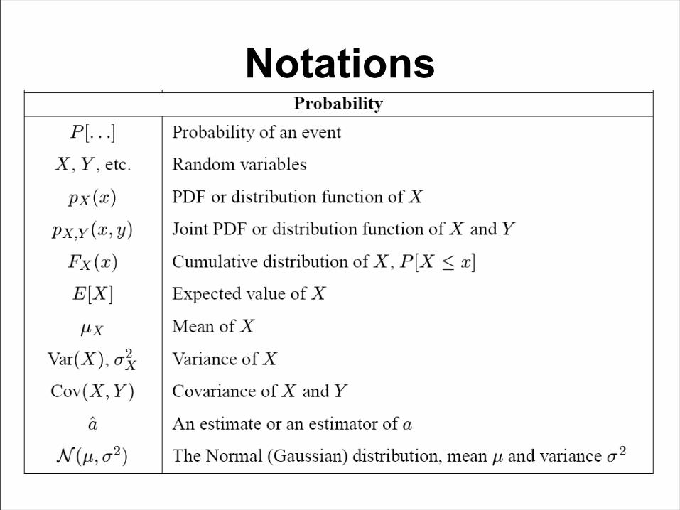
Notations

Random variable & CDF

• Definition: is the outcome of a random event or experiment that yields a numeric values.

• For a given x, there is a fixed possibility that the random variable will not exceed this value, written as P[X<=x].

• The probability is a function of x, known as FX(x). FX(.) is the cumulative distribution function (CDF) of X.

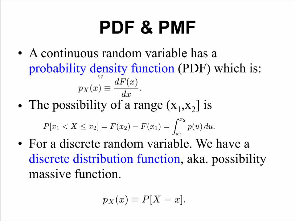
PDF & PMF• A continuous random variable has a

probability density function (PDF) which is:

• The possibility of a range (x1,x2] is

• For a discrete random variable. We have a discrete distribution function, aka. possibility massive function.

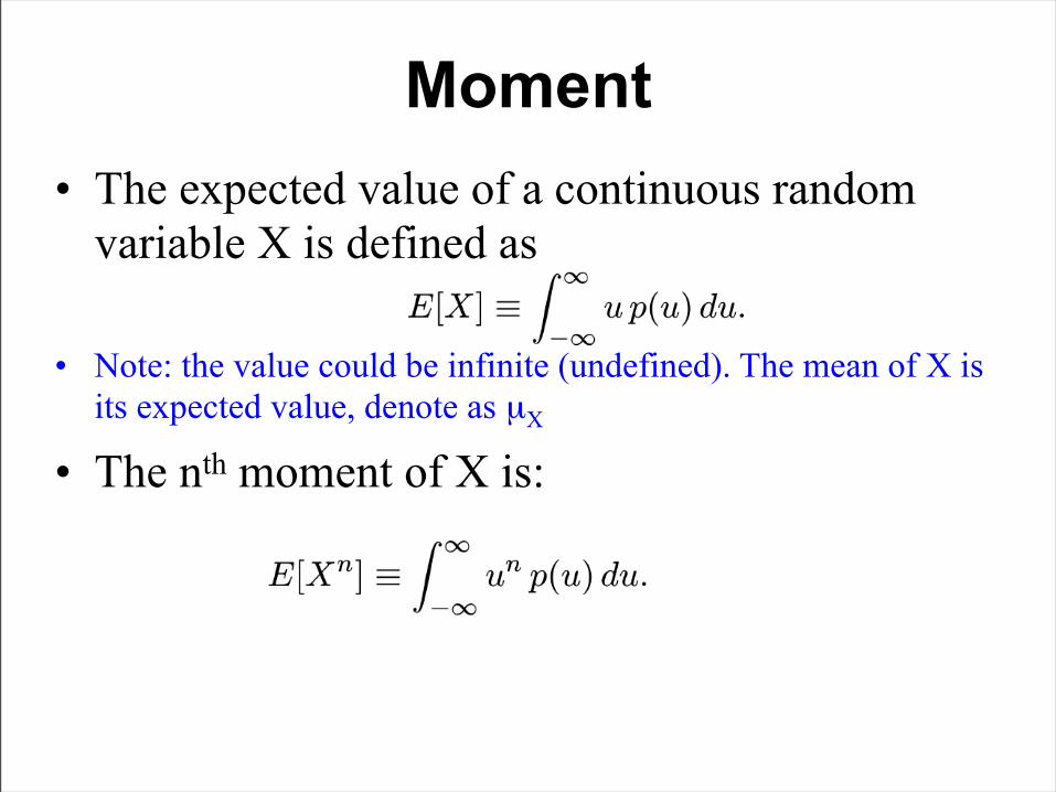
Moment• The expected value of a continuous random

variable X is defined as

• Note: the value could be infinite (undefined). The mean of X is its expected value, denote as µX

• The nth moment of X is:

Variability of a random variable

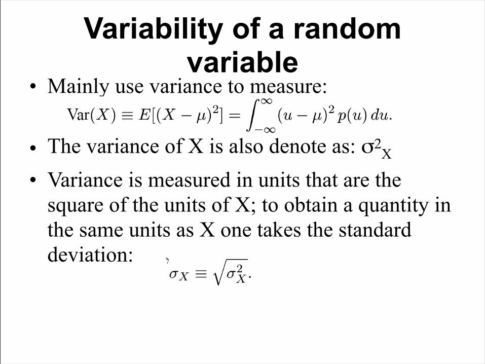
• Mainly use variance to measure:

• The variance of X is also denote as: σ2X

• Variance is measured in units that are the square of the units of X; to obtain a quantity in the same units as X one takes the standard deviation:

Joint probability

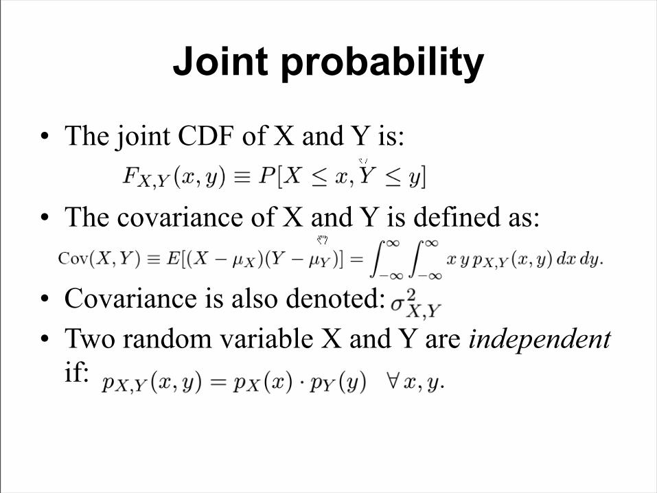
• The joint CDF of X and Y is:

• The covariance of X and Y is defined as:

• Covariance is also denoted:• Two random variable X and Y are independent

if:

Conditional Probability

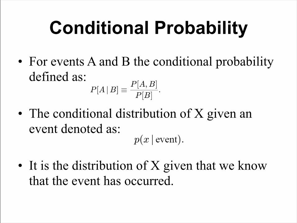
• For events A and B the conditional probability defined as:

• The conditional distribution of X given an event denoted as:

• It is the distribution of X given that we know that the event has occurred.

Conditional Probability (cont.)

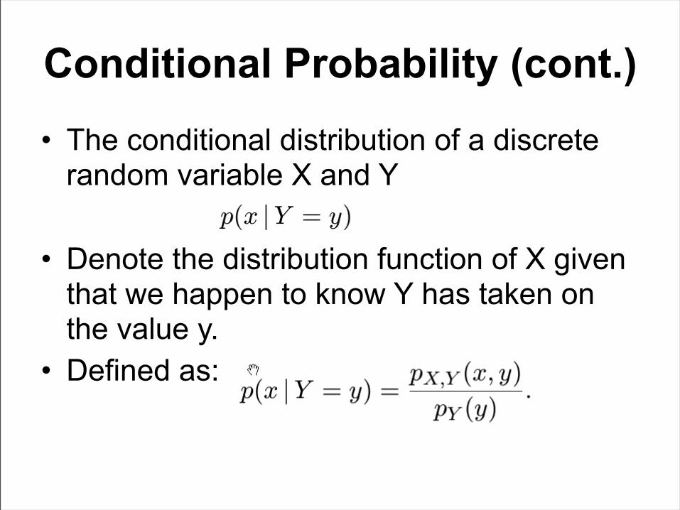
• The conditional distribution of a discrete random variable X and Y

• Denote the distribution function of X given that we happen to know Y has taken on the value y.

• Defined as:

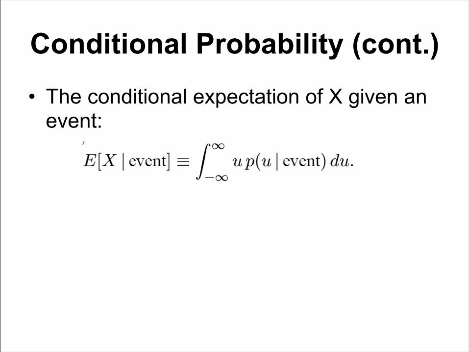
Conditional Probability (cont.)

• The conditional expectation of X given an event:

Central Limit Theorem

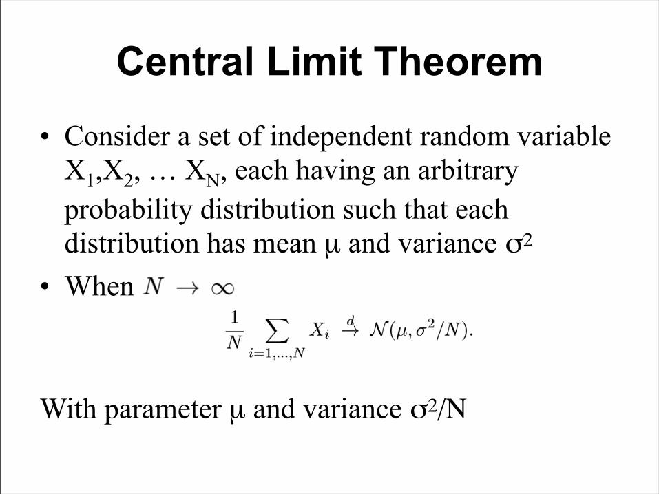
• Consider a set of independent random variable X1,X2, … XN, each having an arbitrary probability distribution such that each distribution has mean µ and variance σ2

• When

With parameter µ and variance σ2/Ν

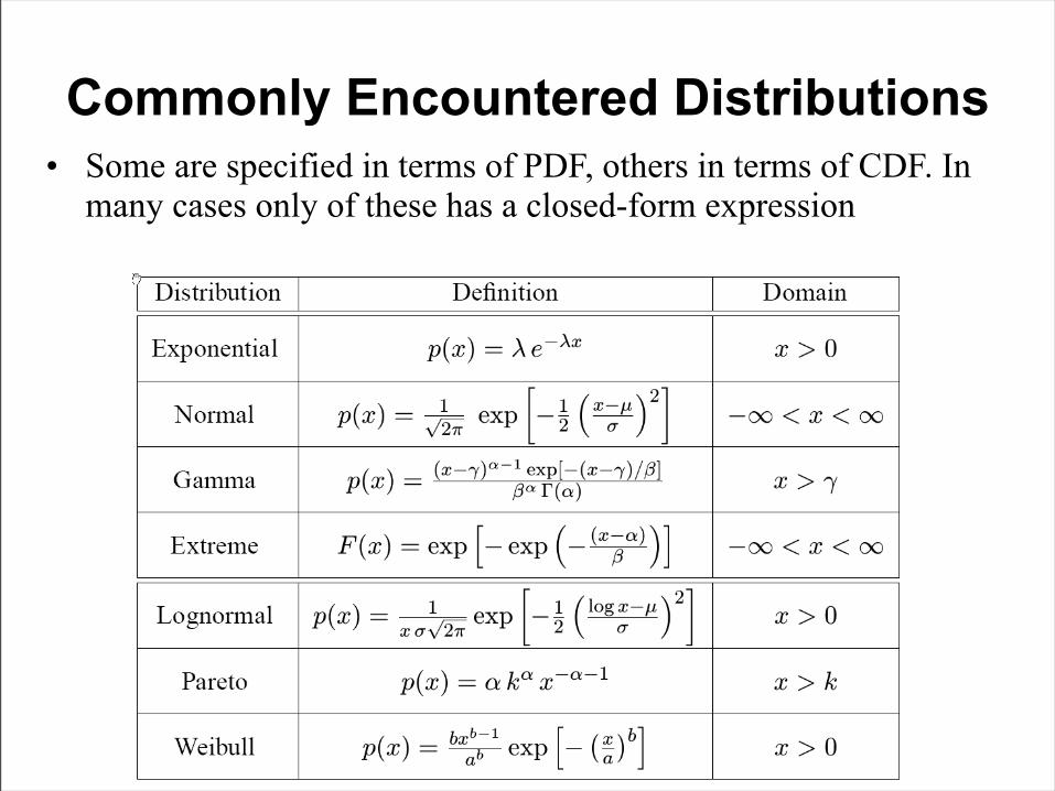
Commonly Encountered Distributions• Some are specified in terms of PDF, others in terms of CDF. In

many cases only of these has a closed-form expression

Stochastic Processes

• Stochastic process: a sequence of random variables, such a sequence is called a stochastic process.

• In Internet measurement, we may encounter a situation in which measurements are presented in some order; typically such measurements arrived.

Stochastic Processes

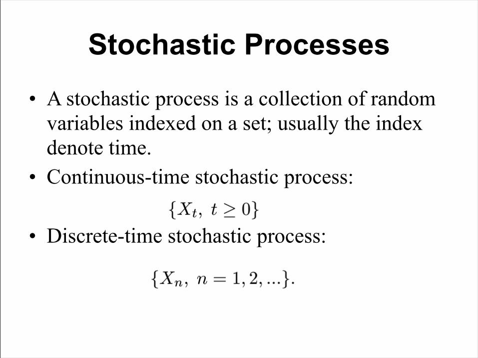
• A stochastic process is a collection of random variables indexed on a set; usually the index denote time.

• Continuous-time stochastic process:

• Discrete-time stochastic process:

Stochastic Processes

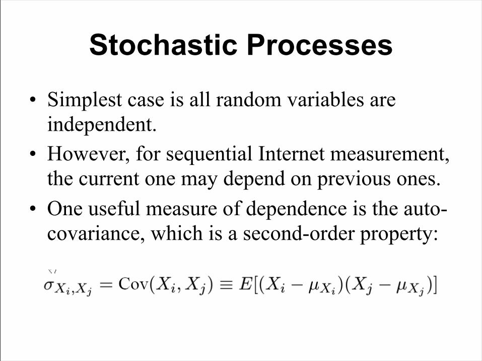
• Simplest case is all random variables are independent.

• However, for sequential Internet measurement, the current one may depend on previous ones.

• One useful measure of dependence is the auto-covariance, which is a second-order property:

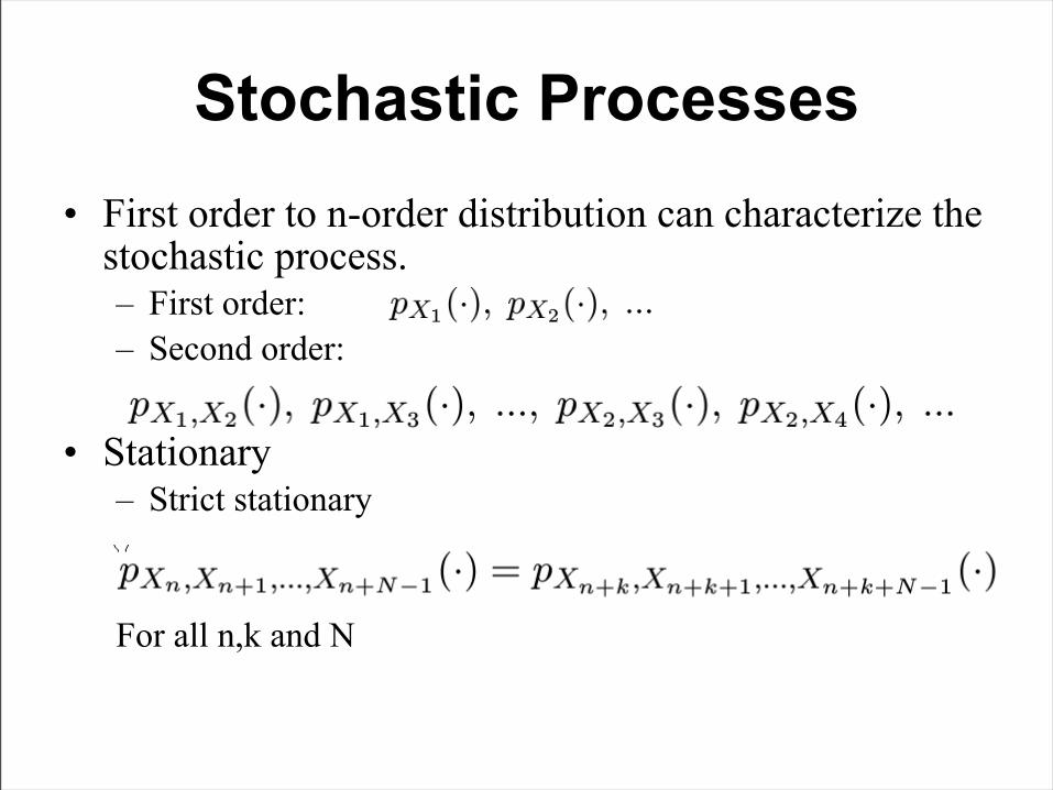
Stochastic Processes• First order to n-order distribution can characterize the

stochastic process.– First order:– Second order:

• Stationary– Strict stationary

For all n,k and N

Stochastic Processes

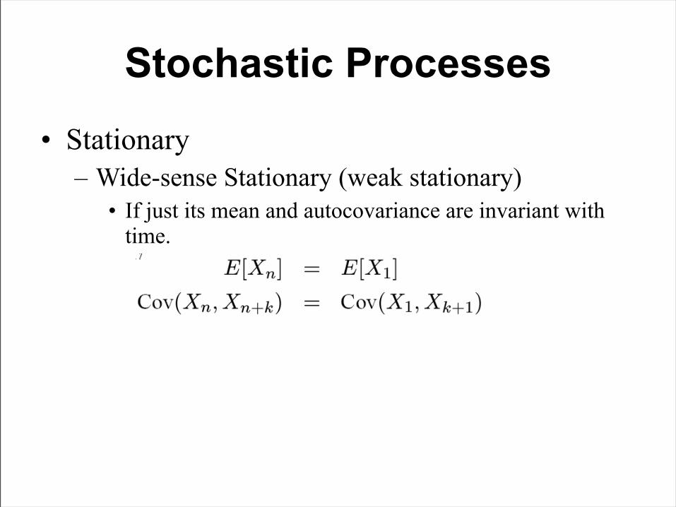
• Stationary– Wide-sense Stationary (weak stationary)

• If just its mean and autocovariance are invariant with time.

Stochastic Processes

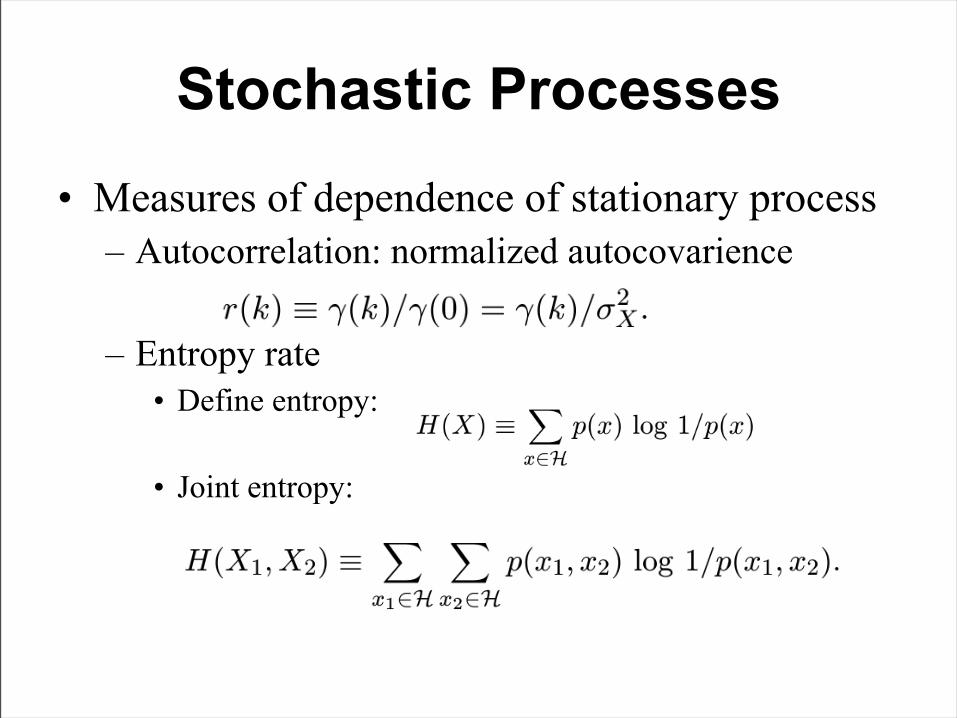
• Measures of dependence of stationary process– Autocorrelation: normalized autocovarience

– Entropy rate• Define entropy:

• Joint entropy:

Stochastic Processes

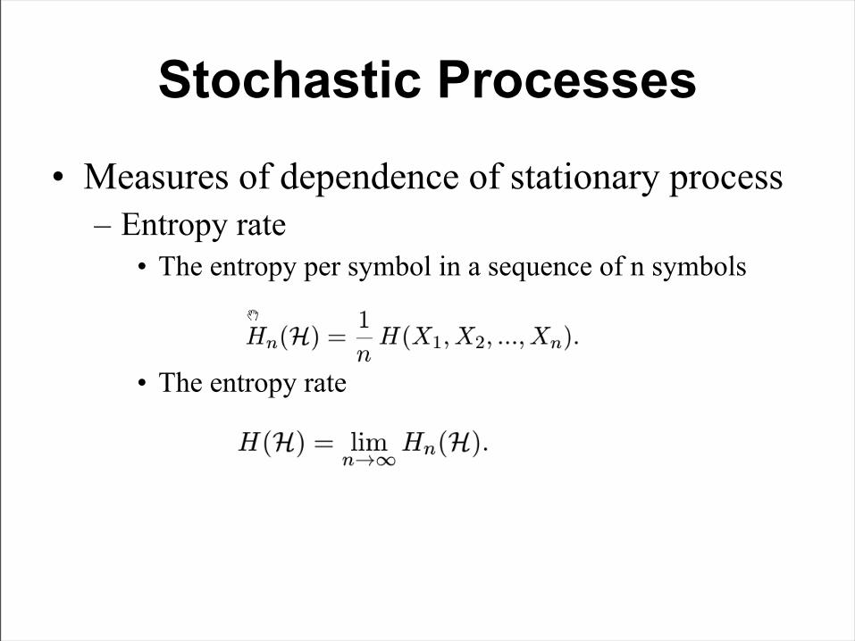
• Measures of dependence of stationary process– Entropy rate

• The entropy per symbol in a sequence of n symbols

• The entropy rate

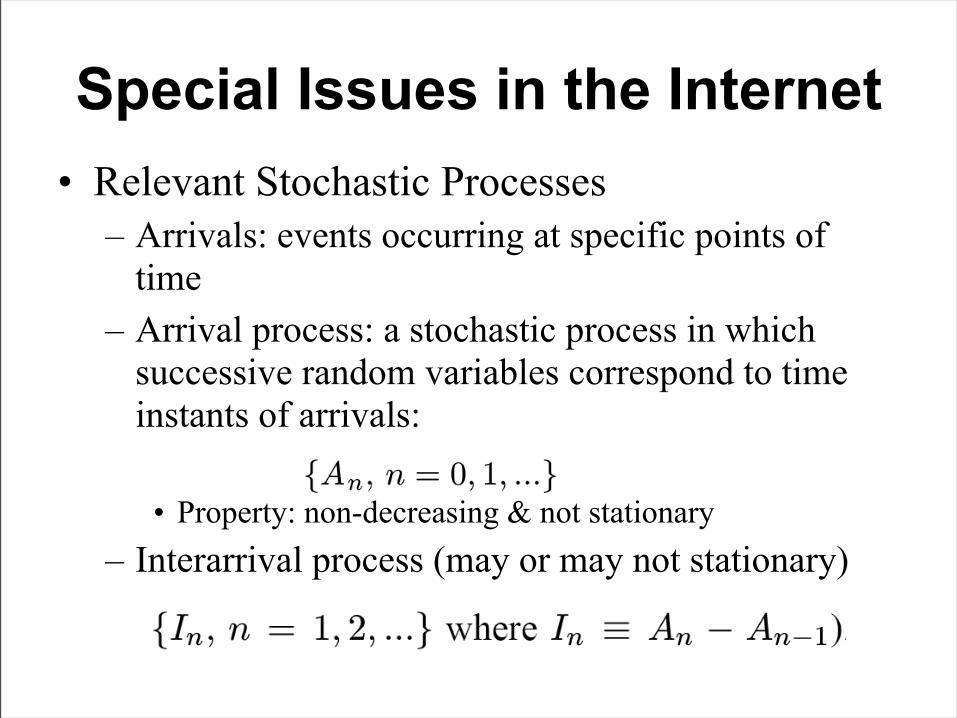
Special Issues in the Internet• Relevant Stochastic Processes

– Arrivals: events occurring at specific points of time

– Arrival process: a stochastic process in which successive random variables correspond to time instants of arrivals:

• Property: non-decreasing & not stationary– Interarrival process (may or may not stationary)

Special Issues in the Internet

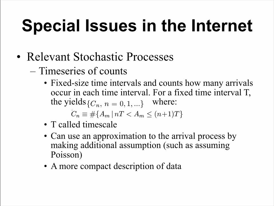
• Relevant Stochastic Processes– Timeseries of counts

• Fixed-size time intervals and counts how many arrivals occur in each time interval. For a fixed time interval T, the yields where:

• T called timescale• Can use an approximation to the arrival process by

making additional assumption (such as assuming Poisson)

• A more compact description of data

Short tails and Long tails

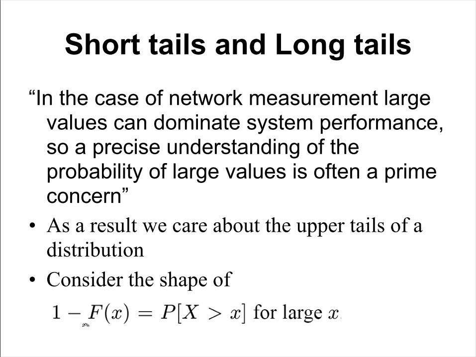
“In the case of network measurement large values can dominate system performance, so a precise understanding of the probability of large values is often a prime concern”

• As a result we care about the upper tails of a distribution

• Consider the shape of

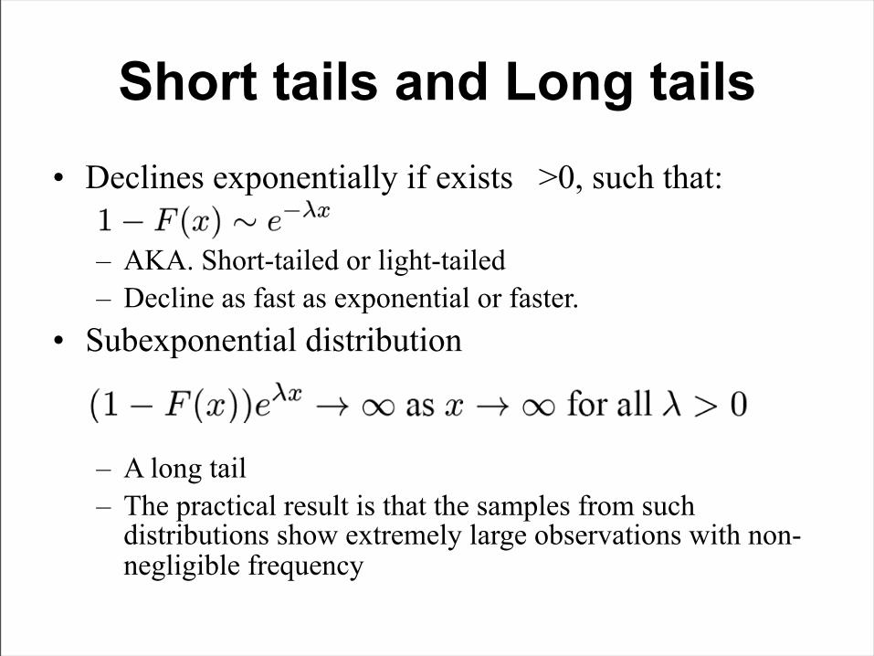
Short tails and Long tails• Declines exponentially if exists >0, such that:

– AKA. Short-tailed or light-tailed– Decline as fast as exponential or faster.

• Subexponential distribution

– A long tail– The practical result is that the samples from such

distributions show extremely large observations with non-negligible frequency

Short tails and Long tails

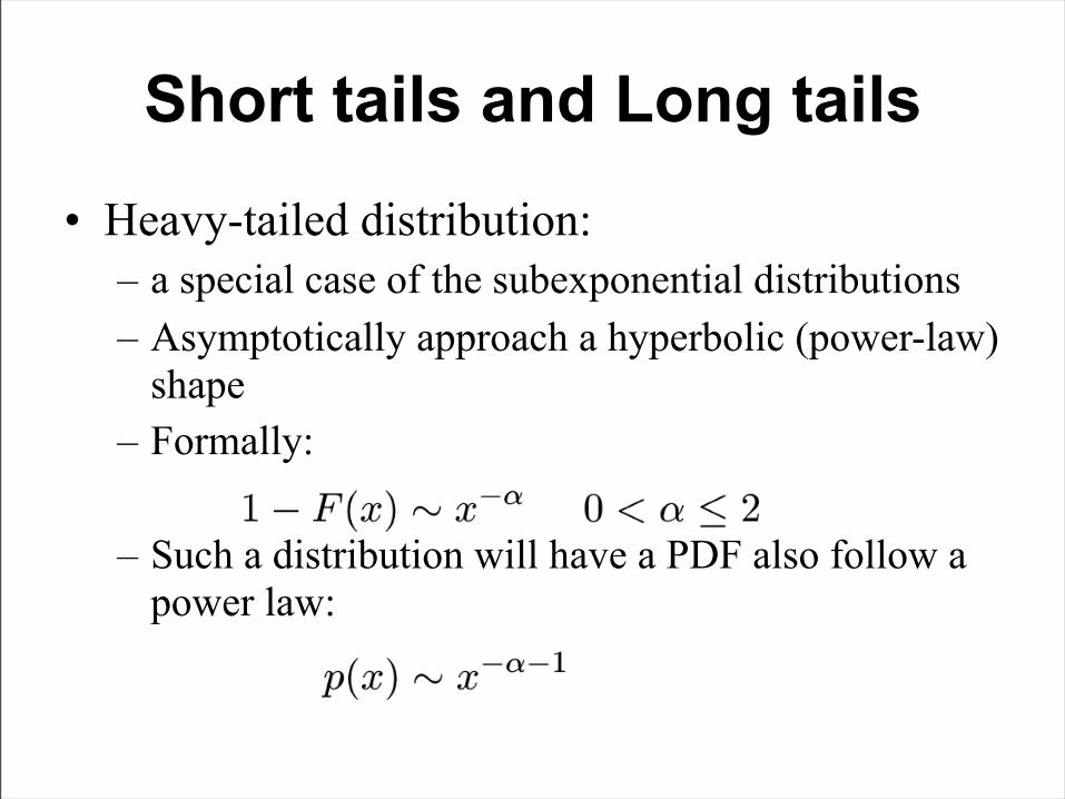
• Heavy-tailed distribution: – a special case of the subexponential distributions– Asymptotically approach a hyperbolic (power-law)

shape– Formally:

– Such a distribution will have a PDF also follow a power law:

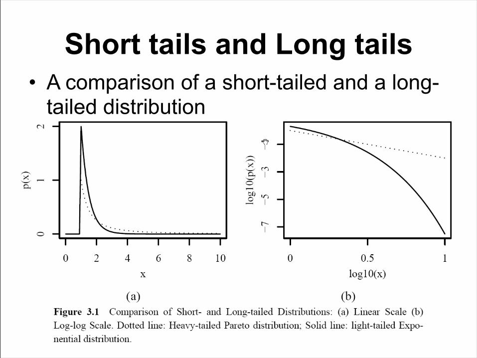
Short tails and Long tails• A comparison of a short-tailed and a long-

tailed distribution

Statistics

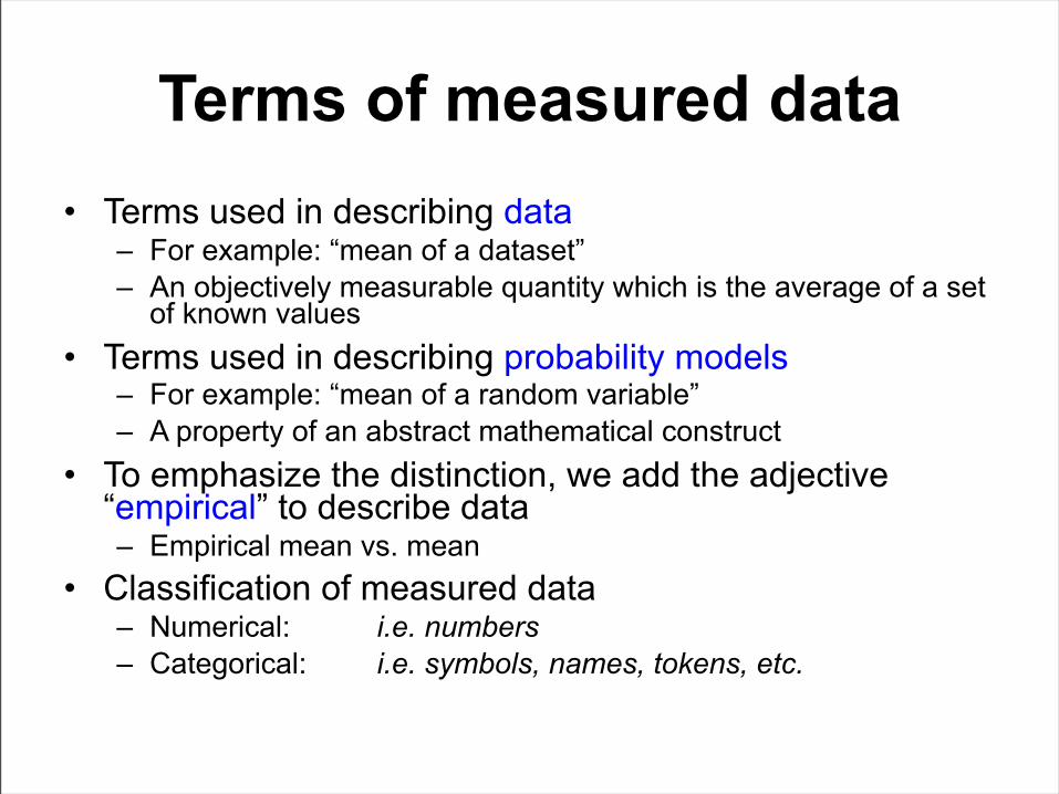
Terms of measured data• Terms used in describing data

– For example: “mean of a dataset”– An objectively measurable quantity which is the average of a set

of known values• Terms used in describing probability models

– For example: “mean of a random variable”– A property of an abstract mathematical construct

• To emphasize the distinction, we add the adjective “empirical” to describe data– Empirical mean vs. mean

• Classification of measured data– Numerical: i.e. numbers– Categorical: i.e. symbols, names, tokens, etc.

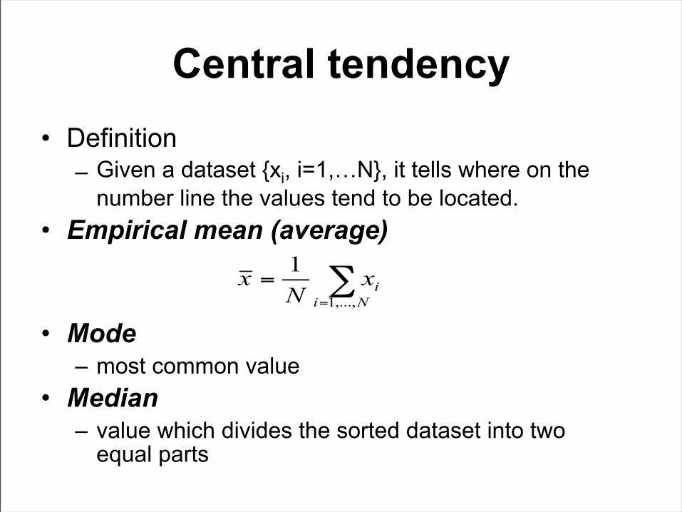
Central tendency• Definition

– Given a dataset {xi, i=1,…N}, it tells where on the number line the values tend to be located.

• Empirical mean (average)

• Mode– most common value

• Median– value which divides the sorted dataset into two

equal parts

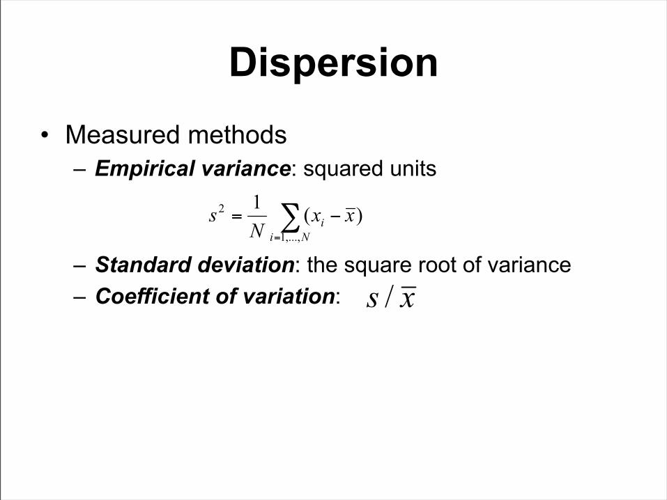
Dispersion• Measured methods

– Empirical variance: squared units

– Standard deviation: the square root of variance– Coefficient of variation:

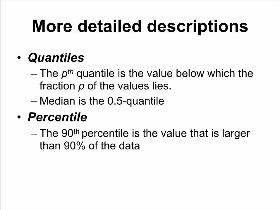
More detailed descriptions

• Quantiles– The pth quantile is the value below which the

fraction p of the values lies.– Median is the 0.5-quantile

• Percentile– The 90th percentile is the value that is larger

than 90% of the data

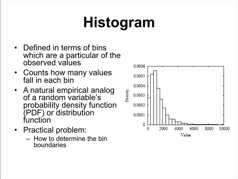
Histogram• Defined in terms of bins

which are a particular of the observed values

• Counts how many values fall in each bin

• A natural empirical analog of a random variable’s probability density function (PDF) or distribution function

• Practical problem: – How to determine the bin

boundaries

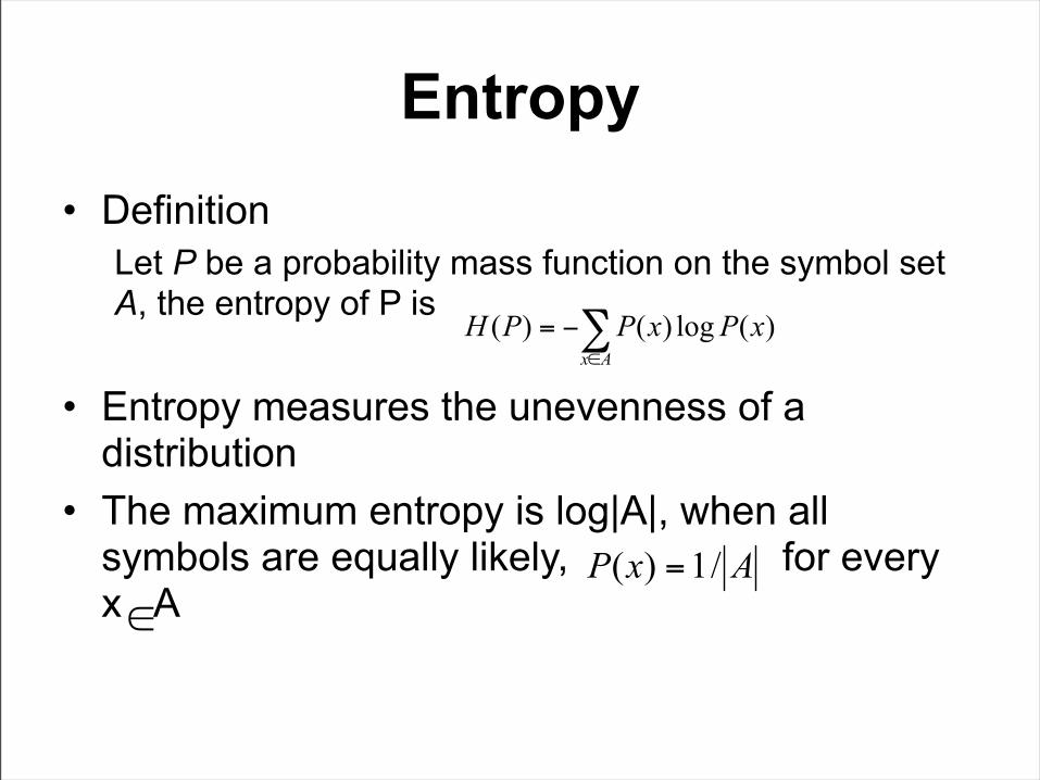
Entropy• Definition

Let P be a probability mass function on the symbol set A, the entropy of P is

• Entropy measures the unevenness of a distribution

• The maximum entropy is log|A|, when all symbols are equally likely, for every x A

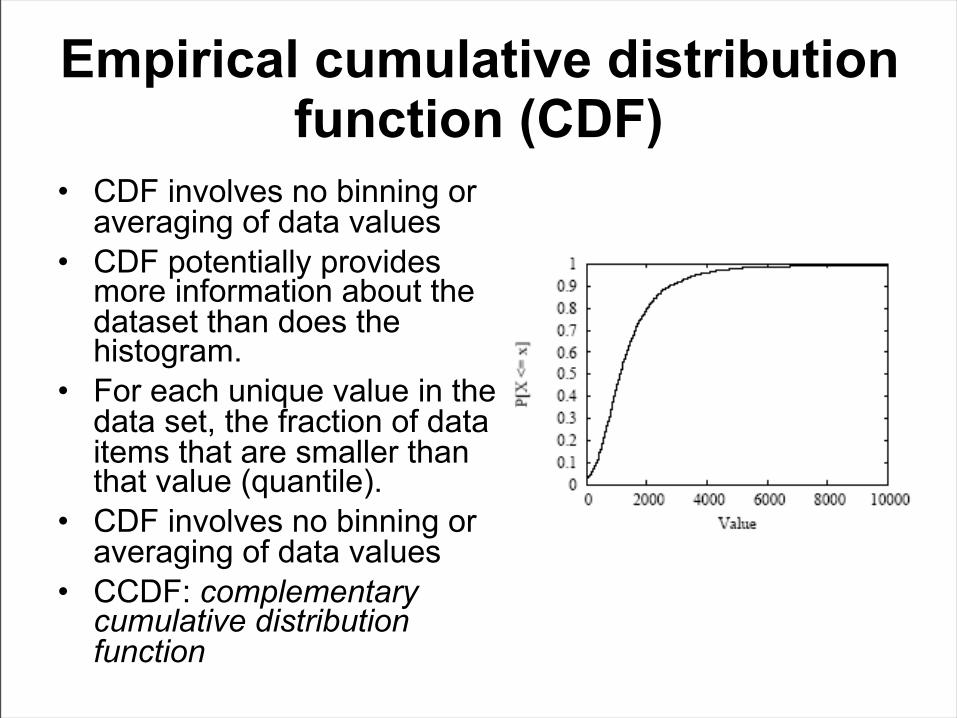
Empirical cumulative distribution function (CDF)

• CDF involves no binning or averaging of data values

• CDF potentially provides more information about the dataset than does the histogram.

• For each unique value in the data set, the fraction of data items that are smaller than that value (quantile).

• CDF involves no binning or averaging of data values

• CCDF: complementary cumulative distribution function

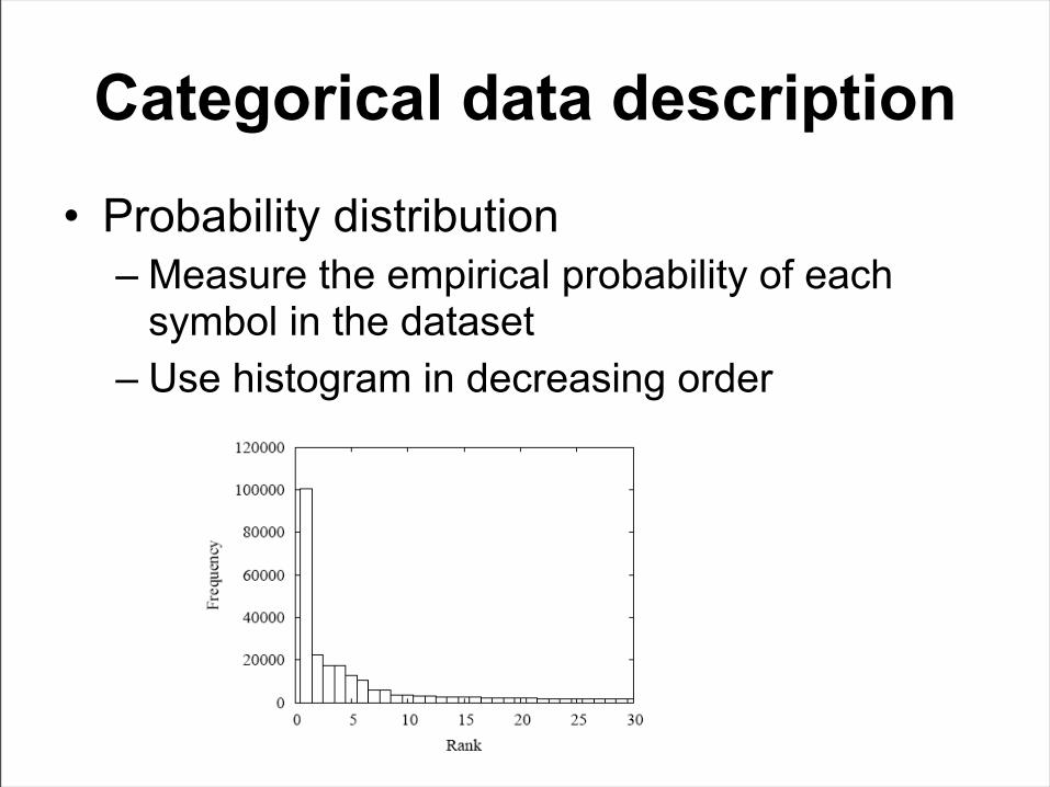
Categorical data description

• Probability distribution– Measure the empirical probability of each

symbol in the dataset– Use histogram in decreasing order

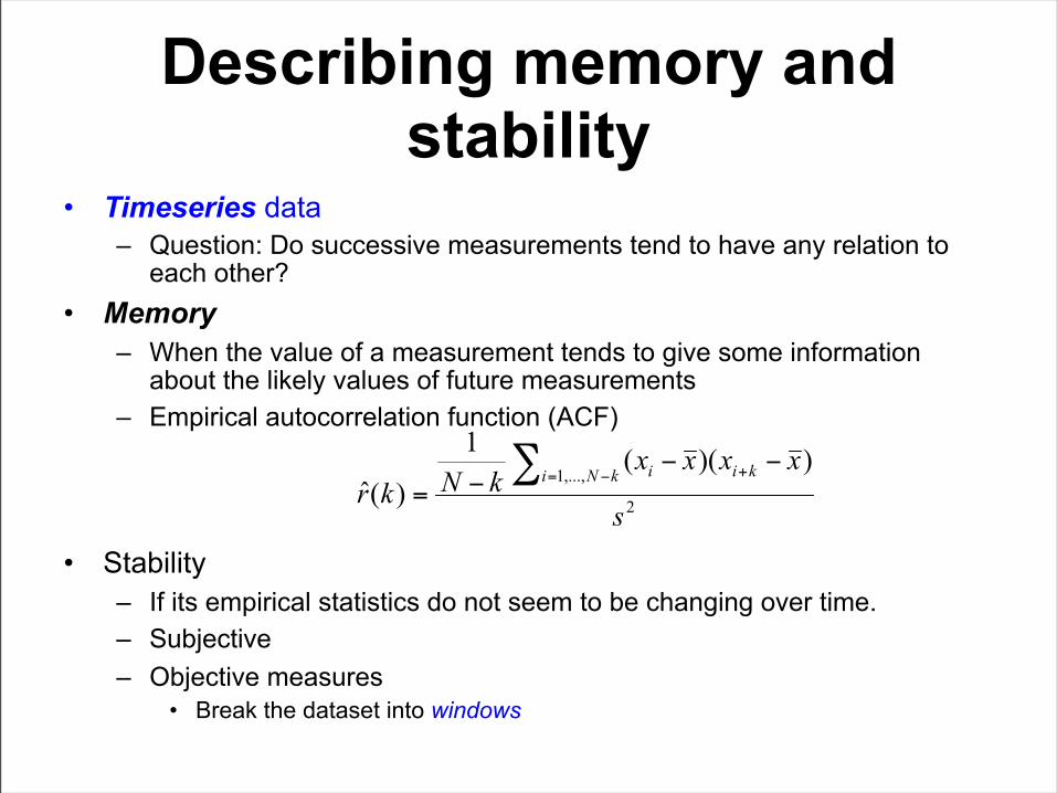
Describing memory and stability

• Timeseries data– Question: Do successive measurements tend to have any relation to

each other?• Memory

– When the value of a measurement tends to give some information about the likely values of future measurements

– Empirical autocorrelation function (ACF)

• Stability– If its empirical statistics do not seem to be changing over time.– Subjective– Objective measures

• Break the dataset into windows

Special issues• High variability (Numeric data distribution)

– Traditional statistical methods focuses on low or moderate variability of the data, e.g. Normal distribution

– Internet data shows high variability• It consists of many small values mixed with a small number of large

value• A significant fraction of the data may fall many standard deviations

from the mean• Empirical distribution is highly skewed, and empirical mean and

variance are strongly affected by the rare, large observations• It may be modeled with a subexponential or heavy tailed distribution• Mean and variance are not good metrics for high variability data,

while quantiles and the empirical distribution are better, e.g. empirical CCDF on log-log axes for long-tailed distribution

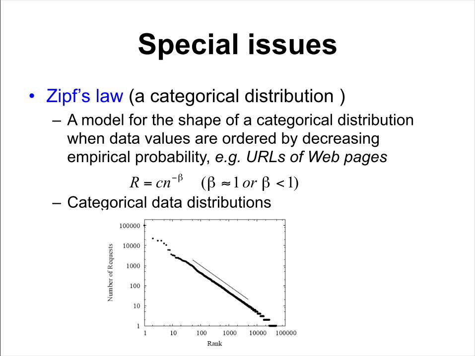
Special issues• Zipf’s law (a categorical distribution )

– A model for the shape of a categorical distribution when data values are ordered by decreasing empirical probability, e.g. URLs of Web pages

– Categorical data distributions

Graphs and Topology

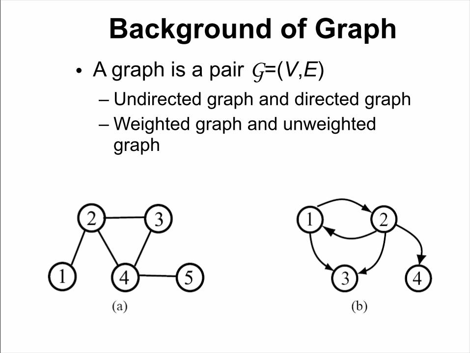
Background of Graph• A graph is a pair G=(V,E)

– Undirected graph and directed graph– Weighted graph and unweighted

graph

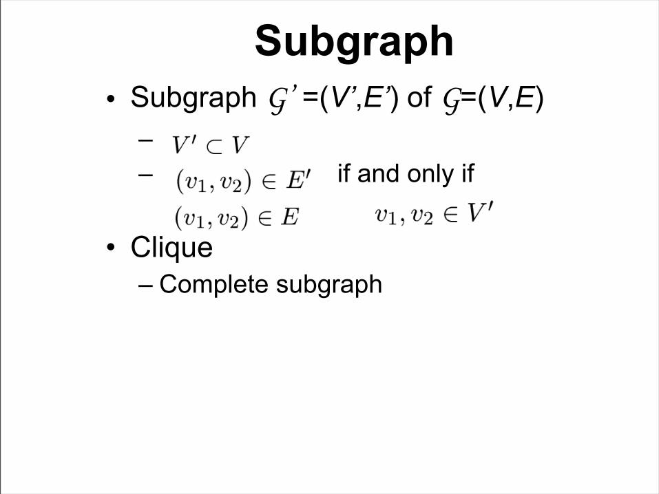
Subgraph• Subgraph G’ =(V’,E’) of G=(V,E)

– – if and only if and

• Clique– Complete subgraph

a b

c

d

e

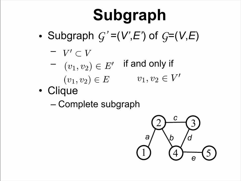
Subgraph• Subgraph G’ =(V’,E’) of G=(V,E)

– – if and only if and

• Clique– Complete subgraph

a b

c

d

e

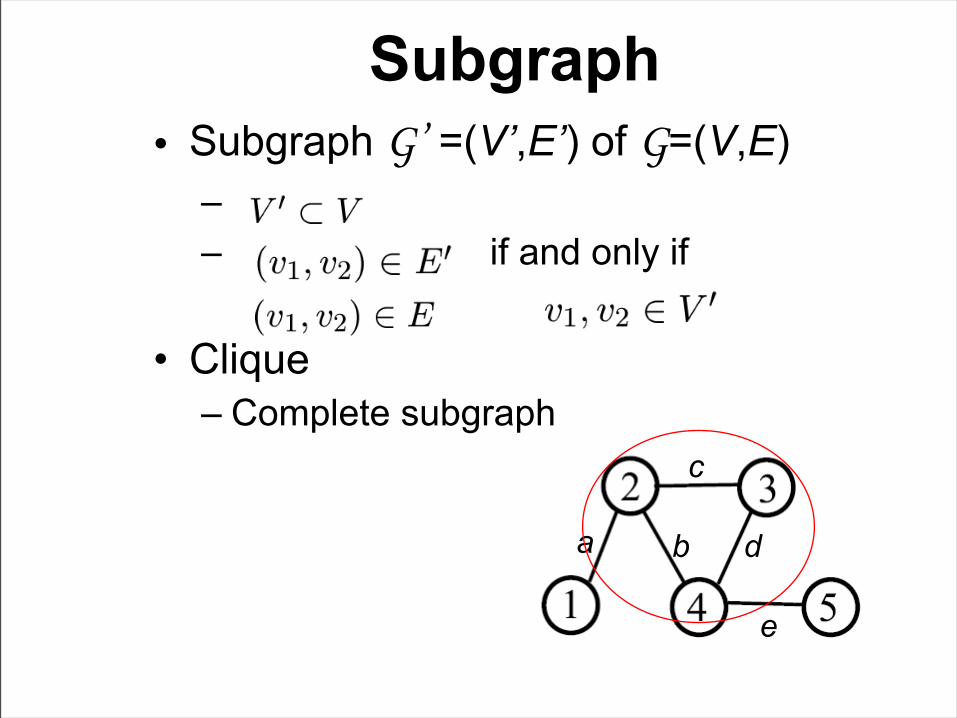
Subgraph• Subgraph G’ =(V’,E’) of G=(V,E)

– – if and only if and

• Clique– Complete subgraph

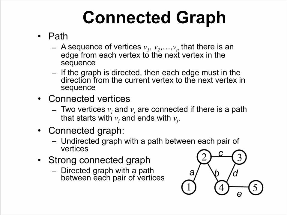
Connected Graph• Path

– A sequence of vertices v1, v2,…,vn that there is an edge from each vertex to the next vertex in the sequence

– If the graph is directed, then each edge must in the direction from the current vertex to the next vertex in sequence

• Connected vertices– Two vertices vi and vj are connected if there is a path

that starts with vi and ends with vj.• Connected graph:

– Undirected graph with a path between each pair of vertices

• Strong connected graph– Directed graph with a path

between each pair of vertices a b

c

d

e

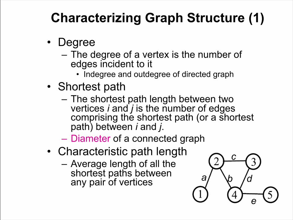
Characterizing Graph Structure (1)

• Degree– The degree of a vertex is the number of

edges incident to it• Indegree and outdegree of directed graph

• Shortest path– The shortest path length between two

vertices i and j is the number of edges comprising the shortest path (or a shortest path) between i and j.

– Diameter of a connected graph• Characteristic path length

– Average length of all the shortest paths between any pair of vertices a b

c

d

e

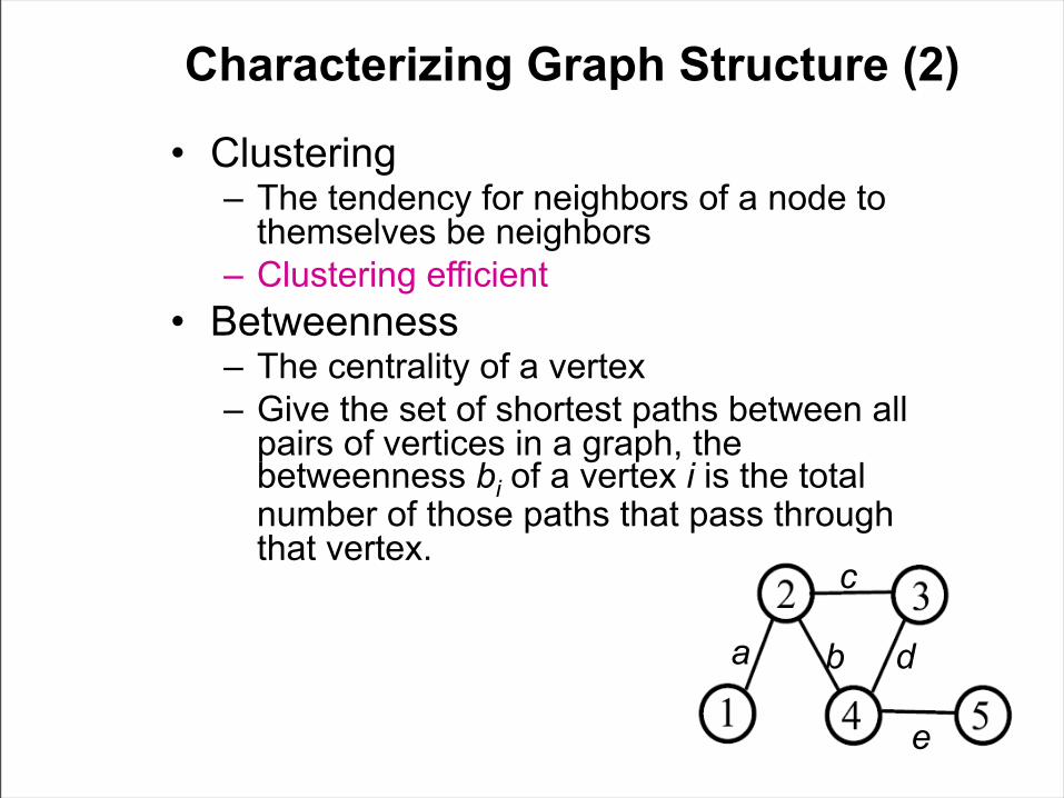
Characterizing Graph Structure (2)

• Clustering– The tendency for neighbors of a node to

themselves be neighbors– Clustering efficient

• Betweenness– The centrality of a vertex– Give the set of shortest paths between all

pairs of vertices in a graph, the betweenness bi of a vertex i is the total number of those paths that pass through that vertex.

a b

c

d

e

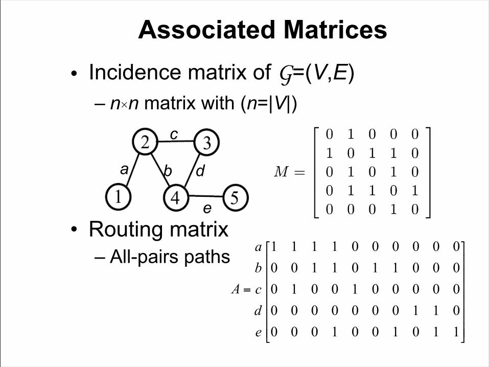
Associated Matrices• Incidence matrix of G=(V,E)

– n×n matrix with (n=|V|)

• Routing matrix– All-pairs paths

a b

c

d

e

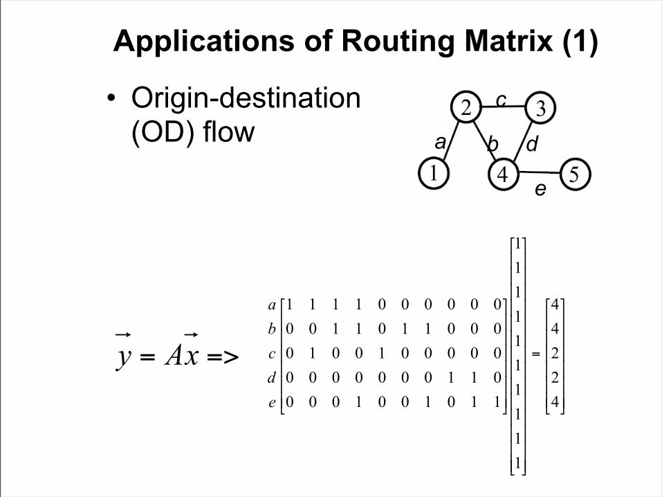
Applications of Routing Matrix (1)

• Origin-destination (OD) flow a b

c

d

e

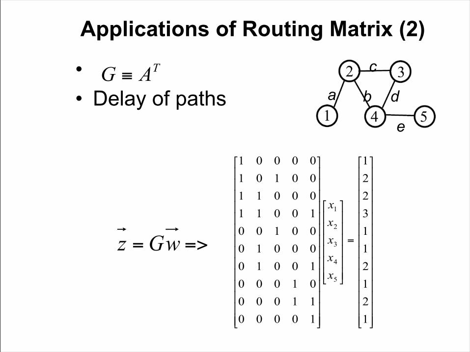
Applications of Routing Matrix (2)

• • Delay of paths a b

c

d

e

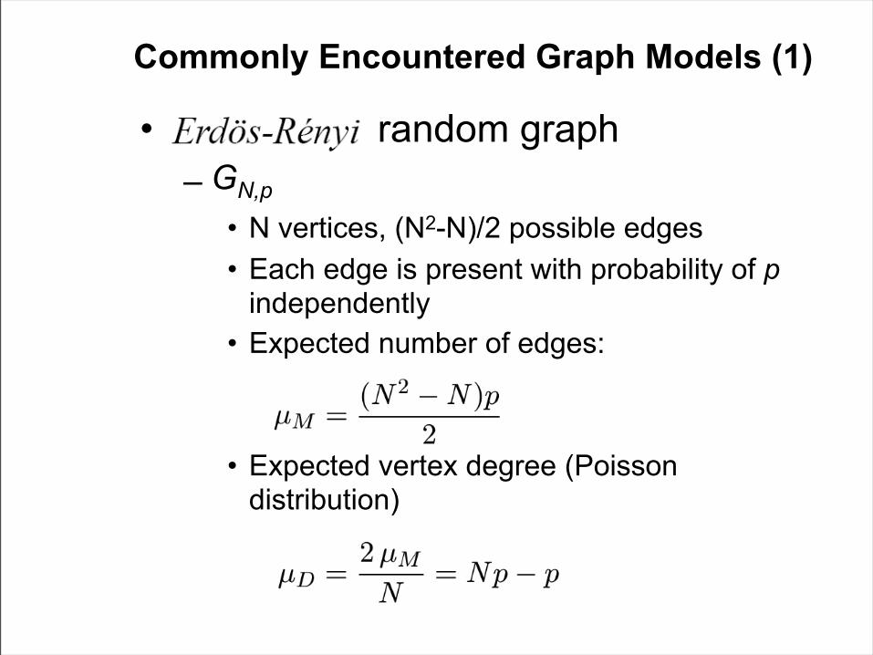
Commonly Encountered Graph Models (1)

• random graph– GN,p

• N vertices, (N2-N)/2 possible edges• Each edge is present with probability of p

independently• Expected number of edges:

• Expected vertex degree (Poisson distribution)

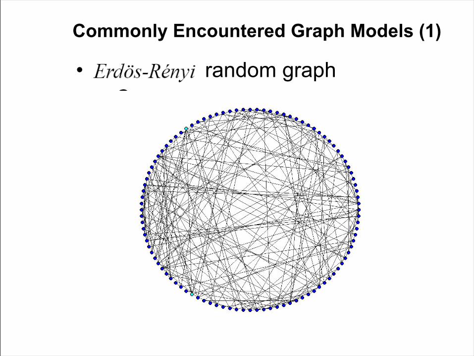
Commonly Encountered Graph Models (1)

• random graph– GN,p

• N vertices, (N2-N)/2 possible edges• Each edge is present with probability of p

independently• Expected number of edges:

• Expected vertex degree (Poisson distribution)

Commonly Encountered Graph Models (2)

• Generalized random graph– Given fixed degree sequence {di, i=1,…,N}

– Each degree di is assigned to one of the N vertices

– Edge are constructed randomly to satisfy the degree of each vertex

– Self-loop and duplicate links may occur

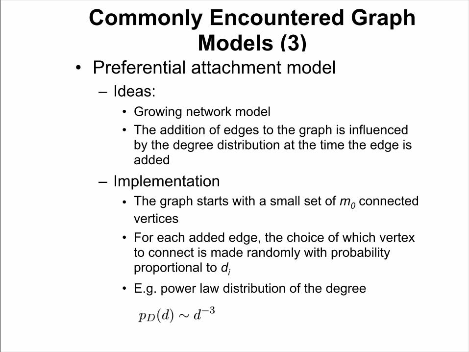
Commonly Encountered Graph Models (3)

• Preferential attachment model– Ideas:

• Growing network model• The addition of edges to the graph is influenced

by the degree distribution at the time the edge is added

– Implementation• The graph starts with a small set of m0 connected

vertices• For each added edge, the choice of which vertex

to connect is made randomly with probability proportional to di

• E.g. power law distribution of the degree

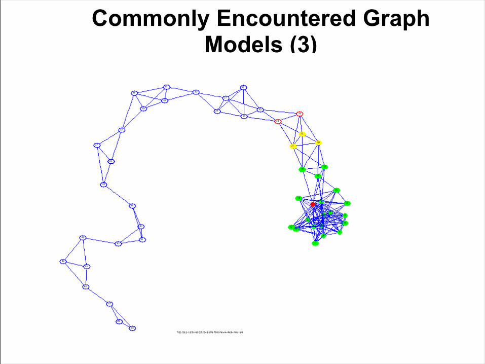
Commonly Encountered Graph Models (3)

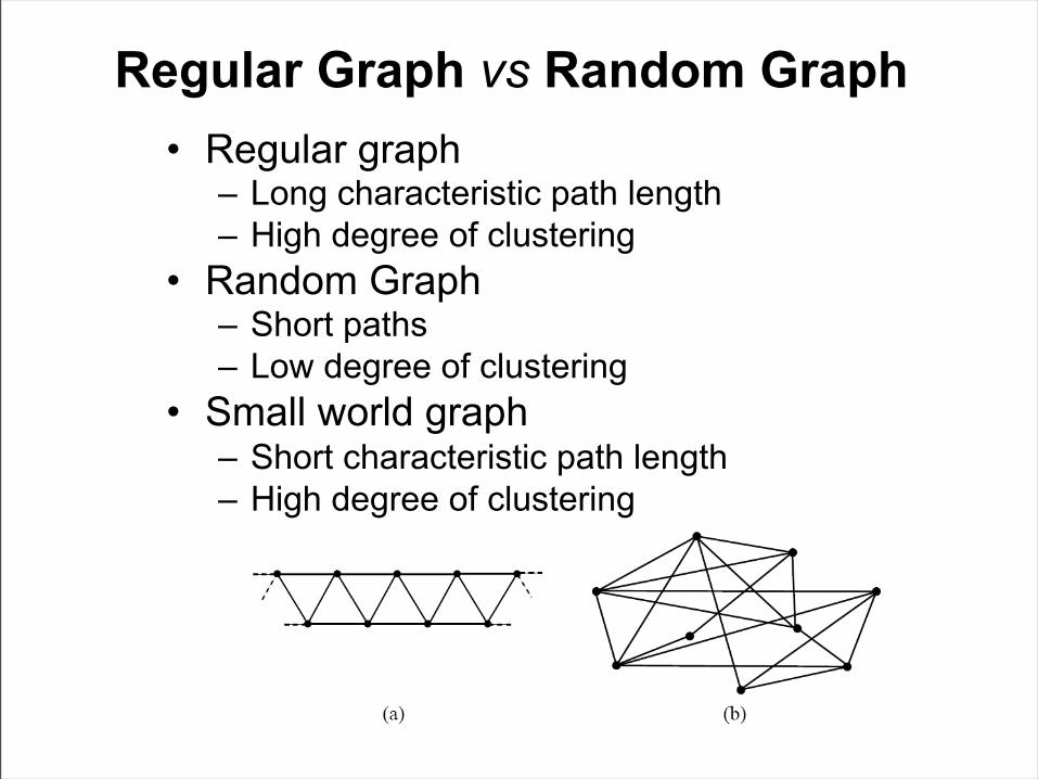
Regular Graph vs Random Graph• Regular graph

– Long characteristic path length– High degree of clustering

• Random Graph– Short paths– Low degree of clustering

• Small world graph– Short characteristic path length– High degree of clustering

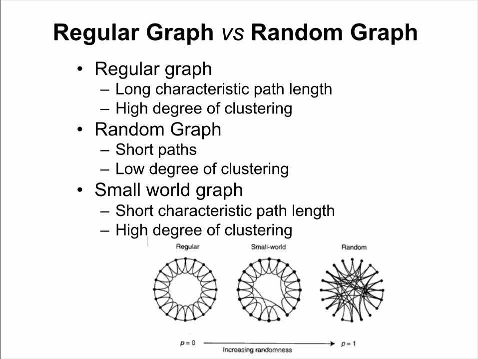
Regular Graph vs Random Graph• Regular graph

– Long characteristic path length– High degree of clustering

• Random Graph– Short paths– Low degree of clustering

• Small world graph– Short characteristic path length– High degree of clustering

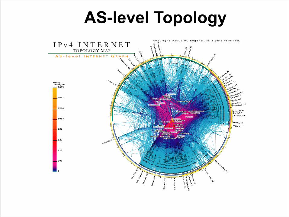
AS-level Topology

AS-level Topology

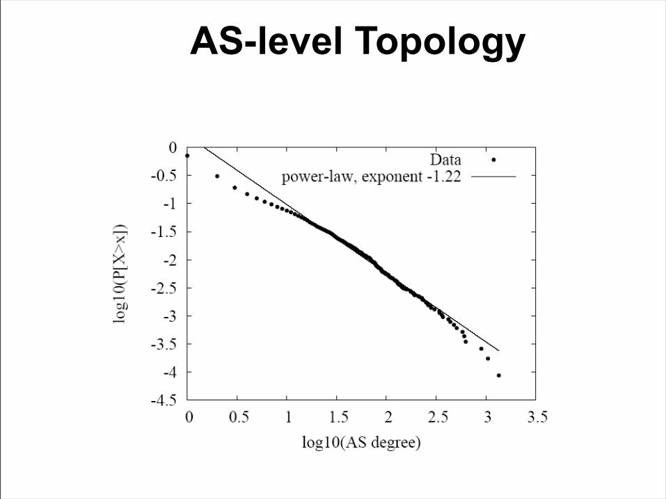
AS-level Topology• High variability in degree distribution

– Some ASes are very highly connected• Different ASes have dramatically different roles in

the network• Node degree seems to be highly correlated with

AS size

– Generative models of AS graph• “Rich get richer” model• Newly added nodes connect to existing nodes in

a way that tends to simultaneously minimize the physical length of the new connection, as well as the average number of hops to other nodes

• New ASes appear at an exponentially increasing rate, and each AS grows exponentially as well

AS Graph Is Small World • AS graph taken in Jan 2002

containing 12,709 ASes and 27,384 edges– Average path length is 3.6– Clustering coefficient is 0.46 (0.0014

in random graph)– It appears that individual clusters can

contain ASes with similar geographic location or business interests

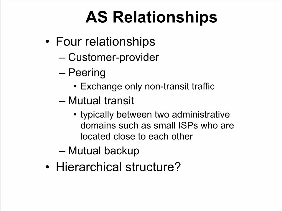
AS Relationships• Four relationships

– Customer-provider– Peering

• Exchange only non-transit traffic– Mutual transit

• typically between two administrative domains such as small ISPs who are located close to each other

– Mutual backup• Hierarchical structure?

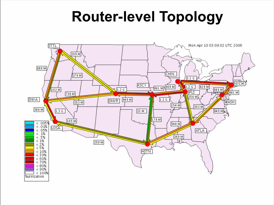
Router-level Topology

Router-level Topology• High variability in degree distribution

– Impossible to obtain a complete Internet topology– Most nodes have degree less than 5 but some can

have degrees greater than 100• High degree nodes tend to appear close to the network

edge• Network cores are more likely to be meshes

– Sampling bias (Mercator and Rocketful)• Proactive measurement (Passive measurement for AS

graph)• Nodes and links closest to the sources are explored

much more thoroughly • Artificially increase the proportion of low-degree nodes

in the sampled graph

• Path properties– Average length around 16, rare paths longer than 30

hops– Path inflation

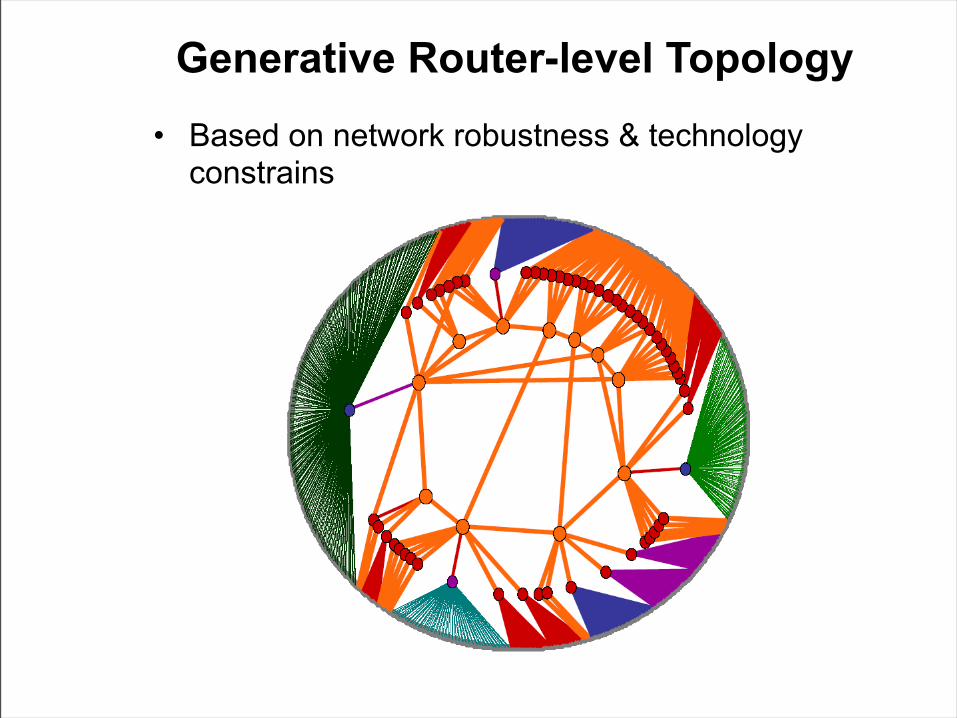
Generative Router-level Topology• Based on network robustness & technology

constrains

Dynamic Aspects of Topology

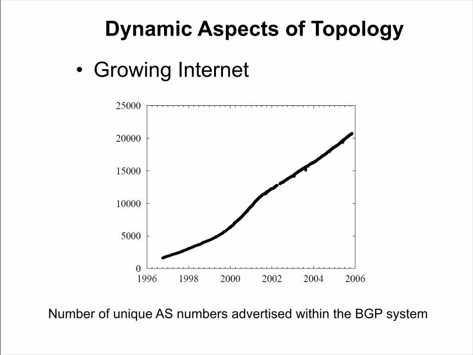
• Growing Internet

Number of unique AS numbers advertised within the BGP system

Dynamic Aspects of Topology• Difficult to measure the number of

routers– DNS is decentralized– Router-level graph changes rapidly

• Difficult measurement on endsystems– Intermittent connection– Network Address Translation (NAT)– No single centralized host registry

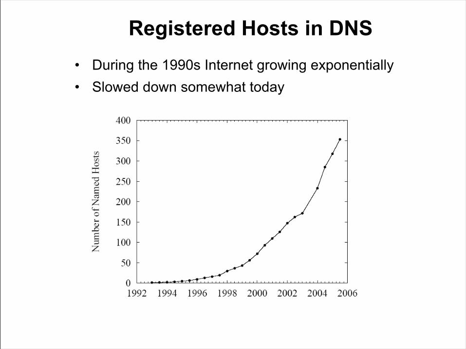
Registered Hosts in DNS• During the 1990s Internet growing exponentially• Slowed down somewhat today

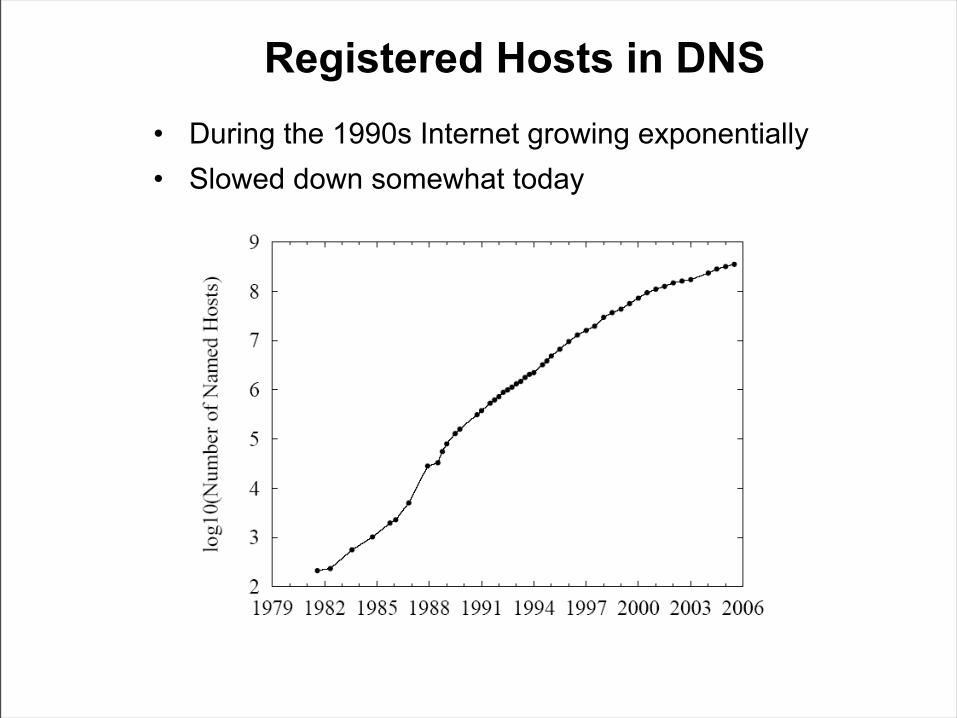
Registered Hosts in DNS• During the 1990s Internet growing exponentially• Slowed down somewhat today

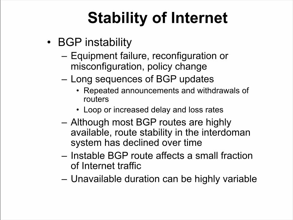
Stability of Internet• BGP instability

– Equipment failure, reconfiguration or misconfiguration, policy change

– Long sequences of BGP updates• Repeated announcements and withdrawals of

routers• Loop or increased delay and loss rates

– Although most BGP routes are highly available, route stability in the interdoman system has declined over time

– Instable BGP route affects a small fraction of Internet traffic

– Unavailable duration can be highly variable

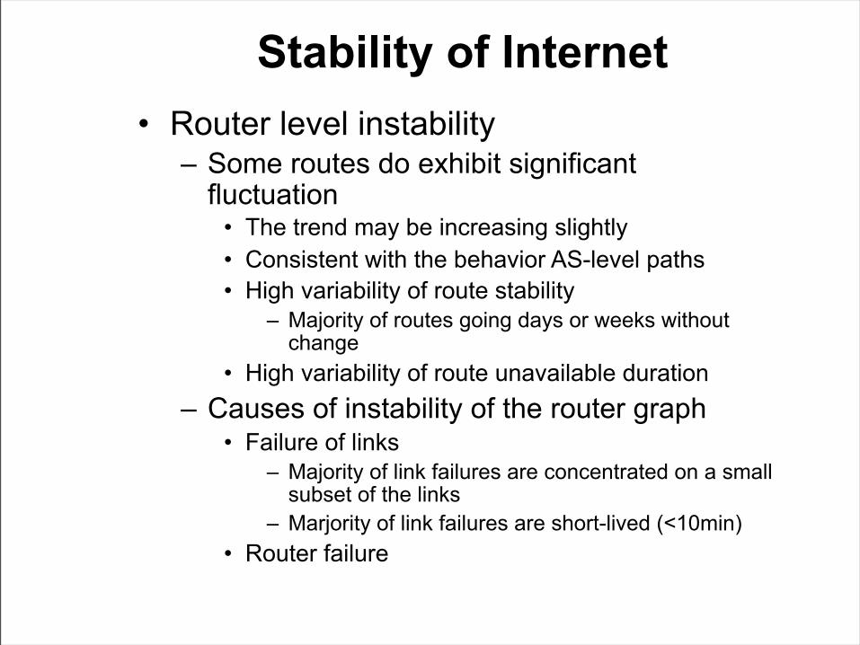
Stability of Internet• Router level instability

– Some routes do exhibit significant fluctuation

• The trend may be increasing slightly• Consistent with the behavior AS-level paths• High variability of route stability

– Majority of routes going days or weeks without change

• High variability of route unavailable duration– Causes of instability of the router graph

• Failure of links– Majority of link failures are concentrated on a small

subset of the links– Marjority of link failures are short-lived (<10min)

• Router failure

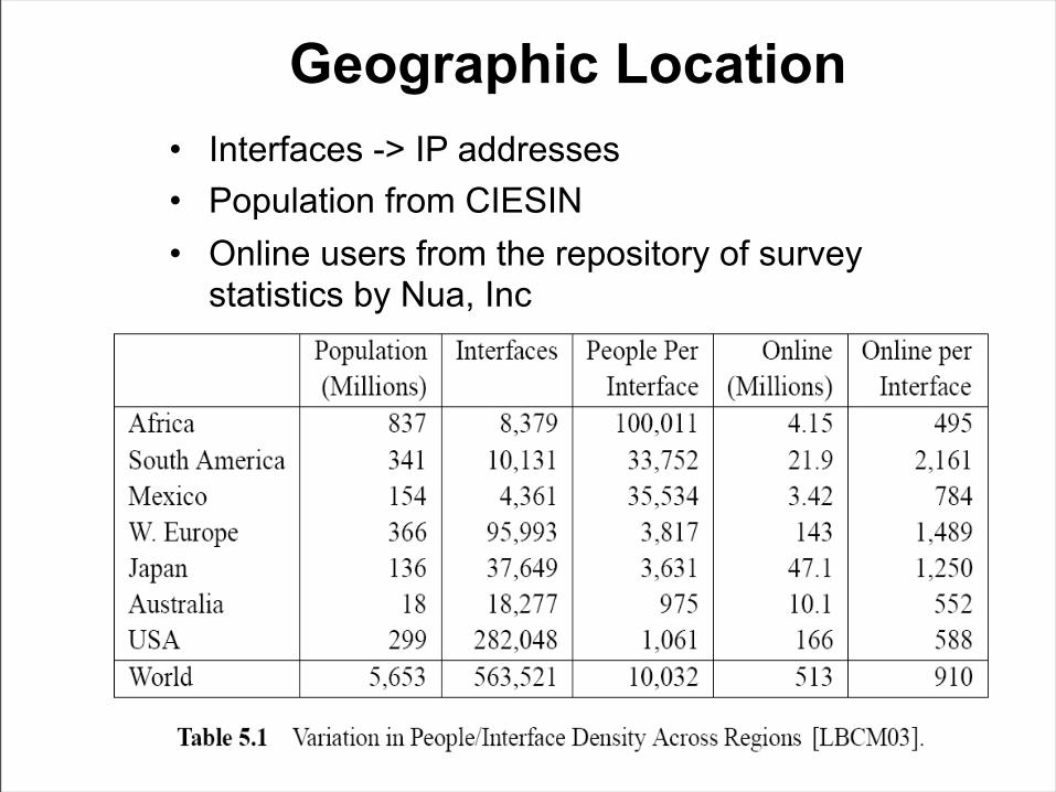
Geographic Location• Interfaces -> IP addresses• Population from CIESIN• Online users from the repository of survey

statistics by Nua, Inc

64

Measurement and Modeling

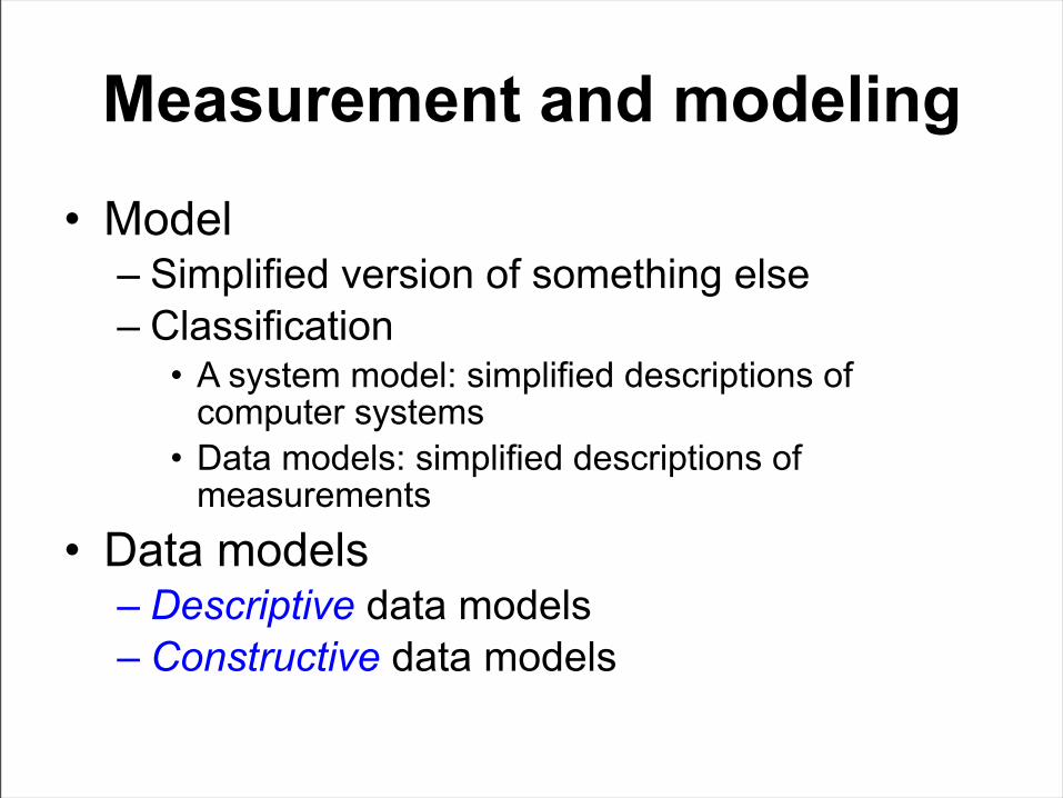
Measurement and modeling

• Model– Simplified version of something else– Classification

• A system model: simplified descriptions of computer systems

• Data models: simplified descriptions of measurements

• Data models– Descriptive data models– Constructive data models

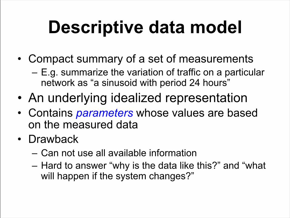
Descriptive data model• Compact summary of a set of measurements

– E.g. summarize the variation of traffic on a particular network as “a sinusoid with period 24 hours”

• An underlying idealized representation• Contains parameters whose values are based

on the measured data• Drawback

– Can not use all available information– Hard to answer “why is the data like this?” and “what

will happen if the system changes?”

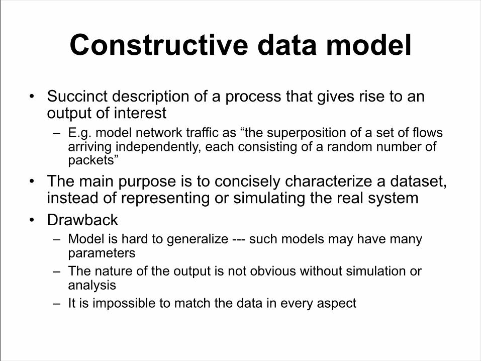
Constructive data model• Succinct description of a process that gives rise to an

output of interest– E.g. model network traffic as “the superposition of a set of flows

arriving independently, each consisting of a random number of packets”

• The main purpose is to concisely characterize a dataset, instead of representing or simulating the real system

• Drawback– Model is hard to generalize --- such models may have many

parameters– The nature of the output is not obvious without simulation or

analysis– It is impossible to match the data in every aspect

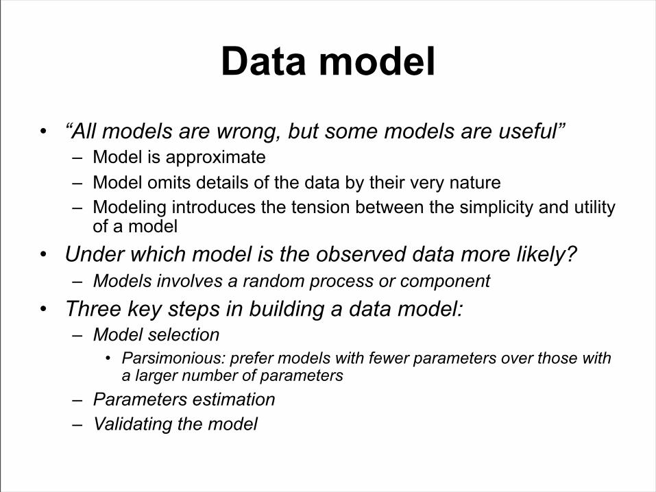
Data model• “All models are wrong, but some models are useful”

– Model is approximate– Model omits details of the data by their very nature– Modeling introduces the tension between the simplicity and utility

of a model• Under which model is the observed data more likely?

– Models involves a random process or component• Three key steps in building a data model:

– Model selection• Parsimonious: prefer models with fewer parameters over those with

a larger number of parameters– Parameters estimation– Validating the model

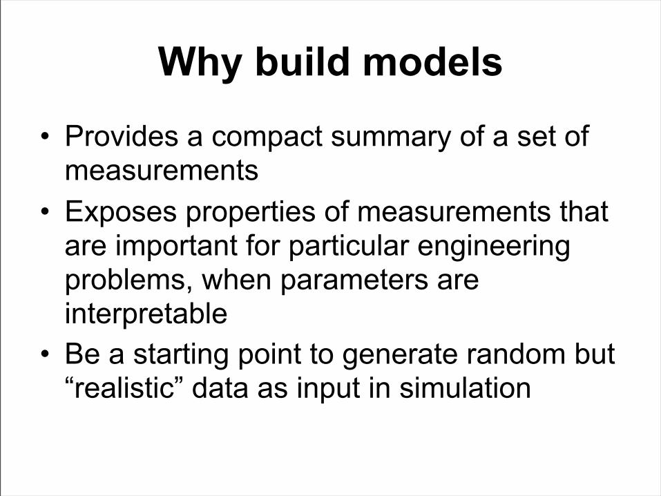
Why build models

• Provides a compact summary of a set of measurements

• Exposes properties of measurements that are important for particular engineering problems, when parameters are interpretable

• Be a starting point to generate random but “realistic” data as input in simulation

Probability models• Why use random models in the Internet?

– Fundamentally, the processes involved are random• The value is an immense number of particular system

properties that are far too tedious to specify

• Random models and real systems are very different things– It is important to distinguish between the properties of

a probabilistic model and the properties of real data.

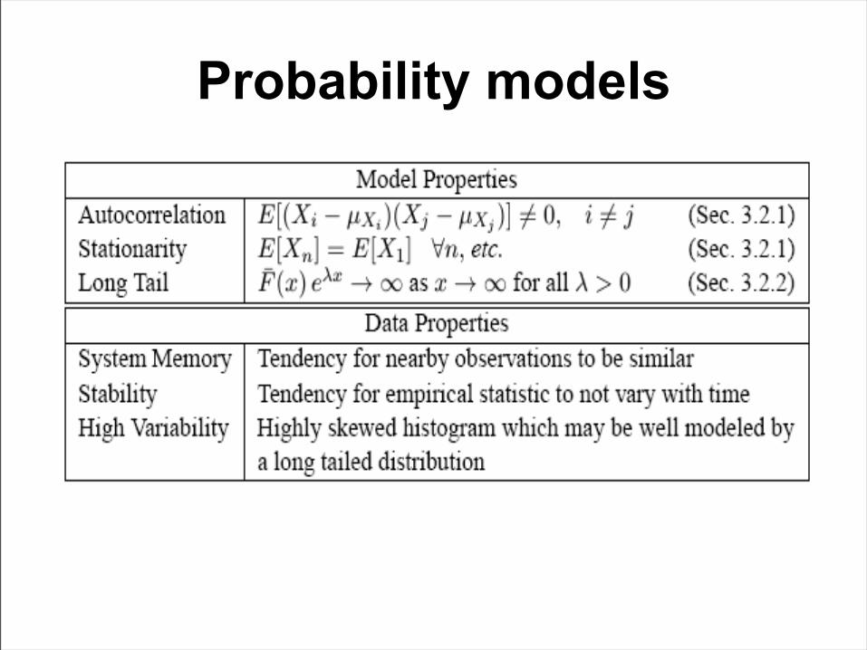
Probability models