Analyzing Mixed-Dyadic Data Using Structural Equation … · (e.g., Kenny & Ledermann, 2010). For example, individuals making up a traditional marital

This article was downloaded by: [University of California, Los Angeles (UCLA)]On: 16 April 2013, At: 06:10Publisher: RoutledgeInforma Ltd Registered in England and Wales Registered Number: 1072954 Registeredoffice: Mortimer House, 37-41 Mortimer Street, London W1T 3JH, UK

Structural Equation Modeling: AMultidisciplinary JournalPublication details, including instructions for authors andsubscription information:http://www.tandfonline.com/loi/hsem20

Analyzing Mixed-Dyadic Data UsingStructural Equation ModelsJames L. Peugh a , David DiLillo b & Jillian Panuzio ba Cincinnati Children's Hospital Medical Centerb University of Nebraska–LincolnVersion of record first published: 15 Apr 2013.

To cite this article: James L. Peugh , David DiLillo & Jillian Panuzio (2013): Analyzing Mixed-DyadicData Using Structural Equation Models, Structural Equation Modeling: A Multidisciplinary Journal,20:2, 314-337

To link to this article: http://dx.doi.org/10.1080/10705511.2013.769395

PLEASE SCROLL DOWN FOR ARTICLE

Full terms and conditions of use: http://www.tandfonline.com/page/terms-and-conditions

This article may be used for research, teaching, and private study purposes. Anysubstantial or systematic reproduction, redistribution, reselling, loan, sub-licensing,systematic supply, or distribution in any form to anyone is expressly forbidden.

The publisher does not give any warranty express or implied or make any representationthat the contents will be complete or accurate or up to date. The accuracy of anyinstructions, formulae, and drug doses should be independently verified with primarysources. The publisher shall not be liable for any loss, actions, claims, proceedings,demand, or costs or damages whatsoever or howsoever caused arising directly orindirectly in connection with or arising out of the use of this material.

http://www.tandfonline.com/loi/hsem20

http://dx.doi.org/10.1080/10705511.2013.769395

http://www.tandfonline.com/page/terms-and-conditions

Structural Equation Modeling, 20:314–337, 2013

Copyright © Taylor & Francis Group, LLC

ISSN: 1070-5511 print/1532-8007 online

DOI: 10.1080/10705511.2013.769395

TEACHER’S CORNER

Analyzing Mixed-Dyadic Data Using StructuralEquation Models

James L. Peugh,1 David DiLillo,2 and Jillian Panuzio2

1Cincinnati Children’s Hospital Medical Center2University of Nebraska–Lincoln

Mixed-dyadic data, collected from distinguishable (nonexchangeable) or indistinguishable (ex-

changeable) dyads, require statistical analysis techniques that model the variation within dyads

and between dyads appropriately. The purpose of this article is to provide a tutorial for perform-

ing structural equation modeling analyses of cross-sectional and longitudinal models for mixed

independent variable dyadic data, and to clarify questions regarding various dyadic data analysis

specifications that have not been addressed elsewhere. Artificially generated data similar to the

Newlywed Project and the Swedish Adoption Twin Study on Aging were used to illustrate analysis

models for distinguishable and indistinguishable dyads, respectively. Due to their widespread use

among applied researchers, the AMOS and Mplus statistical analysis software packages were used

to analyze the dyadic data structural equation models illustrated here. These analysis models are

presented in sufficient detail to allow researchers to perform these analyses using their preferred

statistical analysis software package.

Keywords: distinguishable, dyadic, exchangeable, indistinguishable, mixed

Applied researchers often pose empirical questions designed to test theories regarding individ-

uals, and subsequent data are typically analyzed assuming the responses from one participant

are independent of responses from all other participants. As such, applied researchers typically

identify the correct statistical analytic technique needed to answer such individualistic research

questions by considering (a) the type of research question posed (e.g., descriptive, comparative,

Correspondence should be addressed to James L. Peugh, Cincinnati Children’s Hospital & Medical Center, Behav-

ioral Medicine & Clinical Psychology, University of Cincinnati College of Medicine, Department of Pediatrics, Cin-

cinnati, OH 45229-3026. E-mail: [email protected]

314

Dow

nloa

ded

by [

Uni

vers

ity o

f C

alif

orni

a, L

os A

ngel

es (

UC

LA

)] a

t 06:

10 1

6 A

pril

2013

ANALYZING MIXED-DYADIC DATA IN SEM 315

or relationship), (b) the number of independent and dependent variables under consideration,

(c) the measurement scale of these variables, and (d) the sampling strategy used to obtain

the data. However, researchers also investigate questions designed to clarify how individuals

interact, and a dyad is defined as an interactive relationship between a pair of individuals (e.g.,

dating or married couples, monozygotic or dizygotic twins, or employer–employee, doctor–

patient, or parent–child relationships). If data were collected from dyadic relationships, three

additional considerations need to be addressed before the correct statistical analysis technique

can be identified and applied: dependence, distinguishability, and the type of dyadic variables

to be analyzed.

Dyadic dependence refers to the fact that the variable scores collected from individuals

interacting within dyads are not independent, but are likely to be more correlated than scores

from individuals in different dyads (cf. Gonzalez & Griffin, 1999; Kenny, Kashy, & Bolger,

1998). Further, dependence in dyadic data takes two forms. Similar to traditional analysis

models (e.g., ordinary least squares [OLS] regression) that specify shared predictor and re-

sponse variable variation, intrapersonal (relationships of variable scores from the same person)

dyadic dependence refers to the variation in an individual’s predictor or covariate score that

is shared with the variance of his or her own response variable score. However, interpersonal

(relationships of variables from different persons) dyadic dependence refers to the variation in

an individual’s predictor or covariate score that is shared with the variation of the other dyad

member’s response variable score (cf. Kenny, 1996). Dependence is an important issue because

traditional analysis approaches that assume independence of individual scores, such as analysis

of variance and OLS regression, can produce biased parameter estimates and standard errors if

applied incorrectly to dyadic data. A number of analytic techniques are available that estimate

the degree of dependence in dyadic data. Perhaps the most widely used approach is the intraclass

correlation (Gonzalez & Griffin, 2002; Kenny & Judd, 1996; McGraw & Wong, 1996), which

quantifies the proportion of response variable variability that is due to mean differences across

dyads. Dyadic dependence assessment is not reviewed here because researchers collect dyadic

data to answer dyadic research questions, the presence of dyadic dependence is to be expected,

and quantifying the amount of dependence present typically does not inform the research

question. Interested readers can consult Kenny, Kashy, and Cook (2006) for additional details

on assessing dependence. However, as shown in the analysis examples that follow, properly

specifying and modeling both the intrapersonal and interpersonal dependence is crucial to

dyadic data structural equation modeling (SEM) analysis.

This article illustrates the SEM analysis steps necessary to analyze mixed dyadic data

(i.e., data that vary both within a dyad and across dyads) sampled cross-sectionally and

longitudinally from either distinguishable or indistinguishable dyads. Dyadic distinguishability

refers to whether the two individuals comprising a dyad possess a distinctive characteristic that

can differentiate them in a manner that is relevant to the research question under investigation

(e.g., Kenny & Ledermann, 2010). For example, individuals making up a traditional marital

dyad could be identified by their designated gender value (e.g., gender: 1 D wives, 2 D

husbands) and could be considered distinguishable. By contrast, same-sex identical twins

are an example of dyads whose members could be considered indistinguishable because the

designation of “Person 1” and “Person 2” within each dyad would be arbitrary. Although

an empirical test of distinguishability is available (see Griffin & Gonzalez, 1995; Kenny &

Cook, 1999; Kenny et al., 2006), that test is not reviewed here. This article proceeds from the

Dow

nloa

ded

by [

Uni

vers

ity o

f C

alif

orni

a, L

os A

ngel

es (

UC

LA

)] a

t 06:

10 1

6 A

pril

2013

316 PEUGH, DiLILLO, PANUZIO

assumption that it is the research question under investigation, not the results of a statistical test,

that drives all research design and statistical analysis decisions involving dyad distinguishability.

To further clarify the distinguishability issue, consider an example of identical brother-sister

twins. If the research question under investigation was genetic in nature, this would suggest the

twins be treated as indistinguishable in the data analysis. However, several research questions

could be posed (e.g., skill level) that would suggest the twins be treated as distinguishable in

the data analysis. The key point to be made regarding the issue of dyad distinguishability is that

the question is not whether any variable exists on which dyads under consideration could be

rendered distinguishable or indistinguishable, but whether the variables that are crucial to the

theory being tested by the research question under investigation suggest the dyads be treated

as distinguishable or indistinguishable in the data analysis.

GOALS OF THIS ARTICLE

Artificially generated data consistent with the mean structures and covariance matrices of

both the Newlywed Project (DiLillo et al., 2009) and the Swedish Adoption Twin Study

on Aging (SATSA; Pedersen, 2004) were used to illustrate hypothetical analysis models

for distinguishable and indistinguishable dyads, respectively. The Newlywed Project involved

data collected from newlywed couples in 3 consecutive years to investigate the relationships

between various psychological phenomena and their subsequent impact on marital functioning.

The SATSA project involved data collected from twin pairs in 1987, 1990, and 1993 that

examined the relationships between measures of psychological functioning and quality of life.

As described later, it is further assumed that the research questions under investigation suggest

that the Newlywed marital couples be treated as distinguishable and the SATSA twins be

treated as indistinguishable in all of the dyadic data analysis examples.

The purpose of this article is to (a) show that several dyadic structural equation models

are available to model the intrapersonal and interpersonal dependence in mixed dyadic data

sampled from distinguishable or indistinguishable dyads; (b) provide specific analysis details

and explanations regarding how mixed dyadic data structural equation models are specified and

why certain modifications are needed for indistinguishable dyad structural equation models that

have not been addressed in other publications; (c) provide AMOS (Version 16) and Mplus (Ver-

sion 6.11; Muthén & Muthén, 1998–2010) examples for all dyadic analysis models described

here, as well as supplemental Microsoft Excel files designed to assist in the computation of

additional fit indexes for the indistinguishable dyad analysis models, in an Appendix available

at https://bmixythos.cchmc.org/xythoswfs/webui/_xy-476611_1-t_AXKarXYG; and (d) provide

descriptions of the analysis models used here in sufficient detail to allow researchers to apply

these models using the statistical analysis software package of their choice. For all dyadic data

analysis models shown here, the distinguishable dyad analysis models are described first so

that the model specification alterations needed to analyze data from indistinguishable dyads

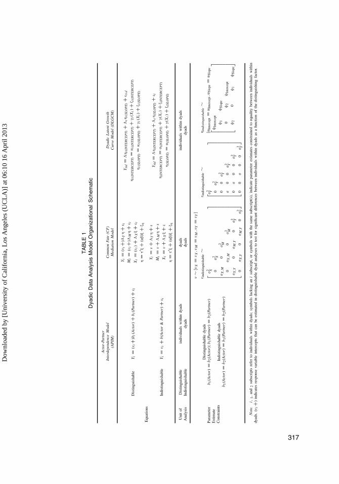
with the same analysis model are more clearly presented. Further, Table 1 presents an overview

of the dyadic data analysis model examples presented, their respective linear model equations,

the research questions addressed, and the parameter estimate constraints involved with each.

Finally, as demonstrated in all example analyses, the research question under investigation and

the distinguishability decision together dictate the dyadic structural equation model needed

Dow

nloa

ded

by [

Uni

vers

ity o

f C

alif

orni

a, L

os A

ngel

es (

UC

LA

)] a

t 06:

10 1

6 A

pril

2013

TA

BLE

1

Dyadic

Data

Analy

sis

Model

Org

aniz

ationa

lS

chem

atic

Act

or-

Part

ner

Inte

rdep

enden

ceM

odel

(AP

IM)

Com

mon

Fate

(CF

)

Med

iati

on

Model

Dya

dic

Late

nt

Gro

wth

Curv

eM

odel

(DL

GC

M)

Dis

tinguis

hab

leY

iD

.viC

/bi.A

ctor/

Cb

i.P

art

ner

/C

© i

Yi

D.v

iC

/ƒY

˜C

© i

Mi

D.v

iC

/ƒM

˜C

© i

Xi

D.v

i/

Cƒ

XŸ

C© i

˜D

£0 Ÿ

C.’

“/Ÿ

C— ˜

Yti

dD

ƒ˜

i.IN

TE

RC

EP

T/

Cƒ

t˜

i.SL

OP

E/

C© t

id

˜i.

INT

ER

CE

PT/

D’

i.IN

TE

RC

EP

T/

C”

i.X

i/

C— i

.IN

TE

RC

EP

T/

˜i.

SL

OP

E/

D’

i.SL

OP

E/

C”

i.X

i/

C— i

.SL

OP

E/

Equat

ions

Indis

tinguis

hab

leY

iD

vi

Cb

.Act

or

&P

art

ner

/C

© i

Yi

Dv

Cƒ

Y˜

C©

Mi

Dv

Cƒ

M˜

C©

Xi

Dv

Cƒ

XŸ

C©

˜D

£0 Ÿ

C.’

“/Ÿ

C— ˜

Yti

dD

ƒ˜

.IN

TE

RC

EP

T/

Cƒ

t˜

.SL

OP

E/

C© i

˜.I

NT

ER

CE

PT/

D’

.IN

TE

RC

EP

T/

C”.X

i/

C— .

INT

ER

CE

PT/

˜.S

LO

PE

/D

’.S

LO

PE

/C

”.X

i/

C— .

SL

OP

E/

Unit

of

Anal

ysi

s

Dis

tinguis

hab

le

Indis

tinguis

hab

le

indiv

idual

sw

ithin

dyad

s

dyad

s

dyad

s

dyad

s

indiv

idual

sw

ithin

dyad

s

dyad

s

Par

amet

er

Est

imat

e

Const

rain

ts

Dis

tinguis

hab

ledyad

s

b1.A

ctor/

Db

2.A

ctor/

Ib

1.P

art

ner

/D

b2.P

art

ner

/

Indis

tinguis

hab

ledyad

s

b1.A

ctor/

Db

2.A

ctor/

Db

1.P

art

ner

/D

b2.P

art

ner

/

v�

ŒvX

Dv

X;v

MD

vM

;vY

Dv

Y�

© indis

tinguis

hab

le�

2 6 6 6 6 6 6 6 6 4

¢2 X 0

¢2 X

¢X

;M0

¢2 M

0¢

X;M

0¢

2 M

¢X

;Y0

¢M

;Y0

¢2 Y

0¢

X;Y

0¢

M;Y

0¢

2 Y

3 7 7 7 7 7 7 7 7 5

© indis

tinguis

hab

le�

2 6 6 6 6 6 6 6 6 4

¢2 Y 0

¢2 Y

00

¢2 Y

¢0

0¢

2 Y

0¢

00

¢2 Y

00

¢0

0¢

2 Y

3 7 7 7 7 7 7 7 7 5

˜in

dis

tinguis

hable

�

Œ’In

terc

ept

D’

Inte

rcep

t;’

Slo

pe

D’

Slo

pe

2 6 6 6 6 4

§In

terc

ept

§1

§S

lope

0§

2§

Inte

rcep

t

§2

0§

1§

Slo

pe

3 7 7 7 7 5

Note

.i,

1,

and

2su

bsc

ripts

refe

rto

indiv

idual

sw

ithin

dyad

s;sy

mbols

lack

ing

ani

subsc

ript,

or

sym

bols

wit

hth

esa

me

subsc

ript(

s),

indic

ate

par

amet

eres

tim

ates

const

rain

edto

equal

ity

bet

wee

nin

div

idual

sw

ithin

dyad

s..v

iC

/in

dic

ates

resp

onse

vari

able

inte

rcep

tsth

atca

nbe

esti

mat

edin

dis

tinguis

hab

ledyad

anal

yse

sto

test

for

signifi

cant

dif

fere

nce

sbet

wee

nin

div

idual

sw

ithin

dyad

sas

afu

nct

ion

of

the

dis

tinguis

hin

gfa

ctor.

317

Dow

nloa

ded

by [

Uni

vers

ity o

f C

alif

orni

a, L

os A

ngel

es (

UC

LA

)] a

t 06:

10 1

6 A

pril

2013


FIGURE 1 Distinguishable dyad actor–partner interdependence (APIM) analysis model. **p < :01.

and how the intrapersonal and interpersonal dyadic dependence should be specified within the

model.

CROSS-SECTIONAL DYADIC DATA ANALYSES

Researchers collect cross-sectional data from dyads to answer research questions involving

interpersonal dynamics, such as whether the predictor variable score of the first dyad member

.X1/ is significantly related to their own response variable .Y1/ score (i.e., X1 ! Y1; an

intrapersonal or “actor” effect), and if the predictor variable score of the first dyad member is

significantly related to the response variable score of the second dyad member (i.e., X1 ! Y2;

an interpersonal or “partner” effect; Cook & Kenny, 2005; Furman & Simon, 2006; Kenny,

1996). A traditional SEM analysis model used to answer research questions involving dyadic

intrapersonal and interpersonal relationship patterns is the actor–partner interdependence model

(APIM; cf. Kenny, 1996). An example APIM that investigates the intrapersonal and inter-

personal relationships between childhood psychological maltreatment and subsequent marital

satisfaction among newlywed couples is shown in Figure 1.

Distinguishable Dyads

The APIM shown in Figure 1 estimates (a) predictor variable (psychological maltreatment)

Dow

nloa

ded

by [

Uni

vers

ity o

f C

alif

orni

a, L

os A

ngel

es (

UC

LA

)] a

t 06:

10 1

6 A

pril

2013


TABLE 2

Actor–Partner Interdependence Model Fit Statistics

Distinguishable Dyads Indistinguishable Dyads

Null

Model

Analysis

Model, Initial

Analysis

Model, Final

Saturated

Model

Null

Model

Analysis

Model

Saturated

Model

¦2 387.38 13.66 4.91 0 65.97 10.97 9.99

df 6 3 2 0 10 3 6LogL �4,028.83 �3,841.97 �3,837.60 �3,835.14 �3,831.02 �3,803.52 �3,803.03

means, (b) response variable (marital satisfaction) intercepts, (c) predictor variable variances,

(d) response variable residual .e/ variances, (e) a predictor variable covariance (Cx), (f) a

residuals covariance (Cy), (g) actor (bACTOR) effects, and (h) partner (bPARTNER) effects. In-

trapersonal dyadic dependence is modeled through the estimation of actor effects (bACTOR);

interpersonal dyadic dependence is modeled through the estimation of partner effects (bPARTNER)

and covariances (Cx and Cy). Estimating each of these parameters separately for the two dyad

members results in a saturated model (in more complex analyses, the unconstrained model

might not be saturated). The goal of an APIM analysis in the distinguishable dyad case is

to test the fit of more parsimonious models that constrain actor and partner effect estimates.

For example, two of the more common constraint patterns in the distinguishable case involve

a model that constrains actor effects (e.g., bACTOR;Wives D bACTOR;Husbands) and partner effects

(e.g., bPARTNER;Wives D bPARTNER;Husbands) separately to equality (i.e., where bACTOR ¤ bPARTNER),

and a model constraining all four effects (e.g., bACTOR;Wives D bACTOR;Husbands D bPARTNER;Wives D

bPARTNER;Husbands/ to equality. These equality constraints allow testing for significant differences

in actor and partner effects between distinguishable dyad members (Gonzalez & Griffin, 2001).

It is important to note that the standard null and saturated structural equation models are the

appropriate models with which to test the fit of an APIM with distinguishable dyads. However,

the definition and specification of the appropriate null and saturated models will differ for

indistinguishable dyad analyses, as shown in the subsequent sections.

Distinguishable APIM example. As an example, the APIM shown in Figure 1 was

estimated using the Newlywed Project data to quantify childhood psychological maltreatment

and subsequent marital satisfaction actor and partner effects, and to test for possible differences

in these effects between newlywed husbands and wives. As shown in the left panel of Table 2,

estimating an initial analysis model that constrained all four regression paths to equality resulted

in the following chi-square model fit index value: ¦23 D 13:66, p < :01 (not shown in Table 1:

comparative fit index [CFI] D .97, Tucker–Lewis Index [TLI] D .95, root mean square error of

approximation [RMSEA] D .09).1 Modification indexes showed that the husband actor effect

1This article used generated hypothetical data to demonstrate the procedures involved in various dyadic data

analyses using SEM, not to evaluate dyadic data analysis models. Model fit statistic values are presented “as is”; no

judgments as to the quality of the fit of the model to the data are made and no theoretical conclusions should be drawn

from the hypothetical results presented.

Dow

nloa

ded

by [

Uni

vers

ity o

f C

alif

orni

a, L

os A

ngel

es (

UC

LA

)] a

t 06:

10 1

6 A

pril

2013


path (bACTORWHusband) should be freed; estimating that final analysis model resulted in the follow-

ing chi-square model fit index value: ¦22 D 4:91, p > :05 (CFI D .99, TLI D .98, RMSEA D

.06). The final model parameter estimates are shown in Figure 1. As childhood psychological

maltreatment for either spouse increased, marital satisfaction significantly decreased for both

spouses, but this decrease was significantly greater for the relationship between husbands’

childhood maltreatment experiences and husbands’ marital satisfaction.

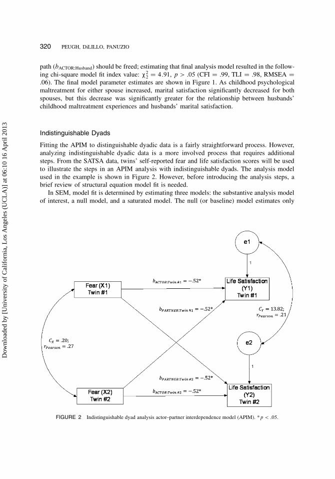
Indistinguishable Dyads

Fitting the APIM to distinguishable dyadic data is a fairly straightforward process. However,

analyzing indistinguishable dyadic data is a more involved process that requires additional

steps. From the SATSA data, twins’ self-reported fear and life satisfaction scores will be used

to illustrate the steps in an APIM analysis with indistinguishable dyads. The analysis model

used in the example is shown in Figure 2. However, before introducing the analysis steps, a

brief review of structural equation model fit is needed.

In SEM, model fit is determined by estimating three models: the substantive analysis model

of interest, a null model, and a saturated model. The null (or baseline) model estimates only

FIGURE 2 Indistinguishable dyad analysis actor–partner interdependence model (APIM). *p < :05.

Dow

nloa

ded

by [

Uni

vers

ity o

f C

alif

orni

a, L

os A

ngel

es (

UC

LA

)] a

t 06:

10 1

6 A

pril

2013


means and variances for each analysis variable, constrains all possible analysis variable covari-

ances to zero, and is considered the worst possible model to fit to a set of sample data.2 A satu-

rated model is defined as a model that freely estimates all analysis variable means, variances,

and covariances. The saturated model is considered the best fitting model possible, but is not

parsimonious and is seldom of interest to researchers. Together the null (worst fitting model

possible) and saturated (best fitting model possible) models provide a continuum within which

to evaluate the fit of the analysis model.

The proper chi-square model fit statistic for a substantive structural equation model is

obtained by subtracting the chi-square statistic for the saturated model from the chi-square

statistic for the analysis model. This chi-square difference value is then tested by referencing

it to a chi-square distribution at degrees of freedom equal to the difference in the number

of estimated parameters between the analysis and saturated models. However, the chi-square

statistic for a typical structural equation model is tested directly by referencing it to a chi-square

distribution at degrees of freedom equal to the degrees of freedom for the analysis model

because a typical saturated structural equation model has a chi-square statistic and degrees of

freedom that are both zero. This chi-square model fit statistic quantifies misspecification, or

the lack of fit of the analysis model to the sample data.

In addition to theoretical misspecification, indistinguishable dyad structural equation models

contain a second source of model misfit: arbitrary designation. Specifically, the designation

of Person 1 and Person 2 within each indistinguishable dyad would be arbitrary, but not

inconsequential. As demonstrated elsewhere (Woody & Sadler, 2005), reversing this arbitrary

Person 1/Person 2 designation for some, but not all, of the dyads in the sample data set can

notably alter the relationships among analysis variables. A method of removing this arbitrary

misfit, leaving only a quantification of analysis model misspecification, is needed to accurately

evaluate the fit of an APIM for indistinguishable dyads. As shown later, removing arbitrary

designation misfit involves the estimation of chi-square statistics and degrees of freedom for

null and analysis structural equation models in the usual fashion, but it also involves the

estimation of a special saturated model with a chi-square statistic and degrees of freedom that

are both nonzero. The term saturated is used throughout the article to maintain a consistency

with the dyadic literature even though the indistinguishable dyad saturated models shown here

are not saturated from the usual SEM perspective.

Specifically, in a typical structural equation model, estimating a saturated model involves

estimating all possible parameters for a set of data, which uses all available degrees of freedom

and results in a chi-square fit statistic value of zero. However, the appropriate saturated model

for indistinguishable dyads involves estimating all parameters that make logical sense, but

would not exhaust all degrees of freedom. Specifically, for APIMs, separate parameter estimates

for the two dyad members would not be needed for indistinguishable dyads because there

would be no theoretical reason to expect differences, and any observed differences would

be due to arbitrary designation. As a result, an indistinguishable dyad saturated (or I-SAT;

Olsen & Kenny, 2006) model is defined as a model that constrains the following six pairs of

2No consensus currently exists, either in the empirical literature or across statistical analysis software packages, as

to whether exogenous variable covariances should be estimated in a null model (see Widaman & Thompson, 2003).

For all null models used here (e.g., Figures 4, 8, and 11), all analysis variable covariances were manually fixed to zero

in Mplus and AMOS.

Dow

nloa

ded

by [

Uni

vers

ity o

f C

alif

orni

a, L

os A

ngel

es (

UC

LA

)] a

t 06:

10 1

6 A

pril

2013


parameter estimates (i.e., each element of the sample mean vector and covariance matrix) to

equality between Person 1 and Person 2: (a) predictor variable means, (b) predictor variable

variances, (c) intrapersonal covariances, (d) interpersonal covariances, (e) response variable

means, and (f) response variable variances, as shown in Figure 3. Notice in Figure 3 that the

model is saturated in the traditional sense; the model estimates all possible associations among

analysis variables. However, the degrees of freedom value for this model is not zero due to

the equality constraints imposed as a result of the arbitrary Person 1/Person 2 designation of

indistinguishable dyad members.

Several properties of the I-SAT model are noteworthy. If dyad members were perfectly

indistinguishable (i.e., if predictor and response variable means, variances, and covariances

each were equivalent between both dyad members), the I-SAT model chi-square fit statistic

would equal zero, the model would have six degrees of freedom due to the equality constraints,

and the model-reproduced covariance matrix would match the sample data covariance matrix

(Carey, 2005). Assuming that the dyads under investigation are not perfectly indistinguishable,

FIGURE 3 Indistinguishable dyad actor–partner interdependence model (APIM) saturated model: (a) predic-

tor variable means, (b) predictor variable variances, (c) intrapersonal covariances, (d) interpersonal covariances,

(e) response variable means, and (f) response variable variances constrained to equality. The two unlabeled

covariances on the left side of the model are freely estimated (i.e., not given a letter label) to model interpersonal

dyadic dependence.

Dow

nloa

ded

by [

Uni

vers

ity o

f C

alif

orni

a, L

os A

ngel

es (

UC

LA

)] a

t 06:

10 1

6 A

pril

2013


reversing the Person 1/Person 2 designation for some, but not all, of the dyads in the sample

data set would change the I-SAT model chi-square fit statistic value, but the model parameter

estimates would not change. This means that the I-SAT’s nonzero chi-square statistic value

quantifies arbitrary designation misfit only (Kenny et al., 2006; Olsen & Kenny, 2006).

Computing the proper chi-square model fit statistic for an indistinguishable dyad APIM

requires subtracting the chi-square fit statistic for the indistinguishable dyad saturated model

(Figure 3, which contains only arbitrary designation misfit) from the chi-square fit statistic for

the indistinguishable dyad analysis model (Figure 2, which contains both model misspecifi-

cation and arbitrary designation misfit), and testing the resulting chi-square difference value

(which now quantifies model misspecification only) by referencing a chi-square distribution

with degrees of freedom equal to the difference in the number of estimated parameters between

the analysis and saturated models. (Alternatively, the chi-square difference test can also be im-

plemented by subtracting the log-likelihood values of the two models rather than the chi-square

statistics.) Conceptually, the I-SAT model is the correct saturated model for indistinguishable

dyads just as an unconstrained APIM is the correct saturated model for distinguishable dyads

(Olsen & Kenny, 2006). Further, the I-SAT model serves as the best fitting indistinguishable

model against which to test substantive APIMs that contain additional parameter estimate

constraints.

Although most SEM analysis software packages provide analysis model and null model

chi-square statistics and degrees of freedom by default, neither are the appropriate statistics

for the purposes of computing additional SEM fit indexes, such as the CFI, TLI, and the

RMSEA, for indistinguishable dyad APIMs. Computing the correct fit indexes begins by

estimating the appropriate indistinguishable dyad baseline or null model, which can be done

by fixing all covariances in the indistinguishable dyad saturated model to zero. This results

in a model that estimates means and variances only, as shown in Figure 4. For fit index

computation purposes, the correct analysis model chi-square statistic and degrees of freedom

are obtained by subtracting the indistinguishable dyad saturated model (Figure 3) chi-square

statistic and degrees of freedom from the indistinguishable dyad analysis model (Figure 2)

chi-square statistic and degrees of freedom. Similarly, the appropriate chi-square statistic

and degrees of freedom for the null (or baseline) model for fit index computation purposes

involves subtracting the indistinguishable dyad saturated model (Figure 3) chi-square statistic

and degrees of freedom from the indistinguishable dyad null or baseline model (Figure 4)

chi-square statistic and degrees of freedom.

Indistinguishable APIM example. The APIM shown in Figure 2 was used to test for

differences in the actor and partner effects relating self-reported fear to life satisfaction among

pairs of twins. The right panel of Table 2 shows that estimating an analysis model that

constrained all four regression paths to equality resulted in the following chi-square model

fit index value: ¦23 D 10:97, p < :05 (not shown in Table 2: CFI D .74, TLI D .57,

RMSEA D .08). However, recall that this chi-square fit statistic contains both misspecification

and arbitrary designation misfit. Arbitrary designation misfit is removed by subtracting the

chi-square fit statistic of the saturated model from the chi-square fit statistic of the analysis

model .10:97 � 9:99 D 0:98/. This chi-square difference value is then tested at a chi-square

distribution equal to the difference in the number of parameters estimated between the two

models .6 � 3 D 3/. After arbitrary designation was removed, the analysis model showed

Dow

nloa

ded

by [

Uni

vers

ity o

f C

alif

orni

a, L

os A

ngel

es (

UC

LA

)] a

t 06:

10 1

6 A

pril

2013


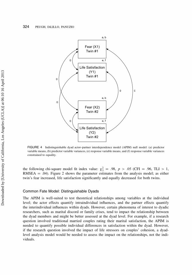
FIGURE 4 Indistinguishable dyad actor–partner interdependence model (APIM) null model: (a) predictor

variable means, (b) predictor variable variances, (e) response variable means, and (f) response variable variances

constrained to equality.

the following chi-square model fit index value: ¦23 D :98, p > :05 (CFI D .96, TLI > 1,

RMSEA D .04). Figure 2 shows the parameter estimates from the analysis model; as either

twin’s fear increased, life satisfaction significantly and equally decreased for both twins.

Common Fate Model: Distinguishable Dyads

The APIM is well-suited to test theoretical relationships among variables at the individual

level; the actor effects quantify intraindividual influences, and the partner effects quantify

the interindividual influences within dyads. However, certain phenomena of interest to dyadic

researchers, such as marital discord or family crises, tend to impact the relationship between

the dyad members and might be better assessed at the dyad level. For example, if a research

question involved traditional married couples rating their marital satisfaction, the APIM is

needed to quantify possible individual differences in satisfaction within the dyad. However,

if the research question involved the impact of life stressors on couples’ cohesion, a dyad-

level analysis model would be needed to assess the impact on the relationships, not the indi-

viduals.

Dow

nloa

ded

by [

Uni

vers

ity o

f C

alif

orni

a, L

os A

ngel

es (

UC

LA

)] a

t 06:

10 1

6 A

pril

2013


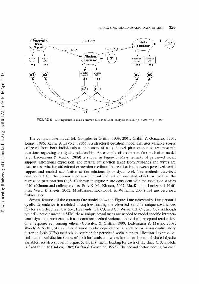
FIGURE 5 Distinguishable dyad common fate mediation analysis model. *p < :05. **p < :01.

The common fate model (cf. Gonzalez & Griffin, 1999, 2001; Griffin & Gonzalez, 1995;

Kenny, 1996; Kenny & LaVoie, 1985) is a structural equation model that uses variable scores

collected from both individuals as indicators of a dyad-level phenomenon to test research

questions regarding the dyadic relationship. An example of a common fate mediation model

(e.g., Ledermann & Macho, 2009) is shown in Figure 5. Measurements of perceived social

support, affectional expression, and marital satisfaction taken from husbands and wives are

used to test whether affectional expression mediates the relationship between perceived social

support and marital satisfaction at the relationship or dyad level. The methods described

here to test for the presence of a significant indirect or mediated effect, as well as the

regression path notation .’; “; £0/ shown in Figure 5, are consistent with the mediation studies

of MacKinnon and colleagues (see Fritz & MacKinnon, 2007; MacKinnon, Lockwood, Hoff-

man, West, & Sheets, 2002; MacKinnon, Lockwood, & Williams, 2004) and are described

further later.

Several features of the common fate model shown in Figure 5 are noteworthy. Intrapersonal

dyadic dependence is modeled through estimating the observed variable unique covariances

(C) for each dyad member (i.e., Husbands: C1, C3, and C5; Wives: C2, C4, and C6). Although

typically not estimated in SEM, these unique covariances are needed to model specific intraper-

sonal dyadic phenomena such as a common method variance, individual perceptual tendencies,

or a response set, among others (Gonzalez & Griffin, 1999; Ledermann & Macho, 2009;

Woody & Sadler, 2005). Interpersonal dyadic dependence is modeled by using confirmatory

factor analysis (CFA) methods to combine the perceived social support, affectional expression,

and marital satisfaction scores of both husbands and wives into three latent and shared dyadic

variables. As also shown in Figure 5, the first factor loading for each of the three CFA models

is fixed to unity (Bollen, 1989; Griffin & Gonzalez, 1995). The second factor loading for each

Dow

nloa

ded

by [

Uni

vers

ity o

f C

alif

orni

a, L

os A

ngel

es (

UC

LA

)] a

t 06:

10 1

6 A

pril

2013


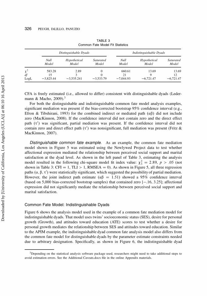
TABLE 3

Common Fate Model Fit Statistics


Null

Model

Hypothetical

Model

Saturated

Model

Null

Model

Hypothetical

Model

Saturated

Model

¦2 583.28 2.89 0 660.61 13.69 13.69

df 15 3 0 21 9 12LogL �3,825.44 �3,535.241 �3,533.79 �7,044.93 �6,721.47 �6,721.47

CFA is freely estimated (i.e., allowed to differ) consistent with distinguishable dyads (Leder-

mann & Macho, 2009).3

For both the distinguishable and indistinguishable common fate model analysis examples,

significant mediation was present if the bias-corrected bootstrap 95% confidence interval (e.g.,

Efron & Tibshirani, 1993) for the combined indirect or mediated path .’“/ did not include

zero (MacKinnon, 2008). If the confidence interval did not contain zero and the direct effect

path .£0/ was significant, partial mediation was present. If the confidence interval did not

contain zero and direct effect path .£0/ was nonsignificant, full mediation was present (Fritz &

MacKinnon, 2007).

Distinguishable common fate example. As an example, the common fate mediation

model shown in Figure 5 was estimated using the Newlywed Project data to test whether

affectional expression mediated the relationship between perceived social support and marital

satisfaction at the dyad level. As shown in the left panel of Table 3, estimating the analysis

model resulted in the following chi-square model fit index value: ¦23 D 2:89, p > :05 (not

shown in Table 3: CFI D 1, TLI > 1, RMSEA D 0). As shown in Figure 5, all three regression

paths .’; “; £0/ were statistically significant, which suggested the possibility of partial mediation.

However, the joint indirect path estimate .’“ D 1:51/ showed a 95% confidence interval

(based on 5,000 bias-corrected bootstrap samples) that contained zero [�.16, 3.25]; affectional

expression did not significantly mediate the relationship between perceived social support and

marital satisfaction.

Common Fate Model: Indistinguishable Dyads

Figure 6 shows the analysis model used in the example of a common fate mediation model for

indistinguishable dyads. That model uses twins’ socioeconomic status (SES), desire for personal

growth (Growth), and attitudes toward education (ATE) scores to test whether a desire for

personal growth mediates the relationship between SES and attitudes toward education. Similar

to the APIM example, the indistinguishable dyad common fate analysis model also differs from

the common fate model for distinguishable dyads by the parameter estimate constraints needed

due to arbitrary designation. Specifically, as shown in Figure 6, the indistinguishable dyad

3Depending on the statistical analysis software package used, researchers might need to take additional steps to

avoid estimation errors. See the Additional Caveats.docx file in the online Appendix materials.

Dow

nloa

ded

by [

Uni

vers

ity o

f C

alif

orni

a, L

os A

ngel

es (

UC

LA

)] a

t 06:

10 1

6 A

pril

2013


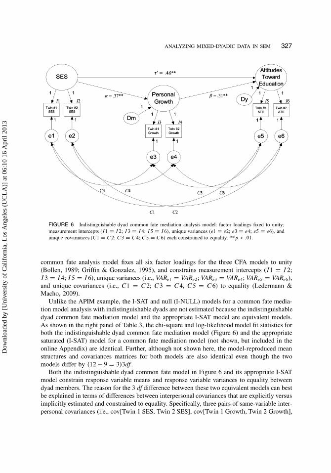
FIGURE 6 Indistinguishable dyad common fate mediation analysis model: factor loadings fixed to unity;

measurement intercepts (I1 D I2; I3 D I4; I5 D I6), unique variances (e1 D e2; e3 D e4; e5 D e6), and

unique covariances (C1 D C 2; C 3 D C 4; C 5 D C 6) each constrained to equality. **p < :01.

common fate analysis model fixes all six factor loadings for the three CFA models to unity

(Bollen, 1989; Griffin & Gonzalez, 1995), and constrains measurement intercepts (I1 D I2;

I3 D I4; I5 D I6), unique variances (i.e., VARe1 D VARe2; VARe3 D VARe4; VARe5 D VARe6),

and unique covariances (i.e., C1 D C2; C3 D C4, C5 D C6) to equality (Ledermann &

Macho, 2009).

Unlike the APIM example, the I-SAT and null (I-NULL) models for a common fate media-

tion model analysis with indistinguishable dyads are not estimated because the indistinguishable

dyad common fate mediation model and the appropriate I-SAT model are equivalent models.

As shown in the right panel of Table 3, the chi-square and log-likelihood model fit statistics for

both the indistinguishable dyad common fate mediation model (Figure 6) and the appropriate

saturated (I-SAT) model for a common fate mediation model (not shown, but included in the

online Appendix) are identical. Further, although not shown here, the model-reproduced mean

structures and covariances matrices for both models are also identical even though the two

models differ by .12 � 9 D 3/3df .

Both the indistinguishable dyad common fate model in Figure 6 and its appropriate I-SAT

model constrain response variable means and response variable variances to equality between

dyad members. The reason for the 3 df difference between these two equivalent models can best

be explained in terms of differences between interpersonal covariances that are explicitly versus

implicitly estimated and constrained to equality. Specifically, three pairs of same-variable inter-

personal covariances (i.e., cov[Twin 1 SES, Twin 2 SES], cov[Twin 1 Growth, Twin 2 Growth],

Dow

nloa

ded

by [

Uni

vers

ity o

f C

alif

orni

a, L

os A

ngel

es (

UC

LA

)] a

t 06:

10 1

6 A

pril

2013


cov[Twin 1 ATE Twin 2 ATE]) that would be freely estimated in the appropriate I-SAT model

are not included or estimated in the common fate model (i.e., cov[e1; e2], cov[e3; e4], and

cov[e5; e6], respectively, are not estimated in Figure 6). The common fate model addresses

this interpersonal dyadic dependence by estimating three shared latent variable variances rather

than three interpersonal covariances, as described earlier. The 3 df difference between the two

models comes from the remaining three interpersonal covariances (i.e., cov[Twin 1 SES, Twin 2

ATE] D cov[Twin 1 ATE, Twin 2 SES]; cov[Twin 1 SES, Twin 2 Growth] D cov[Twin 2 SES,

Twin 1 Growth; cov[Twin 1 Growth, Twin 2 ATE] D cov[Twin 2 Growth, Twin 1 ATE]) that

(a) would be explicitly estimated and constrained to equality (using 3 df) in the I-SAT model,

(b) are not explicitly included or estimated in Figure 6, but (c) are implicitly constrained to

equality (using 0 df) in the indistinguishable dyad common fate model-reproduced covariance

matrix as a direct result of the equality constraints (e1 D e2, e3 D e4, e5 D e6 and C1 D C2,

C3 D C4, C5 D C6) already included in the model.

As mentioned previously, if dyads were perfectly indistinguishable, the chi-square model fit

statistic would equal zero. The nonzero chi-square value shown in Table 3 (13.69) indicates

the SATSA twins are not perfectly indistinguishable. As also mentioned previously, saturated

models in general are not parsimonious and are seldom of interest to researchers. The in-

distinguishable dyad common fate mediation model is an example of a model that, although

essentially saturated in the indistinguishable dyad sense discussed previously, can still be used

to test a substantive research question involving mediation. However, similar to a model that is

saturated in the typical SEM sense, the question of fit for an indistinguishable dyad common

fate mediation model is a moot point; all fit indexes will show ideal values by definition.

Indistinguishable common fate example. To illustrate, the indistinguishable dyad com-

mon fate mediation model was used with the SATSA data to test whether a desire for personal

growth mediated the relationship between SES and attitudes toward education. As shown

in Figure 6, both regression path (’ & “) coefficients were statistically significant, which

suggested the possibility of mediation. The joint indirect path estimate .’“ D :12/ showed a

95% confidence interval (based on 5,000 bias-corrected bootstrap samples) that did not contain

zero [.05, .23]. A desire for personal growth partially mediated (as shown in Figure 6, the £0

path coefficient was also statistically significant) the relationship between SES and attitudes

toward education.

LONGITUDINAL DYADIC DATA ANALYSES

The actor–partner interdependence and common fate analysis models shown in the previous

sections can model dyadic data intrapersonal and interpersonal dependence and can quantify

dyadic relationship dynamics from data sampled cross-sectionally, but they cannot assess

dyadic response variable changes over time. However, the same intrapersonal and interpersonal

dyadic dependence can be modeled longitudinally to quantify separate, but related, changes

in dyad members’ response variable scores over time. An example of a latent growth curve

structural equation model (cf. Meredith & Tisak, 1990) that has been modified to accommodate

longitudinal dyadic data with covariates (e.g., DiLillo et al., 2009; Kashy, Donnellan, Burt, &

McGue, 2008) is shown in Figure 7. Recall that the Newlywed Project involved psychological

Dow

nloa

ded

by [

Uni

vers

ity o

f C

alif

orni

a, L

os A

ngel

es (

UC

LA

)] a

t 06:

10 1

6 A

pril

2013


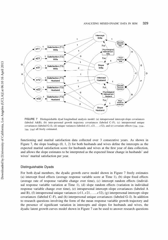
FIGURE 7 Distinguishable dyad longitudinal analysis model: (a) intrapersonal intercept-slope covariances

(labeled A&B), (b) inter-personal growth trajectory covariances (labeled C–F), (c) interpersonal unique

covariances (labeled G–I), (d) unique variances (labeled e11; e21; : : : e32), and (e) covariate effects (”IW, ”SW,

”IH, ”SH) all freely estimated.

functioning and marital satisfaction data collected over 3 consecutive years. As shown in

Figure 7, the slope loadings (0, 1, 2) for both husbands and wives define the intercepts as the

expected marital satisfaction score for husbands and wives at the first year of data collection,

and allows the slope estimates to be interpreted as the expected linear change in husbands’ and

wives’ marital satisfaction per year.

Distinguishable Dyads

For both dyad members, the dyadic growth curve model shown in Figure 7 freely estimates

(a) intercept fixed effects (average response variable score at Time 1), (b) slope fixed effects

(average rate of response variable change over time), (c) intercept random effects (individ-

ual response variable variation at Time 1), (d) slope random effects (variation in individual

response variable change over time), (e) intrapersonal intercept–slope covariances (labeled A

and B), (f) intrapersonal unique variances (e11; e21; : : : ; e32), (g) interpersonal intercept–slope

covariances (labeled C–F), and (h) interpersonal unique covariances (labeled G–I). In addition

to research questions involving the form of the mean response variable growth trajectory and

the presence of significant variation in intercepts and slopes for husbands and wives, the

dyadic latent growth curves model shown in Figure 7 can be used to answer research questions

Dow

nloa

ded

by [

Uni

vers

ity o

f C

alif

orni

a, L

os A

ngel

es (

UC

LA

)] a

t 06:

10 1

6 A

pril

2013


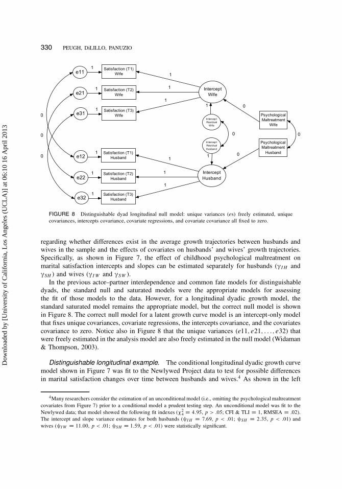
FIGURE 8 Distinguishable dyad longitudinal null model: unique variances (es) freely estimated, unique

covariances, intercepts covariance, covariate regressions, and covariate covariance all fixed to zero.

regarding whether differences exist in the average growth trajectories between husbands and

wives in the sample and the effects of covariates on husbands’ and wives’ growth trajectories.

Specifically, as shown in Figure 7, the effect of childhood psychological maltreatment on

marital satisfaction intercepts and slopes can be estimated separately for husbands (”IH and

”SH ) and wives (”I W and ”SW ).

In the previous actor–partner interdependence and common fate models for distinguishable

dyads, the standard null and saturated models were the appropriate models for assessing

the fit of those models to the data. However, for a longitudinal dyadic growth model, the

standard saturated model remains the appropriate model, but the correct null model is shown

in Figure 8. The correct null model for a latent growth curve model is an intercept-only model

that fixes unique covariances, covariate regressions, the intercepts covariance, and the covariates

covariance to zero. Notice also in Figure 8 that the unique variances (e11; e21; : : : ; e32) that

were freely estimated in the analysis model are also freely estimated in the null model (Widaman

& Thompson, 2003).

Distinguishable longitudinal example. The conditional longitudinal dyadic growth curve

model shown in Figure 7 was fit to the Newlywed Project data to test for possible differences

in marital satisfaction changes over time between husbands and wives.4 As shown in the left

4Many researchers consider the estimation of an unconditional model (i.e., omitting the psychological maltreatment

covariates from Figure 7) prior to a conditional model a prudent testing step. An unconditional model was fit to the

Newlywed data; that model showed the following fit indexes (¦24 D 4:95, p > :05; CFI & TLI D 1, RMSEA D .02).

The intercept and slope variance estimates for both husbands (§IH D 7:69, p < :01; §SH D 2:35, p < :01) and

wives (§IW D 11:00, p < :01; §SH D 1:59, p < :01) were statistically significant.

Dow

nloa

ded

by [

Uni

vers

ity o

f C

alif

orni

a, L

os A

ngel

es (

UC

LA

)] a

t 06:

10 1

6 A

pril

2013


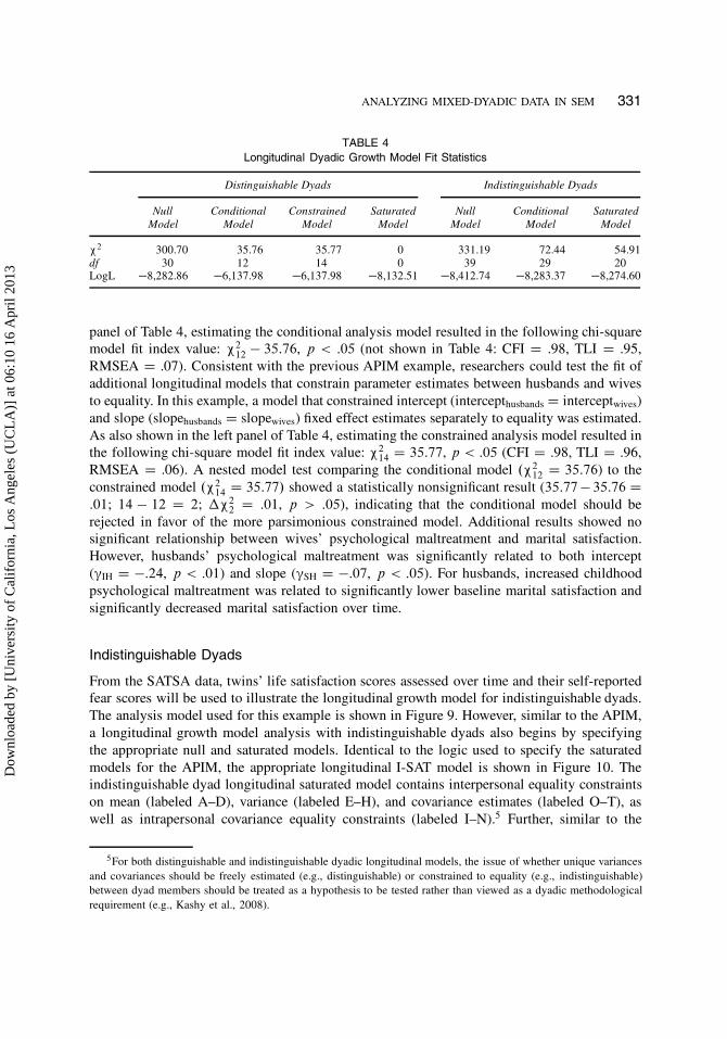
TABLE 4

Longitudinal Dyadic Growth Model Fit Statistics


Null

Model

Conditional

Model

Constrained

Model

Saturated

Model

Null

Model

Conditional

Model

Saturated

Model

¦2 300.70 35.76 35.77 0 331.19 72.44 54.91

df 30 12 14 0 39 29 20LogL �8,282.86 �6,137.98 �6,137.98 �8,132.51 �8,412.74 �8,283.37 �8,274.60

panel of Table 4, estimating the conditional analysis model resulted in the following chi-square

model fit index value: ¦212

� 35:76, p < :05 (not shown in Table 4: CFI D .98, TLI D .95,

RMSEA D .07). Consistent with the previous APIM example, researchers could test the fit of

additional longitudinal models that constrain parameter estimates between husbands and wives

to equality. In this example, a model that constrained intercept (intercepthusbands D interceptwives)

and slope (slopehusbands D slopewives) fixed effect estimates separately to equality was estimated.

As also shown in the left panel of Table 4, estimating the constrained analysis model resulted in

the following chi-square model fit index value: ¦214 D 35:77, p < :05 (CFI D .98, TLI D .96,

RMSEA D .06). A nested model test comparing the conditional model .¦212 D 35:76) to the

constrained model .¦214 D 35:77/ showed a statistically nonsignificant result (35:77 � 35:76 D

:01; 14 � 12 D 2; �¦22 D :01, p > :05), indicating that the conditional model should be

rejected in favor of the more parsimonious constrained model. Additional results showed no

significant relationship between wives’ psychological maltreatment and marital satisfaction.

However, husbands’ psychological maltreatment was significantly related to both intercept

(”IH D �:24, p < :01) and slope (”SH D �:07, p < :05). For husbands, increased childhood

psychological maltreatment was related to significantly lower baseline marital satisfaction and

significantly decreased marital satisfaction over time.

Indistinguishable Dyads

From the SATSA data, twins’ life satisfaction scores assessed over time and their self-reported

fear scores will be used to illustrate the longitudinal growth model for indistinguishable dyads.

The analysis model used for this example is shown in Figure 9. However, similar to the APIM,

a longitudinal growth model analysis with indistinguishable dyads also begins by specifying

the appropriate null and saturated models. Identical to the logic used to specify the saturated

models for the APIM, the appropriate longitudinal I-SAT model is shown in Figure 10. The

indistinguishable dyad longitudinal saturated model contains interpersonal equality constraints

on mean (labeled A–D), variance (labeled E–H), and covariance estimates (labeled O–T), as

well as intrapersonal covariance equality constraints (labeled I–N).5 Further, similar to the

5For both distinguishable and indistinguishable dyadic longitudinal models, the issue of whether unique variances

and covariances should be freely estimated (e.g., distinguishable) or constrained to equality (e.g., indistinguishable)

between dyad members should be treated as a hypothesis to be tested rather than viewed as a dyadic methodological

requirement (e.g., Kashy et al., 2008).

Dow

nloa

ded

by [

Uni

vers

ity o

f C

alif

orni

a, L

os A

ngel

es (

UC

LA

)] a

t 06:

10 1

6 A

pril

2013


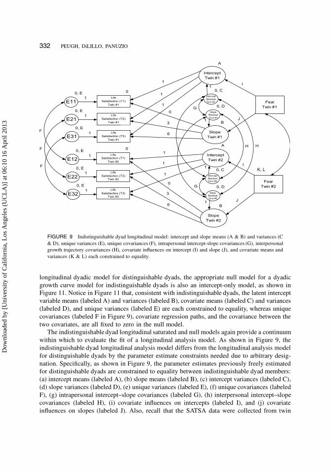
FIGURE 9 Indistinguishable dyad longitudinal model: intercept and slope means (A & B) and variances (C

& D), unique variances (E), unique covariances (F), intrapersonal intercept-slope covariances (G), interpersonal

growth trajectory covariances (H), covariate influences on intercept (I) and slope (J), and covariate means and

variances (K & L) each constrained to equality.

longitudinal dyadic model for distinguishable dyads, the appropriate null model for a dyadic

growth curve model for indistinguishable dyads is also an intercept-only model, as shown in

Figure 11. Notice in Figure 11 that, consistent with indistinguishable dyads, the latent intercept

variable means (labeled A) and variances (labeled B), covariate means (labeled C) and variances

(labeled D), and unique variances (labeled E) are each constrained to equality, whereas unique

covariances (labeled F in Figure 9), covariate regression paths, and the covariance between the

two covariates, are all fixed to zero in the null model.

The indistinguishable dyad longitudinal saturated and null models again provide a continuum

within which to evaluate the fit of a longitudinal analysis model. As shown in Figure 9, the

indistinguishable dyad longitudinal analysis model differs from the longitudinal analysis model

for distinguishable dyads by the parameter estimate constraints needed due to arbitrary desig-

nation. Specifically, as shown in Figure 9, the parameter estimates previously freely estimated

for distinguishable dyads are constrained to equality between indistinguishable dyad members:

(a) intercept means (labeled A), (b) slope means (labeled B), (c) intercept variances (labeled C),

(d) slope variances (labeled D), (e) unique variances (labeled E), (f) unique covariances (labeled

F), (g) intrapersonal intercept–slope covariances (labeled G), (h) interpersonal intercept–slope

covariances (labeled H), (i) covariate influences on intercepts (labeled I), and (j) covariate

influences on slopes (labeled J). Also, recall that the SATSA data were collected from twin

Dow

nloa

ded

by [

Uni

vers

ity o

f C

alif

orni

a, L

os A

ngel

es (

UC

LA

)] a

t 06:

10 1

6 A

pril

2013


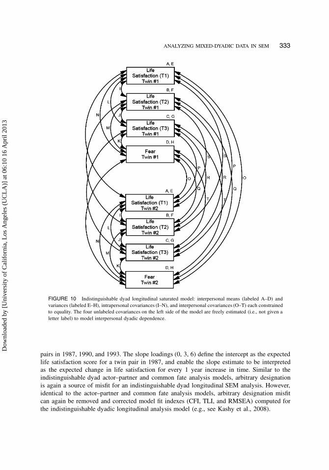
FIGURE 10 Indistinguishable dyad longitudinal saturated model: interpersonal means (labeled A–D) and

variances (labeled E–H), intrapersonal covariances (I–N), and interpersonal covariances (O–T) each constrained

to equality. The four unlabeled covariances on the left side of the model are freely estimated (i.e., not given a

letter label) to model interpersonal dyadic dependence.

pairs in 1987, 1990, and 1993. The slope loadings (0, 3, 6) define the intercept as the expected

life satisfaction score for a twin pair in 1987, and enable the slope estimate to be interpreted

as the expected change in life satisfaction for every 1 year increase in time. Similar to the

indistinguishable dyad actor–partner and common fate analysis models, arbitrary designation

is again a source of misfit for an indistinguishable dyad longitudinal SEM analysis. However,

identical to the actor–partner and common fate analysis models, arbitrary designation misfit

can again be removed and corrected model fit indexes (CFI, TLI, and RMSEA) computed for

the indistinguishable dyadic longitudinal analysis model (e.g., see Kashy et al., 2008).

Dow

nloa

ded

by [

Uni

vers

ity o

f C

alif

orni

a, L

os A

ngel

es (

UC

LA

)] a

t 06:

10 1

6 A

pril

2013


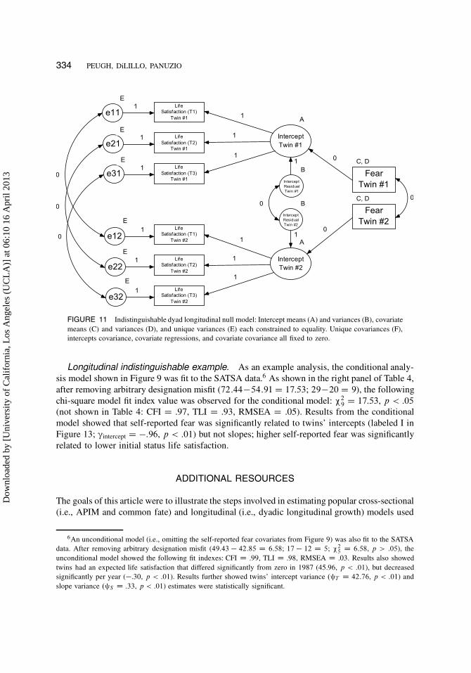
FIGURE 11 Indistinguishable dyad longitudinal null model: Intercept means (A) and variances (B), covariate

means (C) and variances (D), and unique variances (E) each constrained to equality. Unique covariances (F),

intercepts covariance, covariate regressions, and covariate covariance all fixed to zero.

Longitudinal indistinguishable example. As an example analysis, the conditional analy-

sis model shown in Figure 9 was fit to the SATSA data.6 As shown in the right panel of Table 4,

after removing arbitrary designation misfit (72:44�54:91 D 17:53; 29�20 D 9), the following

chi-square model fit index value was observed for the conditional model: ¦29 D 17:53, p < :05

(not shown in Table 4: CFI D .97, TLI D .93, RMSEA D .05). Results from the conditional

model showed that self-reported fear was significantly related to twins’ intercepts (labeled I in

Figure 13; ”intercept D �:96, p < :01) but not slopes; higher self-reported fear was significantly

related to lower initial status life satisfaction.

ADDITIONAL RESOURCES

The goals of this article were to illustrate the steps involved in estimating popular cross-sectional

(i.e., APIM and common fate) and longitudinal (i.e., dyadic longitudinal growth) models used

6An unconditional model (i.e., omitting the self-reported fear covariates from Figure 9) was also fit to the SATSA

data. After removing arbitrary designation misfit (49:43 � 42:85 D 6:58; 17 � 12 D 5; ¦25 D 6:58, p > :05), the

unconditional model showed the following fit indexes: CFI D .99, TLI D .98, RMSEA D .03. Results also showed

twins had an expected life satisfaction that differed significantly from zero in 1987 (45.96, p < :01), but decreased

significantly per year (�.30, p < :01). Results further showed twins’ intercept variance .§T D 42:76, p < :01) and

slope variance .§S D :33, p < :01) estimates were statistically significant.

Dow

nloa

ded

by [

Uni

vers

ity o

f C

alif

orni

a, L

os A

ngel

es (

UC

LA

)] a

t 06:

10 1

6 A

pril

2013


to analyze mixed-dyadic data collected from indistinguishable or distinguishable dyads, and

to clarify why certain additional steps and modifications are needed to analyze indistinguish-

able dyad data using structural equation models. The AMOS and Mplus statistical analysis

software packages were used in all analysis models presented in this article; all examples are

available in an appendix online at https://bmixythos.cchmc.org/xythoswfs/webui/_xy-476611_

1-t_AXKarXYG. However, a secondary goal of this article was to provide sufficient detail to

allow researchers to analyze these models in the analysis software package of their choice.

In addition to the models illustrated here, several authors have proposed additional cross-

sectional and longitudinal dyadic data analysis models. For example, Newsom (2002) showed

how a CFA model could also be used to test for significant differences among distinguishable

dyad members. Also, Laurenceau and Bolger (2005) showed how diary methods can be used to

quantify relationship process changes over time in marital data. Further, although most dyadic

data analysis models assume a response variable measured on a continuous scale, each of these

models can be used to analyze cross-sectional and longitudinal response variables measured on

a categorical scale (e.g., see Kenny et al., 2006). In addition, many of the SEM models shown

here and elsewhere can also be equivalently estimated as hierarchical linear models (e.g., see

Atkins, 2005; Campbell & Kashy, 2002; Gonzalez & Griffin, 2002; Kashy, Campbell, & Harris,

2006; Wendorf, 2002; Whisman, Uebelacker, & Weinstock, 2004; Zhang & Willson, 2006).

The dyadic models demonstrated in this article have also been combined and expanded on

in several ways. Kenny and Ledermann (2010) showed how the APIM can be modified so that

the individual-level actor and partner effects can be used to identify dyad-level relationship

patterns (e.g., actor only, partner only, couple, and contrast patterns). Several researchers have

also shown how the APIM can be expanded to address dyadic research questions involving mod-

erated mediation and mediated moderation possibilities (e.g., Bodenmann, Ledermann, & Brad-

bury, 2007; Campbell, Simpson, Kashy, & Fletcher, 2001; Ledermann & Bodenmann, 2006;

Srivastava, McGonigal, Richards, Butler, & Gross, 2006). In addition, Matthews, Conger, and

Wickrama (1996) showed how the common fate and actor partner interdependence models can

be combined, and more than one mediating variable added, to answer complex dyadic research

questions involving how mediated dynamics at the individual level can impact the relationship

at the dyad level. Needless to say, applied researchers seeking to answer research questions

involving cross-sectional or longitudinal mixed dyadic data collected from dyads considered to

be distinguishable or indistinguishable can choose from among several SEM analysis options.

ACKNOWLEDGMENTS

We wish to extend our appreciation and gratitude to Craig K. Enders, Joseph A. Olsen, Pamela

Sadler, Erik Woody, the Teacher’s Corner Editor, and several anonymous reviewers for their

insightful comments and helpful suggestions that greatly improved the quality of this article.

REFERENCES

Atkins, D. C. (2005). Using multilevel models to analyze couple and family treatment data: Basic and advanced issues.

Journal of Family Psychology, 19, 98–110.

Dow

nloa

ded

by [

Uni

vers

ity o

f C

alif

orni

a, L

os A

ngel

es (

UC

LA

)] a

t 06:

10 1

6 A

pril

2013


Bodenmann, G., Ledermann, T., & Bradbury, T. N. (2007). Stress, sex, and satisfaction in marriage. Personal Relation-

ships, 14, 551–569.

Bollen, K. A. (1989). Structural equations with latent variables. New York, NY: Wiley.

Campbell, L., & Kashy, D. A. (2002). Estimating actor, partner, and interaction effects for dyadic data using PROC

MIXED and HLM: A user-friendly guide. Personal Relationships, 9, 327–342.

Campbell, L., Simpson, J. A., Kashy, D. A., & Fletcher, G. J. O. (2001). Ideal standards, the self, and flexibility of

ideals in close relationships. Personality and Social Psychology Bulletin, 27, 447–462.

Carey, G. (2005). The intraclass covariance matrix. Behavior Genetics, 35, 667–670.

Cook, W. L., & Kenny, D. A. (2005). The actor–partner interdependence model: A model of bidirectional effects in

developmental studies. International Journal of Behavioral Development, 29, 101–109.

DiLillo, D., Peugh, J., Walsh, K., Panuzio, J., Trask, E., & Evans, S. (2009). Child maltreatment history among

newlywed couples: A longitudinal study of marital outcomes and mediating pathways. Journal of Consulting and

Clinical Psychology, 77, 680–692.

Efron, B., & Tibshirani, R. J. (1993). An introduction to the bootstrap. New York, NY: Chapman & Hall/CRC.

Fritz, M. S., & MacKinnon, D. P. (2007). Required sample size to detect the mediated effect. Psychological Science,

18, 233–239.

Furman, W., & Simon, V. A. (2006). Actor and partner effects of adolescents’ romantic working models and styles of

interactions with romantic partners. Child Development, 77, 588–604.

Gonzalez, R., & Griffin, D. (1999). The correlational analysis of dyad-level data in the distinguishable case. Personal

Relationships, 6, 449–469.

Gonzalez, R., & Griffin, D. (2001). Testing parameters in structural equation modeling: Every “one” matters. Psycho-

logical Methods, 6, 258–269.

Gonzalez, R., & Griffin, D. (2002). Modeling the personality of dyads and groups. Journal of Personality, 70, 901–924.

Griffin, D., & Gonzalez, R. (1995). Correlational analysis of dyad-level data in the exchangeable case. Psychological

Bulletin, 118, 430–439.

Kashy, D. A., Campbell, L., & Harris, D. W. (2006). Advances in data analytic approaches for relationships research:

The broad utility of hierarchical linear modeling. In A. Vangelisti & D. Perlman (Eds.), Cambridge handbook of

personal relationships (pp. 73–89). New York, NY: Cambridge University Press.

Kashy, D. A., Donnellan, M. B., Burt, S. A., & McGue, M. (2008). Growth curve models for indistinguishable

dyads using multilevel modeling and structural equation modeling: The case of adolescent twins’ conflict with their

mothers. Developmental Psychology, 44, 316–329.

Kenny, D. A. (1996). Models of non-independence in dyadic research. Journal of Social and Personal Relationships,

13, 279–294.

Kenny, D. A., & Cook, W. (1999). Partner effects in relationship research: Conceptual issues, analytic difficulties, and

illustrations. Personal Relationships, 6, 433–448.

Kenny, D. A., & Judd, C. M. (1996). A general procedure for the estimation of interdependence. Psychological Bulletin,

119, 138–148.

Kenny, D. A., Kashy, D. A., & Bolger, N. (1998). Data analysis in social psychology. In D. T. Gilbert, S. T. Fiske, &

G. Lindzey (Eds.), Handbook of social psychology (4th ed., Vol. 1, pp. 233–265). Boston, MA: McGraw-Hill.

Kenny, D. A., Kashy, D. A., & Cook, W. L. (2006). Dyadic data analysis. New York, NY: Guilford.

Kenny, D. A., & LaVoie, L. (1985). Separating individual and group effects. Journal of Personality and Social

Psychology, 48, 339–348.

Kenny, D. A., & Ledermann, T. (2010). Detecting, measuring, and testing dyadic patterns in the actor–partner inter-

dependence model. Journal of Family Psychology, 24, 359–366.

Laurenceau, J. P., & Bolger, N. (2005). Using diary methods to study marital and family processes. Journal of Family

Psychology, 19, 86–97.

Ledermann, T., & Bodenmann, G. (2006). Moderator- und mediator-effekte bei dyadischen daten: Zwei erweiterungen

des akteurpartner-interdependenz-modells [Moderator and mediator effects in dyadic research: Two extensions of

the actor–partner interdependence model]. Zeitschrift für Sozialpsychologie, 37, 27–40.

Ledermann, T., & Macho, S. (2009). Mediation in dyadic data at the level of the dyads: A structural equation modeling

approach. Journal of Family Psychology, 23, 661–670.

MacKinnon, D. P. (2008). Introduction to statistical mediation analysis. New York, NY: Erlbaum.

MacKinnon, D. P., Lockwood, C. M., Hoffman, J. M., West, S. G., & Sheets, V. (2002). A comparison of methods to

test mediation and other intervening variable effects. Psychological Methods, 7, 83–104.

Dow

nloa

ded

by [

Uni

vers

ity o

f C

alif

orni

a, L

os A

ngel

es (

UC

LA

)] a

t 06:

10 1

6 A

pril

2013


MacKinnon, D. P., Lockwood, C. M., & Williams, J. (2004). Confidence limits for the indirect effect: Distribution of

the product and resampling methods. Multivariate Behavioral Research, 39, 99–128.

Matthews, L. S., Conger, R. D., & Wickrama, K. A. S. (1996). Work–family conflict and marital quality: Mediating

processes. Social Psychology Quarterly, 59, 62–79.

McGraw, K. O., & Wong, S. P. (1996). Forming inferences about some intraclass correlation coefficients. Psychological

Methods, 1, 30–46.

Meredith, W., & Tisak, J. (1990). Latent curve analysis. Psychometrika, 55, 107–122.

Muthén, B. O., & Muthén, L. K. (1998–2010). Mplus user’s guide (6th ed.). Los Angeles, CA: Muthén & Muthén.

Newsom, J. T. (2002). A multilevel structural equation model for dyadic data. Structural Equation Modeling, 9,

431–447.

Olsen, J. A., & Kenny, D. A. (2006). Structural equation modeling with interchangeable dyads. Psychological Methods,

11, 127–141.

Pedersen, N. L. (2004). Swedish Adoption/Twin Study on Aging (SATSA), 1984, 1987, 1990, and 1993 [Computer file].

ICPSR version. Stockholm, Sweden: Karolinska Institutet [producer]. Ann Arbor, MI: Inter-University Consortium

for Political and Social Research [distributor].

Srivastava, S., McGonigal, K. M., Richards, J. M., Butler, E. A., & Gross, J. J. (2006). Optimism in close relationships:

How seeing things in a positive light makes them so. Journal of Personality and Social Psychology, 91, 143–153.

Wendorf, C. A. (2002). Comparisons of structural equation modeling and hierarchical linear modeling approaches to

couples’ data. Structural Equation Modeling, 9, 126–140.

Whisman, M. A., Uebelacker, L. A., & Weinstock, L. M. (2004). Psychopathology and marital satisfaction: The

importance of evaluating both partners. Journal of Consulting and Clinical Psychology, 72, 830–838.

Widaman, K. F., & Thompson, J. S. (2003). On specifying the null model for incremental fit indices in structural

equation modeling. Psychological Methods, 8, 16–37.

Woody, E., & Sadler, P. (2005). Structural equation models for interchangeable dyads: Being the same makes a dif-

ference. Psychological Methods, 10, 139–158.

Zhang, D., & Willson, V. L. (2006). Comparing empirical power of multilevel structural equation models and

hierarchical linear models: Understanding cross-level interactions. Structural Equation Modeling, 13, 615–630.

Dow

nloa

ded

by [

Uni

vers

ity o

f C

alif

orni

a, L

os A

ngel

es (

UC

LA

)] a

t 06:

10 1

6 A

pril

2013

Documents

Analyzing Mixed-Dyadic Data Using Structural Equation … · (e.g., Kenny & Ledermann, 2010). For example, individuals making up a traditional marital