lable at ScienceDirect

Environmental Modelling & Software 94 (2017) 127e139

Contents lists avai

Environmental Modelling & Software

journal homepage: www.elsevier .com/locate/envsoft

Application of the space-for-time substitution method in validatinglong-term biomass predictions of a forest landscape model

Jun Ma a, Xiangming Xiao a, b, *, Rencang Bu c, Russell Doughty b, Yuanman Hu c,Bangqian Chen a, d, Xiangping Li a, Bin Zhao a

a Ministry of Education Key Laboratory for Biodiversity Science and Ecological Engineering, Institute of Biodiversity Science, Fudan University, Shanghai,200433, PR Chinab Department of Microbiology and Plant Biology, Center for Spatial Analysis, University of Oklahoma, Norman, OK 73019, USAc Institute of Applied Ecology, Chinese Academy of Sciences, Shenyang, 110016, PR Chinad Danzhou Investigation & Experiment Station of Tropical Cops, Ministry of Agriculture, Rubber Research Institute, Chinese Academy of Tropical AgriculturalSciences (CATAS), Danzhou 571737, PR China

a r t i c l e i n f o

Article history:Received 29 April 2016Received in revised form6 April 2017Accepted 14 April 2017

Keywords:Forest landscape modelsLANDIS-II modelForest biomassForest ageSpace-for-timeNortheastern China

* Corresponding author.E-mail address: xiangming.xiao@ou.edu (X. Xiao).

http://dx.doi.org/10.1016/j.envsoft.2017.04.0041364-8152/© 2017 Elsevier Ltd. All rights reserved.

a b s t r a c t

Validation of the long-term biomass predictions of forest landscape models (FLMs) has always been achallenging task. Using the space-for-time substitution method, forest biomass curves over stand agewere generated from a forest survey dataset (FSD) in the Lesser Khingan Mountains area (LKM),Northeastern China and compared with long-term biomass predictions of LANDIS-II model. The resultsshowed that mean forest age and mean biomass of the LKM in 2000 were 51.6 years and 84.2 Mg ha�1,respectively. Significant linear correlations were found between FSD derived biomass and simulatedbiomass in the aggradation phase for the entire LKM and most subregions. However, a considerabledifference in the mean maximum biomass (53.45 Mg ha�1) existed between from FSD and simulationduring the post-aggradation phase. The space-for-time substitution method has potential in validatingtime series biomass predictions of FLMs in aggradation phase when only limited forest inventory data isavailable.

© 2017 Elsevier Ltd. All rights reserved.

1. Introduction

Forests are a key component of terrestrial ecosystems and playan important role in the global carbon cycle (Birdsey et al., 2006;Dixon et al., 1994; Houghton and Hackler, 2000). Predictions offorest biomass and its spatial distribution are essential for evalu-ating how forests contribute to climate change mitigation (Keithet al., 2009; Saatchi et al., 2011). Forest landscape models (FLMs)are generally used to simulate forest biomass, species composition,and stand structure at large spatiotemporal extents (Gustafsonet al., 2010; He et al., 1999; Scheller et al., 2007; Scheller andMladenoff, 2004). The effects of forest management (Schelleret al., 2011a, 2011b), climate change (He et al., 2005; Ma et al.,2014b), and disturbances (He and Mladenoff, 1999) on forest suc-cession dynamics, such as biomass accumulation and species dis-tribution, can also be explored in FLMs. However, the credibility of

predictions, especially forest biomass, directly determines thescope and applicability of FLMs in forest management (Gardner andUrban, 2003; Shifley et al., 2009; Tian et al., 2016; Wang et al.,2014b). Thus, it is important to evaluate FLMs predictions withobservational data.

Traditionally, the evaluation of simulated results of most FLMs isconducted by comparing the predictions with results from empir-ical knowledge, other model outputs, and/or field observation data(Blanco et al., 2007; Busing et al., 2007; Ma et al., 2014a). Forexample, field collected datawere used to validate the phenologicalpredictions of the PHENIPS model in Bohemian forests (Berec et al.,2013). The productivity and cycling of carbon and nitrogen in aspenforests were simulated in five differentmodels, and the results frommultiple models were cross validated (Wang et al., 2014a). Monthlycarbon flux data were used to calibrate and validate the results ofthe LANDIS-II model, which was used to simulate forest carbonsequestration under different fire regimes (Scheller et al., 2011b). ATROLL simulation of tropical rainforest spatial patterns wascompared to field sampling data to validate predicted forest suc-cession processes (Chave,1999). However, most validations of FLMs

Model description

Model name LANDIS-IIDevelopers Eric Gustafson, USDA Forest Service; David

Mladenoff, University of Wisconsin-Madison;Robert Scheller, Portland State University; BrainStuturvant, USDA Forest Service; JonathanThompson, Harvard Forest

Contact Information Dr. Robert Scheller, Department ofEnvironmental Sciences andManagement, Portland State University.Email: rmschell@pdx.edu

Year First Available 2004Hardware Required No special requirementsSoftware Required Windows, Mac OSX, or LinuxAvailability Free (downloading site: http://www.landis-ii.

org/install)Program Language C#Data Form of Repository Files and Spreadsheet

J. Ma et al. / Environmental Modelling & Software 94 (2017) 127e139128

predictions were conducted at a specific site and time, which do notmatch the large spatiotemporal extents used in FLM simulations.

One of the ideal methods to improve the short-term predictionsof FLMs is to conduct model calibration by comparing model pre-dictions with time-series in-situ field data at appropriate spatio-temporal scales (Schmitz, 1997; Tsoar et al., 2007; Zaniewski et al.,2002). The model calibration has been proved to improve thecredibility of predictions in ecological models based on a largeamount of ecological data (Marcot et al., 2006; Wang et al., 2014b).Forest inventory data has been adopted by forest modeling studiesto calibrate and validate predictions made by ecological models,which has enhanced the performance of the models (Peng et al.,2011). FLMs are parameterized using complex field-collected dataat landscape scale, and the validation of FLM results, generally re-quires a multitude of long-term observation data. However, thiskind of data is not available for most forest areas in the world.Chronological forest inventory data can be used effectively toimprove the predictions of FLMs. For example, LANDIS Pro is adynamic FLM that simulates processes like forest succession, seeddispersal, species establishment, and disturbances (Gustafson et al.,2000; He et al., 1999; Ma et al., 2014b). Biomass can also besimulated in this model by tracking tree species cohorts and theiramounts of the landscape. A recent study proposed a framework forevaluating short-term predictions of the LANDIS Pro model basedon a series of historical forest inventory data (Wang et al., 2014b).

Ground-based forest survey data, such as the U.S. Forest In-ventory and Analysis (FIA) data, are increasingly abundant andeasily obtained. However, similar data that are appropriate forcomparison with the long-term predictions of FLMs are still scarcefor forests in China. Theoretical and empirical knowledge are usu-ally used to judge the long-term predictions and adjust the initialparameters of FLMs of forest regions in Northeastern China (He,2008). Generally, different forest succession stages were regardedas representative moments of forest growing process, and mea-surements of their biomass have been used to predict the trajec-tories of forest carbon sequestration (Larsen et al., 2010; Ma et al.,2015; Wang et al., 2014b). However, great uncertainties exist inforest biomass accumulation over time when considering onlyspecific states of succession. Also, climate change and disturbanceinfluences forest biomass accumulation processes to a considerableextent (Chiang et al., 2008; Li et al., 2000; McMahon et al., 2010; Xu

et al., 2012). Therefore, time series forest biomass survey data isessential for calibrating long-term FLM simulations, however, thisdata is difficult to acquire. Fortunately, based on the space-for-timesubstitution method, observed forest biomass at different standages can be used to compare with the long-term biomass pre-dictions of FLMs.

Forest survey dataset (FSD) is generated based on differentforest management units in China at regular intervals (every 10years) and contain abundant information such as species compo-sition, tree ages, and timber volume (Dong et al., 2008). From FSD,we can obtain information on the spatial distribution of vegetationcommunities, stand ages, and biomass. This dataset is commonlyused to parameterize FLMs such as LANDIS Pro and LANDIS-II (Buet al., 2008a; He et al., 2005). The space-for-time substitutionmethod can be adopted to validate long-term forest biomass sim-ulations by assuming that the biomass of old-growth forest is thefuture state of the younger forests. Therefore, this methodmight beuseful for validating long-term biomass predictions of FLMs,especially when only limited forest inventory data is available.

In this study, the LANDIS-II model was used to illustrate how thespace-for-time substitution method is applied to validate long-term biomass predictions based on FSD derived forest age andbiomass data. FSD of 2000 was used to calculate forest biomassdynamicswith different stand ages in different regions in the LesserKhingan Mountains area (LKM) of Northeastern China, and theforest biomass-age curves were compared with simulated biomassof LANDIS-II model for the entire LKM and its subregions. The ob-jectives of this studywere to (1) generate forest biomass-age curvesbased on the FSD of the LKM in the year 2000; (2) simulate biomassdynamics from 2000 to 2300 using LANDIS-II model; and (3)explore the performance of the space-for-time substitutionmethodin the validation of biomass predictions by the LANDIS-II model.

2. Materials and methods

2.1. Study area

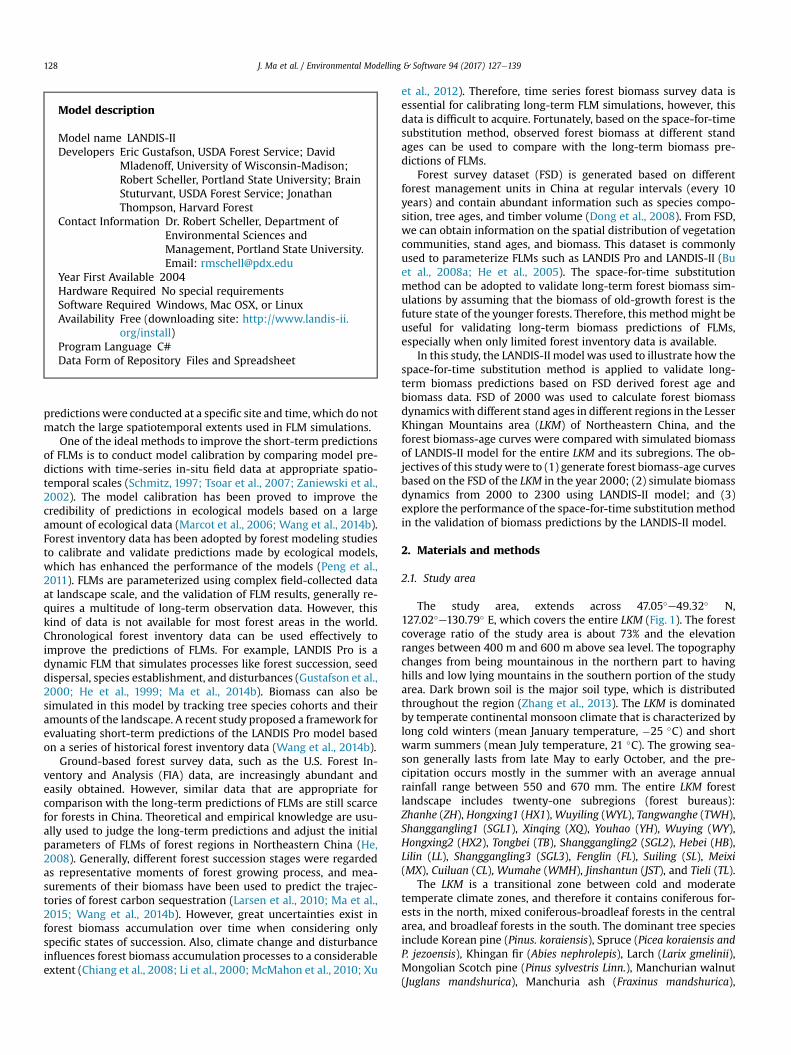
The study area, extends across 47.05�e49.32� N,127.02�e130.79� E, which covers the entire LKM (Fig. 1). The forestcoverage ratio of the study area is about 73% and the elevationranges between 400 m and 600 m above sea level. The topographychanges from being mountainous in the northern part to havinghills and low lying mountains in the southern portion of the studyarea. Dark brown soil is the major soil type, which is distributedthroughout the region (Zhang et al., 2013). The LKM is dominatedby temperate continental monsoon climate that is characterized bylong cold winters (mean January temperature, �25 �C) and shortwarm summers (mean July temperature, 21 �C). The growing sea-son generally lasts from late May to early October, and the pre-cipitation occurs mostly in the summer with an average annualrainfall range between 550 and 670 mm. The entire LKM forestlandscape includes twenty-one subregions (forest bureaus):Zhanhe (ZH), Hongxing1 (HX1),Wuyiling (WYL), Tangwanghe (TWH),Shanggangling1 (SGL1), Xinqing (XQ), Youhao (YH), Wuying (WY),Hongxing2 (HX2), Tongbei (TB), Shanggangling2 (SGL2), Hebei (HB),Lilin (LL), Shanggangling3 (SGL3), Fenglin (FL), Suiling (SL), Meixi(MX), Cuiluan (CL), Wumahe (WMH), Jinshantun (JST), and Tieli (TL).

The LKM is a transitional zone between cold and moderatetemperate climate zones, and therefore it contains coniferous for-ests in the north, mixed coniferous-broadleaf forests in the centralarea, and broadleaf forests in the south. The dominant tree speciesinclude Korean pine (Pinus. koraiensis), Spruce (Picea koraiensis andP. jezoensis), Khingan fir (Abies nephrolepis), Larch (Larix gmelinii),Mongolian Scotch pine (Pinus sylvestris Linn.), Manchurian walnut(Juglans mandshurica), Manchuria ash (Fraxinus mandshurica),

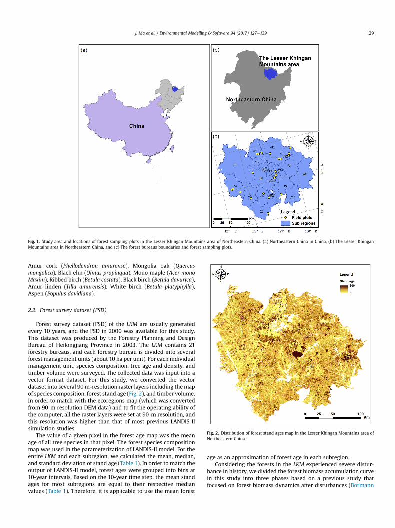
Fig. 1. Study area and locations of forest sampling plots in the Lesser Khingan Mountains area of Northeastern China. (a) Northeastern China in China, (b) The Lesser KhinganMountains area in Northeastern China, and (c) The forest bureaus boundaries and forest sampling plots.

J. Ma et al. / Environmental Modelling & Software 94 (2017) 127e139 129

Amur cork (Phellodendron amurense), Mongolia oak (Quercusmongolica), Black elm (Ulmus propinqua), Mono maple (Acer monoMaxim), Ribbed birch (Betula costata), Black birch (Betula davurica),Amur linden (Tilla amurensis), White birch (Betula platyphylla),Aspen (Populus davidiana).

Fig. 2. Distribution of forest stand ages map in the Lesser Khingan Mountains area ofNortheastern China.

2.2. Forest survey dataset (FSD)

Forest survey dataset (FSD) of the LKM are usually generatedevery 10 years, and the FSD in 2000 was available for this study.This dataset was produced by the Forestry Planning and DesignBureau of Heilongjiang Province in 2003. The LKM contains 21forestry bureaus, and each forestry bureau is divided into severalforest management units (about 10 ha per unit). For each individualmanagement unit, species composition, tree age and density, andtimber volume were surveyed. The collected data was input into avector format dataset. For this study, we converted the vectordataset into several 90m-resolution raster layers including themapof species composition, forest stand age (Fig. 2), and timber volume.In order to match with the ecoregions map (which was convertedfrom 90-m resolution DEM data) and to fit the operating ability ofthe computer, all the raster layers were set at 90-m resolution, andthis resolution was higher than that of most previous LANDIS-IIsimulation studies.

The value of a given pixel in the forest age map was the meanage of all tree species in that pixel. The forest species compositionmap was used in the parameterization of LANDIS-II model. For theentire LKM and each subregion, we calculated the mean, median,and standard deviation of stand age (Table 1). In order to match theoutput of LANDIS-II model, forest ages were grouped into bins at10-year intervals. Based on the 10-year time step, the mean standages for most subregions are equal to their respective medianvalues (Table 1). Therefore, it is applicable to use the mean forest

age as an approximation of forest age in each subregion.Considering the forests in the LKM experienced severe distur-

bance in history, we divided the forest biomass accumulation curvein this study into three phases based on a previous study thatfocused on forest biomass dynamics after disturbances (Bormann

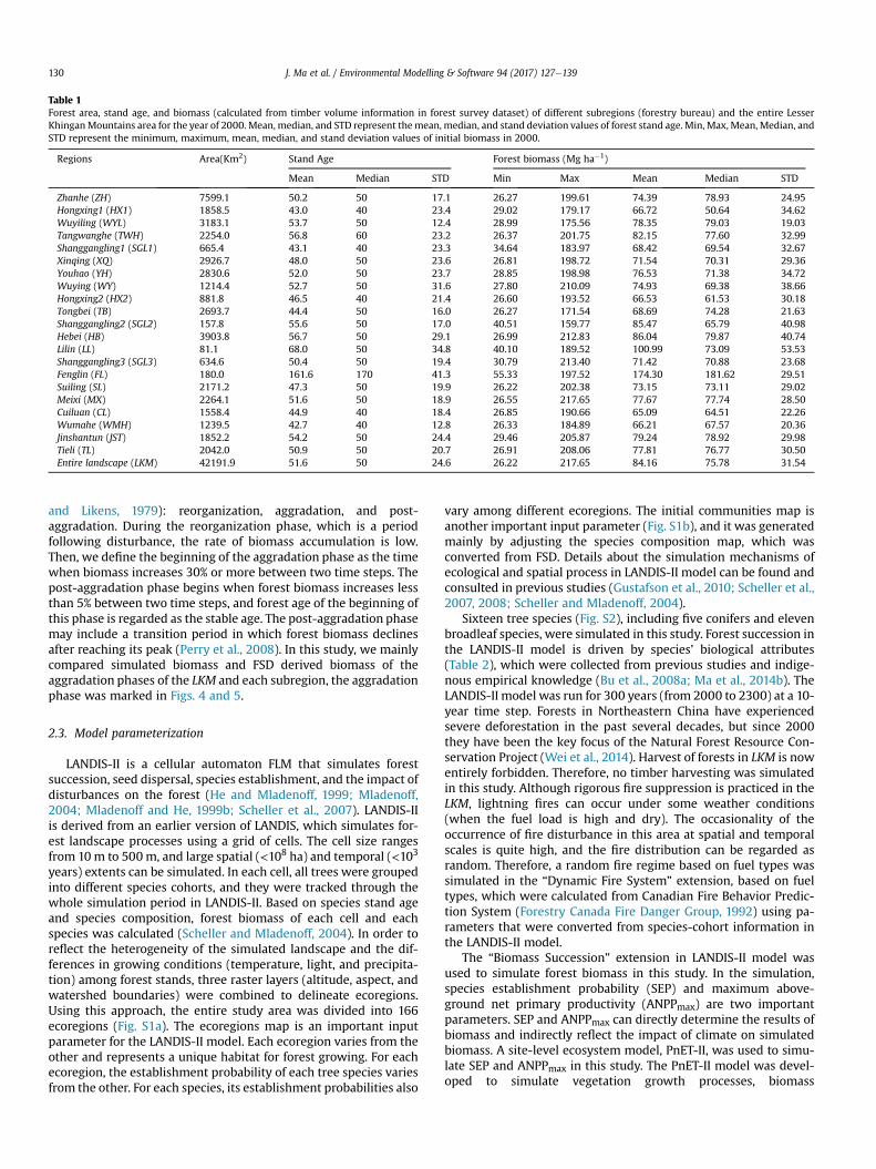
Table 1Forest area, stand age, and biomass (calculated from timber volume information in forest survey dataset) of different subregions (forestry bureau) and the entire LesserKhinganMountains area for the year of 2000. Mean, median, and STD represent themean, median, and stand deviation values of forest stand age. Min, Max, Mean, Median, andSTD represent the minimum, maximum, mean, median, and stand deviation values of initial biomass in 2000.

Regions Area(Km2) Stand Age Forest biomass (Mg ha�1)

Mean Median STD Min Max Mean Median STD

Zhanhe (ZH) 7599.1 50.2 50 17.1 26.27 199.61 74.39 78.93 24.95Hongxing1 (HX1) 1858.5 43.0 40 23.4 29.02 179.17 66.72 50.64 34.62Wuyiling (WYL) 3183.1 53.7 50 12.4 28.99 175.56 78.35 79.03 19.03Tangwanghe (TWH) 2254.0 56.8 60 23.2 26.37 201.75 82.15 77.60 32.99Shanggangling1 (SGL1) 665.4 43.1 40 23.3 34.64 183.97 68.42 69.54 32.67Xinqing (XQ) 2926.7 48.0 50 23.6 26.81 198.72 71.54 70.31 29.36Youhao (YH) 2830.6 52.0 50 23.7 28.85 198.98 76.53 71.38 34.72Wuying (WY) 1214.4 52.7 50 31.6 27.80 210.09 74.93 69.38 38.66Hongxing2 (HX2) 881.8 46.5 40 21.4 26.60 193.52 66.53 61.53 30.18Tongbei (TB) 2693.7 44.4 50 16.0 26.27 171.54 68.69 74.28 21.63Shanggangling2 (SGL2) 157.8 55.6 50 17.0 40.51 159.77 85.47 65.79 40.98Hebei (HB) 3903.8 56.7 50 29.1 26.99 212.83 86.04 79.87 40.74Lilin (LL) 81.1 68.0 50 34.8 40.10 189.52 100.99 73.09 53.53Shanggangling3 (SGL3) 634.6 50.4 50 19.4 30.79 213.40 71.42 70.88 23.68Fenglin (FL) 180.0 161.6 170 41.3 55.33 197.52 174.30 181.62 29.51Suiling (SL) 2171.2 47.3 50 19.9 26.22 202.38 73.15 73.11 29.02Meixi (MX) 2264.1 51.6 50 18.9 26.55 217.65 77.67 77.74 28.50Cuiluan (CL) 1558.4 44.9 40 18.4 26.85 190.66 65.09 64.51 22.26Wumahe (WMH) 1239.5 42.7 40 12.8 26.33 184.89 66.21 67.57 20.36Jinshantun (JST) 1852.2 54.2 50 24.4 29.46 205.87 79.24 78.92 29.98Tieli (TL) 2042.0 50.9 50 20.7 26.91 208.06 77.81 76.77 30.50Entire landscape (LKM) 42191.9 51.6 50 24.6 26.22 217.65 84.16 75.78 31.54

J. Ma et al. / Environmental Modelling & Software 94 (2017) 127e139130

and Likens, 1979): reorganization, aggradation, and post-aggradation. During the reorganization phase, which is a periodfollowing disturbance, the rate of biomass accumulation is low.Then, we define the beginning of the aggradation phase as the timewhen biomass increases 30% or more between two time steps. Thepost-aggradation phase begins when forest biomass increases lessthan 5% between two time steps, and forest age of the beginning ofthis phase is regarded as the stable age. The post-aggradation phasemay include a transition period in which forest biomass declinesafter reaching its peak (Perry et al., 2008). In this study, we mainlycompared simulated biomass and FSD derived biomass of theaggradation phases of the LKM and each subregion, the aggradationphase was marked in Figs. 4 and 5.

2.3. Model parameterization

LANDIS-II is a cellular automaton FLM that simulates forestsuccession, seed dispersal, species establishment, and the impact ofdisturbances on the forest (He and Mladenoff, 1999; Mladenoff,2004; Mladenoff and He, 1999b; Scheller et al., 2007). LANDIS-IIis derived from an earlier version of LANDIS, which simulates for-est landscape processes using a grid of cells. The cell size rangesfrom 10m to 500m, and large spatial (<108 ha) and temporal (<103

years) extents can be simulated. In each cell, all trees were groupedinto different species cohorts, and they were tracked through thewhole simulation period in LANDIS-II. Based on species stand ageand species composition, forest biomass of each cell and eachspecies was calculated (Scheller and Mladenoff, 2004). In order toreflect the heterogeneity of the simulated landscape and the dif-ferences in growing conditions (temperature, light, and precipita-tion) among forest stands, three raster layers (altitude, aspect, andwatershed boundaries) were combined to delineate ecoregions.Using this approach, the entire study area was divided into 166ecoregions (Fig. S1a). The ecoregions map is an important inputparameter for the LANDIS-II model. Each ecoregion varies from theother and represents a unique habitat for forest growing. For eachecoregion, the establishment probability of each tree species variesfrom the other. For each species, its establishment probabilities also

vary among different ecoregions. The initial communities map isanother important input parameter (Fig. S1b), and it was generatedmainly by adjusting the species composition map, which wasconverted from FSD. Details about the simulation mechanisms ofecological and spatial process in LANDIS-II model can be found andconsulted in previous studies (Gustafson et al., 2010; Scheller et al.,2007, 2008; Scheller and Mladenoff, 2004).

Sixteen tree species (Fig. S2), including five conifers and elevenbroadleaf species, were simulated in this study. Forest succession inthe LANDIS-II model is driven by species’ biological attributes(Table 2), which were collected from previous studies and indige-nous empirical knowledge (Bu et al., 2008a; Ma et al., 2014b). TheLANDIS-II model was run for 300 years (from 2000 to 2300) at a 10-year time step. Forests in Northeastern China have experiencedsevere deforestation in the past several decades, but since 2000they have been the key focus of the Natural Forest Resource Con-servation Project (Wei et al., 2014). Harvest of forests in LKM is nowentirely forbidden. Therefore, no timber harvesting was simulatedin this study. Although rigorous fire suppression is practiced in theLKM, lightning fires can occur under some weather conditions(when the fuel load is high and dry). The occasionality of theoccurrence of fire disturbance in this area at spatial and temporalscales is quite high, and the fire distribution can be regarded asrandom. Therefore, a random fire regime based on fuel types wassimulated in the “Dynamic Fire System” extension, based on fueltypes, which were calculated from Canadian Fire Behavior Predic-tion System (Forestry Canada Fire Danger Group, 1992) using pa-rameters that were converted from species-cohort information inthe LANDIS-II model.

The “Biomass Succession” extension in LANDIS-II model wasused to simulate forest biomass in this study. In the simulation,species establishment probability (SEP) and maximum above-ground net primary productivity (ANPPmax) are two importantparameters. SEP and ANPPmax can directly determine the results ofbiomass and indirectly reflect the impact of climate on simulatedbiomass. A site-level ecosystem model, PnET-II, was used to simu-late SEP and ANPPmax in this study. The PnET-II model was devel-oped to simulate vegetation growth processes, biomass

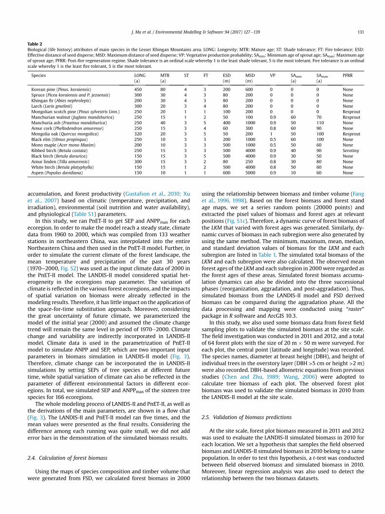
Table 2Biological (life history) attributes of main species in the Lesser Khingan Mountains area. LONG: Longevity; MTR: Mature age; ST: Shade tolerance; FT: Fire tolerance; ESD:Effective distance of seed disperse; MSD:Maximum distance of seed disperse; VP: Vegetative production probability; SAmin: Minimum age of sprout age; SAmax: Maximum ageof sprout age; PFRR: Post-fire regeneration regime. Shade tolerance is an ordinal scale whereby 1 is the least shade tolerant, 5 is the most tolerant. Fire tolerance is an ordinalscale whereby 1 is the least fire tolerant, 5 is the most tolerant.

Species LONG(a)

MTR(a)

ST FT ESD(m)

MSD(m)

VP SAmin

(a)SAmax

(a)PFRR

Korean pine (Pinus. koraiensis) 450 80 4 3 200 600 0 0 0 NoneSpruce (Picea koraiensis and P. jezoensis) 300 30 4 3 80 200 0 0 0 NoneKhingan fir (Abies nephrolepis) 200 30 4 3 80 200 0 0 0 NoneLarch (Larix gmelinii) 300 20 3 4 80 200 0 0 0 NoneMongolian scotch pine (Pinus sylvestris Linn.) 250 20 1 1 100 200 0 0 0 ResproutManchurian walnut (Juglans mandshurica) 250 15 1 2 50 100 0.9 60 70 ResproutManchuria ash (Fraxinus mandshurica) 250 40 3 5 400 1000 0.9 50 110 NoneAmur cork (Phellodendron amurense) 250 15 3 4 60 300 0.8 60 90 NoneMongolia oak (Quercus mongolica) 320 20 3 5 50 200 1 50 100 ResproutBlack elm (Ulmus propinqua) 250 10 3 3 200 1000 0.5 60 100 NoneMono maple (Acer mono Maxim) 200 10 3 3 500 1000 0.5 50 60 NoneRibbed birch (Betula costata) 250 15 3 3 500 4000 0.9 40 90 SerotinyBlack birch (Betula davurica) 150 15 3 5 500 4000 0.9 30 50 NoneAmur linden (Tilla amurensis) 300 15 3 2 80 250 0.8 30 80 NoneWhite birch (Betula platyphylla) 150 15 1 2 500 4000 0.8 50 60 NoneAspen (Populus davidiana) 150 10 1 1 600 5000 0.9 10 60 None

J. Ma et al. / Environmental Modelling & Software 94 (2017) 127e139 131

accumulation, and forest productivity (Gustafson et al., 2010; Xuet al., 2007) based on climatic (temperature, precipitation, andirradiation), environmental (soil nutrition and water availability),and physiological (Table S1) parameters.

In this study, we ran PnET-II to get SEP and ANPPmax for eachecoregion. In order to make the model reach a steady state, climatedata from 1960 to 2000, which was compiled from 133 weatherstations in northeastern China, was interpolated into the entireNortheastern China and then used in the PnET-II model. Further, inorder to simulate the current climate of the forest landscape, themean temperature and precipitation of the past 30 years(1970e2000, Fig. S2) was used as the input climate data of 2000 inthe PnET-II model. The LANDIS-II model considered spatial het-erogeneity in the ecoregions map parameter. The variation ofclimate is reflected in the various forest ecoregions, and the impactsof spatial variation on biomass were already reflected in themodeling results. Therefore, it has little impact on the application ofthe space-for-time substitution approach. Moreover, consideringthe great uncertainty of future climate, we parameterized themodel of the initial year (2000) and assumed the climate changetrend will remain the same level in period of 1970e2000. Climatechange and variability are indirectly incorporated in LANDIS-IImodel. Climate data is used in the parametrization of PnET-IImodel to simulate ANPP and SEP, which are two important inputparameters in biomass simulation in LANDIS-II model (Fig. 3).Therefore, climate change can be incorporated the in LANDIS-IIsimulations by setting SEPs of tree species at different futuretime, while spatial variation of climate can also be reflected in theparameter of different environmental factors in different ecor-egions. In total, we simulated SEP and ANPPmax of the sixteen treespecies for 166 ecoregions.

The whole modeling process of LANIDS-II and PnET-II, as well asthe derivations of the main parameters, are shown in a flow chat(Fig. 3). The LANDIS-II and PnET-II model ran five times, and themean values were presented as the final results. Considering thedifference among each running was quite small, we did not adderror bars in the demonstration of the simulated biomass results.

2.4. Calculation of forest biomass

Using the maps of species composition and timber volume thatwere generated from FSD, we calculated forest biomass in 2000

using the relationship between biomass and timber volume (Fanget al., 1996, 1998). Based on the forest biomass and forest standage maps, we set a series random points (20000 points) andextracted the pixel values of biomass and forest ages at relevantpositions (Fig. S1c). Therefore, a dynamic curve of forest biomass ofthe LKM that varied with forest ages was generated. Similarly, dy-namic curves of biomass in each subregion were also generated byusing the same method. The minimum, maximum, mean, median,and standard deviation values of biomass for the LKM and eachsubregion are listed in Table 1. The simulated total biomass of theLKM and each subregion were also calculated. The observed meanforest ages of the LKM and each subregion in 2000were regarded asthe forest ages of these areas. Simulated forest biomass accumu-lation dynamics can also be divided into the three successionalphases (reorganization, aggradation, and post-aggradation). Thus,simulated biomass from the LANDIS-II model and FSD derivedbiomass can be compared during the aggradation phase. All thedata processing and mapping were conducted using “raster”package in R software and ArcGIS 10.3.

In this study, we also used some biomass data from forest fieldsampling plots to validate the simulated biomass at the site scale.The field investigation was conducted in 2011 and 2012, and a totalof 64 forest plots with the size of 20 m � 50 m were surveyed. Foreach plot, the central point (latitude and longitude) was recorded.The species names, diameter at breast height (DBH), and height ofindividual trees in the overstory layer (DBH >5 cm or height >2 m)were also recorded. DBH-based allometric equations from previousstudies (Chen and Zhu, 1989; Wang, 2006) were adopted tocalculate tree biomass of each plot. The observed forest plotbiomass was used to validate the simulated biomass in 2010 fromthe LANDIS-II model at the site scale.

2.5. Validation of biomass predictions

At the site scale, forest plot biomass measured in 2011 and 2012was used to evaluate the LANDIS-II simulated biomass in 2010 foreach location. We set a hypothesis that samples the field observedbiomass and LANDIS-II simulated biomass in 2010 belong to a samepopulation. In order to test this hypothesis, a t-test was conductedbetween field observed biomass and simulated biomass in 2010.Moreover, linear regression analysis was also used to detect therelationship between the two biomass datasets.

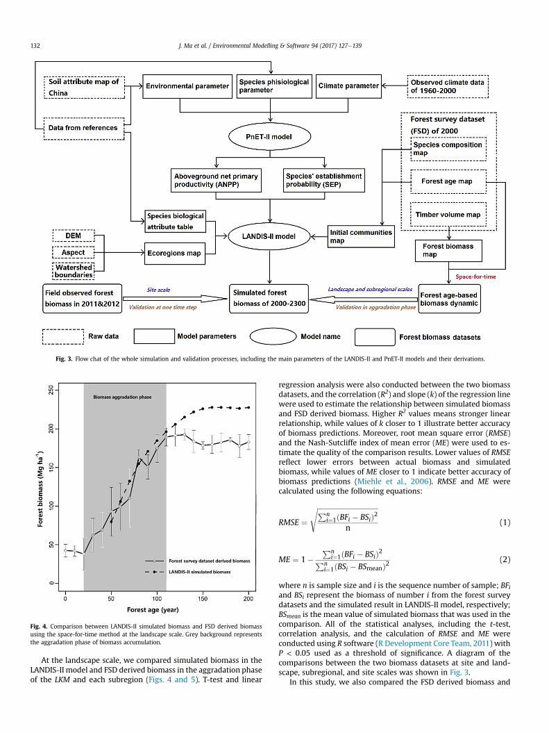
Fig. 3. Flow chat of the whole simulation and validation processes, including the main parameters of the LANDIS-II and PnET-II models and their derivations.

Fig. 4. Comparison between LANDIS-II simulated biomass and FSD derived biomassusing the space-for-time method at the landscape scale. Grey background representsthe aggradation phase of biomass accumulation.

J. Ma et al. / Environmental Modelling & Software 94 (2017) 127e139132

At the landscape scale, we compared simulated biomass in theLANDIS-II model and FSD derived biomass in the aggradation phaseof the LKM and each subregion (Figs. 4 and 5). T-test and linear

regression analysis were also conducted between the two biomassdatasets, and the correlation (R2) and slope (k) of the regression linewere used to estimate the relationship between simulated biomassand FSD derived biomass. Higher R2 values means stronger linearrelationship, while values of k closer to 1 illustrate better accuracyof biomass predictions. Moreover, root mean square error (RMSE)and the Nash-Sutcliffe index of mean error (ME) were used to es-timate the quality of the comparison results. Lower values of RMSEreflect lower errors between actual biomass and simulatedbiomass, while values of ME closer to 1 indicate better accuracy ofbiomass predictions (Miehle et al., 2006). RMSE and ME werecalculated using the following equations:

RMSE ¼ffiffiffiffiffiffiffiffiffiffiffiffiffiffiffiffiffiffiffiffiffiffiffiffiffiffiffiffiffiffiffiffiffiffiffiffiPn

i¼1ðBFi � BSiÞ2n

s(1)

ME ¼ 1�Pn

i¼1ðBFi � BSiÞ2Pni¼1ðBSi � BSmeanÞ2

(2)

where n is sample size and i is the sequence number of sample; BFiand BSi represent the biomass of number i from the forest surveydatasets and the simulated result in LANDIS-II model, respectively;BSmean is the mean value of simulated biomass that was used in thecomparison. All of the statistical analyses, including the t-test,correlation analysis, and the calculation of RMSE and ME wereconducted using R software (R Development Core Team, 2011) withP < 0.05 used as a threshold of significance. A diagram of thecomparisons between the two biomass datasets at site and land-scape, subregional, and site scales was shown in Fig. 3.

In this study, we also compared the FSD derived biomass and

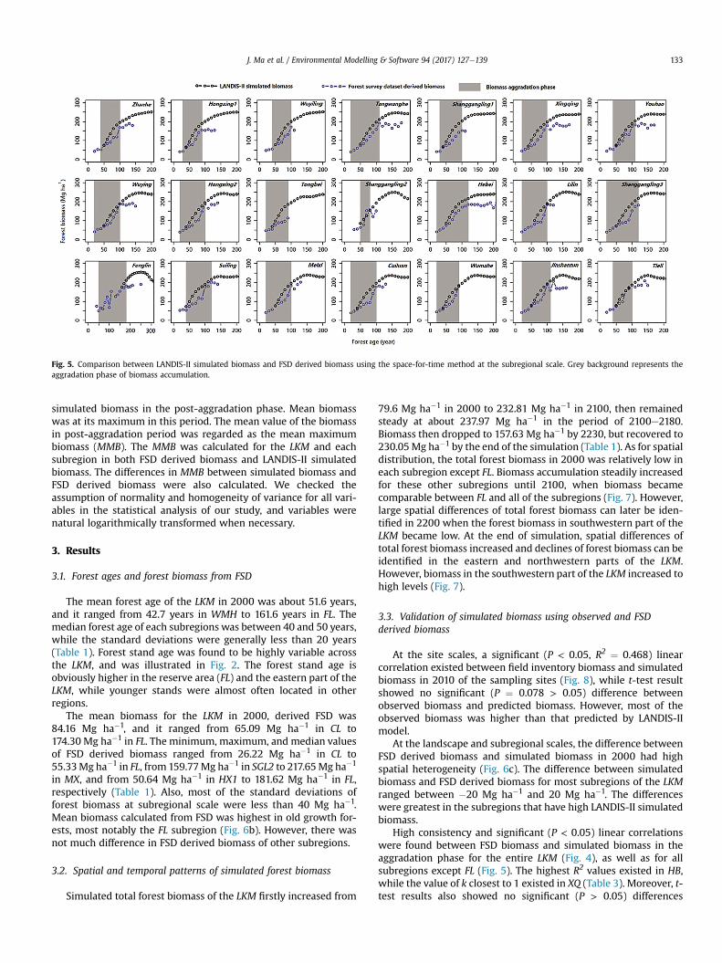
Fig. 5. Comparison between LANDIS-II simulated biomass and FSD derived biomass using the space-for-time method at the subregional scale. Grey background represents theaggradation phase of biomass accumulation.

J. Ma et al. / Environmental Modelling & Software 94 (2017) 127e139 133

simulated biomass in the post-aggradation phase. Mean biomasswas at its maximum in this period. The mean value of the biomassin post-aggradation period was regarded as the mean maximumbiomass (MMB). The MMB was calculated for the LKM and eachsubregion in both FSD derived biomass and LANDIS-II simulatedbiomass. The differences in MMB between simulated biomass andFSD derived biomass were also calculated. We checked theassumption of normality and homogeneity of variance for all vari-ables in the statistical analysis of our study, and variables werenatural logarithmically transformed when necessary.

3. Results

3.1. Forest ages and forest biomass from FSD

The mean forest age of the LKM in 2000 was about 51.6 years,and it ranged from 42.7 years in WMH to 161.6 years in FL. Themedian forest age of each subregions was between 40 and 50 years,while the standard deviations were generally less than 20 years(Table 1). Forest stand age was found to be highly variable acrossthe LKM, and was illustrated in Fig. 2. The forest stand age isobviously higher in the reserve area (FL) and the eastern part of theLKM, while younger stands were almost often located in otherregions.

The mean biomass for the LKM in 2000, derived FSD was84.16 Mg ha�1, and it ranged from 65.09 Mg ha�1 in CL to174.30 Mg ha�1 in FL. The minimum, maximum, and median valuesof FSD derived biomass ranged from 26.22 Mg ha�1 in CL to55.33Mg ha�1 in FL, from 159.77Mg ha�1 in SGL2 to 217.65Mg ha�1

in MX, and from 50.64 Mg ha�1 in HX1 to 181.62 Mg ha�1 in FL,respectively (Table 1). Also, most of the standard deviations offorest biomass at subregional scale were less than 40 Mg ha�1.Mean biomass calculated from FSD was highest in old growth for-ests, most notably the FL subregion (Fig. 6b). However, there wasnot much difference in FSD derived biomass of other subregions.

3.2. Spatial and temporal patterns of simulated forest biomass

Simulated total forest biomass of the LKM firstly increased from

79.6 Mg ha�1 in 2000 to 232.81 Mg ha�1 in 2100, then remainedsteady at about 237.97 Mg ha�1 in the period of 2100e2180.Biomass then dropped to 157.63 Mg ha�1 by 2230, but recovered to230.05Mg ha�1 by the end of the simulation (Table 1). As for spatialdistribution, the total forest biomass in 2000 was relatively low ineach subregion except FL. Biomass accumulation steadily increasedfor these other subregions until 2100, when biomass becamecomparable between FL and all of the subregions (Fig. 7). However,large spatial differences of total forest biomass can later be iden-tified in 2200 when the forest biomass in southwestern part of theLKM became low. At the end of simulation, spatial differences oftotal forest biomass increased and declines of forest biomass can beidentified in the eastern and northwestern parts of the LKM.However, biomass in the southwestern part of the LKM increased tohigh levels (Fig. 7).

3.3. Validation of simulated biomass using observed and FSDderived biomass

At the site scales, a significant (P < 0.05, R2 ¼ 0.468) linearcorrelation existed between field inventory biomass and simulatedbiomass in 2010 of the sampling sites (Fig. 8), while t-test resultshowed no significant (P ¼ 0.078 > 0.05) difference betweenobserved biomass and predicted biomass. However, most of theobserved biomass was higher than that predicted by LANDIS-IImodel.

At the landscape and subregional scales, the difference betweenFSD derived biomass and simulated biomass in 2000 had highspatial heterogeneity (Fig. 6c). The difference between simulatedbiomass and FSD derived biomass for most subregions of the LKMranged between �20 Mg ha�1 and 20 Mg ha�1. The differenceswere greatest in the subregions that have high LANDIS-II simulatedbiomass.

High consistency and significant (P < 0.05) linear correlationswere found between FSD biomass and simulated biomass in theaggradation phase for the entire LKM (Fig. 4), as well as for allsubregions except FL (Fig. 5). The highest R2 values existed in HB,while the value of k closest to 1 existed in XQ (Table 3). Moreover, t-test results also showed no significant (P > 0.05) differences

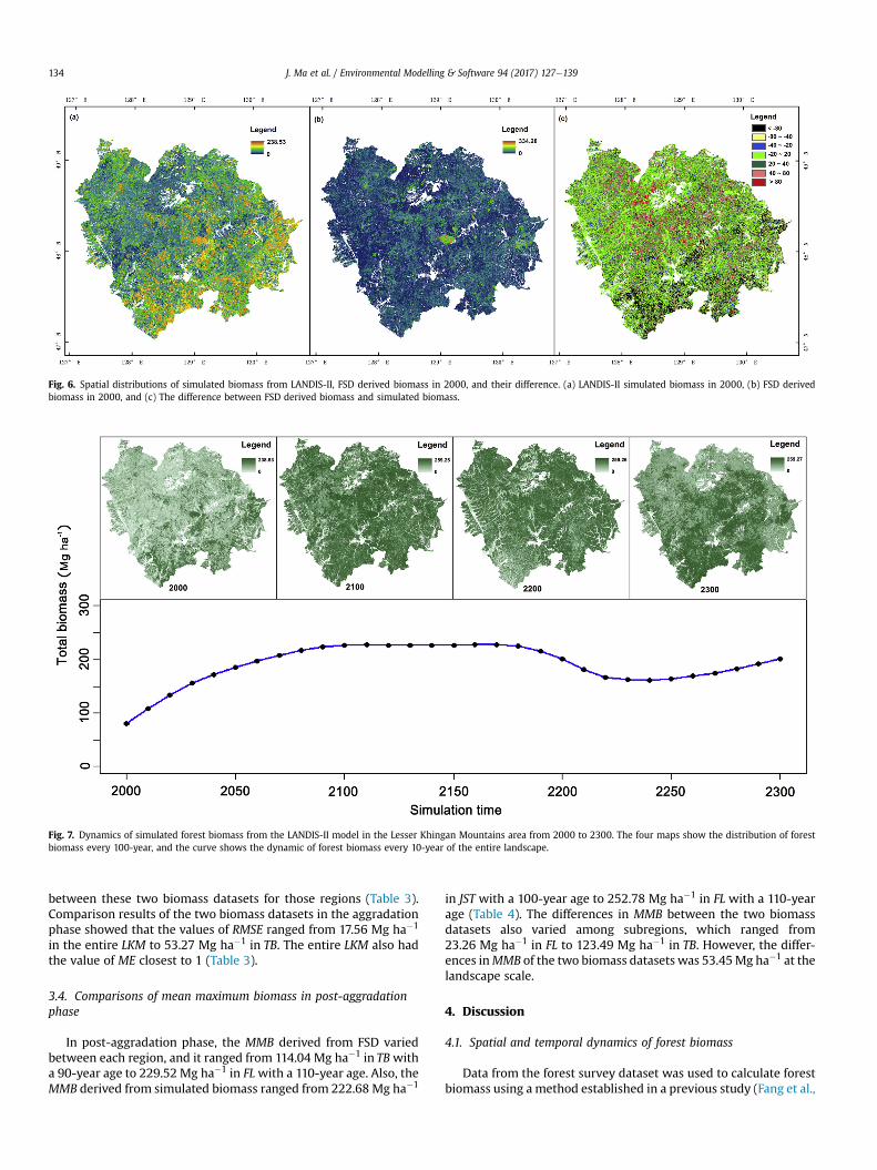
Fig. 6. Spatial distributions of simulated biomass from LANDIS-II, FSD derived biomass in 2000, and their difference. (a) LANDIS-II simulated biomass in 2000, (b) FSD derivedbiomass in 2000, and (c) The difference between FSD derived biomass and simulated biomass.

Fig. 7. Dynamics of simulated forest biomass from the LANDIS-II model in the Lesser Khingan Mountains area from 2000 to 2300. The four maps show the distribution of forestbiomass every 100-year, and the curve shows the dynamic of forest biomass every 10-year of the entire landscape.

J. Ma et al. / Environmental Modelling & Software 94 (2017) 127e139134

between these two biomass datasets for those regions (Table 3).Comparison results of the two biomass datasets in the aggradationphase showed that the values of RMSE ranged from 17.56 Mg ha�1

in the entire LKM to 53.27 Mg ha�1 in TB. The entire LKM also hadthe value of ME closest to 1 (Table 3).

3.4. Comparisons of mean maximum biomass in post-aggradationphase

In post-aggradation phase, the MMB derived from FSD variedbetween each region, and it ranged from 114.04 Mg ha�1 in TBwitha 90-year age to 229.52 Mg ha�1 in FLwith a 110-year age. Also, theMMB derived from simulated biomass ranged from 222.68 Mg ha�1

in JST with a 100-year age to 252.78 Mg ha�1 in FL with a 110-yearage (Table 4). The differences in MMB between the two biomassdatasets also varied among subregions, which ranged from23.26 Mg ha�1 in FL to 123.49 Mg ha�1 in TB. However, the differ-ences inMMB of the two biomass datasets was 53.45Mg ha�1 at thelandscape scale.

4. Discussion

4.1. Spatial and temporal dynamics of forest biomass

Data from the forest survey dataset was used to calculate forestbiomass using a method established in a previous study (Fang et al.,

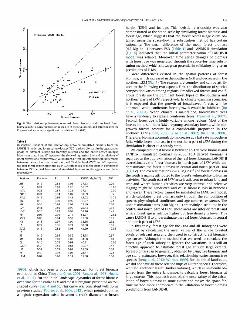
Fig. 8. The relationship between observed forest biomass and simulated forestbiomass in 2010. Linear regression is used to fit the relationship, and asterisks after theR square values indicate significant correlations (P < 0.05).

Table 3Descriptive statistics of the relationship between simulated biomass from theLANDIS-II model and forest survey dataset (FSD) derived biomass in the aggradationphase of different subregions (forestry bureau) and the entire Lesser KhinganMountains area. k and R2 represent the slope of regression line and correlations oflinear regressions, respectively. P-values from a t-test indicate significant differencesbetween the two biomass datasets at the 0.05 alpha level. RMSE and ME representthe root mean square error and Nash-Sutcliffe index of mean error in comparisonbetween FSD derived biomass and simulated biomass in the aggradation phase,respectively.

Regions P-values R2 k RMSE (Mg ha�1) ME

ZH 0.16 0.88 1.08 37.53 0.20HX1 0.24 0.89 1.20 35.37 �0.05WYL 0.21 0.85 1.23 37.21 �0.30TWH 0.24 0.94 1.07 31.89 0.35SGL1 0.13 0.94 1.43 42.02 �0.74XQ 0.19 0.90 0.99 36.27 0.22YH 0.36 0.93 1.04 25.49 0.60WY 0.41 0.89 0.90 25.63 0.61HX2 0.26 0.87 0.93 33.10 0.41TB 0.06 0.91 2.17 53.27 �7.63SGL2 0.86 0.84 0.53 18.68 0.71HB 0.18 0.97 1.09 32.56 0.32LL 0.22 0.76 0.71 37.90 0.01SGL3 0.16 0.82 1.08 41.29 �0.02FL e e e e e

SL 0.16 0.86 0.86 38.98 0.37MX 0.21 0.89 1.02 34.98 0.40CL 0.16 0.79 0.98 40.21 �0.06WMH 0.36 0.81 0.84 30.37 0.47JST 0.31 0.79 0.92 31.69 0.30TL 0.40 0.92 1.05 23.87 0.72LKM 0.67 0.90 1.14 17.56 0.76

J. Ma et al. / Environmental Modelling & Software 94 (2017) 127e139 135

1996), which has been a popular approach for forest biomassestimation in China (Fang and Chen, 2001; Fang et al., 1998; Huanget al., 2007). For the initial landscape, dynamics of forest biomassover time for the entire LKM andmost subregions presented an “S”-shaped curve (Figs. 4 and 5). This curve was consistent with someprevious studies (Poorter et al., 2006, 2012), which pointed out thata logistic regression exists between a tree's diameter at breast

height (DBH) and its age. This logistic relationship was alsodemonstrated at the stand scale by simulating forest biomass andforest age, which suggests that the forest biomass-age curve ob-tained using the space-for-time substitution method has certainrationality. The small difference of the mean forest biomass(4.6 Mg ha�1) between FSD (Table 1) and LANDIS-II simulation(Fig. 4) indicated that the initial parameterization of LANDIS-IImodel was reliable. Moreover, time series changes of biomasswith forest age was generated through the space-for-time substi-tutionmethod, which shows great potential in validating long-termpredictions of FLMs.

Great differences existed in the spatial patterns of forestbiomass, which increased in the southern LKM and decreased in thenorthern LKM (Fig. 7). The reasons are complex and can be attrib-uted to the following two aspects. First, the distribution of speciescomposition varies among regions. Broadleaved forests and conif-erous forests are the dominant forest types of the southern andnorthern parts of LKM, respectively. In climate warming scenarios,it is expected that the growth of broadleaved forests will beenhanced while coniferous forest growth would be inhibited (Buet al., 2008a). When climate is maintained, broadleaved treeshave a tendency to replace coniferous trees (Fraser et al., 2007).Second, forest age is highly variable among regions. Most of theforests in the southern LKM are young secondary forests, while old-growth forests account for a considerable proportion in thenorthern LKM (Chen, 2003; Xiao et al., 2002; Xu et al., 2008).Therefore, biomass accumulation increases at a fast rate in southernLKM, while forest biomass in the northern part of LKM during thesimulation is closer to a steady state.

We compared forest biomass between FSD derived biomass andLANDIS-II simulated biomass in 2000. FSD derived biomass isregarded as the approximation of the real forest biomass. LANDIS-IIoverestimates the forest biomass in north part of LKM while un-derestimates the forest biomass in central and north part of LKM(Fig. 6c). The overestimation (<�80 Mg ha�1) of forest biomass inthe south is mainly attributed to the forest's vulnerability to humanactivities. The south part of LKM area is adjacent to urban land andcropland where human activities are very intense, and selectivelogging might be conducted and cause biomass loss in branchesand leaves. These factors cannot be simulated in LANDIS-II model,which calculates forest biomass only through the composition ofspecies physiological conditions and age cohorts' existence. Theunderestimation areas (>80 Mg ha�1) are mainly distributed in thecentral and north part of LKM. These areas are interior forest landwhere forest age is relative higher but tree density is lower. Thiscause LANDIS-II to underestimate the real forest biomass in centraland north part of LKM.

In this study, forest age for the LKM and all subregions wereobtained by calculating the mean values of the whole forestedpixels of relevant area and then used to construct forest biomass-age curves. Although the method that we used to calculate theforest age of each subregion ignored the variations, it is still aneffective approach to estimate forest age at such large extents.Forest biomass can be generally obtained by using tree biomass andage stand estimates, however, this relationship varies among treespecies (Deng et al., 2012; Worbes, 1999). For the initial landscape,we did not have all these relationships of all tree species. Therefore,we used another dataset (timber volume), which is uniformly ob-tained from the entire landscape, to calculate forest biomass atlarge extents. This approach controls the uncertainty of the calcu-lation of forest biomass to some extent and makes the space-for-time method more appropriate in the validation of forest biomasspredictions from LANDIS-II.

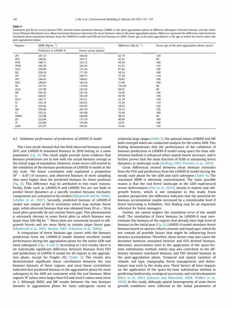
Table 4Simulated and forest survey dataset (FSD) derived mean maximum biomass (MMB) in the post-aggradation phase of different subregions (forestry bureau) and the entireLesser KhinganMountains area. Meanmaximum biomass represents the mean biomass value in the post-aggradation phase. Difference represent the difference value betweensimulated mean maximum biomass from the LANDIS-II model and FSD derived biomass in 2000. Forest age at the post-aggradation is the age at which the forest enters thepost-aggradation phase.

Regions MMB (Mg ha�1) Difference (Mg ha�1) Forest age at the post-aggradation phase (years)

Prediction in LANDIS-II Forest survey dataset

ZH 247.33 184.54 62.79 130HX1 246.62 154.71 91.91 90WYL 248.71 163.12 85.59 100TWH 243.78 182.26 61.52 110SGL1 239.06 151.24 87.82 100XQ 236.24 177.50 58.74 100YH 237.97 180.77 57.20 110WY 244.47 184.62 59.85 100HX2 240.02 182.54 57.48 100TB 237.53 114.04 123.49 90SGL2 237.49 143.24 94.25 80HB 234.76 181.10 53.66 120LL 244.07 183.29 60.78 100SGL3 242.71 181.61 61.10 120FL 252.78 229.52 23.26 110SL 224.36 195.93 28.43 120MX 236.06 201.94 34.12 130CL 233.52 181.08 52.44 100WMH 233.08 184.89 48.19 90JST 222.68 175.79 46.89 100TL 235.80 195.89 39.91 140LKM 237.97 184.52 53.45 120

J. Ma et al. / Environmental Modelling & Software 94 (2017) 127e139136

4.2. Validation performance of predictions of LANDIS-II model

The t-test result showed that the field observed biomass around2011 and LANDIS-II simulated biomass in 2010 belong to a samepopulation (Fig. 8). This result might provide some evidence thatbiomass predictions are in line with the actual biomass storage atthe initial stage of simulation. However, some errors still existed inthe validation of the biomass predictions of LANDIS-II model at thesite scale. The linear correlation only explained a proportion(R2 ¼ 0.47) of variance, and observed biomass of most samplingsites were higher than the predicted biomass for those positions(Fig. 8). This difference may be attributed to two main reasons.Firstly, FLMs such as LANDIS-II and LANDIS Pro are not built topredict forest dynamics at a specific location because stochasticcomponents are contained in themodels (Mladenoff and He,1999a;Scheller et al., 2007). Secondly, predicted biomass of LANDIS-IImodel was output at 90-m resolution which may include forestgaps, while observed biomass that was obtained from 20 m � 50 msized plots generally do not contain forest gaps. This phenomenonis extremely obvious in some forest plots in which biomass waslarger than 200 Mg ha�1. These plots are commonly located in old-growth forests and are more likely to contain larger forest gaps(Mladenoff et al., 1993; Runkle, 1981; Schnitzer et al., 2000).

A comparison of forest biomass-age curves with the biomasspredictions from the LANDIS-II model showed excellent modelperformance during the aggradation phase for the entire LKM andmost subregions (Figs. 4 and 5). According to t-test results, there isno statistically significant difference between biomass from FSDand predictions of LANDIS-II model for all regions in the aggrada-tion phase, except for Fenglin (FL) (Table 3). The results alsodemonstrated significant linear correlations between the twobiomass datasets of these regions, and most linear correlationsindicated that predicted biomass in the aggradation phase for mostsubregions in the LKM are consistent with the real biomass. Mostregions’ R2 values were larger than 0.8 andmost k values were closeto 1. Although RMSE and ME results between the two biomassdatasets in aggradation phase for most subregions varied in

relatively large ranges (Table 3), the optimal values of RMSE andMEboth emerged whenwe conducted analysis for the entire LKM. Thisfinding demonstrates that the performance of the validation ofbiomass predictions in LANDIS-II model using space-for-time sub-stitution method is enhanced when spatial extent increases, and itfurther proves that the main function of FLMs is simulating forestdynamics at landscape scale (Holling, 1992; Prentice et al., 1993).

Great differences existed between mean biomass estimatesfrom the FSD and predictions from the LANDIS-II model during thesteady state phase for the LKM and each subregion (Table 4). Thesimulated MMB is obviously overestimated. The main possiblereason is that the real forest landscape in the LKM experiencedsevere deforestation (Wei et al., 2014), mostly in mature and old-growth forests, which is not simulated in this study. Fromanother perspective, the difference indicates that the potential forbiomass accumulation maybe increased by a considerable level ifforest harvesting is forbidden. This finding may be an importantreference for forest managers.

Further, we cannot neglect the simulation error of the modelitself. The simulation of forest biomass by LANDIS-II may over-estimate the biomass of the regions that already have high level ofbiomass in the initial year (Fig. 6). LANDIS-II model simulates forestbiomass based on species cohorts amount and stand ages, which donot contain all possible factors that might be influencing forestbiomass accumulation. Therefore, these factors may also cause thedeviation between simulated biomass and FSD derived biomass.Moreover, uncertainties exist in the application of the space-for-time substitution method, which may also contribute to the dif-ference between simulated biomass and FSD derived biomass inthe post-aggradation phase. Temporal and spatial variation ofclimate, soil type, topography, forest management, and distur-bances may exist in the study area. These factors all have impactson the application of the space-for-time substitution method inpredicting biodiversity, ecological succession, and soil development(Blois et al., 2013; Johnson and Miyanishi, 2008; Walker et al.,2010). In this study, although spatial heterogeneity of some forestgrowth conditions were reflected in the initial parameters of

J. Ma et al. / Environmental Modelling & Software 94 (2017) 127e139 137

LANDIS-II model, we cannot address all possible factors that mightbe influencing forest biomass accumulation in the simulation.

In the LKM, Fenglin (FL) is a natural reserve where the forestshave been protected since the 1950s. Forest age composition of thissubregion can sustainably remain constant, and the forest age aswell as the biomass of most forests there remain at their maximumlevel (Table 1). This steady-state situation prohibits the detection ofthe aggradation in this subregion, and the space-for-time substi-tution method is not suitable for validation in this area. Moreover,forests in FL are commonly regarded as the climax stage of forestsuccession and used as a peak reference of carbon storage of forestsof other places (Bu et al., 2008b; Zhou et al., 2007). This finding isdemonstrated by the result of MMB in this study (Table 4), and itinspires us that the forest reserve is an area not only for biodiversityprotection, but can also increase the carbon sink.

4.3. Implications of space-for-time substitution method

This study attempts to use the space-for-time substitutionmethod to validate biomass predictions of a FLM at landscape scale.Forest biomass-age dynamic curves were used to compare long-term biomass predictions of the LANDIS-II model for the LKM, theresults of which demonstrated an excellent applicability at thelandscape scale. Nonetheless, before the age of 100 years, departureof the simulated biomass from biomass derived from FSD still existsinmost subregions (Fig. 5). This divergencemay be attributed to thefollowing reason. The mean value of the forest stand age (Table 1)shows the general status of the forest age of a subregion. However,in order to match the time step of LANDIS-II (10 years) and to seteach pair of biomass samples from FSD and LANDIS-II at the sametime, the age of a subregion was set as integer times of 10 in thecomparisons between the two biomass datasets. This may be a bigproblem and lead to departures in the final comparison betweenthe two biomass datasets. If we horizontally move the start point ofthe biomass curve that was derived from FSD to the right position(mean forest stand age) as shown in Table 1, the departure may bereduced.

Our study is a new attempt to conduct validations of long-termpredictions of FLMs at large spatial extents when only limited forestinventory data is available. Although data assimilation has beenwidely adopted to validate and calibrate the results of site-scaleecological models (Luo et al., 2014; Niu et al., 2014; Peng et al.,2011), it is still hard to apply data ingestion to evaluate pre-dictions produced by landscape models due to a lack of long timeseries observation at the landscape scale. Moreover, forest in-ventory data in China is limited and commonly difficult to acquire.Thus, validating predictions of FLMs using the space-for-timesubstitution method is an appropriate approach in landscapeecology. It allows for the realistic comparison between observedresults and long-term predicted results.

In order to simulate the real future state of forest landscape inLKM, no disturbance (forest harvest is banned in this area since2000) was modeled in this study. However, historical disturbanceslike timber harvesting have a certain impact on current forests(Ghilardi et al., 2016; Law et al., 2004; Nepstad et al., 1999;Robichaud, 2000), and the effects of disturbances have beendescribed by many previous studies at the landscape scale(Johnstone et al., 2010; Luo et al., 2014). In this study, we speculatedthat deforestation of old-growth forests had decreased the MMB,however, the mechanism and the degree of impacts from har-vesting as well as other disturbances is still worth future study.

5. Conclusions

Biomass predictions from the LANDIS-II model from 2000 to

2300was comparedwith FSD derived forest biomass at subregionaland the landscape scales using the space-for-time substitutionmethod in forest landscape of the LKM. Although it is impossible toexclude the spatial heterogeneity of the entire LKM landscape andamong different subregions, the space-for-time substitutionmethod is still been proved to have potential in validating timeseries biomass predictions of a FLM when only limited forest in-ventory data is available. Especially in the aggradation phase, highconsistency exists between simulated biomass and FSD derivedbiomass. Moreover, predicted biomass at one time step is consis-tent with field observed biomass data at the site scale.

As to the heterogeneity of the biomass distribution of the initiallandscape, forest reserve subregion (FL) stores more biomass thanother areas of the LKM. The differences in species composition andforest age composition may cause great variation in biomass dis-tribution during the simulation. Despite the simulation error of themodel itself and the uncertainties in the application of space-for-time substitution method, considerable loss of biomass due tohistorical harvesting in LKM may be the most possible explanationof the difference between the mean maximum biomass of simu-lated biomass and FSD derived biomass.

Acknowledgements

This research was funded by Natural Science Foundation ofChina (41601181 and 41571408) and China Postdoctoral ScienceFoundation (2015M581519). We thank Yu Chang, Zaiping Xiong,and Miao Liu for their field work.

Appendix A. Supplementary data

Supplementary data related to this article can be found at http://dx.doi.org/10.1016/j.envsoft.2017.04.004.

References

Berec, L., Dolezal, P., Hais, M., 2013. Population dynamics of Ips typographus in theBohemian Forest (Czech Republic): validation of the phenology model PHENIPSand impacts of climate change. For. Ecol. Manag. 292, 1e9.

Birdsey, R., Pregitzer, K., Lucier, A., 2006. Forest carbon management in the UnitedStates: 1600-2100. J. Environ. Qual. 35 (4), 1461e1469.

Blanco, J.A., Seely, B., Welham, C., Kimmins, J.P., Seebacher, T.M., 2007. Testing theperformance of a forest ecosystem model (FORECAST) against 29 years of fielddata in a Pseudotsuga menziesii plantation. Can. J. For. Research-Revue Can. DeRecherche For. 37 (10), 1808e1820.

Blois, J.L., Williams, J.W., Fitzpatrick, M.C., Jackson, S.T., Ferrier, S., 2013. Space cansubstitute for time in predicting climate-change effects on biodiversity. Proc.Natl. Acad. Sci. U. S. A. 110 (23), 9374e9379.

Bormann, F.H., Likens, G.E., 1979. Catastrophic disturbance and the steady-state innorthern hardwood forests. Am. Sci. 67 (6), 660e669.

Bu, R., He, H.S., Hu, Y.M., Chang, Y., Larsen, D.R., 2008a. Using the LANDIS model toevaluate forest harvesting and planting strategies under possible warmingclimates in Northeastern China. For. Ecol. Manag. 254 (3), 407e419.

Bu, R.C., Chang, Y., Hu, Y.M., Li, X.Z., He, H.S., 2008b. Sensitivity of coniferous trees toenvironmental factors at different scales in the Small Xing'an Mountains, China.J. Plant Ecol. 32 (1), 80e87 (in Chinese).

Busing, R.T., Solomon, A.M., McKane, R.B., Burdick, C.A., 2007. Forest dynamics inOregon landscapes: evaluation and application of an individual-based model.Ecol. Appl. 17 (7), 1967e1981.

Chave, J., 1999. Study of structural, successional and spatial patterns in tropical rainforests using TROLL, a spatially explicit forest model. Ecol. Model. 124 (2e3),233e254.

Chen, C., Zhu, J., 1989. The Biomass Manual of Main Tree Species in NortheasternChina. China Forestry Press, Beijing.

Chen, Y., 2003. Current state and development trend of vegetation in the LesserKhingan Mountains area. North. Environ. 28 (2), 42e44 (in Chinese).

Chiang, J.-M., McEwan, R.W., Yaussy, D.A., Brown, K.J., 2008. The effects of pre-scribed fire and silvicultural thinning on the aboveground carbon stocks andnet primary production of overstory trees in an oak-hickory ecosystem insouthern Ohio. For. Ecol. Manag. 255 (5e6), 1584e1594.

Deng, H., Bu, R., Liu, X., He, W., Hu, Y., Huang, N., 2012. Simulating the effects offorestry classified management on forest biomass in Xiao Xing'an Mountains.Acta Ecol. Sin. 32 (21), 6679e6687 (in Chinese).

Dixon, R.K., Brown, S., Houghton, R.A., Solomon, A.M., Trexler, M.C., Wisniewski, J.,

J. Ma et al. / Environmental Modelling & Software 94 (2017) 127e139138

1994. Carbon pools and flux of global forest ecosystems. Science 263 (5144),185e190.

Dong, B., Feng, Z., Zhang, D., Yao, S., Sui, H., Wang, J., 2008. Construction Technologyof Digital and Three-dimensional Forest Form Map Based on GIS. J. Beijing For.Univ. vol. 30 (1), 143e146 (in Chinese).

Fang, J.Y., Chen, A.P., 2001. Dynamic forest biomass carbon pools in China and theirsignificance. Acta Bot. Sin. 43 (9), 967e973.

Fang, J.Y., Liu, G.H., Xu, S.L., 1996. Biomass and net production of forest vegetation inChina. Acta Ecol. Sin. 16 (5), 497e508 (in Chinese).

Fang, J.Y., Wang, G.G., Liu, G.H., Xu, S.L., 1998. Forest biomass of China: an estimatebased on the biomass-volume relationship. Ecol. Appl. 8 (4), 1084e1091.

Forestry Canada Fire Danger Group, 1992. In: Directorate, F.C.S.a.S.D. (Ed.), Devel-opment and Structure of the Canadian Forest Fire Behavior Prediction System.Information Report ST-x-3 (Ottawa, Ontario, Canada).

Fraser, S.E.M., Dytham, C., Mayhew, P.J., 2007. Determinants of parasitoid abundanceand diversity in woodland habitats. J. Appl. Ecol. 44 (2), 352e361.

Gardner, R.H., Urban, D.L., 2003. Model validation and testing: past lessons, presentconcerns, future prospects.

Ghilardi, A., Bailis, R., Mas, J.-F., Skutsch, M., Alexander Elvir, J., Quevedo, A.,Masera, O., Dwivedi, P., Drigo, R., Vega, E., 2016. Spatiotemporal modeling offuelwood environmental impacts: towards improved accounting for non-renewable biomass. Environ. Model. Softw. 82, 241e254.

Gustafson, E.J., Shifley, S.R., Mladenoff, D.J., Nimerfro, K.K., He, H.S., 2000. Spatialsimulation of forest succession and timber harvesting using LANDIS. Can. J. For.Research-Revue Can. De Recherche For. 30 (1), 32e43.

Gustafson, E.J., Shvidenko, A.Z., Sturtevant, B.R., Scheller, R.M., 2010. Predictingglobal change effects on forest biomass and composition in south-centralSiberia. Ecol. Appl. 20 (3), 700e715.

He, H.S., 2008. Forest landscape models: definitions, characterization, and classifi-cation. For. Ecol. Manag. 254 (3), 484e498.

He, H.S., Hao, Z.Q., Mladenoff, D.J., Shao, G.F., Hu, Y.M., Chang, Y., 2005. Simulatingforest ecosystem response to climate warming incorporating spatial effects innorth-eastern China. J. Biogeogr. 32 (12), 2043e2056.

He, H.S., Mladenoff, D.J., 1999. Spatially explicit and stochastic simulation of forest-landscape fire disturbance and succession. Ecology 80 (1), 81e99.

He, H.S., Mladenoff, D.J., Crow, T.R., 1999. Linking an ecosystem model and a land-scape model to study forest species response to climate warming. Ecol. Model.114 (2e3), 213e233.

Holling, C.S., 1992. Cross-scale morphology, geometry, and dynamics of ecosystems.Ecol. Monogr. 62 (4), 447e502.

Houghton, R.A., Hackler, J.L., 2000. Changes in terrestrial carbon storage in theUnited States. 1: the roles of agriculture and forestry. Glob. Ecol. Biogeogr. 9 (2),125e144.

Huang, C.-D., Yang, W.-Q., Tang, X., 2007. Spatiotemporal variation of carbon storagein forest vegetation in Sichuan Province. Chin. J. Appl. Ecol. 18 (12), 2687e2692.

Johnson, E.A., Miyanishi, K., 2008. Testing the assumptions of chronosequences insuccession. Ecol. Lett. 11 (5), 419e431.

Johnstone, J.F., Hollingsworth, T.N., Chapin III, F.S., Mack, M.C., 2010. Changes in fireregime break the legacy lock on successional trajectories in Alaskan borealforest. Glob. Change Biol. 16 (4), 1281e1295.

Keith, H., Mackey, B.G., Lindenmayer, D.B., 2009. Re-evaluation of forest biomasscarbon stocks and lessons from the world's most carbon-dense forests. Proc.Natl. Acad. Sci. U. S. A. 106 (28), 11635e11640.

Larsen, D.R., Dey, D.C., Faust, T., 2010. A stocking diagram for midwestern easterncottonwood-silver maple-american sycamore bottomland forests. North. J.Appl. For. 27 (4), 132e139.

Law, B.E., Turner, D., Campbell, J., Sun, O.J., Van Tuyl, S., Ritts, W.D., Cohen, W.B.,2004. Disturbance and climate effects on carbon stocks and fluxes acrossWestern Oregon USA. Glob. Change Biol. 10 (9), 1429e1444.

Li, C., Flannigan, M.D., Corns, I.G.W., 2000. Influence of potential climate change onforest landscape dynamics of west-central Alberta. Can. J. For. Research-RevueCan. De Recherche For. 30 (12), 1905e1912.

Luo, X., He, H.S., Liang, Y., Wang, W.J., Wu, Z., Fraser, J.S., 2014. Spatial simulation ofthe effect of fire and harvest on aboveground tree biomass in boreal forests ofNortheast China. Landsc. Ecol. 29 (7), 1187e1200.

Ma, J., Bu, R.C., Deng, H.W., Hu, Y.M., Qin, Q., Han, F.L., 2014a. Simulating climatechange effect on aboveground carbon sequestration rates of main broad-leavedtrees in the Small Khingan Mountains area, Northeast China. Chin. J. Appl. Ecol.25 (9), 1106e1116 (in Chinese).

Ma, J., Bu, R.C., Liu, M., Chang, Y., Qin, Q., Hu, Y.M., 2015. Ecosystem carbon storagedistribution between plant and soil in different forest types in NortheasternChina. Ecol. Eng. 81, 353e362.

Ma, J., Hu, Y., Bu, R., Chang, Y., Deng, H., Qin, Q., 2014b. Predicting impacts of climatechange on the aboveground carbon sequestration rate of a temperate forest innortheastern China. Plos One 9 (4).

Marcot, B.G., Steventon, J.D., Sutherland, G.D., McCann, R.K., 2006. Guidelines fordeveloping and updating Bayesian belief networks applied to ecologicalmodeling and conservation. Can. J. For. Research-Revue Can. De Recherche For.36 (12), 3063e3074.

McMahon, S.M., Parker, G.G., Miller, D.R., 2010. Evidence for a recent increase inforest growth. Proc. Natl. Acad. Sci. U. S. A. 107 (8), 3611e3615.

Miehle, P., Livesley, S.J., Li, C.S., Feikema, P.M., Adams, M.A., Arndt, S.K., 2006.Quantifying uncertainty from large-scale model predictions of forest carbondynamics. Glob. Change Biol. 12 (8), 1421e1434.

Mladenoff, D.J., 2004. LANDIS and forest landscape models. Ecol. Model. 180 (1),

7e19.Mladenoff, D.J., He, H.S., 1999a. Design and Behavior of LANDIS, an Objectoriented

Model of Forest Landscape Disturbance and Succession. Cambridge UniversityPress, Cambridge, UK.

Mladenoff, D.J., He, H.S., 1999b. Design, Behavior and Application of LANDIS, anObject Oriented Model of Forest Landscape Disturbance and Succession Cam-bridge University Press, Cambridge.

Mladenoff, D.J., White, M.A., Pastor, J., Crow, T.R., 1993. Comparing spatial pattern inunaltered old-growth and disturbed forest landscapes. Ecol. Appl. 3 (2),294e306.

Nepstad, D.C., Verissimo, A., Alencar, A., Nobre, C., Lima, E., Lefebvre, P.,Schlesinger, P., Potter, C., Moutinho, P., Mendoza, E., Cochrane, M., Brooks, V.,1999. Large-scale impoverishment of Amazonian forests by logging and fire.Nature 398 (6727), 505e508.

Niu, S.L., Luo, Y.Q., Dietze, M.C., Keenan, T.F., Shi, Z., Li, J.W., Chapin, F.S., 2014. Therole of data assimilation in predictive ecology. Ecosphere 5 (5).

Peng, C., Guiot, J., Wu, H., Jiang, H., Luo, Y., 2011. Integrating models with data inecology and palaeoecology: advances towards a model-data fusion approach.Ecol. Lett. 14 (5), 522e536.

Perry, D.A., Oren, R., Hart, S.C., 2008. Forest ecosystems. Johns Hopkins UniversityPress.

Poorter, H., Niklas, K.J., Reich, P.B., Oleksyn, J., Poot, P., Mommer, L., 2012. Biomassallocation to leaves, stems and roots: meta-analyses of interspecific variationand environmental control. New Phytol. 193 (1), 30e50.

Poorter, L., Bongers, L., Bongers, F., 2006. Architecture of 54 moist-forest tree spe-cies: traits, trade-offs, and functional groups. Ecology 87 (5), 1289e1301.

Prentice, I.C., Sykes, M.T., Cramer, W., 1993. A simulation-model for the transienteffects of climate change on forest landscapes. Ecol. Model. 65 (1e2), 51e70.

R Development Core Team, 2011. R: a language and environment for statisticalcomputing. R foundation for statistical computing, Vienna p.

Robichaud, P.R., 2000. Fire effects on infiltration rates after prescribed fire inNorthern Rocky Mountain forests, USA. J. Hydrology 231, 220e229.

Runkle, J.R., 1981. Gap regeneration in some old-growth forests of the eastern-united-states. Ecol. 62 (4), 1041e1051.

Saatchi, S.S., Harris, N.L., Brown, S., Lefsky, M., Mitchard, E.T.A., Salas, W., Zutta, B.R.,Buermann, W., Lewis, S.L., Hagen, S., Petrova, S., White, L., Silman, M., Morel, A.,2011. Benchmark map of forest carbon stocks in tropical regions across threecontinents. Proc. Natl. Acad. Sci. U. S. A. 108 (24), 9899e9904.

Scheller, R.M., Domingo, J.B., Sturtevant, B.R., Williams, J.S., Rudy, A., Gustafson, E.J.,Mladenoff, D.J., 2007. Design, development, and application of LANDIS-II, aspatial landscape simulation model with flexible temporal and spatial resolu-tion. Ecol. Model. 201 (3e4), 409e419.

Scheller, R.M., Hua, D., Bolstad, P.V., Birdsey, R.A., Mladenoff, D.J., 2011a. The effectsof forest harvest intensity in combination with wind disturbance on carbondynamics in Lake States Mesic Forests. Ecol. Model. 222 (1), 144e153.

Scheller, R.M., Mladenoff, D.J., 2004. A forest growth and biomass module for alandscape simulation model, LANDIS: design, validation, and application. Ecol.Model. 180 (1), 211e229.

Scheller, R.M., Van Tuyl, S., Clark, K., Hayden, N.G., Hom, J., Mladenoff, D.J., 2008.Simulation of forest change in the New Jersey Pine Barrens under current andpre-colonial conditions. For. Ecol. Manag. 255 (5e6), 1489e1500.

Scheller, R.M., Van Tuyl, S., Clark, K.L., Hom, J., La Puma, I., 2011b. Carbon seques-tration in the New Jersey pine barrens under different scenarios of fire man-agement. Ecosyst. 14 (6), 987e1004.

Schmitz, O.J., 1997. Press perturbations and the predictability of ecological in-teractions in a food web. Ecol. 78 (1), 55e69.

Schnitzer, S.A., Dalling, J.W., Carson, W.P., 2000. The impact of lianas on treeregeneration in tropical forest canopy gaps: evidence for an alternativepathway of gap-phase regeneration. J. Ecol. 88 (4), 655e666.

Shifley, S.R., Rittenhouse, C.D., Millspaugh, J.J., Millspaugh, J.J., Thompson, F.R., 2009.Validation of landscape-scale decision support models that predict vegetationand wildlife dynamics.

Tian, S., Youssef, M.A., Chescheir, G.M., Skaggs, R.W., Cacho, J., Nettles, J., 2016.Development and preliminary evaluation of an integrated field scale model forperennial bioenergy grass ecosystems in lowland areas. Environ. Model. Softw.84, 226e239.

Tsoar, A., Allouche, O., Steinitz, O., Rotem, D., Kadmon, R., 2007. A comparativeevaluation of presence-only methods for modelling species distribution. Divers.Distrib. 13 (4), 397e405.

Walker, L.R., Wardle, D.A., Bardgett, R.D., Clarkson, B.D., 2010. The use of chro-nosequences in studies of ecological succession and soil development. J. Ecol.98 (4), 725e736.

Wang, C.K., 2006. Biomass allometric equations for 10 co-occurring tree species inChinese temperate forests. For. Ecol. Manag. 222 (1e3), 9e16.

Wang, F.G., Mladenoff, D.J., Forrester, J.A., Blanco, J.A., Scheller, R.M., Peckham, S.D.,Keough, C., Lucash, M.S., Gower, S.T., 2014a. Multimodel simulations of forestharvesting effects on long-term productivity and CN cycling in aspen forests.Ecol. Appl. 24 (6), 1374e1389.

Wang, W.J., He, H.S., Spetich, M.A., Shifley, S.R., Thompson III, F.R., Dijak, W.D.,Wang, Q., 2014b. A framework for evaluating forest landscape model pre-dictions using empirical data and knowledge. Environ. Model. Softw. 62,230e239.

Wei, Y.W., Zhou, W.M., Yu, D.P., Zhou, L., Fang, X.M., Zhao, W., Bao, Y., Meng, Y.Y.,Dai, L.M., 2014. Carbon storage of forest vegetation under the natural forestprotection program in northeast China. Acta Ecol. Sin. 34 (20), 5696e5705.

J. Ma et al. / Environmental Modelling & Software 94 (2017) 127e139 139

Worbes, M., 1999. Annual growth rings, rainfall-dependent growth and long-termgrowth patterns of tropical trees from the Caparo Forest Reserve inVenezuela. J. Ecol. 87 (3), 391e403.

Xiao, X.M., Boles, S., Liu, J.Y., Zhuang, D.F., Liu, M.L., 2002. Characterization of foresttypes in Northeastern China, using multi-temporal SPOT-4 VEGETATION sensordata. Remote Sens. Environ. 82 (2e3), 335e348.

Xu, C.-Y., Turnbull, M.H., Tissue, D.T., Lewis, J.D., Carson, R., Schuster, W.S.F.,Whitehead, D., Walcroft, A.S., Li, J., Griffin, K.L., 2012. Age-related decline ofstand biomass accumulation is primarily due to mortality and not to reductionin NPP associated with individual tree physiology, tree growth or stand struc-ture in a Quercus-dominated forest. J. Ecol. 100 (2), 428e440.

Xu, C.G., Gertner, G.Z., Scheller, R.M., 2007. Potential effects of interaction betweenCO2 and temperature on forest landscape response to global warming. Glob.

Change Biol. 13 (7), 1469e1483.Xu, W.D., He, X.Y., Chen, W., Liu, C.F., Zhao, G.L., Zhou, Y., 2008. Ecological division of

vegetation in Northeastern China. Chin. J. Ecol. 27 (11), 1853e1860 (in Chinese).Zaniewski, A.E., Lehmann, A., Overton, J.M.C., 2002. Predicting species spatial dis-

tributions using presence-only data: a case study of native New Zealand ferns.Ecol. Model. 157 (2e3), 261e280.

Zhang, G., Wang, Q., Zhang, F., Wu, K., Cai, C., Zhang, M., Li, D., Zhao, Y., Yang, J., 2013.Criteria for establishment of soil family and soil series in Chinese soil taxonomy.Acta Pedol. Sin. 50 (4), 826e834.

Zhou, D.H., He, H.S., Li, X.Z., Zhou, C.H., Wang, X.G., Chen, H.W., 2007. Potentialresponse of different stand age classes to climate change in the Xiao Xing'anMountains, northeastern China. J. Beijing For. Univ. 29 (4), 110e117 (in Chinese).