Applications of radium isotopes to ocean studies

Willard S. Moore University of South Carolina

Department of Earth and Ocean Science Columbia, SC, USA

moore@geol.sc.edu

230Th 232Th

228Th 227Th

226Ra 228Ra 224Ra 223Ra

1600 years 5.7 years 3.66 days 11.4 days

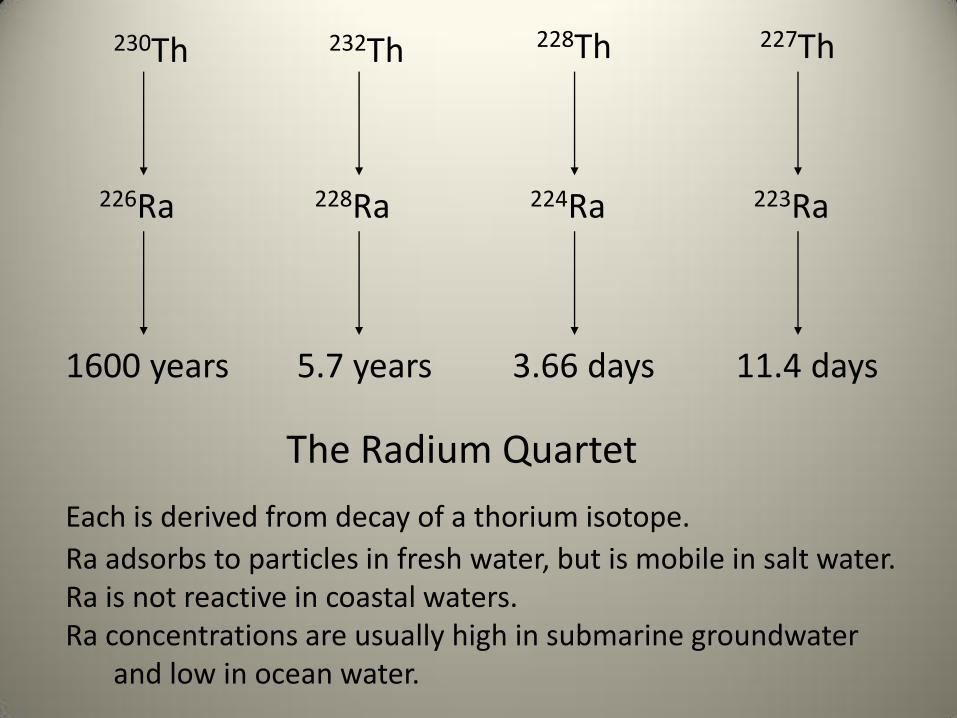
The Radium Quartet

Each is derived from decay of a thorium isotope.

Ra adsorbs to particles in fresh water, but is mobile in salt water. Ra is not reactive in coastal waters. Ra concentrations are usually high in submarine groundwater and low in ocean water.

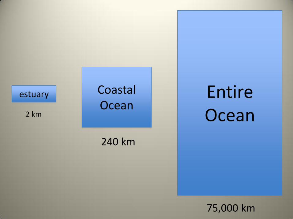
estuary Coastal Ocean

Entire Ocean 2 km

240 km

75,000 km

1. Flushing times in estuaries: Impact on biogeochemistry

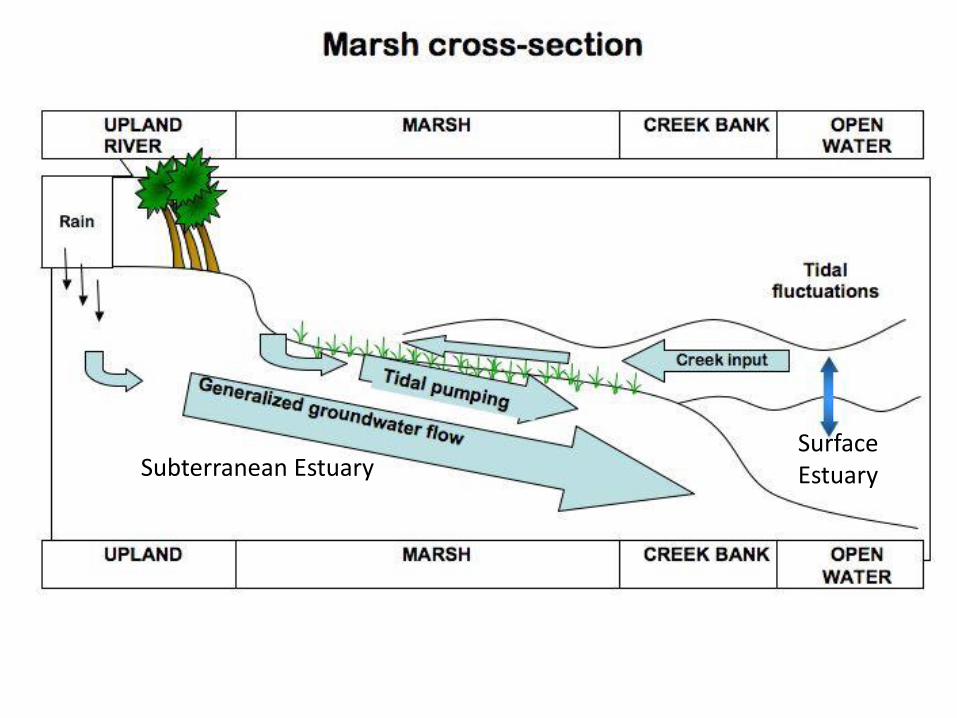
Subterranean Estuary Surface Estuary

Hypothesis: Mixtures of fresh groundwater and salty creek water react with marsh sediments. These biogeochemical reactions alter the composition of the groundwater and control fluxes of nutrients, carbon, and metals.

Estuary flushing time: ratio of the total mass divided by its rate of renewal.

Tf = total mass

rate of renewal

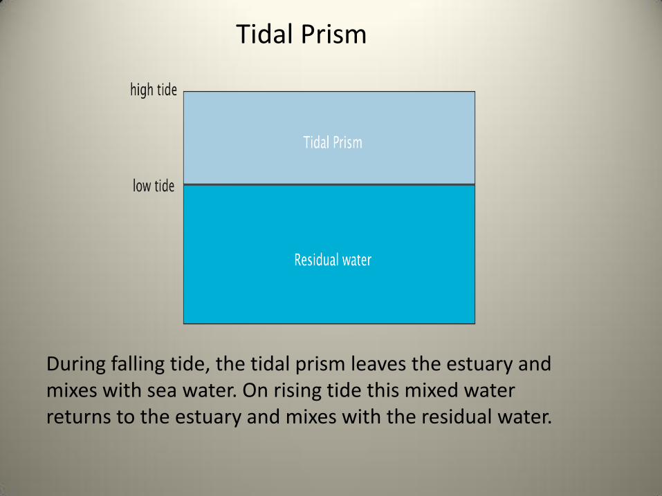
Tidal Prism

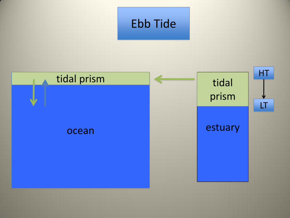
During falling tide, the tidal prism leaves the estuary and mixes with sea water. On rising tide this mixed water returns to the estuary and mixes with the residual water.

Tidal Prism

In the simplest application, the tidal prism that leaves the estuary is assumed to completely mix with sea water. On the rising tide this mixed water returns to the estuary and completely mixes with the residual water. Thus Tf = where V is volume of the estuary (average area x depth), T is the tidal period, 0.517 days, and P is the volume of the tidal prism. However, in most cases the assumption that the tidal prism mixes completely with sea water is not valid. This leads to an underestimation of Tf.

V T

P

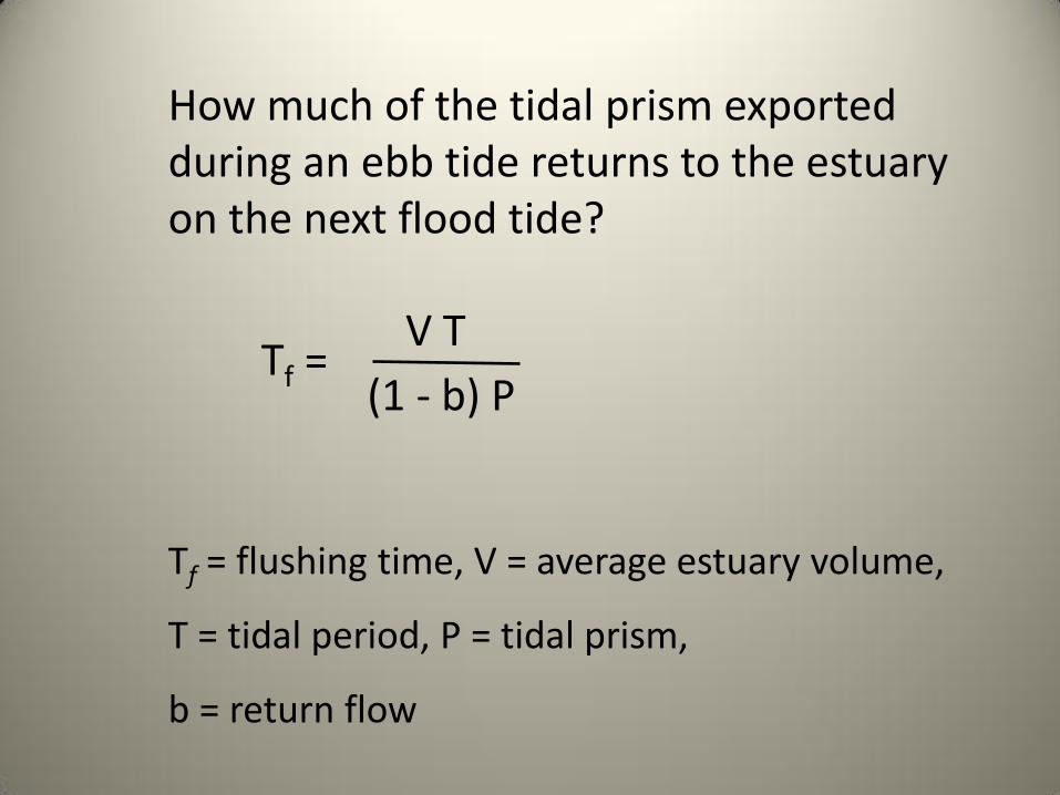
How much of the tidal prism exported during an ebb tide returns to the estuary on the next flood tide?

Tf = flushing time, V = average estuary volume,

T = tidal period, P = tidal prism,

b = return flow

Tf = V T

(1 - b) P

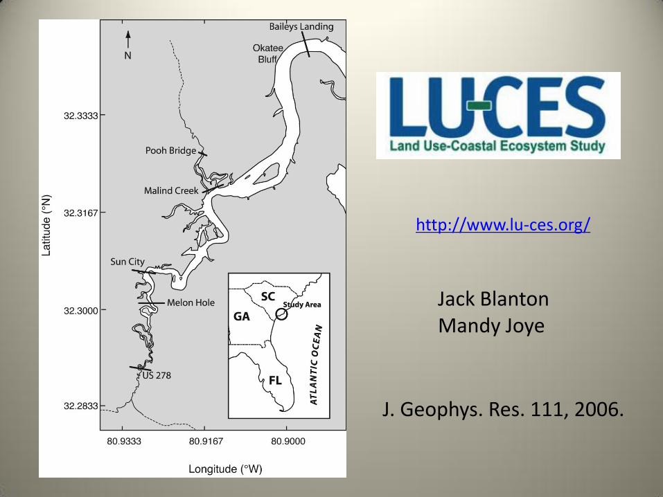
http://www.lu-ces.org/

Jack Blanton Mandy Joye

J. Geophys. Res. 111, 2006.

Tidal Prism

Physical oceanographers use differences between the outflowing tidal ebb velocity and the incoming flood velocity to determine b. This requires extensive knowledge of the estuary geometry and tidal currents. It produces a single value for b averaged over many tidal cycles.

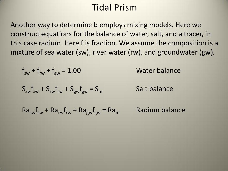
Tidal Prism Another way to determine b employs mixing models. Here we construct equations for the balance of water, salt, and a tracer, in this case radium. Here f is fraction. We assume the composition is a mixture of sea water (sw), river water (rw), and groundwater (gw). fsw + frw + fgw = 1.00 Water balance Sswfsw + Srwfrw + Sgwfgw = Sm Salt balance

Raswfsw + Rarwfrw + Ragwfgw = Ram Radium balance

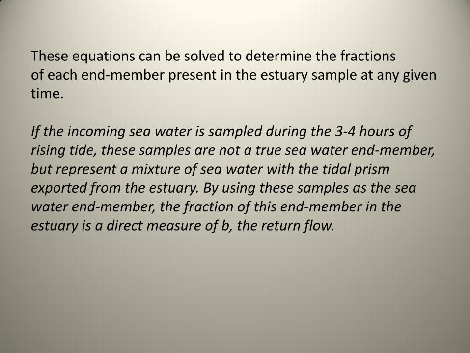
These equations can be solved to determine the fractions of each end-member present in the estuary sample at any given time. If the incoming sea water is sampled during the 3-4 hours of rising tide, these samples are not a true sea water end-member, but represent a mixture of sea water with the tidal prism exported from the estuary. By using these samples as the sea water end-member, the fraction of this end-member in the estuary is a direct measure of b, the return flow.

Ebb Tide

HT

LT

estuary

tidal prism

ocean

tidal prism

Flood Tide

HT

estuary ocean

partially-mixed tidal prism

LT

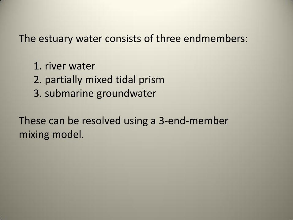
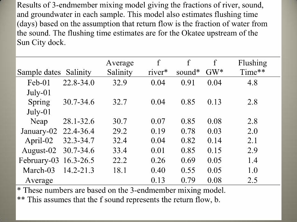
The estuary water consists of three endmembers: 1. river water 2. partially mixed tidal prism 3. submarine groundwater These can be resolved using a 3-end-member mixing model.

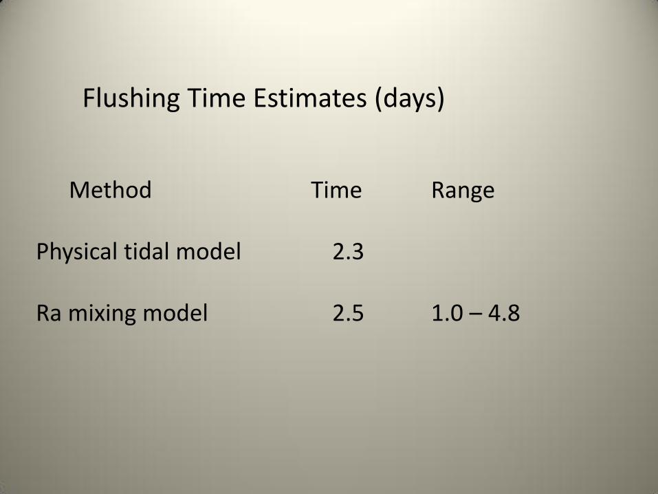
Flushing Time Estimates (days)

Method Time Range Physical tidal model 2.3 Ra mixing model 2.5 1.0 – 4.8

Primary source of nutrients and carbon to the surface estuary was submarine groundwater discharge.

2. Application of radium isotopes to study offshore mixing rates and submarine

groundwater discharge.

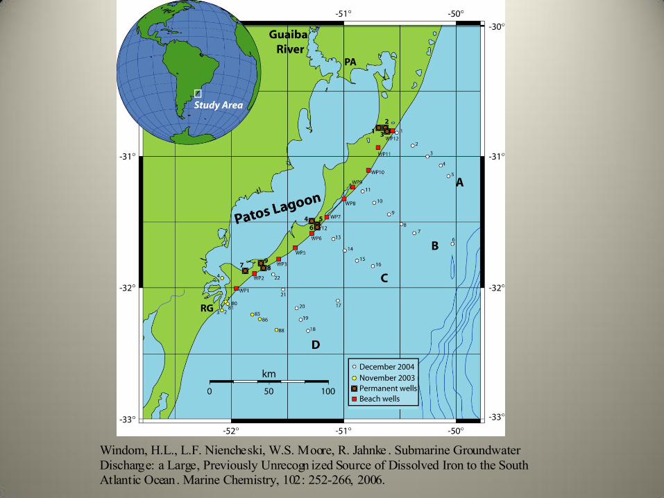
Windom, H.L., L.F. Niencheski, W.S. Moore, R. Jahnke . Submarine Groundwater

Discharge: a Large, Previously Unrecogn ized Source of Dissolved Iron to the South

Atlantic Ocean. Marine Chemistry, 102: 252-266, 2006.

•

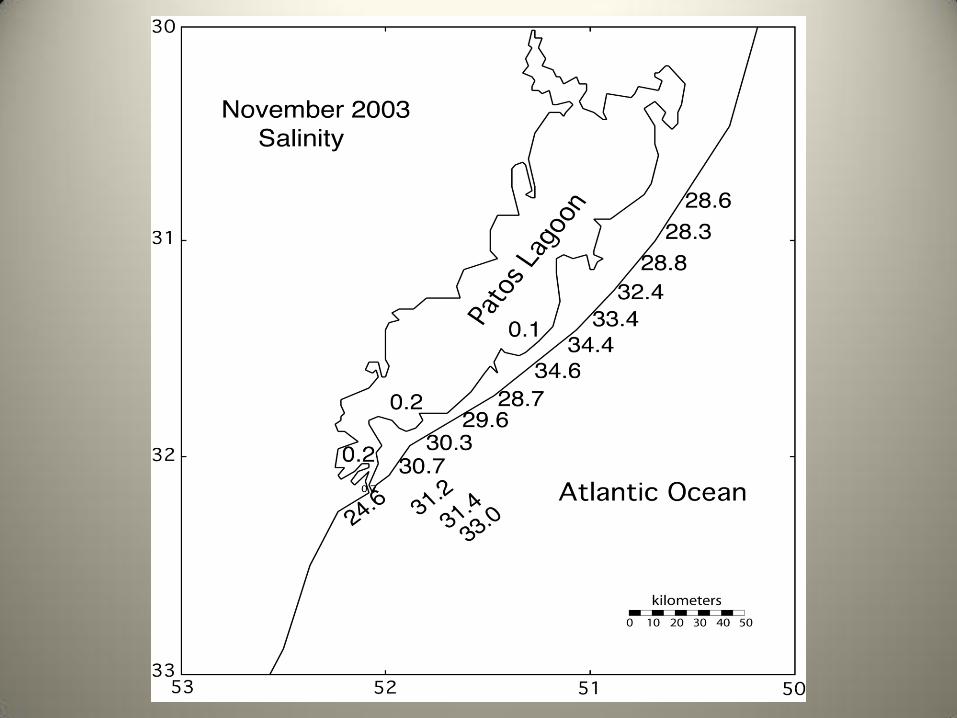
November 2003

plume

Lagoon maintains a positive head relative to the Atlantic. Sea level changes 2-3 m every 3-5 days due to wind setup.

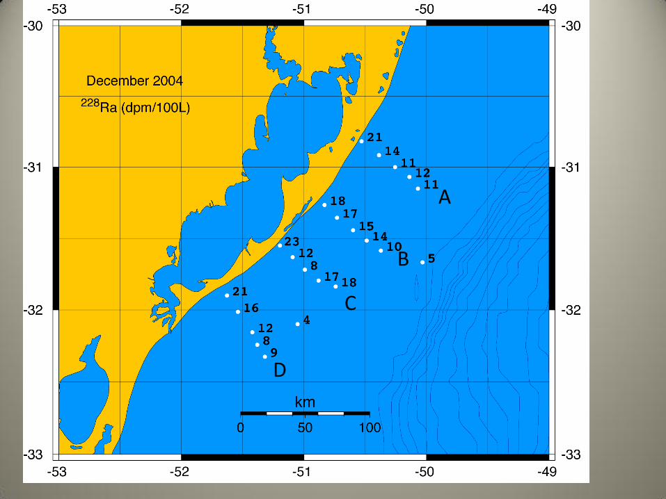
A

B

C

D

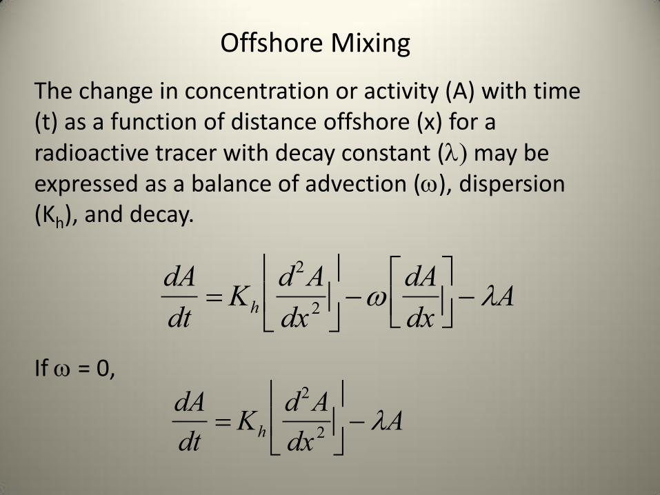
The change in concentration or activity (A) with time (t) as a function of distance offshore (x) for a radioactive tracer with decay constant ( may be expressed as a balance of advection (w), dispersion (Kh), and decay.

Offshore Mixing

If w = 0,

dA

dtKh

d2A

dx2

w

dA

dx

A

dA

dtKh

d2A

dx 2

A

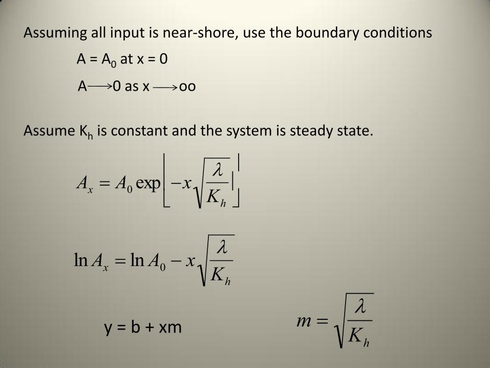
Assuming all input is near-shore, use the boundary conditions

Assume Kh is constant and the system is steady state.

A = A0 at x = 0 A 0 as x oo

y = b + xm

m

Kh

Ax A0 exp x

Kh

lnAx ln A0 x

Kh

The linear gradient implies that mixing, not advection, controls the distribution.

Kh (224) = 24 km2 day-1

Kh (224) = 19 km2 day-1

Kh (223) = 29 km2 day-1

Kh (223) = 29 km2 day-1

(29 km2 day-1 = 336 m2 s-1)

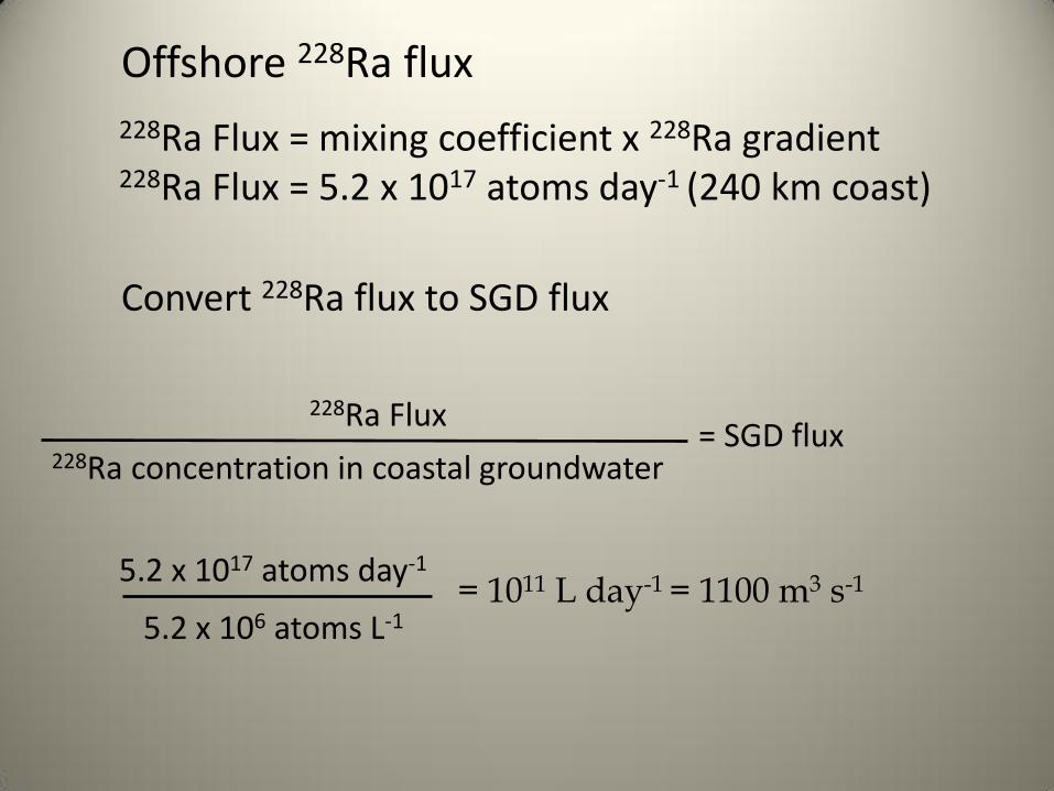
228Ra Flux = mixing coefficient x 228Ra gradient 228Ra Flux = 5.2 x 1017 atoms day-1 (240 km coast)

Offshore 228Ra flux

Convert 228Ra flux to SGD flux

5.2 x 1017 atoms day-1

5.2 x 106 atoms L-1 = 1011 L day-1 = 1100 m3 s-1

228Ra Flux 228Ra concentration in coastal groundwater

= SGD flux

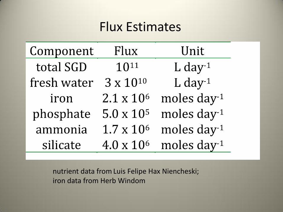
Flux Estimates

nutrient data from Luis Felipe Hax Niencheski; iron data from Herb Windom

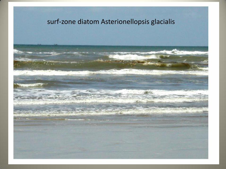
surf-zone diatom Asterionellopsis glacialis

With Kh = 29 km2 day-1,

L 2Kh

Define residence time as the time required to remove the water from 1/e of the width of the shelf. If we take the shelf width as 60 km, the length scale is 22 km. Use the Einstein equation to estimate residence time:

residence time = 8 days.

The SGD introduces a great deal of dissolved iron to the coastal water. How much Fe reaches the open ocean?

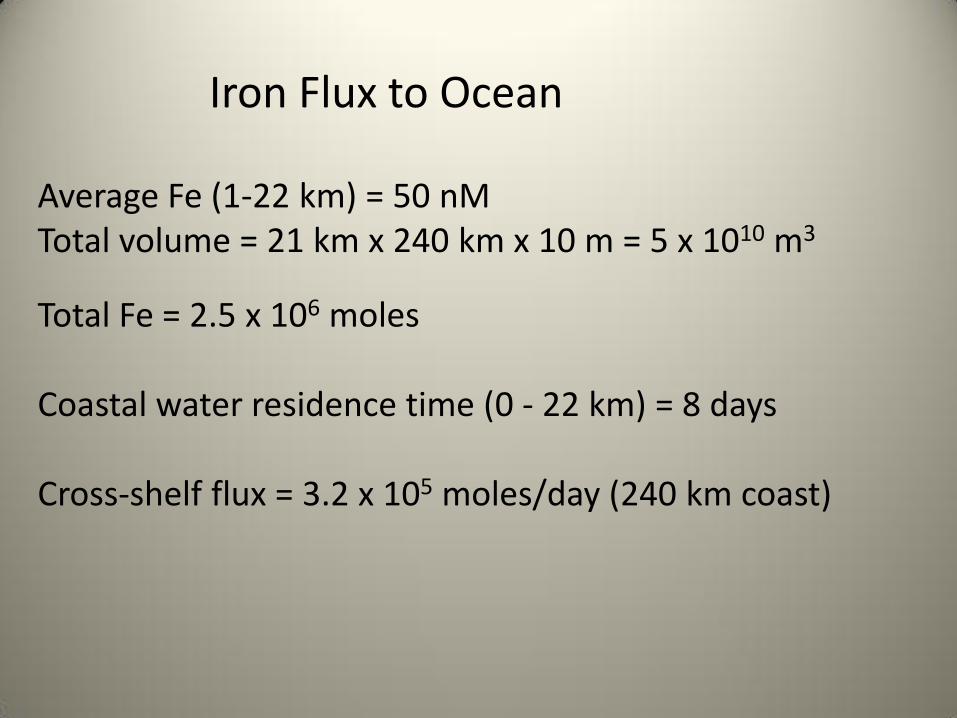
Iron Flux to Ocean

Average Fe (1-22 km) = 50 nM Total volume = 21 km x 240 km x 10 m = 5 x 1010 m3

Total Fe = 2.5 x 106 moles Coastal water residence time (0 - 22 km) = 8 days Cross-shelf flux = 3.2 x 105 moles/day (240 km coast)

Comparison with Other Inputs to the South Atlantic

With Atmospheric Deposition:

Atmospheric Fe Flux = 0.2 µmol·m-2·y-1

Area of South Atlantic = 40 x 1012 m 2

Atmospheric Fe Flux = 2.2 x 106 mol·d-1

Cross-Shelf Fe Flux = 3.2 x 105 mol·d-1

Fe flux from this 240 km coastline is >10% of the total atmospheric Fe flux to the South Atlantic.

The first World Atlas of the artificial night sky brightness, P. Cinzano, F. Falchi, and C.D. Elvidge, Mon. Not. R. Astron. Soc. 328, 689-702, 2001.

3. How important is submarine groundwater discharge on a global scale?

Definition of SGD:

Submarine groundwater discharge (SGD) is the flow of water through continental margins from the seabed to the coastal ocean, with scale lengths of meters to kilometers, regardless of fluid composition or driving force.

It is important to recognize that SGD can be fresh or salty water and that the composition is usually very different from the water that entered the aquifer. SGD is typically enriched in nutrients, metals, and carbon as well as Ra.

This CRP led to 59

published papers as

of 2006.

232Th 228Ra

half life = 5.7 years = 0.12 yr-1

TTO 1981-1989

Bob Key, Jorge Sarmiento

Princeton

Nature Geoscience 1, 309-311, 2008.

Stations with 228Ra profiles

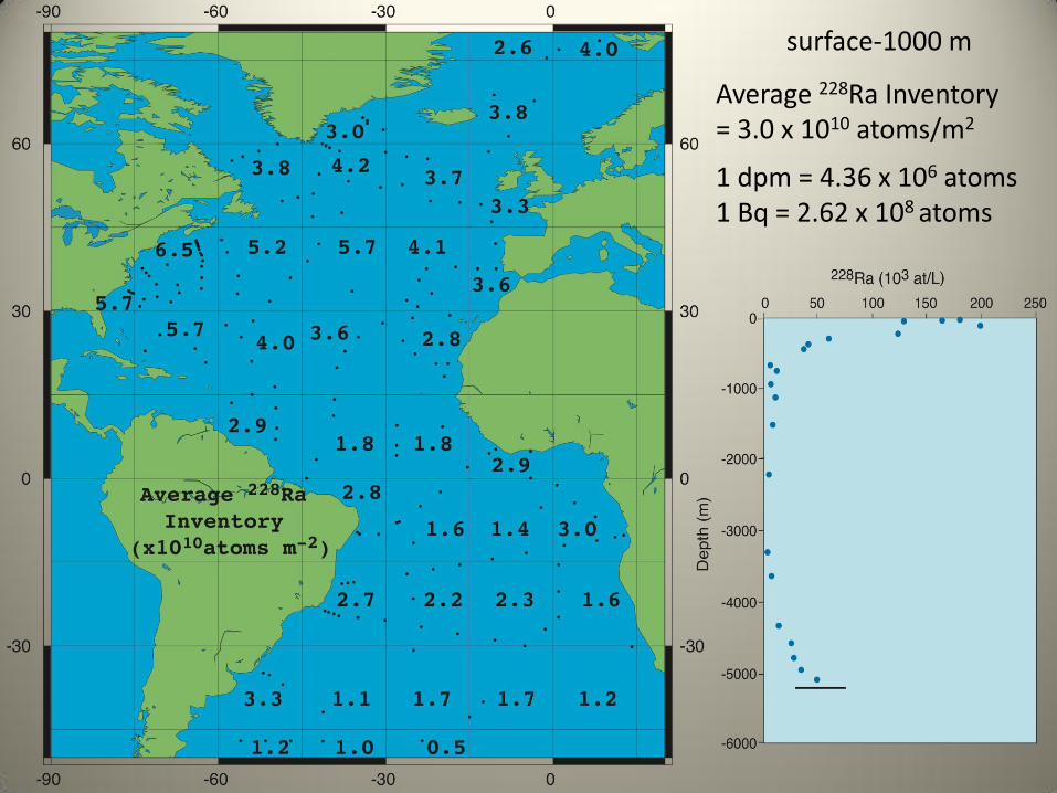
Average 228Ra Inventory = 3.0 x 1010 atoms/m2

surface-1000 m

1 dpm = 4.36 x 106 atoms 1 Bq = 2.62 x 108 atoms

Total inventory 228Ra = 2.9 x 1024 atoms in upper 1000 m

12% of the 228Ra inventory decays each year. This must be replaced by a similar flux from the continents to maintain steady state.

228Ra flux = 2.9 x 1024 atoms x 0.12 year-1

= 3.5 x 1023 atoms year-1

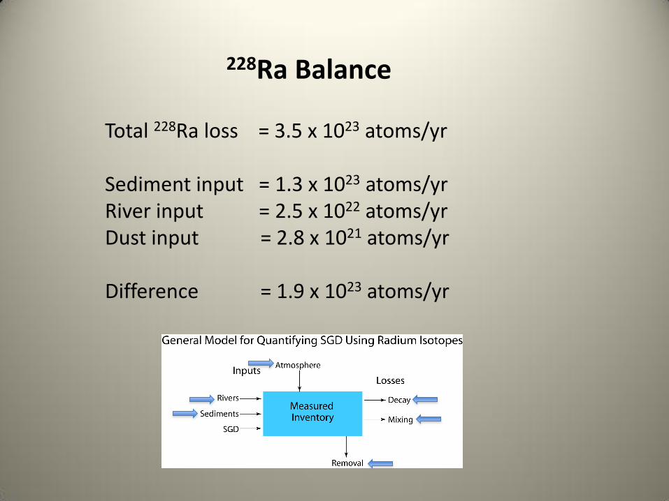
228Ra Balance

Total 228Ra loss = 3.5 x 1023 atoms/yr Sediment input = 1.3 x 1023 atoms/yr River input = 2.5 x 1022 atoms/yr Dust input = 2.8 x 1021 atoms/yr Difference = 1.9 x 1023 atoms/yr

228Ra Balance

Total 228Ra loss = 3.5 x 1023 atoms/yr Sediment input = 1.3 x 1023 atoms/yr River input = 2.5 x 1022 atoms/yr Dust input = 2.8 x 1021 atoms/yr Difference = 1.9 x 1023 atoms/yr

This must come from SGD.

Need the concentration of 228Ra in SGD to convert the 228Ra flux to the SGD flux.

SGD Flux (L/yr) = 228Ra Flux (atoms/year)

[228Ra]SGD (atoms/L)

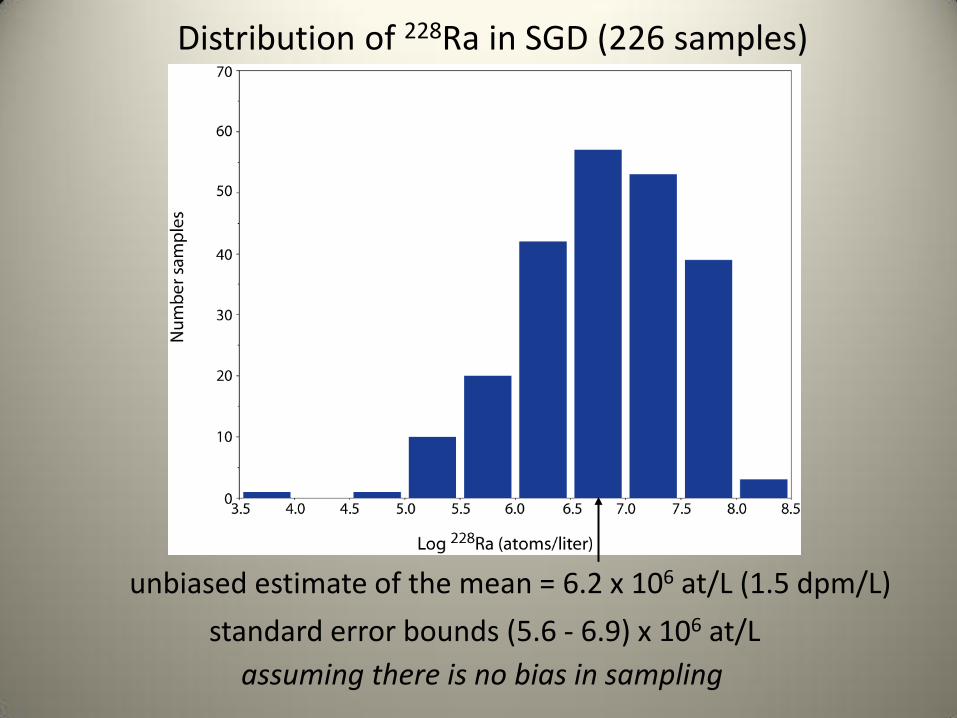
Distribution of 228Ra in SGD (226 samples)

unbiased estimate of the mean = 6.2 x 106 at/L (1.5 dpm/L)

standard error bounds (5.6 - 6.9) x 106 at/L

assuming there is no bias in sampling

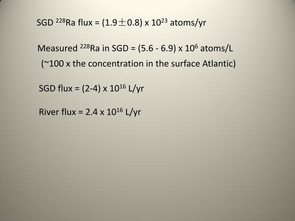
SGD 228Ra flux = (1.9±0.8) x 1023 atoms/yr

Measured 228Ra in SGD = (5.6 - 6.9) x 106 atoms/L

(~100 x the concentration in the surface Atlantic)

SGD flux = (2-4) x 1016 L/yr River flux = 2.4 x 1016 L/yr

How important is SGD on a global scale? The SGD flux to the Atlantic Ocean is similar to the river flux to the Atlantic (80-160% of the river flux).

Because SGD contains higher

concentrations of many components than

do rivers, this flux is probably more

important in maintaining the balance of

many elements in the ocean.

Comparison of large-scale SGD estimates

Region

Date Coast length

km

SGD Flux

108 L km-1 d-1

Reference

Onslow Bay Jul-02 140 8

McCoy et al.

2007

SAB Jul-94 320 7 Moore 2000

SAB Sep-98 600 13 Moore 2010

SAB Oct-98 600 9 Moore 2010

SAB Apr-99 600 12 Moore 2010

SAB Feb-00 600 6 Moore 2010

Patos Lagoon Dec-04 240 4

Windom et al.

2006

Atlantic 1981-1989 75,000 10

Moore et al.

2008

Conclusions

Because Ra isotopes have very different activities in river, estuary, ocean, and ground water, they provide an index of the mixing ratios of these components in estuarine and coastal waters.

By selecting the appropriate combination of Ra isotopes, time scales of estuary flushing and coastal mixing can be determined.

One of the most important outcomes of Ra isotope studies is that submarine groundwater discharge (SGD) has been recognized as an important component of the hydrologic cycle, rivaling rivers as a pathway for nutrient, carbon, and metal input to the ocean.

With this new understanding of time scales and fluxes in the near-shore environment, scientists and coastal managers are now able to evaluate sources of nutrients, carbon, and metals and their impact on the coastal ocean.

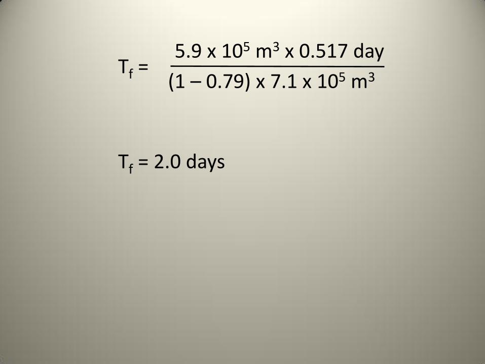
Tf = 5.9 x 105 m3 x 0.517 day

(1 – 0.79) x 7.1 x 105 m3

Tf = 2.0 days

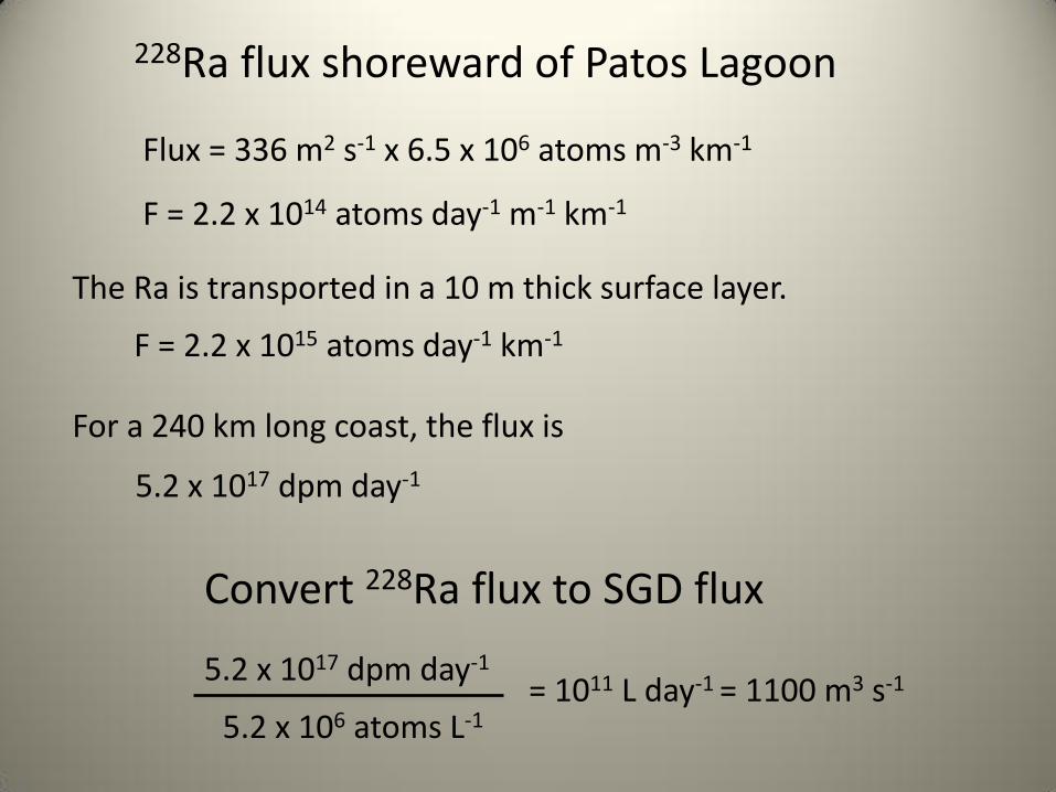
Flux = 336 m2 s-1 x 6.5 x 106 atoms m-3 km-1

F = 2.2 x 1014 atoms day-1 m-1 km-1

The Ra is transported in a 10 m thick surface layer.

F = 2.2 x 1015 atoms day-1 km-1

For a 240 km long coast, the flux is

5.2 x 1017 dpm day-1

228Ra flux shoreward of Patos Lagoon

Convert 228Ra flux to SGD flux

5.2 x 1017 dpm day-1

5.2 x 106 atoms L-1 = 1011 L day-1 = 1100 m3 s-1