Approaches to Item Scaling - Conservancy - University of Minnesota

451

Relationships Between the Thurstone and RaschApproaches to Item ScalingDavid AndrichThe University of Western Australia

When the logistic function is substituted for thenormal, Thurstone’s Case V specialization of thelaw of comparative judgment for paired comparisonresponses gives an identical equation for the esti-mation of item scale values as does the Raschformulation for direct responses. The law of com-

parative judgment must be modified to include asubject parameter; but this parameter, which is

eliminated statistically with respect to the direct re-sponse design, is eliminated experimentally in thepaired comparison design. Some comparisons andcontrasts are made between the two approaches toitem scaling, and it is shown that greater gen-eralizability for item scaling is possible when thetwo approaches are juxtaposed appropriately.

The application of Thurstone’s law of comparative judgment to items which have no physicalproperties (e.g., statements), permits identification of a conformable set of items which can then beused to measure subjects on a psychological continuum. More specifically, both the evidence that aset of items does refer to a unidimensional continuum and the relative scale values of the items are

provided.The basic data collection design for scaling items in the Thurstone tradition is that of paired

comparisons, while the most common design for measurement requires subjects to respond to itemsaccording to some positive-negative dichotomy, such as &dquo;agree&dquo; or &dquo;disagree.&dquo; To contrast this latterdesign with that of paired comparisons, it will be called the direct response design. Measurements ofsubjects are then usually the medians of the scale values of the items they endorse positively(Edwards, 1957).

An alternate approach to scaling items and measuring subjects is available from latent trait psy-chometric theory. Subjects who are to be measured respond according to the direct response design,but these same responses may be used both to scale items and to measure subjects. A number ofstatistical models have been proposed for transforming the responses to these two ends. One of thesimplest and most elegant ones is the Rasch (1960, 1961) simple logistic model (SLM) which has beenextensively studied by Wright and others (Wright, 1967; Wright & Panchapakesan, 1969; Wright &

Douglas, 1978) and by Andersen (1972a, 1973a, 1973b).Wainer, Fairbank, and Hough (1978) report a study in which the scale value of items obtained

from a paired comparison design and analyzed according to Thurstone’s Case V specialization for the

APPLIED PSYCHOLOGICAL MEASUREMENTVol. 2, No. 3 Summer 1978 pp. 449-460@ Copyright 1978 West Publishing Co.

Downloaded from the Digital Conservancy at the University of Minnesota, http://purl.umn.edu/93227. May be reproduced with no cost by students and faculty for academic use. Non-academic reproduction

requires payment of royalties through the Copyright Clearance Center, http://www.copyright.com/

452

law of comparative judgment were equivalent (after an adjustment for the arbitrary origin and unit)to the scale values of the same items obtained from a direct response design and analyzed accordingto the SLM. Wainer et al. go Qn to say, &dquo;The measurement model underlying both data collectionschemes was very similar in that the Rasch Model posits a logistic response function with equalslopes, as does the Bradley-Terry-Luce model used for the scale values&dquo; (pp. 318-319).

The present paper explains in detail the similarities and differences between applications ofThurstone’s Case V model, which is numerically equivalent to the Bradley-Terry-Luce model, and theSLM. It is shown that in a well-defined sense, item scale values obtained from the two approachesshould be equivalent. The Thurstone model needs to be qualified to include the subject parametercontained in the SLM model. However, a critical point in unifying the approaches is that this para-meter, which can be eliminated explicitly by statistical conditioning in Rasch’s model, is also elimi-nated in the paired comparison design.

The Thurstone Formulation

The results derived below are well known and follow Thurstone (1927a) and Bock and Jones(1968). They are presented in order to motivate the required modification, which, interestingly, is con-sistent with Thurstone’s own statements. It is stressed, however, that the concern is not with detailedelaborations of Thurstone’s formulations, as found in Torgerson (1958), for example. The prime con-cern is with basic principles; therefore, only certain limited features relevant to the discussion arehighlighted.

The Law of Comparative Judgment

In the paired comparison design, subjects compare items in pairs and report which item theyjudge to reflect more of the trait in question. This comparison is formalized as follows:1. When person v encounters item j, he/she perceives it to have a value D~, on the trait. D~,, called

the discriminal process, is a continuous random variable defined by

where a, is the scale value of itemj and is common to it with respect to all subjects andE~~ is the specific error component associated with subject v.Over a population of subjects, Dv, is assumed normally distributed with mean a, and variance a§2.Therefore, F-’ v.1 has a mean of zero and variance o;2 in the population of subjects.

2. When subject v compares two statements, j and i, he/she reports that itemj reflects more of theproperty of D~, - Dv, > 0. Since DVJ and Dv, are assumed normally distributed, the differenceprocess

is normally distributed with mean a, - a, and variance a£ given by

The assumed distribution of D,~ is depicted in Figure 1, where the shaded region represents the prob-ability that D,, is positive.



453

FIGURE 1: Distribution of Dji (Dvj) showing the probability thatDji (Dvj) is positive.

Let the random variable x,, take the value 1 when D,, > 0, and 0 otherwise. Then,

Introducing a Subject Parameter

Instead of proceeding directly from the above, some important points Thurstone made with re-spect to the correlation Q,, should first be examined closely.

If you look at two handwriting specimens in a mood slightly more generous and tolerantthan ordinarily, you may perceive a degree of excellence in specimen A a little higher than itsmean excellence. But at the same moment specimen B is also judged a little higher than its aver-age or mean excellence for the same reason. To the extent that such a factor is at work the dis-criminal derivations will tend to vary together and the correlation r will be high and positive.(Thurstone, 1927a, p. 279)The above statements are now formalized by introducing a subject parameter T, for the &dquo;mood&dquo;

of subject, or observer, v. It is clear that Thurstone considered this effect to be part of the error. Ac-cordingly, £:J is qualified by €~ = f (T~, ~v,), where €~ represents only an error with respect to, or within,a given subject.

Thurstone’s intuitions about the effect of Tv suggests that it would inflate or deflate D~, sys-tematically across all objects. For convenience in further exposition, but without loss of generality,this effect is expressed in the negative form. Therefore, let f (T~, Ev,) = -Tv + £v&dquo; giving

For a given subject, jEtDjrJ = a, - Tv and V[D~,~T~] = o; With respect to a population of subjects,E[DvJ] = a, and V[DvJ = a,,~ still holds, sinceE[Tv] = 0 is assumed. Consequently, if the within-subject-error is independently and homogeneously distributed with respect to subjects and items,



454

where aT is the variance of T’s in the population of subjects. Expressing it in words, in Equation 1, incontrast to Equation 5, the variance among subjects, OT 2 is absorbed with the error variance withinindividual discriminal processes o,2 to give o;2.

Consider now the consequence of T~ for the difference process between j and i. The discriminalprocess for subject v and item i is

therefore, the difference process is

that is,

Equation 6 is similar to Equation 2. Importantly, it does not contain T,, which may be consideredto be eliminated experimentally. Consequently, the subscript v is not retained in Equation 6.

It is clear that in Equation 6, as in Equation 2, E[D,,] = a, - a,. The difference between Equations 2and 6 is contained in the respective error terms E~, - F-,, 1 and F~, - F~,. In the former, the subject para-meters are retained; and the source of the correlation e~, in the difference process of Equation 2 is at-tributed to the variance among subject parameters, as intimated by Thurstone. In the latter, wherethe subject parameters are eliminated, Q,, = 0; and the variance of this difference process, a~,, may beexpressed simply as

The variance o~, is unchanged whether calculated from Equation 2 or Equation 6, that is,

This situation is algebraically analogous to the methods described in elementary textbooks for findingthe sampling variance of a difference between means in related or matched samples. One can either(1) involve the inter-subject variation and subtract its effect through the correlation it produces or (2)eliminate it directly through pairwise subtractions and, therefore, eliminate any correlation producedby the inter-subject variation. In the situation just cited, one can (in principle) choose which proce-dure to use because values corresponding to D~, and D~, are available. No such choice is available inthe paired comparison design since (1) the pairwise subtractions are built into the design producingthe outcome and (2) the outcome only indicates which of the values Dv, or D~, is the greater. Therefore,Equation 7 rather than Equation 3 is the more appropriate general form for the variance of the dif-ference process.

It seems surprising that Thurstone did not formalize the subject parameter whose effect he ex-pressed so eloquently. In his analyses of paired comparison data (cf. 1927b, 1927c, 1928), however, heconsistently assumed that the correlation was zero. The reformalization described above perhapshelps explain the success found with this assumption.



455

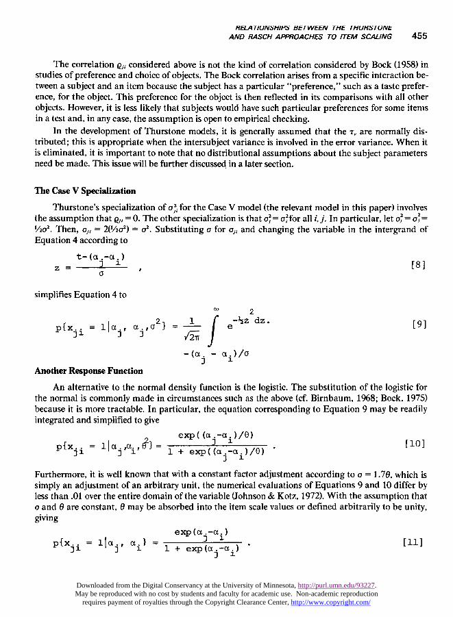
The correlation e,, considered above is not the kind of correlation considered by Bock (1958) instudies of preference and choice of objects. The Bock correlation arises from a specific interaction be-tween a subject and an item because the subject has a particular &dquo;preference,&dquo; such as a taste prefer-ence, for the object. This preference for the object is then reflected in its comparisons with all otherobjects. However, it is less likely that subjects would have such particular preferences for some itemsin a test and, in any case, the assumption is open to empirical checking.

In the development of Thurstone models, it is generally assumed that the Tv are normally dis-tributed ; this is appropriate when the intersubject variance is involved in the error variance. When itis eliminated, it is important to note that no distributional assumptions about the subject parametersneed be made. This issue will be further discussed in a later section.

The Case V Specialization

Thurstone’s specialization of 0;, for the Case V model (the relevant model in this paper) involvesthe assumption that e,, = 0. The other specialization is that o~= o,2for all i, j. In particular, let 0; = o~=1/202 . Then, o,, = 2(1/Za2) = 02. Substituting o for o,, and changing the variable in the intergrand ofEquation 4 according to

simplifies Equation 4 to

Another Response Function

An alternative to the normal density function is the logistic. The substitution of the logistic forthe normal is commonly made in circumstances such as the above (cf. Birnbaum, 1968; Bock, 1975)because it is more tractable. In particular, the equation corresponding to Equation 9 may be readilyintegrated and simplified to give

Furthermore, it is well known that with a constant factor adjustment according to o = 1.76, which issimply an adjustment of an arbitrary unit, the numerical evaluations of Equations 9 and 10 differ byless than .01 over the entire domain of the variable (Johnson & Kotz, 1972). With the assumption thato and 0 are constant, 0 may be absorbed into the item scale values or defined arbitrarily to be unity,giving



456

Bradley and Terry (1952) and Luce (1959) proposed the logistic model in Equation 11 for pairedcomparison data without reference to discriminal processes, as formulated by Thurstone.

The response functions Equations 9 and 10 have the property that the relative scale values of anypair of items of a set are invariant with respect to the values of the other items. This is an importantproperty of the models because a given collection of items need not always be kept together for the re-sulting estimates of scale values to be compatible.To summarize the development so far, one major point has shown that if the subject parameter is

introduced, as in Equation 5, then it is eliminated in the paired comparison design with the conse-quence that (1) a rationale for the assumption that e,, = 0 is provided and (2) no distributional as-sumptions need be made regarding the subjects. A second point was to draw attention to the develop-ment of Equation 10, an equation conceptually and numerically equivalent to Equation 9, which re-flects Thurstone’s Case V assumptions. Finally, it was noted that if the models of Equations 9 and 10hold, the relative scale values of a given pair of items are independent of the scale values of otheritems with which they may be scaled.

The Latent Trait Formulation

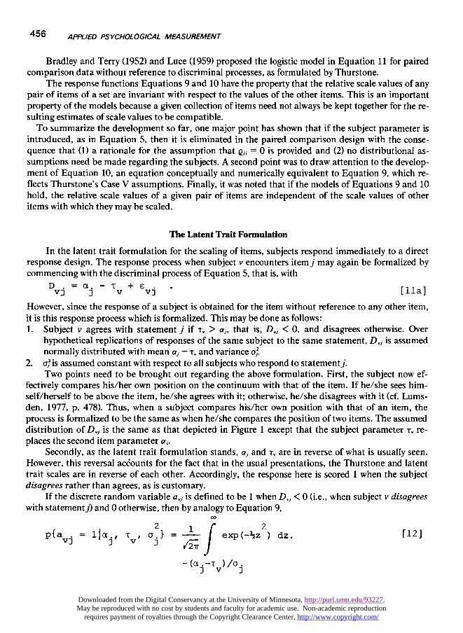
In the latent trait formulation for the scaling of items, subjects respond immediately to a directresponse design. The response process when subject v encounters itemj may again be formalized bycommencing with the discriminal process of Equation 5, that is, with

However, since the response of a subject is obtained for the item without reference to any other item,it is this response process which is formalized. This may be done as follows:1. Subject v agrees with statement j if Ty > a,, that is, D~, < 0, and disagrees otherwise. Over

hypothetical replications of responses of the same subject to the same statement, D~, is assumednormally distributed with mean a, - T, and variance 0:’

2. o; is assumed constant with respect to all subjects who respond to statement j.Two points need to be brought out regarding the above formulation. First, the subject now ef-

fectively compares his/her own position on the continuum with that of the item. If he/she sees him-self/herself to be above the item, he/she agrees with it; otherwise, he/she disagrees with it (cf. Lums-den, 1977, p. 478). Thus, when a subject compares his/her own position with that of an item, theprocess is formalized to be the same as when he/she compares the position of two items. The assumeddistribution of D~, is the same as that depicted in Figure 1 except that the subject parameter T. re-places the second item parameter a,.

Secondly, as the latent trait formulation stands, a, and T~ are in reverse of what is usually seen.However, this reversal accounts for the fact that in the usual presentations, the Thurstone and latenttrait scales are in reverse of each other. Accordingly, the response here is scored 1 when the subjectdisagrees rather than agrees, as is customary.

If the discrete random variable ay, is defined to be 1 when DVJ < 0 (i.e., when subject v disagreeswith statement j) and 0 otherwise, then by analogy to Equation 9,



457

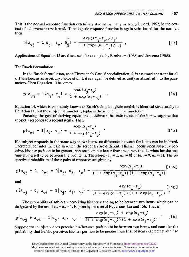
This is the normal response function extensively studied by many writers (cf. Lord, 1952, in the con-text of achievement test items). If the logistic response function is again substituted for the normal,then

Applications of Equation 13 are discussed, for example, by Birnbaum (1968) and Jensema (1968).

The Rasch Formulation

In the Rasch formulation, as in Thurstone’s Case V specialization, 9, is assumed constant for allj. Therefore, as an arbitrary choice of unit, it can again be defined as unity or absorbed into the para-meters. Then Equation 13 becomes

Equation 14, which is commonly known as Rasch’s simple logistic model, is identical structurally toEquation 11, but the subject parameter T~ replaces the second item parameter a,.

Pursuing the goal of deriving equations to estimate the scale values of the items, suppose thatsubject v responds to a second item i. Then

If a subject responds in the same way to two items, no difference between the items can be inferred.Therefore, consider the case in which the responses are different. This will occur when subject v per-ceives his/her position to be greater than one item but lesser than the other, that is, when he/she seeshimself/herself to be between the two items. Therefore, {a~, = 1, av, = 0} or {a~, = 0, av, = 1 }. The re-spective probabilities of these pairs of responses are given by

and

The probability of subject v perceiving his/her standing to be between two items, which can bedesignated by the result a, + a,, = 1, is given by the sum of Equations 15a and 15b. That is,

Suppose that subject v does perceive his/her own position to be between two items, and consider theprobability that he/she perceives his/her position to be greater than that of item i (agreeing with i so



458

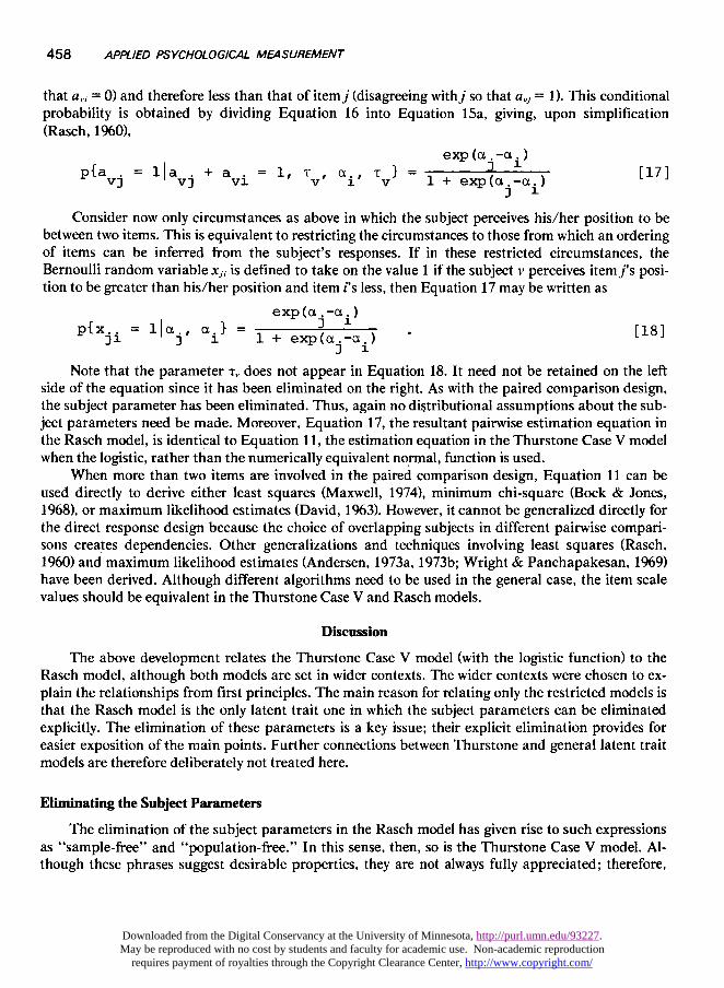
that a~, = 0) and therefore less than that of itemj (disagreeing with j so that a, = 1). This conditionalprobability is obtained by dividing Equation 16 into Equation 15a, giving, upon simplification(Rasch, 1960),

Consider now only circumstances as above in which the subject perceives his/her position to bebetween two items. This is equivalent to restricting the circumstances to those from which an orderingof items can be inferred from the subject’s responses. If in these restricted circumstances, theBernoulli random variable x,, is defined to take on the value 1 if the subject v perceives item j’s posi-tion to be greater than his/her position and item i’s less, then Equation 17 may be written as

Note that the parameter Tv does not appear in Equation 18. It need not be retained on the leftside of the equation since it has been eliminated on the right. As with the paired comparison design,the subject parameter has been eliminated. Thus, again no distributional assumptions about the sub-ject parameters need be made. Moreover, Equation 17, the resultant pairwise estimation equation inthe Rasch model, is identical to Equation 11, the estimation equation in the Thurstone Case V modelwhen the logistic, rather than the numerically equivalent normal, function is used.

When more than two items are involved in the paired comparison design, Equation 11 can beused directly to derive either least squares (Maxwell, 1974), minimum chi-square (Bock & Jones,1968), or maximum likelihood estimates (David, 1963). However, it cannot be generalized directly forthe direct response design because the choice of overlapping subjects in different pairwise compari-sons creates dependencies. Other generalizations and techniques involving least squares (Rasch,1960) and maximum likelihood estimates (Andersen, 1973a, 1973b; Wright & Panchapakesan, 1969)have been derived. Although different algorithms need to be used in the general case, the item scalevalues should be equivalent in the Thurstone Case V and Rasch models.

Discussion

The above development relates the Thurstone Case V model (with the logistic function) to theRasch model, although both models are set in wider contexts. The wider contexts were chosen to ex-plain the relationships from first principles. The main reason for relating only the restricted models isthat the Rasch model is the only latent trait one in which the subject parameters can be eliminatedexplicitly. The elimination of these parameters is a key issue; their explicit elimination provides foreasier exposition of the main points. Further connections between Thurstone and general latent traitmodels are therefore deliberately not treated here.

Eliminating the Subject Parameters

The elimination of the subject parameters in the Rasch model has given rise to such expressionsas &dquo;sample-free&dquo; and &dquo;population-free.&dquo; In this sense, then, so is the Thurstone Case V model. Al-though these phrases suggest desirable properties, they are not always fully appreciated; therefore,



459

these terms have been avoided so far. A clarification seems in order and possible in this context.Because subject parameters are eliminated explicitly, their values (individually or collectively)

need not be known. As a result, no assumptions need be made about the distribution of these para-meters in the population, for example, that they are normally distributed. This does not mean, ofcourse, that the &dquo;empirical&dquo; subject population need not be specified or described or that the scalevalues will be the same in different empirical populations. In fact, it is generally vital that the empiri-cal populations be described. But because it does not matter what the actual values of the subjectparameters are in the population, the models are, in the statistical distribution sense of population,&dquo;population-free.&dquo; This is a property of the model and independent of empirical data.

It is important to note that this holds only with respect to the estimation of the relative scalevalues of the items. It does not matter if the subject parameters are large, small, or otherwise; the sub-jects’ impressions of the relative positions of the items should be the same. That is, items whichappear more intense to one group should appear similarly more intense to the other groups. Conse-quently, different samples, whether drawn randomly or otherwise from the same empirical popula-tion, should give the same relative scale value estimates. In this sense the models are also &dquo;sample-free.&dquo;

However, this property of the model is true in empirical data only if the model holds in the data.Therefore, &dquo;sample-freeness&dquo; is always only a hypothesis until checked, as is the assumption that themodel holds. Conversely, if the relative scale values are not sample-free, the model does not holdacross these samples. This feature is often used in checks on the Rasch model, and the usual sampleformation is according to total scores on the items. Therefore, the check is with respect to an interac-tion between relative scale values and the level of the subject parameters. This is one of the bestchecks since it is then known that the subject parameter values are different. However, other samplesmay also be formed (e.g., on the basis of sex); then the check is with respect to a sex by relative scalevalue interaction. If there is no interaction, then it can be inferred that the items are working in thesame relative way in both groups. As a result, generalizability of the scale across the groups is demon-strated.

Note that it would be missing a crucial point to choose two random samples from which to check&dquo;sample-freeness&dquo; and that it would not be putting the models to any special test. Two random sam-ples should give the same relative scale values because it is an inherent assumption of all statisticalmodels that parameter estimates are &dquo;random sample-free.&dquo; For the greatest benefits, the samplesshould be systematically different.

There are two further important issues related to &dquo;sample-freeness&dquo; which need to be stressed.First, as implied above, such a property does not preclude actual differences in subject parameters.To give a concrete example, two sets of vocabulary items may have equivalent relative scale valueswith respect to groups of males and females, yet the female scores may be higher on the average thanthe male scores. However, such differences are essentially meaningful only if the relative scale valuesare equivalent in the two groups because then it is known that the items are working in the same wayin the two groups. It follows, therefore, that in comparing the mean scores of two or more groups on aset of items, one should first check that the items are working in the same way across groups.

Second, the relative scale values obtained from a sample do reflect a property of that sample,namely its impressions of the relative standing of the items. In fact, this is the sense in which Thur-stone described the samples and the empirical populations from which the samples were drawn. Hedid not concern himself with individual measurements of subjects as such. This perspective requiresno change in the models, and the perspective can be employed with the Rasch model. If two samples



460

do not give the same relative scale values for the items, then the differences between the scale valuesdescribe differences between the samples. In comparing samples, such differences in relative scalevalues may be just as informative as when no differences are found.

The Wainer, Fairbank, and Hough (WFH; 1978) StudyThe WFH study provides some data relevant to the equivalence of paired comparison and direct

response methods. One stage of this study involved subjects from four distinct empirical communitypopulations responding directly to a set of items describing events which require change in one’s life.Fifty-one items which conformed to the Rasch model within each group and which had equivalentrelative scale values across the different groups were obtained. Thus, for these respective groups, thesubject parameters did not affect the relative scale values of the items; and the items worked in thesame way across all groups. Furthermore, the relative scale value of any pair of items was not affectedby the scale values of the other items.

WFH took advantage of this latter characteristic, selecting 5 items from the 51 and submittingthem to 2 student groups of subjects in a paired comparison design. For each of these two groups, thescale values from the paired comparison data and the direct response data were equivalent after anadjustment for origin and unit. WHF were then able to adjust the remaining 46 items to the samemetric. The origin and unit were different with respect to the two student groups, but these dif-ferences were taken to characterize differences between the groups. These results indicate, however,that the relative item scale values were not affected by the subject parameters in the paired compari-son design.

WFH go on to say, &dquo;The advisability of using student samples to supplement a community sam-ple may be questioned, since there are obvious status and age differences between the two. This pro-cedure was justified by the fact that the scale ... contained only items that scaled similarly across allthe members of the community sample...&dquo; (p. 321).The items &dquo;scaled similarly&dquo; in the differentcommunity samples because the subject parameters were successfully eliminated through the Raschmodel. But what is also critical is that the subject parameters in the different student samples werealso successfully eliminated by the paired comparison design. In this connection, the WFH studyshows that their 51 items are seen to have the same relative impacts by all the empirical populationsthey investigated (whether through the paired comparison or direct response designs) and that it doesnot matter what the actual subject measures were in these populations. To the degree that their popu-lations are systematically different, the scale is generalizable; and the greater the difference in popu-lations on demographic characteristics, the greater the generalizability demonstrated.

Conclusions

In the first chapter of their book, in a section headed &dquo;Thurstone Measurement,&dquo; Bock andJones (1968, p. 9) wrote the following:

It is a mark of the maturity of a science that the number of parameters with which it dealsis small and the number of models large. In such a science, measurement can reach a high levelof perfection because, first, there is generally more than one distinct model which can be said toestimate a given parametric value. This provides the possibility for independent measurementby different methods, which serves to confirm the validity of each. Second, the science may in-clude models which make it possible to predict the effect of altered experimental conditions onthe measurement procedure.



461

This paper, and the empirical Wainer et al. study, indicate extensions in psychological scaling ofthe kind indicated by Bock and Jones. Two different experimental methods, the paired comparisonand the direct response, are shown to provide equivalent values of parameters specified in the respec-tive models. Furthermore, in the replications of the experiments in the empirical study, the contextvaried with respect to both items and subjects, but the relative scale estimates of the specified itemswas invariant. Bock and Jones go on to say, &dquo;The subjects may, and usually will, be different, and thestimuli may be different. We control the variation from individual differences among subjects merelyby insisting that subjects be sampled randomly from a specified population.&dquo; This paper also shows,therefore, that even the requirement of random sampling of subjects from a population is not only un-necessarily restrictive, but with respect to some issues, not as useful as systematic sampling.

The intention of this paper was to synthesize the models used in the WFH study and to help ex-plain some aspects of its success. That study seems critical and exemplary in the development of psy-chological measurement; and it is hoped that this paper will help other researchers to adapt theirmeasurement designs, where possible, into that framework.

References

Andersen, E.B. The numerical solution of a set ofconditional estimation equations. The Journal ofthe Royal Statistical Society, Series B, 1972, 34,42-54.

Andersen, E.B. Conditional inference for multiplechoice questionnaires. British Journal of Mathe-matical and Statistical Psychology, 1973, 26,31-44. (a)

Andersen, E.B. A goodness of fit test for the Raschmodel. Psychometrika, 1973, 38, 123-140. (b)

Birnbaum, A. Some latent trait models and their usein inferring an examinee’s ability. In F.M. Lord &M.R. Novick, Statistical theories of mental testscores. Reading, MA: Addison-Wesley, 1968.

Bock, R.D. Remarks on the test of significance forpaired comparisons. Psychometrika, 1958, 23,323-334.

Bock, R.D. Multivariate statistical methods inbehavioral research. New York: McGraw-Hill,1975.

Bock, R.D., & Jones, L.V. The measurement and pre-diction of judgement and choice. San Francisco:Holden-Day, 1968.

Bradley, R.A., & Terry, M.E. Rank analysis of in-complete block designs. I. The method of pairedcomparisons. Biometrika, 1952, 39, 324-345.

David, H.A. The method of paired comparisons. NewYork: Hafner, 1963.

Edwards, A. L. Techniques of attitude scale construc-tion. New York: Appleton-Century-Crofts, 1957.

Jensema, C.J. An application of latent trait mentaltest theory. British Journal of Mathematical andStatistical Psychology, 1974, 27, 29-48.

Johnson, N.L., & Kotz, S. Distributions in statistics:Continuous univariate distributions (Vol. 3). NewYork: Wiley, 1972.

Lord, F.M. A theory of test scores. PsychometricMonograph No. 7, 1952.

Luce, R.D. Individual choice behavior. New York:Wiley, 1959.

Lumsden, J. Person reliability. Applied PsychologicalMeasurement, 1977, 1, 477-482.

Maxwell, A.E. The logistic transformation in the

analysis of paired-comparison data. British Jour-nal of Mathematical and Statistical Psychology,1974, 27, 62-71.

Rasch, G. Probabilistic models for some intelligenceand attainment tests. Copenhagen: Danish Insti-tute for Educational Research, 1960.

Rasch, G. On general laws and the meaning of meas-urement in psychology. Proceedings of the FourthBerkeley Symposium on Mathematical Statistics,1961, 4, 321-334.

Thurstone, L.L. A law of comparative judgement.Psychological Review, 1927, 34, 278-286. (a)

Thurstone, L.L. The method of paired comparisonsfor social values. Journal of Abnormal Social Psy-chology, 1927, 21, 384-400. (b)

Thurstone, L.L. Psychophysical analysis. AmericanJournal of Psychology, 1927, 38, 368-389. (c)

Thurstone, L.L. The measurement of opinion. Jour-nal of Abnormal Social Psychology, 1928, 22,415-430.

Torgerson, W.S. Theory and methods of scaling. NewYork: John Wiley, 1958.

Wainer, H., Fairbank, D.T., & Hough, R.L. Predict-ing the impact of simple and compound life

change events. Applied Psychological Measure-ment, 1978, 2, 313-322.

Wright, B.D. Sample-free test calibration and personmeasurement. Proceedings of the 1967 Invita-tional Conference on Testing Problems. Prince-ton, NJ: Educational Testing Service 1967,85-101.



462

Wright, B.D., & Panchapakesan, N. A procedure forsample-free item analysis. Educational and Psy-chological Measurement, 1969, 29, 23-48.

Wright, B.D., & Douglas, G.A. Best procedures forsample-free item analysis. Applied PsychologicalMeasurement, 1977, 1, 281-295.

Author’s Address

David Andrich, Department of Education, The Uni-versity of Western Australia, Nedlands, Western,Australia, 6009.



Documents

Approaches to Item Scaling - Conservancy - University of Minnesota