Approximation schemes for job shop scheduling problems with controllable processing times

European Journal of Operational Research 167 (2005) 297–319

www.elsevier.com/locate/dsw

Discrete Optimization

Approximation schemes for job shop scheduling problemswith controllable processing times q

Klaus Jansen a, Monaldo Mastrolilli b,*, Roberto Solis-Oba c

a Universit€at zu Kiel, Christian-Albrechts Platz 4, D-24198 Kiel, Germanyb IDSIA––Istituto Dalle Molle di Studi sull’ Intelligenza Artificiale, Galleria 2, Manno 6928 Lugano, Switzerland

c Department of Computer Science, The University of Western Ontario, London, ON, N6A 5B7 Canada

Received 22 March 2002; accepted 31 March 2004

Available online 20 June 2004

Abstract

In this paper we study the job shop scheduling problem under the assumption that the jobs have controllable

processing times. The fact that the jobs have controllable processing times means that it is possible to reduce the

processing time of the jobs by paying a certain cost. We consider two models of controllable processing times:

continuous and discrete. For both models we present polynomial time approximation schemes when the number of

machines and the number of operations per job are fixed.

� 2004 Elsevier B.V. All rights reserved.

Keywords: Scheduling; Job shop; Controllable processing times; Approximation schemes

1. Introduction

Most scheduling models assume that jobs have fixed processing times. However, in real-life applications

the processing time of a job often depends on the amount of resources such as facilities, manpower, funds,

etc. allocated to it, and so its processing time can be reduced when additional resources are assigned to thejob. A scheduling problem in which the processing times of the jobs can be reduced at some expense is

called a scheduling problem with controllable processing times. Scheduling problems with controllable

processing times have gained importance in scheduling research since the pioneering works of Vickson

[23,24]. For a survey of this area until 1990, the reader is referred to [17]. Recent results include [2–

4,10,14,15,20,22,26].

qA preliminary version of this paper appeared in the Seventh Italian Conference on Theoretical Computer Science (ICTCS’01).* Corresponding author. Tel.: +41-91-610-86-64; fax: +41-91-610-86-61.

E-mail addresses: [email protected] (K. Jansen), [email protected] (M. Mastrolilli), [email protected] (R. Solis-Oba).

0377-2217/$ - see front matter � 2004 Elsevier B.V. All rights reserved.

doi:10.1016/j.ejor.2004.03.025

mailto:[email protected]

298 K. Jansen et al. / European Journal of Operational Research 167 (2005) 297–319

1.1. Job shop scheduling with controllable processing times

The job shop scheduling problem is a fundamental problem in Operations Research. In this problem

there is a set J ¼ fJ1; . . . ; Jng of jobs that must be processed by a group of m machines. Every job Jjconsists of an ordered sequence of at most l operations O1j;O2j; . . . ;Okjj, kj 6 l. For every operation Oij

there is a specific machine mij that must process it during pij units of time. A machine can process only one

operation at a time, and for any job at most one of its operations can be processed at any moment.

The problem is to schedule the jobs so that the maximum completion time Cmax is minimized. Time Cmax iscalled the length or makespan of the schedule.

In the non-preemptive version of the job shop scheduling problem, operations must be processed without

interruption. The preemptive version allows an operation to be interrupted and continued at a later time. In

the job shop scheduling problem with controllable processing times a feasible solution is specified by a

schedule r that indicates the starting times for the operations and a vector d that gives their processing

times and costs. Let us denote by T ðr; dÞ the makespan of schedule r with processing times according to d,and let CðdÞ be the total cost of d. We define, and study, the following three optimization problems.

P1. Minimize T ðr; dÞ, subject to CðdÞ6j, for some given value j > 0.

P2. Minimize CðdÞ, while ensuring that T ðr; dÞ6 s, for some given value s > 0.

P3. Minimize T ðr; dÞ þ aCðdÞ, for some given value a > 0.

We consider two variants of each one of the three above problems. The first variant allows continuous

changes to the processing times of the operations. In this case, we assume that the cost of reducing the

processing time of an operation is an affine function of the processing time. This is a common assumption

made when studying problems with controllable processing times [20,22]. The second variant allows onlydiscrete changes to the processing times of the operations, and there is a finite set of possible processing

times and costs for every operation Oij.

1.2. Known results

The job shop scheduling problem is considered to be one of the most difficult to solve problems in

combinatorial optimization, both, from the theoretical and the practical points of view. The problem is NP-

hard even if each job has at most three operations, there are only two machines, and processing times arefixed [8]. The job shop scheduling problem is also NP-hard if there are only 3 jobs and 3 machines [21].

Moreover, the problem is NP-hard in the strong sense if each job has at most three operations and there are

only three machines [6]. The same result holds if preemptive schedules are allowed [8]. The problems ad-

dressed in this paper are all generalizations of the job shop scheduling problem with fixed processing times,

and therefore, they are strongly NP-hard. Moreover, Nowicki and Zdrzalka [16] show that the version

of problem P3 for the less general flow shop problem with continuously controllable processing times is

NP-hard even when there are only two machines.

The practical importance of NP-hard problems necessitates efficient ways of dealing with them. A veryfruitful approach has been to relax the notion of optimality and settle for near-optimal solutions. A near-

optimal solution is one whose objective function value is within some small multiplicative factor of the

optimal. Approximation algorithms are heuristics that in polynomial time provide provably near-optimal

solutions. A polynomial time approximation scheme (PTAS for short) is an approximation algorithm which

produces solutions of value within a factor ð1þ eÞ of the optimum, for any value e > 0.

Williamson et al. [25] proved that the non-preemptive job shop scheduling problem does not have a

polynomial time approximation algorithm with worst case bound smaller than 54unless P ¼ NP. The best

known approximation algorithm [7] has worst case bound OððlogðmlÞ logðminðml; pmaxÞÞ=log logðmlÞÞ2Þ,

K. Jansen et al. / European Journal of Operational Research 167 (2005) 297–319 299

where pmax is the largest processing time among all operations. For those instances where m and l are fixed(the restricted case we are focusing on in this paper), Shmoys et al. [19] gave a ð2þ eÞ-approximation

algorithm for any fixed e > 0. This result has recently been improved by Jansen et al. [5,12] who designed a

PTAS that runs in linear time. On the other hand the preemptive version of the job shop scheduling

problem is NP-complete in the strong sense even when m ¼ 3 and l ¼ 3 [8]. When processing times are

controllable, to the best of our knowledge, the only known closely related result is due to Nowicki [15]. In

[15] the flow shop scheduling problem with controllable processing times is addressed, and a 4/3-approx-

imation algorithm for the flow shop version of problem P3 is described.

1.3. New results

We present the first known polynomial time approximation schemes for problems P1, P2, and P3, when

the number m of machines and the number l of operations per job are fixed.

For problem P1 we present an algorithm which finds a solution ðr; dÞ of cost at most j and makespan no

larger than ð1þ OðeÞÞ times the optimum makespan, for any given value e > 0. We observe that, since for

problem P2 deciding whether there is a solution of length T ðr; dÞ6 s is already NP-complete, then unless

P¼NP, we might only expect to obtain a solution with cost at most the optimal cost and makespan notgreater than sð1þ eÞ, for a given value e > 0. Our algorithm for problem P3 finds a solution of value at

most ð1þ OðeÞÞ times the optimum, for any e > 0.

Our algorithms can handle both, continuously and discretely controllable processing times, and they can

be extended to the case of convex piecewise linear cost functions. Our algorithms have a worst case per-

formance ratio that is better than the 4/3-approximation algorithm for problem P3 described in Nowicki

[15]. Moreover, the linear time complexity of our PTAS for problem P3 is the best possible with respect to

the number of jobs.

Our algorithms are based on a paradigm that has been successfully applied to solve other schedulingproblems. First, partition the set of jobs into ‘‘large’’, ‘‘medium’’ and ‘‘small’’ jobs. The sets of large and

medium jobs have a constant number of jobs each. We compute all possible schedules for the large jobs.

Then, for each one of them, schedule the remaining jobs inside the empty gaps that the large jobs leave by

first using a linear program to assign jobs to gaps, and then computing a feasible schedule for the jobs

assigned to each gap.

A major difficulty with using this approach for our problems is that the processing times and costs of the

operations are not fixed, so we must determine these values before we can use the above approach. One

possibility is to use a linear program to assign jobs to gaps and to determine the processing times and costsof the operations. But, we must be careful since, for example, a natural extension of the linear program

described in [12] defines a polytope with an exponential number of extreme points, and it does not seem to

be possible to solve such linear program in polynomial time. We show how to construct a small polytope

with only a polynomial number of extreme points that contains all the optimum solutions of the above

linear program. This polytope is defined by a linear program that can be solved exactly in polynomial time

and approximately, to within any pre-specified precision, in fully polynomial time (i.e. polynomial also in

the multiplicative inverse of the precision).

Our approach is general enough that it can be used to design polynomial time approximation schemesfor both the discrete and the continuous versions of problems P1–P3 with and without preemptions. In this

paper we present polynomial time approximation schemes for the continuous version of problems P1–P3,

and a PTAS for the discrete version of P3. The polynomial time approximation schemes for the discrete

version of P1 and P2 can be easily derived from the results described here. We present a series of trans-

formations that simplify any instance of the above problems. Some transformations may potentially in-

crease the value of the objective function by a factor of 1þ OðeÞ, for a given value e > 0, so we can perform

a constant number of them while still staying within 1þ OðeÞ of the optimum. We say that this kind of


transformations produce 1þ OðeÞ loss. A transformation that does not modify the value of the optimumsolution is said to produce no loss. In the following, for simplicity of notation, we assume that 1=e is anintegral value.

1.4. Organization

The rest of the paper is organized in the following way. We first address problems with continuous

processing times. In Sections 2 and 3, we present polynomial time approximation schemes for problem P1

with and without preemptions. In Sections 4 and 5 we present polynomial time approximation schemes forproblems P2 and P3. In Section 6 we study problem P3 with discrete processing times, and show how to

design a linear time PTAS for it.

2. Non-preemptive problem P1 with continuous processing times

Problem P1 is to compute a schedule with minimum makespan and cost at most j for some given value

j. In the case of continuously controllable processing times, we assume that for each operation Oij there isan interval ½‘ij; uij�, 06 ‘ij 6 uij, specifying its possible processing times. The cost for processing an operation

Oij in time ‘ij is denoted as c‘ij P 0 and for processing it in time uij the cost is cuij P 0. For any value dij 2 ½0; 1�the cost for processing operation Oij in time

pdijij ¼ dij‘ij þ ð1� dijÞuij
is
cdijij ¼ dijc‘ij þ ð1� dijÞcuij:

We assume that ‘ij, uij, c‘ij, cuij and dij are rational numbers. Moreover, without loss of generality, we

assume that for every operation Oij, cuij 6 c‘ij, and if cuij ¼ c‘ij then uij ¼ ‘ij.

Remark 1. For simplicity, we assume that the total cost of any solution is at most 1. To see why, let usconsider an instance of problem P1. Divide all cuij and c‘ij values by j to get an equivalent instance in which

the bound on the total cost of the solution is 1, i.e.

CðdÞ ¼Xn

j¼1

Xl

i¼1cdijij 6 1:

Moreover, since the total cost is at most 1, without loss of generality we can assume that the maximum

cost for each operation is at most 1. More precisely, if c‘ij > 1 for some operation Oij, we set c‘ij ¼ 1 and

make

‘ij ¼uijðc‘ij � 1Þ � ‘ijðcuij � 1Þ

c‘ij � cuij

to get an equivalent instance of the problem in which c‘ij 6 1 for all operations Oij.

2.1. Lower and upper bounds for the problem

In the following we compute lower (LB) and upper (UB) bounds for the optimum makespan. Let

U ¼Pn

j¼1Pl

i¼1 uij. Consider an optimal solution ðr�; d�Þ for problem P1 and let us use OPT to denote the

optimum makespan. Let P � ¼Pn

j¼1Pl

i¼1 pd�ijij ¼

Pnj¼1

Pli¼1 ð‘ij � uijÞd�ij þ U be the sum of the processing


times of all jobs in this optimum solution. Define cij ¼ c‘ij � cuij, so Cðd�Þ ¼Pn

j¼1Pl

i¼1 ðcijd�ij þ cuijÞ6 1. Note

that d� is a feasible solution for the following linear program.

min P ¼Xn

j¼1

Xl

i¼1ð‘ij � uijÞxij þ U

s:t:Xn

j¼1

Xl

i¼1xijcij 6 1�

Xn

j¼1

Xl

i¼1cuij;

06 xij 6 1 8j ¼ 1; . . . ; n and i ¼ 1; . . . ; l:

Let ~x be an optimal solution for this linear program and let P ð~xÞ be its value. Observe that Pð~xÞ6 P � andCð~xÞ6 1. Moreover, note that

• if 1�Pn

j¼1Pl

i¼1 cuij < 0, then there exists no solution with cost at most 1.

• If 1�Pn

j¼1Pl

i¼1 cuij ¼ 0 then in any feasible solution with cost at most 1, the processing time of each

operation Oij must be uij. In this case we know that U=m6OPT6U , since the total sum of the process-

ing times of all the operations is U . By dividing all processing times by U , we get the bounds

LB ¼ 1=m6OPT6UB ¼ 1.

• If 1�Pn

j¼1Pl

i¼1 cuij > 0, we simplify the instance by dividing all costs by 1�

Pnj¼1

Pli¼1 c

uij. Then, the

above linear program can be simplified as follows:

maxXn

j¼1

Xl

i¼1tijxij

s:t:Xn

j¼1

Xl

i¼1xijwij 6 1;

06 xij 6 1 j ¼ 1; . . . ; n and i ¼ 1; . . . ; l;

where tij ¼ uij � ‘ij and wij ¼ cij=ð1�Pn

j¼1Pl

i¼1 cuijÞ.

This linear program is a relaxation of the classical knapsack problem, which can be solved as follows

[13]. Sort the operations in non-increasing order of ratio value tij=wij. Consider, one by one, the operations

Oij in this order, assigning to each one of them value xij ¼ 1 as long as their total weightPn

j¼1Pl

i¼1 xijwij is

at most 1. If necessary, assign to the next operation a fractional value to ensure that the total weight of the

operations is exactly 1. Set xij ¼ 0 for all the remaining operations. This algorithm runs in OðnlÞ time [13].

If we schedule all the jobs one after another with processing times as defined by the optimal solution ~x of theknapsack problem, we obtain a feasible schedule for the jobs J with makespan P ð~xÞ. Since

P ð~xÞP P �POPTP P �=mP Pð~xÞ=m, then by dividing all ‘ij and uij values by P ð~xÞ, we get the same boundsas above, i.e., LB ¼ 1=m and UB¼ 1.

2.2. Overview of the algorithm

We might assume without loss of generality that each job has exactly l operations. To see this, consider a

job Ji with li < l operations O1i;O2i; . . .Oli i. We create l� li new operations Oij with zero processing time

and cost, i.e., we set ‘ij ¼ uij ¼ 0 and cuij ¼ c‘ij ¼ 0. Each one of these operations must be processed in the

same machine which must process operation Olii. Clearly, the addition of these operations does not changethe makespan of any feasible schedule for J.

We briefly sketch the algorithm here and give the details in the following sections. Let j > 0 be the upper

bound on the cost of the solution and e > 0 be a positive value. Consider an optimum solution ðr�; d�Þ for


the problem; let s� be the makespan of this optimum solution. Our algorithm finds a solution ðr; dÞ of costCðdÞ6 j and makespan at most ð1þ OðeÞÞs�.

1. Partition the jobs into 3 groups: L (large), M (medium), and S (small). Set L contains the largest

k6m2=e jobs according to the optimum solution ðr�; d�Þ. Set M contains the qlm2=e� 1 next largest

jobs, where q ¼ 6l4m3=e. The value for k is chosen so that the total processing time of the medium jobs

in solution ðr�; d�Þ is at most es� (the exact value for k is given in Section 2.6). The set S of small jobs is

formed by the remaining jobs. Note that jLj and jMj are constant. It is somewhat surprising to know

that we can determine the sets L;M, and S, even when an optimum solution ðr�; d�Þ is not known. Weshow in Section 2.6 how to do this. From now on we assume that we know sets L, M, and S. An oper-

ation that belongs to a large, medium, or small job is called a large, medium, or small operation, respec-

tively, regardless of its processing time.

2. Determine the processing times and costs for the medium operations.

3. Try all possible ways of scheduling the large jobs on the machines. Each feasible schedule for L leaves a

set of empty gaps where the small and medium jobs can be placed. For each feasible schedule for the

large jobs use a linear program to determine the processing times and costs for the small and large oper-

ations, and to determine the gaps where each small and medium operation must be scheduled. then,transform this assignment into a feasible schedule for the entire set of jobs.

4. Output the schedule with minimum length found in Step 3.

2.3. Simplifying the input

We can simplify the input by reducing the number of possible processing times for the operations. We

begin by showing that it is possible to upper bound the processing times of small operations by eqklm.

Lemma 2. With no loss, for each small operation Oij we can set uij �uij and cuij c‘ij�c

uij

uij�‘ij ðuij � �uijÞ þ cuij, where�uij ¼ minfuij; e

qklmg.

Proof. As it was shown in Section 2.1, the optimal makespan is at most 1 and, therefore, the sum of the

processing times of all jobs cannot be larger than m. Let P �j ¼Pl

i¼1 pd�ijij be the sum of the processing times of

the operations of job Jj according to an optimum solution ðr�; d�Þ. Let p be the length of the longest small

job according to this optimum solution. By definition of L and M,

jL [Mj � p ¼ klm2qe

p6X

Jj2M[LP �j 6m;

and so p6 eqklm. Hence, the length of an optimum schedule is not increased if the largest processing time uij

of any small operation Oij is set to �uij ¼ minfuij; eqklmg. If we do this, we also need to set cuij

c‘ij�cuij

uij�‘ij ðuij��uijÞ þ cuij (this is the cost to process operation Oij in time �uij). h

In order to compute a 1þ OðeÞ-approximate solution for P1 we show that it is sufficient to consider only

a constant number of different processing times and costs for the medium jobs.

Lemma 3. There exists a ð1þ 2eÞ-optimal schedule where each medium operation has processing time of theform e

mjMjl ð1þ eÞi, for i 2 N.


Proof. Let A be the set of medium operations for which pd�ijij 6

emjMjl. Since cuij 6 c‘ij, by increasing the pro-

cessing time of any operation, its corresponding cost cannot increase. Therefore, if we increase the pro-

cessing times for the operations in A to emjMjl, the makespan increases by at most jAj e

mjMjl 6 e=m, and so the

length of an optimum solution would increase by at most a factor of 1þ e. For the remaining medium

operations, round up their processing times pd�ijij to the nearest value of the form e

mjMjl ð1þ eÞi, for some

i 2 N. Since this rounding increases the processing time by at most a factor 1þ e, the value of an optimum

solution increases by at most the same factor, 1þ e. h

By the discussion in Section 2.1, the processing times of the operations are at most 1. By the previous

lemma, the number of different processing times for medium operations is OðlogðmjMjlÞ=eÞ (clearly, thesame bound applies to the number of different costs). Since there is a constant number of medium oper-

ations after the above rounding, there is also a constant number of choices for the values of their processing

times and costs.

Let the rounded processing times and costs for the medium operations be denoted as �pij and �cij. Belowwe show that when the medium operations are processed according to these ð�pij;�cijÞ-values, it is possible tocompute a 1þ OðeÞ-approximate solution for problem P1 in polynomial time. Let us consider allOðlogðmjMjlÞ=eÞ possible choices for processing times for the medium operations. Clearly, for one of such

choices the processing times and costs are as described in Lemma 3. Hence, from now on, we assume that

we know these ð�pij;�cijÞ-values for the medium operations. In order to simplify the following discussion, for

each medium operation Oij we set ‘ij ¼ uij ¼ �pij and c‘ij ¼ cuij ¼ �cij, thus, fixing their processing times and

costs.

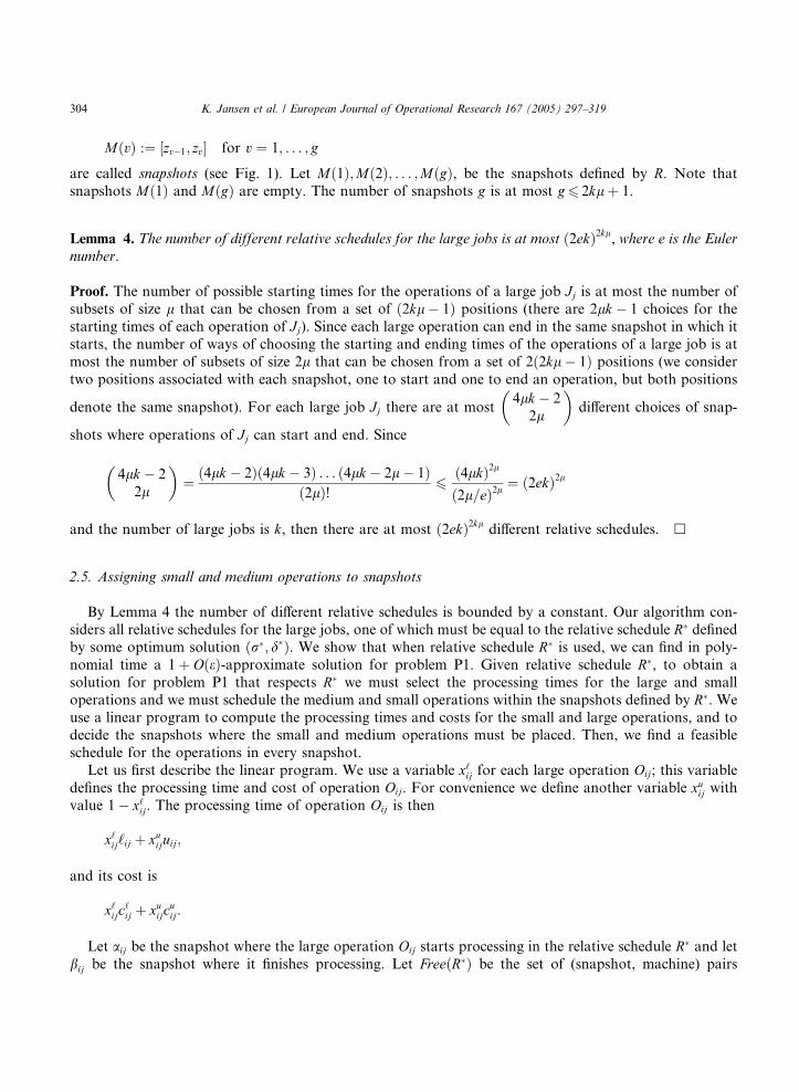
2.4. Relative schedules

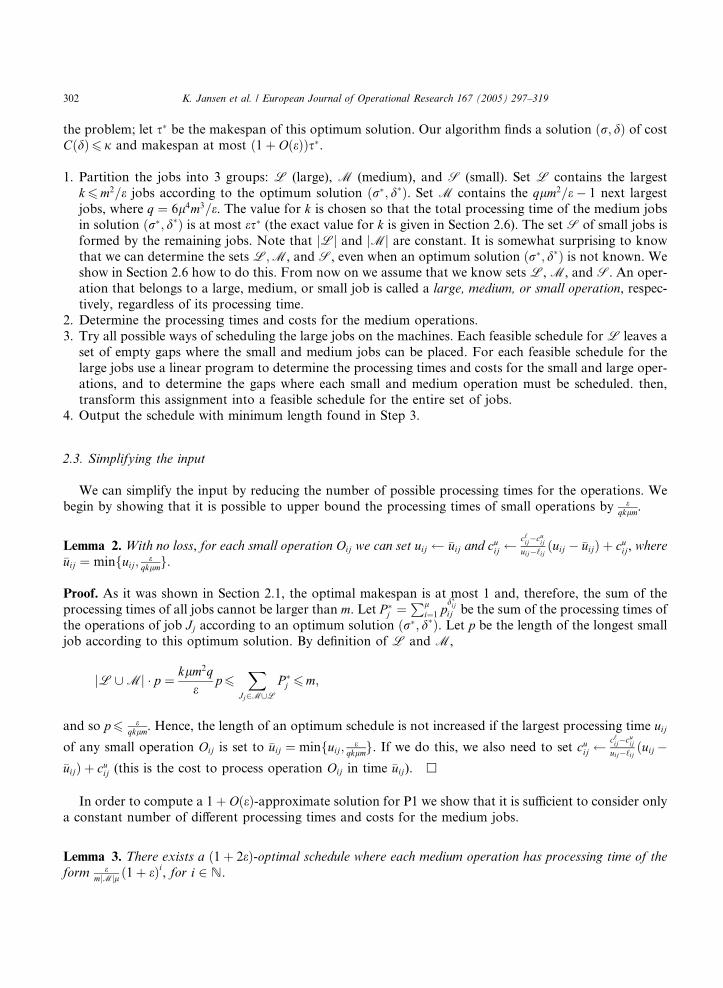
A relative schedule for the large operations is an ordering of the starting and ending times of the

operations. We say that a feasible schedule S for the large operations respects a relative schedule R if the

starting and ending times of the operations as defined by S are ordered as indicated in R (breaking ties in an

appropriate way), see Fig. 1. Fix a relative schedule R for the large operations. The starting, sij, and fin-

ishing, fij, times of an operation Oij define an interval ½sij; fij� where each operation Oij must be processed

(see Fig. 1). Let

Fig. 1

schedu

z1 < z2 < � � � < zg�1

be the ordered sequence of all different sij and fij values, for j ¼ 1; . . . ; n and i ¼ 1; . . . ; l. Let us introducetwo additional values zg P zg�1 and z0 6 z1 to bound intervals without large operations. The intervals

z0

31O22O

21O

13O

12O 3332

z2 z3 z4 z5 z6 z7 z8 z 10zz1

snapshot 2 ...snapshot 1

9

2311 O

OO

O

machine 3

machine 2

machine 1

. A feasible schedule for the set of jobs fJ1; J2; J3g, each consisting of 3 large operations, that respects the following relative

le: R ¼ ðs11; s13; s12; f11; f13; s23; f12; s21; s22; f21; f22; s32; s31; f23; f32; s33; f31; f33Þ.


MðvÞ :¼ ½zv�1; zv� for v ¼ 1; . . . ; g

are called snapshots (see Fig. 1). Let Mð1Þ;Mð2Þ; . . . ;MðgÞ, be the snapshots defined by R. Note that

snapshots Mð1Þ and MðgÞ are empty. The number of snapshots g is at most g6 2klþ 1.

Lemma 4. The number of different relative schedules for the large jobs is at most ð2ekÞ2kl, where e is the Eulernumber.

Proof. The number of possible starting times for the operations of a large job Jj is at most the number of

subsets of size l that can be chosen from a set of ð2kl� 1Þ positions (there are 2lk � 1 choices for the

starting times of each operation of Jj). Since each large operation can end in the same snapshot in which it

starts, the number of ways of choosing the starting and ending times of the operations of a large job is at

most the number of subsets of size 2l that can be chosen from a set of 2ð2kl� 1Þ positions (we consider

two positions associated with each snapshot, one to start and one to end an operation, but both positions

denote the same snapshot). For each large job Jj there are at most4lk � 2

2l

� �different choices of snap-

shots where operations of Jj can start and end. Since

4lk � 2

2l

� �¼ ð4lk � 2Þð4lk � 3Þ . . . ð4lk � 2l� 1Þ

ð2lÞ! 6ð4lkÞ2l

ð2l=eÞ2l¼ ð2ekÞ2l

and the number of large jobs is k, then there are at most ð2ekÞ2kl different relative schedules. h

2.5. Assigning small and medium operations to snapshots

By Lemma 4 the number of different relative schedules is bounded by a constant. Our algorithm con-

siders all relative schedules for the large jobs, one of which must be equal to the relative schedule R� definedby some optimum solution ðr�; d�Þ. We show that when relative schedule R� is used, we can find in poly-

nomial time a 1þ OðeÞ-approximate solution for problem P1. Given relative schedule R�, to obtain a

solution for problem P1 that respects R� we must select the processing times for the large and small

operations and we must schedule the medium and small operations within the snapshots defined by R�. We

use a linear program to compute the processing times and costs for the small and large operations, and todecide the snapshots where the small and medium operations must be placed. Then, we find a feasible

schedule for the operations in every snapshot.

Let us first describe the linear program. We use a variable x‘ij for each large operation Oij; this variable

defines the processing time and cost of operation Oij. For convenience we define another variable xuij withvalue 1� x‘ij. The processing time of operation Oij is then

x‘ij‘ij þ xuijuij;

and its cost is

x‘ijc‘ij þ xuijc

uij:

Let aij be the snapshot where the large operation Oij starts processing in the relative schedule R� and let

bij be the snapshot where it finishes processing. Let FreeðR�Þ be the set of (snapshot, machine) pairs


ðMð‘Þ; hÞ such that no large operation is scheduled by R� in snapshotMð‘Þ on machine h. For every mediumand small job Jj, let Kj be the set of tuples of the form ðs1; s2; . . . ; slÞ such that 16 s1 6 s2 6 � � � 6 sl 6 g; andðsi;mijÞ 2 FreeðR�Þ, for all i ¼ 1; . . . ; l. This set Kj determines the free snapshots where it is possible to place

the operations of job Jj.Let D ¼ fðd1; d2; . . . ; dlÞjdk 2 0; 1f g for all k ¼ 1; . . . ; lg be the set of all l-dimensional binary vectors.

For each medium and small job Jj we define a set of at most ð2gÞl variables xj;ðs;dÞ, where s 2 Kj and d 2 D.These variables will indicate the snapshots where small and medium jobs will be scheduled. To understand

the meaning of these variables, let us define

xijðw; 1Þ ¼X

ðs;dÞ2Kj�D;si¼w;di¼1xj;ðs;dÞ;

and

xijðw; 0Þ ¼X

ðs;dÞ2Kj�D;si¼w;di¼0xj;ðs;dÞ;

for each operation i, job Jj, and snapshotMðwÞ. Given a set of values for the variables xj;ðs;dÞ, they define theprocessing times for the jobs and they also give an assignment of medium and small operations to snap-

shots: the amount of time that an operation Oij is processed within snapshot MðwÞ is xijðw; 1Þ � ‘ijþxijðw; 0Þ � uij, and the fraction of Oij that is assigned to this snapshot is xijðw; 0Þ þ xijðw; 1Þ.

Example 1. Consider an instance with l ¼ 2 having a job Jj with the following processing time functions:

O1j pd1j1j ¼ 0:5 � d1j þ ð1� d1jÞ;

O2j pd2j2j ¼ 0:1 � d2j þ 0:5 � ð1� d2jÞ:

Furthermore, assume that in some feasible solution p1j ¼ 0:65 and p2j ¼ 0:34, and operation O1j is placed

on the third snapshot, while operation O2j is in the seventh snapshot. By setting xj;ðð3;7Þ;ð0;0ÞÞ ¼ 0:3,xj;ðð3;7Þ;ð0;1ÞÞ ¼ 0, xj;ðð3;7Þ;ð1;0ÞÞ ¼ 0:3 and xj;ðð3;7Þ;ð1;1ÞÞ ¼ 0:4, we see that p1j ¼ ðxj;ðð3;7Þ;ð0;0ÞÞ þ xj;ðð3;7Þ;ð0;1ÞÞÞ þðxj;ðð3;7Þ;ð1;0ÞÞ þ xj;ðð3;7Þ;ð1;1ÞÞÞ � 0:5 ¼ 0:65, and p2j¼ðxj;ðð3;7Þ;ð0;0ÞÞ þxj;ðð3;7Þ;ð1;0ÞÞÞ�0:5þðxj;ðð3;7Þ;ð0;1ÞÞ þxj;ðð3;7Þ;ð1;1ÞÞÞ�0:1 ¼ 0:34:

For each snapshot Mð‘Þ we use a variable t‘ to denote its length. For any ð‘; hÞ 2 FreeðR�Þ, we define theload L‘;h of machine h in snapshot Mð‘Þ as the total processing time of the small and medium operations

that are assigned to h in Mð‘Þ, i.e.,

L‘;h ¼X

Jj2S[M

Xl

i¼1mij¼h

xijð‘; 1Þ‘ij�

þ xijð‘; 0Þuij�: ð1Þ

The total cost of a schedule is given by

C ¼X

Jj2S[M

Xg

‘¼1

Xl

i¼1xijð‘; 1Þc‘ij

�þ xijð‘; 0Þcuij

�þ

XJj2L

Xl

i¼1x‘ijc

‘ij þ xuijc

uij

� �:

We use the following linear program LPðR�Þ to determine processing times and costs of large and smalloperations, and to allocate small and medium operations to snapshots.


min T ¼Xg

‘¼1t‘

s:t: C6 1; ðc1Þ

Xbij‘¼aij

t‘ ¼ x‘ij‘ij þ xuijuij; Jj 2L; i ¼ 1; . . . ; l; ðc2Þ

x‘ij þ xuij ¼ 1; Jj 2L; i ¼ 1; . . . ; l; ðc3ÞXðs;dÞ2Kj�D

xj;ðs;dÞ ¼ 1; Jj 2 S [M; ðc4Þ

L‘;h 6 t‘; ð‘; hÞ 2 FreeðR�Þ; ðc5Þ

x‘ij; xuij P 0; Jj 2L; i ¼ 1; . . . ; l; ðc6Þ

xj;ðs;dÞP 0; Jj 2S [M; ðs; dÞ 2 Kj � D; ðc7Þt‘ P 0; ‘ ¼ 1; . . . ; g: ðc8Þ

In this linear program the value of the objective function T is the length of the schedule, which we want to

minimize. Constraint (c1) ensures that the total cost of the solution is at most one. Condition (c2) requires

that the total length of the snapshots where a large operation is scheduled is exactly equal to the length of

the operation. Constraint (c4) assures that every small and medium operation is completely assigned to

snapshots, while constraint (c5) checks that the total load of every machine h during each snapshot ‘ doesnot exceed the length of the snapshot. Let ðr�; d�Þ denote an optimal schedule where the processing timesand costs of medium jobs are fixed as described in the previous section.

Lemma 5. The optimal solution of LPðR�Þ has value no larger than the makespan of ðr�; d�Þ.

Proof. We only need to show that ðr�; d�Þ defines a feasible solution for LPðR�Þ. For any operation Oij, let

pd�ijij ðwÞ be the amount of time that Oij is processed during snapshot MðwÞ in the optimum schedule ðr�; d�Þ.We determine now the values for the variables t�‘ ; x

‘�ij ; x

u�ij , and x�j;ðs;dÞ defined by ðr�; d�Þ. Set x‘�ij ¼ d�ij and

xu�ij ¼ 1� d�ij for all large operations Oij. The values for the variables t�‘ can be easily obtained from thesnapshots defined by the large operations. Let

x�ijðw; 1Þ ¼ d�ijpd�ijij ðwÞ

pd�ijij

;

and

x�ijðw; 0Þ ¼ ð1� d�ijÞpd�ijij ðwÞ

pd�ijij

:

The processing time pd�ijij ðwÞ and cost c

d�ijij ðwÞ of Oij can be written as x�ijðw; 1Þ‘ij þ x�ijðw; 0Þuij and

x�ijðw; 1Þc‘ij þ x�ijðw; 0Þcuij, respectively. Now we show that there is a feasible solution x�j;ðs;dÞ for LPðR�Þ suchthat

(i) x�ijðw; 1Þ ¼Pðs;dÞ2Kj�D;si¼w;di¼1 x

�j;ðs;dÞ, and

(ii) x�ijðw; 0Þ ¼Pðs;dÞ2Kj�D;si¼w;di¼0 x

�j;ðs;dÞ.


Therefore, for this solution, pd�ijij ðwÞ and c

d�ijij ðwÞ are linear combinations of the variables x�j;ðs;dÞ. We

determine the values for the variables x�j;ðs;dÞ as follows.

1. For each job Jj 2S [M do

2. Compute Sj ¼ fði;w; dÞjx�ijðw; dÞ > 0; i ¼ 1; . . . ; l;w ¼ 1; . . . ; g; d ¼ 0; 1g.3. If Sj ¼ ; then exit.

4. Let f ¼ minfx�ijðw; dÞjði;w; dÞ 2 Sjg and let I ;W , and D be such that x�IjðW ;DÞ ¼ f .5. Let s ¼ ðs1; s2; . . . ; slÞ 2 Kj and d ¼ ðd1; d2; . . . ; dlÞ 2 D be such that sI ¼ W , dI ¼ D and x�ijðsi; diÞ > 0,

for all i ¼ 1; . . . ; l.6. x�j;ðs;dÞ f .

7. x�ijðsi; diÞ x�ijðsi; diÞ � f for all i ¼ 1; 2; . . . ; l.8. Go back to step 2.

With this assignment of values to the variables x�j;ðs;dÞ, equations ðiÞ and ðiiÞ above hold for all

jobs Jj 2S [M, all operations, and all snapshots w. Therefore, the above solution for LPðR�Þschedules the jobs in the same positions and with the same processing times as the optimum schedule

ðr�; d�Þ. h

2.6. Finding a feasible schedule

The linear program LPðR�Þ has at most 1þ lk þ n� k þ mg constraints. By condition (c3) each one of

the lk large operations Oij must have at least one of its variables x‘ij or xuij set to a positive value. By

condition (c4) every one of the n� k small and medium jobs Jj must have at least one of its variables xj;ðs;dÞset to a positive value. Furthermore, there has to be at least one snapshot ‘ for which t‘ > 0. Since in any

basic feasible solution of LPðR�Þ the number of variables that receive positive values is at most equal to the

number of rows of the constraint matrix, then in a basic feasible solution there are at most mg variableswith fractional values.

This means that in the schedule defined by a basic feasible solution of LPðR�Þ at most mg medium and

small jobs receive fractional assignments, and therefore, there are at most that many jobs from M [S for

which at least one operation is split into two or more different snapshots. Let F be the set of jobs that

received fractional assignments. We show later how to schedule those jobs. For the moment, let us remove

them from our solution.

Even without fractional assignments, the solution for the linear program might still not define a feasible

schedule because there may be ordering conflicts among the small and medium operations assigned to thesame snapshot. To eliminate these conflicts, we first remove the set V �M [S of jobs which have at least

one operation with processing time larger than e=ðl3m2gÞ. Since the sum of the processing times of the jobs

as defined by the solution of the linear program is at most m, then jVj6 l3m3g=e, so in this step we remove

only a constant number of jobs.

Let Oð‘Þ be the set of operations from M [S that remain in snapshot Mð‘Þ. Let pmaxð‘Þ be the maxi-

mum processing time among the operations in Oð‘Þ. Note that pmaxð‘Þ6 e=ðl3m2gÞ. Every snapshot

Mð‘Þ defines an instance of the classical job shop scheduling problem, since the solution of LPðR�Þdetermines the processing time of every operation. Hence, we can use Sevastianov’s algorithm [18] to find inOðn2l2m2Þ time a feasible schedule for the operations in Oð‘Þ; this schedule has length at most�t‘ ¼ t‘ þ l3mpmaxð‘Þ. Hence, we must increase the length of every snapshot Mð‘Þ to �t‘ to accommodate the

schedule produced by Sevastianov’s algorithm. Summing up all these snapshot enlargements, we get a

solution of length at most T � þ l3mpmaxð‘Þg6 T �ð1þ eÞ, where T � is the value of an optimum solution for

LPðR�Þ.


It remains to show how to schedule the set of jobs V [F that we removed. Recall that the value ofparameter q is q ¼ 6l4m3=e. Since, as we showed in Section 2.4 g6 2klþ 1, then the number of jobs in

V [F is

jV [Fj6 l3m3g=eþ mg6 qk: ð2Þ

Lemma 6. Consider an optimum solution ðr�; d�Þ for problem P1. Let P �j ¼Pl

i¼1 pd�ijij denote the length of job Jj

according to d�. There exists a positive constant k such that if the set of large jobs contains the k jobs Jj with thelargest P �j value, then

PJj2V[F P �j 6 e=m:

Proof. Sort the jobs Jj non-increasingly by P �j value, and assume for convenience that P �1 P P �2 P . . . P P �n .Partition the jobs into groups G1;G2; . . . ;Gd as follows: Gi ¼ fJð1þqÞi�1þ1; . . . ; Jð1þqÞig. Let P ðGjÞ ¼

PJi2Gj

P �jand let Gqþ1 be the first group for which P ðGqþ1Þ6 e=m. Since

PJj2J P �j 6m and

Pqi¼1 P ðGiÞ > qe=m then

q < m2

e . Choose L to contain all jobs in groups G1 to Gq, and so k ¼ ð1þ qÞq. Note that Gqþ1 has

ð1þ qÞqþ1 � ð1þ qÞq ¼ qk jobs. Since jV [Fj6 qk, then jGqþ1j ¼ qkP jV [Fj and, so,
XJj2V[F
P �j 6XJj2Gq

P �j 6 e=m: �

We select the set of large jobs by considering all subsets of k jobs, for all integer values k of the form

ð1þ qÞq and 06q6m2=e. For each choice of k the set of medium jobs is obtained by considering all

possible subsets of qk jobs. Since there is only a polynomial number of choices for large and medium jobs,

the algorithm runs in polynomial time.

The processing time of every small operation Oij in V [F, is set to pij ¼ uij, and its cost is cij ¼ cuij.Furthermore, recall that we are assuming that each medium operation Oij is processed in time pij ¼ �pij andcost cij ¼ �cij (see Section 2.1). Note that we have, thus, determined the processing time and cost for eachoperation Oij of the jobs in V [F. Let Pj ¼

Pli¼1 pij. Then
X
Jj2V[FPj ¼

XJj2M\ðV[FÞ

Pj þX

Jj2S\ðV[FÞPj:

By Lemma 2 and inequality (2),
XJj2S\ðV[FÞ
Pj 6qkleqklm

¼ em:

By the arguments in Section 2.1, �pij 6 maxfpd�ij

ij ð1þ eÞ; e=ðmjMjlÞg and, therefore,
XJj2M\ðV[FÞ
Pj 6X

Jj2M\ðV[FÞP �j ð1þ eÞ þ e

m6

emð2þ eÞ

by Lemma 6. Therefore, we can schedule the jobs fromV [F one after the other at the end of the schedulewithout increasing too much the length of the schedule.

Theorem 7. For any fixed m and l, there exists a polynomial-time approximation scheme for problem P1.

3. Preemptive problem P1 with continuous processing times

In this section we consider problem P1 when preemptions are allowed. Recall that in the preemptiveproblem any operation may be interrupted and resumed later without penalty. The preemptive version of


problem P1 is NP-complete in the strong sense, since the special case of preemptive flow shop with threemachines and fixed processing times is strongly NP-complete [8]. We show that our approximation scheme

for the non-preemptive version of problem P1 can be extended to the preemptive P1 problem. The

approach is similar to the non-preemptive case, but we have to handle carefully the set of large jobs L to

ensure that we find a feasible solution of value ‘‘close’’ to the optimal.

3.1. Selection of processing times and costs for large jobs

As in the non-preemptive case we divide the set of jobs J into large, medium and small jobs, denoted asL, M and S, respectively. Sets L and M have a constant number of jobs. Again, let k denote the number

of large jobs. We begin by transforming the given instance into a more structured one in which every large

job can only have a constant number of distinct processing times. We prove that by using this restricted set

of choices it is still possible to get a solution with cost not larger than 1 and makespan within a factor

1þ OðeÞ of the optimal value. The restricted selection of processing times is done as follows.

1. Let V be the following set of values:

emkl

;e

mklð1

�þ eÞ; e

mklð1þ eÞ2; . . . ; e

mklð1þ eÞb�2; 1

�;

where b is the smallest integer such that emkl ð1þ eÞb�1 P 1.

2. For each operation Oij of a large job Jj consider as its possible processing times the set Vij of values fromV that fall in the interval ½‘ij; uij�.

This selection of restricted processing times is motivated by the following lemma.

Lemma 8. By using the restricted set V of processing times, the following holds:

• There are Oð1e logmkle Þ different processing times for each operation of a large job.

• By using the restricted set of processing times, there is a solution with cost at most 1 and makespan within afactor 1þ 2e of the optimum.

Proof. Let b the cardinality of set V , then emkl ð1þ eÞb�2 < 1 and e

mkl ð1þ eÞb�1 P 1. Therefore

b� 2 <log2

mkle

log2 ð1þ eÞ 61

elog2

mkle

;

for every e6 1. By using similar ideas as in the proof of Lemma 3 we can prove that our transformation

may potentially increase the makespan value by a factor of 1þ 2e, while the corresponding cost does not

increase. Note that the proof of Lemma 3 does not rely on the fact that the jobs cannot be preempted. h

The above lemma allows us to work only with instances with a constant number of distinct processing

times and costs for the large jobs. Since there are kl large operations and each one can take Oð1e logmkle Þ

distinct processing times and costs, the number of possible choices is bounded by ðklÞOð1e log

kmle Þ. Note that for

each distinct processing time from the restricted set, there is an associated cost that can be computed by

using the linear relationship between costs and processing times. Our algorithm considers all possible

selections (from the restricted set) of processing times and costs for large jobs. By Lemma 8 at least one of

them corresponds to a near optimal solution, i.e. a solution with cost at most 1 and makespan within 1þ 2etimes the optimal makespan. In the following we assume, without loss of generality, that the processing


times and costs of large operations are chosen according to this near optimal solution. We denote theseprocessing times and costs of large operations Oij by pij and cij, respectively.

3.2. Computing a partial schedule

Consider any given preemptive schedule for the jobs J. Look at the time at which any operation from a

large job starts or ends. These times define a set of time intervals. Again, we call these time intervals

snapshots. Observe that the number of snapshots g is still bounded by g6 2klþ 1: Since L has a constant

number of jobs (and, hence, there is a constant number of snapshots), we can consider all relative orderingsof the large jobs in the snapshots. For each relative schedule R ¼ ðMð1Þ; . . . ;MðgÞÞ of L, we formulate a

linear program LP0ðRÞ as described below.

Let aij be the snapshot where the large operation Oij starts processing in the relative schedule R and let bij

be the snapshot where it finishes processing. An operation Oij of a large job is scheduled in consecutive

snapshots aij; aij þ 1; . . . ; bij, but only a fraction (possible equal to zero) of the operation might be scheduled

in any one of these snapshots. However, in every snapshot there is at most one operation from any given

large job. For each job Jj 2L we use a set of decision variables xj;ði1;...;ilÞ 2 ½0; 1� for those tuples ði1; . . . ; ilÞcorresponding to snapshots where the operations of Jj might be scheduled, as described above. Moreprecisely, for each job Jj 2L we consider tuples ði1; . . . ; ilÞ 2 Aj, where

Aj ¼ fði1; . . . ; ilÞjawj 6 iw 6 bwj and 16w6 lg:

The meaning of these variables is that xj;ði1;...;ilÞ ¼ 1 if and only if each operation Owj of job Jj is scheduledin snapshot iw for each w ¼ 1; . . . ; l. Note that any tuple ði1; . . . ; ilÞ 2 Aj represents a valid ordering for the

operations of job Jj. These variables xj;ði1;...;ilÞ indicate which fraction of each operation is scheduled in every

snapshot. Let the total load Ltotal‘;h on machine h in snapshot Mð‘Þ be defined as the total processing time of

operations that are executed by machine h during snapshot ‘. This value Ltotal‘;h is defined as the sum of the

load L‘;h due to medium and small operations (see Eq. (1) in Section 2.5) plus the contribution Llarge‘;h of large

operations, i.e.,

Llarge‘;h ¼

XJj2L

Xði1;...;ilÞ2Aj

Xk¼1;...;l;ik¼‘;mkj¼h

xj;ði1;...;ilÞpkj:

The total cost is defined as in the non-preemptive case, with the difference that the contribution of the

large jobs is now equal toP

Jj2LPl

i¼1 cij. The new linear program LP0ðRÞ is the following.

min T ¼Xg

‘¼1t‘

s:t: C6 1; ðc10ÞXði1;...;ilÞ2Aj

xj;ði1;...;ilÞ ¼ 1 Jj 2L; ðc20Þ

Xðs;dÞ2Kj�D

xj;ðs;dÞ ¼ 1; Jj 2S [M; ðc30Þ

Ltotal‘;h 6 t‘; 16 ‘6 g; 16 h6m; ðc40Þ

xj;ði1;...;ilÞP 0; Jj 2L; and ði1; . . . ; ilÞ 2 Aj; ðc50Þxj;ðs;dÞP 0; Jj 2S [M; ðs; dÞ 2 Kj � D; ðc60Þt‘ P 0; ‘ ¼ 1; . . . ; g: ðc70Þ


where Kj and D are as in the non-preemptive case. Linear program LP0ðRÞ has at most 1þ nþ mg con-

straints. By conditions (c20) and (c30) every job Jj must have at least one of its variables (xj;ðs;dÞ for medium

and small and xj;ði1;...;ilÞ for large jobs) set to a positive value. Furthermore, there is at least one snapshot ‘for which t‘ > 0. Since in any basic feasible solution of LP0ðRÞ the number of variables that receive positive

values is at most the number of rows of the constraint matrix, then in a basic feasible solution there are at

most mg variables with fractional values. Note that in any solution of this linear program the schedule for

the large jobs is always feasible, since there is at most one operation of a given job in any snapshot.

However, this schedule might not be feasible because of possible ordering conflicts among the small andmedium operations assigned to a snapshot.

3.3. Computing a feasible solution

We find a feasible schedule for every snapshot as follows. Let us consider a snapshot Mð‘Þ.

1. Remove from the snapshot the operations belonging to large jobs. These operations will be reintroduced

to the schedule later.2. Use Sevastianov’s algorithm to find a feasible schedule for the (fractions of) small jobs in the snapshot.

3. Put back the operations from the large jobs, scheduling them in the empty gaps left by the medium and

small jobs. Note that it might be necessary to split an operation of a large job in order to make it fit in the

empty gaps. At the end we have a feasible schedule because there is at most one operation of each large

job in the snapshot.

Finally we observe that the computed solution has at most mg þ nlþ mg preemptions. The first mgpreemptions come from the basic feasible solution of the linear program and the remaining nlþ mg pre-emptions are created by introducing the operations of the large jobs in the gaps left by the medium and

small jobs. Hence, our solution has OðnÞ preemptions. Choosing the size of L as we did for the non-

preemptive case we ensure that the length of the schedule is at most 1þ OðeÞ times the length of an

optimum schedule.

Theorem 9. For any fixed m, l, and e > 0, there exists a polynomial-time approximation scheme for thepreemptive version of problem P1, that produces a solution with at most OðnÞ preemptions.

4. Problem P2 with continuous processing times

Problem P2 requires the computation of a solution with minimum cost and makespan at most s. Note

that for some values of s problem P2 might not have a solution, and furthermore, deciding whether there is

a solution with makespan at most s is NP-complete. Therefore, the best that we can expect, unless P¼NP,

is to find a solution with cost at most the optimal cost and makespan not greater than sð1þ eÞ. Given a

value sP 0, let ðr�; d�Þ be an optimum solution for problem P2, if such a solution exists. For any valuee > 0, we present an algorithm that either finds a schedule for J of length at most ð1þ 3eÞs and cost at

most Cðd�Þ, or it decides that a schedule of length at most s does not exist.

We embed the PTAS for problem P1 described in the previous section, within a binary search procedure

as follows. Let C‘ ¼Pn

j¼1Pl

i¼1 c‘ij and Cu ¼

Pnj¼1

Pli¼1 c

uij: Clearly, the value of the optimum solution for

problem P2 lies in the interval ½Cu;C‘�. Let q ¼ minfc‘ij � cuijji ¼ 1; . . . ; n; j ¼ 1; . . . ; lg. Divide the interval

½Cu;C‘� into sub-intervals of size qe. The number of sub-intervals is N ¼ dðC‘ � CuÞ=ðqeÞe. We use UB :¼ C‘

and LB :¼ Cu as initial upper and lower bounds for the binary search. In each iteration the algorithm

performs the following steps:


(a) Use the PTAS for problem P1 with cost bound j ¼ LBþ dN=2eqe to find a schedule of length Tj at

most 1þ e times the optimum length of a schedule with this cost j;(b) If Tj 6 ð1þ eÞs then update the upper bound UB to j, otherwise update the lower bound LB to j.

1. Set N ¼ dðUB� LBÞ=ðqeÞe.

The algorithm terminates when LB¼UB, and outputs LB� qe if TLB 6 ð1þ eÞs, otherwise the algorithmreports that there is no schedule of length at most s. We note that if at the end the algorithm does not find a

schedule of length at most ð1þ eÞs it is because even with the smallest processing times for all the jobs, noschedule of length at most s exists. On the other hand, every time that the lower bound is updated, the

algorithm finds a schedule of length at most ð1þ eÞs. At the end, the algorithm finds a value LB for which

the PTAS for problem P1 finds a schedule of length TLB 6 ð1þ eÞs. The optimal cost Cðd�Þ could be smaller

than LB, but it is larger than LB� qe. Hence, this latter value is the one that the algorithm outputs.

Observe that for cost j ¼ LB� qe, the length of an optimum schedule is at most ð1þ eÞs and, thus, our

PTAS finds a solution of length at most ð1þ eÞ2s6 ð1þ 3eÞs, for e < 1. The number of iterations that we

need to perform in the binary search is at most log2 ððC‘ � CuÞ=ðqeÞÞ, which is polynomial in the binary

encoding of the input size.

Theorem 10. There is a PTAS for problem P2 which finds a solution with minimum cost and makespan at mostð1þ 3eÞs, for any value e > 0, if a solution with makespan at most s exists.

The preemptive version of problem P2 can be solved by using the same algorithm that we described

above.

Theorem 11. There is a PTAS for the preemptive version of problem P2 which computes a solution withminimum cost and makespan at most ð1þ 3eÞs, for any value e > 0, if a solution with makespan at most sexists.

4.1. A fast approximation algorithm for problem P2

In this section we show how to compute a solution for problem P2 with minimum cost and makespan at

most ms. This algorithm has worst performance ratio than the one that we have just described, but its

running time is only OðnÞ, and the constant factor hidden in the order notation is fairly small. In Section 2,we described a linear program which computes job processing times and costs such that the sum of pro-

cessing times is minimized and the total cost is at most j. Similarly, we can formulate a linear program

which determines job processing times by defining the vector ðdijÞ which minimizes the total cost while

keeping the sum of processing times to at most sm. By scheduling the jobs one after another, in any given

order, and with processing times according to ðdijÞ, we get a solution with minimum cost and makespan at

most ms. The linear program is the following.

minXn

j¼1

Xl

i¼1dijðc‘ij � cuijÞ þ

Xn

j¼1

Xl

i¼1cuij

s:t:Xn

j¼1

Xl

i¼1dijðuij � ‘ijÞ6

Xn

j¼1

Xl

i¼1uij � sm;

06 dij 6 1 j ¼ 1; . . . ; n and i ¼ 1; . . . ; l:

This linear program is a relaxation of the classical knapsack problem in minimization form. The mini-mization form of the problem can easily be transformed into an equivalent maximization form and solved


as described in Section 2.1. Therefore, for problem P2 we can find a solution with minimum cost and

makespan at most ms in OðnÞ time.

5. Problem P3 with continuous processing times

Problem P3 is to compute a schedule that minimizes T þ aC, where T is the makespan, C is the total cost

of the schedule, and a > 0 is a given parameter. Using modified cost values cdijij :¼ acdijij , we can restrict theproblem to the case a ¼ 1, without loss of generality. Our PTAS for problem P1 can be modified to work

also for P3. It is enough to give the following observations. For each operation Oij, let

dij ¼ min06 dij 6 1

fpdijij þ cdijij g ¼ minf‘ij þ c‘ij; uij þ cuijg:

For every job Jj let dj ¼Pl

i¼1 dij: We partition the set of jobs into large L and small S jobs. So, this time

there is no set of medium jobs, and sets L and S can be computed in linear time. The set L of large jobs

includes the k jobs with largest value dj, where k is a constant chosen as in Lemma 6 to ensure thatPJi2L di 6 e=m, and it is computed similarly as described for problem P1. Let T � þ C� be the optimum

objective function value. It is easy to see that T � þ C�6D, where D ¼P

j dj. Furthermore, T � þ C�PD=msince

T � þ C�P1

m

Xij

d�ij‘ijh

þ ð1� d�ijÞuijiþXij

d�ijc‘ij

hþ ð1� d�Þcuij

i

P1

m

Xij

d�ijð‘ijh

þ c‘ijÞ þ ð1� d�ijÞðuij þ cuijÞi

P1

m

Xij

d�ijdijh

þ ð1� d�ijÞdiji¼ D

m:

By dividing all execution times and costs by D, we may assume that D ¼ 1 and

1

m6 T � þ C�6 1:

The linear program LPðRÞ has to be modified as follows. The objective function is changed to

minPg

‘¼1 t‘ þ C and we eliminate constraint (c1). Again, the number of fractional values can be bounded by

a constant and the algorithm is as before. We observe that the most time consuming part of this approach is

solving the linear program. However, since we want to get an approximate solution, it is not necessary tofind an optimum solution for the modified linear program, an approximate solution would be enough. To

speed up our algorithm to run in linear time we can use the ideas described in Section 6.

6. Problem P3 with discrete processing times

For the case of discretely controllable processing times, the possible processing times and costs of an

operation Oij are specified by a discrete set Dij of values

Dij ¼ d1; d2; . . . ; dwði;jÞ

;

where 06 d‘ 6 1 for all ‘ ¼ 1; 2; . . . ;wði; jÞ. When the processing time of operation Oij is pdkij ¼ dk‘ijþð1� dkÞuij, the cost is equal to cdkij ¼ dkc‘ij þ ð1� dkÞcuij. For each operation Oij, let dij ¼ mindij2Dij fp

dijij þ cdijij g.

For every job Jj let dj ¼Pl

i¼1 dij, and let D ¼P

j dj. We partition the set of jobs into large L and small S

jobs, where the set L includes the k jobs with the largest dj values, and k is a constant computed as in


Lemma 6 so that the set T containing the qk jobs with the next largest dj values hasP

Jj2T dj 6 e=m. The set

of large jobs can be computed in OðnljDmaxjÞ time, where jDmaxj ¼ maxij jDijj. By multiplying all cdijij values

by the parameter a, we can assume without loss of generality that the objective function for problem P3 is:

min T ðr; dÞ þ CðdÞ. Let pd�ij

ij and cd�ijij be the processing time and cost of operation Oij in an optimal solution.

Let F � be the value of an optimal solution for P3. It is easy to see that F �6D and

F �P1

m

Xij

pd�ijij þ

Xij

cd�ijij P

Dm:

By dividing all execution times and costs by D, we may assume that D ¼ 1 and

1

m6 F �6 1: ð3Þ

The following lemma shows that with 1þ 2e loss we can reduce to Oðlog nÞ the number of different costs

and processing times for each operation.

Lemma 12. With 1þ 2e loss, we assume that jDijj ¼ Oðlog nÞ for every operation Oij.

Proof. To prove this claim, divide the interval ½0; 1� into b subintervals as follows,

I1 ¼ 0;e

lnm

� �; I2 ¼

elnm

;e

lnmð1

�þ eÞ

�; . . . ; Ib ¼

elnmð1

�þ eÞb�1; 1

�;

where b is the largest integer such that elnm ð1þ eÞb�1 < 1. Clearly b ¼ Oðlog nÞ. We say that d is a choice for

operation Oij if d 2 Dij. For each operation Oij, partition the set of choices Dij into b groups g1; g2; . . . ; gb,such that d 2 Dij belongs to group gh iff cdij falls in interval Ih, h 2 f1; . . . ; bg. For each group take the choice

(if any) with the lowest processing time and delete the others. The new set of choices has at most

Oðmin jDijj; log n

Þ elements and by using arguments similar to those used in the proof of Lemma 3 we canprove that with this transformation the cost of an optimum solution can be at most 1þ 2e times the

optimum value for the original problem. The transformed instance can be computed in OðnljDmaxjÞtime. h

By using arguments similar to those in Lemma 12 we can obtain, with 1þ 2e loss, a new instance with

Oðlog kÞ different costs and processing times for each large operation. Since there is a constant number of

large operations, there is only a constant number of possible assignments of costs and processing times for

them. By trying all possible assignments of cost and processing times, we can find for each large operation

Oij a processing time �pij and cost �cij such that �pij 6 maxfpd�ij

ij ð1þ eÞ; e=ðmklÞg and �cij 6 cd�ijij . Let us use the

same definition of relative schedule given for the continuous case. Let R denote a relative schedule that

respects the ordering of the large operations in some optimal schedule.For each small job Jj we define a set of at most Oððg log nÞlÞ variables xj;ðs;dÞ, where s 2 Kj and d 2 Dj ¼

fðd1j; d2j; . . . ; dljÞjdij 2 Dij for all i ¼ 1; . . . ; lg. As in the continuous case for problem P3, we define a linear

program LP00ðRÞ to compute the processing times and snapshots for the small jobs. LP00ðRÞ is obtained from

the linear program LPðRÞ of Section 2 by deleting constraints (c1), (c3) and (c6), and making the following

additional changes. Variable xj;ðs;dÞ takes value 06 f 6 1 to indicate that a fraction f of operation Oij,

i ¼ 1; . . . ; l, is scheduled in snapshot si with processing time pdiij . Let C be the cost function, i.e.,

C ¼XJj2S

Xðs;dÞ2Kj�D

Xl

i¼1xj;ðs;dÞc

dkij þ

XJj2L

Xl

i¼1�cij:


The objective function is now to minimizePg

‘¼1 t‘ þ C. Constraint (c2) is replaced with

Xbij‘¼aij

t‘ ¼ �pij; for all Jj 2L; i ¼ 1; . . . ; l:

As in Lemma 5, we can prove that an optimum solution of problem P3 is a feasible solution for LP00ðRÞ.The rest of the algorithm is as that described in Section 2.6. By using interior point methods to solve the

linear program, we get a total running time for the above algorithm that is polynomial in the input size [1].It is easy to check that similar results can be obtained if, instead of finding the optimum solution for the

linear program, we solve it with a given accuracy e > 0. In the next section we show that we can solve

approximately the linear program in OðnjDmaxjÞ time. Therefore, for every fixed m, l and e, all computations

(including Sevastianov’s algorithm [18]) can be carried out in time OðnjDmaxj þ nminflog n; jDmaxjg�f ðe; l;mÞÞ, where f ðe; l;mÞ is a function that depends on e, l and m. This running time is linear in the size

of the input.

Theorem 13. For any fixed m and l, there exists a linear time approximation scheme for P3 with discretelycontrollable processing times.

6.1. Approximate solution of the linear program

In this section we show how to find efficiently a solution for LP00ðRÞ of value no more than 1þ OðeÞ times

the value of the optimum solution for problem P3. To find an approximate solution for the linear program

we first rewrite it as a convex block-angular resource-sharing problem, and then use the algorithm in [9] to

solve it with a given accuracy. A convex block-angular resource sharing problem has the form

k� ¼ min kXKj¼1

f ji ðxjÞ

(

6 k; for all i ¼ 1; . . . ;N ; and xj 2 Bj; j ¼ 1; . . . ;K

);

where f ji : Bj ! Rþ are N nonnegative continuous convex functions, and Bj are disjoint convex compact

nonempty sets called blocks. The algorithm in [9] finds a ð1þ qÞ-approximate solution for this problem for

any q > 0 in OðNðq�2 ln q�1 þ lnNÞðN ln lnðN=qÞ þ KF ÞÞ time, where F is the time needed to find a q-approximate solution to the problem

minXNi¼1

pifji ðxjÞ xj 2 Bj

( )

for some vector ðp1; . . . ; pN Þ 2 RN . We can write LP00ðRÞ as a convex block-angular resource sharingproblem as follows. First we compute an estimate V for the value of an optimum solution of problem P3,

and add the constraint

Xg

‘¼1t‘ þ C þ 1� V 6 k

to the linear program, where k is a nonnegative value. Since 1=m6 V 6 1, we can use binary search on the

interval ½1=m; 1� to guess V with a given accuracy e > 0. This search can be completed in Oðlogð1e logmÞÞiterations by doing the binary search over the values

1

mð1þ eÞ; 1

mð1þ eÞ2; . . . ; 1

mð1þ eÞb; 1;


where b is the largest integer for which 1m ð1þ eÞb < 1. We replace constraint (c5) of LP00ðRÞ by

ð500Þ L‘;h þ 1� t‘ 6 k; for all ð‘; hÞ 2 FreeðRÞ;
where FreeðRÞ is as defined in Section 2.5 and
L‘;h ¼XJj2S

Xðs;dÞ2Rj�D

Xl

q¼1sq¼‘;mqj¼h

xj;ðs;dÞpdqqj :

This new linear program, that we denote as LP00ðR; V ; kÞ, has the above block-angular structure. To see

this, let us define the blocks Bj and convex functions f ji . The blocks B

j are the sets fxj;ðs;dÞj ðs; dÞ 2 Rj � D,and constraints (c4) and (c8) holdg, for every small job Jj. Note that these blocks are ðgjDmaxjÞl -dimen-

sional simplicies. The block B0 ¼ fht1; t2; . . . ; tgijconstraints (c2) and (c9) holdg has constant dimension. Let

f‘;h ¼ L‘;h þ 1� t‘. Since t‘ 6 V 6 1, these functions are nonnegative. For every small job Jj, let

f j0 ðxjÞ ¼

Xðs;dÞ2Kj�D

Xl

i¼1xj;ðs;dÞcdiij :

For every ð‘; hÞ 2 FreeðRÞ, let

f j‘hðxjÞ ¼

Xðs;dÞ2Kj�D

Xl

q¼1sq¼‘;mqj¼h

xj;ðs;dÞpdqqj :

For every x0 2 B0 let

f 00 ðx0Þ ¼

XJj2L

Xl

i¼1cij þ

Xg

‘¼1t‘ þ 1� V ;

and for every ð‘; hÞ 2 FreeðRÞ, let
f 0‘hðx0Þ ¼ 1� t‘:
All these functions are convex and nonnegative. Now, we can define LP00ðR; V ; kÞ: minimize the value ksuch that
X
Jj2Sf j0 ðxjÞ þ f 0

0 ðx0Þ6 k; for all xk 2 Bk;

XJj2S

f j‘hðxjÞ þ f 0

‘hðx0Þ6 k; for all ð‘; hÞ 2 FreeðRÞ and xk 2 Bk:

Using the algorithm in [9], a 1þ q, q > 0, approximation for this problem can be obtained by solving on

each block Bj a constant number of block optimization problems of the form

minfpT f jðxÞjx 2 Bjg;
where p is a ðgjDmaxj þ 1Þ-dimensional positive price vector, and f j is a ðgjDmaxj þ 1Þ-dimensional vector
whose components are the functions f j0 ; f

j‘h. Note that B0 has constant dimension, and thus, the corre-

sponding block optimization problem can be solved in constant time. But, the blocks Bj for Jj 2S do nothave a constant dimension. To solve the block optimization problem on these blocks we must find a

snapshot where to place each operation of a small job Jj and determine its processing time, so that the total

cost plus processing time of all operations times the price vector is minimized. To choose the snapshots, we

select for each operation the snapshot in which the corresponding component of the price vector is min-

imum. Then, we select for each Oij the value dij that minimizes its cost plus processing time. This can be


done in OðjDmaxjÞ time for each block, so the algorithm of [9] finds a feasible solution for LP00ðR; V ; 1þ qÞ inOðnwÞ time. Linear program LP00ðR; V ; 1þ qÞ increases the length of each snapshot by q, and, therefore, thetotal length of the solution is V þ gq6 ð1þ 2eÞV �, for q ¼ e

mg, where V � is the optimal solution value.

6.1.1. Bounding the number of fractional assignments

There is a problem with this method: we cannot guarantee that the solution found by the algorithm is

basic feasible. Hence, it might have a large number of fractional assignments. In the following we show that

the number of fractional assignments is OðnÞ. Since the number of fractional assignments is OðnÞ, using therounding technique described in [11], we can obtain in linear time a new feasible solution with only a

constant number of fractional assignments. The algorithm in [9] works by choosing a starting solution

x0 2 Bj and then it repeats the following three steps for at most Oðmg logðmgÞÞ times:

Step 1 (Compute prices). Use a deterministic or randomized procedure to compute a price vector p.Step 2 (Block optimization). Use a block solver to compute an optimal solution of each block problem.

Step 3 (New iterate). Replace the current approximate solution by a convex combination of the previous

solutions kept on record.

By starting from a solution x0 in which every vector xj0 2 Bj, j 6¼ 0, is integer, we get at the end at most

Oðn � mg logðmgÞÞ fractional assignments. To achieve the promised running time we additionally need that

kðx0Þ6 ck� [9], where c is a constant and kðx0Þ is the value of k corresponding to x0. This is accomplished as

follows. For convenience, let us rename the jobs so that J1; . . . ; J�n are the small jobs, where �n ¼ n� k.Choose the processing time pdijij and cost cdijij for every small operation Oij so that dij ¼ pdijij þ cdijij . Put the

small jobs one after another in the last snapshot. Set tg ¼P

Jj2SPl

i¼1 pdijij . The large operations are

scheduled as early as possible, according to the optimal relative schedule R. Assign to eacht‘ 2 ft1; t2; . . . ; tg�1g a value equal to the maximum load of snapshot ‘ according to the above schedule.

By inequality (3), we know that

XJj2S

Xl

i¼1dij 6 1:

Furthermore, we have

Xg�1‘¼1

t‘ þXJj2L

Xl

i¼1cij 6 V ;

since by constructionPg�1

‘¼1 t‘ cannot be greater than the optimal length, and the costs of large operations

are chosen according to the optimal solution. Hence,Pg

‘¼1 t‘ þ C6 1þ V , and

Xg

‘¼1t‘ þ C þ 1� V 6 2;

L‘;h þ 1� t‘ 6 1;

so kðx0Þ6 2. Since k� ¼ 1, it follows that kðx0Þ6 2k�.

7. Extensions

By using similar techniques as above, we can design a PTAS also for the case of piecewise linear cost

functions. In this case it is possible to change the processing time of operation Oij to any value in the


intervals ½‘ijðqÞ; uijðqÞ�, where q ¼ 1; . . . ;wij. Note that it is not assumed that the intervals are adjacent, i.e.,it might be the case that uijðqÞ < ‘ijðqþ 1Þ, q ¼ 1; . . . ;wij � 1. The cost for processing Oij in time ‘ijðqÞ isc‘ijðqÞ and for processing it in time uijðqÞ the cost is cuijðqÞ. For any value dij 2 ½0; 1� the cost for processing

operation Oij in interval q and in time pdijij ¼ dij‘ijðqÞ þ ð1� dijÞuijðqÞ is cdijij ¼ dijc‘ijðqÞ þ ð1� dijÞcuijðqÞ. When

m and l are fixed, we can speed up the running time for problem P3 to Oðnwmax þ nminflog n;wmaxg�f ðe; l;mÞÞ, where wmax ¼ maxij wij.

8. Conclusions

We have studied the job shop scheduling problem with controllable processing times. This problem

models the situation when the processing time of a job can be reduced by assigning more resources to it. Ofcourse, adding computational resources to a job incurs a cost, which has to be balanced against the profit

earned by completing the job sooner. We have defined several versions of the problem by considering

different ways of dealing with the trade-off between cost and completion time of the jobs.

We described several polynomial time approximation schemes for the case when the number of machines

and the maximum number of operations per job are fixed. Our algorithms guarantee finding near optimum

solutions, but at the expense of high running times. An interesting open question in this area is to design an

algorithm with low running time which can find schedules of value within a constant factor of the optimum.

Acknowledgements

The work of Klaus Jansen was partially supported by EU project APPOL, ‘‘Approximation and Online

Algorithms’’, IST-1999-14084. The work of Monaldo Mastrolilli was supported by Swiss National Science

Foundation project 200021-104017/1, ‘‘Power Aware Computing’’, and by the ‘‘Metaheuristics Network’’,

grant HPRN-CT-1999-00106. The work of Roberto Solis-Oba was partially supported by Natural Sciences

and Engineering Research Council of Canada grant R3050A01.

References

[1] K. Anstreicher, Linear programming in oðn3 ln nl Þ operations, SIAM Journal on Optimization 9 (1999) 803–812.

[2] Z. Chen, Q. Lu, G. Tang, Single machine scheduling with discretely controllable processing times, Operations Research Letters 21

(1997) 69–76.

[3] T. Cheng, Z.-L. Chen, C.-L. Li, B.-T. Lin, Scheduling to minimize the total compression and late costs, Naval Research Logistics

45 (1998) 67–82.

[4] T. Cheng, N. Shakhlevich, Proportionate flow shop with controllable processing times, Journal of Scheduling 2 (1999) 253–265.

[5] A. Fishkin, K. Jansen, M. Mastrolilli, Grouping techniques for scheduling problems: Simpler and faster, in: Proceedings of the 9th

Annual European Symposium on Algorithms (ESA’01), LNCS 2161, 2001, pp. 206–217.

[6] M. Garey, D. Johnson, R. Sethi, The complexity of flowshop and jobshop scheduling, Mathematics of Operations Research 1

(1976) 117–129.

[7] L. Goldberg, M. Paterson, A. Srinivasan, E. Sweedyk, Better approximation guarantees for job-shop scheduling, SIAM Journal

on Discrete Mathematics 14 (1) (2001) 67–92.

[8] T. Gonzalez, S. Sahni, Flowshop and jobshop schedules: Complexity and approximation, Operations Research 26 (1978) 36–52.

[9] M.D. Grigoriadis, L.G. Khachiyan, Coordination complexity of parallel price-directive decomposition, Mathematics of

Operations Research 21 (1996) 321–340.

[10] A. Janiak, M.Y. Kovalyov, W. Kubiak, F. Werner, Approximation Schemes for Scheduling with Controllable Processing Times,

Universitat Magdeburg Research Report, 2001.

[11] K. Jansen, R. Solis-Oba, M. Sviridenko, A linear time approximation scheme for the job shop scheduling problem, in: Proceedings

of APPROX’99, LNCS 1671, 1999, pp. 177–188.


[12] K. Jansen, R. Solis-Oba, M. Sviridenko, Makespan minimization in job shops: A polynomial time approximation scheme,

in: Proceedings of the 31st Annual ACM Symposium on the Theory of Computing (STOC 99), 1999, pp. 394–399.

[13] E. Lawler, Fast approximation algorithms for knapsack problems, in: Proceedings of the 18th Annual Symposium on

Foundations of Computer Science (FOCS 77), 1977, pp. 206–218.

[14] M. Mastrolilli, A PTAS for the single machine scheduling problem with controllable processing times, in: Algorithm Theory––

SWAT 2002, 8th Scandinavian Workshop on Algorithm Theory, LNCS 2368, 2002, pp. 51–59.

[15] E. Nowicki, An approximation algorithm for the m-machine permutation flow shop scheduling problem with controllable

processing time, European Journal of Operational Research 70 (1993) 342–349.

[16] E. Nowicki, S. Zdrzalka, A two-machine flow shop scheduling problem with controllable job processing times, European Journal

of Operational Research 34 (1988) 208–220.

[17] E. Nowicki, S. Zdrzalka, A survey of results for sequencing problems with controllable processing times, Discrete Applied

Mathematics 26 (1990) 271–287.

[18] S. Sevastianov, Bounding algorithms for the routing problem with arbitrary paths and alternative servers, Cybernetics (in

Russian) 22 (1986) 773–780.

[19] D. Shmoys, C. Stein, J. Wein, Improved approximation algorithms for shop scheduling problems, SIAM Journal on Computing

23 (1994) 617–632.

[20] D. Shmoys, E. Tardos, An approximation algorithm for the generalized assignment problem, Mathematical Programming 62

(1993) 461–474.

[21] Yu.N. Sotskov, N.V. Shakhlevich, NP-hardness of shop-scheduling problems with three jobs, Discrete Applied Mathematics 59

(1995) 237–266.

[22] M. Trick, Scheduling multiple variable-speed machines, Operations Research 42 (1994) 234–248.

[23] R. Vickson, Choosing the job sequence and processing times to minimize total processing plus flow cost on a single machine,

Operations Research 28 (1980) 1155–1167.

[24] R. Vickson, Two single machine sequencing problems involving controllable job processing times, AIIE Transactions 12 (1980)

258–262.

[25] D. Williamson, L. Hall, J. Hoogeveen, C. Hurkens, J. Lenstra, S. Sevastianov, D. Shmoys, Short shop schedules, Operations

Research 45 (1997) 288–294.

[26] F. Zhang, G. Tang, Z.-L. Chen, A 3/2-approximation algorithm for parallel machine scheduling with controllable processing

times, Operations Research Letters 29 (2001) 41–47.

Documents

Approximation schemes for job shop scheduling problems with controllable processing times