Are Stable Networks Stable? Experimental Evidence ∗

Juan D. Carrillo†

University of Southern California

and CEPR

Arya Gaduh‡

University of Arkansas

July 2016

Abstract

We use a laboratory experiment to test the empirical content of different network sta-bility concepts in a six-subject dynamic network formation game where link formationrequires mutual consent. First, as predicted by theory, the game tends to converge tothe pairwise-Nash stable network when it exists, and to remain in the closed cycle whenno pairwise-Nash stable network exists. At the same time, stronger stability notions aremore predictive of network outcomes. Second, the analysis of single decisions indicatesthat myopic rationality is predominant, but that we also observe interesting systematicdeviations from it. In particular, deviations are more frequent when actions are moreeasily reversible and when they involve smaller marginal losses. Third, we also noticea significant heterogeneity in behavior across subjects, ranging from extreme myopicrationality to choices close to random.

Keywords: social networks, stable networks, myopic rationality, laboratory experi-ments.JEL Classification: C73, C92, D85.

∗This paper is a substantial revision of an earlier draft entitled “The Strategic Formation of Networks:Experimental Evidence”. We would like to thank Marina Agranov, Douglas Bernheim, John Beshears,Manuel Castro, Gary Charness, Catherine Hafer, Matthew Jackson, Sera Linardi, Muriel Niederle, TomPalfrey, Charlie Plott, Saurabh Singhal, Bob Slonim, Charlie Sprenger, Leeat Yariv, and the audiences atCaltech, USC, University of Utah, UC Santa Barbara, and Stanford for helpful comments. We also gratefullyacknowledge the financial support of the Microsoft Corporation (Carrillo), and the American-IndonesianCultural and Educational Foundation (Gaduh).†University of Southern California, Department of Economics, Kaprielian Hall 300, Los Angeles, CA

90089-0253 Email: juandc@usc.edu‡University of Arkansas, Walton College of Business, Department of Economics, Business Building 402,

Fayetteville, AR 72701-1201. Email: agaduh@walton.uark.edu.

1 Introduction

Social networks shape a variety of social and economic interactions and their importance

has been increasingly recognized in economics (Jackson, 2014). Among economists, a key

question of interest is on how incentives shape networks that are formed by self-interested

agents in a decentralized fashion. To put it in another way, given incentives, we would

like to predict the structure of the stable networks that will emerge among self-interested

agents. Studies of stable forms of cooperation has a deep root in economics, particularly in

the context of decentralized matching (Gale and Shapley, 1962). More recently, theorists

tackle a similar question in the context of network formation with the introduction of

solution concepts that predict the kind of stable networks that will emerge under different

assumptions about individual behaviors.

One of the stability notions most commonly used in the literature is pairwise stabil-

ity. It formally describes the networks that emerge when link formations among pairs

of self-interested individuals require mutual consent but link deletion can be performed

unilaterally (Jackson and Wolinsky, 1996). Pairwise stability is a relatively weak notion,

as it is only robust to pairwise deviations (Jackson, 2008). Further refinements lead to

strongly-stable solution concepts that require stable networks to be robust to (coordinated)

deviations by any number of agents (Dutta and Mutuswami, 1997; Jackson and van den

Nouweland, 2005). Meanwhile, the literature has also analyzed the network evolution pro-

cess. Jackson and Watts (2002) study the dynamics of social networks when the actions of

all subjects are myopic rational – i.e., each link is decided solely based on its current net

benefit without strategically thinking ahead. The authors show that under such myopic

decision rules, the system always converges to a pairwise-stable network if it exists.

Despite significant theoretical advances, there is a very small literature examining pair-

wise stability in dynamic linking games with mutual consent (Pantz, 2006; Kirchsteiger

et al., 2013) and no work has examined the empirical robustness of the different stability

notions.1 Empirical evidence on robustness will help researchers narrow down the list of

stability notions from the variety of theoretical (equilibrium) constructs in network for-

mation. Since testing stability using observational data is difficult,2 we build a controlled

laboratory experiment with the following three objectives: (i) to examine how well differ-

ent stability notions predict the outcome of network formation games; (ii) to provide novel

experimental evidence on correlates of deviations from myopic rational decisions; and (iii)

1In contrast, empirical analyses of stability in decentralized matching settings have received more atten-tion (see, e.g., Chen and Sonmez, 2006; Echenique and Yariv, 2013; Echenique et al., forthcoming).

2Methodological papers that analyze peer effects in endogenously-formed social networks have assumedthat the observed networks are pairwise stable (see, e.g., Boucher and Mourifie, 2013; Sheng, 2014).

1

to investigate heterogeneity across subjects on the level of myopic rational choice and the

reasons for deviating from it.

Our experimental game slightly modifies the dynamic linking game introduced by Watts

(2001). Each game is played with six subjects. This introduces significant complexity in

the network formation process but also allows a rich game structure, where we can vary

the existence and type of stable networks, and also avoid focal networks.

We study the data in three different ways: network outcomes, single decisions and

choices of subjects. From the analysis of final networks, we find that stability is an em-

pirically meaningful notion that can predict network outcomes reasonably well. In the

absence of a pairwise Nash stable (PNS) network, the game does not converge but stays

within a closed cycle as the theory predicts. When a unique PNS network exists, we find

evidence of convergence to it. Importantly, however, the likelihood of convergence depends

on how strongly stable the unique PNS network is. As developed in Jackson and van den

Nouweland (2005), stability strength is related to the asymmetry of payoffs among subjects

(Result 1).

Our analysis of single decisions empirically qualifies a key behavioral assumption of

Jackson and Watts (2002)’s theory of social network evolution. Their predictions rely

on having agents that (almost) always make myopic rational choices. Although a high

percentage of decisions in our experiment are myopic rational (between 76 percent and

97 percent depending on the turn and treatment), we also find evidence of systematic

deviations. We build an empirical model to test for correlates of deviations from myopic

rationality and find three intuitive situations that affect the probability of deviations.

First, deviations are more common in early turns. This is natural because, in our design,

subjects are guaranteed 12 turns before they enter a probabilistic match-ending phase.

Second, deviations are more frequent when they imply keeping an excessive number of

links, presumably because future link removals are easy in the sense that they do not

require consent of the other subject. These two deviations suggest that subjects are more

likely to “experiment” with decisions that are not myopic rational if they feel that such

actions can be reversed later on. Third, subjects deviate more often when the marginal

payoff losses are small. This is consistent with a theory of “imperfect choice”, where

mistakes are inversely related to their cost (Result 2).

A cluster analysis performed at the subject level reveals substantial heterogeneity in

behavior across individuals. About 25 percent of our subjects follow remarkably closely

the myopic rationality precepts of Jackson and Watts (2002) in all turns and treatments.

These subjects obtain the highest earnings. The next 40 percent of subjects are a slightly

less consistent version of these subjects, with somewhat lower levels of myopic rationality

2

and small variations across turns. On the other extreme, 10 percent of subjects are lost.

They deviate from myopic rationality frequently and with no discernible pattern. They

obtain the lowest earning. The remaining 25 percent of subjects exhibit an interesting

strategic behavior characterized by low myopic rationality at the beginning of the game

and when the marginal cost of doing so is low. Myopic rationality increases dramatically

in late turns (by around 20 percentage points or p.p.) when their choices are more likely

to be irreversible (Result 3).

Our paper contributes to the growing number of experimental studies on network for-

mation.3 The bulk of the literature focuses on examining stability in the unilateral link

formation framework of Bala and Goyal (2000) or the bilateral link announcements game of

Myerson (1991).4 Closer to our setting is the (smaller) experimental literature on dynamic

linking games with mutual consent. Pantz (2006) and Kirchsteiger et al. (2013) examine

outcome selection given multiple PNS networks, and find evidence of (limited) farsighted

rational behavior. Of these, the experiment of Kirchsteiger et al. (2013) also implements

the dynamic linking model of Watts (2001). However, our focus is different in that we

design our experiment to systematically study the predictive power of different stability

notions and the incentives to deviate from myopic rational decisions in the absence of

multiple equilibria.5

The paper is organized as follows. In Section 2, we present the conceptual framework

and the theoretical literature pertinent to our experiment. Section 3 describes the exper-

imental design and introduces our treatments. Then, in the following three sections, we

present our analysis at the final network level (Section 4), single decision level (Section 5)

and subject level (Section 6). Section 7 concludes.

2 Network environment and basic definitions

A network is a collection of links that connect a set of agents. A link between two agents

forms if and only if both decide that it is worth forming. Each link is costly for both

agents and this cost is non-transferable. Meanwhile, the benefit depends on and is a

3There is also a related experimental literature on equilibrium selection in network games (see e.g. Fataset al., 2010; Charness et al., 2014).

4See e.g., Callander and Plott (2005), Berninghaus et al. (2006), Berninghaus et al. (2007), Falk andKosfeld (2012) and Goeree et al. (2009) for the first line of investigation and Conte et al. (2015), Di Cagnoand Sciubba (2008) and Burger and Buskens (2009) for the second one.

5More recently, some studies propose interesting variants of the bilateral linking game, where payoffsare received at each turn (Teteryatnikova and Tremewan, 2015), payoffs are pair-specific (Comola andFafchamps, 2015), subjects have limited observation of the network structure (Caldara and McBride, 2015),or networks face threats of disruption (Candelo et al., 2014).

3

strictly increasing function of the size of the network component that an agent belongs

to. We distinguish between a network and a component. A network describes the link

configurations that include the full graph (all agents) while a component is a sub-graph in

which there exists a path linking any two agents. In our setup, all agents in a component

receive the same benefit. Payoffs are computed as the difference between benefits and costs.

A number of theoretical approaches analyze endogenous network formation among ra-

tional, self-interested agents when link formation requires mutual consent (see Bloch and

Jackson, 2006). Myerson (1991) explicitly considered a linking game and used its Nash

equilibrium to define the stable networks. In this game, all agents simultaneously list all

other agents that each agent wants to link with. Agent i’s strategy set is an n-tuple of

binary variables indicating his willingness to link with each of the agents in the game. A

link between i and j forms if both agents mutually agree to link. A strategy profile is

a Nash equilibrium of the game if and only if no subject can benefit from any unilateral

deviation from the strategy. A network is Nash stable if it is induced by a (pure strategy)

Nash equilibrium of the linking game.

Nash stability does not allow some agents to coordinate to improve their payoffs. Jack-

son and Wolinsky (1996) relaxed this restriction with their notion of pairwise stability.

Pairwise stability allows for pairwise deviations and rules out networks that are “intu-

itively unstable” when formed by strategic actors. A network is Pairwise stable if: (i) all

existing links are weakly preferred by both agents in the link and are strictly preferred by

at least one of them; and (ii) all non-existing links are such that at least one of the agents

on the non-existing link strictly prefers its absence. Pairwise Nash stability is a further

refinement that combines both notions: a network is Pairwise Nash stable (PNS) if and

only if it is both Nash and pairwise stable (Bloch and Jackson, 2006).6

While robust to pairwise deviations, a PNS network is not necessarily robust to devia-

tions by a coalition of (more than two) agents. Dutta and Mutuswami (1997) introduced

a stronger notion that attempted to account for such deviations. A vector of strategies

constitute a strong Nash equilibrium of the linking game if and only if no coalition can

deviate in such a way that each member of the coalition is strictly better off. The network

induced by such strategies is referred to as Strongly stable in the sense of Dutta and Mu-

tuswami (SSDM). Jackson and van den Nouweland (2005) further refined that concept by

allowing coalition-wise deviations that made some members strictly better-off and others

only weakly better-off. We refer to the network induced by such strategies as Strongly

6Nash stability and pairwise stability are two distinct solutions. Bloch and Jackson (2006, Remark 1)show that there exists profiles of payoff structures of the linking game such that sets of Nash stable andpairwise-stable networks do not intersect, even though neither set is empty.

4

stable in the sense of Jackson and van den Nouweland (SSJN). To sum up, we consider

three definitions of network stability, PNS, SSDM and SSJN, that differ in how robust they

each are to coalition deviations. By construction, SSJN ⊆ SSDM ⊆ PNS: the set of SSJN

networks is a subset of the set of SSDM networks which itself is a subset of the set of PNS

networks.

In a dynamic linking game where pairs of agents randomly meet and make linking

decisions, Jackson and Watts (2002) show how pairwise stability can help predict the

network outcome. Suppose that each linking action is myopic rational – to wit, it optimizes

the marginal payoff from the link under consideration (and not on the option value of

forming or severing links in the future). Hence, a link forms if both agents are weakly

better-off with it and at least one is strictly better-off. Conversely, an existing link breaks

if at least one agent is strictly better-off without it. If all actions are myopic rational, then

the network evolves following an improving path. Starting from any network, Jackson and

Watts (2002, Lemma 1) show that improving paths lead to either a pairwise-stable network

or, when none exists, a closed cycle. A set of networks forms a closed cycle if no network

in the set is on the improving path of a network that is not in the set.

Beyond stability, we also include as a benchmark the set of networks that arises when

agents maximize the sum of payoffs received by all agents. Following Jackson and Wolinsky

(1996), we refer to such networks as efficient.

3 Experimental setting and procedures

3.1 The basic configuration

We are interested in environments with a large number of network configurations where

links are costly and mutual pairwise consent is needed to form a link but not to break

it. To this end, we implement a stochastic dynamic linking game that slightly modifies

the procedure proposed by Jackson and Watts (2002). We consider networks with n = 6

subjects. This implies n(n−1)/2 = 15 possible bilateral undirected links between different

subjects, and therefore 2n(n−1)/2 = 32, 768 possible networks. Notice that many networks

differ from each other only on the identity of subjects in the different positions. We say that

two networks have the same network structure if they are identical up to a permutation of

the identity of subjects.

We consider a particular payoff structure. Every subject in a component receives the

same benefit, which is a strictly increasing function of its size, while the cost of links is

5

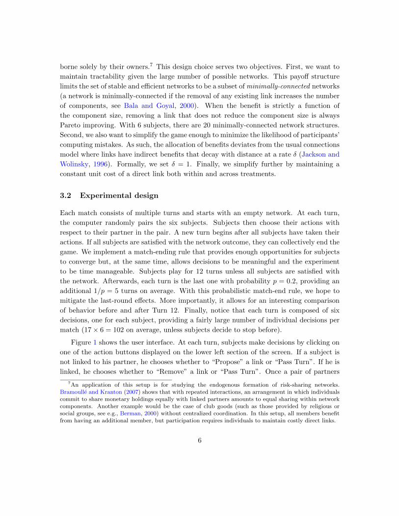
borne solely by their owners.7 This design choice serves two objectives. First, we want to

maintain tractability given the large number of possible networks. This payoff structure

limits the set of stable and efficient networks to be a subset of minimally-connected networks

(a network is minimally-connected if the removal of any existing link increases the number

of components, see Bala and Goyal, 2000). When the benefit is strictly a function of

the component size, removing a link that does not reduce the component size is always

Pareto improving. With 6 subjects, there are 20 minimally-connected network structures.

Second, we also want to simplify the game enough to minimize the likelihood of participants’

computing mistakes. As such, the allocation of benefits deviates from the usual connections

model where links have indirect benefits that decay with distance at a rate δ (Jackson and

Wolinsky, 1996). Formally, we set δ = 1. Finally, we simplify further by maintaining a

constant unit cost of a direct link both within and across treatments.

3.2 Experimental design

Each match consists of multiple turns and starts with an empty network. At each turn,

the computer randomly pairs the six subjects. Subjects then choose their actions with

respect to their partner in the pair. A new turn begins after all subjects have taken their

actions. If all subjects are satisfied with the network outcome, they can collectively end the

game. We implement a match-ending rule that provides enough opportunities for subjects

to converge but, at the same time, allows decisions to be meaningful and the experiment

to be time manageable. Subjects play for 12 turns unless all subjects are satisfied with

the network. Afterwards, each turn is the last one with probability p = 0.2, providing an

additional 1/p = 5 turns on average. With this probabilistic match-end rule, we hope to

mitigate the last-round effects. More importantly, it allows for an interesting comparison

of behavior before and after Turn 12. Finally, notice that each turn is composed of six

decisions, one for each subject, providing a fairly large number of individual decisions per

match (17× 6 = 102 on average, unless subjects decide to stop before).

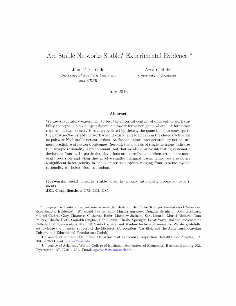
Figure 1 shows the user interface. At each turn, subjects make decisions by clicking on

one of the action buttons displayed on the lower left section of the screen. If a subject is

not linked to his partner, he chooses whether to “Propose” a link or “Pass Turn”. If he is

linked, he chooses whether to “Remove” a link or “Pass Turn”. Once a pair of partners

7An application of this setup is for studying the endogenous formation of risk-sharing networks.Bramoulle and Kranton (2007) shows that with repeated interactions, an arrangement in which individualscommit to share monetary holdings equally with linked partners amounts to equal sharing within networkcomponents. Another example would be the case of club goods (such as those provided by religious orsocial groups, see e.g., Berman, 2000) without centralized coordination. In this setup, all members benefitfrom having an additional member, but participation requires individuals to maintain costly direct links.

6

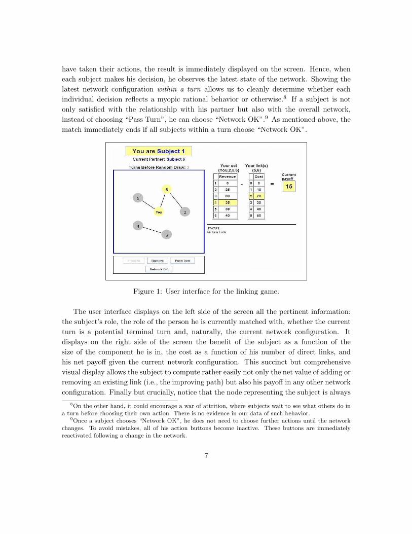
have taken their actions, the result is immediately displayed on the screen. Hence, when

each subject makes his decision, he observes the latest state of the network. Showing the

latest network configuration within a turn allows us to cleanly determine whether each

individual decision reflects a myopic rational behavior or otherwise.8 If a subject is not

only satisfied with the relationship with his partner but also with the overall network,

instead of choosing “Pass Turn”, he can choose “Network OK”.9 As mentioned above, the

match immediately ends if all subjects within a turn choose “Network OK”.

Figure 1: User interface for the linking game.

The user interface displays on the left side of the screen all the pertinent information:

the subject’s role, the role of the person he is currently matched with, whether the current

turn is a potential terminal turn and, naturally, the current network configuration. It

displays on the right side of the screen the benefit of the subject as a function of the

size of the component he is in, the cost as a function of his number of direct links, and

his net payoff given the current network configuration. This succinct but comprehensive

visual display allows the subject to compute rather easily not only the net value of adding or

removing an existing link (i.e., the improving path) but also his payoff in any other network

configuration. Finally but crucially, notice that the node representing the subject is always

8On the other hand, it could encourage a war of attrition, where subjects wait to see what others do ina turn before choosing their own action. There is no evidence in our data of such behavior.

9Once a subject chooses “Network OK”, he does not need to choose further actions until the networkchanges. To avoid mistakes, all of his action buttons become inactive. These buttons are immediatelyreactivated following a change in the network.

7

located at the center and labeled “You”. The nodes representing the other subjects in a

match are labeled by their roles and surround the subject’s node in clockwise order at an

equal distance from it. By always putting the subject’s node at the center, even though

the underlying connections between subjects in a match are identical, each subject sees a

different graphical representation. We therefore avoid leading participants towards focal

networks such as the star or wheel network.

3.3 Treatments

The experiment consists of three main treatments. Figures 4, 5 and 6 illustrate how we de-

sign them. First, we construct a “supernetwork” that contains all 20 minimally-connected

six-node network structures (labeled {A} to {T}). Then, we add all the arcs connecting

pairs of networks that differ from one another by a single link. Network structures are or-

dered from top to bottom based on their number of links and those with identical number

of links are lined up on the same row. Each network is therefore connected by an arc to

one or more networks in the row above and one or more networks in the row below it. The

direction of the arc represents the improving path: forming a new link (arrow pointing to

the row below) or removing an existing link (arrow pointing to the row above).10

Naturally, the improving path depends on the payoffs of each treatment. Contrary to

some existing network experiments, we construct payoff functions that do not follow any

simple functional form. Instead, our payoffs obey two simple restrictions: the benefits are

strictly increasing in component size and the unit cost of a link is constant. This flexibility

simplifies the task of choosing payoffs that can support either no PNS network or a unique

PNS network that is different from the empty or full network and may or may not be

robust to coalition deviations.

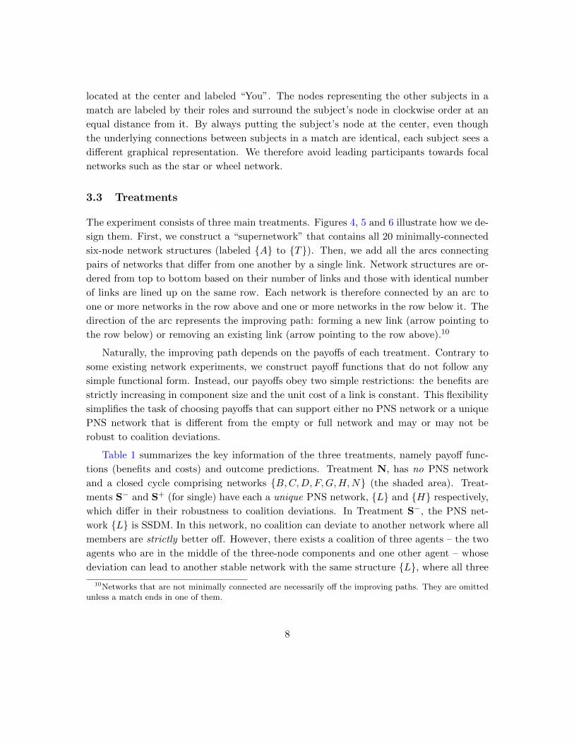
Table 1 summarizes the key information of the three treatments, namely payoff func-

tions (benefits and costs) and outcome predictions. Treatment N, has no PNS network

and a closed cycle comprising networks {B,C,D, F,G,H,N} (the shaded area). Treat-

ments S− and S+ (for single) have each a unique PNS network, {L} and {H} respectively,

which differ in their robustness to coalition deviations. In Treatment S−, the PNS net-

work {L} is SSDM. In this network, no coalition can deviate to another network where all

members are strictly better off. However, there exists a coalition of three agents – the two

agents who are in the middle of the three-node components and one other agent – whose

deviation can lead to another stable network with the same structure {L}, where all three

10Networks that are not minimally connected are necessarily off the improving paths. They are omittedunless a match ends in one of them.

8

agents are weakly better off and one of them is strictly better off. Meanwhile, the PNS

network {H} in Treatment S+ is SSDM and SSJN since no such coalition exists. Network

{H} in Treatment S+ is therefore more robust to coalition deviations than network {L} in

Treatment S−.

To facilitate the comparison of final outcomes across treatments, subjects always start

in the empty network {A} and the efficient networks are always the same: all of the

minimally-connected full networks, that is, {O,P,Q,R, S, T}. We picked multiple efficient

networks with a focal one ({T}, the line that comprises all agents) to give a fair chance to

the efficient outcome.

Table 1: Efficient and stable networks

TreatmentBenefit (size of component) Link

CostPNS SSDM SSJN Efficient

1 2 3 4 5 6

N 0 20 30 39 42 43 15 None None None [6]∗

S− 0 19 36 42 44 45 15 [3-3]{L} [3-3]{L} None [6]∗

S+ 0 29 36 41 43 44 15 [2-2-2]{H} [2-2-2]{H} [2-2-2]{H} [6]∗

Note: The numbers in brackets refer to the size of each component. ∗Includes {O,P,Q,R, S, T}.

Finally, we also considered a fourth treatment with multiple PNS networks, Treat-

ment M. Due to a computation error during programming, instead of the intended two

stable networks (one SSDM and one SSJN), our configuration had two pairwise-stable net-

works, one PNS network and one SSDM network. This complicates the data analysis and

pollutes the comparisons with the other treatments. We therefore decided to concentrate

on Treatments N, S−, and S+ and relegate a brief analysis of Treatment M to Appendix A.

3.4 Implementation

The experiment was conducted in the California Social Science Experimental Laboratory

at UCLA. All experimental subjects were UCLA students. We conducted 8 experimental

sessions with 12 subjects in each session. With 12 subjects, there are always 2 groups of 6

subjects in each session, playing simultaneously 2 matches. Each subject played each of the

four treatments twice. We shuffled the order of the treatments to neutralize the possible

effects from the ordering within a session.11 The analysis in the main text utilizes a total

11Specifically, the order of the treatments is such that: (i) the orders of the treatments in the first half andthe second half of each session were different; (ii) no two sessions have identical treatment sequences; and

9

of 96 match observations (32 matches of treatments N, S−, and S+) from 96 subjects (12

subjects in 8 sessions). The analysis in the appendix utilizes 32 match observations (the

remaining treatment) from the same subjects.

To introduce anonymity in game play, after each match we reshuffled subjects into new

groups and assigned a new role (1 to 6) to each subject. Each session lasted between 90

and 120 minutes. No subject took part in more than one session. Participants interacted

exclusively through computer terminals without knowing the identities of the subjects

they played with. Before the paid matches, instructions were read aloud and two practice

matches were played to familiarize participants with the computer interface and procedure.

After that, participants had to complete a quiz to ensure they understood the rules of the

experiment.

At the end of each match, subjects obtained a payoff based on the size of the component

they were in (benefit) and the number of direct links (cost). Participants were endowed

with experimental tokens and they could earn or lose tokens. At the end of the session,

the payoffs in tokens accumulated from all experimental games were converted into cash,

at the exchange rate of 4 tokens = $1. Participants received a show-up fee of $5, plus the

amount they accumulated during the paid matches. Payments were made in cash and in

private. Matches lasted between 13 and 36 turns, with an average of 16.8 turns. There was

a significant spread in winnings: including the show-up fee, participants earned between

$11 and $43 with an average of $29. A copy of the instructions is included in Appendix C.

4 Network outcomes

This section reports the results on network outcomes. First, we show evidence on the

predictions that link pairwise stability to the outcome of the dynamic linking game that

were derived by Jackson and Watts (2002). Next, we compare the predictive powers of

unique PNS networks whose stability differ in their “strength”. The results of our analysis

are based on the final network outcomes and those conditional on convergence. We employ

the operational definition of convergence suggested by Callander and Plott (2005), as the

lack of change in the final T = 3 turns.12

Before describing the main results, we first study whether our subjects understand the

basic tenets of the game. Table 2 shows that subjects consistently avoid networks that are

not minimally connected. As discussed above, removing a link that does not reduce the

(iii) each treatment was implemented in exactly two (out of eight) sessions for each order in the sequence.12T = 3 is arbitrary. It corresponds to 18 individual decisions which seems reasonably large. With a

larger T , convergence decreases but the qualitative conclusions are very similar (T = 5 is not presented forbrevity but it is available from the authors).

10

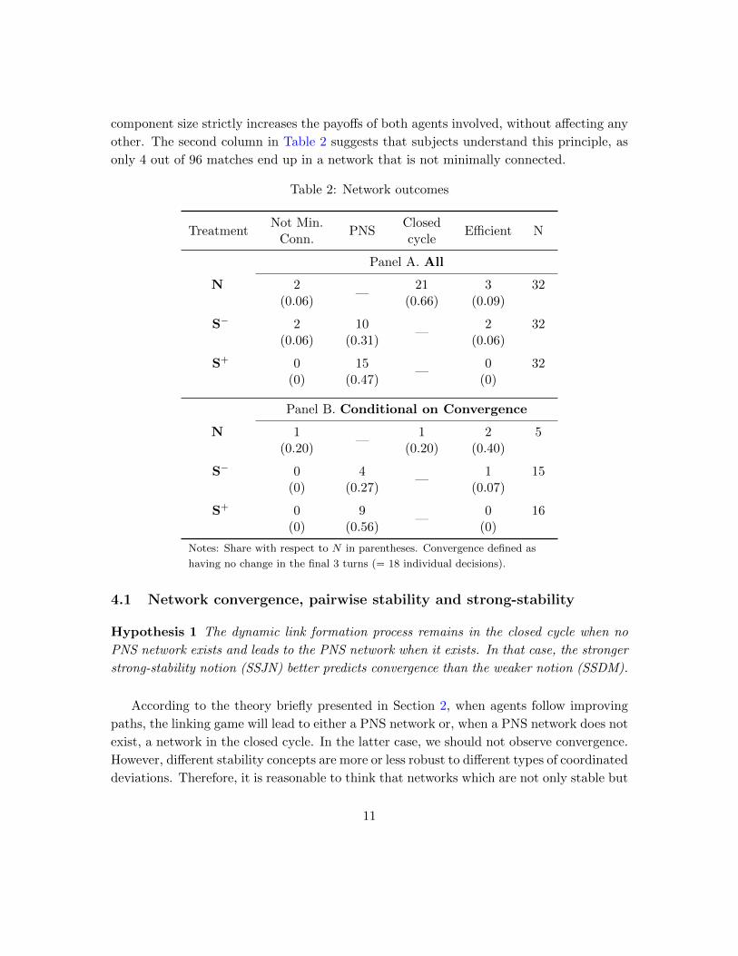
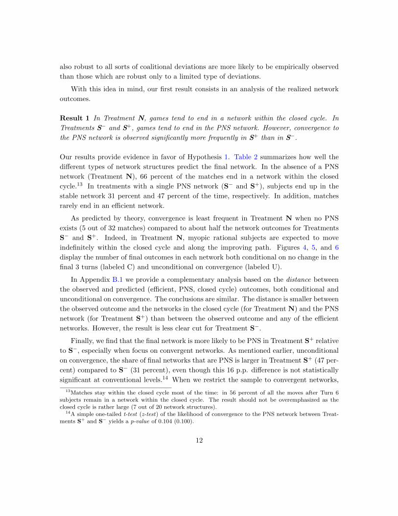
component size strictly increases the payoffs of both agents involved, without affecting any

other. The second column in Table 2 suggests that subjects understand this principle, as

only 4 out of 96 matches end up in a network that is not minimally connected.

Table 2: Network outcomes

TreatmentNot Min.

Conn.PNS

Closedcycle

Efficient N

Panel A. All

N 2—

21 3 32(0.06) (0.66) (0.09)

S− 2 10—

2 32(0.06) (0.31) (0.06)

S+ 0 15—

0 32(0) (0.47) (0)

Panel B. Conditional on Convergence

N 1—

1 2 5(0.20) (0.20) (0.40)

S− 0 4—

1 15(0) (0.27) (0.07)

S+ 0 9—

0 16(0) (0.56) (0)

Notes: Share with respect to N in parentheses. Convergence defined as

having no change in the final 3 turns (= 18 individual decisions).

4.1 Network convergence, pairwise stability and strong-stability

Hypothesis 1 The dynamic link formation process remains in the closed cycle when no

PNS network exists and leads to the PNS network when it exists. In that case, the stronger

strong-stability notion (SSJN) better predicts convergence than the weaker notion (SSDM).

According to the theory briefly presented in Section 2, when agents follow improving

paths, the linking game will lead to either a PNS network or, when a PNS network does not

exist, a network in the closed cycle. In the latter case, we should not observe convergence.

However, different stability concepts are more or less robust to different types of coordinated

deviations. Therefore, it is reasonable to think that networks which are not only stable but

11

also robust to all sorts of coalitional deviations are more likely to be empirically observed

than those which are robust only to a limited type of deviations.

With this idea in mind, our first result consists in an analysis of the realized network

outcomes.

Result 1 In Treatment N, games tend to end in a network within the closed cycle. In

Treatments S− and S+, games tend to end in the PNS network. However, convergence to

the PNS network is observed significantly more frequently in S+ than in S−.

Our results provide evidence in favor of Hypothesis 1. Table 2 summarizes how well the

different types of network structures predict the final network. In the absence of a PNS

network (Treatment N), 66 percent of the matches end in a network within the closed

cycle.13 In treatments with a single PNS network (S− and S+), subjects end up in the

stable network 31 percent and 47 percent of the time, respectively. In addition, matches

rarely end in an efficient network.

As predicted by theory, convergence is least frequent in Treatment N when no PNS

exists (5 out of 32 matches) compared to about half the network outcomes for Treatments

S− and S+. Indeed, in Treatment N, myopic rational subjects are expected to move

indefinitely within the closed cycle and along the improving path. Figures 4, 5, and 6

display the number of final outcomes in each network both conditional on no change in the

final 3 turns (labeled C) and unconditional on convergence (labeled U).

In Appendix B.1 we provide a complementary analysis based on the distance between

the observed and predicted (efficient, PNS, closed cycle) outcomes, both conditional and

unconditional on convergence. The conclusions are similar. The distance is smaller between

the observed outcome and the networks in the closed cycle (for Treatment N) and the PNS

network (for Treatment S+) than between the observed outcome and any of the efficient

networks. However, the result is less clear cut for Treatment S−.

Finally, we find that the final network is more likely to be PNS in Treatment S+ relative

to S−, especially when focus on convergent networks. As mentioned earlier, unconditional

on convergence, the share of final networks that are PNS is larger in Treatment S+ (47 per-

cent) compared to S− (31 percent), even though this 16 p.p. difference is not statistically

significant at conventional levels.14 When we restrict the sample to convergent networks,

13Matches stay within the closed cycle most of the time: in 56 percent of all the moves after Turn 6subjects remain in a network within the closed cycle. The result should not be overemphasized as theclosed cycle is rather large (7 out of 20 network structures).

14A simple one-tailed t-test (z-test) of the likelihood of convergence to the PNS network between Treat-ments S+ and S− yields a p-value of 0.104 (0.100).

12

however, this difference increases to 56 − 27 = 29 p.p. (Panel B of Table 2) and is statis-

tically significant.15 This difference in the likelihood of convergence to the PNS between

Treatments S+ and S− is intriguing. Our result suggests that the disparity may be rooted

in the differences in strength of the stability between network {H} in Treatment S+ and

network {L} in Treatment S−. While the former is robust to coalition deviations by a set

of agents where some are strictly better-off and others weakly better-off (SSJN), the latter

is only robust to coalition deviations by agents who are all strictly better-off (SSDM).

The difference between these two stability concepts may seem minor, but it is not.

Indeed, a property of any (non-connected) SSJN network is that the value of each compo-

nent is equally distributed among its members. This is called component-wise egalitarian

allocation rule (Jackson and van den Nouweland, 2005), and it is not shared by SSDM

networks. In our game, it means that the payoff symmetry of the [2-2-2] network {H} in

Treatment S+ ensures that, once it is reached, there is simply no room for improvement

for any subject. By contrast, the [3-3] network {L} in Treatment S− is only SSDM and

therefore does not satisfy this property. In particular, the two agents at the center of each

component have strong incentives to deviate, in the hope of reaching later on the same

configuration but with someone else bearing the cost of two links.16

4.2 Payoffs

Table 3 presents the mean payoffs obtained by subjects in each treatment. These values are

compared with the average of the mean payoffs had they ended in a network in the closed

cycle (Treatment N) and in the unique PNS network (Treatments S− and S+). We also

compare them to the payoffs in the efficient networks. We find significant losses relative to

the payoffs that could be collectively obtained: empirical payoffs are between 46 percent

and 71 percent of the payoffs generated by the efficient networks. It means that playing

non-cooperatively comes at a substantial cost. In fact, the observed payoffs are smaller but

close to the payoffs in the unique PNS network for Treatments S− and S+. The results are

similar when we consider only the empirical payoffs of the convergent networks. Finally,

the payoffs for Treatment N are 50 percent higher than the average payoffs in the closed

15Assuming observational independence, a one-tailed t-test of the difference in the mean shares of the PNSfinal network among convergent networks has a p-value of 0.051. Since participants are reshuffled betweenmatches within a session, this independence assumption may not hold. Using a t-test with standard errorsthat are clustered at the session level, we obtain a p-value of 0.095. Obviously, these effects are impreciselyestimated in part due to the the small number of match-level observations.

16The only case where subjects in an SSJN network do not obtain the same payoff is when the SSJNnetwork is fully connected (Jackson and van den Nouweland, 2005). The reason why such network is stillSSJN is simply that there is no other component that subjects can join to improve their payoff.

13

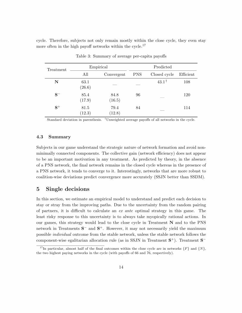
cycle. Therefore, subjects not only remain mostly within the close cycle, they even stay

more often in the high payoff networks within the cycle.17

Table 3: Summary of average per-capita payoffs

TreatmentEmpirical Predicted

All Convergent PNS Closed cycle Efficient

N 63.1— —

43.1 † 108(26.6)

S− 85.4 84.8 96—

120(17.9) (16.5)

S+ 81.5 79.4 84—

114(12.3) (12.8)

Standard deviation in parenthesis. †Unweighted average payoffs of all networks in the cycle.

4.3 Summary

Subjects in our game understand the strategic nature of network formation and avoid non-

minimally connected components. The collective gain (network efficiency) does not appear

to be an important motivation in any treatment. As predicted by theory, in the absence

of a PNS network, the final network remains in the closed cycle whereas in the presence of

a PNS network, it tends to converge to it. Interestingly, networks that are more robust to

coalition-wise deviations predict convergence more accurately (SSJN better than SSDM).

5 Single decisions

In this section, we estimate an empirical model to understand and predict each decision to

stay or stray from the improving paths. Due to the uncertainty from the random pairing

of partners, it is difficult to calculate an ex ante optimal strategy in this game. The

least risky response to this uncertainty is to always take myopically rational actions. In

our games, this strategy would lead to the close cycle in Treatment N and to the PNS

network in Treatments S− and S+. However, it may not necessarily yield the maximum

possible individual outcome from the stable network, unless the stable network follows the

component-wise egalitarian allocation rule (as in SSJN in Treatment S+). Treatment S−

17In particular, almost half of the final outcomes within the close cycle are in networks {F} and {N},the two highest paying networks in the cycle (with payoffs of 66 and 76, respectively).

14

is an example where the maximum individual outcome requires subjects not only to reach

the SSDM, but also be at one end of the network component by the end of the match.

Such a motivation among some subjects in a game may lead to alternative strategies

that do not consist solely of myopic rational actions. We consider two intuitive features of

link formation that might influence these strategies: the end-game rule and the asymmetry

between link formation and link deletion. With regards to the former, with 12 guaran-

teed turns, subjects may be more willing to play riskier strategies earlier in the game.

Meanwhile, the latter may motivate subjects to deviate from myopic rationality mainly

by accumulating extra links, since link deletion can be implemented unilaterally whereas

link formation requires mutual consent. Lastly, the willingness to experiment by straying

from the improving paths may also be influenced by the potential loss from that particular

deviation.

5.1 Descriptive statistics

At each turn, each subject in a pair must choose to either “act” or “pass”. If subjects in the

pair are initially unlinked, acting implies proposing a link and passing implies remaining

unlinked. If subjects are initially linked instead, acting implies removing a link and passing

implies remaining linked. We are interested in the extent to which actions are myopic

rational in each of these four cases and for each treatment.

Table 4 summarizes the proportion of myopic rational actions across turns. We organize

the data into four groups of turns. We use the last certain turn that subjects get unless

everyone agrees on the network outcome (Turn 12) as a natural point to partition and

further split each of these partitions into two. This split captures behaviors at different

stages. First, subjects attempt to get familiar with the current match and try different

strategies which, with high probability, can be reversed later if desired (Turns [1-6]). Then,

subjects adjust their behavior as the last certain turn approaches (Turns [7-12]). After

that, subjects enter the random stopping phase where, presumably, they behave under the

assumption that matches can be terminated at any time (Turns [13-18]). Finally, Turns 19

and above are set in a another category because the sample size is dramatically reduced as

turns advance and the sample becomes non-representative of the population.18

Although formal tests are presented in the regression analysis of Section 5.2, Table 4 is

instructive. Panel A suggests a statistically significant upward jump in myopic rationality

when subjects enter the probabilistic match-ending phase (between [7-12] and [13-18]).

18The split is arbitrary. Similar results are obtained if the first and third partition are changed marginally.The key issue is to introduce a separation at Turn 12.

15

Panel B investigates myopic rationality by type of decision. We examine choices under

four mutually exclusive conditions, namely when the rational action is: (i) to pass and stay

unlinked; (ii) to pass and stay linked; (iii) to remove an existing link; and (iv) to propose

a new link. By comparing conditions (i) with (ii), and (iii) with (iv), we find evidence

that individuals deviate more from improving paths in decisions that reduce the number of

links than in decisions that increase the number of links. By comparing conditions (i) with

(iii), and (ii) with (iv), subjects deviate more by being “over-passive” (failing to act when

they should) than “over-active” (acting when they should not).19 However, our regressions

below suggest that this last result does not hold once we control for subject fixed effects

and the marginal payoff from myopic rational choices. Panel C displays myopic rationality

across treatments and confirms the results of panel A: in all three treatments, subjects are

significantly less myopic rational before Turn 12 than after Turn 12 at the 0.1 percent level.

A graphical illustration of the results in panels B and C is presented for every turn of the

game (up to Turn 18) in Appendix B.2.

Finally, Table 5 presents the number of instances in which subjects choose to “enter”,

“stay” and “leave” the PNS network, broken down by treatment and turn. The last column

reports the total number of turns in that set. We notice that subjects are prone to leave

the PNS network in Turns [1-12], but this tendency is dramatically reduced when each

turn can be final, especially for Treatment S+.

5.2 Empirical framework

5.2.1 Specification

As a formal test, we estimate a linear probability model (LPM) with individual fixed

effects and regress the probability that a subject chooses the myopic rational action on the

attributes of the problem.20 For each treatment, we estimate the following specification:

P(Y ijnt = 1 | Xij

nt, cn) = β0 + Xijnt β + cn (1)

where Y ijnt indicates whether the action that moves subject n from network i to network j

in the supernetwork at Turn t is myopic rational (= 1) or not (= 0), and Xijnt captures the

19A set of t-tests (not reported for brevity) confirms that for each turn group, the mean differences inmyopic rationality both between conditions (i) and (iii) and between conditions (ii) and (iv) are negativeand statistically significant at the 0.1 percent level.

20We choose LPM with fixed-effects instead of a Logit model because its coefficients are easier to interpret,especially in the presence of interaction terms where the derivation of marginal effects can be non-trivial(Ai and Norton, 2003; Greene, 2010). We do not consider the fixed-effects Probit model given its knownbias (Greene, 2004).

16

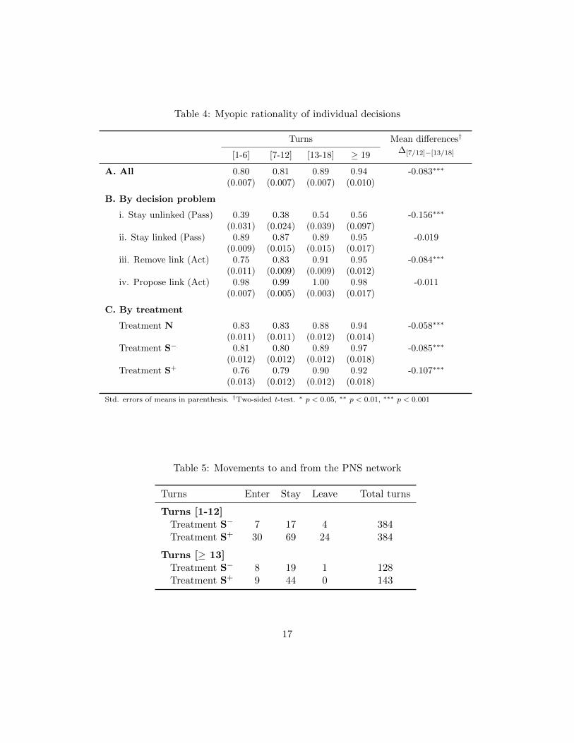
Table 4: Myopic rationality of individual decisions

Turns Mean differences†

∆[7/12]−[13/18][1-6] [7-12] [13-18] ≥ 19

A. All 0.80 0.81 0.89 0.94 -0.083∗∗∗

(0.007) (0.007) (0.007) (0.010)

B. By decision problem

i. Stay unlinked (Pass) 0.39 0.38 0.54 0.56 -0.156∗∗∗

(0.031) (0.024) (0.039) (0.097)ii. Stay linked (Pass) 0.89 0.87 0.89 0.95 -0.019

(0.009) (0.015) (0.015) (0.017)iii. Remove link (Act) 0.75 0.83 0.91 0.95 -0.084∗∗∗

(0.011) (0.009) (0.009) (0.012)iv. Propose link (Act) 0.98 0.99 1.00 0.98 -0.011

(0.007) (0.005) (0.003) (0.017)

C. By treatment

Treatment N 0.83 0.83 0.88 0.94 -0.058∗∗∗

(0.011) (0.011) (0.012) (0.014)Treatment S− 0.81 0.80 0.89 0.97 -0.085∗∗∗

(0.012) (0.012) (0.012) (0.018)Treatment S+ 0.76 0.79 0.90 0.92 -0.107∗∗∗

(0.013) (0.012) (0.012) (0.018)

Std. errors of means in parenthesis. †Two-sided t-test. ∗ p < 0.05, ∗∗ p < 0.01, ∗∗∗ p < 0.001

Table 5: Movements to and from the PNS network

Turns Enter Stay Leave Total turns

Turns [1-12]Treatment S− 7 17 4 384Treatment S+ 30 69 24 384

Turns [≥ 13]Treatment S− 8 19 1 128Treatment S+ 9 44 0 143

17

vector of attributes. Meanwhile, cn captures the unobservable characteristics of subject

n which may affect how she makes decisions. We do not assume that the unobservable

individual characteristics are independent from the attributes of the decisions, and hence,

implement an individual fixed effects specification. The standard errors are clustered by

session. At the end of the section, we briefly discuss some extensions and alternative

representations.

We can use the regression framework to investigate the four types of decisions described

in Panel B of Table 4. Consider first the following simple specification:

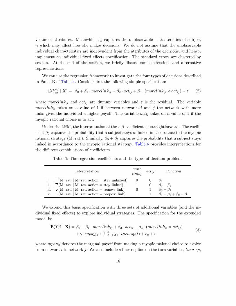
E(Y ijnt | X) = β0 + β1 ·morelinkij + β2 · actij + β3 · (morelinkij × actij) + ε (2)

where morelinkij and actij are dummy variables and ε is the residual. The variable

morelinkij takes on a value of 1 if between networks i and j the network with more

links gives the individual a higher payoff. The variable actij takes on a value of 1 if the

myopic rational choice is to act.

Under the LPM, the interpretation of these β-coefficients is straightforward. The coeffi-

cient β0 captures the probability that a subject stays unlinked in accordance to the myopic

rational strategy (M. rat.). Similarly, β0 + β1 captures the probability that a subject stays

linked in accordance to the myopic rational strategy. Table 6 provides interpretations for

the different combinations of coefficients.

Table 6: The regression coefficients and the types of decision problems

Interpretationmore

actij Functionlinkij

i. P(M. rat. | M. rat. action = stay unlinked) 0 0 β0ii. P(M. rat. | M. rat. action = stay linked) 1 0 β0 + β1iii. P(M. rat. | M. rat. action = remove link) 0 1 β0 + β2iv. P(M. rat. | M. rat. action = propose link) 1 1 β0 + β1 + β2 + β3

We extend this basic specification with three sets of additional variables (and the in-

dividual fixed effects) to explore individual strategies. The specification for the extended

model is:

E(Y ijnt | X) = β0 + β1 ·morelinkij + β2 · actij + β3 · (morelinkij × actij)

+ γ ·mpayij +∑4

t=1 χt · turn sp(t) + cn + ε(3)

where mpayij denotes the marginal payoff from making a myopic rational choice to evolve

from network i to network j. We also include a linear spline on the turn variables, turn sp,

18

with knots at turns 6, 12, and 18 to control for possible turn effects.21 The knot choices

mimic the turn grouping we did for the descriptive analysis.

5.2.2 Hypothesis and results

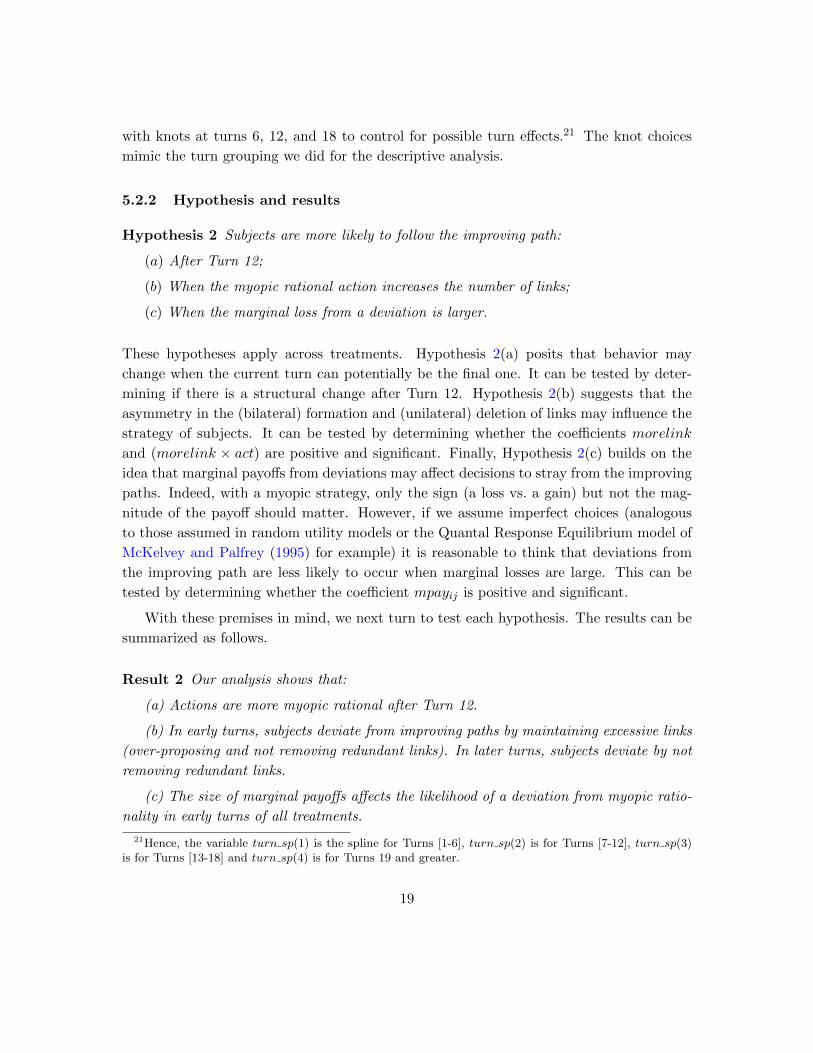
Hypothesis 2 Subjects are more likely to follow the improving path:

(a) After Turn 12;

(b) When the myopic rational action increases the number of links;

(c) When the marginal loss from a deviation is larger.

These hypotheses apply across treatments. Hypothesis 2(a) posits that behavior may

change when the current turn can potentially be the final one. It can be tested by deter-

mining if there is a structural change after Turn 12. Hypothesis 2(b) suggests that the

asymmetry in the (bilateral) formation and (unilateral) deletion of links may influence the

strategy of subjects. It can be tested by determining whether the coefficients morelink

and (morelink × act) are positive and significant. Finally, Hypothesis 2(c) builds on the

idea that marginal payoffs from deviations may affect decisions to stray from the improving

paths. Indeed, with a myopic strategy, only the sign (a loss vs. a gain) but not the mag-

nitude of the payoff should matter. However, if we assume imperfect choices (analogous

to those assumed in random utility models or the Quantal Response Equilibrium model of

McKelvey and Palfrey (1995) for example) it is reasonable to think that deviations from

the improving path are less likely to occur when marginal losses are large. This can be

tested by determining whether the coefficient mpayij is positive and significant.

With these premises in mind, we next turn to test each hypothesis. The results can be

summarized as follows.

Result 2 Our analysis shows that:

(a) Actions are more myopic rational after Turn 12.

(b) In early turns, subjects deviate from improving paths by maintaining excessive links

(over-proposing and not removing redundant links). In later turns, subjects deviate by not

removing redundant links.

(c) The size of marginal payoffs affects the likelihood of a deviation from myopic ratio-

nality in early turns of all treatments.

21Hence, the variable turn sp(1) is the spline for Turns [1-6], turn sp(2) is for Turns [7-12], turn sp(3)is for Turns [13-18] and turn sp(4) is for Turns 19 and greater.

19

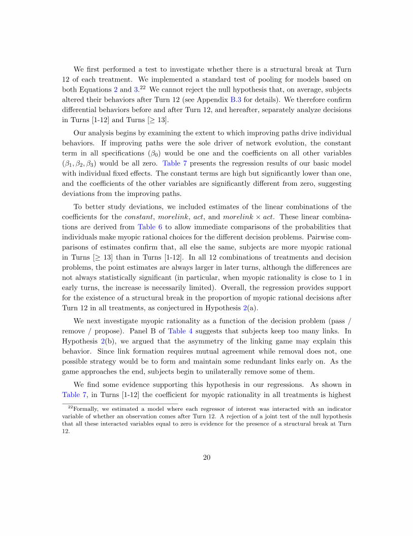
We first performed a test to investigate whether there is a structural break at Turn

12 of each treatment. We implemented a standard test of pooling for models based on

both Equations 2 and 3.22 We cannot reject the null hypothesis that, on average, subjects

altered their behaviors after Turn 12 (see Appendix B.3 for details). We therefore confirm

differential behaviors before and after Turn 12, and hereafter, separately analyze decisions

in Turns [1-12] and Turns [≥ 13].

Our analysis begins by examining the extent to which improving paths drive individual

behaviors. If improving paths were the sole driver of network evolution, the constant

term in all specifications (β0) would be one and the coefficients on all other variables

(β1, β2, β3) would be all zero. Table 7 presents the regression results of our basic model

with individual fixed effects. The constant terms are high but significantly lower than one,

and the coefficients of the other variables are significantly different from zero, suggesting

deviations from the improving paths.

To better study deviations, we included estimates of the linear combinations of the

coefficients for the constant, morelink, act, and morelink × act. These linear combina-

tions are derived from Table 6 to allow immediate comparisons of the probabilities that

individuals make myopic rational choices for the different decision problems. Pairwise com-

parisons of estimates confirm that, all else the same, subjects are more myopic rational

in Turns [≥ 13] than in Turns [1-12]. In all 12 combinations of treatments and decision

problems, the point estimates are always larger in later turns, although the differences are

not always statistically significant (in particular, when myopic rationality is close to 1 in

early turns, the increase is necessarily limited). Overall, the regression provides support

for the existence of a structural break in the proportion of myopic rational decisions after

Turn 12 in all treatments, as conjectured in Hypothesis 2(a).

We next investigate myopic rationality as a function of the decision problem (pass /

remove / propose). Panel B of Table 4 suggests that subjects keep too many links. In

Hypothesis 2(b), we argued that the asymmetry of the linking game may explain this

behavior. Since link formation requires mutual agreement while removal does not, one

possible strategy would be to form and maintain some redundant links early on. As the

game approaches the end, subjects begin to unilaterally remove some of them.

We find some evidence supporting this hypothesis in our regressions. As shown in

Table 7, in Turns [1-12] the coefficient for myopic rationality in all treatments is highest

22Formally, we estimated a model where each regressor of interest was interacted with an indicatorvariable of whether an observation comes after Turn 12. A rejection of a joint test of the null hypothesisthat all these interacted variables equal to zero is evidence for the presence of a structural break at Turn12.

20

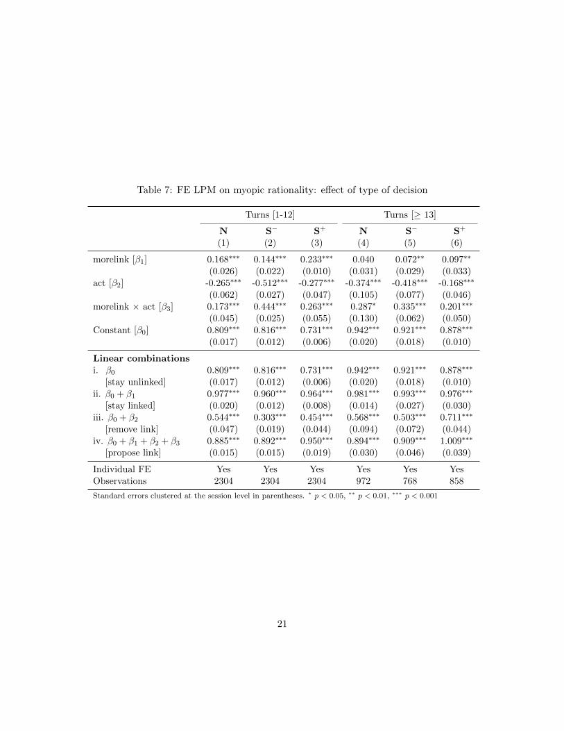
Table 7: FE LPM on myopic rationality: effect of type of decision

Turns [1-12] Turns [≥ 13]

N S− S+ N S− S+

(1) (2) (3) (4) (5) (6)

morelink [β1] 0.168∗∗∗ 0.144∗∗∗ 0.233∗∗∗ 0.040 0.072∗∗ 0.097∗∗

(0.026) (0.022) (0.010) (0.031) (0.029) (0.033)act [β2] -0.265∗∗∗ -0.512∗∗∗ -0.277∗∗∗ -0.374∗∗∗ -0.418∗∗∗ -0.168∗∗∗

(0.062) (0.027) (0.047) (0.105) (0.077) (0.046)morelink × act [β3] 0.173∗∗∗ 0.444∗∗∗ 0.263∗∗∗ 0.287∗ 0.335∗∗∗ 0.201∗∗∗

(0.045) (0.025) (0.055) (0.130) (0.062) (0.050)Constant [β0] 0.809∗∗∗ 0.816∗∗∗ 0.731∗∗∗ 0.942∗∗∗ 0.921∗∗∗ 0.878∗∗∗

(0.017) (0.012) (0.006) (0.020) (0.018) (0.010)

Linear combinationsi. β0

[stay unlinked]0.809∗∗∗ 0.816∗∗∗ 0.731∗∗∗ 0.942∗∗∗ 0.921∗∗∗ 0.878∗∗∗

(0.017) (0.012) (0.006) (0.020) (0.018) (0.010)ii. β0 + β1

[stay linked]0.977∗∗∗ 0.960∗∗∗ 0.964∗∗∗ 0.981∗∗∗ 0.993∗∗∗ 0.976∗∗∗

(0.020) (0.012) (0.008) (0.014) (0.027) (0.030)iii. β0 + β2

[remove link]0.544∗∗∗ 0.303∗∗∗ 0.454∗∗∗ 0.568∗∗∗ 0.503∗∗∗ 0.711∗∗∗

(0.047) (0.019) (0.044) (0.094) (0.072) (0.044)iv. β0 + β1 + β2 + β3

[propose link]0.885∗∗∗ 0.892∗∗∗ 0.950∗∗∗ 0.894∗∗∗ 0.909∗∗∗ 1.009∗∗∗

(0.015) (0.015) (0.019) (0.030) (0.046) (0.039)

Individual FE Yes Yes Yes Yes Yes YesObservations 2304 2304 2304 972 768 858

Standard errors clustered at the session level in parentheses. ∗ p < 0.05, ∗∗ p < 0.01, ∗∗∗ p < 0.001

21

when the myopic rational action is to stay linked (ii), followed by propose a link (iv),

stay unlinked (i), and remove a link (iii). For Turns [≥ 13], subjects are most likely to

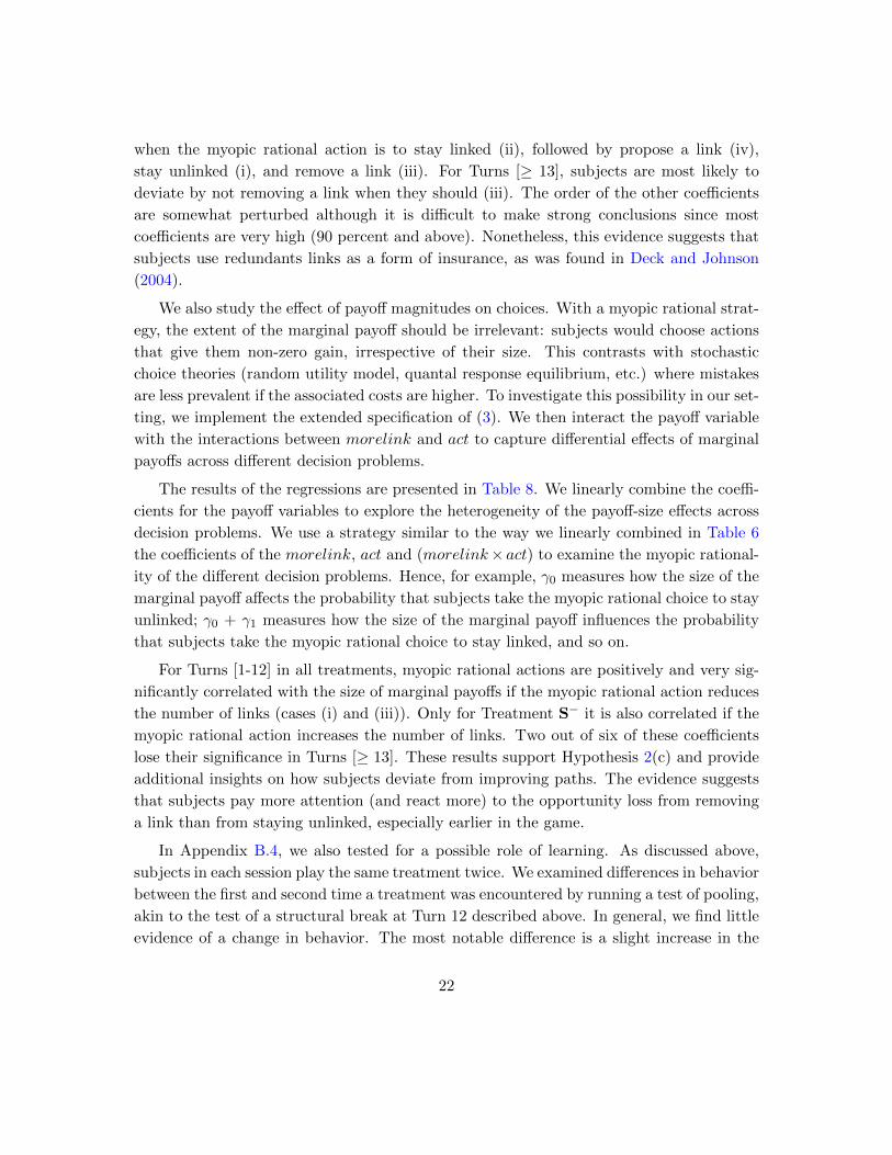
deviate by not removing a link when they should (iii). The order of the other coefficients

are somewhat perturbed although it is difficult to make strong conclusions since most

coefficients are very high (90 percent and above). Nonetheless, this evidence suggests that

subjects use redundants links as a form of insurance, as was found in Deck and Johnson

(2004).

We also study the effect of payoff magnitudes on choices. With a myopic rational strat-

egy, the extent of the marginal payoff should be irrelevant: subjects would choose actions

that give them non-zero gain, irrespective of their size. This contrasts with stochastic

choice theories (random utility model, quantal response equilibrium, etc.) where mistakes

are less prevalent if the associated costs are higher. To investigate this possibility in our set-

ting, we implement the extended specification of (3). We then interact the payoff variable

with the interactions between morelink and act to capture differential effects of marginal

payoffs across different decision problems.

The results of the regressions are presented in Table 8. We linearly combine the coeffi-

cients for the payoff variables to explore the heterogeneity of the payoff-size effects across

decision problems. We use a strategy similar to the way we linearly combined in Table 6

the coefficients of the morelink, act and (morelink× act) to examine the myopic rational-

ity of the different decision problems. Hence, for example, γ0 measures how the size of the

marginal payoff affects the probability that subjects take the myopic rational choice to stay

unlinked; γ0 + γ1 measures how the size of the marginal payoff influences the probability

that subjects take the myopic rational choice to stay linked, and so on.

For Turns [1-12] in all treatments, myopic rational actions are positively and very sig-

nificantly correlated with the size of marginal payoffs if the myopic rational action reduces

the number of links (cases (i) and (iii)). Only for Treatment S− it is also correlated if the

myopic rational action increases the number of links. Two out of six of these coefficients

lose their significance in Turns [≥ 13]. These results support Hypothesis 2(c) and provide

additional insights on how subjects deviate from improving paths. The evidence suggests

that subjects pay more attention (and react more) to the opportunity loss from removing

a link than from staying unlinked, especially earlier in the game.

In Appendix B.4, we also tested for a possible role of learning. As discussed above,

subjects in each session play the same treatment twice. We examined differences in behavior

between the first and second time a treatment was encountered by running a test of pooling,

akin to the test of a structural break at Turn 12 described above. In general, we find little

evidence of a change in behavior. The most notable difference is a slight increase in the

22

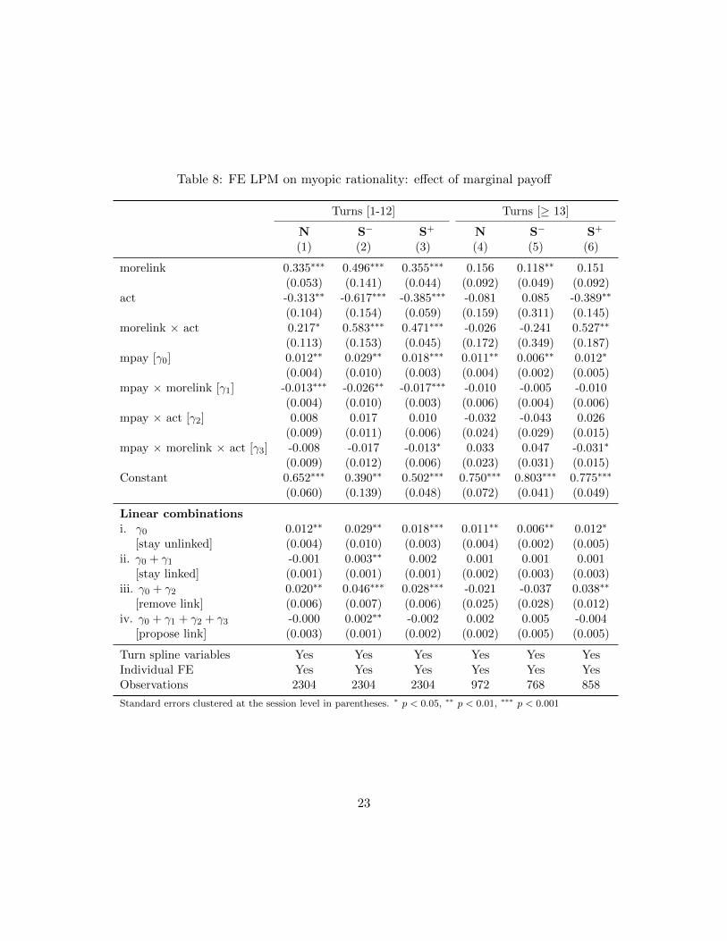
Table 8: FE LPM on myopic rationality: effect of marginal payoff

Turns [1-12] Turns [≥ 13]

N S− S+ N S− S+

(1) (2) (3) (4) (5) (6)

morelink 0.335∗∗∗ 0.496∗∗∗ 0.355∗∗∗ 0.156 0.118∗∗ 0.151(0.053) (0.141) (0.044) (0.092) (0.049) (0.092)

act -0.313∗∗ -0.617∗∗∗ -0.385∗∗∗ -0.081 0.085 -0.389∗∗

(0.104) (0.154) (0.059) (0.159) (0.311) (0.145)morelink × act 0.217∗ 0.583∗∗∗ 0.471∗∗∗ -0.026 -0.241 0.527∗∗

(0.113) (0.153) (0.045) (0.172) (0.349) (0.187)mpay [γ0] 0.012∗∗ 0.029∗∗ 0.018∗∗∗ 0.011∗∗ 0.006∗∗ 0.012∗

(0.004) (0.010) (0.003) (0.004) (0.002) (0.005)mpay × morelink [γ1] -0.013∗∗∗ -0.026∗∗ -0.017∗∗∗ -0.010 -0.005 -0.010

(0.004) (0.010) (0.003) (0.006) (0.004) (0.006)mpay × act [γ2] 0.008 0.017 0.010 -0.032 -0.043 0.026

(0.009) (0.011) (0.006) (0.024) (0.029) (0.015)mpay × morelink × act [γ3] -0.008 -0.017 -0.013∗ 0.033 0.047 -0.031∗

(0.009) (0.012) (0.006) (0.023) (0.031) (0.015)Constant 0.652∗∗∗ 0.390∗∗ 0.502∗∗∗ 0.750∗∗∗ 0.803∗∗∗ 0.775∗∗∗

(0.060) (0.139) (0.048) (0.072) (0.041) (0.049)

Linear combinationsi. γ0

[stay unlinked]0.012∗∗ 0.029∗∗ 0.018∗∗∗ 0.011∗∗ 0.006∗∗ 0.012∗

(0.004) (0.010) (0.003) (0.004) (0.002) (0.005)ii. γ0 + γ1

[stay linked]-0.001 0.003∗∗ 0.002 0.001 0.001 0.001(0.001) (0.001) (0.001) (0.002) (0.003) (0.003)

iii. γ0 + γ2[remove link]

0.020∗∗ 0.046∗∗∗ 0.028∗∗∗ -0.021 -0.037 0.038∗∗

(0.006) (0.007) (0.006) (0.025) (0.028) (0.012)iv. γ0 + γ1 + γ2 + γ3

[propose link]-0.000 0.002∗∗ -0.002 0.002 0.005 -0.004(0.003) (0.001) (0.002) (0.002) (0.005) (0.005)

Turn spline variables Yes Yes Yes Yes Yes YesIndividual FE Yes Yes Yes Yes Yes YesObservations 2304 2304 2304 972 768 858

Standard errors clustered at the session level in parentheses. ∗ p < 0.05, ∗∗ p < 0.01, ∗∗∗ p < 0.001

23

response to marginal losses the second time subjects played Treatment N.

5.3 Model predictions

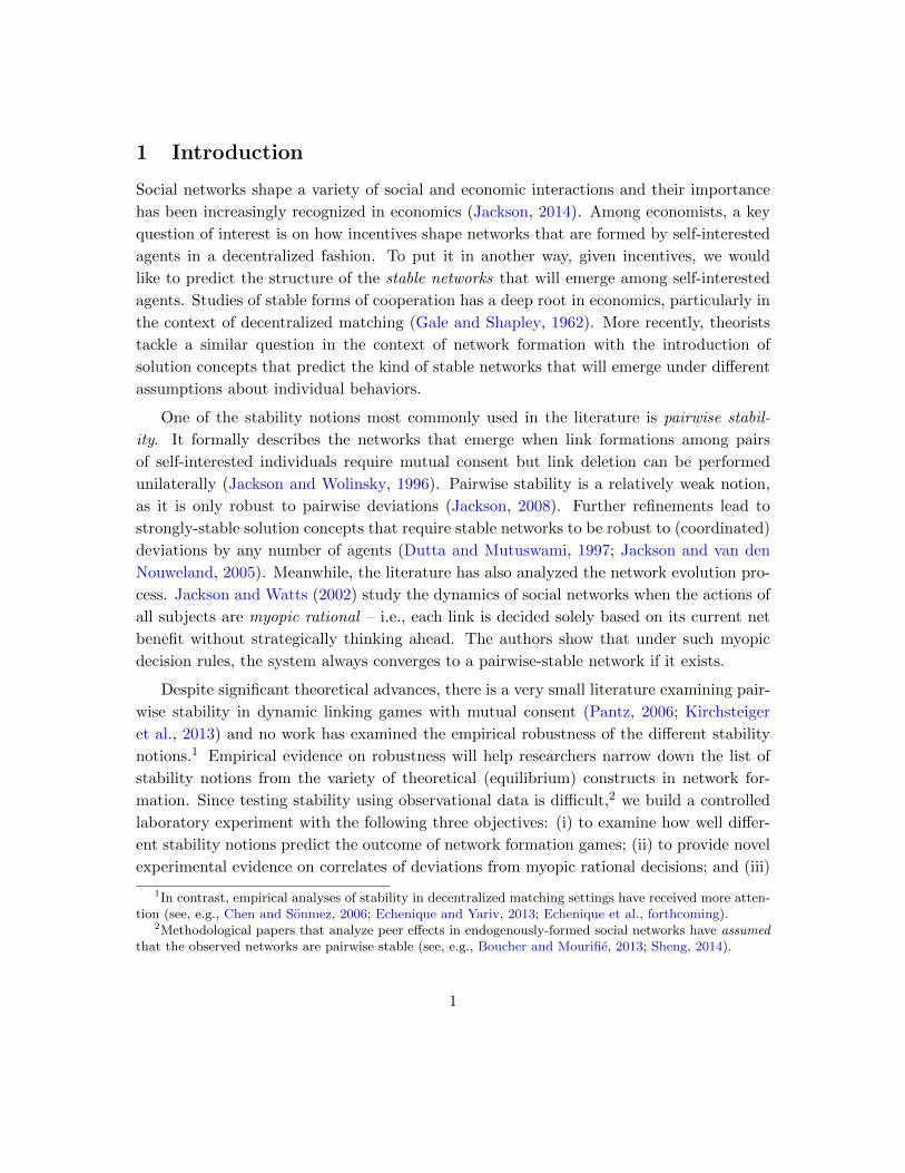
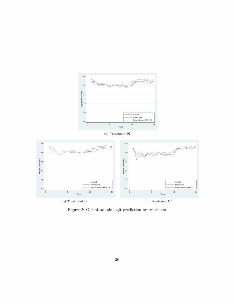
We next examine the capacity of our empirical model to predict actions. Our prediction

model uses a relatively parsimonious specification that incorporates insights from Result 2.

In particular, we estimated a logit model where we supplanted the basic model of Equa-

tion 1 with (i) mpay and (ii) (mpay×morelink) to incorporate Results 2(b) and 2(c). To

incorporate the insight from Result 2(a) and account for the structural break at Turn 12,

all of these variables are interacted with the indicator variable 1(turn > 12). To maintain

model parsimony, we do not include the individual fixed effects.

We use the model to conduct an out-of sample prediction exercise. For each treatment,

we estimated the coefficients of the model with a sample that excludes observations from

that treatment. Once the coefficients are recovered, we use the model to predict the

actions in the excluded treatment. Table 9 shows the coefficients from the estimation

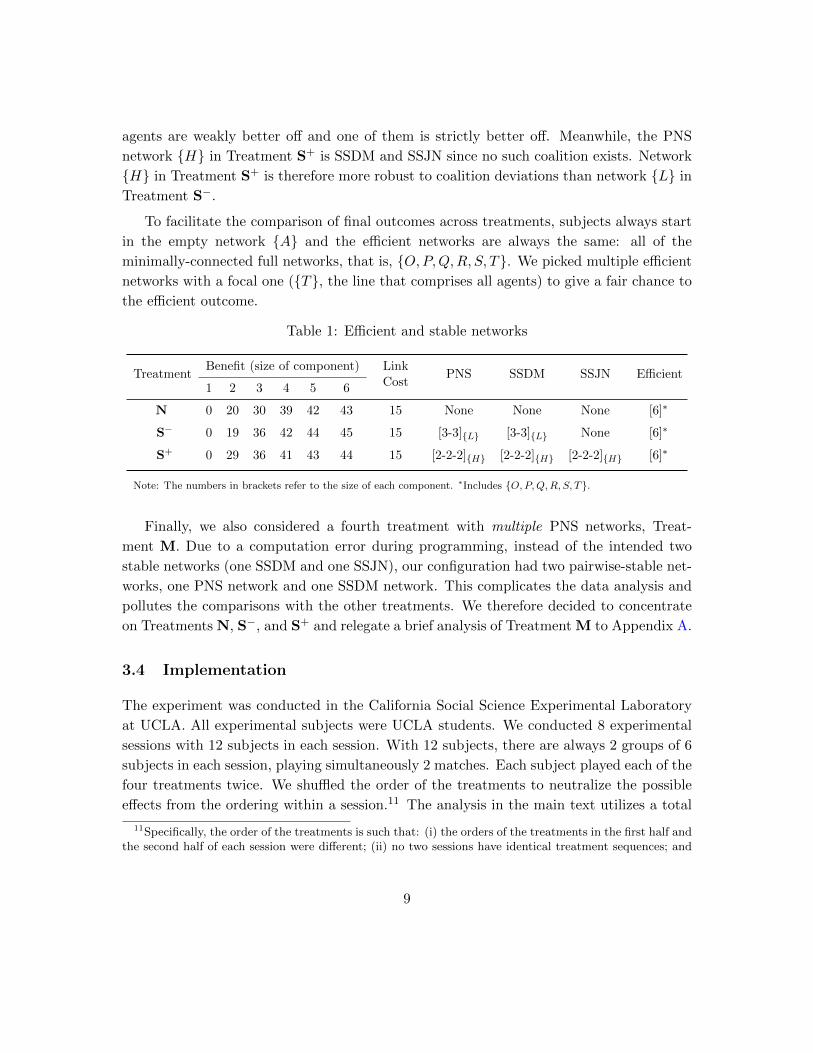
exercise. We then use these coefficients to predict the out-of-sample actions of the first 18

turns. Figure 2 graphically depicts for each treatment the plot of the myopic rationality

of actual choices (dashed line), out-of-sample predicted choices (solid line), and 95 percent

confidence interval of predicted choices.

The model generally predicts actions well, even though it performs less well in predicting

initial behavior and switches around Turn 12. Indeed, in all three treatments actions are

more likely to be outside the prediction intervals in the first few turns and the turns around

Turn 12. However, the absolute differences are always relatively small.

5.4 Summary

The analysis at the single decision level suggests that subjects take for the most part

the myopic rational action. At the same time, we highlight important and systematic

deviations. Indeed, we observe less myopically-rational actions in turns with a sure future

than in random-ending turns. Deviations also tend to take the form of excessive links,

possibly because they can be removed unilaterally, although proving this hypothesis would

require further work. Finally, deviations are also more prevalent the smaller the marginal

payoff losses, as expected in a behavioral theory where “mistakes” (which could be part of

experimentation) depend inversely on loss magnitudes. Overall and with some interesting

exceptions, the analysis provides support for convergence to PNS networks through myopic

rational choices.

24

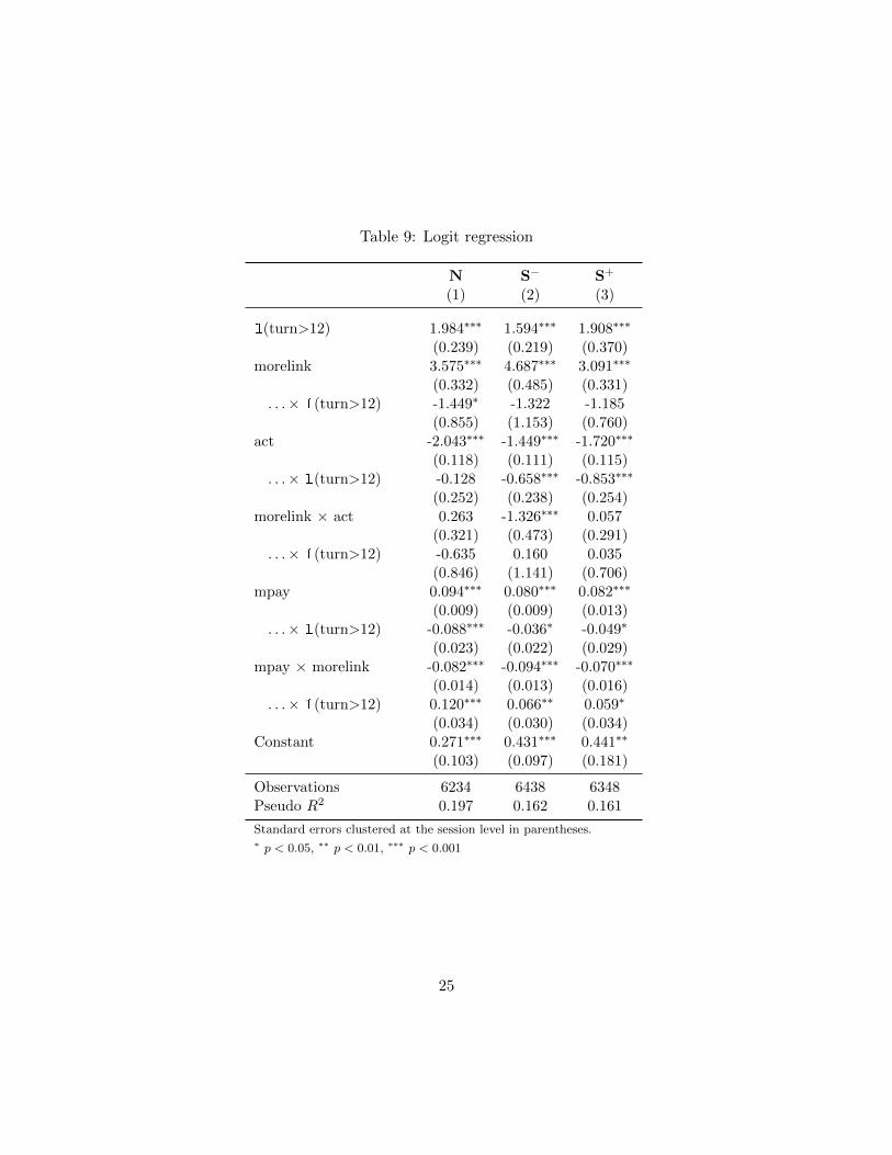
Table 9: Logit regression

N S− S+

(1) (2) (3)

1(turn>12) 1.984∗∗∗ 1.594∗∗∗ 1.908∗∗∗

(0.239) (0.219) (0.370)morelink 3.575∗∗∗ 4.687∗∗∗ 3.091∗∗∗

(0.332) (0.485) (0.331). . .× 1(turn>12) -1.449∗ -1.322 -1.185

(0.855) (1.153) (0.760)act -2.043∗∗∗ -1.449∗∗∗ -1.720∗∗∗

(0.118) (0.111) (0.115). . .× 1(turn>12) -0.128 -0.658∗∗∗ -0.853∗∗∗

(0.252) (0.238) (0.254)morelink × act 0.263 -1.326∗∗∗ 0.057

(0.321) (0.473) (0.291). . .× 1(turn>12) -0.635 0.160 0.035

(0.846) (1.141) (0.706)mpay 0.094∗∗∗ 0.080∗∗∗ 0.082∗∗∗

(0.009) (0.009) (0.013). . .× 1(turn>12) -0.088∗∗∗ -0.036∗ -0.049∗

(0.023) (0.022) (0.029)mpay × morelink -0.082∗∗∗ -0.094∗∗∗ -0.070∗∗∗

(0.014) (0.013) (0.016). . .× 1(turn>12) 0.120∗∗∗ 0.066∗∗ 0.059∗

(0.034) (0.030) (0.034)Constant 0.271∗∗∗ 0.431∗∗∗ 0.441∗∗

(0.103) (0.097) (0.181)

Observations 6234 6438 6348Pseudo R2 0.197 0.162 0.161

Standard errors clustered at the session level in parentheses.∗ p < 0.05, ∗∗ p < 0.01, ∗∗∗ p < 0.001

25

1.8

.6.4

.20

Myo

pic

ratio

nalit

y

0 6 12 18Turn

ActualPredictedUpper/Lower 95% CI

(a) Treatment N

1.8

.6.4

.20

Myo

pic

ratio

nalit

y

0 6 12 18Turn

ActualPredictedUpper/Lower 95% CI

(b) Treatment S−

1.8

.6.4

.20

Myo

pic

ratio

nalit

y

0 6 12 18Turn

ActualPredictedUpper/Lower 95% CI

(c) Treatment S+

Figure 2: Out-of-sample logit prediction by treatment

26

6 Choices by subjects

So far we have analyzed network outcomes and single decisions. One question that remains

unaddressed is the degree of subject heterogeneity. To answer that question, we use cluster

analysis to classify subjects based on their behavior. We implemented the mixture models

approach, which treats each cluster as a component probability distribution and endoge-

nously chooses (optimally) the model and number of clusters using Bayesian statistical

methods (Fraley and Raftery, 2002). In doing so, it avoids the necessity of having to set

the number of clusters and clustering criterion ex ante that was found in alternative clus-

tering approaches. We implement model-based clustering analysis with the mclust package

in R (Fraley et al., 2012). A maximum of nine clusters are considered for up to ten different

models and the combination yielding the maximum Bayesian Information Criterion (BIC)

is chosen.

Since we want to study heterogeneity across subjects in the likelihood of choosing

myopic rational strategies, the variables we use as inputs to the model are guided by the

findings in Result 2: subjects’ level of myopic rationality at early and late turns, and

subjects’ willingness to deviate given the size of the marginal loss, also at early and late

turns. Indeed, our analysis of individual decisions suggests statistically significant jumps

in myopic rationality between early and late turns. To capture subject level variation, we

consider myopic rationality in early turns (1 to 12) and late turns (13 and above) separately.

Meanwhile, to capture the responsiveness of each subject’s deviation to the size of marginal

loss, we estimated a regression akin to Equation (3) for each of the subjects, and use the

subject’s coefficient on the marginal payoff (γ) as this measure of responsiveness to the

marginal loss.23 The coefficients are estimated for early and late turns.

Hypothesis 3 There are three types of subjects: (i) random (with low levels of myopic

rationality), (ii) rational (with high levels of myopic rationality) and (iii) strategic (who

deviate from myopic rationality only when the cost is low). Earnings are lowest for random

subjects and highest for strategic subjects.

We anticipate substantial heterogeneity across individuals. In a game where option

values are difficult to compute, trading-off current costs and benefits (as myopic rationality

predicts) seems a plausible, reasonably sophisticated strategy. Since the game is inherently

difficult, we also expect to observe some subjects to be “lost in the network.” Finally, the

most interesting behavior relates to subjects who realize the appeal of myopic rational

23The equation estimated is slightly different from (3) in that we dropped the turn splines variables andwe allowed the coefficients on the regressors to vary between early and late turns.

27

choices but also try to exploit its shortcomings. These subjects will deviate early in the

game and when the marginal loss is low. They are also expected to accumulate the highest

earnings.

Result 3 We observe 10 percent of random subjects, 25 percent of rational subjects and

65 percent of subjects with two different levels of strategic behavior. Earnings are mono-

tonically increasing in the proportion of myopic rational choices in early turns.

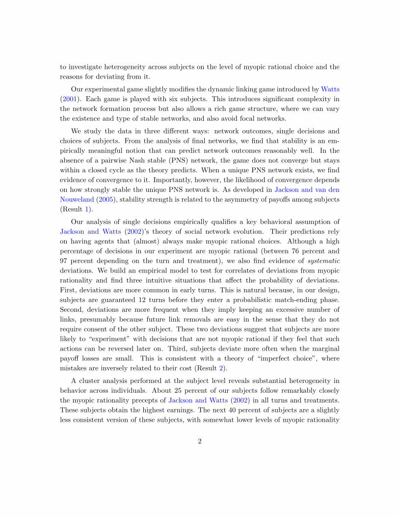
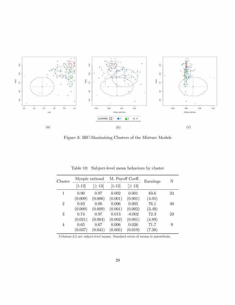
The model endogenously generated four clusters. Figure 3 shows the model’s projec-

tions onto three variable pairs. On the vertical axis, we present the most discriminatory

variable, namely myopic rationality in early turns. On the horizontal axis, we present

each of the other three variables: myopic rationality in late turns (3a); marginal payoff

coefficient in early turns (3b); and marginal payoff coefficient in late turns (3c). Table 10

provides a summary of the mean values of the input variables and earnings within each

cluster, sorted by their mean earnings.

As we can see from Figure 3a and Table 10 (Columns 2-3), the four clusters are clearly

differentiated in terms of the level of myopic rationality in early and late turns. About

25 percent of subjects (Cluster 1) are “rational”: they consistently followed the improving

path throughout the game. On the other end, 10 percent of the subjects (Cluster 4) are

“random”: they often deviate from the improving path, playing the myopic strategy barely

more frequently than predicted by chance. The majority of subjects, around 65 percent

(Clusters 2 and 3), are “strategic”: they explore strategies involving non-myopic rational

choices in early turns before resorting to primarily myopic rational choices in late turns.

Figure 3b and Table 10 (Column 4) suggest that these subjects can be further classified

based on the marginal payoff coefficients in early turns. Indeed, subjects in Cluster 3 are

more likely to use the magnitude of the marginal losses to guide their strategy in early

turns before entirely abandoning it in late turns. In comparison, Cluster 2 subjects rely

less on the marginal payoff coefficient: Their mean level of myopic rationality (marginal

payoff coefficients) are higher (lower) than Cluster 3 subjects’ in early turns, but are stable

throughout the game. Finally, notice from Figure 3c and Table 10 (Column 5) that unlike

the others, subjects in Cluster 4 fail to realize the urgency of making myopic rational

choices following Turn 12. Against the expectation of profit maximizing subjects, they

respond more to marginal losses in later than in earlier turns of the game. This is further

evidence that these subjects do not fully grasp the trade-offs of the game.

Our decomposition exercise confirms the distinctions between clusters whose subjects

consistently followed the improving path, consistently ignored the improving path, and

28

0.5 0.6 0.7 0.8 0.9 1.0

0.5

0.6

0.7

0.8

0.9

Late

Ear

ly

(a)

−0.01 0.00 0.01 0.02

0.5

0.6

0.7

0.8

0.9

M.Pay.Coef.Early

Ear

ly

(b)

−0.05 0.00 0.05 0.10

0.5

0.6

0.7

0.8

0.9

M.Pay.Coef.Late

Ear

ly

(c)

Figure 3: BIC-Maximizing Clusters of the Mixture Models

Table 10: Subject-level mean behaviors by cluster

ClusterMyopic rational M. Payoff Coeff.

Earnings N[1-12] [≥ 13] [1-12] [≥ 13]

1 0.90 0.97 0.002 0.001 83.6 24(0.009) (0.006) (0.001) (0.001) (4.05)

2 0.83 0.86 0.006 0.005 76.1 40(0.009) (0.009) (0.001) (0.002) (3.49)

3 0.74 0.97 0.013 -0.002 72.3 23(0.021) (0.004) (0.002) (0.001) (4.89)

4 0.65 0.67 0.006 0.026 71.7 9(0.037) (0.041) (0.005) (0.019) (7.38)

Columns 2-5 are subject-level means. Standard errors of means in parenthesis.

29

the majority who explored some (early) deviations. In Table 11, we study whether these

differences across clusters are similar in all three treatments. The patterns are remarkably

similar in N, S−, and S+. Perhaps the only noticeable difference is that in Treatment S−

Cluster 2 subjects exhibit a significant increase in myopic rationality between early and

late turns, much like Cluster 3 subjects.

Table 11: Myopic rationality of decisions by cluster and treatment

Cluster 1 2 3 4

Turn [1-12] [13-18] [1-12] [13-18] [1-12] [13-18] [1-12] [13-18]

Treatment

Treatment N 0.88 0.98 0.83 0.86 0.82 0.92 0.71 0.63(0.013) (0.010) (0.012) (0.020) (0.016) (0.020) (0.031) (0.062)

Treatment S− 0.90 0.93 0.82 0.84 0.74 0.96 0.68 0.81(0.013) (0.020) (0.012) (0.022) (0.019) (0.014) (0.032) (0.051)

Treatment S+ 0.91 0.99 0.83 0.87 0.67 0.97 0.56 0.62(0.012) (0.006) (0.012) (0.022) (0.020) (0.013) (0.034) (0.062)

All 0.90 0.97 0.83 0.86 0.74 0.95 0.65 0.68(0.007) (0.008) (0.007) (0.012) (0.011) (0.010) (0.019) (0.034)

Numbers are decision-level means. Standard errors of means in parenthesis.

From Table 10 we also notice that earnings are positively correlated with the proportion

of myopic rational choices in early turns. This contrasts with our hypothesis that the more

strategic subjects – those who do not necessarily take myopic rational decision early in the

game but do it consistently later on – would obtain the highest profits.24

A possible explanation is that payoffs in the game are (very) noisy signals of the strategy

of individuals: It depends on the behavior of the five other subjects in the network and their

final position in the component. The most forward looking subjects may end up bearing

a larger number of links and/or being negatively affected by subjects who use suboptimal

strategies. To investigate the effect of subject composition on network outcomes, we count

for each match the number of subjects from each cluster. We then regress whether the

match ended in a cycle (for Treatment N) or in the PNS network (for Treatments S− and

S+) on the number of subjects from each cluster. Cluster 1, whose subjects’ behavior is

most similar to those assumed in theory, are used as the benchmark and is therefore the

omitted category in the regression. The models are estimated with a session fixed effects

and results are presented in Table 12.

24The result, however, should not be overemphasized since pairwise t-tests do not find statistically sig-nificant differences in mean earnings between clusters except for Cluster 1.

30

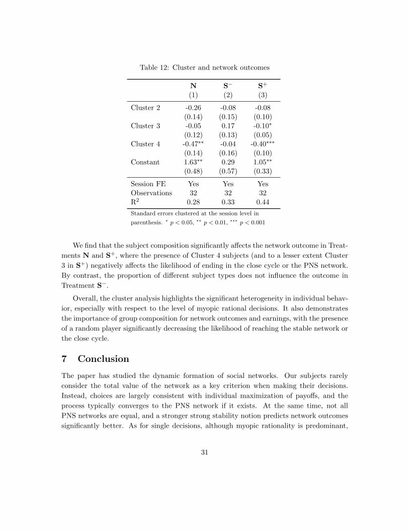
Table 12: Cluster and network outcomes

N S− S+

(1) (2) (3)

Cluster 2 -0.26 -0.08 -0.08(0.14) (0.15) (0.10)

Cluster 3 -0.05 0.17 -0.10∗

(0.12) (0.13) (0.05)Cluster 4 -0.47∗∗ -0.04 -0.40∗∗∗

(0.14) (0.16) (0.10)Constant 1.63∗∗ 0.29 1.05∗∗

(0.48) (0.57) (0.33)

Session FE Yes Yes YesObservations 32 32 32R2 0.28 0.33 0.44

Standard errors clustered at the session level in

parenthesis. ∗ p < 0.05, ∗∗ p < 0.01, ∗∗∗ p < 0.001

We find that the subject composition significantly affects the network outcome in Treat-

ments N and S+, where the presence of Cluster 4 subjects (and to a lesser extent Cluster

3 in S+) negatively affects the likelihood of ending in the close cycle or the PNS network.

By contrast, the proportion of different subject types does not influence the outcome in

Treatment S−.

Overall, the cluster analysis highlights the significant heterogeneity in individual behav-

ior, especially with respect to the level of myopic rational decisions. It also demonstrates

the importance of group composition for network outcomes and earnings, with the presence

of a random player significantly decreasing the likelihood of reaching the stable network or

the close cycle.

7 Conclusion

The paper has studied the dynamic formation of social networks. Our subjects rarely

consider the total value of the network as a key criterion when making their decisions.

Instead, choices are largely consistent with individual maximization of payoffs, and the

process typically converges to the PNS network if it exists. At the same time, not all

PNS networks are equal, and a stronger strong stability notion predicts network outcomes

significantly better. As for single decisions, although myopic rationality is predominant,

31

we also observe interesting systematic deviations from it. In particular, myopic rationality

is less prevalent at the margin when actions are reversible, when marginal payoff losses

are smaller and when actions involve excessive links that can be removed unilaterally later

on. Finally, we also notice a significant heterogeneity in behavior across subjects, with a

majority of subjects deviating from myopic rationality only early in the game.

Despite the recent advances, there is still much to learn about network formation,

both theoretically and experimentally. On the theory front, it would be interesting to

incorporate behavioral imperfections into existing models. The tendency observed in our

data towards fewer deviations from myopic rationality as marginal losses increase and as

matches enter the probabilistic ending phase suggests that subjects optimize subject to

imperfect choice, imperfect foresight and/or imperfect understanding of the game. To

our knowledge, however, no model has yet been developed to capture these frictions. On

the experimental front, ecological validity is a concern. Indeed, we feel that our cost

and benefit representation of adding and removing links captures the essence of social

networks in an excessively stylized and abstract way. The use of laboratory studies in the

field or laboratory studies that exploit social technologies (facebook, twitter, second life,

etc.) would add a more realistic dimension to the network formation problem without

compromising the controlled environment of the laboratory.

32

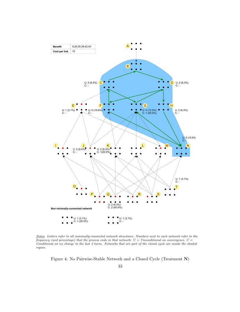
MLKI

N

Non minimally-connected network

J

A

B

T

SRQP

O

HGFE

DC

Benefit 0,20,30,39,42,43

Cost per link 15

U: 1 (3.1%)C: -

U: 2 (6.3%)C: -

U: 3 (9.4%)C: -

U: 5 (15.6%)C: -

U: 4 (12.5%)C: 1 (20.0%)

U: 2 (6.3%)C: -

U: 3 (9.4%)C: -

U: 5 (15.6%)C: -

U: 2 (6.3%)C: 1(20.0%)

U: 2 (6.3%)C: 2 (40.0%)

U: 1 (3.1%)C: -

U: 1 (3.1%)C: -

U: 1 (3.1%)C: 1 (20.0%)

Notes. Letters refer to all minimally-connected network structures. Numbers next to each network refer to thefrequency (and percentage) that the process ends in that network: U = Unconditional on convergence, C =Conditional on no change in the last 3 turns. Networks that are part of the closed cycle are inside the shadedregion.

Figure 4: No Pairwise-Stable Network and a Closed Cycle (Treatment N)

33

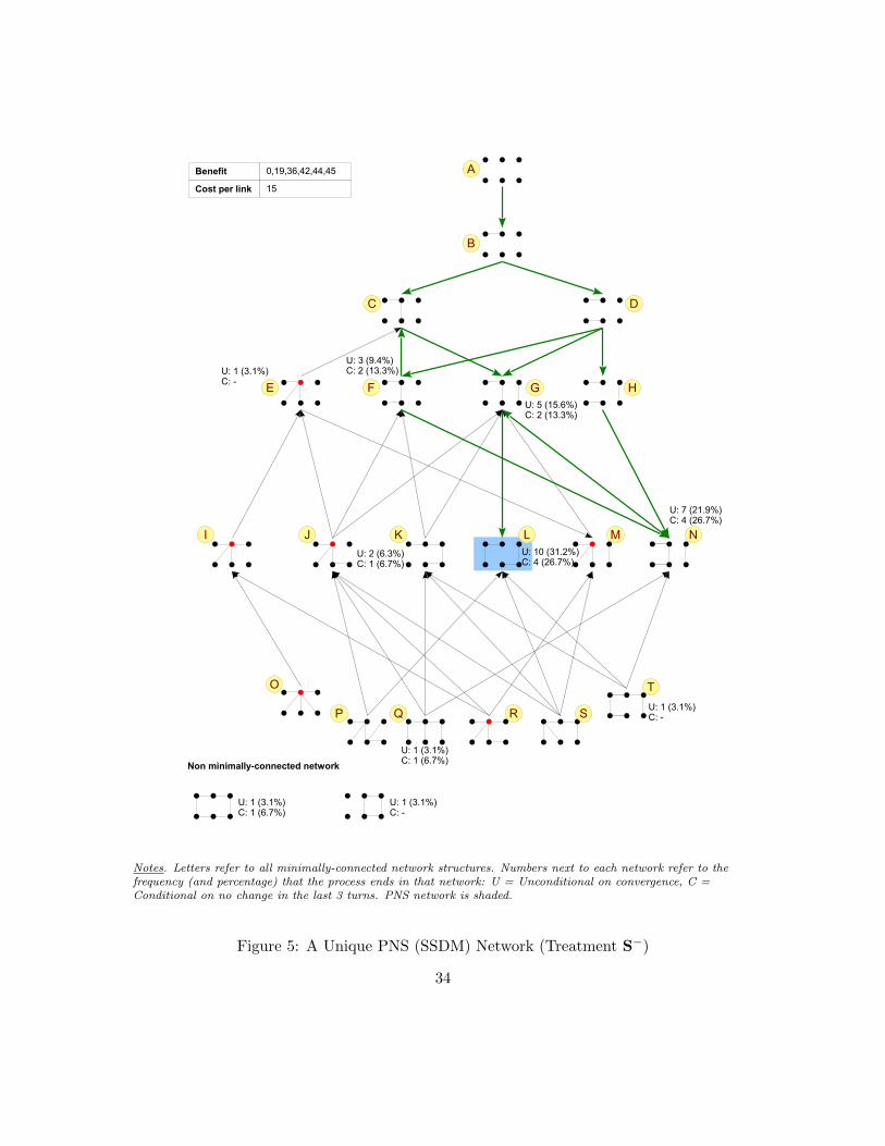
MLKI

N

Non minimally-connected network

J

A

B

T

SRQP

O

HGFE

DC

Benefit 0,19,36,42,44,45

Cost per link 15

U: 1 (3.1%)C: -

U: 3 (9.4%)C: 2 (13.3%)

U: 5 (15.6%)C: 2 (13.3%)

U: 2 (6.3%)C: 1 (6.7%)

U: 10 (31.2%)C: 4 (26.7%)

U: 7 (21.9%)C: 4 (26.7%)

U: 1 (3.1%)C: 1 (6.7%)

U: 1 (3.1%)C: -

U: 1 (3.1%)C: 1 (6.7%)

U: 1 (3.1%)C: -

Notes. Letters refer to all minimally-connected network structures. Numbers next to each network refer to thefrequency (and percentage) that the process ends in that network: U = Unconditional on convergence, C =Conditional on no change in the last 3 turns. PNS network is shaded.

Figure 5: A Unique PNS (SSDM) Network (Treatment S−)

34

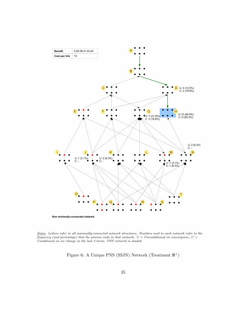
MLKI

N

Non minimally-connected network

J

A

B

T

SRQP

O

HGFE

DC

Benefit 0,29,36,41,43,44

Cost per link 15

U: 4 (12.5%)C: 3 (18.8%)

U: 7 (21.9%)C: 3 (18.8%)

U: 2 (6.3%)C: -

U:15 (46.9%)C: 9 (56.3%)

U: 1 (3.1%)C: 1 (6.3%)

U: 2 (6.3%)C: -

U: 1 (3.1%)C: -

Notes. Letters refer to all minimally-connected network structures. Numbers next to each network refer to thefrequency (and percentage) that the process ends in that network: U = Unconditional on convergence, C =Conditional on no change in the last 3 turns. PNS network is shaded.

Figure 6: A Unique PNS (SSJN) Network (Treatment S+)

35

References

Ai, Chunrong and Edward C. Norton, “Interaction terms in logit and probit models,”

Economics Letters, July 2003, 80, 123–129.

Bala, Venkatesh and Sanjeev Goyal, “A Noncooperative Model of Network Forma-

tion,” Econometrica, September 2000, 68 (5), 1181–1229.

Berman, Eli, “Sect, Subsidy, and Sacrifice: An Economist’s View of Ultra-Orthodox

Jews,” Quarterly Journal of Economics, August 2000, 115, 905–953.

Berninghaus, Siegfried K., Karl-Martin Ehrhart, and Marion Ott, “A network

experiment in continuous time: The influence of link costs,” Experimental Economics,

September 2006, 9 (3), 237–251.

, , , and Bodo Vogt, “Evolution of networks—an experimental analysis,” Journal

of Evolutionary Economics, January 2007, 17 (3), 317–347.

Bloch, Francis and Matthew Jackson, “Definitions of equilibrium in network forma-

tion games,” International Journal of Game Theory, October 2006, 34 (3), 305–318.

Boucher, Vincent and Ismael Mourifie, “My Friend Far Far Away: Asymptotic Prop-

erties of Pairwise Stable Networks,” September 2013.

Bramoulle, Y. and R. Kranton, “Risk-sharing networks,” Journal of Economic Behav-

ior & Organization, 2007, 64 (3-4), 275–294.

Burger, Martijn J. and Vincent Buskens, “Social context and network formation:

An experimental study,” Social Networks, January 2009, 31 (1), 63–75.

Cagno, Daniela Di and Emanuela Sciubba, “The Determinants of Individual Be-

haviour in Network Formation: Some Experimental Evidence,” in Mohammed Abdel-

laoui, John D. Hey, W. Leinfellner, G. Eberlein, and S. H. Tijs, eds., Advances in Decision

Making Under Risk and Uncertainty, Vol. 42 of Theory and Decision Library, Springer

Berlin Heidelberg, 2008, pp. 219–241.

Caldara, Michael and Michael McBride, “An experimental study of network forma-

tion with limited observation,” Unpublished manuscript, July 2015.

Callander, S. and C. R. Plott, “Principles of network development and evolution: An

experimental study,” Journal of Public Economics, 2005, 89 (8), 1469–1495.

36

Candelo, Natalia, Sherry Forbes, Susanne Martin, Michael McBride, and Blake

Allison, “Endogenous Formation of Dark Networks: Theory and Experiment,” 2014.

Charness, Gary, Francesco Feri, Miguel A. Melendez-Jimenez, and Matthias

Sutter, “Experimental Games on Networks: Underpinnings of Behavior and Equilibrium

Selection,” Econometrica, September 2014, 82 (5), 1615–1670.

Chen, Yan and Tayfun Sonmez, “School choice: an experimental study,” Journal of

Economic Theory, March 2006, 127 (1), 202–231.

Comola, Margherita and Marcel Fafchamps, “An Experimental Study of Decentral-

ized Link Formation with Competition,” Technical Report w21758, National Bureau of

Economic Research, Cambridge, MA November 2015.

Conte, Anna, Daniela T. Di Cagno, and Emanuela Sciubba, “Behavioral Patterns

in Social Networks,” Economic Inquiry, April 2015, 53 (2), 1331–1349.

Deck, Cary and Cathleen Johnson, “Link bidding in laboratory networks,” Review

Economic Design, April 2004, 8 (4).

Dutta, Bhaskar and Suresh Mutuswami, “Stable Networks,” Journal of Economic

Theory, October 1997, 76 (2), 322–344.

Echenique, Federico, Alistair J. Wilson, and Leeat Yariv, “Clearinghouses for

Two-Sided Matching: An Experimental Study,” Quantitative Economics, forthcoming.

and Leeat Yariv, “An Experimental Study of Decentralized Matching,” 2013.

Falk, Armin and Michael Kosfeld, “It’s all about Connections: Evidence on Network

Formation,” Review of Network Economics, January 2012, 11 (3).

Fatas, Enrique, Miguel Melendez-Jimenez, and Hector Solaz, “An experimental

analysis of team production in networks,” Experimental Economics, 2010, 13 (4), 399–

411.

Fraley, Chris, Adrian E. Raftery, T.B. Murphy, and L Scrucca, “mclust Version 4

for R: Normal Mixture Modeling for Model-Based Clustering, Classification, and Density

Estimation,” Technical Report 597, Department of Statistics, University of Washington

2012.

and , “Model-Based Clustering, Discriminant Analysis, and Density Estimation,”

Journal of the American Statistical Association, June 2002, 97 (458), 611–631.

37

Gale, D. and L. S. Shapley, “College Admissions and the Stability of Marriage,” The

American Mathematical Monthly, January 1962, 69 (1), 9.

Goeree, Jacob K., Arno Riedl, and Aljaz Ule, “In search of stars: Network formation

among heterogeneous agents,” Games and Economic Behavior, November 2009, 67 (2),

445–466.

Greene, William, “The behaviour of the maximum likelihood estimator of limited de-

pendent variable models in the presence of fixed effects,” Econometrics Journal, 2004, 7

(1), 98–119.

, “Testing hypotheses about interaction terms in nonlinear models,” Economics Letters,

May 2010, 107 (2), 291–296.

Jackson, Matthew O., Social and economic networks, Princeton NJ: Princeton Univer-

sity Press, 2008.

, “Networks in the Understanding of Economic Behaviors,” Journal of Economic Per-

spectives, November 2014, 28 (4), 3–22.

and Alison Watts, “The Evolution of Social and Economic Networks,” Journal of

Economic Theory, October 2002, 106 (2), 265–295.

and Anne van den Nouweland, “Strongly stable networks,” Games and Economic

Behavior, May 2005, 51 (2), 420–444.

and Asher Wolinsky, “A Strategic Model of Social and Economic Networks,” Journal

of Economic Theory, October 1996, 71 (1), 44–74.

Kirchsteiger, Georg, Marco Mantovani, Ana Mauleon, and Vincent Vannetel-

bosch, “Limited farsightedness in network formation,” Discussion Paper 8263, CORE,

Belgium May 2013.

McKelvey, Richard and Thomas Palfrey, “Quantal Response Equilibria for Normal

Form Games,” Games and Economic Behavior, July 1995, 10 (1), 6–38.

Myerson, Roger B, Game theory: analysis of conflict, Cambridge, Mass.: Harvard Uni-

versity Press, 1991.

Pantz, Katinka, The strategic formation of social networks : experimental evidence,

Aachen: Shaker, 2006.

38

Sheng, Shuyang, “A Structural Econometric Analysis of Network Formation Games,”

June 2014.

Teteryatnikova, Mariya and James Tremewan, “Stability of Networks with Con-

tinuous Stream of Payoffs: A Theory and Experiment,” Unpublished manuscript April

2015.

Watts, Alison, “A Dynamic Model of Network Formation,” Games and Economic Be-

havior, February 2001, 34 (2), 331–341.

39

APPENDIX (for online publication)

A Treatment M: Multiplicity of PNS networks

With Treatment M, we examine a game with multiple stable networks. We use the multi-

plicity of stable networks to examine whether subjects play some form of forward-looking

behavior. A feature of the treatment is that subjects need to deviate from myopic ratio-

nality – and take the risk of incurring negative payoffs – in order to reach the (Pareto-

dominant) stable network with strictly positive payoffs. This situation mimics the problem

of network formation in scale economies, where the first few links have negative net benefits

to the first adopters.

Figure A.1 depicts the payoff structure, improving paths, and stable networks in Treat-

ment M. The treatment has four pairwise stable networks. Two of these are PNS networks

{A,K}, where {A} is stochastically stable while {K} is SSDM. The remaining two ({I, J})are not Nash stable. The payoffs of the SSDM network {K} Pareto-dominate those in the

empty PNS network {A}. The analysis is relegated to the appendix because our original

intention was to build a network formation game with exactly two pairwise stable networks.

Due to a mistake in programming, the game has four instead, which interferes with the

analysis of the data and the interpretation of results. For transparency but also because

the basic results are interesting, we summarize below the main findings.

The setup provides a direct test of the assumption of myopic rationality in network

formation. To illustrate, the movement from network {A} to {B} requires that linking

subjects be willing to risk receiving negative payoffs. If subjects primarily make myopic

rational choices, then the network will be “stable” at A. However, if enough subjects are

willing to deviate from the myopic rational strategy, they may reach the Pareto-dominant

SSDM network {K}.

The set of deviations required to reach network {K} from {A} is non-trivial. Define the

resistance between networks g and g′ as the minimum number of mutations (i.e., deviations

from an improving path) necessary to evolve from g to g′ (Jackson and Watts, 2002). In

Treatment M, the resistance between the starting network and the SSDM network equals

to four.

We find evidence of strategic (forward-looking) behavior among the experimental sub-

jects. At the network level, despite the non-trivial resistance, the dynamic link formation

process did lead by and large to the SSDM network. Indeed, 44 percent (unconditional

on convergence) and 55 percent (conditional on convergence) of matches in Treatment M

ended in the SSDM network. By contrast, no match ended in the empty, stochastically-

A-1

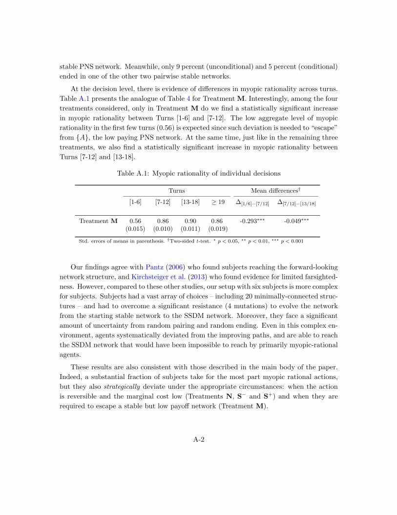
stable PNS network. Meanwhile, only 9 percent (unconditional) and 5 percent (conditional)

ended in one of the other two pairwise stable networks.

At the decision level, there is evidence of differences in myopic rationality across turns.

Table A.1 presents the analogue of Table 4 for Treatment M. Interestingly, among the four

treatments considered, only in Treatment M do we find a statistically significant increase

in myopic rationality between Turns [1-6] and [7-12]. The low aggregate level of myopic

rationality in the first few turns (0.56) is expected since such deviation is needed to “escape”

from {A}, the low paying PNS network. At the same time, just like in the remaining three

treatments, we also find a statistically significant increase in myopic rationality between

Turns [7-12] and [13-18].

Table A.1: Myopic rationality of individual decisions

Turns Mean differences†

[1-6] [7-12] [13-18] ≥ 19 ∆[1/6]−[7/12] ∆[7/12]−[13/18]

Treatment M 0.56 0.86 0.90 0.86 -0.293∗∗∗ -0.049∗∗∗

(0.015) (0.010) (0.011) (0.019)

Std. errors of means in parenthesis. †Two-sided t-test. ∗ p < 0.05, ∗∗ p < 0.01, ∗∗∗ p < 0.001

Our findings agree with Pantz (2006) who found subjects reaching the forward-looking

network structure, and Kirchsteiger et al. (2013) who found evidence for limited farsighted-

ness. However, compared to these other studies, our setup with six subjects is more complex

for subjects. Subjects had a vast array of choices – including 20 minimally-connected struc-

tures – and had to overcome a significant resistance (4 mutations) to evolve the network

from the starting stable network to the SSDM network. Moreover, they face a significant

amount of uncertainty from random pairing and random ending. Even in this complex en-

vironment, agents systematically deviated from the improving paths, and are able to reach

the SSDM network that would have been impossible to reach by primarily myopic-rational

agents.

These results are also consistent with those described in the main body of the paper.

Indeed, a substantial fraction of subjects take for the most part myopic rational actions,

but they also strategically deviate under the appropriate circumstances: when the action

is reversible and the marginal cost low (Treatments N, S− and S+) and when they are

required to escape a stable but low payoff network (Treatment M).

A-2

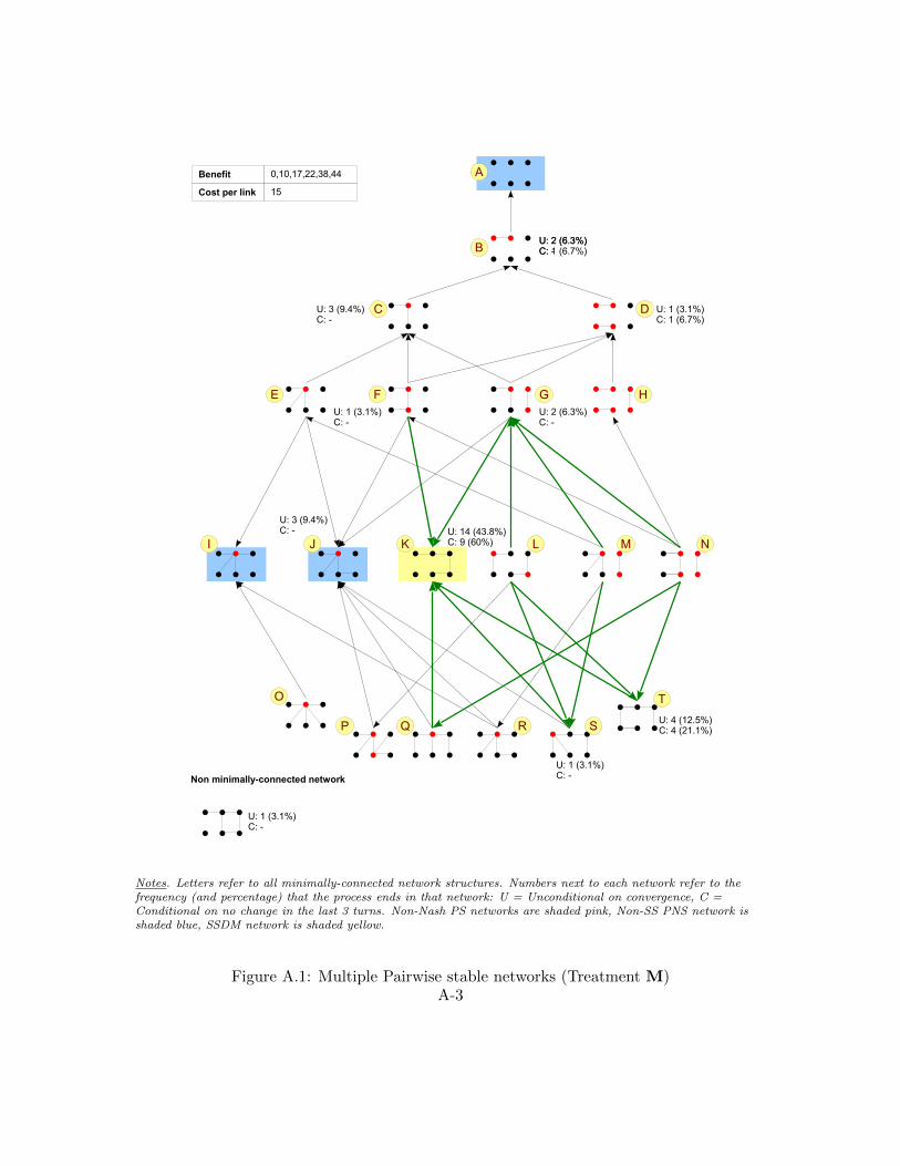
MLI

N

K

Non minimally-connected network

J

A

B

T

SRQP

O

HGFE

DC

Benefit 0,10,17,22,38,44

Cost per link 15

U: 2 (6.3%)C: -

U: 2 (6.3%)C: -

U: 3 (9.4%)C: -

U: 2 (6.3%)C: 1 (6.7%)

U: 1 (3.1%)C: 1 (6.7%)

U: 1 (3.1%)C: -

U: 1 (3.1%)C: -

U: 1 (3.1%)C: -

U: 4 (12.5%)C: 4 (21.1%)

U: 14 (43.8%)C: 9 (60%)

U: 3 (9.4%)C: -

Notes. Letters refer to all minimally-connected network structures. Numbers next to each network refer to thefrequency (and percentage) that the process ends in that network: U = Unconditional on convergence, C =Conditional on no change in the last 3 turns. Non-Nash PS networks are shaded pink, Non-SS PNS network isshaded blue, SSDM network is shaded yellow.

Figure A.1: Multiple Pairwise stable networks (Treatment M)A-3

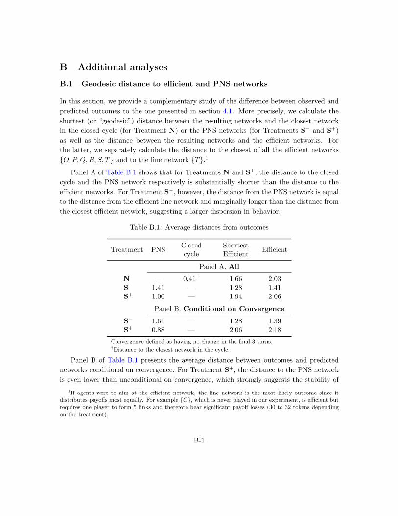
B Additional analyses

B.1 Geodesic distance to efficient and PNS networks

In this section, we provide a complementary study of the difference between observed and

predicted outcomes to the one presented in section 4.1. More precisely, we calculate the

shortest (or “geodesic”) distance between the resulting networks and the closest network

in the closed cycle (for Treatment N) or the PNS networks (for Treatments S− and S+)

as well as the distance between the resulting networks and the efficient networks. For

the latter, we separately calculate the distance to the closest of all the efficient networks

{O,P,Q,R, S, T} and to the line network {T}.1

Panel A of Table B.1 shows that for Treatments N and S+, the distance to the closed

cycle and the PNS network respectively is substantially shorter than the distance to the

efficient networks. For Treatment S−, however, the distance from the PNS network is equal

to the distance from the efficient line network and marginally longer than the distance from

the closest efficient network, suggesting a larger dispersion in behavior.

Table B.1: Average distances from outcomes

Treatment PNSClosedcycle

ShortestEfficient

Efficient

Panel A. All

N — 0.41 † 1.66 2.03S− 1.41 — 1.28 1.41S+ 1.00 — 1.94 2.06

Panel B. Conditional on Convergence

S− 1.61 — 1.28 1.39S+ 0.88 — 2.06 2.18

Convergence defined as having no change in the final 3 turns.†Distance to the closest network in the cycle.

Panel B of Table B.1 presents the average distance between outcomes and predicted

networks conditional on convergence. For Treatment S+, the distance to the PNS network

is even lower than unconditional on convergence, which strongly suggests the stability of

1If agents were to aim at the efficient network, the line network is the most likely outcome since itdistributes payoffs most equally. For example {O}, which is never played in our experiment, is efficient butrequires one player to form 5 links and therefore bear significant payoff losses (30 to 32 tokens dependingon the treatment).

B-1

the SSJN network. In contrast, the distance from the convergent network to the efficient

network is lower than to the PNS network in Treatment S−. Results from Panels A and B

come from the fact that most of the network outcomes in Treatment S−, both conditional

and unconditional on convergence, are split almost equally between the PNS network {L}and network {N}. Since the distance between these two networks is two and both of them

are at a distance of one to the efficient networks, the distance from the stable network and

the efficient networks are similar. It is difficult to infer from the outcomes alone where

the formation processes is leading toward. Our analysis of individual decisions (Result 2)

provides a plausible explanation for these findings.

B.2 Myopic rationality by treatment and decision problem

Figure B.1 further illustrates the results in Panels B and C of Table 4. We plot for each

treatment the proportion of myopic rational behavior across turns when passing is rational

(B1) and when acting is rational (B2). In all treatments, players maintain more links in

all turns than would be observed if they played myopically rational all the time. The gap

is bigger and the variation larger for decisions where acting is myopic rational (figures on

the right), although the difference narrows as the match nears its end.

B.3 Pooled FE LPM on probability of myopic rational choices

To test whether there is a structural break in behavior at Turn 12, we implemented a test

of pooling that is estimated using the fixed-effects LPM. For each treatment, we estimated

models based on Equations 2 and 3, but interacted each of the variables with an indicator

variable of whether an observation comes after Turn 12, 1(turn > 12).

Table B.2 presents the fixed effects pooled LPM to investigate if there is a difference

in myopic rational choices before and after Turn 12. To test whether there are structural

breaks in the variables, we conducted a joint test of all interacted variables. The p-value of

this test is presented at the bottom of the table. For all treatments and specifications, the

null hypothesis of no structural break at Turn 12 is rejected at the 5 percent significance

level.

B.4 Effect of experience

As described in Section 3, each subject played each treatment twice. We use this to examine

whether subjects altered their behavior the second time they encountered a treatment. We

implemented a test of structural break akin to the pooling test described in Section B.3.

B-2

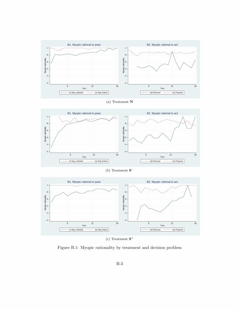
1.8

.6.4

.20

Myo

pic

ratio

nalit

y

6 12 18Turn

(i) Stay unlinked (ii) Stay linked

B1. Myopic rational to pass

1.8

.6.4

.20

Myo

pic

ratio

nalit

y

6 12 18Turn

(iii) Remove (iv) Propose

B2. Myopic rational to act

(a) Treatment N

1.8

.6.4

.20

Myo

pic

ratio

nalit

y

6 12 18Turn

(i) Stay unlinked (ii) Stay linked

B1. Myopic rational to pass

1.8

.6.4

.20

Myo

pic

ratio

nalit

y

6 12 18Turn

(iii) Remove (iv) Propose

B2. Myopic rational to act

(b) Treatment S−

1.8

.6.4

.20

Myo

pic

ratio

nalit

y

6 12 18Turn

(i) Stay unlinked (ii) Stay linked

B1. Myopic rational to pass

1.8

.6.4

.20

Myo

pic

ratio

nalit

y

6 12 18Turn

(iii) Remove (iv) Propose

B2. Myopic rational to act

(c) Treatment S+

Figure B.1: Myopic rationality by treatment and decision problem

B-3

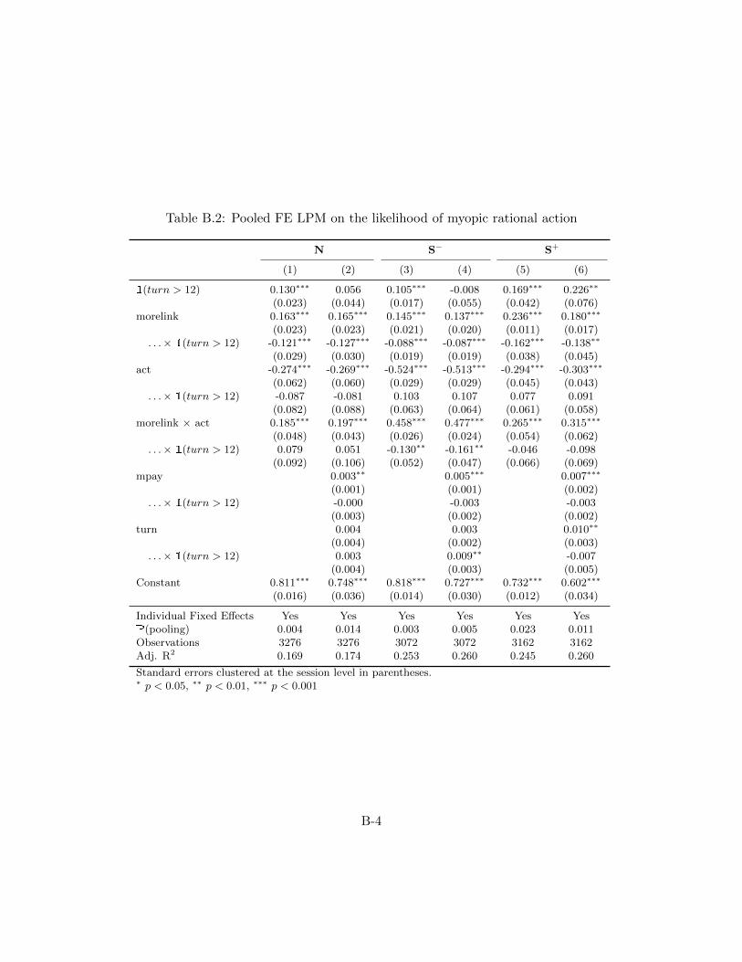
Table B.2: Pooled FE LPM on the likelihood of myopic rational action

N S− S+

(1) (2) (3) (4) (5) (6)

1(turn > 12) 0.130∗∗∗ 0.056 0.105∗∗∗ -0.008 0.169∗∗∗ 0.226∗∗

(0.023) (0.044) (0.017) (0.055) (0.042) (0.076)morelink 0.163∗∗∗ 0.165∗∗∗ 0.145∗∗∗ 0.137∗∗∗ 0.236∗∗∗ 0.180∗∗∗

(0.023) (0.023) (0.021) (0.020) (0.011) (0.017). . .× 1(turn > 12) -0.121∗∗∗ -0.127∗∗∗ -0.088∗∗∗ -0.087∗∗∗ -0.162∗∗∗ -0.138∗∗

(0.029) (0.030) (0.019) (0.019) (0.038) (0.045)act -0.274∗∗∗ -0.269∗∗∗ -0.524∗∗∗ -0.513∗∗∗ -0.294∗∗∗ -0.303∗∗∗

(0.062) (0.060) (0.029) (0.029) (0.045) (0.043). . .× 1(turn > 12) -0.087 -0.081 0.103 0.107 0.077 0.091

(0.082) (0.088) (0.063) (0.064) (0.061) (0.058)morelink × act 0.185∗∗∗ 0.197∗∗∗ 0.458∗∗∗ 0.477∗∗∗ 0.265∗∗∗ 0.315∗∗∗

(0.048) (0.043) (0.026) (0.024) (0.054) (0.062). . .× 1(turn > 12) 0.079 0.051 -0.130∗∗ -0.161∗∗ -0.046 -0.098

(0.092) (0.106) (0.052) (0.047) (0.066) (0.069)mpay 0.003∗∗ 0.005∗∗∗ 0.007∗∗∗

(0.001) (0.001) (0.002). . .× 1(turn > 12) -0.000 -0.003 -0.003

(0.003) (0.002) (0.002)turn 0.004 0.003 0.010∗∗

(0.004) (0.002) (0.003). . .× 1(turn > 12) 0.003 0.009∗∗ -0.007

(0.004) (0.003) (0.005)Constant 0.811∗∗∗ 0.748∗∗∗ 0.818∗∗∗ 0.727∗∗∗ 0.732∗∗∗ 0.602∗∗∗

(0.016) (0.036) (0.014) (0.030) (0.012) (0.034)

Individual Fixed Effects Yes Yes Yes Yes Yes YesP(pooling) 0.004 0.014 0.003 0.005 0.023 0.011Observations 3276 3276 3072 3072 3162 3162Adj. R2 0.169 0.174 0.253 0.260 0.245 0.260

Standard errors clustered at the session level in parentheses.∗ p < 0.05, ∗∗ p < 0.01, ∗∗∗ p < 0.001

B-4

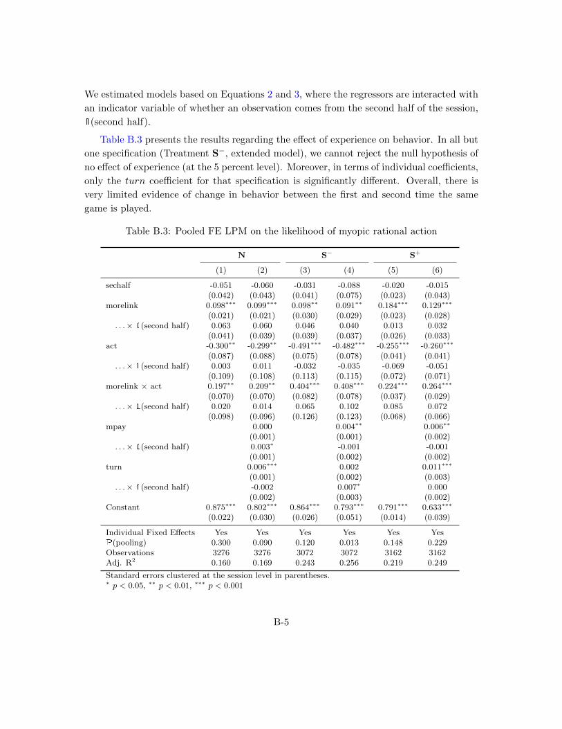
We estimated models based on Equations 2 and 3, where the regressors are interacted with

an indicator variable of whether an observation comes from the second half of the session,

1(second half).

Table B.3 presents the results regarding the effect of experience on behavior. In all but

one specification (Treatment S−, extended model), we cannot reject the null hypothesis of

no effect of experience (at the 5 percent level). Moreover, in terms of individual coefficients,

only the turn coefficient for that specification is significantly different. Overall, there is

very limited evidence of change in behavior between the first and second time the same

game is played.

Table B.3: Pooled FE LPM on the likelihood of myopic rational action

N S− S+

(1) (2) (3) (4) (5) (6)

sechalf -0.051 -0.060 -0.031 -0.088 -0.020 -0.015(0.042) (0.043) (0.041) (0.075) (0.023) (0.043)

morelink 0.098∗∗∗ 0.099∗∗∗ 0.098∗∗ 0.091∗∗ 0.184∗∗∗ 0.129∗∗∗

(0.021) (0.021) (0.030) (0.029) (0.023) (0.028). . .× 1(second half) 0.063 0.060 0.046 0.040 0.013 0.032

(0.041) (0.039) (0.039) (0.037) (0.026) (0.033)act -0.300∗∗ -0.299∗∗ -0.491∗∗∗ -0.482∗∗∗ -0.255∗∗∗ -0.260∗∗∗

(0.087) (0.088) (0.075) (0.078) (0.041) (0.041). . .× 1(second half) 0.003 0.011 -0.032 -0.035 -0.069 -0.051

(0.109) (0.108) (0.113) (0.115) (0.072) (0.071)morelink × act 0.197∗∗ 0.209∗∗ 0.404∗∗∗ 0.408∗∗∗ 0.224∗∗∗ 0.264∗∗∗

(0.070) (0.070) (0.082) (0.078) (0.037) (0.029). . .× 1(second half) 0.020 0.014 0.065 0.102 0.085 0.072

(0.098) (0.096) (0.126) (0.123) (0.068) (0.066)mpay 0.000 0.004∗∗ 0.006∗∗

(0.001) (0.001) (0.002). . .× 1(second half) 0.003∗ -0.001 -0.001

(0.001) (0.002) (0.002)turn 0.006∗∗∗ 0.002 0.011∗∗∗

(0.001) (0.002) (0.003). . .× 1(second half) -0.002 0.007∗ 0.000

(0.002) (0.003) (0.002)Constant 0.875∗∗∗ 0.802∗∗∗ 0.864∗∗∗ 0.793∗∗∗ 0.791∗∗∗ 0.633∗∗∗

(0.022) (0.030) (0.026) (0.051) (0.014) (0.039)

Individual Fixed Effects Yes Yes Yes Yes Yes YesP(pooling) 0.300 0.090 0.120 0.013 0.148 0.229Observations 3276 3276 3072 3072 3162 3162Adj. R2 0.160 0.169 0.243 0.256 0.219 0.249

Standard errors clustered at the session level in parentheses.∗ p < 0.05, ∗∗ p < 0.01, ∗∗∗ p < 0.001

B-5

C Instructions

Welcome. This is an experiment on individual decision making in groups, and you will be

paid for your participation in cash at the end of the experiment. The entire experiment

will take place through computer terminals, and all interactions between participants will

take place through the computers. You will remain anonymous to me and to all the other

participants during the entire experiment; the only person who will know your identity is

the Lab Manager who is responsible for paying you in the end. Moreover, it is important

that you do not talk or in any way try to communicate with other participants during the

experiment.

We will start with a brief instruction period. During the instruction period, you will be

given a complete description of the experiment and will be shown how to use the computers.

You must take a quiz after the instruction period, so it is important that you listen carefully.

If you have any questions during the instruction period, raise your hand and your question

will be answered so everyone can hear. If any difficulties arise after the experiment has

begun, raise your hand, and an experimenter will come and assist you. Please note that

you are not being deceived and you will not be deceived: everything I tell you is true.

Your earnings during the experiment are denominated in tokens. Depending on your

decisions, you can earn more tokens or lose some tokens. At the end of the experiment,

we will count the number of tokens you have earned in all of the matches and you will

receive $1.00 for every 4 tokens. You will be paid this amount plus the show-up fee of $5.

Different participants may earn different amounts. Everyone will be paid in private and

you are under no obligation to tell others how much you earned.

The experiment will consist of 8 matches. In each match, you will be put in a group with

5 other participants in the experiment. Since there are 12 participants in today’s session,

there will be 2 groups in each match. You are not told the identity of the participants in

your group. Your payoff in each match depends only on your decisions, the decisions of the

other 5 participants in your group and on chance. What happens in the other group has

no effect on your payoff and vice versa. Your decisions are not revealed to participants in

the other group.

We will now explain how each match proceeds. At the beginning of the match, the

computer randomly assigns each of you to a group consisting of 6 participants. Next, the

computer randomly assigns with equal probability a role to each of the participants as

“Subject 1”, “Subject 2” and so on up to “Subject 6”. Then, the match begins.

Each match consists of several turns. At the beginning of each turn, the computer

randomly pairs all subjects within each group with one another. We shall call the subject

C-1

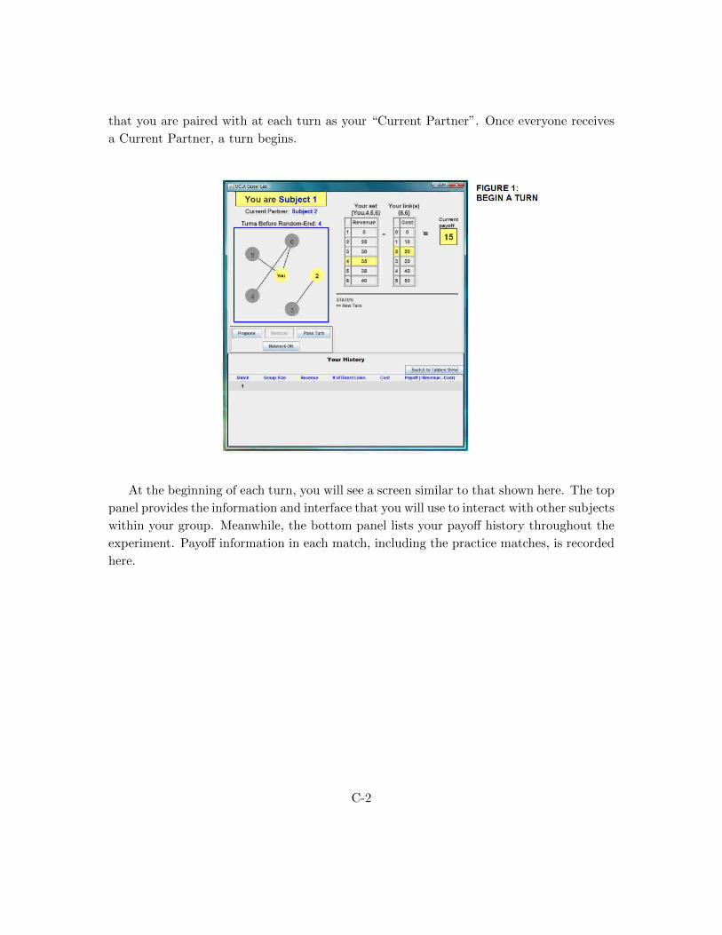
that you are paired with at each turn as your “Current Partner”. Once everyone receives

a Current Partner, a turn begins.

At the beginning of each turn, you will see a screen similar to that shown here. The top

panel provides the information and interface that you will use to interact with other subjects

within your group. Meanwhile, the bottom panel lists your payoff history throughout the

experiment. Payoff information in each match, including the practice matches, is recorded

here.

C-2

This is the top panel. On the top-left is your role in this match. In this example, you

are Subject 1. The computer also informs you of your Current Partner at each turn. In

this turn, your Current Partner is Subject 2.

In the middle of the left panel, you will see a network representation of the connections

between all subjects in your group. Other subjects in your group are represented by nodes

with their role ID numbers. Meanwhile, you are always represented by the center node

labeled “YOU”. In each turn, the node for your Current Partner is colored YELLOW

unlike the rest of the subjects. From the color, you can see here that your Current Partner

is Subject 2.

The lines connecting the nodes represent the links between subjects in your group.

Everyone in your group sees the same sets of links. In this example, you have direct links

to Subjects 5 and 6. Through Subject 6, your are also indirectly connected with Subject 4.

Subjects who are either directly or indirectly connected belong in the same “Set”. In this

example, there are two sets. The first consists of You, Subjects 4, 5, and 6. The second

set consists of Subjects 2 and 3.

At each turn, the joint actions of you and your current partner affect how the two of

you are linked. You take actions by clicking one of the action buttons below the network

representation. Through your actions, you can either propose a link, remove a link, or

maintain how you are connected with your partner.

C-3

In this first example, since you are not linked to Subject 2, only three actions are

available: “Propose”, “Pass Turn”, and “Network OK”. The “Remove” button is not

active. Clicking “Propose” lets the computer know that you would like to propose a link

with your Current Partner. If your partner does the same, the computer will create a link

between you and your partner. Otherwise, no link will be created. In other words, a link

is created if and only if BOTH partners propose a link to each other.

If you don't want to link with your Current Partner, you can either click “Pass Turn”

or “Network OK”. In either case, a link will not be created. However, notice the difference

between the two actions. When you pass a turn, you tell the computer that you want to

keep the way you are linked with your current partner in this turn. However, you may still

want to change how you are linked with some of the other subjects. So, your buttons will

remain active in the next turn

Meanwhile, if you choose “Network OK”, you tell the computer that as long as the

network doesn't change, you are happy with the way you are linked with everyone in your

group. Therefore, if you click “Network OK”, you won't need to take further actions until

the network changes. Your buttons will therefore be inactive. However, these buttons will

immediately become active once the decisions of other pairs either break or make a link.

If all active subjects choose “Network OK” in the same turn, then the match ends.

The turn ends once everyone in your group has taken an action. The computer then

begins a new turn, and you will be randomly assigned a new Current Partner. Please

note that since pairs are selected randomly, you may be paired with the same partner in

consecutive turns.

C-4

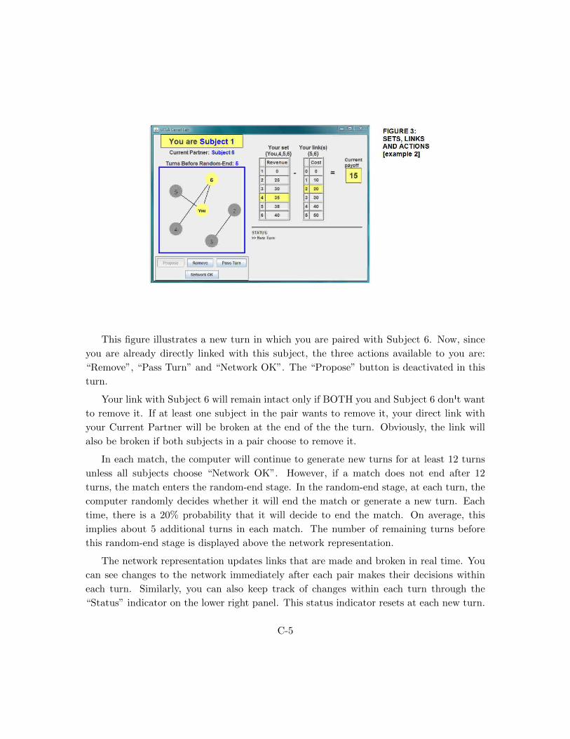
This figure illustrates a new turn in which you are paired with Subject 6. Now, since

you are already directly linked with this subject, the three actions available to you are:

“Remove”, “Pass Turn” and “Network OK”. The “Propose” button is deactivated in this

turn.

Your link with Subject 6 will remain intact only if BOTH you and Subject 6 don't want

to remove it. If at least one subject in the pair wants to remove it, your direct link with

your Current Partner will be broken at the end of the the turn. Obviously, the link will

also be broken if both subjects in a pair choose to remove it.

In each match, the computer will continue to generate new turns for at least 12 turns

unless all subjects choose “Network OK”. However, if a match does not end after 12

turns, the match enters the random-end stage. In the random-end stage, at each turn, the

computer randomly decides whether it will end the match or generate a new turn. Each

time, there is a 20% probability that it will decide to end the match. On average, this

implies about 5 additional turns in each match. The number of remaining turns before

this random-end stage is displayed above the network representation.

The network representation updates links that are made and broken in real time. You

can see changes to the network immediately after each pair makes their decisions within

each turn. Similarly, you can also keep track of changes within each turn through the

“Status” indicator on the lower right panel. This status indicator resets at each new turn.

C-5

We will next discuss about the payoff. Your payoff depends on the size of your set and

the number of direct links at the end of the match. Your set size, which is the number of

subjects who are either directly or indirectly connected to you, determines your revenue.

Meanwhile, your cost is determined by the number of direct links you have.

The right panel provides you with all of the information necessary to calculate your

payoff. The table on the left gives you the revenue schedule for different set sizes. Above

it, you can see the list of subjects in your set. In this example, your set consists of You

and Subjects 4, 5, and 6. Therefore, as part of a set of size 4, your revenue is 35.

Next to the revenue table is the cost schedule for different numbers of direct links.

Each direct link incurs a constant cost. In this particular example, the cost for each link

is 10 and, therefore, the total cost is 10 times the number of subjects with whom you are

directly linked. Above that table, you can see that you are directly linked to Subjects 5

and 6. Since you have two direct links, the current total cost is 20 tokens.

Your current revenue and cost at any stage of the game are highlighted in YELLOW.

They are updated in real time as the actions of subjects make and break links within each

turn. The rightmost box entitled “Current Payoff” calculates your payoff at each stage of

the game. The current payoff is simply the revenue minus cost, which in this case is 15.

This payoff information is also updated in real time. Note that the revenue and cost tables

may change from match to match.

C-6

This figure illustrates what you will see at the end of a match. Below the status

indicator, you will see your payoff for this match. At the end of the match, please click

“Continue to the Next Match”. In each new match, you will be randomly assigned to a

new group. A new match will begin only after all groups have completed their matches.

This continues for 8 matches, after which the experiment ends.

At the end of the final match in the experiment, you will see the following screen.

This final screen tells you the total payoff that you will receive for this experiment.

When you see this screen, don't click OK until you have written down your total payoff

on the payoff sheet provided. After you have written down your total payoff, click OK to

conclude the session. (*)

The following slides summarize the rules of the experiment:

C-7

We will now begin the Practice session and go through two practice matches to famil-

iarize you with the computer interface and the procedures. During these practice matches,

C-8

please do not hit any keys until you are asked to. Remember, you are not paid for these

matches. At the end of the practice matches you will have to answer some review questions.

Throughout the session, pay attention to the network representation display and status

indicators. Also, notice the movements of the yellow highlights on your Revenue and Cost

tables, as well as updates to your Current Payoff.

[START GAME]

You have just received a new turn. First, pay attention to your role. If you are Subject 1,

2, or 3, please click “Propose”. For Subject 1, 2, or 3, notice a link has just been created

between you and your partner if your partner is also Subject 1, 2 or 3.

Now, if you are Subject 4, 5, or 6, please click the “Pass Turn” button. Notice here

that a link is created if and only if BOTH partners propose a link. If only one partner

proposes a link, no link is created.

You have moved to a new turn. We will now see how the “Network OK” action works.

If you are either Subject 5 or 6, please click “Network OK”. For the rest of the group,

please click “Pass Turn”.

You have moved to a new turn. For Subjects 5 or 6, since the network has not changed

after you clicked “Network OK”, all of your buttons are now inactive. Notice that they

will become active following a change in the network.

For others, please check your Current Partner. If your partner is not Subject 5 or 6,

click the “Remove” button if it's active or “Propose” otherwise. For Subjects 5 and 6,

notice how a change in the network activates your buttons.

If you are not Subject 5 or 6 and your buttons are still active, please click “Pass Turn”.

If you are Subject 5 or 6 and your buttons are active, please click “Pass Turn”. Notice

here that if your buttons are inactive due to a “Network OK” action in a previous turn, a

change in the network will immediately activate your buttons. In the following, we will do

the same exercise for Subjects 1 to 4.

You have moved to a new turn. If you are Subject 3 or 4, please click “Network OK”.

For the rest of the group, please click “Pass Turn”.

You have moved to a new turn. Subjects 3 and 4, notice that your buttons are inactive.

If the network changes in this turn, your buttons will become activated.

For all others, check your Current Partner. If your partner is not Subject 3 or 4, click

“Remove” if it's active or click “Propose” otherwise. If you are not Subject 3 or 4 and

C-9

your buttons are still active, click “Pass Turn”. Now, if you are Subject 3 or 4, please click

“Pass Turn”.

You have moved to a new turn. If you are either Subject number 1 or 2, please click

“Network OK”. For the rest, please click “Pass Turn”.

You have moved to a new turn. For Subject 1 or 2, your buttons are now inactive. For

all others, if your Current Partner is not Subject 1 or 2, click the “Remove” button if it's

active, or click “Propose” otherwise. For everyone else who has not taken an action, please

click “Pass Turn”.

You have moved to a new turn. Notice from the message above the network display

that this is the last turn before the random-end stage. During the paid match, you will

have 12 turns before entering this stage. If the match has not ended after 12 turns, the

computer will randomly decide the end of the match.

We will now deliberately end the match. If your buttons are active, please click the

“Network OK” button. This ends the first practice match. The bottom part of your screen

contains a table summarizing the results for all matches you have participated in. This

is called the history screen. It will be filled out as the experiment proceeds. Now click

“Continue to the Next Match”. We will now begin with the second practice match.

[NEXT MATCH]

You are in a new match. Note here that the revenue and cost tables have changed as they

may during the real matches. We'll now examine the behavior of the “Remove” action.

If you are either Subject 2, 4, or 6, please click “Remove”. For Subjects 1, 3, and 5,

please click “Pass Turn”. Hence, notice that a link is broken if at least one of the partners

chooses to remove it.

You have moved to a new turn. Next, we'll see what will happen if the network changes

within the turn in which you click “Network OK”. If you are Subject number 1, 3, or 5,

please click the “Network OK” button. For all others, please click your “Remove” button.

You have moved to a new turn. For Subjects 1, 3, or 5 notice that if in the previous

turn the network changed after you clicked “Network OK”, your action buttons are active

in this turn. If the network did not change after you clicked “Network OK”, your buttons

remain inactive. Now, if you are either Subject 2, 4, or 6, click “Network OK”. For all

C-10

others, if you haven't taken an action in this turn, please click the “Remove” button if it's

active, or “Propose” otherwise.

You have moved to a new turn. Similarly for Subjects 2, 4, and 6, notice that if in

the previous turn the network changed after you clicked “Network OK”, your buttons are

now active. If the network did not change after you clicked “Network OK”, your buttons

are still inactive. If the network changes in the same turn and after you choose “Network

OK”, your buttons stay active in the following turn.

We will now end the match. If your buttons are active, please click “Network OK”.

This ends the second practice match.

*** END OF PRACTICE SESSION ***

The practice matches are over. Please click “Continue to the next match” and complete

the quiz. It has 8 questions in two pages. You will move to the next page once everyone

in your group has completed the questions in that page correctly. On your table, you will

find the screenshots that you will need to answer these questions. Raise your hand if you

have any questions.

[WAIT for everyone to finish the quiz]

Are there any questions before we begin with the paid session? We will now begin with

the 8 paid matches. Please pull out your dividers. If there are any problems or questions

from this point on, raise your hand and an experimenter will come and assist you.

[START MATCH 1]

[After MATCH 8, read:]

This was the last match of the experiment. Now, please write down your ID on the

payment sheet. Your ID is located on top of your physical monitor and it began with

CASSEL. At this point, if you haven't clicked “Continue to the next match”, please do

so. Your total payoff is displayed on your screen. Please record this payoff in the earned

column of your sheet and sign it. Once you have written it down, please click OK.

C-11

Your Total Payoff will be this amount rounded up to the nearest dollar plus the show-up

fee of $5. We will pay each of you in private in the next room. Remember you are under

no obligation to reveal your earnings to the other subjects.

If you are done, please line up behind the yellow line until the lab manager calls you

to be paid. Do not converse with the other subjects or use your cell phone. Thank you for

your cooperation.

C-12