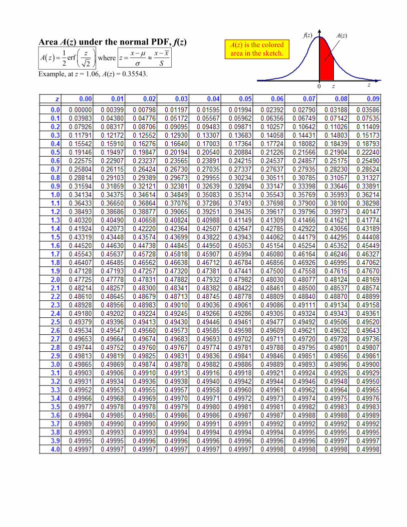
Area A(z) under the normal PDF, f(z)

1

erf2 2

zA z

where

x x xz

S

Example, at z = 1.06, A(z) = 0.35543.

f(z)

z z 0

A(z)

A(z) is the colored

area in the sketch.

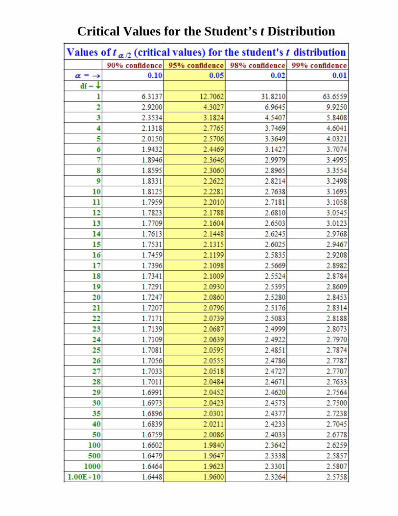
Critical Values for the Student’s t Distribution

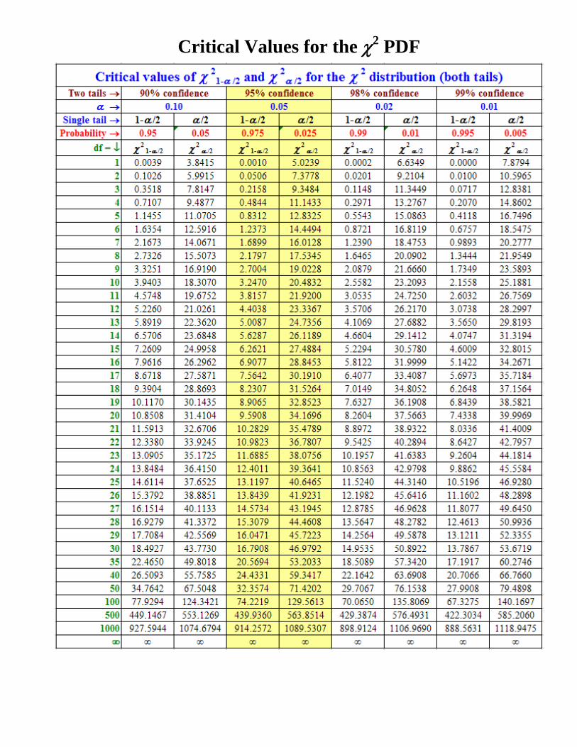
Critical Values for the χ2 PDF

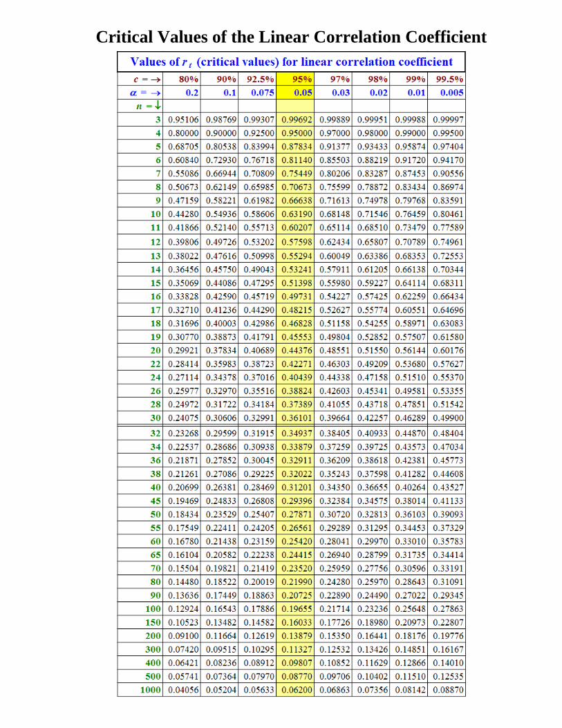
Critical Values of the Linear Correlation Coefficient

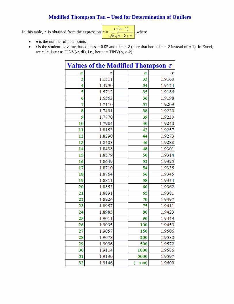
Modified Thompson Tau – Used for Determination of Outliers

In this table, τ is obtained from the expression ( )

2

1

2

t n

n n tτ

⋅ −=

− +, where

• n is the number of data points • t is the student’s t value, based on α = 0.05 and df = n-2 (note that here df = n-2 instead of n-1). In Excel,

we calculate t as TINV(α, df), i.e., here t = TINV(α, n-2)

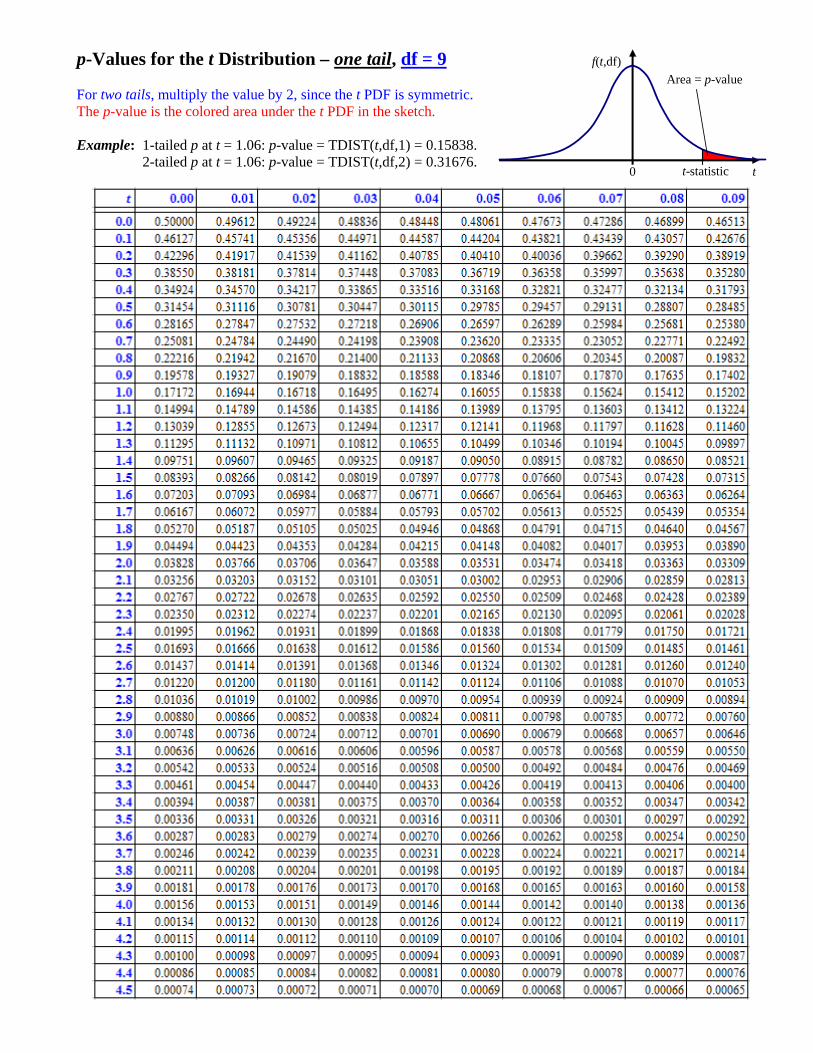
p-Values for the t Distribution – one tail, df = 9 f(t,df)

t t-statistic 0

Area = p-value For two tails, multiply the value by 2, since the t PDF is symmetric. The p-value is the colored area under the t PDF in the sketch. Example: 1-tailed p at t = 1.06: p-value = TDIST(t,df,1) = 0.15838. 2-tailed p at t = 1.06: p-value = TDIST(t,df,2) = 0.31676.

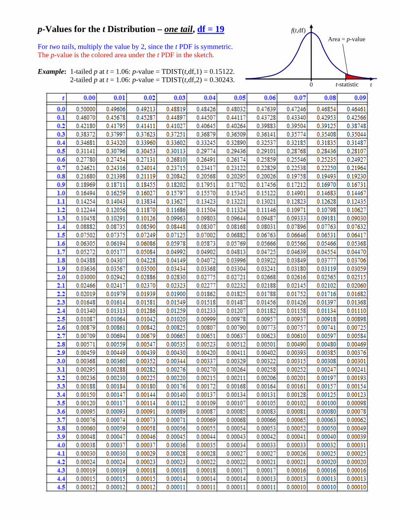
p-Values for the t Distribution – one tail, df = 19 f(t,df)

t t-statistic 0

Area = p-value For two tails, multiply the value by 2, since the t PDF is symmetric. The p-value is the colored area under the t PDF in the sketch. Example: 1-tailed p at t = 1.06: p-value = TDIST(t,df,1) = 0.15122. 2-tailed p at t = 1.06: p-value = TDIST(t,df,2) = 0.30243.

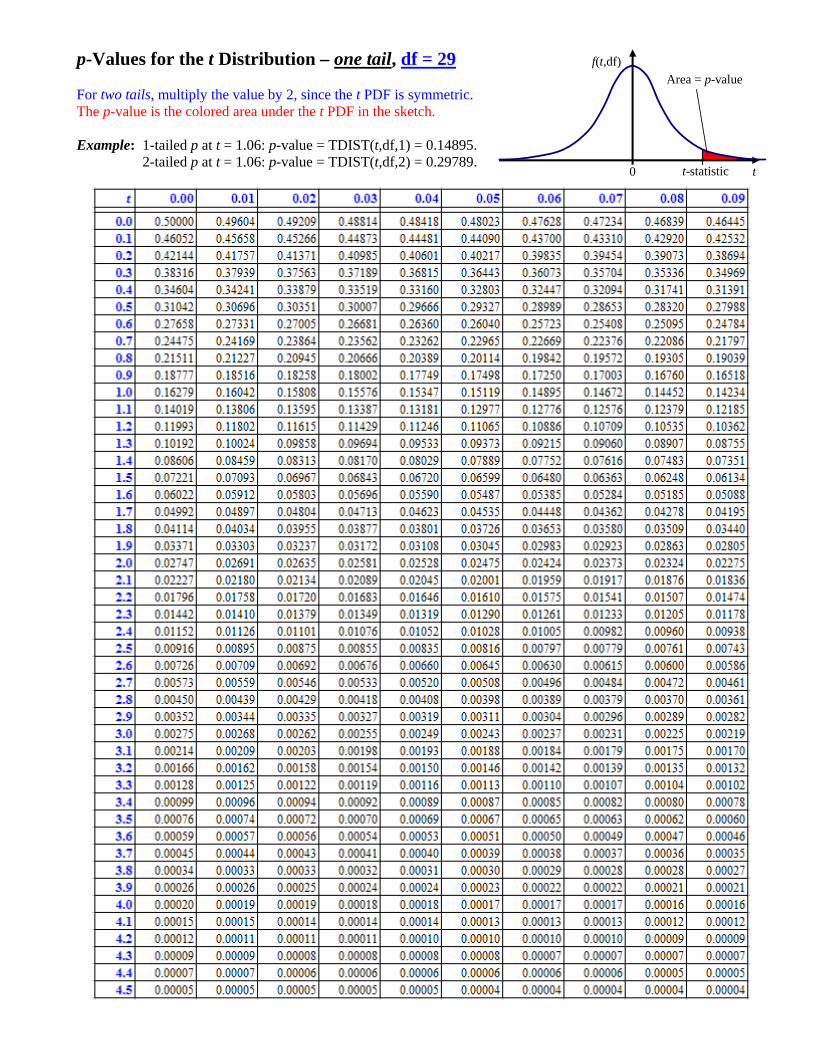
p-Values for the t Distribution – one tail, df = 29 f(t,df)

t t-statistic 0

Area = p-value For two tails, multiply the value by 2, since the t PDF is symmetric. The p-value is the colored area under the t PDF in the sketch. Example: 1-tailed p at t = 1.06: p-value = TDIST(t,df,1) = 0.14895. 2-tailed p at t = 1.06: p-value = TDIST(t,df,2) = 0.29789.

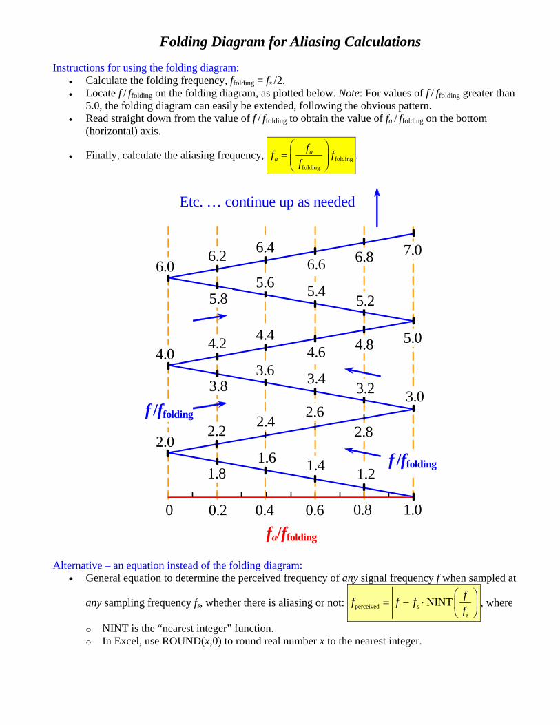
Folding Diagram for Aliasing Calculations Instructions for using the folding diagram:

• Calculate the folding frequency, ffolding = fs /2. • Locate f / ffolding on the folding diagram, as plotted below. Note: For values of f / ffolding greater than

5.0, the folding diagram can easily be extended, following the obvious pattern. • Read straight down from the value of f / ffolding to obtain the value of fa / ffolding on the bottom

(horizontal) axis.

• Finally, calculate the aliasing frequency, foldingfolding

aa

ff f

f

⎛ ⎞= ⎜ ⎟⎜ ⎟⎝ ⎠

.

0 0.2 0.4 0.6 0.8 1.0

fa/ffolding

f /ffolding

2.0 2.2

2.4 2.6

2.8

6.0

1.2 1.4 1.6

1.8

7.0 6.4 6.6 6.2 6.8

5.4 5.6

5.2 5.8

f /ffolding

3.0

4.0 5.0 4.4

4.6 4.2 4.8

3.4 3.6 3.2 3.8

Etc. … continue up as needed

Alternative – an equation instead of the folding diagram: • General equation to determine the perceived frequency of any signal frequency f when sampled at

any sampling frequency fs, whether there is aliasing or not: perceived NINTss

ff f f

f

⎛ ⎞= − ⋅ ⎜ ⎟

⎝ ⎠, where

o NINT is the “nearest integer” function. o In Excel, use ROUND(x,0) to round real number x to the nearest integer.

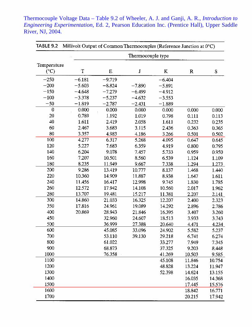
Thermocouple Voltage Data – Table 9.2 of Wheeler, A. J. and Ganji, A. R., Introduction to Engineering Experimentation, Ed. 2, Pearson Education Inc. (Prentice Hall), Upper Saddle River, NJ, 2004.

Platinum 100-Ω RTD Table

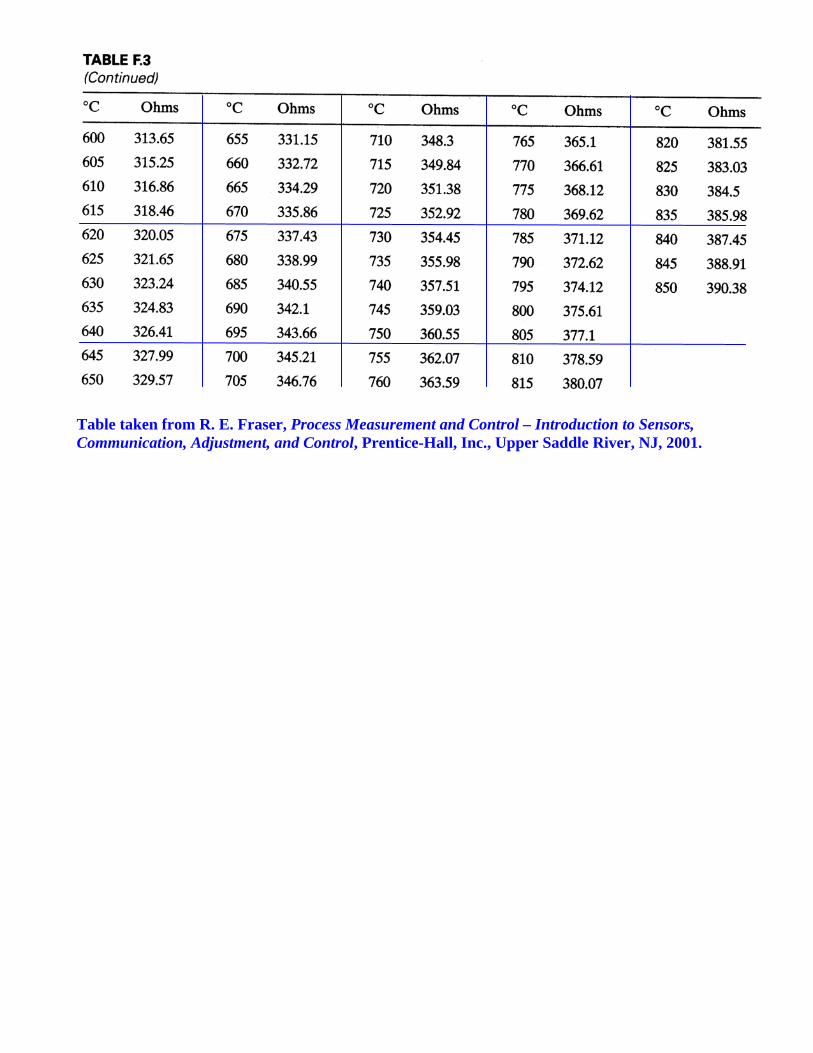
Table taken from R. E. Fraser, Process Measurement and Control – Introduction to Sensors, Communication, Adjustment, and Control, Prentice-Hall, Inc., Upper Saddle River, NJ, 2001.

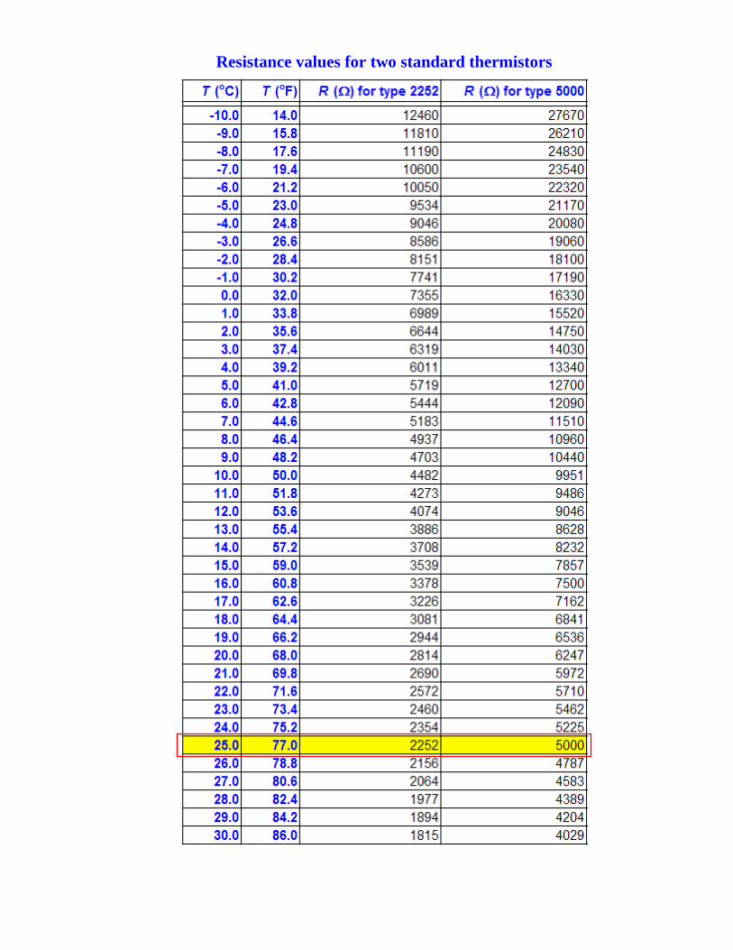
Resistance values for two standard thermistors