This is a repository copy of The thick-bedded tail of turbidite thickness distribution as a proxy for flow confinement: examples from Tertiary basins of central and northern Apennines (Italy).

White Rose Research Online URL for this paper:http://eprints.whiterose.ac.uk/99640/

Version: Accepted Version

Article:

Marini, M, Felletti, F, Milli, S et al. (1 more author) (2016) The thick-bedded tail of turbidite thickness distribution as a proxy for flow confinement: examples from Tertiary basins of central and northern Apennines (Italy). Sedimentary Geology, 341. pp. 96-118. ISSN 0037-0738

https://doi.org/10.1016/j.sedgeo.2016.05.006

© 2016 Elsevier. Licensed under the Creative Commons Attribution-NonCommercial-NoDerivatives 4.0 International http://creativecommons.org/licenses/by-nc-nd/4.0/

eprints@whiterose.ac.ukhttps://eprints.whiterose.ac.uk/

Reuse

Unless indicated otherwise, fulltext items are protected by copyright with all rights reserved. The copyright exception in section 29 of the Copyright, Designs and Patents Act 1988 allows the making of a single copy solely for the purpose of non-commercial research or private study within the limits of fair dealing. The publisher or other rights-holder may allow further reproduction and re-use of this version - refer to the White Rose Research Online record for this item. Where records identify the publisher as the copyright holder, users can verify any specific terms of use on the publisher’s website.

Takedown

If you consider content in White Rose Research Online to be in breach of UK law, please notify us by emailing eprints@whiterose.ac.uk including the URL of the record and the reason for the withdrawal request.

1

The thick-bedded tail of turbidite thickness distribution as a proxy for flow confinement: 1

examples from Tertiary basins of central and northern Apennines (Italy) 2

Mattia Marini1, Fabrizio Felletti

1, Salvatore Milli

2 and Marco Patacci

3 3

1Earth Science Department ‘Ardito Desio’, University of Milan, Italy. 4

2Earth Science Department, University of Rome ‘Sapienza’, Italy 5

3Turbidites Research Group, School of Earth and Environment, University of Leeds, Leeds, LS2 9JT, UK 6

Contact details: mattia.marini@unimi.it; ++393405865715 7

Abstract 8

The assessment and meaning of turbidite thickness statistics represent open research questions 9

for both applied and pure sedimentology. Yet thickness data collected in the field are often 10

incomplete and/or biased toward or against certain thickness classes due to bed geometry, erosion 11

and/or operational filed constraints, which largely undermine tackling such questions. However, in 12

situations where turbidity currents are ponded by basin topography so to deposit basin-wide 13

tabular beds and erosion is negligible, some of the variables of the ‘bed thickness equation’ can be 14

relaxed, making easier to investigate what the primary controls on turbidite thickness statistics are. 15

This study reviews the bed thickness statistics of the non-channelized parts of the infill of four 16

tertiary basins of Central-Northern Apennines (Italy), where bed geometry and sedimentary 17

character have been previously assessed. Though very different in terms of size and, arguably, 18

character of feeder system and source area, these basins share a common evolution to their 19

turbidite fill with upward transition from an early ponded to a late unconfined setting of deposition. 20

Based on comparison of thickness subsets from diverse locations and stratigraphic heights within 21

the basin fills of the case studies, this paper seeks to answering the following questions: i) how 22

data collection choices and field operational constraints (e.g. location, outcrop quality, use of 23

thickness from single vs. multiple correlative sections, length of the stratigraphic section from which 24

thicknesses were retrieved) can affect statistics of an empirical distribution of turbidite thicknesses? 25

ii) how depositional controls of confined vs. unconfined basins can modify the initial thicknesses 26

distribution of turbidites?; iii) is there in turbidite thickness statistics a ‘flow confinement’ signature 27

2

which can be used to distinguish between confined and unconfined depositional settings? Results 28

suggests that: i) best practices of data collection are crucial to a meaningful interpretation of 29

turbidite thickness data, especially in presence of stratigraphic and spatial trends of bed thickness; 30

ii) a systematic bias against cm-thick Tcd Bouma sequence turbidites deposited by small volume 31

low density flows exists, which can significantly modify the low-end tail of an empirical frequency 32

distribution of bed thickness; iii) thickness statistics of beds starting with a basal Ta/Tb Bouma 33

division bear a coherent relationship to the transition from ponded to unconfined depositional 34

settings, consisting in a reduction of variance and mean and, consequently, modification of the 35

initial thickness-frequency scaling relationship. This research highlights the role of flow stripping, 36

sediment by-pass and bed geometry in altering the initial thickness distribution of ponded turbidites 37

suggesting how, on the contrary, fully ponded mini-basins represents the ideal setting for further 38

research linking turbidite thickness statistics and frequency distribution of parent flow volumes. 39

Keywords: turbidites, bed thickness statistics, turbidite bed geometry, confined basin, flow 40

ponding, flow stripping 41

1. Introduction 42

Thickness variability of beds deposited by turbidity currents (turbidites hereafter) represents a 43

meaningful yet complex record of flow characteristics, flow-bathymetry interaction and bed shape. 44

Turbidite thickness data retrieved from a borehole are important in hydrocarbon system modelling 45

(Flint and Bryant, 1993) for estimation of reservoir rock volumes. Significant research efforts has 46

been dedicated to understand whether the frequency distribution of turbidite thicknesses should 47

follow a generic law, but they ended up documenting a great diversity of empirical distributions 48

(see Pickering and Hiscott, 2015 for an overview). This diversity primarily reflects a combination of 49

first order controls such as statistical distribution of inbound flow volumes, flow rheology, basin-50

floor topography, turbidite bed shape, etc. (Hiscott et al., 1992, 1993; Rothman et al., 1994; 51

Rothman and Grotzinger, 1996; Awadallah et al., 2001; Carlson and Grotzinger 2001; Talling, 52

2001; Chakraborty et al., 2002; Sinclair and Cowie, 2003; Felletti and Bersezio, 2010; Pantopoulos 53

3

et al., 2013). However, it is widely acknowledged that measured distributions might constitute 54

incomplete or biased representations of the actual thickness population owing to a number of 55

factors, (e.g. outcrop/core quality, measure/borehole location and thickness of studied/cored 56

interval; see for example Drummond and Wilkinson, 1996; Malinverno, 1997). Notwithstanding the 57

incompleteness of measured distributions, the challenge in interpreting turbidite thickness statistics 58

resides in the fact that some of the variables (e.g. bed volume and shape, including lateral extent 59

and pinch-out geometry) are unknown a priori and likely to be interdependent via complex 60

feedbacks (Janoko, 2010). In situations where erosion is negligible and turbidites are basin-wide 61

and tabular, some of the variables (e.g. bed shape, measure location, sampling biases) of the 62

turbidite thickness statistics paradigm can be fixed, making easier to study other controls (input 63

volumes, depositional controls intrinsic to confinement etc). This condition is commonly met in 64

small turbidite basins enclosed by a confining topography (i.e., confined basins; see Lomas and 65

Joseph, 2004), where flows large enough can spread over the entire depocentre and become 66

ponded, therefore depositing basin-wide sheet-like turbidites (see paragraph 2.1). 67

This study investigates the stratigraphic variability of bed thickness statistics of the distal non-68

channelized parts of four confined to unconfined turbidite units of northern and central Italy, the 69

‘Cengio, Bric la Croce – Castelnuovo’ turbidite systems and Castagnola Formation of the Tertiary 70

Piedmont Basin and the Laga and Cellino formations of the Apennines foreland basin system. 71

The primary focus of this paper is nor finding a general statistical model for turbidite thickness 72

distribution, neither methods for best-fitting empirical data, on which the literature is vast (Goldstein 73

et al., 2004; Clauset et al. 2009; Sylvester, 2007; Cirillo, 2013). Instead, this paper aims at 74

answering the following questions: i) how do data collection choices and/or field operational 75

constraints (e.g. use of thickness from single vs. multiple correlative sections, length of the 76

stratigraphic section, location with respect to basin topography, outcrop quality etc.) affect the 77

statistical appraisal of frequency distribution of turbidite thicknesses? ii) Is there a turbidite 78

thickness statistics signature of flow confinement that can be used to distinguish between confined 79

4

and unconfined depositional settings? iii) How do depositional controls of confined vs. unconfined 80

basins modify the initial thicknesses distribution of turbidites? 81

2. Overview of turbidite thickness statistics 82

Early research on frequency distribution of turbidite thickness mostly focused on finding which 83

model better described empirical datasets, and if such a law was somehow generic to turbidite 84

deposition (e.g. truncated Gaussian, lognormal, exponential and power-law; see Sylvester, 2007 85

for an overview). In most of these studies, distribution models better describing empirical thickness 86

populations were chosen through visual inspection of a number of graphical tools, such as 87

histograms and log-log plots of exceedance probability (i.e. plots with logarithmic scale on both 88

horizontal and vertical axes relating the number of beds thicker than a given thickness h, to h; Fig. 89

1). However, as case studies grew in number, it became obvious that, other than sharing an 90

inverse relationship of thickness against number of beds (i.e. thinner beds are more numerous that 91

thicker beds), empirical distributions departed significantly from simple statistical models and 92

differed greatly from each other, especially in their thin-bedded tails (see Pickering and Hiscott, 93

2015 for an overview). Based on the assumption that a generic law describing turbidite thickness 94

existed, a number of factors (e.g., sampling bias against thin beds, non-deposition by small volume 95

flows not reaching the sampling site, erosion; Drummond and Wilkinson, 1996) were used to 96

explain scarcity of very thin beds in log-normal distributions (McBride, 1962; Ricci Lucchi, 1969; 97

Ricci Lucchi and Valmori, 1980; Murray et al., 1996) and in truncated Gaussian distributions 98

(Kolmogorov, 1951; McBride, 1962; Mizutani and Hattori, 1972) when compared to exponential 99

distributions (Muto, 1995; Drummond, 1999; see also Chakraborty et al., 2002). For analogy with 100

some of the most common triggers of turbidity currents (e.g., submarine sand avalanche and 101

earthquakes) and other geological quantities (e.g., fault lengths, volcanic eruptions and drainage 102

networks; Turcotte, 1997), another line of thought (Hiscott et al., 1992, 1993; Beattie and Dade, 103

1996; Rothman et al., 1994; Rothman and Grotzinger, 1996) proposed that the frequency 104

distribution of turbidite thickness should follow a power-law exceedance probability equation: 105

5

N(H>h) = Ntotalh-く (1) 106

where N is the number of beds of thickness H greater than h, Ntotal is the total number of beds and 107

く is the scaling exponent of the power-law relationship. Equation (1) plots as a straight line on a bi-108

logarithmic (log-log) graph (Fig. 1) and is typically valid above a threshold value or lower bound 109

denoted as xmin. An implication of such power-law relationship is that the bed thickness distribution 110

is scale invariant and completely described by the scaling exponent く, which would therefore 111

represent a fractal dimension (Turcotte, 1997). Due to the great popularity of fractality in nature, 112

from the 1990s onwards most of the empirical distributions showing convex-upward shapes on a 113

log-log exceedance probability plot were interpreted as ‘segmented’ distributions resulting from 114

modification of a power-law input signal (i.e. the distribution of volumes of flows entering the basin). 115

The sharp cross-over in the scaling exponent く of ‘segmented’ distributions was variously 116

interpreted as resulting from sampling biases, erosion and/or undetected amalgamation, flow 117

rheology transitions and flow-basin topography interactions (Rothman and Grotzinger, 1995; 118

Malinverno, 1997; Chen and Hiscott, 1999; Carlson and Grotzinger, 2001; Awadallah et al., 2002; 119

Sinclair and Cowie, 2003; Felletti and Bersezio, 2010). The power-law paradigm was later 120

challenged on the ground that ‘segmented’ distributions can result from mixing of two or more sub-121

populations of beds each characterized by a log-normal distribution (Talling, 2001; Sylvester, 2007; 122

Pantopoulos et al., 2013). In this ‘log-normal mixture’ model, the sub-populations are characterised 123

by different basal grain size or sedimentary structures and the sharp gradient cross-over of many 124

thickness probability plots is interpreted as associated to differences in the parent flow (e.g. low 125

density vs. high density turbidity currents). 126

2.1. Controls on deposition of ponded turbidites and on resulting bed thickness statistics 127

In turbidity currents’ mechanics, confinement is the ability of the seafloor topography to obstruct or 128

redirect the flow thereby inducing perturbation of its velocity field and physical structure (Joseph 129

and Lomas, 2004). Interaction with obstacles of size comparable to or larger than the height of 130

incoming flows, such as bounding slopes of enclosed mini-basins, can result in a range of 131

6

modifications within the flow (e.g. reflection/deflection, constriction, ponding and flow stripping; see 132

Patacci et al., 2015), producing unusual vertical sequences of sedimentary structures (Kneller et 133

al., 1991; Haughton, 1994; Kneller and McCaffrey, 1999; Bersezio et al., 2005, 2009; Tinterri 134

2011). Upon impact onto bounding slopes, the density stratification of turbidity currents typically 135

results in trapping of the lower, higher-density and sandier part of the flow in the deeper part of the 136

basin and stripping (sensu Sinclair and Tomasso, 2002) of the more dilute and muddier upper part 137

of the flow, which can partially escape the basin by surmounting the topography or overflowing a 138

local sill. Ponding represents a case of confinement, whereby the entire flow is trapped by the 139

topography (Van Andel and Komar, 1969). When sustained large flows are discharged into a 140

receiving basin, flow ponding can result in the development of a flat-topped sediment cloud (i.e. the 141

ponded suspension cloud; Toniolo et al., 2006; Patacci et al., 2015). Ponding and flow stripping 142

processes are intimately related in that if the total volume discharged by a turbidity current is larger 143

than the volume of the receiving basin, the ponded suspension cloud can thicken up to partially 144

overflow the confining topography (Patacci et al., 2015; Marini et al., 2016), with establishment of 145

partially ponded conditions. The most striking sedimentary signature of ponding are basin-wide 146

couplets of sands with multiple repetitions of sedimentary structures and relatively thick co-genetic 147

mud caps (Ricci Lucchi and Valmori, 1980; Pickering and Hiscott, 1985; Haughton, 1994; Kneller 148

and McCaffrey, 1999). Conversely, similarly to by-pass in unconfined systems, in partially ponded 149

conditions, flow stripping can deplete turbidites of their finer-grained fraction resulting in 150

sandstones with unusually thin fine-grained laminated tops and mud caps (Sinclair and Tomasso, 151

2002; Marini et al., 2016). Common examples of confined-ponded turbidite systems are found in 152

structurally-controlled elongated basins, such as wedge-top basins of foreland basin systems 153

(Remacha et al. 2005; Milli et al., 2007, 2009; Tinterri and Tagliaferri, 2015), rift basins (Ravnås 154

and Steel, 1997; Ravnås et al, 2000) and intraslope salt-withdrawal mini-basins (Prather et al. 155

2012). The initial topography of these basins is generally able to fully pond incoming flows (i.e. all 156

the sediment is trapped within the basin) leading to development of a sheet-like architecture. 157

However, when sedimentation rate outpaces tectonic deformation, sediment infilling can result in 158

7

enlargement of the local depocentre and decrease of the height of the enclosing slopes. 159

Consequently, the degree of flow confinement decreases and the proportion of sediments 160

escaping the basin increases (Remacha et al. 2005; Felletti and Bersezio, 2010; Marini et al. 2015, 161

2016), in a manner similar to that described by the classical ‘fill to spill’ model of Sinclair and 162

Tomasso (2002). 163

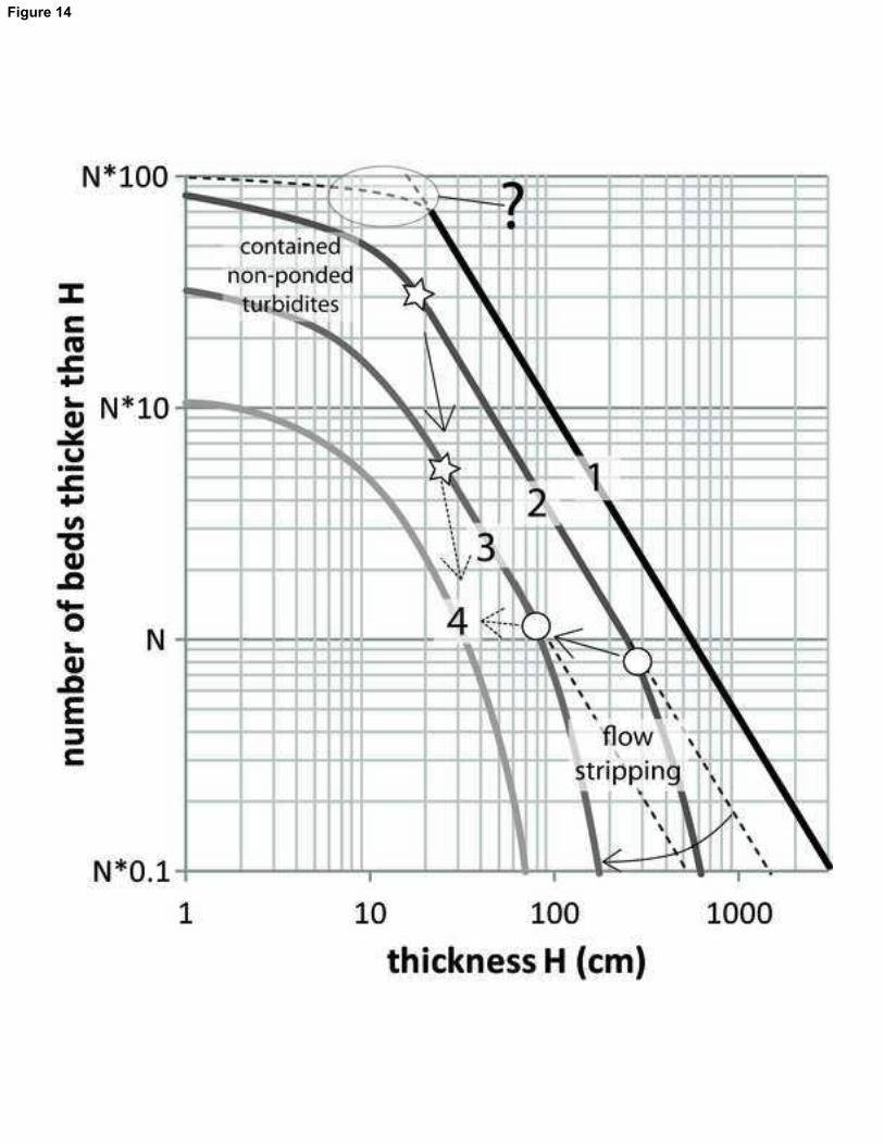
The effect of confinement on turbidite thickness distribution is amenable to numerical experiments 164

(Malinverno, 1997; Sylvester, 2007), simulating measurement of bed thickness along a vertical 165

sampling line located at the centre of a circular enclosed mini-basin. These experiments used a 166

large number of model beds turbidites with cylindrical shape, power-law volume frequency 167

distribution and fixed scaling of bed length to thickness to demonstrate that if beds are placed at 168

random within the basin then the log-log plot of exceedance probability of thicknesses measured 169

along a sampling line at the basin centre will break into three linear segments (Fig. 2a). These 170

segments correspond to subpopulations of: i) relatively thin turbidites with diameter smaller than 171

the radius of the receiving basin, which form a first segment with slope くsmall as a result of being 172

undersampled (not all of them are encountered by the sampling line; ii) turbidites of intermediate 173

thickness and diameter equal to or greater than the basin diameter, which are always intersected 174

by the sampling line and form a segment of the distribution with slope くlarge and iii) basin-wide 175

turbidites (i.e. turbidites with diameter greater than the basin diameter), namely mega-beds that are 176

ponded by the receiving topography, which form a linear segment of the distribution with slope 177

くlarge>くmega≥くsmall (Fig. 2a). As claimed by Sylvester (2007), though very simplistic with regard to 178

geometry of model beds, the model of Malinverno (1997) might be able to produce ‘segmented’ 179

power-law distributions with the provisos that volumes of incoming turbidity currents must show a 180

power-law frequency distribution and bed thickness is measured at or very close to basin centre. 181

Other numerical experiments (Sinclair and Cowie, 2003) showed that if all the turbidity currents 182

entering a mini-basin are ponded (i.e. all the sediment is trapped in the basin) and volumes of 183

incoming flows follow a power-law distribution, then the resulting bed thicknesses will scale to 184

8

volumes as a function of bed length and size of the mini-basin (Fig. 2b). Modifications of a power-185

law input signal have been also linked to flow stripping and erosional bed amalgamation (Sinclair 186

and Cowie, 2003). Specifically, in partially ponded basins flow stripping of the upper and finer-187

grained part of large volume (and thicker) currents acts by limiting the total amount of sediment 188

trapped in the basin so that the bed thickness population is depleted in its thick-bedded tail (Fig. 189

2b). 190

3. Methodology 191

The thickness data considered in this study were taken and revised from earlier works by the 192

authors (Felletti et al., 2009; Felletti and Bersezio, 2010; Marini et al. 2015, 2016), to which the 193

reader is referred for details of the locations and sedimentological descriptions. The compound 194

database therefore comprises as many datasets as the studied turbidite units (Table 1), each 195

consisting of a number of stratigraphic and location subsets, i.e. sets of thickness measures 196

collected from specific stratigraphic intervals of the case study on a single section within the basin. 197

As discrimination of hemipelagic from turbiditic mudstone was not always practical due to outcrop 198

quality, thereby preventing in some instances to correctly place the upper boundary of turbidite 199

event beds and measure their thickness, the choice was made to work with sandstones only. 200

Therefore, if not specified otherwise, ‘bed thickness’ is used here to refer to the sandstone part of 201

turbidites. Bed thickness was measured from the base of the sandstone to the boundary between 202

very fine silty sandstone and mudstone, using a tape meter for thinner beds (thickness range 1-50 203

cm) and a Jacob’s staff for beds thicker than c. 50 cm (see Patacci, 2016 for a review on error 204

sources when measuring bed thicknesses). The thickness of the mudstone above was recorded 205

separately, noting whether the quality of the outcrop allowed it to be interpreted as a mud cap 206

genetically related to the underlying turbidite sandstone. The basal grain size of the sandstone was 207

measured using a magnifying lens and a grain size comparator, thereby allowing for detection of 208

subtle grading breaks and correct placing of boundaries of single event beds within amalgamated 209

bedsets. As it was believed that hybrid beds (sensu Haughton et al. 2009), namely beds deposited 210

9

by flows including a frontal turbidity current and a lagging co-genetic debris flow, may have a 211

significantly different depositional mechanism, after calculating their relative frequency (generally 212

below 6%) they were excluded from the analysis. To facilitate comparisons across case studies, 213

turbidites were classified according to the same bed type scheme, based on sedimentological 214

character and grain size of their basal division. Two main bed type classes were distinguished: a) 215

beds consisting of Tc and/or Td Bouma (1962) divisions with typical basal grain size finer than 250 216

たm and thickness generally less than 30-50 cm, and b) beds starting either with a basal Ta or Tb 217

Bouma divisions coarser than 250 たm which may grade upward into finer sands with variously 218

developed Tc-d divisions (thickness generally greater than 10-30 cm). Although there is much more 219

complexity in the turbidites of the studied examples (for which the reader is referred to relevant 220

literature given in Table 1), this simple bed type scheme has the advantage of objectively 221

discriminating between two classes, namely the deposits of low and high density flows (see Lowe, 222

1982 and discussion in Talling, 2001). Prior to undertaking data analysis, an assessment of the 223

effects of sampling procedures on thickness statistics was carried out by comparing subsets from 224

different stratigraphic intervals and locations (see paragraph 5.1). Following such an assessment, 225

further statistical analysis was focused only on thickness subsets from single sections either 226

located as close as possible to the basin centre or, when basin shape was uncertain, the farthest 227

possible from basinal slopes. Best fitting with three model distributions (i.e. exponential, log-normal 228

and power-law) commonly used in turbidite thickness statistics was performed using the Easyfit 229

software package. Easyfit uses the maximum likelihood estimation method (MLE) to assess 230

parameters of log-normal and power-law fits whereas fitting with the exponential model is based on 231

the method of moments. In both fitting methods, the number of iterations and the accuracy of MLE 232

was set to 100 and 10-5, respectively. Goodness-of-fit testing was accomplished with the same 233

software using the Kolmogorov-Smirnov (K-S), the Chi-Squared (激2) and the Anderson-Darling (A-234

D) tests. All of these tests assess the compatibility of a random sample (i.e. the empirical 235

distribution of turbidite thickness measured in the field) with a theoretical probability distribution 236

function (i.e. the model distribution), that is how well the model distribution fits empirical data. This 237

10

is accomplished computing test statistics (see for example Table 2) that quantify how much the 238

cumulative distribution function of an empirical dataset departs from that of the model distribution 239

and comparing the obtained values to standard tables of critical values compiled in the Easyfit for 240

different significance levels (0.01, 0.05 etc.). In this study a significance level of 0.1 was applied, 241

that is, there is 10% probability that the model distribution passing the tests is not an adequate fit. 242

For 激2 a equal probability binning was adopted which follows the law: 243

k = 1+log2(N) (2) 244

where k is the number of bins and N the number of beds in the sample data. In addition to test 245

statistics p-values are also computed in K-S and 激2 which may be considered as a measure of 246

plausibility of the model distribution being a good fit for the empirical distribution being tested. 247

Specifically, while small values of p shed doubt on the goodness of the fit, large values of p do 248

neither prove it nor demonstrate evidence against it. The most likely parent distribution reported in 249

Table 2 were chosen taking into account goodness of fit results of the three tests and p-values 250

jointly, with the provisos that since standard table for critical values were used, though equally with 251

respect to whichever model, results of the tests are conservative.As the bed types subset for which 252

a power-law model cannot be excluded based on the adopted goodness-of-fit tests comprised less 253

then ≈50 beds, in agreement with the assessment of Clauset et al. (2009) on the minimum sample 254

size (≈100) required for successfully distinguishing between a power-law and a log-normal as the 255

best fit option, the decision was made to not implement the procedure for using of K-S proposed by 256

these Authors. Yet, not using boothstrapping (see Clauset et al., 2009) for estimating the lower 257

bound xmin of the power-law fit of bed types subsets, might not represent a limitation to the purpose 258

of this study, as best fitting was intended for being tied to facies and parent flow characteristics 259

rather than bed thickness alone. 260

As an independent mean to characterize the thick-bedded tails of our empirical frequency 261

distributions and quantify their location and spread (i.e. statistical dispersion of a dataset), 262

summary statistics including mean, quantiles, interquartile ranges (i.e. the difference between the 263

11

75% and the 25% quantiles) and coefficient of variation (i.e. the ratio of standard deviation to 264

mean) were also calculated (Isaaks and Srivastava, 1989). 265

4. Case studies 266

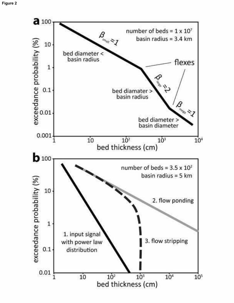
The turbidite units considered in this study represent parts of the infill of the Tertiary Piedmont 267

Basin of NW Italy and of the latest Miocene – early Pliocene Apennine foreland basin system of 268

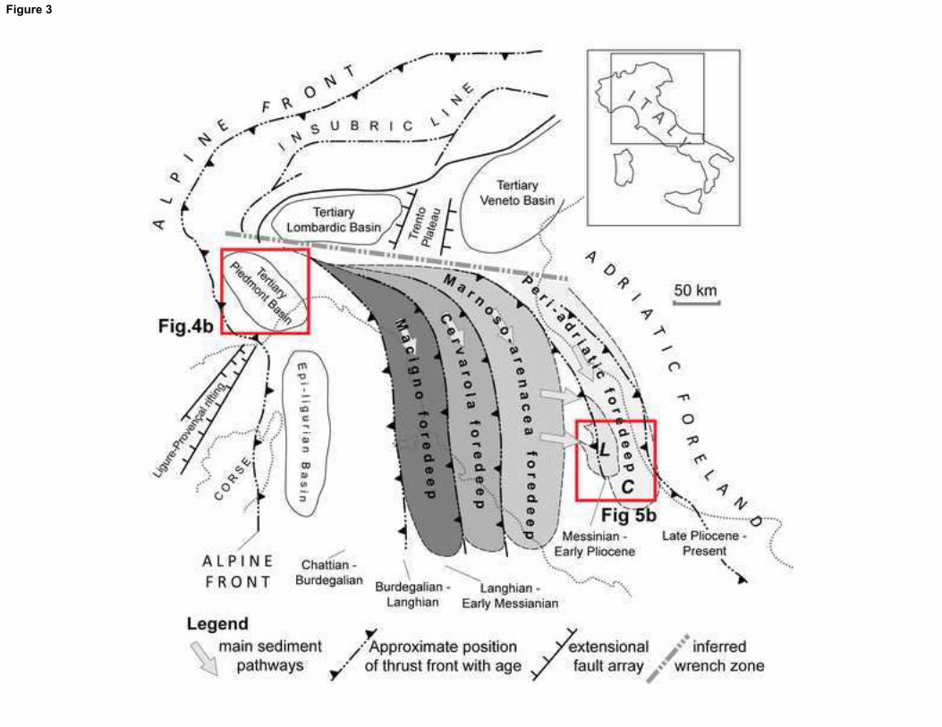
central Italy (Fig. 3 and Table 1). The Tertiary Piedmont Basin (TPB hereafter) is a relatively small 269

yet complex wedge-top basin (Figs 3 and 4) located at the junction between the westward-verging 270

stack of tectonic nappes of Western Alps and the north-eastward verging Northern Apennines 271

(Mosca et al. 2010; Carminati and Doglioni, 2012; Maino et al. 2013; Ghibaudo et al., 2014a, b). It 272

consists of two main sub-basins, namely the Langhe Basin to the west and the Borbera-Curone 273

Basin to the east (Gelati and Gnaccolini, 1998; Mosca et al., 2010), which side the Alto Monferrato 274

structural high (Fig. 4) and host up to 4000 m of continental to deep marine clastic sediments. The 275

clastic infill of these sub-basin records Early Oligocene – Burdigalian extensional tectonics related 276

to the opening of the Ligure-Provençal Basin (Gelati and Gnaccolini, 2003). 277

The foreland basin system of the Central Apennines is a large palaeogeographic domain 278

developing from the Oligocene onwards in response to the westward subduction of a promontory 279

of the African Plate (i.e. the Adria microplate) underneath the European plate (Malinverno and 280

Ryan, 1986; Vai, 2001; Boccaletti et al., 1990; Carminati and Doglioni, 2012). Roll back of the 281

subducting plate led to eastward migration of both the accrectionary wedge and the adjacent 282

foredeep which was filled by diachronous turbidite units (Fig. 3) younging from west to east (Ricci 283

Lucchi, 1986). These include four main foredeep turbidite infills, namely the Macingo Formation 284

(Chattian-Burdigalian), the Cervarola-Falterona Formation (Burdigalian-Langhian), the Marnoso 285

Arenacea Formation (Langhian-Lower Messinian) and the Cellino Formation (Lower Pliocene; see 286

paragraph 4.4) supplied axially with sediments from Alpine sources. A number of smaller turbidite 287

bodies of Messinian age (including the Laga Formation, see paragraph 4.3) were also deposited 288

within scattered structurally-confined wedge-top basins (‘bacini minori’ of Centamore et al, 1978) 289

12

with mostly transverse feed (Fig. 3). Establishment and infilling of these basins records the 290

accretion of the Marnoso Arenacea into the orogenic wedge (Ricci Lucchi, 1986; Manzi et al., 291

2005) and pre-dates the onset of the late Messinian – Pliocene periadriatic foredeep, respectively. 292

The Castagnola Formation (CS). It represents the infill of one of the sub-basins of the Borbera-293

Curone sector (Castagnola Basin; Fig. 4) and consists of a >950 m-thick turbidite succession of 294

Late Chattian-Early Burdigalian age. It was deposited in a slightly elongated structural depression 295

forming southward of the ENE–WSW striking Villalvernia-Varzi Line (V-V in Fig. 4; Cavanna et al., 296

1989; Mutti, 1992; Stocchi et al., 1992, Di Giulio and Galbiati, 1998) and running parallel to it. CS 297

has been subdivided into three members (Baruffini et al., 1994), namely, from older to younger, the 298

Costa Grande, Arenaceo and the Brugi Marls members. While the older two members are 299

represented almost exclusively by turbidites, the younger Mt. Brugi Marls Member consists of 300

mostly silicified marly hemipelagites with intercalations of thin bedded turbidites. Well exposed 301

onlaps onto basinal slopes (Felletti, 2002; Southern et al., 2015) indicate an initial depocentre with 302

size of c. 4x2 km (length x width) which might have increased up to a minimum of c. 6x4 km (length 303

x width) as a result of infilling by turbidites of the Costa Grande Member. Early research (Cavanna 304

et al., 1989; Stocchi et al., 1992) documented a change in architectural style from the sheet-like 305

and relatively mud-rich Costa Grande Member, consisting of basin-wide sandstone-mudstone 306

couplets, to the sand-rich Arenaceo Member. typified by lenticular and locally amalgamated 307

turbidite sandstones. More recently, stratigraphic trends in sand-to-mud ratio and facies have been 308

interpreted to reflect the transition from a dominantly ponded sheet-like system (Costa Grande 309

Member) to a non-ponded system (Arenaceo Memmber) (Marini et al., 2016). 310

The stratigraphy and process sedimentology of the CS has been recently addressed (Marini et al., 311

2016) by means of a highly detailed sedimentological section logged at the basin centre. The most 312

significant stratigraphic trend in this turbidite unit is the steady increase in sand-to-mud ratio from 313

base to top. In the uppermost c. 200 m of the studied section this is accompanied with replacement 314

of basin-wide sandstone-mudstone cap couplets with a ponded character (bed types A and B of 315

13

Southern et al., 2015 cf. ‘contained beds’ of Pickering and Hiscott, 1985; see also Haughton, 1994; 316

Sinclair, 1994), by locally amalgamated turbidites with thin fine-grained tops (bed type B’ of Marini 317

et al., 2016) suggestive of by-pass. In addition, whilst Bouma-like Tcd turbidites (bed types D of 318

Southern et al., 2015; typically thinner than c. 30 cm) are ubiquitous in the studied section forming 319

a background to clusters of thicker beds, their relative frequency appear to decrease upward in the 320

stratigraphy. These trends culminate in the transition from a lower, relatively shale-prone sections 321

(unit 1 and unit 2 of Marini et al. 2016; CS-1 and CS-2 hereafter) punctuated by thick beds with a 322

ponded character, including thick mud caps, by a upper sand-rich section where by-pass of fines 323

and event bed amalgamation dominate (unit 3; CS-3 hereafter). If thicknesses of mud caps of 324

turbidites from CS-1 and CS-2 are looked at into greater detail, a weak but negative correlation of 325

their thickness proportion and total thickness of event beds to which they belong can be seen, 326

hinting at some dependency of the amount of mud the basin topography was able to trap on total 327

volume of incoming turbidity currents. The stratigraphy of CS was interpreted as embodying a 328

threefold ‘fill to spill’ evolution of the host basin (Marini et al., 2016), including: i) an early ponded 329

stage (CS-1) in which only part of the mud of exceptionally large flows could escape the basin, ii) 330

an intermediate stage (CS-2) when levelling of the initial topography by turbidite infilling resulted in 331

enhanced flow spilling, possibly affecting also a fraction of the sand of exceptionally large flows 332

and iii) a late by-pass stage (CS-3) where turbidite systems were virtually unconfined and could 333

expand over an healed topography. 334

Cengio (CTS) and Bric la Croce - Castelnuovo (BCTS) turbidite systems. These are two 335

superimposed turbidite systems of Late Oligocene age infilling a structurally-confined depocentre 336

set along the western slope of the Langhe Basin of TPB (Fig. 4) (Gelati and Gnaccolini, 1980; 337

Cazzola et al., 1981, 1985; Mutti, 1992; Gelati and Gnaccolini, 1998, 2003; Felletti and Bresezio, 338

2010; Felletti, 2016). Deposition of CTS and BCTS took place in a period of quiescent tectonics 339

(sequences B2-3 of Gelati and Gnaccolini, 1998) within a SW-NE-trending structural trough 340

supplied with turbidity flows from the southwest. While the southern, western and northern 341

bounding slope of the CTS - BCTS depocentre are well exposed, uncertainty exists about the 342

14

eastern margin of the basin, which might have been located a few km away from the studied 343

outcrop, i.e. at the structural culmination of basement rocks (Gelati and Gnaccolini, 1980; Cazzola 344

et al., 1981). The transition from ponded sheet-like turbidites of the lower CTS (sandbodies I and II; 345

Bersezio et al. 2005, 2009) to unconfined lobes of the BCTS via non-ponded, but laterally confined 346

lobes of the upper CTS (sandbodies III-VIII; Bersezio et al., 2009) is interpreted to reflect a 347

significant enlargement of the local depocentre due to sediment infill (Felletti and Bersezio, 2010; 348

Felletti, 2016). 349

Based on numerous stratigraphic sections from different locations with respect to basinal slopes, 350

previous workers (Bersezio et al., 2005, 2009; Felletti and Bersezio, 2010) documented an 351

increased degree of bed amalgamation and sand-to-mud ratio toward onlap terminations and 352

greater proportions of massive sands at the base of confining slopes. Coupled with palaeoflow 353

indicators, these trends suggest redirection and blocking of the lower, denser part of flow. 354

Conversely, from proximal to distal (i.e. from SW to NE), Bersezio et al. (2005) reported a 355

decrease in sand-to-mud and laminated-to-massive sandstone ratios and average thickness of the 356

sandstone beds. 357

Away from basinal slopes, the most common bed type in both CTS and BCTS is represented by 358

massive to laminated, graded sandstones with very thin or missing rippled tops (top-missing 359

Bouma sequences; cf bed types D, E and DB of Bersezio et al. 2005). These beds occur in both 360

thin bedded, well stratified mud-prone intervals and sand-rich packages. In the latter, they can lack 361

any mud cap and be welded to form amalgamated bedsets, but only rarely show basal scours (up 362

to a few cm’s deep), suggesting little erosion from subsequent flows. Other bed types include 363

variously developed Bouma-like sequences, which can be either complete or miss Ta/Tb divisions. 364

In CTS these beds can internally show repeated sequences of sedimentary structures (‘complex’ 365

beds sensu Bersezio et al. 2005, 2009), interpreted as the product of instabilities induced in the 366

flow by interaction with basinal slopes (see Kneller and McCaffrey 1999; Tinterri, 2011). Whichever 367

the bed type, it is noteworthy that the thickness of the sandstone and the mud cap of event beds 368

15

have only very limited negative correlation, with thicker beds showing thinner mud caps with 369

respect to thinner beds. The widespread by-pass indicators (e.g. reduced thickness of fine-grained 370

rippled tops and mud caps, hints of anticorrelation of mud cap and sandstone thickness within 371

event beds) in both CTS and BCTS, coupled with proximal to distal variability in bed thickness and 372

mud content (Bersezio et al., 2005) indicates that, while incoming turbidity currents unquestionably 373

interacted with the north and north-western basinal slopes, neither their sandy nor muddy part 374

were ponded by the receiving topography over most of the studied section. 375

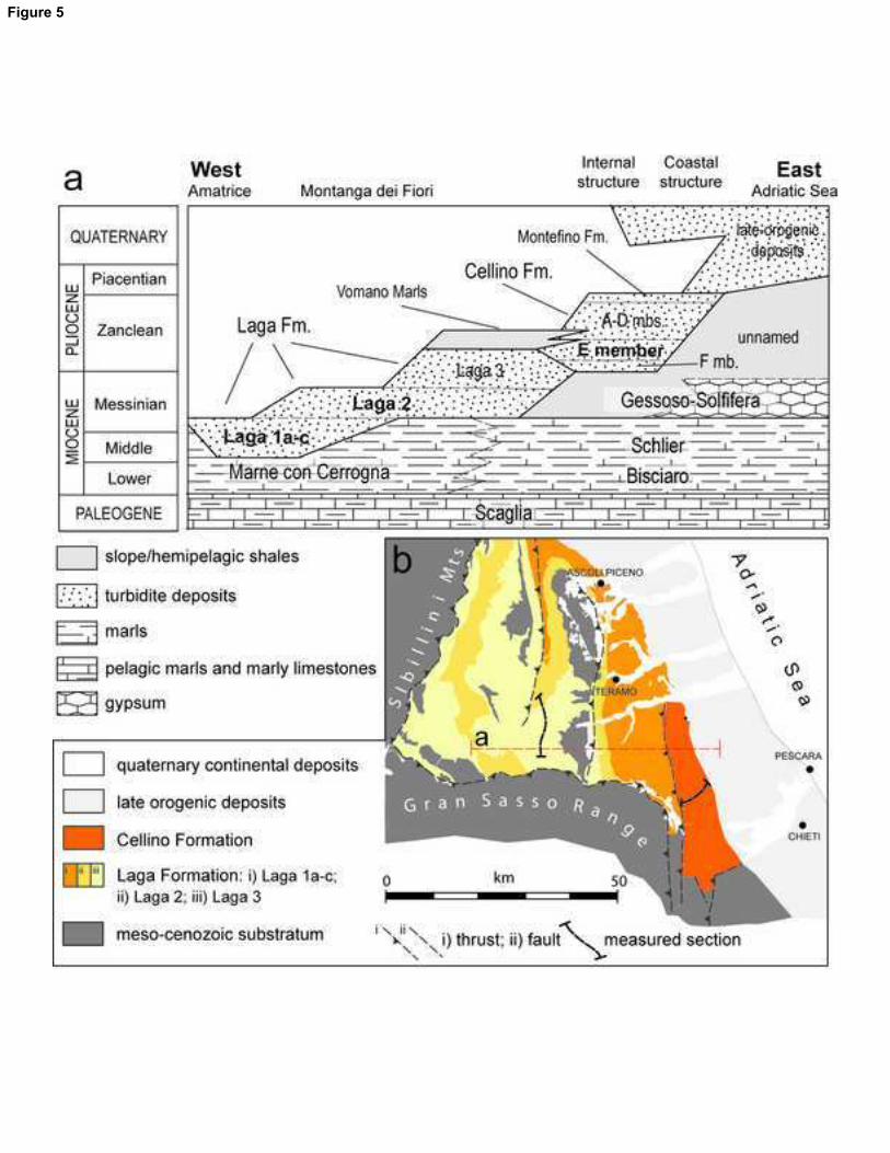
The Laga Formation lobes (LG). The Laga Formation constitutes the c. 3000-thick turbidite infill 376

of a relatively large wedge-top basin (i.e. the Laga Basin; Figs 3 and 5b) developed since the late 377

Tortonian in response to tectonic fragmentation of the Marnoso Arenacea foredeep (Manzi et al., 378

2005; Milli et al., 2007). LG is composed of five unconformity-bounded units (Laga 1a, 1b, 1c, 2 379

and 3), correlatable to main tectonic-stratigraphic events of the Messinian (Milli et al., 2007, 2009, 380

2013). They can be grouped into two high rank depositional sequences, namely the Laga 381

Depositional Sequence (Laga 1a-c and Laga 2, upper Tortonian-lower Upper Messinian) and the 382

Cellino Depositional Sequence (Laga 3 and younger deposits of the Vomano and Cellino Fms.; 383

Upper Messinian – Lower Pliocene). These sequences display a eastward stacking and are 384

separated by a main erosional unconformity (the intra-Messinian unconformity) recording an acme 385

of tectonic shortening and uplift along the thrust front of Central Apennine (Ricci Lucchi, 1986; 386

Manzi et al., 2005; Milli et al., 2007). The deposition of the Laga 1a-c and Laga 2 took place in a 387

confined ‘piggy-back’ basin swallowing and enlarging as a result of turbidite infill (Fig. 5a), whereas 388

the Laga 3 unit records the onset of the Pliocene to present-day foreland basin systems (Milli et al., 389

2007, 2009; Bigi et al. 2009). From north to south, physical stratigraphy and facies analysis of the 390

Laga 1-2 turbidite systems document along-stream transition from proximal distributive networks of 391

low-sinuosity channels to distal lobes (i.e., LG) and an overall stratigraphic evolution from a more 392

confined to less confined setting of deposition (Milli et al., 2007, 2009, 2013; Marini et al., 2015). 393

16

The thickness data used in this study come from three superimposed lobe units, namely, from 394

older to younger, the Poggio Umbricchio (LG-1), the Crognaleto (LG-2) and the Mt. Bilanciere (LG-395

3) lobe complexes, deposited in a depocentre enlarging considerably (by a factor in excess of 3.5, 396

see Table 1) as a result of infilling from turbidites. LG-1 has the highest sand-to-mud ratio 397

compared to the two younger lobe complexes and it is characterized by higher proportion of 398

massive-looking dewatered sandstones, coarser and less sorted grain size and thinner mud caps. 399

It has been suggested that while the structureless character of the sandstones of LG-1 might 400

reflect rapid sediment dumping resulting from blocking of the flows by the confining topography, the 401

low mud content in the same unit would indicate either spilling of finer grained sediments or an 402

initial coarser-grained sediment input (Marini et al. 2015). Two contrasting styles of depositional 403

architecture have been recently documented in these units, specifically a sheet-like architecture 404

composed of mostly basin-wide event beds, such as that of the two older complexes (LG-1 and 405

LG-2), and a ‘jig-saw-like’ architecture typified by the laterally shifting lobes of the younger complex 406

(LG-3) (Marini et al. 2015). Lateral facies changes in beds of LG-1 and LG-2 are limited to the 407

vicinity of bounding slopes thus reflecting a primary control from flow-topography interactions. On 408

the contrary, beds of LG-3 show a higher but regular lateral variability in bed character (thickness, 409

grain size and proportion of massive vs. laminated sands decrease from proximal to distal and 410

across palaeoflow) suggestive of deposition from unconfined turbidity currents losing competence 411

and capacity away from the centre of mass of lobes. In all the units, thin bedded Bouma-like Tcd 412

turbidites cluster into metre to decametre-scale packages correlatable over most of the depocentre 413

without significant changes in facies, grain size and sand content, suggesting they are unlikely to 414

represent turbidite lobe fringes. 415

As suggested by the increase in size of the local depocentre, the change of architectural style was 416

interpreted as a shift from partially ponded (LG-1) and confined (LG-2) conditions, to unconfined 417

conditions (LG-3) favouring deposition of lobate sandbodies with compensational stacking (Marini 418

et al. 2015; see also Mutti and Sonnino, 1981). 419

17

Cellino Formation (CL). This turbidite unit of Early Pliocene age represents the over 2500m-thick 420

infill of the inner sector (namely, the Cellino Basin) of the Pliocene to present-day foreland basin 421

system of the Apennines. Due to limited outcrop, most of the knowledge about the size and 422

geometry of the Cellino Basin is owed to a wealth of seismic and well data made available by the 423

intense hydrocarbon exploration undertaken from the 50’s to the 70’s of the last century (Casnedi 424

et al., 1976 Casnedi, 1983; Vezzani et al. 1993) (Figs. 3 and 5). Correlation between outcrops and 425

geophysical well logs allowed tracking CL in the subsurface for over c. 40 km and up to 150 km in 426

a E-W and N-S directions, respectively (Carruba et al. 2004, 2006), and detailing the architecture 427

of its six members (A to F from top to bottom; Casnedi, 1983). 428

This study focuses on the c. 750 m-thick sand-rich section of the E member only, which represents 429

the early confined infill of a N-S trending foredeep supplied with flows from the north (Felletti et al. 430

2009). The thickness data presented in this paper are located in the southernmost part of the basin 431

(Barricello section; see Felletti et al. 2009 for details). Lateral thickness changes in the older F 432

member reveal some initial unevenness of the seafloor at the onset of turbidite deposition. 433

However, the correlation framework of the E member indicates the early establishment of a 434

relatively large (Table 1) yet confined depocentre, filled in with a sheet-like succession composed 435

of sand-rich clusters of thick-bedded turbidites intercalated with few m to few tens of m-thick 436

packages of thin bedded turbidites (Carruba et al. 2004; Felletti et al. 2009). Isopach maps and 437

basin-scale correlations of the E member hint at a gradual decrease in the gradient of the basinal 438

slopes, suggesting that the degree of confinement of its turbidite systems might have reduced 439

swiftly because of infilling from turbidites. The sand-rich thick-bedded component of the E member 440

includes two main turbidite types: i) Ta-missing or complete Bouma sequence turbidites (few tens 441

of cm to less than c. 190 cm), interpreted as the product of waning surge-like flows, and ii) very 442

thick beds and megabeds (thickness in range of c. 270-1200 cm) with massive bases which grade 443

upward into thick laminated intervals with repeated sequences of sedimentary structures. Typically, 444

the latter bed type is capped by thick mud caps which, together with the well structured character 445

of the sandstone below suggest deposition from long-lived turbidity currents ponded by the basin 446

18

topography (Felletti et al. 2009, cf. with ‘contained beds’ of Pickering and Hiscott, 1985). These two 447

types of thick-bedded turbidite show contrasting bed planforms as well, with Bouma-like turbidites 448

tapering distally and being generally smaller than the receiving depocentre as opposed to beds 449

with a ponded character being tabular and basin-wide (Felletti et al. 2009). The thin-bedded 450

component of the E member constitutes a significant fraction of the stratigraphy (c. 25 % of the 451

total thickness) and includes both Tcd Bouma sequence turbidites starting with a basal sand and 452

way more numerous cm-thick silty turbidites (Td Bouma divisions) locally intercalated with 453

hemipelagites. Although all of the bed types are ubiquitous in the studied section, there is a 454

stratigraphic trend toward reduction of both the thickness of ‘ponded’ megabeds and typical ratio of 455

mud cap to sandstone thickness of event beds from the lower to the upper half of the E member 456

(CL-1 and CL-2, respectively). Keeping with the geometry of the southern basinal slope (Carruba 457

et al. 2004), this trend hints at a swift increase of the depocentre size as a result of sediment 458

infilling and, possibly, onset of a late ‘spill’ phase in which a fraction of the finer grained part of 459

larger incoming flows could escape the basin. 460

5. Results 461

5.1. Assessment of sampling biases affecting turbidite thickness statistics 462

In statistical analysis, a sample is a set of observations drawn from a population through a 463

procedure devised to minimize sampling biases (Stuart, 1962). However, especially if the variable 464

of interest is non-stationary in a xyz space and its population structure (including spatial trends) is 465

unknown a priori, a random (or probability-based) sampling procedure cannot be trusted even 466

when the number of samples is very large. In turbidite sedimentology spatial trends appear to be 467

the rule rather than the exception, therefore a sound analysis of thickness statistics requires careful 468

assessment of the following sources of sampling bias: i) a bed thickness dataset retrieved from a 469

continuous section measured in a wellbore or in the field is representative of an interval of 470

stratigraphic thickness z, which may contain turbidite systems with different sets of external 471

controls; ii) in presence of spatial trends of turbidite thickness (e.g. laterally tapering beds related to 472

19

stratigraphic pinch-outs, lobe shapes, channel fills), i.e. when thickness is non-stationary in xy, 473

thickness data retrieved from a sampling location of given x, y coordinates can be biased toward or 474

against certain thickness classes; iii) the number of thinner beds might be underestimated (see 475

Drummond and Wilkinson, 1996) because thin bedded turbidites have a lower preservation 476

potential of thicker beds due to erosion by subsequent flows or biogenic mottling (Weathercroft, 477

1990), they generally form shaly sections prone to cover from scree and vegetation and are 478

impractical to detect even on good outcrops when they are finer-grained than coarse silt. 479

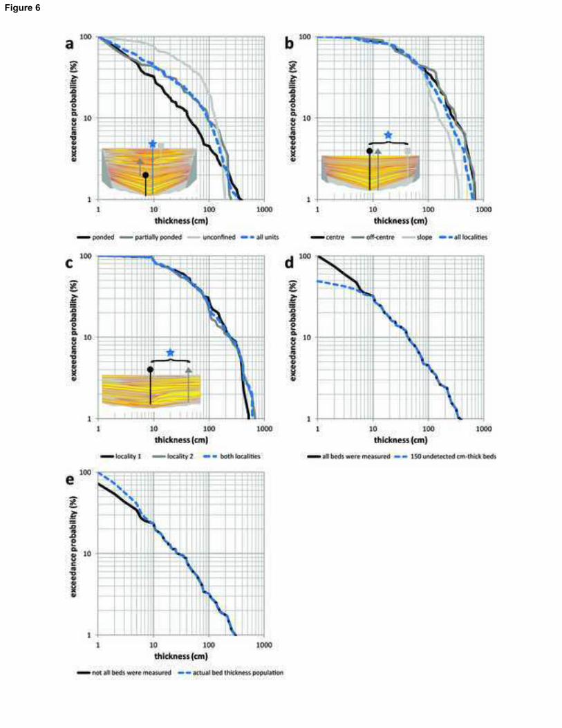
To get insights into the first sampling issue, turbidite thicknesses from the each of the three 480

stratigraphic subsets of the Castagnola Fm, (CS, hereafter; see paragraphs 4.1 and 5.2.1) are 481

plotted together with the full dataset of the same case study. The stratigraphic subsets of CS (CS-482

1, CS-2, and CS-3 in Fig 6a) were defined by Marini et al. (2016) based on stratigraphic trends (i.e. 483

changes in facies types, sand-to-mud ratio) which, with the support of independent observations on 484

basin size, suggest different depositional processes and controls. It is therefore no surprise that the 485

thickness statistics for these subsets and for the whole CS dataset are very different from each 486

other (Figs 6a) and so do best-fitting results (Table 2). 487

The bias inherent to sampling location when a systematic spatial trend of thickness is present is 488

illustrated in Fig 6b which compares data from two different correlative sections from the confined 489

sheet-like Crognaleto lobe complex of the Laga Formation (LF hereafter; see paragraphs 4.3 and 490

5.2.3) at the basin centre and above the onlap onto the bounding slope. It can be noted that the 491

thick-bedded tail of the subset from the onlap is shifted to the left compared to that of the basin 492

centre, because the turbidites progressively thin approaching the slope (Fig 6b). In agreement with 493

the overall sheet-like nature of the Crognaleto lobe complex, such bias toward thinner beds 494

disappears when the sampling location moves away from the slope (cf. ‘off-centre’ with ‘centre’ in 495

Fig 6b). Surprisingly enough, if two subsets c. 1 km apart from the laterally shifting lobes of the 496

semi-confined Mt. Bilanciere lobe complex of LF (see paragraphs 4.3 and 5.2.3) are compared (Fig 497

6c), it is apparent that sampling location does not influence the shape of the curve. This can be 498

20

explained by the memoryless and randomness nature of the compensational stacking of 499

component beds of turbidite lobes (Mutti and Sonnino, 1981; Prelat and Hodgson, 2013), which 500

makes two outcropping sections or boreholes not very far apart to intercept lobate geometries 501

randomly, thereby resulting in similar empirical thickness distributions at the two locations if section 502

thickness is at least several times larger than the average lobe thickness. 503

The modification of the ‘true’ frequency distribution of turbidite thicknesses arising from not 504

detecting in the field the deposit of all of the flows entering a confined mini-basin is illustrated in Fig 505

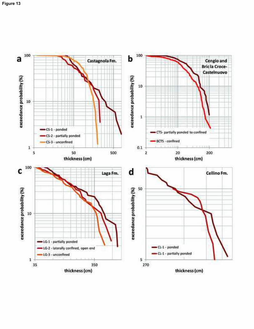
6d-e using two simple yet meaningful experiments. Such experiments are grounded on the 506

observation that, while bed correlatability between the two sections measured by Marini et al. 507

(2016) c. 2.5 km apart is 100% for turbidites thicker than c. 10 cm, below this thickness threshold 508

nearly 50% of the beds measured at one location cannot be identified at the other location. The 509

reason for this correlation mismatching could be that because cm-thick turbidite sandstones 510

typically have a basal grain size close to the limit between very fine sand and coarse silt, lateral 511

fining of the deposit can make these beds difficult to identify across the whole basinal area. 512

Alternatively, another possible explanation is that not all the very thin beds in the field could be 513

identified because of usually poorer exposure of shale-prone thin bedded intervals. We anticipate 514

here that best fitting of the CS-1 subset suggests a log-normal model and an exponential model as 515

plausible parent distributions for the full range of measured thickness (‘all beds’) and for the 516

subpopulation of beds starting with a basal Tc or Td Bouma division, respectively (Table 2). In Fig 517

6d the subset of CS-1 (378 beds) is plotted besides a synthetic dataset decimated of an arbitrary 518

number of 150 very thin beds in order to simulate an enhanced effect of underdetection. The 519

decimated dataset (228 beds) was generated by removing a percentage of the beds thinner than 520

10 cm from the full subset. The percentage of beds removed was higher for very thin beds (45% of 521

beds <1 cm were removed), and diminished linearly up to a minimum of 5% for beds of 8-9 cm of 522

thickness. Fig 6d illustrates that the underdetection of thin beds results in the down bending of the 523

low-end tail and an increased upward convexity of the exceedance probability plot of CS-1 and, 524

presumably, in a modification of the parameters of the empirical distribution. 525

21

The experiment of Fig 6d assumes that the correlation mismatch documented in the nearby 526

sections of the Castagnola Basin is due to lateral fining of the deposit and that in the field it was 527

possible to measure the thickness of any deposit coarser than fine silts and therefore that CS-1 528

represents the actual turbidite thickness population. However, if less than good exposition of shale-529

prone intervals were the reason for undersampling of thin beds, what we should have done in Fig 530

6d was adding, rather than subtracting such a fraction of beds as for Fig. 6e. Including a 531

‘conservative’ number of 150 undetected beds thinner than 10 cm results in the thin-bedded tail of 532

the exceedance probability plot of CS-1 to be visibly modified which, again, might be accompanied 533

by a severe modification of the parameters of the empirical distribution(Fig. 6e). 534

Observations from the reported case studies show that in certain stratigraphic intervals thin beds 535

are densely packed and form metre- to 10s metre-thick shale-prone packages (typical thin bed 536

frequency is in order of 5 to 15 per metre). In these cases, an effect similar to that shown in Fig 6e 537

can result from a short (less than 10 m) shaly interval of a stratigraphic section impossible to 538

measure bed by bed for being intensely mottled due to bioturbation or covered. 539

5.2. Bed thickness statistics of the case studies 540

5.2.1. The Castagnola Formation (CS) 541

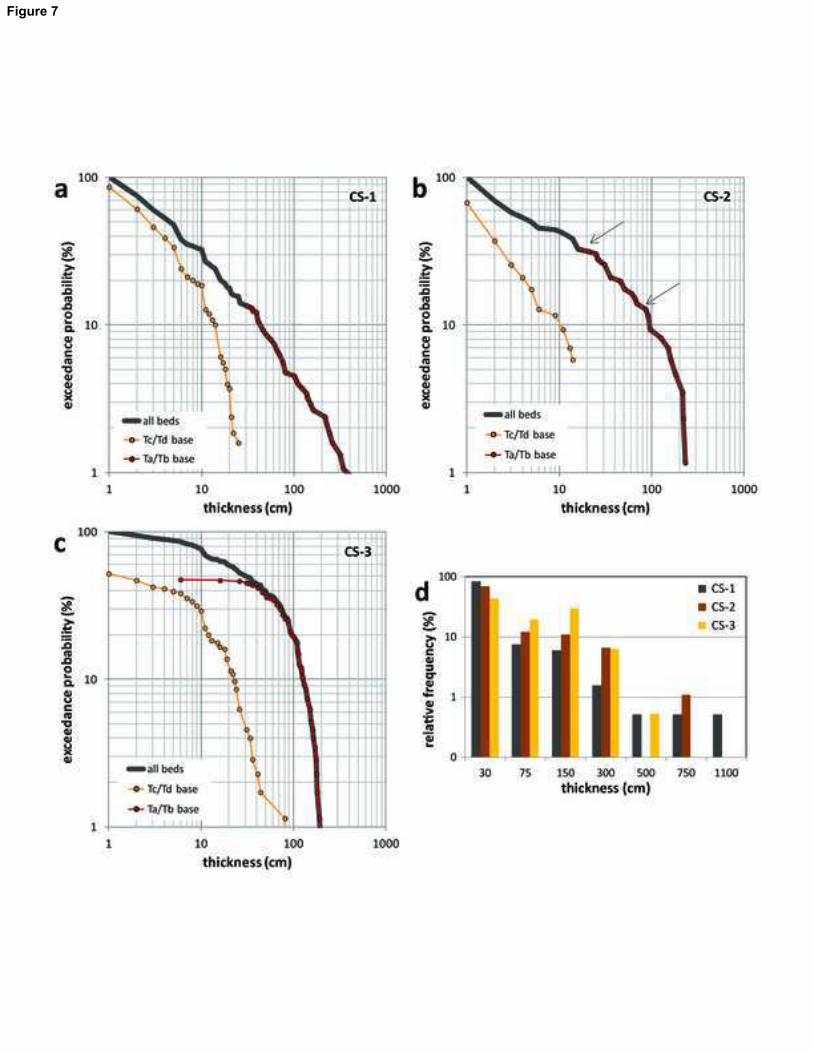
Exceedance probability plots suggest different statistical distributions for the three stratigraphic 542

subsets (‘all beds’, black lines in Fig. 7a-c), with CS-1 showing a very gentle upward convexity by 543

way of a subtle gradient change across a thickness threshold of c. 30 cm, as opposed to the 544

markedly convex upward shapes of CS-2 and CS-3 plots. Albeit any of these subsets fails to pass 545

goodness-of-fit tests (Table 2), test statistics suggest a log-normal model as the best fitting choice. 546

If thicknesses of CS-1 turbidites are plotted as separate bed type subsets, we can note how the 547

aforesaid gradient change corresponds to the breakpoint between the thin and thick bed 548

subpopulations, which show no or negligible overlap. While best fitting results (Table 2) suggests 549

that the first subset has been likely drawn from a population with an exponential distribution (cf. 550

with Fig. 1), a power-law model turns out to be the best fit for the second subset, holding for more 551

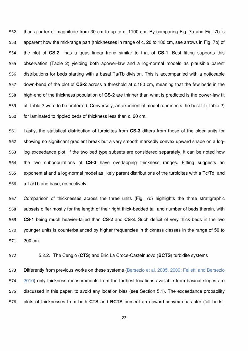
22

than a order of magnitude from 30 cm to up to c. 1100 cm. By comparing Fig. 7a and Fig. 7b is 552

apparent how the mid-range part (thicknesses in range of c. 20 to 180 cm, see arrows in Fig. 7b) of 553

the plot of CS-2 has a quasi-linear trend similar to that of CS-1. Best fitting supports this 554

observation (Table 2) yielding both apower-law and a log-normal models as plausible parent 555

distributions for beds starting with a basal Ta/Tb division. This is accompanied with a noticeable 556

down-bend of the plot of CS-2 across a threshold at c.180 cm, meaning that the few beds in the 557

high-end of the thickness population of CS-2 are thinner than what is predicted is the power-law fit 558

of Table 2 were to be preferred. Conversely, an exponential model represents the best fit (Table 2) 559

for laminated to rippled beds of thickness less than c. 20 cm. 560

Lastly, the statistical distribution of turbidites from CS-3 differs from those of the older units for 561

showing no significant gradient break but a very smooth markedly convex upward shape on a log-562

log exceedance plot. If the two bed type subsets are considered separately, it can be noted how 563

the two subpopulations of CS-3 have overlapping thickness ranges. Fitting suggests an 564

exponential and a log-normal model as likely parent distributions of the turbidites with a Tc/Td and 565

a Ta/Tb and base, respectively. 566

Comparison of thicknesses across the three units (Fig. 7d) highlights the three stratigraphic 567

subsets differ mostly for the length of their right thick-bedded tail and number of beds therein, with 568

CS-1 being much heavier-tailed than CS-2 and CS-3. Such deficit of very thick beds in the two 569

younger units is counterbalanced by higher frequencies in thickness classes in the range of 50 to 570

200 cm. 571

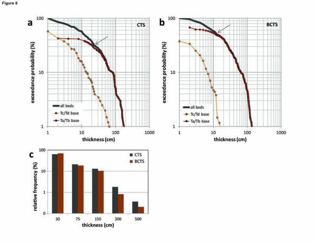
5.2.2. The Cengio (CTS) and Bric La Croce-Castelnuovo (BCTS) turbidite systems 572

Differently from previous works on these systems (Bersezio et al. 2005, 2009; Felletti and Bersezio 573

2010) only thickness measurements from the farthest locations available from basinal slopes are 574

discussed in this paper, to avoid any location bias (see Section 5.1). The exceedance probability 575

plots of thicknesses from both CTS and BCTS present an upward-convex character (‘all beds’, 576

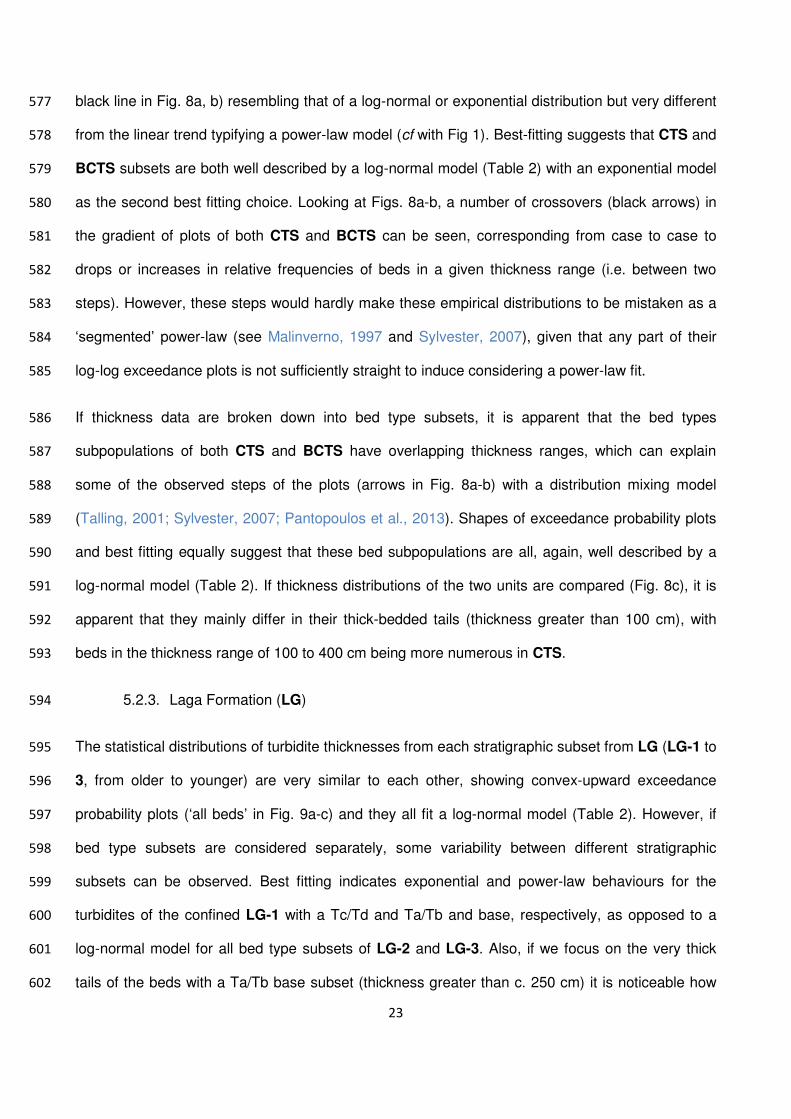
23

black line in Fig. 8a, b) resembling that of a log-normal or exponential distribution but very different 577

from the linear trend typifying a power-law model (cf with Fig 1). Best-fitting suggests that CTS and 578

BCTS subsets are both well described by a log-normal model (Table 2) with an exponential model 579

as the second best fitting choice. Looking at Figs. 8a-b, a number of crossovers (black arrows) in 580

the gradient of plots of both CTS and BCTS can be seen, corresponding from case to case to 581

drops or increases in relative frequencies of beds in a given thickness range (i.e. between two 582

steps). However, these steps would hardly make these empirical distributions to be mistaken as a 583

‘segmented’ power-law (see Malinverno, 1997 and Sylvester, 2007), given that any part of their 584

log-log exceedance plots is not sufficiently straight to induce considering a power-law fit. 585

If thickness data are broken down into bed type subsets, it is apparent that the bed types 586

subpopulations of both CTS and BCTS have overlapping thickness ranges, which can explain 587

some of the observed steps of the plots (arrows in Fig. 8a-b) with a distribution mixing model 588

(Talling, 2001; Sylvester, 2007; Pantopoulos et al., 2013). Shapes of exceedance probability plots 589

and best fitting equally suggest that these bed subpopulations are all, again, well described by a 590

log-normal model (Table 2). If thickness distributions of the two units are compared (Fig. 8c), it is 591

apparent that they mainly differ in their thick-bedded tails (thickness greater than 100 cm), with 592

beds in the thickness range of 100 to 400 cm being more numerous in CTS. 593

5.2.3. Laga Formation (LG) 594

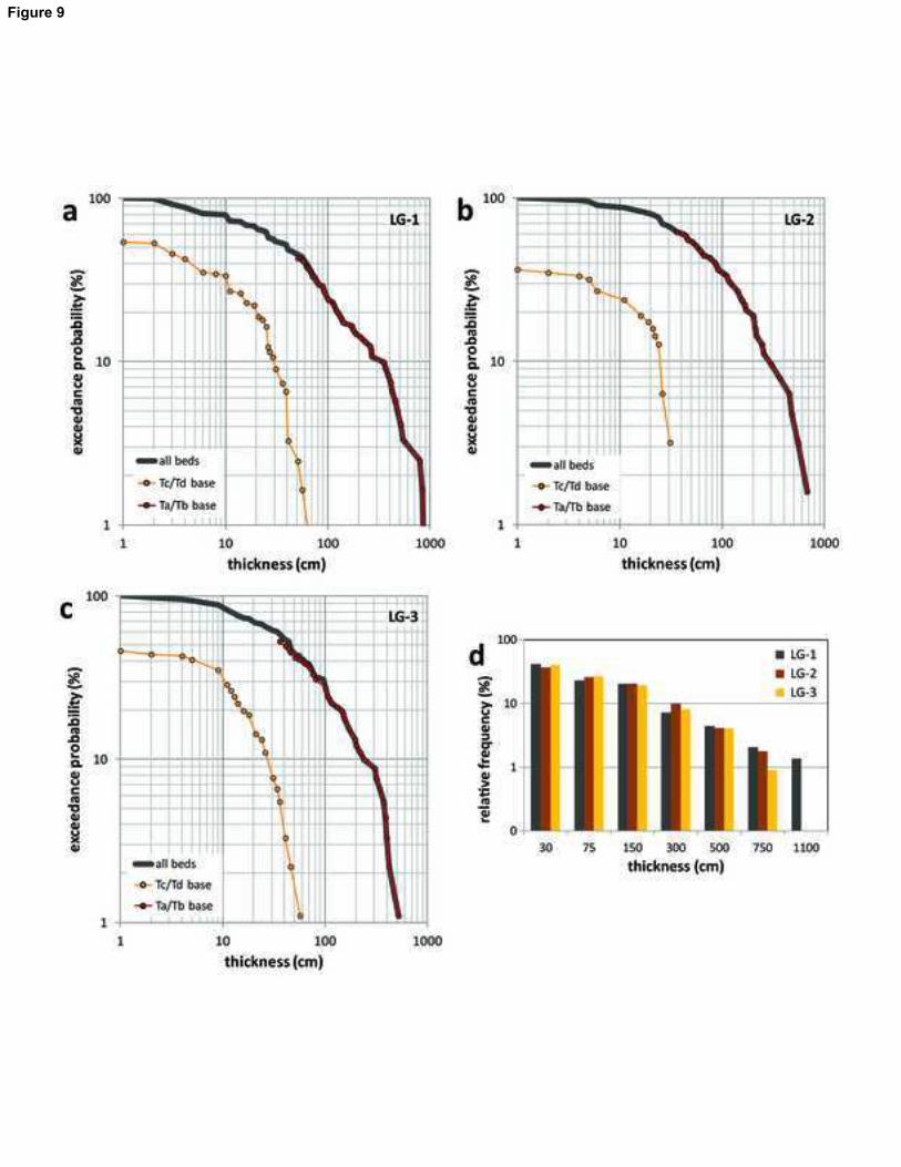
The statistical distributions of turbidite thicknesses from each stratigraphic subset from LG (LG-1 to 595

3, from older to younger) are very similar to each other, showing convex-upward exceedance 596

probability plots (‘all beds’ in Fig. 9a-c) and they all fit a log-normal model (Table 2). However, if 597

bed type subsets are considered separately, some variability between different stratigraphic 598

subsets can be observed. Best fitting indicates exponential and power-law behaviours for the 599

turbidites of the confined LG-1 with a Tc/Td and Ta/Tb and base, respectively, as opposed to a 600

log-normal model for all bed type subsets of LG-2 and LG-3. Also, if we focus on the very thick 601

tails of the beds with a Ta/Tb base subset (thickness greater than c. 250 cm) it is noticeable how 602

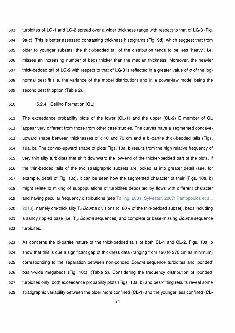
24

turbidites of LG-1 and LG-2 spread over a wider thickness range with respect to that of LG-3 (Fig. 603

9a-c). This is better assessed contrasting thickness histograms (Fig. 9d), which suggest that from 604

older to younger subsets, the thick-bedded tail of the distribution tends to be less ‘heavy’, i.e. 605

misses an increasing number of beds thicker than the median thickness. Moreover, the heavier 606

thick-bedded tail of LG-2 with respect to that of LG-3 is reflected in a greater value of j of the log-607

normal best fit (i.e. the variance of the model distribution) and in a power-law model being the 608

second best fit option (Table 2). 609

5.2.4. Cellino Formation (CL) 610

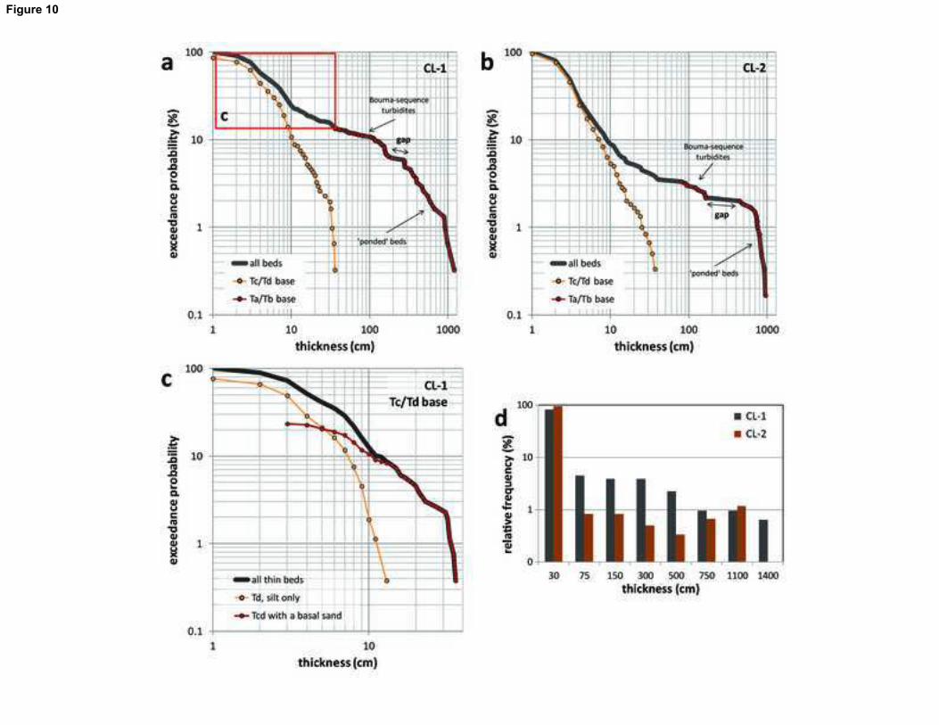
The exceedance probability plots of the lower (CL-1) and the upper (CL-2) E member of CL 611

appear very different from those from other case studies. The curves have a segmented concave-612

upward shape between thicknesses of c.10 and 70 cm and a bi-partite thick-bedded tails (Figs. 613

10a, b). The convex-upward shape of plots Figs. 10a, b results from the high relative frequency of 614

very thin silty turbidites that shift downward the low-end of the thicker-bedded part of the plots. If 615

the thin-bedded tails of the two stratigraphic subsets are looked at into greater detail (see, for 616

example, detail of Fig. 10c), it can be seen how the segmented character of their (Figs. 10a, b) 617

might relate to mixing of subpopulations of turbidites deposited by flows with different character 618

and having peculiar frequency distributions (see Talling, 2001; Sylvester, 2007; Pantopoulos et al., 619

2013), namely cm-thick silty Td Bouma divisions (c. 80% of the thin-bedded subset), beds including 620

a sandy rippled base (i.e. Tcd Bouma sequences) and complete or base-missing Bouma sequence 621

turbidites. 622

As concerns the bi-partite nature of the thick-bedded tails of both CL-1 and CL-2, Figs. 10a, b 623

show that this is due a significant gap of thickness data (ranging from 190 to 270 cm as minimum) 624

corresponding to the separation between non-ponded Bouma sequence turbidites and ‘ponded’ 625

basin-wide megabeds (Fig. 10c). (Table 2). Considering the frequency distribution of ‘ponded’ 626

turbidites only, both exceedance probability plots (Figs. 10a, b) and best-fitting results reveal some 627

stratigraphic variability between the older more confined (CL-1) and the younger less confined (CL-628

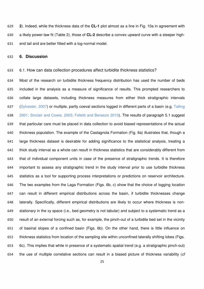
25

2). Indeed, while the thickness data of the CL-1 plot almost as a line in Fig. 10a in agreement with 629

a likely power-law fit (Table 2), those of CL-2 describe a convex upward curve with a steeper high-630

end tail and are better fitted with a log-normal model. 631

6. Discussion 632

6.1. How can data collection procedures affect turbidite thickness statistics? 633

Most of the research on turbidite thickness frequency distribution has used the number of beds 634

included in the analysis as a measure of significance of results. This prompted researchers to 635

collate large datasets, including thickness measures from either thick stratigraphic intervals 636

(Sylvester, 2007) or multiple, partly coeval sections logged in different parts of a basin (e.g. Talling 637

2001; Sinclair and Cowie, 2003; Felletti and Bersezio 2010). The results of paragraph 5.1 suggest 638

that particular care must be placed in data collection to avoid biased representations of the actual 639

thickness population. The example of the Castagnola Formation (Fig. 6a) illustrates that, though a 640

large thickness dataset is desirable for adding significance to the statistical analysis, treating a 641

thick study interval as a whole can result in thickness statistics that are considerably different from 642

that of individual component units in case of the presence of stratigraphic trends. It is therefore 643

important to assess any stratigraphic trend in the study interval prior to use turbidite thickness 644

statistics as a tool for supporting process interpretations or predictions on reservoir architecture. 645

The two examples from the Laga Formation (Figs. 6b, c) show that the choice of logging location 646

can result in different empirical distributions across the basin, if turbidite thicknesses change 647

laterally. Specifically, different empirical distributions are likely to occur where thickness is non-648

stationary in the xy space (i.e., bed geometry is not tabular) and subject to a systematic trend as a 649

result of an external forcing such as, for example, the pinch-out of a turbidite bed set in the vicinity 650

of basinal slopes of a confined basin (Figs. 6b). On the other hand, there is little influence on 651

thickness statistics from location of the sampling site within unconfined laterally shifting lobes (Figs. 652

6c). This implies that while in presence of a systematic spatial trend (e.g. a stratigraphic pinch-out) 653

the use of multiple correlative sections can result in a biased picture of thickness variability (cf 654

26

‘centre+slope’ with ‘centre’ and ‘off-centre’ plots in Fig 6b) and should therefore be avoided, in the 655

case of turbidite beds with spatially random thickness variations it can provide a larger dataset with 656

virtually no bias if the study section is sufficiently thick (cf ‘all’ plot with those of each of the different 657

locations in Fig 6c). Finally, the experiments of Figs. 6d-e simulate the effect of undersampling of 658

cm-thick turbidites with similar results to that of Malinverno (1997), and illustrates how even in an 659

enclosed ponded mini-basin a considerable number of very thin depositional events are likely to be 660

not detected also on fairly good outcrops. Further and even more severe sources of bias against 661

thin beds include local erosion by subsequent flows (Drummond and Wilkinson, 1996; Sinclair and 662

Cowie, 2003) and bioturbation (Weathercroft, 1990). 663

6.2. What are the implications of the bias against thin beds? 664

The under detection of the number of thin turbidite beds discussed in the previous section is 665

particularly relevant when attempting to fit an empirical frequency distribution of turbidite thickness 666

with existing model distributions. This is because, since turbidites typically show an inverse 667

relationship between number of beds and thickness, the thin-bedded part of any empirical 668

distribution is statistically so ‘weighty’ (e.g., in the studied datasets turbidites with thickness less 669

than c. 30 cm typically represent more than 60% of the total number of beds) that it literally acts as 670

a ‘watershed’ between alternative model distributions (e.g. log-normal vs. exponential and power-671

laws; see Fig. 1). The results of the experiments of Figs. 6d-e show how under detection of very 672

thin beds can impact the low-end of empirical distributions, making for some ambiguity of fitting 673

results not accompanied with an assessment of such type of bias. A quantification of the bias 674

against thin beds resulting because or erosion by subsequent flows or, alternatively, biogenic 675

mottling is provided by works by Kolmogorov (1951) and Muto (1995) which demonstrate that a 676

significant part of the low-end tail of the actual bed thickness distribution may be not preserved in 677

certain turbidite successions. 678

27

6.3. Stratigraphic variability of the thick-bedded tails of the case studies 679

After appraising likely biases related to data collection, we are now left with finding a way to 680

compare the bed thickness statistics of different stratigraphic subsets and case studies. The 681

sensitivity of the thin-bedded part of any turbidite thickness population to undersampling (see 682

paragraphs 6.1 and 6.2), suggests that for an unbiased evaluation the focus should be on the 683

reminder part of the thickness population. This could be done by either choosing a thickness cut-684

off, e.g. 10 cm, above which in good outcrop conditions it is reasonable to assume that all 685

sandstone beds were detected or working with the thick-bedded subpopulation of the empirical 686

datasets, namely that including only turbidites starting with a basal Ta/Tb Bouma division. 687

Here, the second approach is preferred because it restricts the treatment to the deposits of large 688

volume turbidity currents that reached the measure location with similar initial rheology and were 689

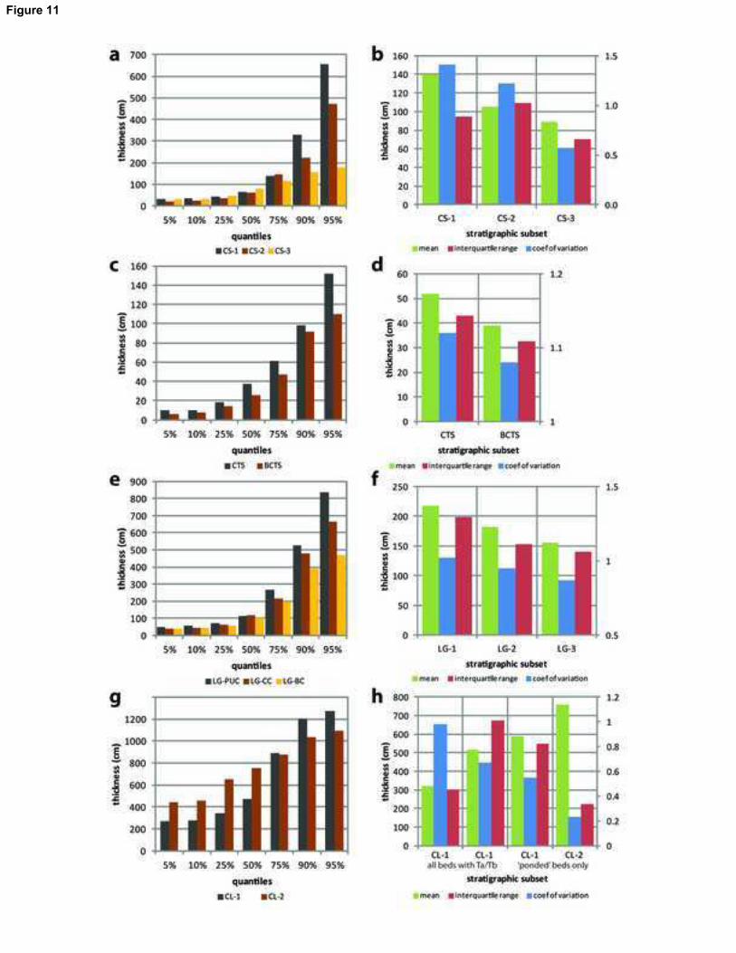
more likely to be confined by basin topography. Comparison of statistics (Fig. 11 and Table 3) of 690

the thick-bedded tails of different stratigraphic subsets of a case study highlights a coherent 691

modification of location and spread of the thickness population as a function of the degree of 692

ponding. This modification consists in a decrease of the thickness quantiles greater than 50% (i.e. 693

the median thickness) from older and more confined to younger and less confined stratigraphic 694

subsets (Figs. 11a, c, e, g). In all of the case studies except for the Cellino Formation, this results 695

in a likewise variation of mean, interquartile range and coefficient of variation values (Figs. 11b, d, 696

f, h). The departure of the Cellino Formation subsets from this behaviour may be because the 697

empirical samples are small (see Table 2) and include besides the ‘ponded’ beds, a significant but 698

stratigraphically variable proportion (from 60% in the lower E member to 40% in the upper E 699

member) of Bouma sequence turbidites. Restricting the treatment to ‘ponded’ beds only results 700

indeed in these statistics to conform to the aforesaid trend (Figs. 11h). In addition, it is not 701

surprising that the transition from the ponded to the partially ponded stage of the Castagnola 702

Formation is accompanied by a subtle but opposite variation of the interquartile range (Figs. 11b), 703

provided that the formulation of this statistical measure of dispersion does not account for either 704

28

extreme values nor normalization to the mean of a distribution. Another way to look at the 705

stratigraphic variability of thick-bedded tails is considering the high-end of both histograms and 706

exceedance probability plots (see paragraph 5) which, from more confined to less confined units of 707

the same case study, indicate a decrease in the frequency of thicker beds counterbalanced by an 708

increase in frequency of mid-range thicknesses. 709

In summary, the observed variability points to an overall reduction of ‘heaviness’ of the high-end 710

tail of thickness distributions (that is, how much it spreads toward high thickness values) from 711

ponded (e.g. CS-1, LG-1, CL-1) or partially ponded/more confined systems (e.g. CS-2, CTS and 712

LG-2) to less-confined (e.g. BCTS, CL-1) or unconfined systems (e.g. CS3 and LG-3) of the same 713

case study. It is suggested that sediment stripping and by-pass might represent the main controls 714

on the ‘heaviness’ of the thick-bedded tail of turbidite thickness distributions of partially ponded to 715

unconfined systems (see also paragraph 6.4 for additional discussion). 716

6.4. What model distribution best characterizes ponded turbidites? 717

If sampling biases were to be neglected, best-fitting results would suggest that, despite their 718

diverse depositional controls, the frequency distribution of turbidite thickness from any of the case 719

studies (‘all beds’ in Table 2) is reasonably well described with a log-normal model, though with 720

some stratigraphic variability in statistical location and dispersion of data. However, acknowledging 721

that a bias against very thin beds exists (see paragraphs 6.1-2) should lead to caution in drawing 722

such a conclusion, provided that commonly applied scaling laws (i.e. exponential, log-normal and 723

power-law) differ each from another in their low-end tail only (Talling, 2001; Sinlcair and Cowie, 724

2003; see also Cirillo, 2013). 725

As proposed in paragraph 6.3, a workaround to this problem is focusing on the thick bed 726

subpopulations which, though not very numerous, have been shown to be less affected by 727

sampling biases at the basin centre. If on one hand this approach may produce artificial truncation 728

of the low-end tail of the thickness population, on the other hand it has the advantage of restricting 729

29

the treatment to thick and laterally extensive turbidites deposited by large volume turbidity currents, 730

that is, to those beds more likely to yield a depositional signature of flow confinement. 731

Results of distribution fitting of the thick bed subpopulations (Table 2) suggest that while the 732

frequency distribution of thicknesses from ponded stratigraphic subsets (CS1, LG-1 and CL-1) is 733

better described by a power-law relationship, turbidite thickness data from partially ponded and 734

confined to unconfined units from the same case studies show a log-normal behaviour. Admittedly, 735

in most cases power-law and log normal models are very close best-fitting options (see Table 2), 736

suggesting they are both plausible and that, though intriguing, our results are not definitive and 737

need to be verified on larger thickness datasets via more refined approaches to goodness-of-fit 738

testing. However, whichever the best distribution model for thick bed subsets of our ponded to 739

partially ponded examples (i.e. power-law vs. log-normal with a high variance), the basin-wide 740

character of these beds would imply that the volume of the sandy part of turbidity currents reaching 741

the basin should scale linearly to turbidite thickness (Malinverno, 1997; Sinclair and Cowie, 2003) 742

thus showing a likewise frequency distribution. This observation has important implications in 743

prediction of net-to-gross in reservoir hosted in confined turbidite systems. Yet, it tells us little about 744

the frequency distribution of parent flow magnitude, whose assessment would require taking into 745

account the thickness of mud caps and is feasible only where there is a strong evidence of fully 746

ponded conditions. 747

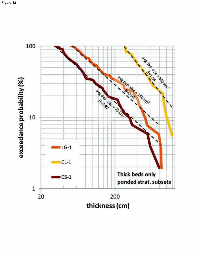
Should the power-law fit hold for the thick beds of our ponded to partially ponded examples, these 748

basin-wide beds would represent the megabeds of the Malinverno (1997) model, namely the 749

angular coefficient of the linear fits of Fig. 12 would represent くmega. However it is noteworthy that 750

there is some variability in the scaling exponent く from smaller to larger basin, with the ponded 751

examples from the Castangola and Laga formations (CS-1 and LG-1) showing similar values (く 752

≈0.95) much less than that of the power-law fit (く=1.54) of the Cellino Formation ponded subset 753

(CL-1). While the variability of く is in general agreement with trivial calculations of scaling of bed 754

volume to depocentre size, which predicts positive dependency of く on size of the basin given the 755

30

same power-law input signal (see Sinclair and Cowie, 2003), dividing its value by that by the 756

estimated average size of their host depocentre (Fig. 12) returns remarkably different values 757

ranging from 0.013 of CS-1 to 0.002 of CL-1. Also, it is unexpected finding that from smaller to 758

larger depocentre there is an increase in average thickness (Table 3), suggesting that, overall, the 759

thickness of these examples of ponded beds are positively related to depocentre size. There are 760

two alternative explanations for these results: i) if a frequency distribution of parent flow magnitude 761

with same scaling parameter く is to be assumed, our estimates of depocentre size might be 762

significantly inaccurate, or ii) both the scaling parameter く and average magnitude of the input 763

signal might be peculiar to each turbidite basin, e.g. depending on different dominant generative 764

process and flow types (see Talling 2015 for a review) and character and size of source areas. 765

Another interesting point highlighted by this study is that the ponded examples do not show any 766

evidence of three well-defined thickness subpopulations with power-law behaviour nor of the 767

corresponding gradients from くsmall to くlarge and くmega predicted by the Malinverno (1997) model. 768

Previously, Sylvester (2007) noted that the third segment くmega had never been reported in the 769

literature before his work, which in his view questions the possibility that the frequency distribution 770

of volumes of turbidity currents might follow a power-law scaling relationship. Only more recently 771

Felletti et al. (2009) and Felletti and Bersezio (2010) interpreted some cross-overs of the log-log 772

exceedance probability plot of turbidite thickness as the transition between the three 773

subpopulations of the Malinverno (1997) model but were not able to demonstrate the power-law 774

behaviour of any of these subpopulations. Also, as the transition between the subpopulations of 775

‘small’ and ‘large’ beds were coupled with a change in facies types, the changes in plot gradient 776

from くsmall to くlarge were interpreted by Felletti et al. (2009) and Felletti and Bersezio (2010) as 777

primarily reflecting rheology transitions in parent flows rather than undersampling of beds of 778

diameter smaller than the host basin radius. 779

However, reconsidering the assumptions of the Malinverno (1997) model, it must be noted that the 780

two power-law subpopulations of ‘small’ and ‘large’ beds as well as the flex separating them on a 781

log-log exceedance plot are not to be seen in the real world. This is because while the assumption 782

31

of a cylindrical shape holds for ‘ponded’ beds (being basin-wide the planform of ‘ponded’ beds can 783

be viewed as that of cylinder of diameter equal to that of the circular host basin) and will result in 784

linear scaling of thickness to bed volume, the three-dimensional shape of the deposit of non-785

ponded or unconfined flows cannot be assumed to be unique and adequately described by a 786

simple planform or scaling law of bed thickness to length and, therefore, the thickness of non-787

ponded beds might not follow a power-law frequency distribution even when volume of parent 788

flows do so. In conclusion, any analysis of turbidite thickness statistics to identify the signal of 789

basin confinement and flow ponding should be focused on the thick-bedded tail of the thickness 790

distribution rather than on fitting the distribution of the whole thickness range to result of numerical 791

models based on assumptions that might not be valid for the entire thickness range. 792

6.5. How is the initial bed thickness distribution modified by sediment by-pass? 793

What remains to be explored are the depositional controls behind the observed stratigraphic 794

modification in all of the case studies from high-variance thickness populations having thick-795

bedded tails with likely power-law behaviour to low-variance thickness populations characterized 796

by log-normal thick-bedded tails (Fig. 12 and 13). 797

Assuming that the input signal had not changed significantly over time, the plot of ponded subsets 798

can used as the initial best representation of input volumes. If we focus on thick-bedded tails only 799

for sake of better comparison (Fig. 13), this modification is expressed as an increase in the 800

upward-convexity of the exceedance probability plot from older and more confined to younger and 801

less confined stratigraphic subset. 802

Any explanation for the alterations of the initial thickness population shown in (Fig. 13) must 803

account for the different mechanics of flow spilling (Sinclair and Tomasso, 2002) of partially 804

ponded situations (e.g. CS-2 and LG-1 of the Castagnola and Laga formations) as opposed to 805

sediment by-pass (see Stevenson, 2015 for a review) of open-end confined and unconfined 806

turbidite systems. Also, it must take into consideration that, in ponded situations, the depocentre is 807

progressively enlarging as it is filled up with turbidites (e.g., stratigraphic transition from CS-1 to 808

32

CS-2 of the Castagnola Formation; see Table 1), which results in lateral shifting of the thickness 809

exceedance probability plot. 810

The idealized plot of Fig. 14 is an attempt to summarize the results of this study into a 811

comprehensive model tracking the likely modifications of the thickness frequency distribution of 812

turbidites that are initially ponded in an enclosed mini-basin at a measured location close to the 813

basin centre. As in the experiments of Malinverno (1997) and Sinclair and Cowie (2003), in initial 814

stage 1, as nearly all turbidites are ponded and basin-wide, bed geometry can be approximated 815

with cylindrical shapes of diameter equal to that of the depocentre. 816

The low-end of Fig. 14 plot below an arbitrary thickness of 20 cm is dashed showing that in stage 1 817

the initial frequency distribution of bed thickness (and that of magnitude of parent flows) below this 818

threshold is unknown, and it could have followed a power-law model or had a log-normal behaviour 819

and high-variance (Fig. 1). The plot focuses on how the initial thickness distribution is modified by 820

depositional controls rather than its character and meaning. Also, the effect of increase of 821

depocentre size is exaggerated to better visualize modifications of the initial distribution in four 822

stages, from 1 to 4. 823

In stage 2 of Fig. 14, the depocentre enlarges and the height of the confining topography reduces 824

as a consequence of sediment infilling (see Sinclair and Tomasso, 2002), There is an overall shift 825

of the plot toward the left, signifying an overall decrease in location and spread (i.e. mean, range 826

and variance) of the initial thickness frequency distribution and departure from its shape in both the 827

thin and the thick-bedded tails. The down bend of the low-end of the plot can be viewed as the 828

result of smaller flows being contained but not ponded by the depocentre topography: being their 829

volume much less than the receiving depocentre, smaller flows neither develop a ponded 830

character, nor deposit tabular basin-wide beds to be always intercepted in a section measured at 831

the basin centre. This effect entails a drop in the frequency of low-end thicknesses reflecting 832

undersampling of thin beds not reaching the measure location or too thin to be detected or 833

preserved (see paragraph 6.1) and a thickness cut-off (stars in Fig. 14), scaling to the minimum 834

33

volume of the flow able to develop a ponded character. This drop in the frequency distribution of 835

thin beds is that same modelled by Malinverno (1997), being the only difference that in the real 836

world, as these beds are not cylindrical but show diverse depositional shapes (and thickness 837

frequency distributions) reflecting flow rheology transitions, the thin-bedded segment is likely to 838

show a number of gradient changes (see e.g. Talling, 2001; Sylvester, 2007; Pantopoulos et al., 839

2013). The modification of the thick-bedded tail of stage 2 (Fig. 14) is interpreted as the result of 840

onset of flow stripping in partially ponded conditions, that is, the height of the confining topography 841

allows for some of the sand of the few largest flows to escape the basin spilling from a local sill. 842

Differently from sediment by-pass in unconfined settings, flow stripping is selective with respect to 843

flow magnitude (i.e. the amount of sediment escaping the basin is ultimately controlled the ratio of 844

thickness of the flow to height of the confining topography) which makes for a sharp gradient 845

change (circles in Fig. 14), or thickness cut-off, between the ‘ponded’ part of the plot and that 846

subject to modification. Overall the above mentioned modifications of the initial distribution results 847

in the plot of stage 2 showing a slightly convex-upward shape similar to that of empirical datasets 848

of CS-2 and LG-1, which both show a mild departure from the idealized plot of stage 1 in their thin 849

and thick-bedded tails (Fig. 14a, c). 850

In stage 3 (Fig. 14), the severity of modifications addressed for stage 2 is increased as a result of 851

the progress of depocentre infilling from turbidite. Is reasonable to assume that this might lead to 852

‘convergence’ of the thickness cut-offs of contained non-ponded turbidites and turbidites affected 853

by flow stripping (arrows in Fig. 14) with the end result of well-defined convex-upward shape of the 854

plot (e.g. LG-2; CL-2), which hints at a more that likely log-normality of the empirical distribution. 855

Such a ‘convergence’ involves that establishment of flow ponding and scaling of bed thickness to 856

parent flow volume is restricted to a progressively smaller range of flow magnitudes. 857

Stage 4 represents the situation where, further progression of depocentre evolution toward less 858

confined situations, results in conditions unfavourable to ponding whichever the flow magnitude. 859

The system is no longer ponded and none of the turbidite beds is basin-wide, therefore the 860

34

frequency distribution of turbidite thickness does not scale linearly to flow magnitude but must be 861

chiefly controlled by flow rheology, momentum and sediment by-pass. The model of stage 4 862

applies to all confined - non-ponded to unconfined examples of this study and is particularly well 863

expressed in the CTS and BCTS (Fig. 14b), where there is a strong independent evidence of flow 864

by-pass. 865

7. Conclusions 866

Aiming at assessing possible sampling biases and primary depositional control on turbidite 867

thickness statistics of confined basins, in this study we compared a number of thickness subsets 868

from four examples from the Central and Northern Apennine of Italy, which share a common 869

stratigraphic evolution from an early ponded to a late unconfined depositional setting. The core 870

finding of this research are as follows: 871

A sound assessment of likely sampling biases is key to correct interpretation of turbidite 872

thickness statistics, especially when spatial trends of bed thickness are documented. 873

Sampling biases are lowest when thicknesses are measured at the basin centre, 874

irrespective of the system internal architecture (basin-wide sheets pinching at basin 875

margins vs. laterally shifting lobes). 876

Stratigraphic variability in the studied succession should be accounted for by breaking 877

down thickness datasets into subsets with homogeneous sedimentological characteristics 878

in order to avoid a blurred statistical picture of turbidite thickness of little meaning for both 879

process sedimentology interpretations and bed volume prediction. 880

A bias against cm-thick Tc/Td Bouma sequence beds exists due to field operational 881

constraints, which can lead to significant modifications of the actual thickness frequency 882

distribution. 883

35

The beds with a basal Ta/Tb deposited by larger volume flows form a high-end tail of the 884

thickness population whose variance and frequency distribution bear some relationship to 885

degree of flow confinement. 886

Ponded examples where there is independent evidence of tabular basin-wide beds differ 887

from non-ponded to unconfined examples of the same case study for showing a high-end 888

tail of the thickness frequency distribution with higher variance and mean for which a 889

power-law scaling law cannot be excluded based on our data. 890

The frequency distribution of turbidite thicknesses measured at the basin centre in an 891

initially ponded mini-basin can be modified higher in the stratigraphy to a lower-variance 892

distribution because of flow-stripping and undersampling of thinner and laterally less 893

continuous beds deposited by small-volume as a result of enlargement of the host basin 894

and lowering of the height of the enclosing topography associated to basin infilling. 895

Acknowledgments 896

The Turbidites Research Group industry consortium (Anadarko, BG Group, BP, ConocoPhillips, 897

Dana Petroleum, Nexen, OMV, Petronas, Statoil, Tullow Oil and Woodside) is warmly 898

acknowledged for funding the research on the Castagnola Basin. Norske Shell AS and Statoil ASA 899

are acknowledged for financially supporting past research on the Laga Basin. We gratefully 900

acknowledge the reviewer George Pantopoulos for his constructive criticism and helpful comments 901

which helped improving the clarity of the manuscript. 902

References 903

Awadallah, S.A.M., Hiscott, R.N., Bidgood, M., Crowther, T. 2001. Turbidite facies and bed-904

thickness haracteristics inferred from microresistivity images of Lower to Upper Pliocene rift-905

basin deposits, Woodlark Basin, offshore Papua New Guinea Eds P. Huchon, B. Taylor, A. 906

Klaus, Proc. ODP, Sci. Results, 180, 1–30. 907

36

Baruffini, L., Cavalli, C., Papani, L. 1994. Detailed stratal correlation and stacking patterns of 908

the Gremiasco and lower Castagnola turbidite systems, Tertiary Piedmont Basin, northwestern 909

Italy. In: Weimer, P., Bouma, A.H., Perkins, B.F Eds 15th Annual Research Conference 910

Submarine Fans and Turbidite Systems , Society of Economic Palaeontologists and 911

Mineralogists, Gulf Coast Section, pp. 9-21. 912

Beattie, P.D., Dade, W.B., 1996. Is scaling in turbidite deposition consistent with forcing by 913

earthquakes?: Journal of Sedimentary Research, v. 66, p. 909-915. 914

Bersezio, R., Felletti, F., Micucci, L., 2005. Statistical analysis of stratal patterns and facies 915

changes at the terminations of ‘‘turbiditic’’ sandstone bodies: the Oligocene Cengio Unit 916

Tertiary Piedmont Basin. GeoActa 4, 83–104. 917

Bersezio, R., Felletti, F., Riva, R, Micucci, L., 2009. Trends in bed thickness and facies of 918

turbiditic sandstone bodies: unravelling the effects of basin confinement, depositional 919

processes and modes of sediment supply. In: Kneller, B., Martinsen, O.J., McCaffrey, B. Eds., 920

External Controls on Deep-Water Depositional Systems., vol. 92. SEPM Special Publications, 921

pp. 303–324. 922

Boccaletti, M., Calamita, F., Deiana, G., Gelati, R., Massari, F., Moratti, G., Ricci Lucchi, F., 923

1990. Migrating foredeep-thrust belt system in the northern Apennines and Southern Alps. 924

Palaeogeography, Palaeoclimatology, Palaeoecology 77, 3–14. 925

Bouma, A.H. 1962. Sedimentology of Some Flysch Deposits; A Graphic Approach to Facies 926

Interpretation. Elsevier, Amsterdam, New York, 168 pp. 927

Carlson, J., Grotzinger, J.P., 2001. Submarine fan environment inferred from turbidite thickness 928

distribution: Sedimentology, v. 48, p. 1331-1351. 929

Carminati, E., Doglioni, C., 2012. Alps vs. Apennines: The paradigm of a tectonically 930

asymmetric Earth. Earth-Science Reviews 112 2012 67–96 931

37

Carruba, S., Casnedi, R., Felletti, F. 2004. From seismic to bed: surface–subsurface 932

correlations within the turbiditic Cellino Formation central Italy.Petroleum Geoscience, 102, 933

131-140. 934

Carruba, S., Casnedi, R., Perotti, C. R., Tornaghi, M., Bolis, G. 2006. Tectonic and 935

sedimentary evolution of the Lower Pliocene Periadriatic foredeep in Central Italy. International 936

Journal of Earth Sciences, 954, 665-683. 937

Casnedi, R., 1983. Hydrocarbon-bearing submarine fan system of Cellino Formation, Central 938

Italy: American Association of Petroleum Geologists Bulletin, v. 67, p. 359–370. 939

Casnedi, R., Follador, U., Moruzzi G., 1976. Geologia del campo gassifero di Cellino Abruzzo: 940

Bollettino della Società Geologica Italiana, v. 95, p. 891-901. 941

Cavanna, F., Di Giulio, A., Galbiati, B., Mosna, S., Perotti, C. R. Pieri, M. 1989. Carta geologica 942

dell'estremità orientale del Bacino Terziario Ligure-Piemontese. Atti Ticinesi di Scienze della 943

Terra, 32. 944

Cazzola, C., Fonnesu, F., Mutti, E., Rampone, G., Sonnino, M., Vigna, B., 1981. Geometry and 945

facies of small, fault-controlled deep-sea fan systems in a transgressive depositional setting. In: 946

Ricci Lucchi, F. Ed.. IAS – 2nd European Regional Meeting Excursion Guidebook, Bologna, pp. 947

7–53 Tertiary Piedmont Basin, northwestern Italy. 948

Cazzola, C., Mutti, E., Vigna, B., 1985. Cengio Turbidite System, Italy. In: Bouma, A., Normark, 949

W.R., Barnes, N.E. Eds., Submarine Fans and Related Turbidite Systems. Springer Verlag, pp. 950

179–183. 951

Centamore, E., Chiocchini, U., Cipriani, N., Deiana, G., Micarelli, A. 1978. Analisi 952

dell’evoluzione tettonico-sedimentaria dei “bacini minori” torbiditici del Miocene medio-953

superiore nell’Appennino umbro-marchigiano e laziale-abruzzese: 5) risultati degli studi in 954

corso. Memorie della Società Geologica Italiana, 18, 135-170. 955

38

Chen, C., Hiscott, R.N., 1999. Statistical analysis of facies clustering in submarine-fan turbidite 956

successions. J. Sediment. Res. 69, 505–517. 957

Cirillo, P. 2013. Are your data really Pareto distributed?. Physica A: Statistical Mechanics and 958

its Applications, 39223, 5947-5962. 959

Clauset, A., Shalizi, C. R., Newman, M. E. 2009. Power-law distributions in empirical 960

data. SIAM review, 514, 661-703. 961

Di Giulio, A., Galbiati, B. 1998. Turbidite record of the motions along a crustal-scale tectonic 962

line:the motions of the Villarvernia-Varzi line during the Oligocene-Miocene North-Western 963

Italy. In: 15th Internetional Sedimentological Congress, pp. 293-294. IAS - Universidad de 964

Alicante, Alicante, Spain. 965

Doglioni, C., 1991. A proposal of kinematic modelling for W-dipping subductions – possible 966

applications to the Tyrrhenian–Apennines system. Terra Nova 3, 423–434 967

Drummond C.N., 1999. Bed-thickness structure of multi-sourced ramp turbidites: Devonian 968

Brailler formation, Central Appalachian Basin: Journal of Sedimentary Research, v. 69, p. 115-969

121. 970

Drummond, C.N. and Wilkinson, B.H., 1996. Stratal Thickness Frequencies and the 971

Prevalence of Orderedness in Stratigraphic Sequences: Journal of Geology, v.104, p. 1-18. 972

Felletti F., Carruba S. and Casnedi R. 2009. Sustained turbidity currents: evidence from the 973

Pliocene Periadriatic foredeep Cellino Basin, Central Italy. In Kneller, B., Martinsen, O.J., and 974

McCaffrey, B., eds., External Controls on Deep-Water Depositional Systems: SEPM Special 975

Publication 92, 325-346. 976

Felletti, F., 2002. Complex bedding geometries and facies associations of the turbiditic fill of a 977

confined basin in a transpressive setting (Castagnola Formation, Tertiary Piedmont Basin, NW 978

Italy). Sedimentology 49, 645–667. 979

39

Felletti, F. 2016. Depositional architecture of a confined, sand-rich submarine system: the Bric 980

la Croce – Castelnuovo turbidite system (Tertiary Piedmont Basin, Oligocene, NW Italy). Italian 981

Journal of Geoscience, 134 (2015). DOI: 10.3301/IJG.2015.15 982

Felletti, F., Bersezio, R., 2010. Quantification of the degree of confinement of a turbidite-filled 983

basin: a statistical approach based on bed thickness distribution. Mar. Pet. Geol. 27, 515e532. 984

Flint, S.,Bryant, I.D. 1993. The geological modelling of hydrocarbon reservoirs and outcrop 985

analogues. Int. Assoc. Sedimentol. Spec. Publ., 15, 269 pp. 986

Gelati, R., Gnaccolini, M., 1980. Significato dei corpi arenacei di conoide sottomarina 987

Oligocene–Miocene inferiore nell’evoluzione tettonico-sedimentaria del Bacino Terziario 988

Ligure-Piemontese. Rivista Italiana di Paleontologia e Stratigrafia 87, 167–186. 989

Gelati, R., Gnaccolini, M., 1998. Synsedimentary tectonics and sedimentation in the Tertiary 990

Piedmont Basin, Northwestern Italy. Rivista Italiana di Paleontologia e Stratigrafia 98, 425–452. 991

Ghibaudo, G., Massari, F., Chiambretti, I., d’Atri, A., 2014a. Oligo-Miocene tectono-992

sedimentary evolution of the Tertiary Piedmont Basin southern margin, Roccaverano area-993

Langhe sub-basin NW Italy. Journal of Mediterranena Earth Sciences, 6, 1-51. 994

Ghibaudo, G., Massari, F., Chiambretti, I., 2014b. Oligo-Miocene tectono-sedimentary 995

evolution of the Langhe sub-basin: from continental to basinal setting Tertiary Piedmeont Basin 996

– Northwestern Italy. Journal of Mediterranean Earth Sciences, 6, 53-144. 997

Goldstein, M.L., Morris, S.A., Yen, G.G. 2004. Problems with fitting to the power law 998

distribution. Eur. Phys. J. B, 41, 255–258. 999

Haughton, P.D.W., 1994. Deposits of Deflected and Ponded Turbidity Currents, Sorbas Basin, 1000

Southeast Spain. Journal of Sedimentary Research Section, 642, 233-246.DOI: 1001

10.1306/D4267D6B-2B26-11D7-8648000102C1865D 1002

40

Haughton, P., Davis, C., McCaffrey, W., Barker, S., 2009. Hybrid sediment gravity flow 1003

deposits - Classification, origin and significance. Marine and Petroleum Geology, 2610, 1900-1004

1918. DOI:10.1016/j.marpetgeo.2009.02.012 Hiscott, R. N.; Colella, A.; Pezard, P.; Lovell, M. 1005

A.;Malinverno, A. 1992. Sedimentology of deep-water volcaniclastics, Oligocene Izu-Bonin 1006

forearc basin, based on formation microscanner images. In Taylor, B., Fujioka, K., eds. Proc. 1007

Ocean Drilling Project, Scientific Results 126:75-96. 1008

Hiscott, R.N., Colella, A., Pezard, P., Lovell, M.A., Malinverno, A., 1993. Basin plain turbidite 1009

succession of the Oligocene Izu-Bonin intraoceanic forearc basin. Mar. Petrol. Geol., 10, 450–466. 1010

Isaaks, E. H.,Srivastava, R. M. 1989. Applied Geostatistics, 561 pp. 1011

Janocko, M., 2010. Pinchout Geometry of Sheet-like Sandstone Beds: a new statistical 1012

approach to the problem of lateral bed thinning based on outcrop measurements. Lambert 1013

Academic Publishing. 978-3843380317. 1014

Kolmogorov, A.N., 1951. Solution of a problem in probability theory connected with the problem 1015

of the mechanics of stratification. Ann. Maths Soc. Trans., 53, 171–177. 1016

Kneller, B., McCaffrey, W., 1999. Depositional effects of flow nonuniformity and stratification 1017

within turbidity currents approaching a bounding slope; deflection, reflection, and facies 1018

variation. Journal of Sedimentary Research 695: 980-991. 1019

Kneller, B.C., McCaffrey, W., 1999. Depositional effects of flow non-uniformity and stratification 1020

within turbidity currents approaching a bounding slope. Deflection, reflection and facies 1021

variation. J. Sediment. Res. 69, 980–991. 1022

Lomas, S.A., Joseph, P., 2004. Confined turbidite systems. In: Lomas, S.A., Joseph, P. Eds., 1023

Confined Turbidite Systems. Geological Society, vol. 222. Special Publications, London, pp. 1–1024

7. 1025

41

Lowe, D. R. 1982. Sediment gravity flows: II Depositional models with special reference to the 1026

deposits of high-density turbidity currents. Journal of Sedimentary Research, 521. 1027

Maino M., Decarlis A., Felletti F., Seno. S. 2013 – Tectono-sedimentary evolution of the 1028

Tertiary Piedmont Basin NW Italy within the Oligo–Miocene central Mediterranean 1029

geodynamics. Tectonics, Vol. 32, pp.1–27, doi:10.1002/tect.20047. 1030

Manzi V., Lugli S., Ricci Lucchi F.,Roveri M. 2005 - Deep-water clastic evaporites deposition in 1031

the Messinian Adriatic foredeep Northern Apennines, Italy: did the Mediterranean ever dry 1032

out?. Sedimentology, 52, 875-902.Malinverno A., 1997, On the power-law distribution of 1033

turbidite beds: Basin Research. v. 9, p. 263-274. 1034

Malinverno, A.,Ryan, W. B. 1986. Extension in the Tyrrhenian Sea and shortening in the 1035

Apennines as result of arc migration driven by sinking of the lithosphere. Tectonics, 52, 227-1036

245. 1037

Marini, M. Milli, S. Ravnås, R., Moscatelli, M. 2015. A comparative study of confined vs. semi-1038

confined turbidite lobes from the Lower Messinian Laga Basin Central Apennines, Italy: 1039

Implications for assessment of reservoir architecture. Marine and Petroleum Geology 63, 142-1040

165 1041

Marini, M., Patacci, M., Felletti, F.,McCaffrey, W. D. 2016. Fill to spill stratigraphic evolution of a 1042

confined turbidite mini-basin succession, and its likely well bore expression: The Castagnola 1043

Fm, NW Italy. Marine and Petroleum Geology, 69, 94-111. 1044

McBride, E. F. 1962. Flysch and associated beds of the Martinsburg Formation Ordovician, 1045

Central Appa-lachians. J. Sediment. Petrol. 32:39-91. 1046

Milli, S., Moscatelli, M., Stanzione, O., Falcini, F., 2007. Sedimentology and physical 1047

stratigraphy of the Messinian turbidite deposits of the Laga basin central Apennines, Italy. Boll. 1048

Soc. Geol. Ital. 126, 255-281. 1049

42

Milli, S., Moscatelli, M., Marini, M., Stanzione, O., 2009. The Messinian turbidites deposits of 1050

the Laga Basin Central Apennines, Italy. In: Northern and Central Apennines Turbidites Italy 1051

Edited By Tinterri R., Muzzi Magalhaes P., Milli S., Marini M., Moscatelli M., Stanzione O., Field 1052

Trip 12, 27th Ias Meeting 24-28 September 2009, Alghero, Italy, 35-54. ISBN 978-88-6025-1053

123-7. 1054

Milli, S., Cannata, D., Marini, M., Moscatelli, M., 2013. Facies and geometries of Lower 1055

Messinian Laga Basin turbidite deposits central Apennines, Italy. In: Milli S., Brandano M. Eds., 1056

Excursion Guidebook, post-congress field trip of the XI GeoSed congress, September 26-28, 1057

2013. Journal of Mediterranean Earth Sciences, 5, 179-225. 1058

Mizutani, S., Hattori, I. 1972 Stochastic analysis of bed thickness distribution of sediments. 1059

Math. Geol., 4, 123– 146. 1060

Murray, C.J., Lowe, D.R., Graham, S.A., Martinez, P.A., Zeng, J., Carroll, A., Cox, R., Hendrix, 1061

M., Heubeck, C., Miller, D., Moxon, I.W., Sobel, E., Wendebourg, J., Williams, T., 1996. 1062

Statistical analysis of bed-thickness patterns in a turbidite section from the Great Valley 1063

Sequence, Cache Creek California. J. Sediment. Petrol 66, 900–908. 1064

Mosca P., Polino R, Rogledi S., Rossi M. 2010. New data for the kinematic interpretation of the 1065

Alps–Apennines junction Northwestern Italy, Int J Earth Sci Geol Rundsch, V. 99, pp 833–849 1066

Muto, T. 1995 The Kolmogorov model of bed-thickness distribution: an assessment based on 1067

numerical simulation and field data analysis. Terra Nova, 7, 417–423. 1068

Mutti, E. 1992. Turbidite sandstones. Agip, Istituto di geologia, Università di Parma. 1069

Mutti, E., Sonnino, M., 1981. Compensation cycles: a diagnostic feature of turbidite sandstone 1070

lobes, in: IAS Eur. Reg. Meeting, Bologna, Vol. Abstract II. 1071

43

Pantopoulos, G., Vakalas, I., Maravelis, A., Zelilidis, A. 2013. Statistical analysis of turbidite 1072

bed thickness patterns from the Alpine fold and thrust belt of western and southeastern 1073

Greece. Sedimentary Geology, 294, 37-57. 1074

Patacci, M., Haughton, P. D. W., McCaffrey, W. D. 2015. Flow Behavior of Ponded Turbidity 1075

Currents. Journal of Sedimentary Research 858: 885-902. 1076

Patacci, M. 2016. A high-precision Jacob's staff with improved spatial accuracy and laser 1077

sighting capability. Sedimentary Geology 335: 66-69. 1078

Pickering, K. T.,Hiscott, R. N. 1985. Contained reflected turbidity currents from the Middle 1079

Ordovician Cloridorme Formation, Quebec, Canada: an alternative to the antidune 1080

hypothesis. Sedimentology, 323, 373-394. 1081

Pickering, K. T.,Hiscott, R. N., 2015. Deep marine systems: processes, deposits, 1082

environments, tectonics and sedimentation. John Wiley & Sons, 23 Oct 2015, 672 pp. 1083

Prather, B. E., Pirmez, C., Winker, C. D. 2012. Stratigraphy of linked intraslope basins: Brazos-1084

Trinity System, western Gulf of Mexico.Application of the Principles of Seismic Geomorphology 1085

to Continental-Slope and Base-of-Slope Systems: Case Studies from Seafloor and Near-1086

Seafloor Analogues: SEPM Special Publication, 99, 83-109. 1087

Prélat, A., Hodgson, D. M. 2013. The full range of turbidite bed thickness patterns in submarine 1088

lobes: controls and implications. Journal of the Geological Society, 1701, 209-214. 1089

Ravnås, R., Steel, R. J. 1997. Contrasting styles of Late Jurassic syn-rift turbidite 1090

sedimentation: a comparative study of the Magnus and Oseberg areas, northern North 1091

Sea. Marine and Petroleum Geology, 144, 417-449. 1092

Ravnås, R., Nøttvedt, A., Steel, R. J., Windelstad, J. 2000. Syn-rift sedimentary architectures in 1093

the Northern North Sea. Geological Society, London, Special Publications, 1671, 133-177. 1094

44

Remacha, E., Fernández, L. P., Maestro, E. 2005. The transition between sheet-like lobe and 1095

basin-plain turbidites in the Hecho basin south-central Pyrenees, Spain. Journal of 1096

Sedimentary Research, 755, 798-819. 1097

Ricci Lucchi, F. 1969. Channelized deposits in the middle Miocene flysch of Romagna Italy. 1098

Museo Geologico "Giovanni Capellini". 1099

Ricci Lucchi, F., 1986, The Oligocene to Recent foreland basins of the northern Apennines: in 1100

Allen, P.,A., Homewood, P., eds, Foreland Basins Sp. Publ. of the IAS, v. 8, p. 105-139. 1101

Ricci Lucchi, F. Valmori, E. 1980. BasinǦwide turbidites in a Miocene, overǦsupplied deepǦsea 1102

plain: a geometrical analysis. Sedimentology, 273, 241-270. 1103

Rothman, D.H., Grotzinger, J.P. 1996 Scaling properties of gravity-driven sediments. Nonlinear 1104

Processes Geophys., 2, 178–185. 1105

Rothman, D.H., Grotzinger, J.P., Flemings, P., 1994, Scaling in turbidite deposition: Journal of 1106

Sedimentary Research, v. 24, p. 59-67. 1107

Sinclair, H. D. 1994. The influence of lateral basinal slopes on turbidite sedimentation in the 1108

Annot sandstones of SE France. Journal of Sedimentary Research, 641. 1109

Sinclair, H. D., Tomasso, M. 2002. Depositional evolution of confined turbidite basins. J. 1110

Sediment. Res. 72:451-456. 1111

Sinclair, H.D. Cowie, P.A. 2003 Basin-Floor Topography and the Scaling of Turbidites. J. Geol., 1112

111, 277–299. 1113

Southern, S. J., Patacci, M., Felletti, F. McCaffrey, W. D. 2015. Influence of flow containment 1114

and substrate entrainment upon sandy hybrid event beds containing a co-genetic mud-clast-1115

rich division. Sedimentary Geology 321: 105-122. 1116

45

Stevenson, C. J., Jackson, C. A. L., Hodgson, D. M., Hubbard, S. M., Eggenhuisen, J. T. 2015. 1117

Deep-water sediment bypass. Journal of Sedimentary Research, 859, 1058-1081. 1118

Stocchi, S., Cavalli, C. Baruffini, L. 1992 I depositi torbiditici di Guaso Pirenei centro 1119

meridionali, Gremiasco e Castagnola settore orientale del BTP: geometria e correlazioni di 1120

dettaglio. Atti Ticinensi Scienze della Terra, 35, 154-177. 1121

Stuart, A., 1962, Basic Ideas of Scientific Sampling, Hafner Publishing Company, New York. 1122

Sylvester, Z., 2007, Turbidite bed thickness distributions: methods and pitfalls of analysis and 1123

modelling: Sedimentology, v. 54, p. 847–870. 1124

Talling P., 2001, On the frequency distribution of turbidite thickness: Sedimentology, v. 48, p. 1125

1297-1329. 1126

Talling, P.J., 2013. Hybrid submarine flows comprising turbidity current and cohesive debris 1127

flow: deposits, theoretical and experimental analyses, and generalized models. Geosphere 9, 1128

460–488. 1129

Talling, P.J., Amy, L.A.,Wynn, R.B., Peakall, J., Robinson, M., 2004. Beds comprising debrite 1130

sandwiched within co-genetic turbidite: origin and widespread occurrence in distal depositional 1131

environments. Sedimentology 51, 163–194. 1132

Tinterri, R. 2011. Combined flow sedimentary structures and the genetic link between 1133

sigmoidal-and hummocky-cross stratification.GeoActa, 104. 1134

Tinterri, R., Tagliaferri, A. 2015. The syntectonic evolution of foredeep turbidites related to 1135

basin segmentation: Facies response to the increase in tectonic confinement Marnoso-1136

arenacea Formation, Miocene, Northern Apennines, Italy. Marine and Petroleum Geology, 67, 1137

81-110. 1138

Lamb, M. P., Toniolo, H., Parker, G. 2006. Trapping of sustained turbidity currents by 1139

intraslope minibasins. Sedimentology, 531, 147-160. 1140

46

Turcotte, D. L. 1997. Fractals and chaos in geology and geophysics. Cambridge, Cambridge 1141

University Press, 397 p. 1142

Vai, G.B. 2001 Structure and stratigraphy: an overview. In Vai, G.B., Martini, I.P. eds Anatomy 1143

of an Orogen: the Apennines and Adjacent Mediterranean Basin, Kluwer Dordrecht, p.p. 15-32. 1144

Van Andel, T. H., D Komar, P.. 1969. Ponded sediments of the Mid-Atlantic Ridge between 22 1145

and 23 north latitude. Geological Society of America Bulletin, 807, 1163-1190. 1146

Vezzani, L., Casnedi, R., Ghisetti, F., 1993, Geological map of the north-eastern Abruzzo 1147

region. Scale 1:100.000: S.EL.CA, Firenze. 1148

Wheatcroft, R. A. 1990. Preservation potential of sedimentary event layers.Geology, 189, 843-1149

845. 1150

Figure and table captions 1151

1152

Table 1. Main characteristics of the case studies included in this work, compiled and partially 1153

revised from literature (see bottom row). 1154

Table 2. Likely parent distributions for stratigraphic and bed type subsets with estimated 1155

parameters and results (rounded to two decimal places) of the Anderson-Darling (A-D) and 1156

Chi-Squared (Chi-Sq) goodness of fit tests. Thick marks in right-hand size of test statistics 1157

columns indicate that the model distribution passes the test with a significance level of 1158

0.1whereas x indicate its rejection. ‘Tc/Td base’ and ‘Ta/Tb base’ bed type subsets are rippled 1159

to parallel laminated beds (i.e. Tc-d Bouma sequences) and beds starting with a massive or 1160

planar-parallel laminate division (i.e. Ta/Tb Bouma division). 1161

Table 3. Descriptive statistics quantifying variability and location of the right thick-bedded tails 1162

of stratigraphic subsets from the case studies. 1163

47

Figure 1. Log-log plot of thickness exceedance probabilities contrasting most commonly used 1164

model distributions for turbidite thicknesses: (1) power-law, (2) exponential and (3) low-1165

variance log-normal and (4) high-variance log-normal model distributions. Note how the thick-1166

bedded tails (right side of the plot) of 2 and 4 behave similarly to that of 3 and 1, respectively, 1167

making unpractical to distinguish between alternative model distributions when detailed data 1168

from the thin-bedded tail are not available. 1169

Figure 2. Numerical experiments on turbidite thickness statistics of confined basins: (a) 1170

‘segmented’ distribution of turbidite thicknesses measured at the centre of a circular basin 1171

produced using the assumptions of the ‘confined basin model’ of Malinverno (1997) 1172

(experiment 1, modified after Sylvester, 2007); (b) effects of (2) flow ponding and (3) flow 1173

stripping on thickness distributions of turbidites deposited in an enclosed circular basin by 1174

inbound flows with power-law volume distribution (1) (modified, after Sinclair and Cowie, 2003). 1175

See paragraph 2.1 for details and explanation. 1176

Figure 3. Simplified sketch showing the eastward migration of the Apennine foredeep from 1177

Oligocene to present. Bold letters indicate turbidite infill of small, confined wedge top basins 1178

(L= Laga Basin; C= Cellino Basin). Modified after Di Biase and Mutti, 2002. 1179

Figure 4. (a) Stratigraphic framework and (b) present-day layout of the Tertiary Piedmont 1180

Basin. Modified after Mosca et al. (2010). 1181

Figure 5. (a) Stratigraphic framework of the Upper Miocene to Pleistocene deposits of the 1182

Laga Basin and the Periadriatic foreland system (modified after Carruba et al. 2006). Studied 1183

units in bold; (b) Simplified geological map of the Laga Formation and Cellino Formation 1184

outcrops with location of the composite sections from which thickness data were taken. 1185

Figure 6. Bi-logarithmic thickness exceedance probability (as percent) plots showing a) the 1186

frequency distributions of turbidites from the individual stratigraphic units (CS-1, CS-2 and CS-1187

3) of the Castagnola Formation (CS) besides that of the whole CS dataset (CS-1-3); b) the 1188

48

variability of the measured thickness distributions of a confined sheet-like turbidite package 1189

(Crognaleto lobe complex, Laga Formation) resulting from moving the measure location from 1190

the basin axis toward the lateral basinal slope; c) the variability of the measured thickness 1191

distributions of a package of turbidite lobes with compensational stacking (Mt. Bilanciere 1192

complex, Laga Formation) resulting from moving laterally the measure location; the effect of 1193

undersampling of cm-thick beds assuming CS-1 (black line) as the actual bed thickness 1194

population (d) or (e) acknowledging that 150 beds thinner than 10 cm may have been not 1195

measured in the field. See text for explanation. 1196

Figure 7. Turbidite thicknesses from the Castagnola Formation: (a), (b) and (c) are log-log 1197

exceedance probability plots of turbidite sandstone thicknesses from unit 1 to 3 with breakdown 1198

into bed type subsets; (d) is a histogram plotting the binned bed thicknesses, with the labels 1199

indicating the upper value of the bin interval, versus their relative frequency (logarithmic scale). 1200

Figure 8. Turbidite thicknesses from the Cengio (CTS) and Bric la Croce-Castelnuovo 1201

Turbidite Systems (BCTS): (a) and (b) are log-log exceedance probability plots of turbidite 1202

sandstone thicknesses of CTS and BCTS, respectively, with breakdown into bed type subsets; 1203

(d) is a histogram plotting the binned bed thicknesses, with the labels indicating the upper 1204

value of the bin interval, versus their relative frequency (logarithmic scale). 1205

Figure 9. Turbidite thicknesses from the lower Laga Formation lobes: (a), (b) and (c) log-log 1206

exceedance probability plots of turbidite sandstone thicknesses from the Poggioumbricchio 1207

(LG-1), the Crognaleto (LG-2) and the Mt. Bilanciere (LG-3) lobe complexes, respectively, with 1208

breakdown into bed type subsets; (d) histogram plotting bed thicknesses, with the labels 1209

indicating the upper value of the bin intervals, versus their relative frequency (logarithmic 1210

scale). 1211

Figure 10. Turbidite thicknesses from the E member of the Cellino Formation: (a), (b) log-log 1212

exceedance probability plots of turbidite sandstone thicknesses from the lower (CL-1) and 1213

49

more confined and the upper and less confined (CL-2) parts of the E member with breakdown 1214

into bed type subsets; c) detail showing the mixing of two further bed type subpopulation in the 1215

thin-bedded tail of CL-1; (d) histogram plotting bed thicknesses, with the labels indicating the 1216

upper value of the bin interval, versus their relative frequency (logarithmic scale). 1217

Figure 11. Bar-charts of thickness quantiles (a, c and e, left-hand side) and mean, interquartile 1218

range (primary axes, in m) and coefficient of variation (dimensionless, on secondary axes) (b, 1219

d, and f, right-hand side) quantifying location and spread of the thick-bedded tail of stratigraphic 1220

subsets from (top to bottom) the Castagnola Formation, the Cengio-Bric la Croce-Castelnuovo 1221

Turbidite Systems, the Laga Formation lobes and E member of the Cellino Formation 1222

Figure 12. Log-Log thickness exceedance probability plot comparing the thick-bed 1223

subpopulations of ponded examples from the Castagnola Formation (CS-1) Laga (LG-1) and 1224

Cellino (CL-1) formations. Note how the scaling parameter く increases from smaller to larger 1225

host depocentres in agreement with the model of Sinclair and Cowie (2003). Dashed lines are 1226

power-law best-fits of Table 2 noted with average estimated sizes of host depocentres. 1227

Figure 13. Log-Log thickness exceedance probability plots comparing the frequency 1228

distributions of thick-bedded tails of stratigraphic subsets with different depositional controls 1229

(see legend) from: a) the Castagnola Formation, b) the Cengio-Bric la croce-Castelnuovo 1230

Turbidite systems, c) Laga Formation lobes and d) Cellino Formation Note how there is a 1231

tendency from more confined to less confined subsets to an increase in the overall upward-1232

convexity of the plots relating to modification of shape and spread of thickness frequency 1233

distributions. 1234

Figure 14. Log-Log thickness exceedance probability (as number of beds) plots showing the 1235

modifications affecting the empirical distribution of turbidite thicknesses at the basin centre of 1236

an enclosed ponded mini-basin were all of the turbidity currents are initially ponded (stage 1). 1237

Stage 2 and 3 illustrate the effect on the initial thickness distribution of progressive 1238

50

enlargement of the depocentre and reduction of height of the confining topography with 1239

ongoing sediment infilling, resulting in smaller flows being no longer ponded by topography and 1240

few largest flows undergoing flow stripping. Stage 4 represents the final result of basin 1241

topography evolution, namely the onset of contained non-ponded or even unconfined 1242

conditions. 1243

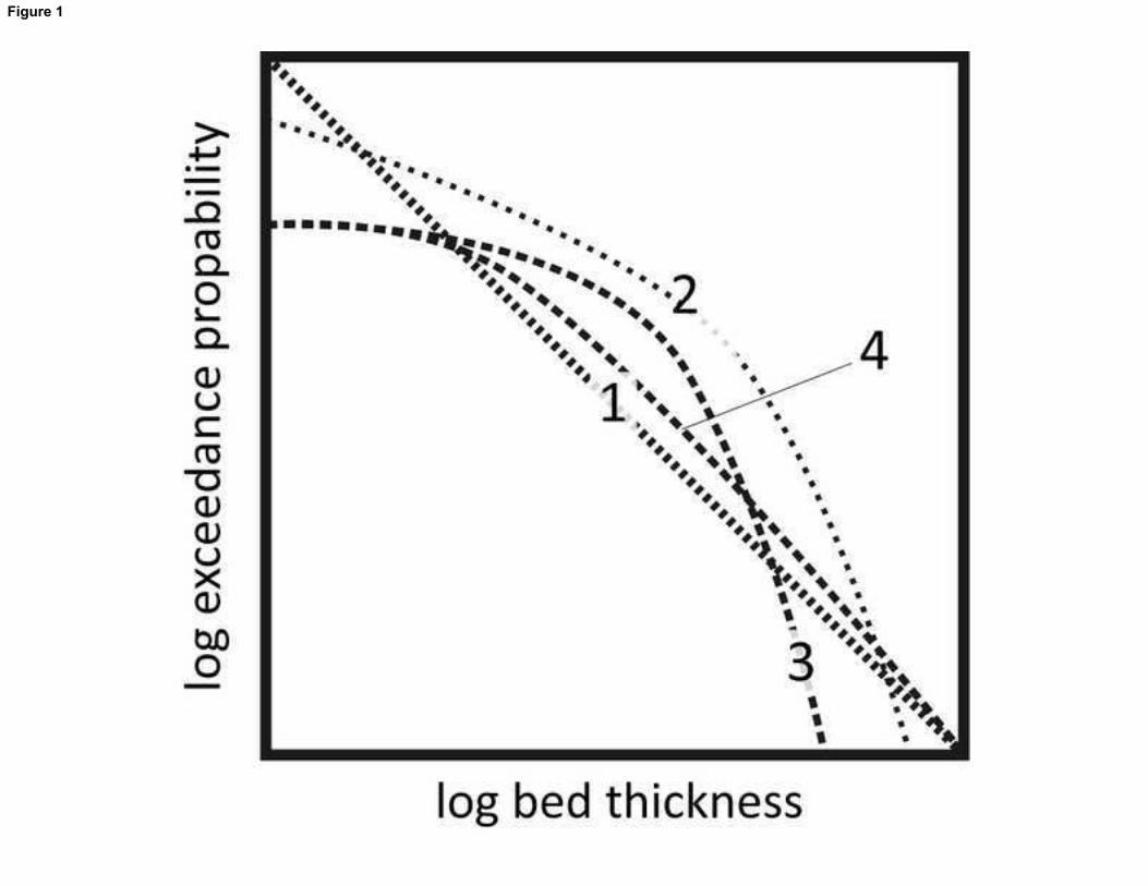
Figure 1

Figure 2

Figure 3

Figure 4

Figure 5

Figure 6

Figure 7

Figure 8

Figure 9

Figure 10

Figure 11

Figure 12

Figure 13

Figure 14

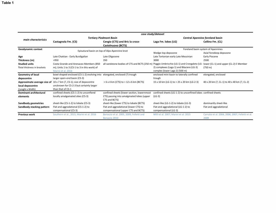
Castagnola Fm. (CS) Cengio (CTS) and Bric la croce-

Castelnuovo (BCTS)

Laga Fm. lobes (LG) Cellino Fm. (CL)

Wedge-top depozone Axial foredeep depozone

Age Late Chattian - Early Burdigalian Late Oligocene Late Tortonian-early Late Messinian Early Piocene

Thickness (m) >950 350 3000 2500

Studied units

Total thickness in brackets

Costa Grande and Arenaceo Members (850

m); Units 1 to 3 (CS-1 to 3 in this work) of

Marini et al. 2016

all sandstone bodies of CTS and BCTS (250 m) Poggio Umbricchio (LG-1) and Crongaleto (LG-

2) complexes (Laga 1) and Bilaciere (LG-3)

complex (lower Laga 2) (500 m)

lower (CL-1) and upper (CL-2) E Member

(750 m)

Geometry of local

depocentre

bowl-shaped enclosed (CS-1-2) evolving into

larger open-end basin (CS-3)

elongated, enclosed (?) trough enclosed mini-basin to laterally confined

trough

elongated, enclosed

Approximate average size of

local depocentre

(Lenght x Width)

10 x 7 km (?, CS-1); size of depocentre

uncknown for CS-2-3 but certainly larger

than that of CS-1

> 6 x 4 km (CTS) to > 12 x 6 km (BCTS) 15 x 10 km (LG-1) to > 25 x 20 km (LG-2-3) 40 x 20 km (?, CL-1) to 40 x 40 km (?, CL-2)

Dominant architectural

elements

confined sheets (CS-1-2) to unconfiend

locally amalgamated obes (CS-3)

confined sheets (lower section, lowernmost

CTS) passing into amalgmated lobes (upper

CTS and BCTS)

confined sheets (LG-1-2) to unconfined lobes

(LG-3)

confined sheets

Sandbody geometries sheet-like (CS-1-2) to lobate (CS-3) sheet-like (lower CTS) to lobate (BCTS) sheet-like (LG-1-2) to lobate (LG-3) dominantly sheet-like

Sandbody stacking pattern Flat and aggradational (CS-1-2) to

compensational (CS-3)

Flat and aggradational (lower CTS) to

compensational (upper CTS and BCTS)

Flat and aggradational (LG-1-2) to

compensational (LG-3)

Flat and aggradational

Previous work Southern et al., 2015; Marini et al. 2016 Bersezio et al. 2005, 2009; Felletti and

Bersezio 2010

Milli et al. 2007; Marini et al. 2015 Carruba et al. 2004, 2006, 2007; Felletti et al.

2009

main characterisics

case study/dataset

Central Apennine foreland basin

Geodynamic context Foreland basin system of Apennines

Tertiary Piedmont Basin

Episutural basin on top of Alps-Apennine knot

Table 1

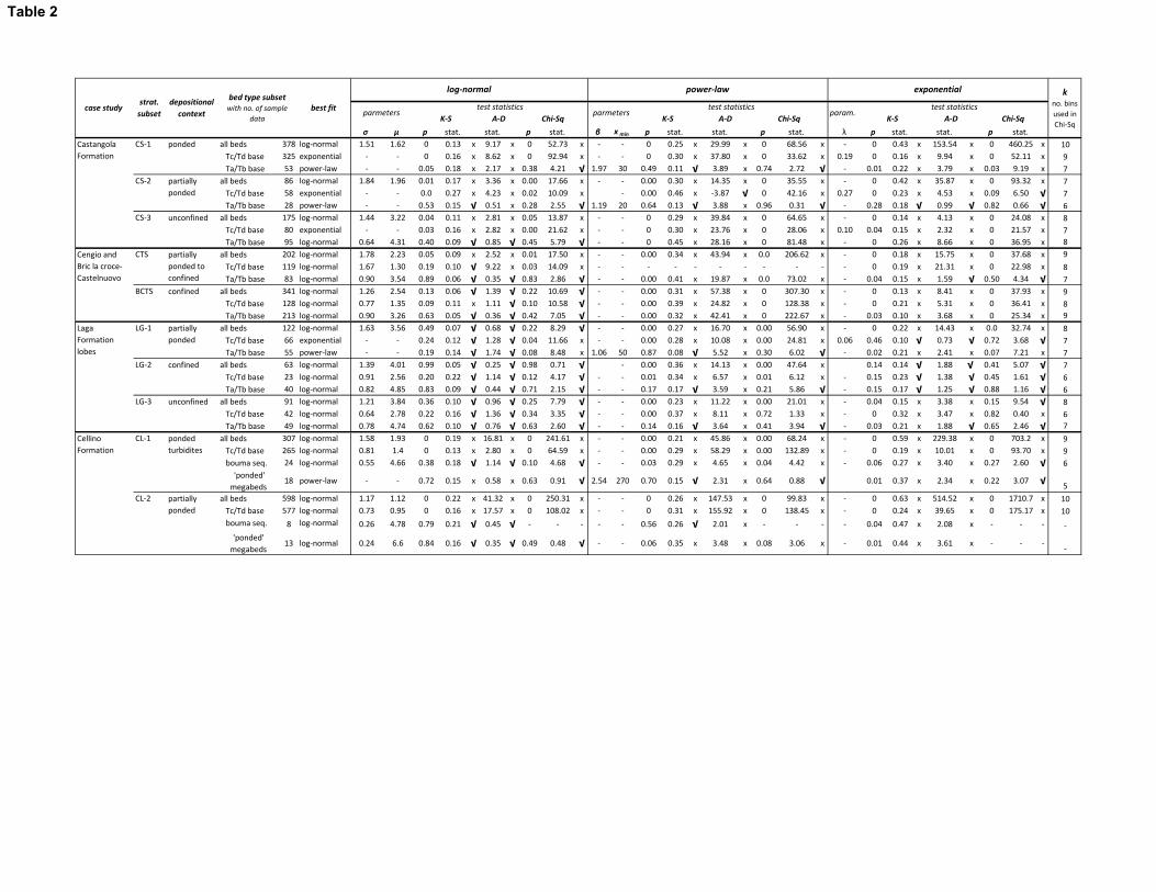
ʍ ʅ p stat. stat. p stat. ɴ x min p stat. stat. p stat. ʄ p stat. stat. p stat.

all beds 378 log-normal 1.51 1.62 0 0.13 x 9.17 x 0 52.73 x - - 0 0.25 x 29.99 x 0 68.56 x - 0 0.43 x 153.54 x 0 460.25 x 10

Tc/Td base 325 exponential - - 0 0.16 x 8.62 x 0 92.94 x - - 0 0.30 x 37.80 x 0 33.62 x 0.19 0 0.16 x 9.94 x 0 52.11 x 9

Ta/Tb base 53 power-law - - 0.05 0.18 x 2.17 x 0.38 4.21 к 1.97 30 0.49 0.11 к 3.89 x 0.74 2.72 к - 0.01 0.22 x 3.79 x 0.03 9.19 x 7

all beds 86 log-normal 1.84 1.96 0.01 0.17 x 3.36 x 0.00 17.66 x - - 0.00 0.30 x 14.35 x 0 35.55 x - 0 0.42 x 35.87 x 0 93.32 x 7

Tc/Td base 58 exponential - - 0.0 0.27 x 4.23 x 0.02 10.09 x - 0.00 0.46 x -3.87 к 0 42.16 x 0.27 0 0.23 x 4.53 x 0.09 6.50 к 7

Ta/Tb base 28 power-law - - 0.53 0.15 к 0.51 x 0.28 2.55 к 1.19 20 0.64 0.13 к 3.88 x 0.96 0.31 к - 0.28 0.18 к 0.99 к 0.82 0.66 к 6

all beds 175 log-normal 1.44 3.22 0.04 0.11 x 2.81 x 0.05 13.87 x - - 0 0.29 x 39.84 x 0 64.65 x - 0 0.14 x 4.13 x 0 24.08 x 8

Tc/Td base 80 exponential - - 0.03 0.16 x 2.82 x 0.00 21.62 x - - 0 0.30 x 23.76 x 0 28.06 x 0.10 0.04 0.15 x 2.32 x 0 21.57 x 7

Ta/Tb base 95 log-normal 0.64 4.31 0.40 0.09 к 0.85 к 0.45 5.79 к - - 0 0.45 x 28.16 x 0 81.48 x - 0 0.26 x 8.66 x 0 36.95 x 8

all beds 202 log-normal 1.78 2.23 0.05 0.09 x 2.52 x 0.01 17.50 x - - 0.00 0.34 x 43.94 x 0.0 206.62 x - 0 0.18 x 15.75 x 0 37.68 x 9

Tc/Td base 119 log-normal 1.67 1.30 0.19 0.10 к 9.22 x 0.03 14.09 x - - - - - - - - - - - 0 0.19 x 21.31 x 0 22.98 x 8

Ta/Tb base 83 log-normal 0.90 3.54 0.89 0.06 к 0.35 к 0.83 2.86 к - - 0.00 0.41 x 19.87 x 0.0 73.02 x - 0.04 0.15 x 1.59 к 0.50 4.34 к 7

all beds 341 log-normal 1.26 2.54 0.13 0.06 к 1.39 к 0.22 10.69 к - - 0.00 0.31 x 57.38 x 0 307.30 x - 0 0.13 x 8.41 x 0 37.93 x 9

Tc/Td base 128 log-normal 0.77 1.35 0.09 0.11 x 1.11 к 0.10 10.58 к - - 0.00 0.39 x 24.82 x 0 128.38 x - 0 0.21 x 5.31 x 0 36.41 x 8

Ta/Tb base 213 log-normal 0.90 3.26 0.63 0.05 к 0.36 к 0.42 7.05 к - - 0.00 0.32 x 42.41 x 0 222.67 x - 0.03 0.10 x 3.68 x 0 25.34 x 9

all beds 122 log-normal 1.63 3.56 0.49 0.07 к 0.68 к 0.22 8.29 к - - 0.00 0.27 x 16.70 x 0.00 56.90 x - 0 0.22 x 14.43 x 0.0 32.74 x 8

Tc/Td base 66 exponential - - 0.24 0.12 к 1.28 к 0.04 11.66 x - - 0.00 0.28 x 10.08 x 0.00 24.81 x 0.06 0.46 0.10 к 0.73 к 0.72 3.68 к 7

Ta/Tb base 55 power-law - - 0.19 0.14 к 1.74 к 0.08 8.48 x 1.06 50 0.87 0.08 к 5.52 x 0.30 6.02 к - 0.02 0.21 x 2.41 x 0.07 7.21 x 7

all beds 63 log-normal 1.39 4.01 0.99 0.05 к 0.25 к 0.98 0.71 к - 0.00 0.36 x 14.13 x 0.00 47.64 x 0.14 0.14 к 1.88 к 0.41 5.07 к 7

Tc/Td base 23 log-normal 0.91 2.56 0.20 0.22 к 1.14 к 0.12 4.17 к - - 0.01 0.34 x 6.57 x 0.01 6.12 x - 0.15 0.23 к 1.38 к 0.45 1.61 к 6

Ta/Tb base 40 log-normal 0.82 4.85 0.83 0.09 к 0.44 к 0.71 2.15 к - - 0.17 0.17 к 3.59 x 0.21 5.86 к - 0.15 0.17 к 1.25 к 0.88 1.16 к 6

all beds 91 log-normal 1.21 3.84 0.36 0.10 к 0.96 к 0.25 7.79 к - - 0.00 0.23 x 11.22 x 0.00 21.01 x - 0.04 0.15 x 3.38 x 0.15 9.54 к 8

Tc/Td base 42 log-normal 0.64 2.78 0.22 0.16 к 1.36 к 0.34 3.35 к - - 0.00 0.37 x 8.11 x 0.72 1.33 x - 0 0.32 x 3.47 x 0.82 0.40 x 6

Ta/Tb base 49 log-normal 0.78 4.74 0.62 0.10 к 0.76 к 0.63 2.60 к - - 0.14 0.16 к 3.64 x 0.41 3.94 к - 0.03 0.21 x 1.88 к 0.65 2.46 к 7

all beds 307 log-normal 1.58 1.93 0 0.19 x 16.81 x 0 241.61 x - - 0.00 0.21 x 45.86 x 0.00 68.24 x - 0 0.59 x 229.38 x 0 703.2 x 9

Tc/Td base 265 log-normal 0.81 1.4 0 0.13 x 2.80 x 0 64.59 x - - 0.00 0.29 x 58.29 x 0.00 132.89 x - 0 0.19 x 10.01 x 0 93.70 x 9

bouma seq. 24 log-normal 0.55 4.66 0.38 0.18 к 1.14 к 0.10 4.68 к - - 0.03 0.29 x 4.65 x 0.04 4.42 x - 0.06 0.27 x 3.40 x 0.27 2.60 к 6

'ponded'

megabeds18 power-law - - 0.72 0.15 x 0.58 x 0.63 0.91 к 2.54 270 0.70 0.15 к 2.31 x 0.64 0.88 к 0.01 0.37 x 2.34 x 0.22 3.07 к

5

all beds 598 log-normal 1.17 1.12 0 0.22 x 41.32 x 0 250.31 x - - 0 0.26 x 147.53 x 0 99.83 x - 0 0.63 x 514.52 x 0 1710.7 x 10

Tc/Td base 577 log-normal 0.73 0.95 0 0.16 x 17.57 x 0 108.02 x - - 0 0.31 x 155.92 x 0 138.45 x - 0 0.24 x 39.65 x 0 175.17 x 10

bouma seq. 8 log-normal 0.26 4.78 0.79 0.21 к 0.45 к - - - - - 0.56 0.26 к 2.01 x - - - - 0.04 0.47 x 2.08 x - - - -

'ponded'

megabeds13 log-normal 0.24 6.6 0.84 0.16 к 0.35 к 0.49 0.48 к - - 0.06 0.35 x 3.48 x 0.08 3.06 x - 0.01 0.44 x 3.61 x - - -

-

LG-3 unconfined

Cellino

Formation

CL-1 ponded

turbidites

CL-2 partially

ponded

Laga

Formation

lobes

LG-1 partially

ponded

LG-2 confined

Cengio and

Bric la croce-

Castelnuovo

CTS partially

ponded to

confined

BCTS confined

A-D Chi-Sq K-S A-D

Castangola

Formation

CS-1 ponded

CS-2 partially

ponded

CS-3 unconfined

K-S

log-normal

A-D Chi-Sq K-S

k no. bins

used in

Chi-Sq

case studystrat.

subset

depositional

context

bed type subset

with no. of sample

data

best fit

Chi-Sq

power-law exponential

parmeterstest statistics

parmeterstest statistics

param.test statistics

Table 2

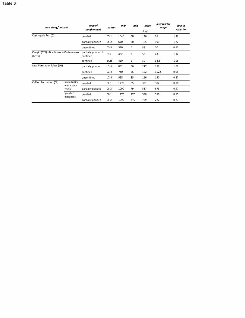
max min meaninterquartile

range

ponded CS-1 1040 30 140 95 1.41

partially ponded CS-2 670 20 105 109 1.22

unconfined CS-3 320 5 89 70 0.57

partially ponded to

confinedCTS 432 2 52 43 1.12

confined BCTS 410 2 39 32.5 1.08

partially ponded LG-1 892 50 217 199 1.02

confined LG-2 740 35 182 152.5 0.95

unconfined LG-3 595 35 156 140 0.87

ponded CL-1 1270 35 321 302 0.98

partially ponded CL-2 1090 79 517 675 0.67

ponded CL-1 1270 270 588 550 0.55

partially ponded CL-2 1090 440 759 222 0.23

Cengio (CTS) - Bric la croce-Castelnuovo

(BCTS)

Laga Formation lobes (LG)

Cellino Formation (CL) beds starting

with a basal

Ta/Tb

'ponded'

megabeds

Castangola Fm. (CS)

case study/datasettype of

confinementsubset

coef of

variation(cm)

Table 3