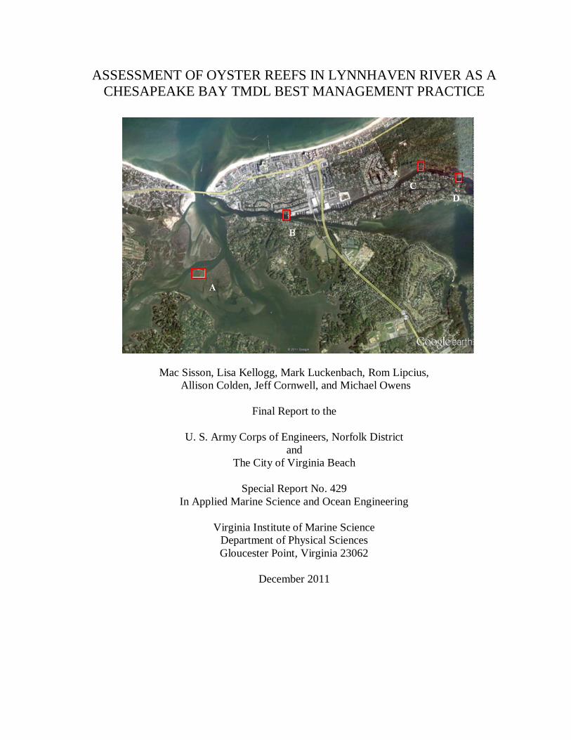
ASSESSMENT OF OYSTER REEFS IN LYNNHAVEN RIVER AS A

CHESAPEAKE BAY TMDL BEST MANAGEMENT PRACTICE

Mac Sisson, Lisa Kellogg, Mark Luckenbach, Rom Lipcius,

Allison Colden, Jeff Cornwell, and Michael Owens

Final Report to the

U. S. Army Corps of Engineers, Norfolk District

and

The City of Virginia Beach

Special Report No. 429

In Applied Marine Science and Ocean Engineering

Virginia Institute of Marine Science

Department of Physical Sciences

Gloucester Point, Virginia 23062

December 2011

i

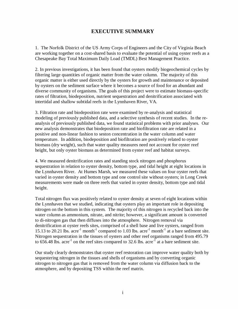
EXECUTIVE SUMMARY

1. The Norfolk District of the US Army Corps of Engineers and the City of Virginia Beach

are working together on a cost-shared basis to evaluate the potential of using oyster reefs as a

Chesapeake Bay Total Maximum Daily Load (TMDL) Best Management Practice.

2. In previous investigations, it has been found that oysters modify biogeochemical cycles by

filtering large quantities of organic matter from the water column. The majority of this

organic matter is either used directly by the oysters for growth and maintenance or deposited

by oysters on the sediment surface where it becomes a source of food for an abundant and

diverse community of organisms. The goals of this project were to estimate biomass-specific

rates of filtration, biodeposition, nutrient sequestration and denitrification associated with

intertidal and shallow subtidal reefs in the Lynnhaven River, VA.

3. Filtration rate and biodeposition rate were examined by re-analysis and statistical

modeling of previously published data, and a selective synthesis of recent studies. In the re-

analysis of previously published data, we found statistical problems with prior analyses. Our

new analysis demonstrates that biodeposition rate and biofiltration rate are related in a

positive and non-linear fashion to seston concentration in the water column and water

temperature. In addition, biodeposition and biofiltration are positively related to oyster

biomass (dry weight), such that water quality measures need not account for oyster reef

height, but only oyster biomass as determined from oyster reef and habitat surveys.

4. We measured denitrification rates and standing stock nitrogen and phosphorus

sequestration in relation to oyster density, bottom type, and tidal height at eight locations in

the Lynnhaven River. At Humes Marsh, we measured these values on four oyster reefs that

varied in oyster density and bottom type and one control site without oysters; in Long Creek

measurements were made on three reefs that varied in oyster density, bottom type and tidal

height.

Total nitrogen flux was positively related to oyster density at seven of eight locations within

the Lynnhaven that we studied, indicating that oysters play an important role in depositing

nitrogen on the bottom in this system. The majority of this nitrogen is recycled back into the

water column as ammonium, nitrate, and nitrite; however, a significant amount is converted

to di-nitrogen gas that then diffuses into the atmosphere. Nitrogen removal via

denitrification at oyster reefs sites, comprised of a shell base and live oysters, ranged from

15.13 to 20.21 lbs. acre-1

month-1

compared to 1.03 lbs. acre-1

month-1

at a bare sediment site.

Nitrogen sequestration in the tissues of oysters and other reef organisms ranged from 495.79

to 656.48 lbs. acre-1

on the reef sites compared to 32.6 lbs. acre-1

at a bare sediment site.

Our study clearly demonstrates that oyster reef restoration can improve water quality both by

sequestering nitrogen in the tissues and shells of organisms and by converting organic

nitrogen to nitrogen gas that is removed from the water column via diffusion back to the

atmosphere, and by depositing TSS within the reef matrix.

ii

5. Over the period 2005-2008, VIMS completed the successful development of an integrated

numerical modeling framework for the Lynnhaven River system. This framework combines

a high-resolution 3D hydrodynamic model (UnTRIM) that provides the required transport for

a water quality model (CE-QUAL-ICM) that, in turn, provides intra-tidal predictions of 23

water quality state variables. The hydrodynamic model underwent an extensive calibration

for surface elevation, salinity, and temperature and the water quality model was calibrated for

dissolved oxygen, chl-a, various forms of nitrogen and phosphorus, and total suspended

solids. Enhancements to these models to incorporate oyster reef dynamics are underway.

6. With respect to phosphorus, this investigation showed that there was no significant

reduction from the water column due to the presence of oyster reefs in the Lynnhaven based

on measurements of soluble reactive phosphorus flux measured under light and dark

conditions.

7. Regarding the removal of sediment from the water column due to oyster reefs, the amount

removed is controlled in large part by hydrodynamic advection, oyster biomass, seston

concentration, and water temperature. Determinations of the amounts removed can be

achieved through integration of the listed equations or more precisely through numerical

modeling that integrates the equations with hydrodynamic models.

Findings or recommendations contained herein do not constitute Corps of Engineers

approval of any project(s) or eliminate the need to follow normal regulatory permitting

processes.

iii

ACKNOWLEDGEMENTS

P. G. Ross, A. J. Birch, E. Smith, S. Fate, A. Curry, and P. Hollyman provided invaluable

assistance in the field and with sample processing. We thank R. Bonniwell and S. Bonniwell

for modifications to the laboratory to accommodate these studies and for assistance in the

field. We are indebted to Carol Pollard and the staff of the VIMS Analytical Services Center

for the nutrient analysis of faunal tissue samples. We are grateful to Mr. John Meekins for

allowing us to conduct a portion of our research on his leased oyster ground in the Humes

Marsh area. This work was supported by the City of Virginia Beach and the Norfolk District

of the U.S. Army Corps of Engineers on a cost-sharing basis under the Corps’ Section 22

Funding Program.

iv

TABLE OF CONTENTS

EXECUTIVE SUMMARY ......................................................................................................... i

ACKNOWLEDGEMENTS ....................................................................................................... iii

TABLE OF CONTENTS ......................................................................................................... iv

LIST OF TABLES .................................................................................................................... vi

LIST OF FIGURES .................................................................................................................. vii

I. INTRODUCTION ................................................................................................................. 1

II. METHODS ............................................................................................................................ 6

II-1. Study sites .............................................................................................................. 6

II-2. Measurement of oyster reef biogeochemical fluxes ................................................ 8

II-3. Incubation chamber design ..................................................................................... 8

II-4. Nutrient flux measurements.................................................................................... 9

Field deployment and retrieval ............................................................................ 9

Sample incubations ............................................................................................12

Water sample analyses .......................................................................................13

Membrane inlet mass spectrometry ..............................................................14

Solute analyses ............................................................................................14

II-5. Nutrient sequestration ..........................................................................................14

Macrofaunal abundance and biomass ................................................................14

Macrofaunal nutrient content .............................................................................15

II-6. Biomass-specific oyster filtration and biodeposition rates .....................................15

II-7. Statistical analyses ...............................................................................................15

III. RESULTS .........................................................................................................................16

III-1. Oyster density and biomass ..................................................................................16

III-2. Macrofauna biomass ............................................................................................18

III-3. Nutrient sequestration in macrofauna ...................................................................20

III-4. Flux measurements ..............................................................................................23

Oxygen flux ........................................................................................................23

Ammonium nitrogen flux ....................................................................................26

NO2 and NO3 nitrogen flux ..................................................................................28

Di-nitrogen nitrogen flux ....................................................................................31

Total nitrogen flux ..............................................................................................33

Nitrification and denitrification efficiency ..........................................................34

Nitrogen flux stoichiometry ................................................................................36

Soluble reactive phosphorus flux ........................................................................36

III-5. Biomass-specific oyster filtration and biodeposition rates .....................................37

IV. SUMMARY AND CONCLUSIONS ..................................................................................46

v

V. LITERATURE CITED .........................................................................................................52

vi

LIST OF TABLES

Table II.1. Description of sample locations, including nominal and measured oyster densities ........... 8

Table II.2. Chamber dimensions ................................................................................................. 9

Table II.3. Synopsis of flux measurement approach ........................................................................11

Table III.1. Measured oyster density and biomass at each sample site ...............................................16

Table III.2. Macrofauna abundance (g m-2

) by taxa from each other .................................................18

Table III.3. Macrofauna biomass density (g m-2

) by taxa from each other ..........................................19

Table III.4. Nitrogen and phosphorus conversions as a percent of dry weight.....................................20

Table III.5. Nitrogen sequestration (g m-2

) by taxa from each site .....................................................21

Table III.6. Phosphorus sequestration (g m-2

) by taxa from each site .................................................22

Table IV.1. Summary estimates of nitrogen fluxes and sequestration by site ......................................49

vii

LIST OF FIGURES

Figure I.1. Major nitrogen pathways on an oyster reef ................................................................ 3

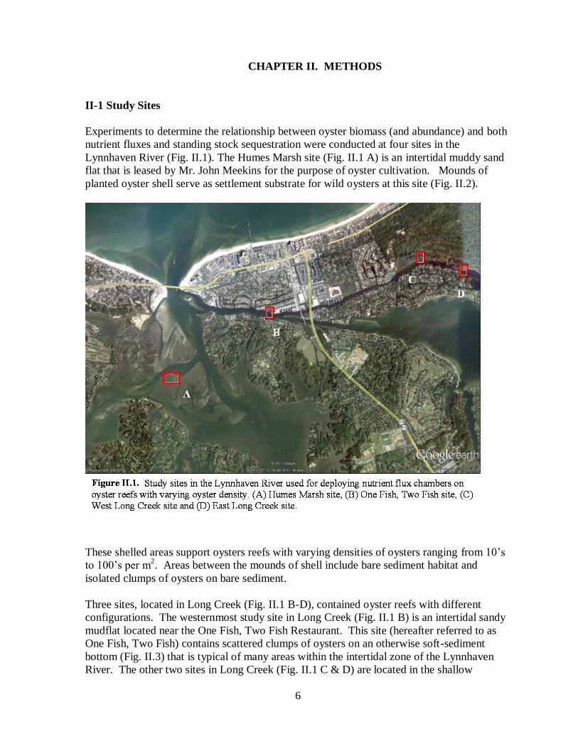
Figure II.1. Study sites in the Lynnhaven River used for deploying nutrient flux chambers on oyster

reefs with varying oyster density. (A) Humes Marsh site, (B) One Fish, Two Fish site, (C) West Long

Creek site and (D) East Long Creek site .......................................................................................... 6

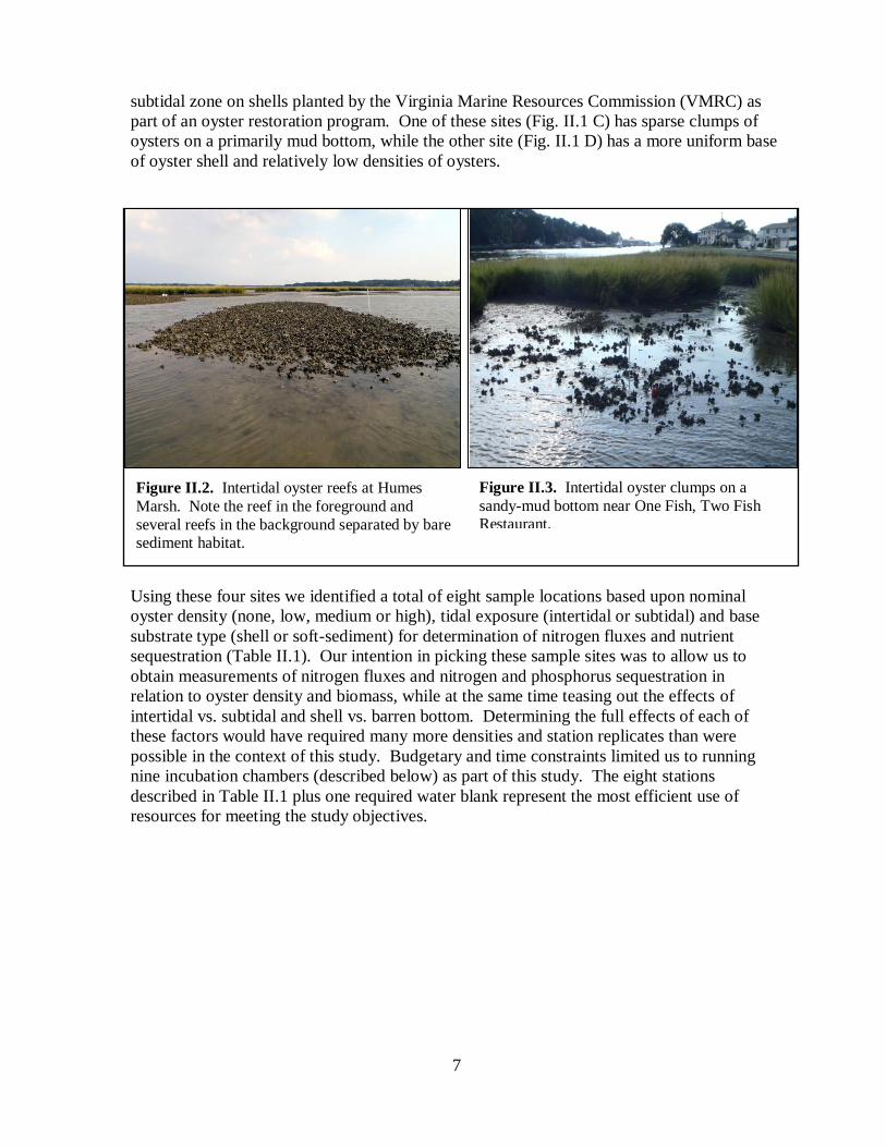
Figure II.2. Intertidal oyster reefs at Humes Marsh. Note the reef in the foreground and several reefs

in the background separated by bare sediment habitat ........................................................................ 7

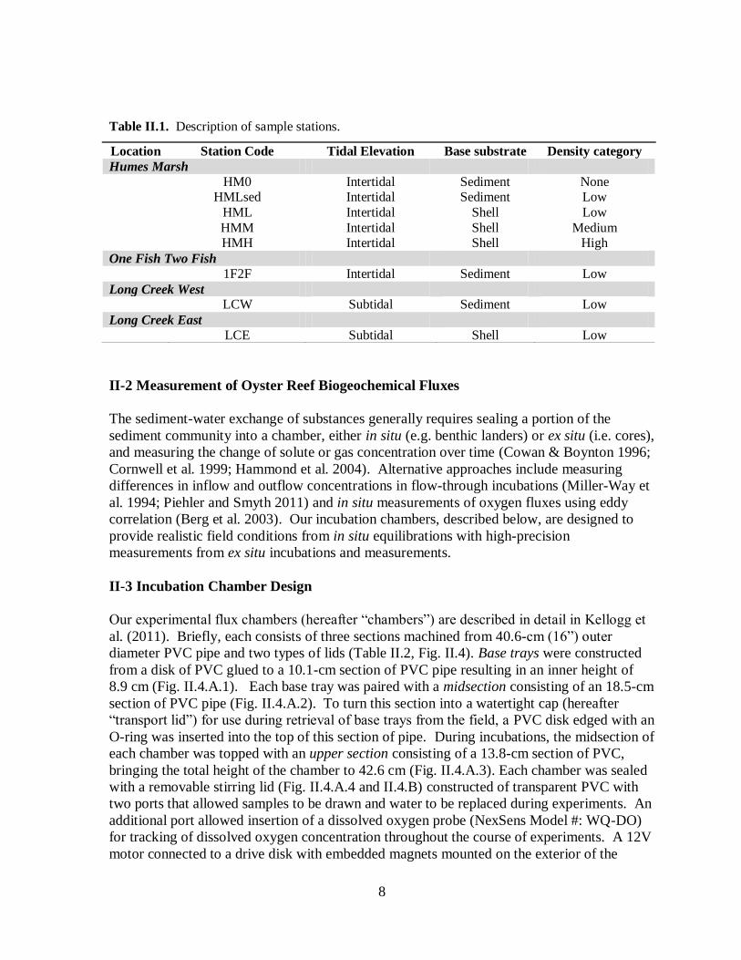
Figure II.3. Intertidal oyster clumps on a sandy-mud bottom near One Fish, Two Fish Restaurant ......... 7

Figure II.4. Photographs of an incubation chamber .........................................................................10

Figure II.5. Examples of chamber base trays embedded in the bottom at sample sites in the

Lynnhaven ..................................................................................................................................12

Figure II.6. Incubation chambers with stirring lids in place in the water bath ....................................13

Figure III.1. Size frequency distribution of oysters at (A) HMLsed, (B) HML, (C) HMM, (D) HMH,

(E) 1F2F, (F) LCW and (G) LCE...............................................................................................17

Figure III.2. Oxygen flux under light and dark conditions in incubation chambers from each

station .......................................................................................................................................23

Figure III.3. Oxygen flux under light and dark conditions in relation to soft tissue biomass of

macrobenthic organisms (including oysters) in the incubation chambers ....................................24

Figure III.4. Oxygen flux under light and dark conditions in relation to total biomass of

macrobenthic organisms in incubation chambers, inclusive of shells from live bivalves.............25

Figure III.5. Oxygen flux under light and dark conditions in relation to total biomass of

macrobenthic organisms in incubation chambers, inclusive of shells from live bivalves and

excluding the LCE site ..............................................................................................................25

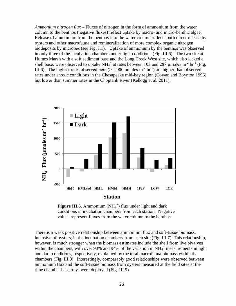
Figure III.6. Ammonium (NH4+) flux under light and dark conditions in incubation chambers

from each station .......................................................................................................................26

Figure III.7. Ammonium (NH4+) flux under light and dark conditions in relation to soft tissue

biomass of macrobenthic organisms (including oysters) in the incubation chambers ..................27

Figure III.8. Ammonium (NH4+) flux under light and dark conditions in relation to total biomass

in incubation chambers, inclusive of shells from live bivalves ...................................................27

viii

Figure III.9. Ammonium (NH4+) flux under light and dark conditions in relation to soft tissue

biomass at the field collection sites ............................................................................................28

Figure III.10. NO2+3 flux under light and dark conditions in incubation chambers from each

station .......................................................................................................................................29

Figure III.11. Nitrite and nitrate (NO2+3) flux under light and dark conditions in relation to

soft-tissue biomass of macrobenthic organisms in incubation chambers .....................................30

Figure III.12. Nitrite and nitrate (NO2+3) flux under light and dark conditions in relation to

total biomass (including shells of live bivalves) in incubation chambers ....................................30

Figure III.13. N2 nitrogen flux under light and dark conditions in incubation chambers from

each station ...............................................................................................................................31

Figure III.14. N2 flux under light and dark conditions in relation to soft-tissue biomass of

macrobenthic organisms in incubation chambers .......................................................................32

Figure III.15. N2 flux under light and dark conditions in relation to total biomass (including

shells of live bivalves) within incubation chambers ...................................................................32

Figure III.16. N2 flux under light and dark conditions in relation to soft-tissue biomass at the

field collection site ....................................................................................................................33

Figure III.17. Total nitrogen flux under light conditions at each station by nitrogen species .......33

Figure III.18. Total nitrogen flux under dark conditions at each station by nitrogen species .......34

Figure III.19. Percentages of total inorganic nitrogen flux attributable to nitrification and

denitrification in incubation chambers from each station ...........................................................35

Figure III.20. Relationship between oxygen flux and total nitrogen flux under light and dark

conditions in the incubation chambers from each station............................................................36

Figure III.21. Soluble reactive phosphorus flux under light and dark conditions in incubation

chambers from each station .......................................................................................................37

Figure III.22. Relationship between oyster shell height and dry mass (Oyster Mass =

0.00001(SH2.4

)) as adapted from Burke (2010) ..........................................................................38

Figure III.23. Plot of residuals against the fitted values of the regression ...................................39

Figure III.24. Non-random residuals with their leverage scores (influence upon the regression

model) .......................................................................................................................................40

Figure III.25. Biodeposition rates as a function of Seston concentration ...................................41

ix

Figure III.26. Relationship between Biodeposition Rates and Water Temperature ...................42

Figure III.27. Mesh plot of the function relating biodeposition rate to seston concentration

and water temperature. ..............................................................................................................44

Figure III.28. Mesh plot of the function relating biodeposition rate to seston concentration

and water temperature. ..............................................................................................................45

Figure IV.1. Total nitrogen flux as a function of oyster soft-tissue biomass at each of the field

sites ...........................................................................................................................................47

1

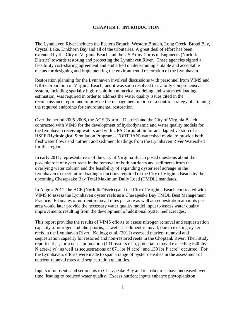
CHAPTER I. INTRODUCTION

The Lynnhaven River includes the Eastern Branch, Western Branch, Long Creek, Broad Bay,

Crystal Lake, Linkhorn Bay and all of the tributaries. A great deal of effort has been

extended by the City of Virginia Beach and the US Army Corps of Engineers (Norfolk

District) towards restoring and protecting the Lynnhaven River. These agencies signed a

feasibility cost-sharing agreement and embarked on determining suitable and acceptable

means for designing and implementing the environmental restoration of the Lynnhaven.

Restoration planning for the Lynnhaven involved discussions with personnel from VIMS and

URS Corporation of Virginia Beach, and it was soon resolved that a fully comprehensive

system, including spatially high-resolution numerical modeling and watershed loading

estimation, was required in order to address the water quality issues cited in the

reconnaissance report and to provide the management option of a control strategy of attaining

the required endpoints for environmental restoration.

Over the period 2005-2008, the ACE (Norfolk District) and the City of Virginia Beach

contracted with VIMS for the development of hydrodynamic and water quality models for

the Lynnhaven receiving waters and with URS Corporation for an adapted version of its

HSPF (Hydrological Simulation Program – FORTRAN) watershed model to provide both

freshwater flows and nutrient and sediment loadings from the Lynnhaven River Watershed

for this region.

In early 2011, representatives of the City of Virginia Beach posed questions about the

possible role of oyster reefs in the removal of both nutrients and sediments from the

overlying water column and the feasibility of expanding oyster reef acreage in the

Lynnhaven to meet future loading reductions required of the City of Virginia Beach by the

upcoming Chesapeake Bay Total Maximum Daily Load (TMDL) mandates.

In August 2011, the ACE (Norfolk District) and the City of Virginia Beach contracted with

VIMS to assess the Lynnhaven oyster reefs as a Chesapeake Bay TMDL Best Management

Practice. Estimates of nutrient removal rates per acre as well as sequestration amounts per

area would later provide the necessary water quality model input to assess water quality

improvements resulting from the development of additional oyster reef acreages.

This report provides the results of VIMS efforts to assess nitrogen removal and sequestration

capacity of nitrogen and phosphorus, as well as sediment removal, due to existing oyster

reefs in the Lynnhaven River. Kellogg et al. (2011) assessed nutrient removal and

sequestration capacity for restored and non-restored reefs in the Choptank River. Their study

reported that, for a dense population (131 oysters m-2

), potential removal exceeding 540 lbs

N acre-1 yr-1

as well as sequestrations of 871 lbs N acre-1

and 139 lbs P acre-1

occurred. For

the Lynnhaven, efforts were made to span a range of oyster densities in the assessment of

nutrient removal rates and sequestration quantities.

Inputs of nutrients and sediments to Chesapeake Bay and its tributaries have increased over

time, leading to reduced water quality. Excess nutrient inputs enhance phytoplankton

2

production and can lead to anoxic conditions in bottom waters. Excess sediment inputs can

lead to habitat degradation either by direct impacts (e.g. burial) or indirect impacts (e.g.

reduction of light reaching vegetated benthic habitats). In response to excess inputs, the U.S.

Environmental Protection Agency has imposed guidelines towards nutrient reduction goals

for point source discharges for nitrogen, phosphorus, and suspended sediments. As the

Lynnhaven has approximately 1050 outfalls draining its watershed into the receiving waters

of its three branches, the City of Virginia Beach is submitting its plan for nutrient and

sediment reduction to the Virginia Department of Conservation Resources (DCR).

The burden of meeting these reduction targets falls largely upon local governments, which

must look to a variety of options to reduce nutrient and sediment concentrations in the waters

adjacent to their jurisdictions. The City of Virginia Beach is faced with making significant

reductions in the nutrient and sediment concentrations in the Lynnhaven River. In addition

to meeting these goals by reducing the loadings of nitrogen, phosphorus, and sediments into

the Lynnhaven basin, the City is interested in evaluating the efficacy of using native oyster

restoration as a means to remove nutrients and sediment from the water column.

It has long been recognized that, through their filtration activity, oysters have the capacity to

affect water quality in Chesapeake Bay (Newell 1988) and other coastal waters (Dame et al.

1980). It is important to recognize, however, that filtration alone does not permanently

remove nutrients or sediment from the aquatic environment. Sediments may be resuspended

and nutrients undergo complex biogeochemical processes that ultimately determine their fate

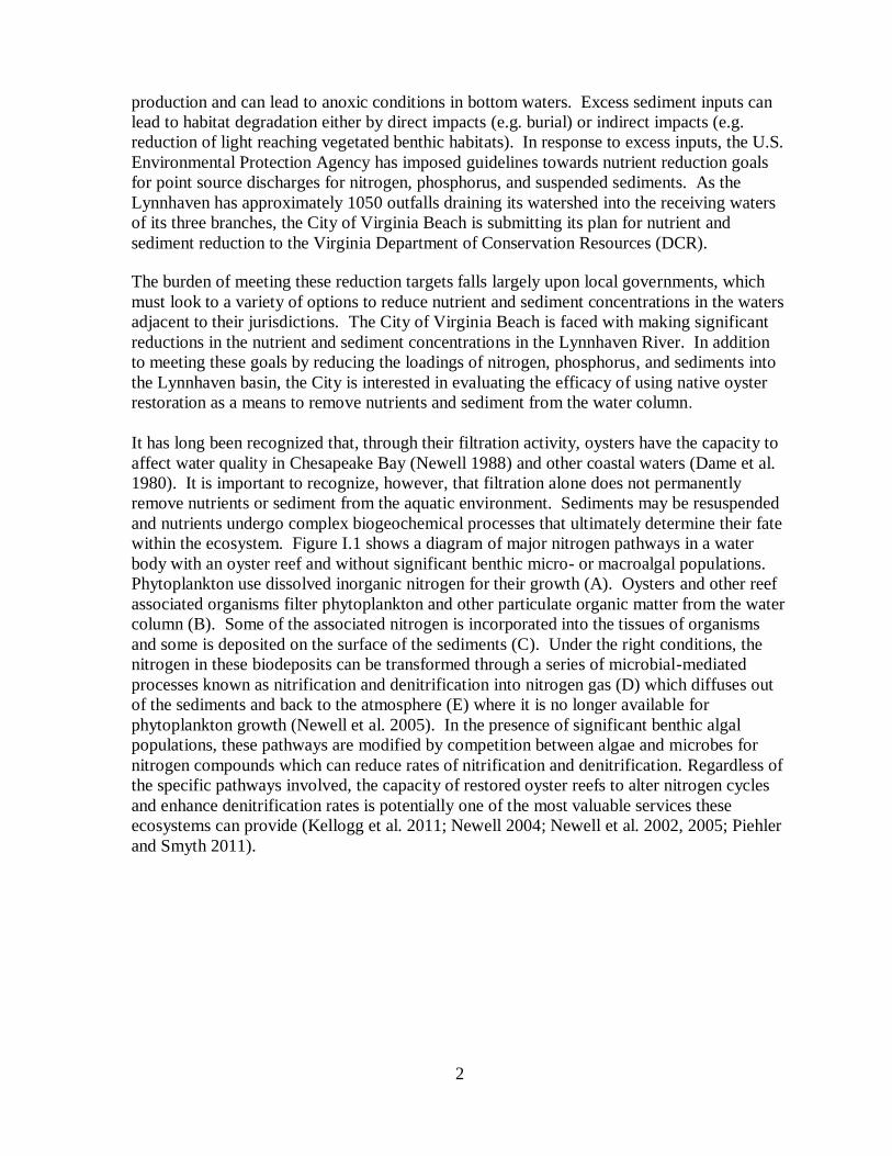
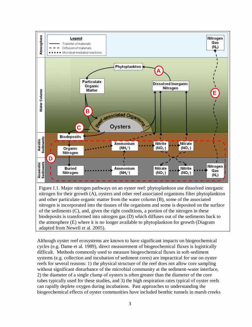
within the ecosystem. Figure I.1 shows a diagram of major nitrogen pathways in a water

body with an oyster reef and without significant benthic micro- or macroalgal populations.

Phytoplankton use dissolved inorganic nitrogen for their growth (A). Oysters and other reef

associated organisms filter phytoplankton and other particulate organic matter from the water

column (B). Some of the associated nitrogen is incorporated into the tissues of organisms

and some is deposited on the surface of the sediments (C). Under the right conditions, the

nitrogen in these biodeposits can be transformed through a series of microbial-mediated

processes known as nitrification and denitrification into nitrogen gas (D) which diffuses out

of the sediments and back to the atmosphere (E) where it is no longer available for

phytoplankton growth (Newell et al. 2005). In the presence of significant benthic algal

populations, these pathways are modified by competition between algae and microbes for

nitrogen compounds which can reduce rates of nitrification and denitrification. Regardless of

the specific pathways involved, the capacity of restored oyster reefs to alter nitrogen cycles

and enhance denitrification rates is potentially one of the most valuable services these

ecosystems can provide (Kellogg et al. 2011; Newell 2004; Newell et al. 2002, 2005; Piehler

and Smyth 2011).

3

A

C

B

D

E

Figure I.1. Major nitrogen pathways on an oyster reef: phytoplankton use dissolved inorganic

nitrogen for their growth (A), oysters and other reef associated organisms filter phytoplankton

and other particulate organic matter from the water column (B), some of the associated

nitrogen is incorporated into the tissues of the organisms and some is deposited on the surface

of the sediments (C), and, given the right conditions, a portion of the nitrogen in these

biodeposits is transformed into nitrogen gas (D) which diffuses out of the sediments back to

the atmosphere (E) where it is no longer available to phytoplankton for growth (Diagram

adapted from Newell et al. 2005).

Although oyster reef ecosystems are known to have significant impacts on biogeochemical

cycles (e.g. Dame et al. 1989), direct measurement of biogeochemical fluxes is logistically

difficult. Methods commonly used to measure biogeochemical fluxes in soft-sediment

systems (e.g. collection and incubation of sediment cores) are impractical for use on oyster

reefs for several reasons: 1) the physical structure of the reef does not allow core sampling

without significant disturbance of the microbial community at the sediment-water interface,

2) the diameter of a single clump of oysters is often greater than the diameter of the core

tubes typically used for these studies, and 3) the high respiration rates typical of oyster reefs

can rapidly deplete oxygen during incubations. Past approaches to understanding the

biogeochemical effects of oyster communities have included benthic tunnels in marsh creeks

4

(Dame et al. 1989), core incubations to simulate the effects of oyster biodeposits (Newell et

al. 2002; Holyoke 2008), and incubations of sediment cores collected adjacent to oyster

communities (Piehler and Smyth 2011). Recently, Kellogg et al. (2011) developed a

technique for directly measuring fluxes of di-nitrogen from oyster reefs that combines

inclusion of a realistic oyster reef benthic community with high precision measurements.

This technique was successfully employed to measure denitrification on a subtidal restored

oyster reef in Maryland.

Sequestration of nutrients in the tissues of reef organisms also represents a means of

removing nitrogen and phosphorus from the water column (Higgins et al. 2011; Kellogg et al.

2011). The extent to which this mechanism of nutrient removal assists in achieving TMDLs

will depend upon the length of time the nutrients are sequestered and/or the extent to which

they are transported out of the system. In general, nutrient sequestration in the tissues of

organisms only lasts as long as the soft tissues and hard structures they build as they grow

remain intact. Nutrients sequestered in the soft tissues of an oyster could remain sequestered

for years, whereas the nutrients sequestered in the tissues of an amphipod could last only a

few weeks if that amphipod dies without being consumed by another organism. Nutrients

sequestered in the calcium carbonate structures created by many organisms (e.g. the shells of

oysters) have the potential to sequester nutrients for years to decades (Powell et al. 2006)

and, if buried in sediments, centuries to millennia (Kirby et al. 1998). The fate of nutrients

sequestered in the tissues of reef organisms consumed by predators will depend upon a

variety of factors including the assimilation efficiency of the predator and its life history.

Oysters have the capacity through the deposition of feces and pseudofeces (collectively

called biodeposits; C in Fig. I.1) to remove large amounts of suspended sediments, as well as

organic matter, from the water column. Oyster reefs have been shown to enhance

sedimentation rates via accumulation of biodeposits (Haven and Morales-Alamo 1972) and

enhancement of sediment deposition (DeAlteris 1988). The topographically complex, three-

dimensional reef structures created by oysters as they grow alter flow characteristics in the

vicinity of the reef. The high density of roughness elements (i.e. oyster shells) creates both a

layer of decreased flow within the reef and increased turbulence in the overlying water

column. The increase in turbulence above the reef results in higher numbers of sediment

particles entering the reef matrix than would fall upon a soft sediment surface (i.e. mud or

sand). Once these particles enter the reef matrix, they encounter lower flow speeds that

result in greater rates of deposition. Once these particles have reached the surface of the

sediments within the reef matrix, resuspension rates are low because flow speeds and

turbulence at the sediment water interface are low. Another mechanism that enhances

sediment deposition and reduces resuspension on oyster reefs is feeding activities of oysters.

The seston that oysters filter from the water column contains suspended sediment particles in

addition to the phytoplankton and other organic particles that they ultimately consume. After

sorting sediment and other undesirable particles from the seston, these particles are packed in

mucus and deposited as pseudofeces. Because these particles are bound in mucus and now

have a larger effective particle size, they are less likely to be resuspended (Haven and

Morales-Alamo 1972).

To fully appreciate the role that oyster reefs can play in removing nutrients and sediments

from the water column we need to determine the size of the pools (i.e., the size of the boxes

5

in Fig. I.1) and the rate of fluxes between boxes (the magnitude of the arrows in Fig. I.1) and

we then need to incorporate these values into tributary-scale water quality models.

The 3D water quality model developed by VIMS for use in the Lynnhaven River is the US

Army Corps of Engineers model CE-QUAL-ICM. This model was initially developed as one

component of a model package employed to study eutrophication processes in Chesapeake

Bay (US Army ERDC 2000). ICM stands for "integrated compartment model," which is

analogous to the finite volume numerical method. The model computes and reports

concentrations, mass transport, kinetics transformations, and mass balances. This

eutrophication model computes 22 state variables including multiple forms of algae, carbon,

nitrogen, phosphorus, and silica, and dissolved oxygen. One significant feature of ICM is a

diagenetic sediment sub-model, which interactively predicts sediment-water oxygen and

nutrient fluxes. Alternatively, these fluxes may be specified based on observations.

The foundation of CE-QUAL-ICM is the solution to the three-dimensional mass-

conservation equation for a control volume based on the finite volume approach. Transport

within the CE-QUAL-ICM (Cerco and Cole 1995) is based on the integrated compartment

method (or box model methodology). The present version of CE-QUAL-ICM transport is a

loose extension of the original WASP code (Ambrose et al. 1986). The notion of utilizing the

box model concept was retained in order to allow the coupling, via map files, of ICM with

various hydrodynamic models. ICM represents "integrated compartment model," which is the

finite volume numerical method. The model computes constituent concentrations resulting

from transport and transformations in well-mixed cells that can be arranged in arbitrary

triangular and quadrilateral configurations.

Water quality data including dissolved oxygen, chlorophyll-a, TKN, ammonium, nitrate-

nitrite, and total phosphorus were collected by the Virginia Department of Environmental

Quality (VA-DEQ) at its 16 Lynnhaven stations over the 3-year period 2004-2006. The

successful calibration and validation of the CE-QUAL-ICM model for the Lynnhaven River

is confirmed by the quality of comparisons of model predictions to these data, as reported by

Sisson et al. (2010b), available online at: http://www.vims.edu/greylit/vims/sramsoe408.pdf

The goal of this study was to obtain critical data necessary for incorporating the effects of

oyster reefs on nutrient and sediment dynamics into the CE-QUAL-ICM water quality model

for the Lynnhaven River. Our specific objectives were to estimate (1) oyster filtration rates,

(2) biodeposition rates, (3) nutrient flux rates between the sediment and water column, and

(4) nutrient sequestration in relation to oyster biomass on reefs in the Lynnhaven River, with

the intent that these would then be used in subsequent work to incorporate these effects into

the water quality model to predict system-wide effects of oysters on water quality.

6

CHAPTER II. METHODS

II-1 Study Sites

Experiments to determine the relationship between oyster biomass (and abundance) and both

nutrient fluxes and standing stock sequestration were conducted at four sites in the

Lynnhaven River (Fig. II.1). The Humes Marsh site (Fig. II.1 A) is an intertidal muddy sand

flat that is leased by Mr. John Meekins for the purpose of oyster cultivation. Mounds of

planted oyster shell serve as settlement substrate for wild oysters at this site (Fig. II.2).

These shelled areas support oysters reefs with varying densities of oysters ranging from 10’s

to 100’s per m2. Areas between the mounds of shell include bare sediment habitat and

isolated clumps of oysters on bare sediment.

Three sites, located in Long Creek (Fig. II.1 B-D), contained oyster reefs with different

configurations. The westernmost study site in Long Creek (Fig. II.1 B) is an intertidal sandy

mudflat located near the One Fish, Two Fish Restaurant. This site (hereafter referred to as

One Fish, Two Fish) contains scattered clumps of oysters on an otherwise soft-sediment

bottom (Fig. II.3) that is typical of many areas within the intertidal zone of the Lynnhaven

River. The other two sites in Long Creek (Fig. II.1 C & D) are located in the shallow

7

subtidal zone on shells planted by the Virginia Marine Resources Commission (VMRC) as

part of an oyster restoration program. One of these sites (Fig. II.1 C) has sparse clumps of

oysters on a primarily mud bottom, while the other site (Fig. II.1 D) has a more uniform base

of oyster shell and relatively low densities of oysters.

Using these four sites we identified a total of eight sample locations based upon nominal

oyster density (none, low, medium or high), tidal exposure (intertidal or subtidal) and base

substrate type (shell or soft-sediment) for determination of nitrogen fluxes and nutrient

sequestration (Table II.1). Our intention in picking these sample sites was to allow us to

obtain measurements of nitrogen fluxes and nitrogen and phosphorus sequestration in

relation to oyster density and biomass, while at the same time teasing out the effects of

intertidal vs. subtidal and shell vs. barren bottom. Determining the full effects of each of

these factors would have required many more densities and station replicates than were

possible in the context of this study. Budgetary and time constraints limited us to running

nine incubation chambers (described below) as part of this study. The eight stations

described in Table II.1 plus one required water blank represent the most efficient use of

resources for meeting the study objectives.

Figure II.3. Intertidal oyster clumps on a

sandy-mud bottom near One Fish, Two Fish Restaurant.

Figure II.2. Intertidal oyster reefs at Humes

Marsh. Note the reef in the foreground and

several reefs in the background separated by bare sediment habitat.

8

II-2 Measurement of Oyster Reef Biogeochemical Fluxes

The sediment-water exchange of substances generally requires sealing a portion of the

sediment community into a chamber, either in situ (e.g. benthic landers) or ex situ (i.e. cores),

and measuring the change of solute or gas concentration over time (Cowan & Boynton 1996;

Cornwell et al. 1999; Hammond et al. 2004). Alternative approaches include measuring

differences in inflow and outflow concentrations in flow-through incubations (Miller-Way et

al. 1994; Piehler and Smyth 2011) and in situ measurements of oxygen fluxes using eddy

correlation (Berg et al. 2003). Our incubation chambers, described below, are designed to

provide realistic field conditions from in situ equilibrations with high-precision

measurements from ex situ incubations and measurements.

II-3 Incubation Chamber Design

Our experimental flux chambers (hereafter “chambers”) are described in detail in Kellogg et

al. (2011). Briefly, each consists of three sections machined from 40.6-cm (16”) outer

diameter PVC pipe and two types of lids (Table II.2, Fig. II.4). Base trays were constructed

from a disk of PVC glued to a 10.1-cm section of PVC pipe resulting in an inner height of

8.9 cm (Fig. II.4.A.1). Each base tray was paired with a midsection consisting of an 18.5-cm

section of PVC pipe (Fig. II.4.A.2). To turn this section into a watertight cap (hereafter

“transport lid”) for use during retrieval of base trays from the field, a PVC disk edged with an

O-ring was inserted into the top of this section of pipe. During incubations, the midsection of

each chamber was topped with an upper section consisting of a 13.8-cm section of PVC,

bringing the total height of the chamber to 42.6 cm (Fig. II.4.A.3). Each chamber was sealed

with a removable stirring lid (Fig. II.4.A.4 and II.4.B) constructed of transparent PVC with

two ports that allowed samples to be drawn and water to be replaced during experiments. An

additional port allowed insertion of a dissolved oxygen probe (NexSens Model #: WQ-DO)

for tracking of dissolved oxygen concentration throughout the course of experiments. A 12V

motor connected to a drive disk with embedded magnets mounted on the exterior of the

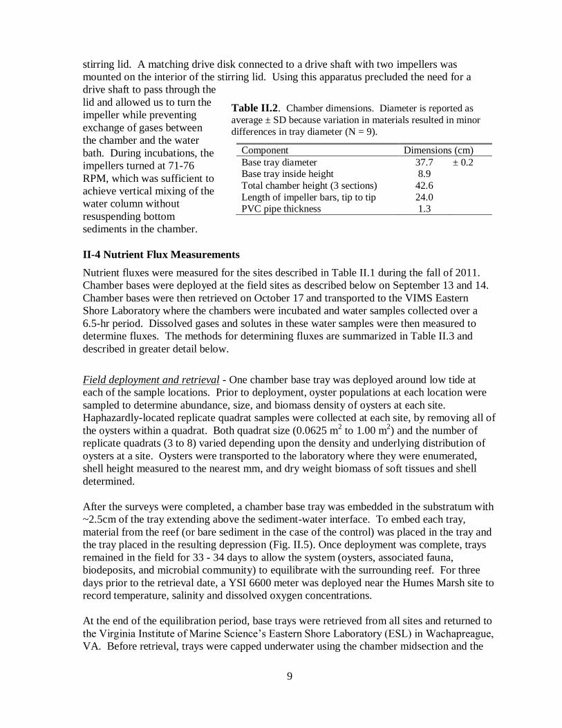
Table II.1. Description of sample stations.

Location Station Code Tidal Elevation Base substrate Density category

Humes Marsh

HM0 Intertidal Sediment None

HMLsed Intertidal Sediment Low

HML Intertidal Shell Low

HMM Intertidal Shell Medium

HMH Intertidal Shell High

One Fish Two Fish

1F2F Intertidal Sediment Low

Long Creek West

LCW Subtidal Sediment Low

Long Creek East

LCE Subtidal Shell Low

9

stirring lid. A matching drive disk connected to a drive shaft with two impellers was

mounted on the interior of the stirring lid. Using this apparatus precluded the need for a

drive shaft to pass through the

lid and allowed us to turn the

impeller while preventing

exchange of gases between

the chamber and the water

bath. During incubations, the

impellers turned at 71-76

RPM, which was sufficient to

achieve vertical mixing of the

water column without

resuspending bottom

sediments in the chamber.

II-4 Nutrient Flux Measurements

Nutrient fluxes were measured for the sites described in Table II.1 during the fall of 2011.

Chamber bases were deployed at the field sites as described below on September 13 and 14.

Chamber bases were then retrieved on October 17 and transported to the VIMS Eastern

Shore Laboratory where the chambers were incubated and water samples collected over a

6.5-hr period. Dissolved gases and solutes in these water samples were then measured to

determine fluxes. The methods for determining fluxes are summarized in Table II.3 and

described in greater detail below.

Field deployment and retrieval - One chamber base tray was deployed around low tide at

each of the sample locations. Prior to deployment, oyster populations at each location were

sampled to determine abundance, size, and biomass density of oysters at each site.

Haphazardly-located replicate quadrat samples were collected at each site, by removing all of

the oysters within a quadrat. Both quadrat size (0.0625 m2 to 1.00 m

2) and the number of

replicate quadrats (3 to 8) varied depending upon the density and underlying distribution of

oysters at a site. Oysters were transported to the laboratory where they were enumerated,

shell height measured to the nearest mm, and dry weight biomass of soft tissues and shell

determined.

After the surveys were completed, a chamber base tray was embedded in the substratum with

~2.5cm of the tray extending above the sediment-water interface. To embed each tray,

material from the reef (or bare sediment in the case of the control) was placed in the tray and

the tray placed in the resulting depression (Fig. II.5). Once deployment was complete, trays

remained in the field for 33 - 34 days to allow the system (oysters, associated fauna,

biodeposits, and microbial community) to equilibrate with the surrounding reef. For three

days prior to the retrieval date, a YSI 6600 meter was deployed near the Humes Marsh site to

record temperature, salinity and dissolved oxygen concentrations.

At the end of the equilibration period, base trays were retrieved from all sites and returned to

the Virginia Institute of Marine Science’s Eastern Shore Laboratory (ESL) in Wachapreague,

VA. Before retrieval, trays were capped underwater using the chamber midsection and the

Table II.2. Chamber dimensions. Diameter is reported as

average ± SD because variation in materials resulted in minor

differences in tray diameter (N = 9).

Component Dimensions (cm)

Base tray diameter 37.7 ± 0.2 Base tray inside height 8.9

Total chamber height (3 sections) 42.6

Length of impeller bars, tip to tip 24.0 PVC pipe thickness 1.3

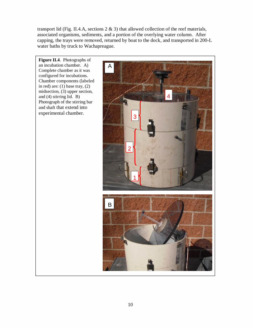
10

Figure II.4. Photographs of

an incubation chamber. A) Complete chamber as it was

configured for incubations.

Chamber components (labeled

in red) are: (1) base tray, (2) midsection, (3) upper section,

and (4) stirring lid. B)

Photograph of the stirring bar

and shaft that extend into

experimental chamber.

A

3

2

1

4

B.

transport lid (Fig. II.4.A, sections 2 & 3) that allowed collection of the reef materials,

associated organisms, sediments, and a portion of the overlying water column. After

capping, the trays were removed, returned by boat to the dock, and transported in 200-L

water baths by truck to Wachapreague.

11

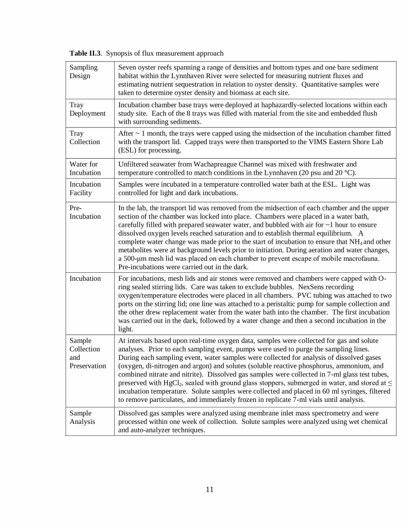
Table II.3. Synopsis of flux measurement approach

Sampling

Design

Seven oyster reefs spanning a range of densities and bottom types and one bare sediment

habitat within the Lynnhaven River were selected for measuring nutrient fluxes and

estimating nutrient sequestration in relation to oyster density. Quantitative samples were taken to determine oyster density and biomass at each site.

Tray

Deployment

Incubation chamber base trays were deployed at haphazardly-selected locations within each

study site. Each of the 8 trays was filled with material from the site and embedded flush with surrounding sediments.

Tray

Collection

After ~ 1 month, the trays were capped using the midsection of the incubation chamber fitted

with the transport lid. Capped trays were then transported to the VIMS Eastern Shore Lab (ESL) for processing.

Water for

Incubation

Unfiltered seawater from Wachapreague Channel was mixed with freshwater and

temperature controlled to match conditions in the Lynnhaven (20 psu and 20 °C).

Incubation

Facility

Samples were incubated in a temperature controlled water bath at the ESL. Light was

controlled for light and dark incubations.

Pre-

Incubation

In the lab, the transport lid was removed from the midsection of each chamber and the upper

section of the chamber was locked into place. Chambers were placed in a water bath, carefully filled with prepared seawater water, and bubbled with air for ~1 hour to ensure

dissolved oxygen levels reached saturation and to establish thermal equilibrium. A

complete water change was made prior to the start of incubation to ensure that NH4 and other metabolites were at background levels prior to initiation. During aeration and water changes,

a 500-μm mesh lid was placed on each chamber to prevent escape of mobile macrofauna.

Pre-incubations were carried out in the dark.

Incubation For incubations, mesh lids and air stones were removed and chambers were capped with O-

ring sealed stirring lids. Care was taken to exclude bubbles. NexSens recording

oxygen/temperature electrodes were placed in all chambers. PVC tubing was attached to two

ports on the stirring lid; one line was attached to a peristaltic pump for sample collection and the other drew replacement water from the water bath into the chamber. The first incubation

was carried out in the dark, followed by a water change and then a second incubation in the

light.

Sample

Collection

and Preservation

At intervals based upon real-time oxygen data, samples were collected for gas and solute

analyses. Prior to each sampling event, pumps were used to purge the sampling lines.

During each sampling event, water samples were collected for analysis of dissolved gases (oxygen, di-nitrogen and argon) and solutes (soluble reactive phosphorus, ammonium, and

combined nitrate and nitrite). Dissolved gas samples were collected in 7-ml glass test tubes,

preserved with HgCl2, sealed with ground glass stoppers, submerged in water, and stored at ≤

incubation temperature. Solute samples were collected and placed in 60 ml syringes, filtered to remove particulates, and immediately frozen in replicate 7-ml vials until analysis.

Sample

Analysis

Dissolved gas samples were analyzed using membrane inlet mass spectrometry and were

processed within one week of collection. Solute samples were analyzed using wet chemical and auto-analyzer techniques.

12

Sample incubations – All chambers were delivered to the VIMS-ESL within three hours of

collection from the field. More than 24 hours prior to the expected arrival of the chambers,

holding tanks in the laboratory were filled with a mixture of unfiltered seawater from

Wachapreague Channel and freshwater to match the salinity at the Lynnhaven River sites.

Seawater temperature in the holding tanks was maintained at the measured temperature at the

time of retrieval in the Lynnhaven. Upon arrival at the ESL, the transport lid was removed

from the midsection of each chamber and the upper section of the chamber was locked into

place (Fig. II.4.A.3). Chambers were then placed in the water bath, carefully filled with

prepared water, and bubbled with air for >1 hour to bring dissolved oxygen levels to

saturation. During aeration, a 500-μm mesh lid was placed on each chamber to prevent

escape of mobile macrofauna. An empty chamber was also placed in the water bath and

served as a seawater control (hereafter “blank”), bringing the total number of chambers

sampled during each set of experiments to nine. Prior to the start of the incubations, water in

the baths was drained and replaced with water from the holding tanks to ensure that levels of

ammonia and other compounds were similar to background levels at the start of incubations.

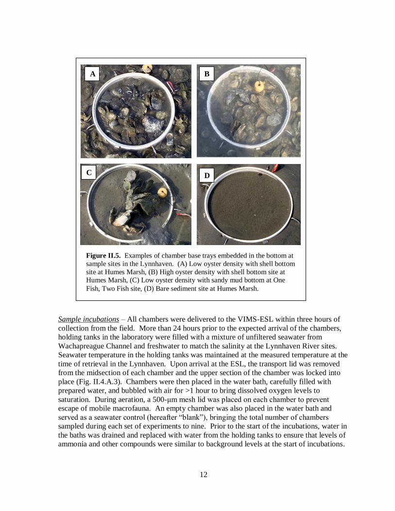
Figure II.5. Examples of chamber base trays embedded in the bottom at

sample sites in the Lynnhaven. (A) Low oyster density with shell bottom

site at Humes Marsh, (B) High oyster density with shell bottom site at Humes Marsh, (C) Low oyster density with sandy mud bottom at One

Fish, Two Fish site, (D) Bare sediment site at Humes Marsh.

A B

D C

13

Incubations were conducted under both light and dark conditions. Dark incubations began

within 5 hours of collection of the first sample in the field and were followed by incubations

under light conditions. Prior to starting the incubations, mesh lids and air stones were

removed from chambers and replaced with stirring lids. Because respiration rates were

expected to be highest in chambers containing the highest oyster biomass, the seawater blank

chamber and the chambers with lower oyster biomass were sealed with stirring lids before

the chambers with higher oyster biomass. Each stirring lid was edged with an O-ring and

fitted with a sampling line, a water replacement line, and a dissolved oxygen probe. The

sampling line consisted of 3.2-mm inner diameter PVC tubing; one end was attached to a

port on the chamber lid and the other to a peristaltic pump. The water replacement line was

constructed of the same tubing and drew replacement water from the water bath in which the

chamber was immersed. An oxygen electrode (NexSens Model #: WQ-DO) was inserted

into each chamber lid through an O-ring sealed port (Fig. II.6). During sealing of chambers

with stirring lids, care was taken to ensure that no gas bubbles were trapped in the chamber.

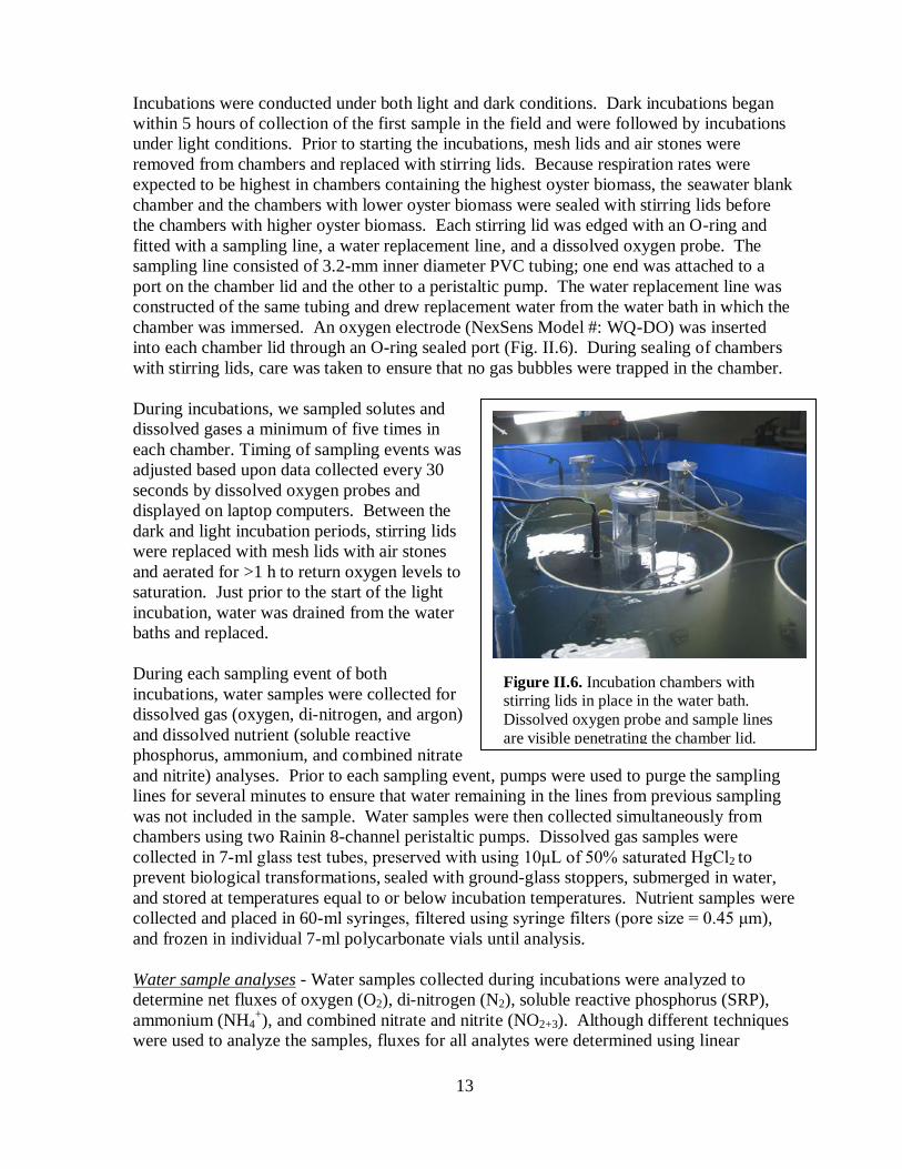
During incubations, we sampled solutes and

dissolved gases a minimum of five times in

each chamber. Timing of sampling events was

adjusted based upon data collected every 30

seconds by dissolved oxygen probes and

displayed on laptop computers. Between the

dark and light incubation periods, stirring lids

were replaced with mesh lids with air stones

and aerated for >1 h to return oxygen levels to

saturation. Just prior to the start of the light

incubation, water was drained from the water

baths and replaced.

During each sampling event of both

incubations, water samples were collected for

dissolved gas (oxygen, di-nitrogen, and argon)

and dissolved nutrient (soluble reactive

phosphorus, ammonium, and combined nitrate

and nitrite) analyses. Prior to each sampling event, pumps were used to purge the sampling

lines for several minutes to ensure that water remaining in the lines from previous sampling

was not included in the sample. Water samples were then collected simultaneously from

chambers using two Rainin 8-channel peristaltic pumps. Dissolved gas samples were

collected in 7-ml glass test tubes, preserved with using 10μL of 50% saturated HgCl2 to

prevent biological transformations, sealed with ground-glass stoppers, submerged in water,

and stored at temperatures equal to or below incubation temperatures. Nutrient samples were

collected and placed in 60-ml syringes, filtered using syringe filters (pore size = 0.45 μm),

and frozen in individual 7-ml polycarbonate vials until analysis.

Water sample analyses - Water samples collected during incubations were analyzed to

determine net fluxes of oxygen (O2), di-nitrogen (N2), soluble reactive phosphorus (SRP),

ammonium (NH4+), and combined nitrate and nitrite (NO2+3). Although different techniques

were used to analyze the samples, fluxes for all analytes were determined using linear

Figure II.6. Incubation chambers with stirring lids in place in the water bath.

Dissolved oxygen probe and sample lines

are visible penetrating the chamber lid.

14

regressions fitted to plots of concentration versus time. To remove the influence of water

column processes from our results, slopes of regression lines were adjusted using data from

the blank chamber when these data indicated a significant flux of an analyte. Fluxes were

considered significant when the regression line had an R-squared value ≥0.80 and the

difference between data in a time course was greater than the precision of the method used

for analysis.

Membrane inlet mass spectrometry - Membrane inlet mass spectrometry, a high-precision

rapid method for analyzing concentrations of dissolved gases (Kana et al. 1994), was used to

determine the concentrations of N2 and O2 in our samples. Briefly, each sample was

analyzed by bringing it to constant temperature, pumping it at a constant rate through a

silicone membrane in the vacuum inlet of a quadrupole mass spectrometer, monitoring the

signals from the mass spectrometer for N2, O2, and argon (Ar), constantly calculating gas

ratios (N2:Ar and O2:Ar) until they stabilized, and recording these stable values. In practice,

this technique yields coefficients of variation for gas ratios of ~0.02%. During the first

sampling event of the dark incubation, duplicate samples were collected and replicate

analyses were conducted and used as an internal precision check of the method.

Solute analysis - All dissolved nutrient analyses were carried out by the Analytical Services

laboratory at Horn Point Laboratory following standard procedures. Soluble reactive

phosphorus (SRP) was analyzed using a phosphomolybdate colorimetric analysis (Parsons et

al. 1984) with a detection limit of <0.005 mg L-1

. NH4+ concentrations were determined

using phenol/hypochlorite colorimetry (Parsons et al. 1984). Combined NO2+3

concentrations were determined using Cd reduction of NO3 to NO2 with a detection limit of

<0.03 mg L-1

(Parsons et al. 1984).

II-5 Nutrient sequestration

Once incubations were complete, stirring lids were removed and samples were again aerated

and capped with 500-μm mesh lids. Chambers were then held in the water bath until they

were processed to collect all macrofauna retained on a 1.0-mm sieve. While chambers

awaited processing, bath water was replaced as needed with salinity-adjusted, filtered

seawater from Wachapreague Channel.

Macrofaunal Abundance and Biomass - Macrofauna were collected by rinsing all of the

substrate in the incubation chambers through a 1.0-mm mesh sieve. Oyster shells were

carefully broken apart and rinsed in freshwater to remove polychaetes (primarily Allita

succinea) that are often found within interstitial space within the shell. Larger macrofauna

and macrofauna attached to large oysters shells were frozen for later analyses. All other

material retained on the sieves was fixed in 10% buffered formalin. After a minimum of 48

hours in formalin, samples were rinsed thoroughly and transferred to 70% ethanol. All

organisms in both frozen and preserved samples were then identified to the lowest practical

taxonomic level and enumerated. Dry weight biomass for whole organisms was then

determined by drying at 60 °C for a minimum of 48 hours and weighing to the nearest 0.1

mg. For oysters, ribbed mussels (Geukenisia demissa) and hard clams (Mercenaria

mercenaria), soft tissue was first removed from the shell and dry weights were determined

separately for shell and soft tissue for all but the smallest individuals.

15

Macrofaunal Nutrient Content - Nitrogen and phosphorus content for each major faunal

group in our samples were estimated by one of two methods. For those faunal groups

analyzed by Kellogg et al. (2011) previously determined values for N and P as percentages of

dry weight biomass were used. For other faunal groups, we haphazardly selected a minimum

of three individuals from each group and the VIMS Analytical Services Laboratory analyzed

nitrogen content using a CHN analyzer and phosphorus content using colorimetric analysis.

Nitrogen and phosphorus content were then reported as a percent of dry tissue weight and

total N and P sequestered by macrofauna in the sample determined by multiplication.

II-6 Biomass-specific oyster filtration and biodeposition rates

Biodeposition and biofiltration rates were analyzed from a database generated by Jordan

(1987). This is a unique data set that was never published in the peer-reviewed scientific

literature, and which was derived from a series of mesocosm studies that examined

biodeposition rates of the eastern oyster as a function of seston concentration, water

temperature, and salinity (Jordan 1987). We re-analyzed the data using non-linear regression

models. In addition, we evaluated the available literature on biodeposition and biofiltration

rates most relevant to the project goals.

II-7 Statistical analyses

Following square root transformation to meet the assumption of normality, we tested for

differences between abundance and biomass density of oysters at each of the study sites

using one-way ANOVAs. Pairwise multiple comparisons tests with an experiment-wise

error rate=0.05 were then used to identify significant differences in abundance and in

biomass between our eight sampling stations.

16

CHAPTER III. RESULTS

III-1 Oyster density and biomass

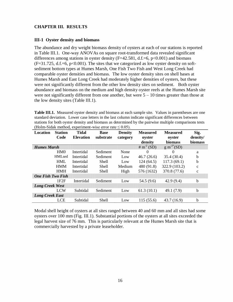
The abundance and dry weight biomass density of oysters at each of our stations is reported

in Table III.1. One-way ANOVAs on square root-transformed data revealed significant

differences among stations in oyster density (F=42.581, d.f.=6, p<0.001) and biomass

(F=31.725, d.f.=6, p<0.001). The sites that we categorized as low oyster density on soft-

sediment bottom types at Humes Marsh, One Fish Two Fish and West Long Creek had

comparable oyster densities and biomass. The low oyster density sites on shell bases at

Humes Marsh and East Long Creek had moderately higher densities of oysters, but these

were not significantly different from the other low density sites on sediment. Both oyster

abundance and biomass on the medium and high density oyster reefs at the Humes Marsh site

were not significantly different from one another, but were 5 – 10 times greater than those at

the low density sites (Table III.1).

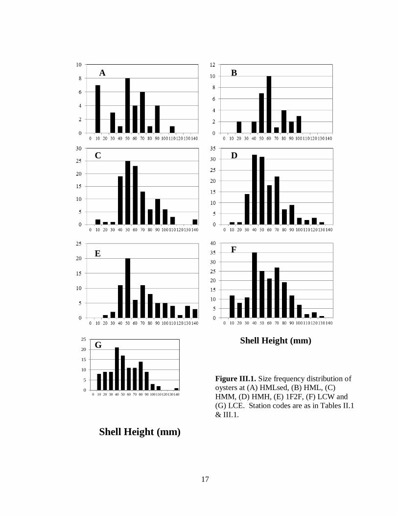
Modal shell height of oysters at all sites ranged between 40 and 60 mm and all sites had some

oysters over 100 mm (Fig. III.1). Substantial portions of the oysters at all sites exceeded the

legal harvest size of 76 mm. This is particularly relevant at the Humes Marsh site that is

commercially harvested by a private leaseholder.

Table III.1. Measured oyster density and biomass at each sample site. Values in parentheses are one

standard deviation. Lower case letters in the last column indicate significant differences between

stations for both oyster density and biomass as determined by the pairwise multiple comparisons tests

(Holm-Sidak method, experiment-wise error rate ≤ 0.05).

Location Station

Code

Tidal

Elevation

Base

substrate

Density

category

Measured

oyster

density

Measured

oyster

biomass

Sig.

density/

biomass

Humes Marsh # m-2 (SD) g m

-2*(SD)

HM0 Intertidal Sediment None 0 0 a

HMLsed Intertidal Sediment Low 46.7 (26.6) 35.4 (30.4) b

HML Intertidal Shell Low 124 (64.5) 117.3 (69.1) b

HMM Intertidal Shell Medium 480 (91.8) 322.9 (103.2) c

HMH Intertidal Shell High 576 (1632) 370.8 (77.6) c

One Fish Two Fish

1F2F Intertidal Sediment Low 54.5 (9.6) 42.9 (9.4) b

Long Creek West

LCW Subtidal Sediment Low 61.3 (10.1) 49.1 (7.9) b

Long Creek East

LCE Subtidal Shell Low 115 (55.6) 43.7 (16.9) b

17

Shell Height (mm)

A B

C D

E F

G

0

5

10

15

20

25

0 10 20 30 40 50 60 70 80 90 100110120130140

Figure III.1. Size frequency distribution of

oysters at (A) HMLsed, (B) HML, (C)

HMM, (D) HMH, (E) 1F2F, (F) LCW and

(G) LCE. Station codes are as in Tables II.1

& III.1.

Shell Height (mm)

18

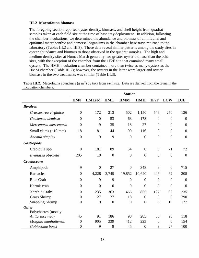
III-2 Macrofauna biomass

The foregoing section reported oyster density, biomass, and shell height from quadrat

samples taken at each field site at the time of base tray deployment. In addition, following

the chamber incubations, we determined the abundance and biomass of all infaunal and

epifaunal macrobenthic and demersal organisms in the chamber base trays returned to the

laboratory (Tables III.2 and III.3). These data reveal similar patterns among the study sites in

oyster abundance and biomass to those observed in the quadrat samples. The high and

medium density sites at Humes Marsh generally had greater oyster biomass than the other

sites, with the exception of the chamber from the 1F2F site that contained many small

oysters. The HMH incubation chamber contained more than twice as many oysters as the

HMM chamber (Table III.2); however, the oysters in the latter were larger and oyster

biomass in the two treatments was similar (Table III.3).

Table III.2. Macrofauna abundance (g m

-2) by taxa from each site. Data are derived from the fauna in the

incubation chambers.

Station

HM0 HMLsed HML HMM HMH 1F2F LCW LCE

Bivalves

Crassostrea virginica 0 172 213 502 1,150 546 250 136

Geukensia demissa 0 0 53 63 178 0 0 0

Mercenaria mercenaria 0 9 35 18 27 9 0 0

Small clams (<10 mm) 18 81 44 99 116 0 0 0

Anomia simplex 0 9 9 0 0 0 9 0

Gastropods

Crepidula spp. 0 181 89 54 0 0 71 72

Ilyanassa obsoleta 205 18 0 0 0 0 0 0

Crustaceans

Amphipods 9 0 27 0 348 9 0 715

Barnacles 0 4,228 3,749 19,852 10,640 446 62 208

Blue Crab 0 9 9 0 0 9 0 0

Hermit crab 0 0 0 9 0 0 0 0

Xanthid Crabs 0 235 363 466 855 127 62 235

Grass Shrimp 0 27 27 18 0 0 0 290

Snapping Shrimp 0 0 0 0 0 0 18 127

Other

Polychaetes (mostly

Alitta succinea) 45 91 186 90 285 55 98 118

Molgula manhattensis 0 905 239 412 223 0 0 154

Gobiosoma bosci 0 9 9 45 0 9 27 100

19

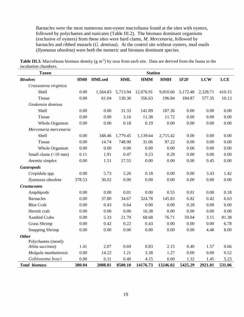
Barnacles were the most numerous non-oyster macrofauna found at the sites with oysters,

followed by polychaetes and tunicates (Table III.2). The biomass dominant organisms

(exclusive of oysters) from these sites were hard clams, M. Mercenaria, followed by

barnacles and ribbed mussels (G. demissa). At the control site without oysters, mud snails

(Ilyanassa obsoleta) were both the numeric and biomass dominant species.

Table III.3. Macrofauna biomass density (g m-2

) by taxa from each site. Data are derived from the fauna in the

incubation chambers.

Taxon Station

Bivalves HM0 HMLsed HML HMM HMH 1F2F LCW LCE

Crassostrea virginica

Shell 0.00 1,564.83 5,713.94 12,076.91 9,810.66 5,172.48 2,328.71 410.15

Tissue 0.00 61.04 130.30 356.63 196.84 184.87 577.35 10.13

Geukensia demissa

Shell 0.00 0.00 31.33 141.89 187.36 0.00 0.00 0.00

Tissue 0.00 0.00 3.16 11.38 11.72 0.00 0.00 0.00

Whole Organism 0.00 0.00 0.18 0.19 0.00 0.00 0.00 0.00

Mercenaria mercenaria

Shell 0.00 348.46 1,779.45 1,139.64 2,715.42 0.00 0.00 0.00

Tissue 0.00 14.74 748.90 31.06 97.22 0.00 0.00 0.00

Whole Organism 0.00 0.00 0.00 0.00 0.00 0.06 0.00 0.00

Small clams (<10 mm) 0.11 1.91 0.47 0.23 0.29 0.00 0.00 0.00

Anomia simplex 0.00 1.51 27.55 0.00 0.00 0.00 0.45 0.00

Gastropods

Crepidula spp. 0.00 5.73 5.26 0.18 0.00 0.00 3.43 1.42

Ilyanassa obsoleta 378.53 30.02 0.00 0.00 0.00 0.00 0.00 0.00

Crustaceans

Amphipods 0.00 0.00 0.01 0.00 0.55 0.01 0.00 0.18

Barnacles 0.00 37.80 34.67 324.78 145.83 6.82 0.42 6.63

Blue Crab 0.00 0.43 0.64 0.00 0.00 0.28 0.00 0.00

Hermit crab 0.00 0.00 0.00 16.38 0.00 0.00 0.00 0.00

Xanthid Crabs 0.00 5.33 21.70 68.68 76.71 59.04 3.15 81.38

Grass Shrimp 0.00 0.42 0.22 0.43 0.00 0.00 0.00 6.78

Snapping Shrimp 0.00 0.00 0.00 0.00 0.00 0.00 4.48 8.00

Other

Polychaetes (mostly

Alitta succinea) 1.41 2.07 0.69 0.83 2.15 0.40 1.57 0.66

Molgula manhattensis 0.00 14.22 1.21 3.38 1.27 0.00 0.00 0.52

Gobiosoma bosci 0.00 0.31 0.40 4.15 0.00 1.32 1.45 5.23

Total biomass 380.04 2088.81 8500.10 14176.73 13246.02 5425.29 2921.01 531.06

20

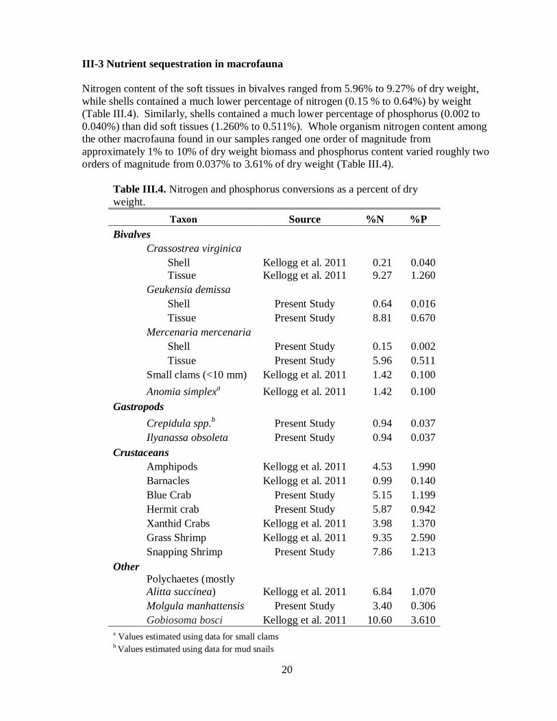
III-3 Nutrient sequestration in macrofauna

Nitrogen content of the soft tissues in bivalves ranged from 5.96% to 9.27% of dry weight,

while shells contained a much lower percentage of nitrogen (0.15 % to 0.64%) by weight

(Table III.4). Similarly, shells contained a much lower percentage of phosphorus (0.002 to

0.040%) than did soft tissues (1.260% to 0.511%). Whole organism nitrogen content among

the other macrofauna found in our samples ranged one order of magnitude from

approximately 1% to 10% of dry weight biomass and phosphorus content varied roughly two

orders of magnitude from 0.037% to 3.61% of dry weight (Table III.4).

Table III.4. Nitrogen and phosphorus conversions as a percent of dry

weight.

Taxon Source %N %P

Bivalves

Crassostrea virginica

Shell Kellogg et al. 2011 0.21 0.040

Tissue Kellogg et al. 2011 9.27 1.260

Geukensia demissa

Shell Present Study 0.64 0.016

Tissue Present Study 8.81 0.670

Mercenaria mercenaria

Shell Present Study 0.15 0.002

Tissue Present Study 5.96 0.511

Small clams (<10 mm) Kellogg et al. 2011 1.42 0.100

Anomia simplexa Kellogg et al. 2011 1.42 0.100

Gastropods

Crepidula spp.b Present Study 0.94 0.037

Ilyanassa obsoleta Present Study 0.94 0.037

Crustaceans

Amphipods Kellogg et al. 2011 4.53 1.990

Barnacles Kellogg et al. 2011 0.99 0.140

Blue Crab Present Study 5.15 1.199

Hermit crab Present Study 5.87 0.942

Xanthid Crabs Kellogg et al. 2011 3.98 1.370

Grass Shrimp Kellogg et al. 2011 9.35 2.590

Snapping Shrimp Present Study 7.86 1.213

Other

Polychaetes (mostly

Alitta succinea) Kellogg et al. 2011 6.84 1.070

Molgula manhattensis Present Study 3.40 0.306

Gobiosoma bosci Kellogg et al. 2011 10.60 3.610 a Values estimated using data for small clams b Values estimated using data for mud snails

21

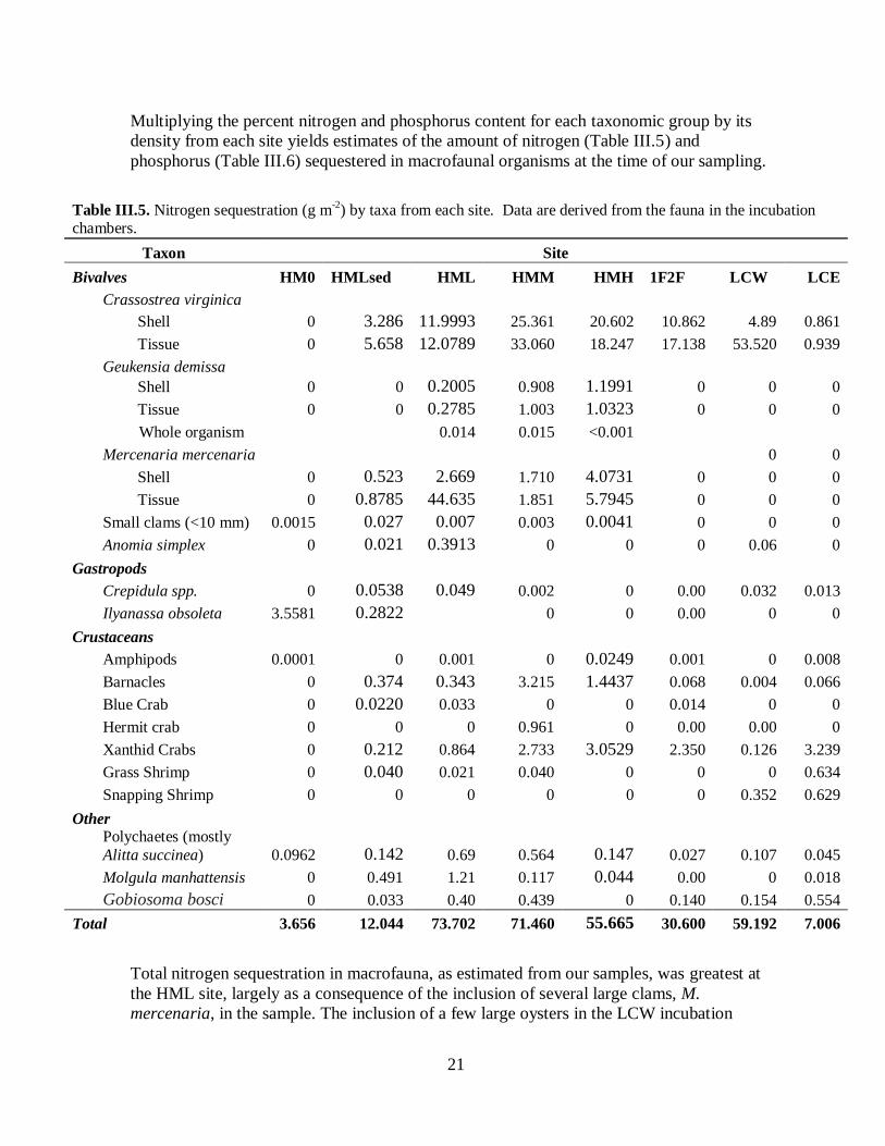
Multiplying the percent nitrogen and phosphorus content for each taxonomic group by its

density from each site yields estimates of the amount of nitrogen (Table III.5) and

phosphorus (Table III.6) sequestered in macrofaunal organisms at the time of our sampling.

Total nitrogen sequestration in macrofauna, as estimated from our samples, was greatest at

the HML site, largely as a consequence of the inclusion of several large clams, M.

mercenaria, in the sample. The inclusion of a few large oysters in the LCW incubation

Table III.5. Nitrogen sequestration (g m-2

) by taxa from each site. Data are derived from the fauna in the incubation chambers.

Taxon Site

Bivalves HM0 HMLsed HML HMM HMH 1F2F LCW LCE

Crassostrea virginica

Shell 0 3.286 11.9993 25.361 20.602 10.862 4.89 0.861

Tissue 0 5.658 12.0789 33.060 18.247 17.138 53.520 0.939

Geukensia demissa

Shell 0 0 0.2005 0.908 1.1991 0 0 0

Tissue 0 0 0.2785 1.003 1.0323 0 0 0

Whole organism 0.014 0.015 <0.001

Mercenaria mercenaria

0 0

Shell 0 0.523 2.669 1.710 4.0731 0 0 0

Tissue 0 0.8785 44.635 1.851 5.7945 0 0 0

Small clams (<10 mm) 0.0015 0.027 0.007 0.003 0.0041 0 0 0

Anomia simplex 0 0.021 0.3913 0 0 0 0.06 0

Gastropods

Crepidula spp. 0 0.0538 0.049 0.002 0 0.00 0.032 0.013

Ilyanassa obsoleta 3.5581 0.2822 0 0 0.00 0 0

Crustaceans

Amphipods 0.0001 0 0.001 0 0.0249 0.001 0 0.008

Barnacles 0 0.374 0.343 3.215 1.4437 0.068 0.004 0.066

Blue Crab 0 0.0220 0.033 0 0 0.014 0 0

Hermit crab 0 0 0 0.961 0 0.00 0.00 0

Xanthid Crabs 0 0.212 0.864 2.733 3.0529 2.350 0.126 3.239

Grass Shrimp 0 0.040 0.021 0.040 0 0 0 0.634

Snapping Shrimp 0 0 0 0 0 0 0.352 0.629

Other

Polychaetes (mostly

Alitta succinea) 0.0962 0.142 0.69 0.564 0.147 0.027 0.107 0.045

Molgula manhattensis 0 0.491 1.21 0.117 0.044 0.00 0 0.018

Gobiosoma bosci 0 0.033 0.40 0.439 0 0.140 0.154 0.554

Total 3.656 12.044 73.702 71.460 55.665 30.600 59.192 7.006

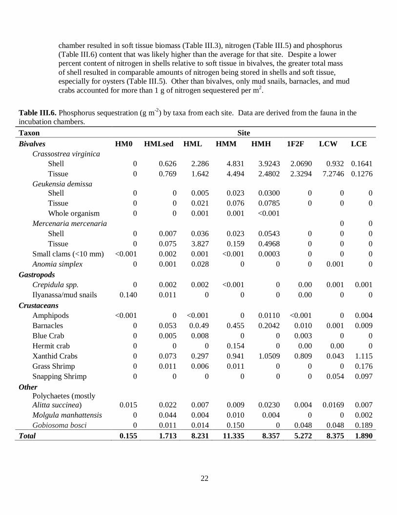
22

chamber resulted in soft tissue biomass (Table III.3), nitrogen (Table III.5) and phosphorus

(Table III.6) content that was likely higher than the average for that site. Despite a lower

percent content of nitrogen in shells relative to soft tissue in bivalves, the greater total mass

of shell resulted in comparable amounts of nitrogen being stored in shells and soft tissue,

especially for oysters (Table III.5). Other than bivalves, only mud snails, barnacles, and mud

crabs accounted for more than 1 g of nitrogen sequestered per m2.

Table III.6. Phosphorus sequestration (g m-2

) by taxa from each site. Data are derived from the fauna in the

incubation chambers.

Taxon Site

Bivalves HM0 HMLsed HML HMM HMH 1F2F LCW LCE

Crassostrea virginica

Shell 0 0.626 2.286 4.831 3.9243 2.0690 0.932 0.1641

Tissue 0 0.769 1.642 4.494 2.4802 2.3294 7.2746 0.1276

Geukensia demissa

Shell 0 0 0.005 0.023 0.0300 0 0 0

Tissue 0 0 0.021 0.076 0.0785 0 0 0

Whole organism 0 0 0.001 0.001 <0.001

Mercenaria mercenaria

0 0

Shell 0 0.007 0.036 0.023 0.0543 0 0 0

Tissue 0 0.075 3.827 0.159 0.4968 0 0 0

Small clams (<10 mm) <0.001 0.002 0.001 <0.001 0.0003 0 0 0

Anomia simplex 0 0.001 0.028 0 0 0 0.001 0

Gastropods

Crepidula spp. 0 0.002 0.002 <0.001 0 0.00 0.001 0.001

Ilyanassa/mud snails 0.140 0.011 0 0 0 0.00 0 0

Crustaceans

Amphipods <0.001 0 <0.001 0 0.0110 <0.001 0 0.004

Barnacles 0 0.053 0.0.49 0.455 0.2042 0.010 0.001 0.009

Blue Crab 0 0.005 0.008 0 0 0.003 0 0

Hermit crab 0 0 0 0.154 0 0.00 0.00 0

Xanthid Crabs 0 0.073 0.297 0.941 1.0509 0.809 0.043 1.115

Grass Shrimp 0 0.011 0.006 0.011 0 0 0 0.176

Snapping Shrimp 0 0 0 0 0 0 0.054 0.097

Other

Polychaetes (mostly

Alitta succinea) 0.015 0.022 0.007 0.009 0.0230 0.004 0.0169 0.007

Molgula manhattensis 0 0.044 0.004 0.010 0.004 0 0 0.002

Gobiosoma bosci 0 0.011 0.014 0.150 0 0.048 0.048 0.189

Total 0.155 1.713 8.231 11.335 8.357 5.272 8.375 1.890

23

Phosphorus sequestration patterns followed those observed for nitrogen with the highest

levels estimated for the HMM site and lower levels estimated for HML, HMH and LCW

(Table III.6). Importantly, even the two reef sites with the lowest phosphorus sequestration

(HMLsed and LCE) had an order of magnitude more phosphorus sequestered in macrofaunal

biomass than did the site without oysters (HM0).

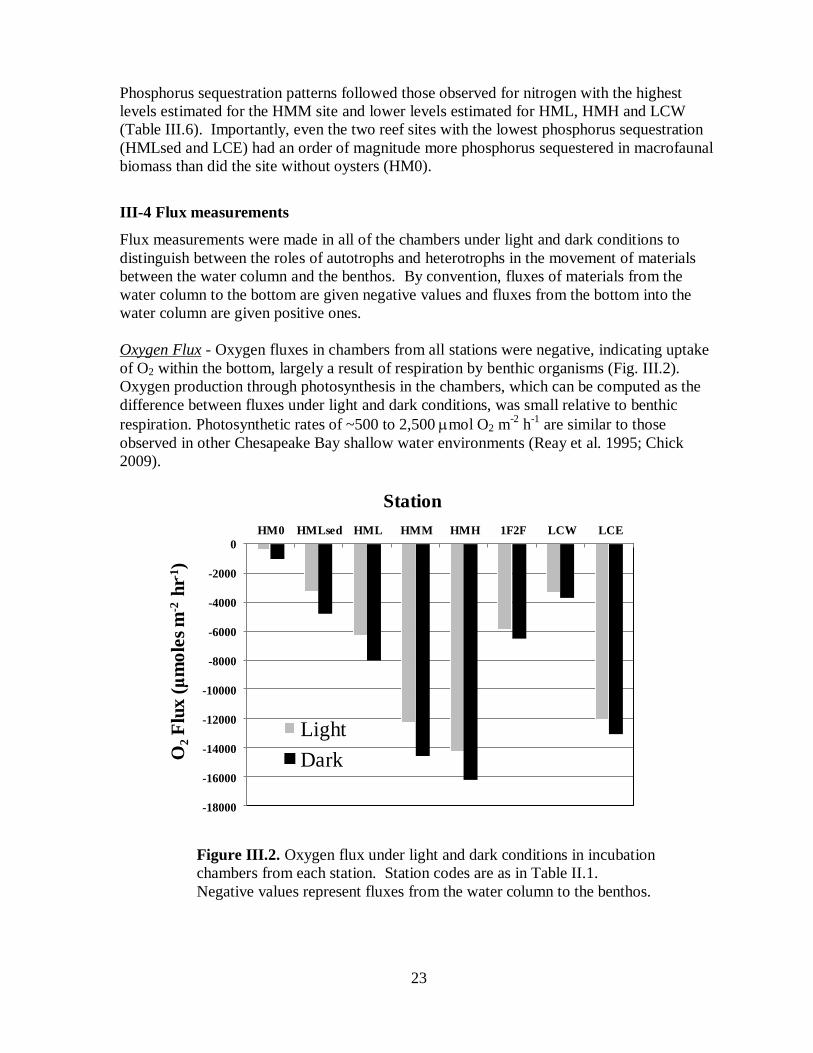
III-4 Flux measurements

Flux measurements were made in all of the chambers under light and dark conditions to

distinguish between the roles of autotrophs and heterotrophs in the movement of materials

between the water column and the benthos. By convention, fluxes of materials from the

water column to the bottom are given negative values and fluxes from the bottom into the

water column are given positive ones.

Oxygen Flux - Oxygen fluxes in chambers from all stations were negative, indicating uptake

of O2 within the bottom, largely a result of respiration by benthic organisms (Fig. III.2).

Oxygen production through photosynthesis in the chambers, which can be computed as the

difference between fluxes under light and dark conditions, was small relative to benthic

respiration. Photosynthetic rates of ~500 to 2,500 mol O2 m-2

h-1

are similar to those

observed in other Chesapeake Bay shallow water environments (Reay et al. 1995; Chick

2009).

Figure III.2. Oxygen flux under light and dark conditions in incubation

chambers from each station. Station codes are as in Table II.1.

Negative values represent fluxes from the water column to the benthos.

-18000

-16000

-14000

-12000

-10000

-8000

-6000

-4000

-2000

0

HM0 HMLsed HML HMM HMH 1F2F LCW LCE

O2

Flu

x (

μm

ole

s m

-2h

r-1)

Station

Light

Dark

24

Oxygen consumption in the Humes Marsh treatments increased monotonically with oyster

abundance and biomass measurements made at the field sites (compare values in Table III.1

to Humes Marsh treatments in Fig. III.2). There is not a similar clear relationship between

the other three stations, where the Long Creek East treatment had much higher fluxes than

the other two sites, despite having similar oyster abundances and biomass.

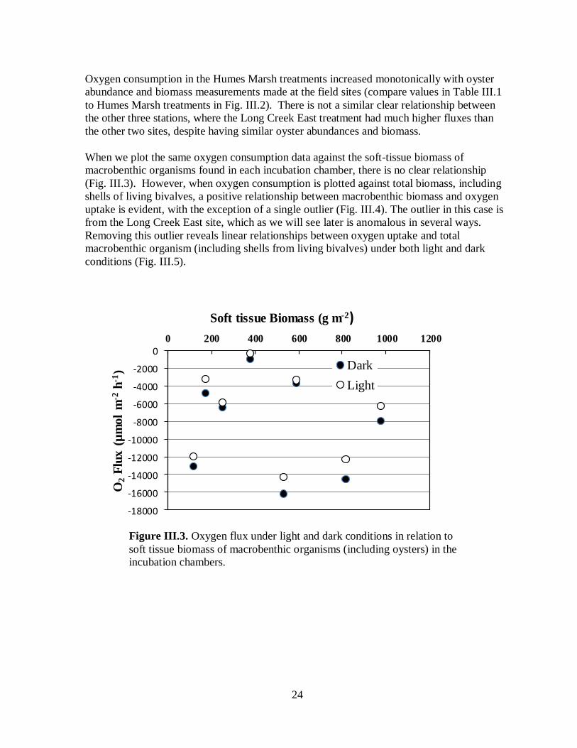
When we plot the same oxygen consumption data against the soft-tissue biomass of

macrobenthic organisms found in each incubation chamber, there is no clear relationship

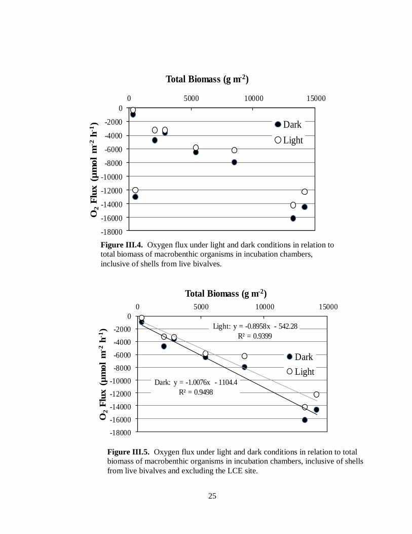
(Fig. III.3). However, when oxygen consumption is plotted against total biomass, including

shells of living bivalves, a positive relationship between macrobenthic biomass and oxygen

uptake is evident, with the exception of a single outlier (Fig. III.4). The outlier in this case is

from the Long Creek East site, which as we will see later is anomalous in several ways.

Removing this outlier reveals linear relationships between oxygen uptake and total

macrobenthic organism (including shells from living bivalves) under both light and dark

conditions (Fig. III.5).

Figure III.3. Oxygen flux under light and dark conditions in relation to

soft tissue biomass of macrobenthic organisms (including oysters) in the

incubation chambers.

-18000

-16000

-14000

-12000

-10000

-8000

-6000

-4000

-2000

00 200 400 600 800 1000 1200

O2

Flu

x (

µm

ol

m-2

h-1

)

Soft tissue Biomass (g m-2)

Dark

Light

25

Figure III.5. Oxygen flux under light and dark conditions in relation to total

biomass of macrobenthic organisms in incubation chambers, inclusive of shells

from live bivalves and excluding the LCE site.

Dark: y = -1.0076x - 1104.4

R² = 0.9498

Light: y = -0.8958x - 542.28

R² = 0.9399

-18000

-16000

-14000

-12000

-10000

-8000

-6000

-4000

-2000

0

0 5000 10000 15000

O2

Flu

x (

µm

ol

m-2

h-1

)

Total Biomass (g m-2)

Dark

Light

-18000

-16000

-14000

-12000

-10000

-8000

-6000

-4000

-2000

0

0 5000 10000 15000O

2F

lux (

µm

ol

m-2

h-1

)

Total Biomass (g m-2)

Dark

Light

Figure III.4. Oxygen flux under light and dark conditions in relation to

total biomass of macrobenthic organisms in incubation chambers,

inclusive of shells from live bivalves.

26

Ammonium nitrogen flux – Fluxes of nitrogen in the form of ammonium from the water

column to the benthos (negative fluxes) reflect uptake by macro- and micro-benthic algae.

Release of ammonium from the benthos into the water column reflects both direct release by

oysters and other macrofauna and remineralization of more complex organic nitrogen

biodeposits by microbes (see Fig. I.1). Uptake of ammonium by the benthos was observed

in only three of the incubation chambers under light conditions (Fig. III.6). The two site at

Humes Marsh with a soft sediment base and the Long Creek West site, which also lacked a

shell base, were observed to uptake NH4+ at rates between 103 and 288 μmoles m

-2 hr

-1 (Fig.

III.6). The highest rates observed here (> 1,000 μmoles m-2

hr-1

) are higher than observed

rates under anoxic conditions in the Chesapeake mid-bay region (Cowan and Boynton 1996)

but lower than summer rates in the Choptank River (Kellogg et al. 2011).

There is a weak positive relationship between ammonium flux and soft-tissue biomass,

inclusive of oysters, in the incubation chambers from each site (Fig. III.7). This relationship,

however, is much stronger when the biomass estimates include the shell from live bivalves

within the chambers, with over 90% and 94% of the variation in NH4+ measurements in light

and dark conditions, respectively, explained by the total macrofauna biomass within the

chambers (Fig. III.8). Interestingly, comparably good relationships were observed between

ammonium flux and the soft-tissue biomass from oysters measured at the field sites at the

time chamber base trays were deployed (Fig. III.9).

-500

0

500

1000

1500

2000

HM0 HMLsed HML HMM HMH 1F2F LCW LCE

NH

4+

Flu

x (

μm

ole

s m

-2h

r-1)

Station

Light

Dark

Figure III.6. Ammonium (NH4+) flux under light and dark

conditions in incubation chambers from each station. Negative

values represent fluxes from the water column to the benthos.

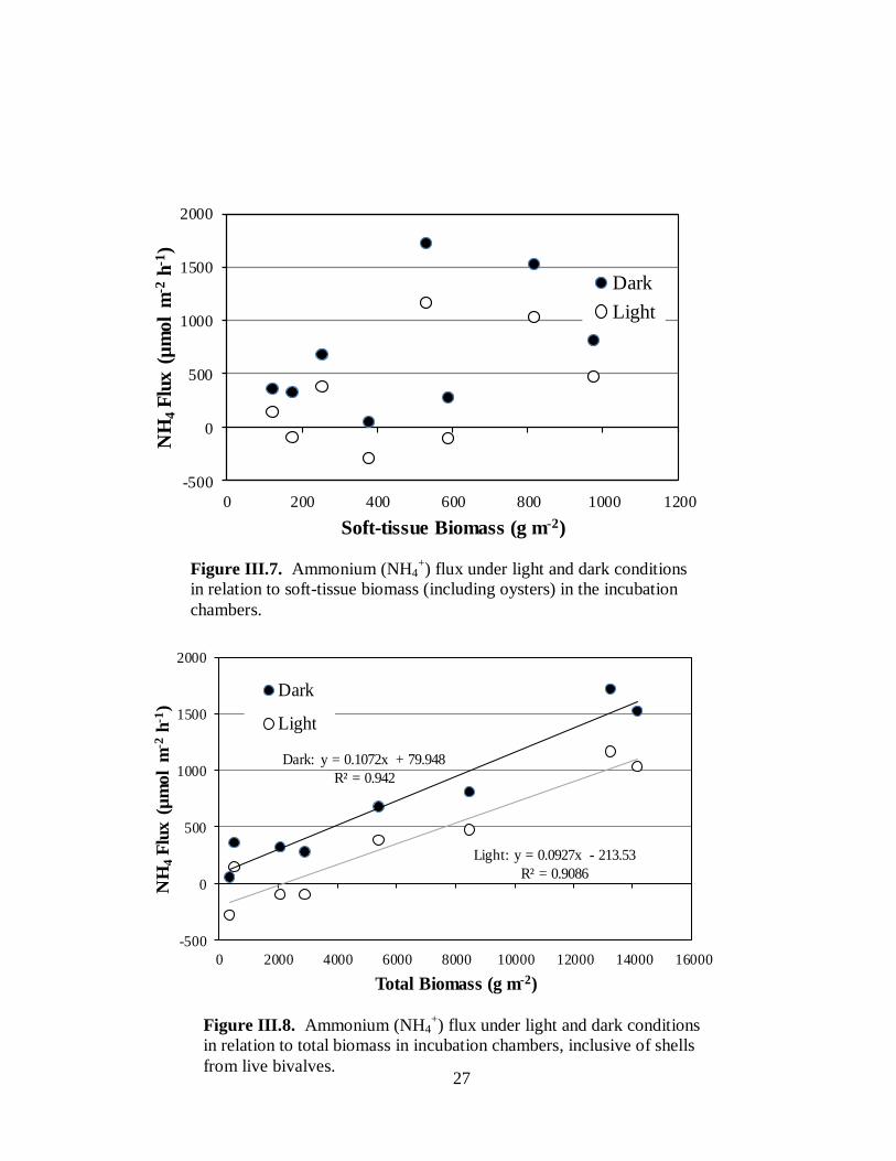
27

-500

0

500

1000

1500

2000

0 200 400 600 800 1000 1200

NH

4F

lux (

µm

ol

m-2

h-1

)

Soft-tissue Biomass (g m-2)

Dark

Light

Figure III.7. Ammonium (NH4+) flux under light and dark conditions

in relation to soft-tissue biomass (including oysters) in the incubation

chambers.

Dark: y = 0.1072x + 79.948

R² = 0.942

Light: y = 0.0927x - 213.53

R² = 0.9086

-500

0

500

1000

1500

2000

0 2000 4000 6000 8000 10000 12000 14000 16000

NH

4F

lux

(µ

mo

l m

-2h

-1)

Total Biomass (g m-2)

Dark

Light

Figure III.8. Ammonium (NH4+) flux under light and dark conditions

in relation to total biomass in incubation chambers, inclusive of shells

from live bivalves.

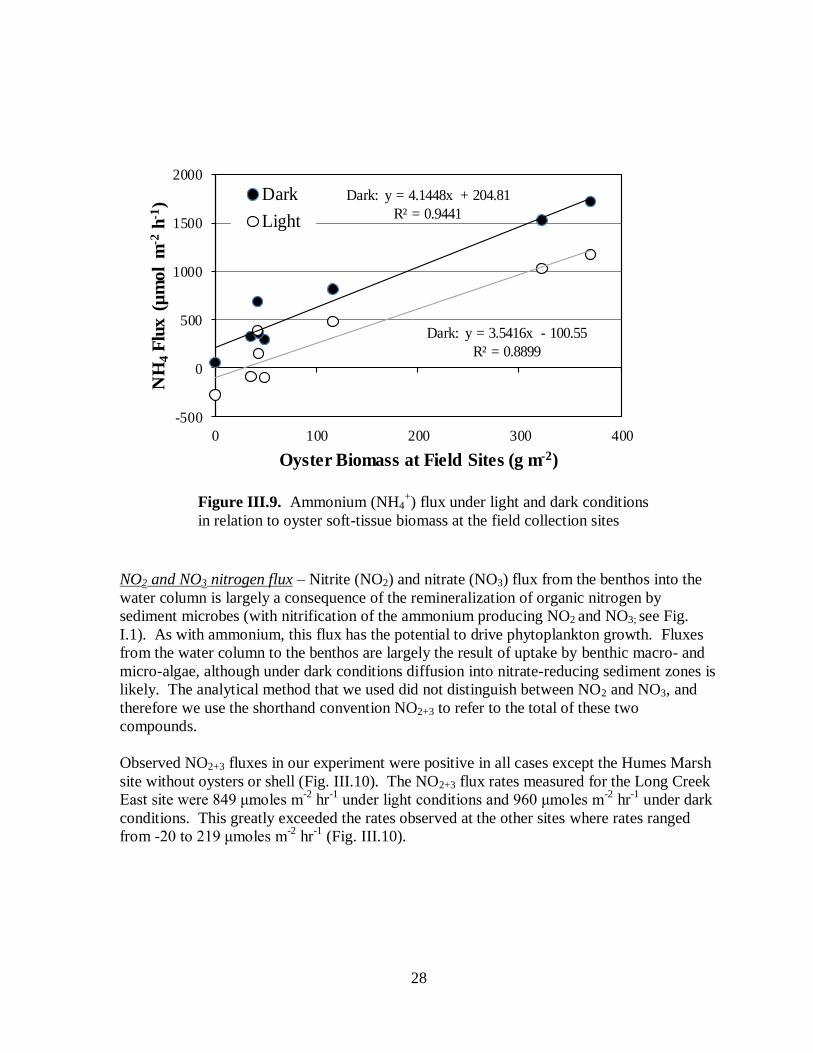
28

NO2 and NO3 nitrogen flux – Nitrite (NO2) and nitrate (NO3) flux from the benthos into the

water column is largely a consequence of the remineralization of organic nitrogen by

sediment microbes (with nitrification of the ammonium producing NO2 and NO3; see Fig.

I.1). As with ammonium, this flux has the potential to drive phytoplankton growth. Fluxes

from the water column to the benthos are largely the result of uptake by benthic macro- and

micro-algae, although under dark conditions diffusion into nitrate-reducing sediment zones is

likely. The analytical method that we used did not distinguish between NO2 and NO3, and

therefore we use the shorthand convention NO2+3 to refer to the total of these two

compounds.

Observed NO2+3 fluxes in our experiment were positive in all cases except the Humes Marsh

site without oysters or shell (Fig. III.10). The NO2+3 flux rates measured for the Long Creek

East site were 849 μmoles m-2

hr-1

under light conditions and 960 μmoles m-2

hr-1

under dark

conditions. This greatly exceeded the rates observed at the other sites where rates ranged

from -20 to 219 μmoles m-2

hr-1

(Fig. III.10).

Dark: y = 4.1448x + 204.81

R² = 0.9441

Dark: y = 3.5416x - 100.55

R² = 0.8899

-500

0

500

1000

1500

2000

0 100 200 300 400

NH

4F

lux

(µ

mo

l m

-2h

-1)

Oyster Biomass at Field Sites (g m-2)

Dark

Light

Figure III.9. Ammonium (NH4+) flux under light and dark conditions

in relation to oyster soft-tissue biomass at the field collection sites

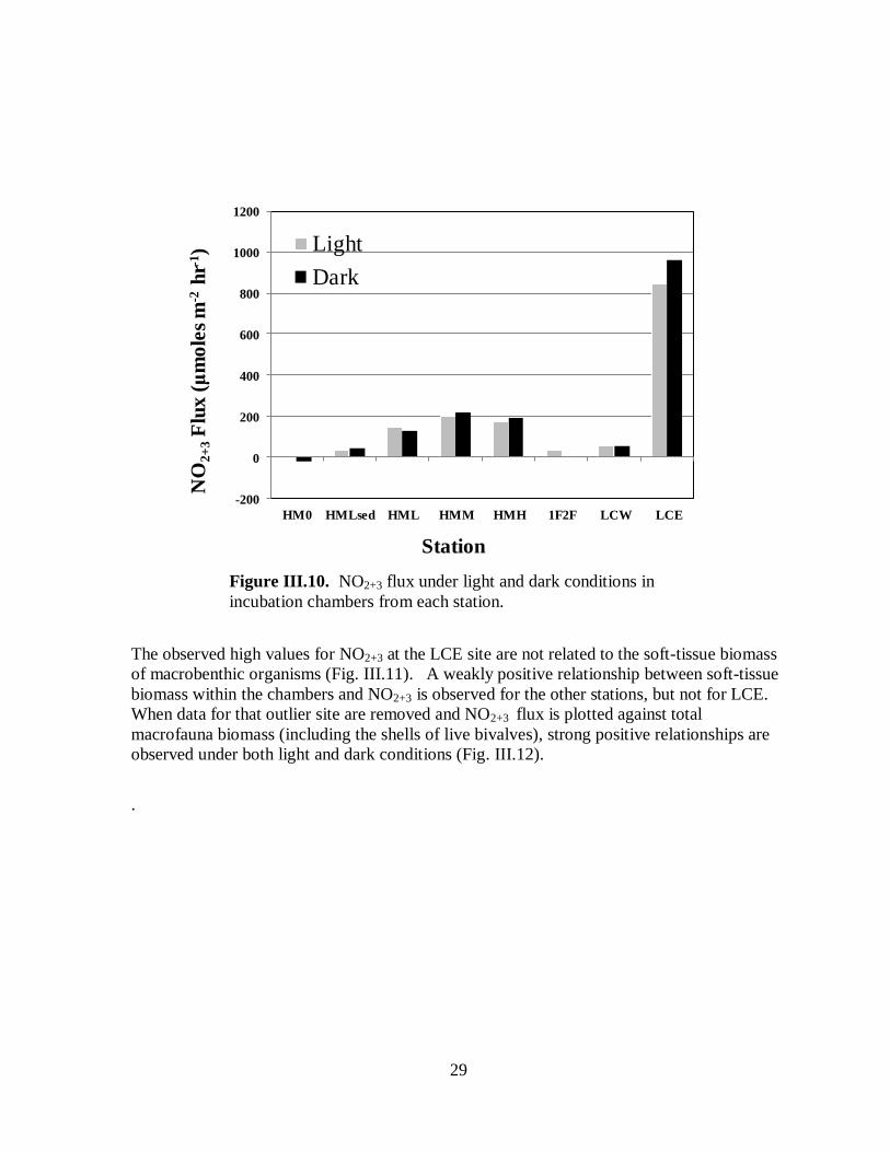
29

The observed high values for NO2+3 at the LCE site are not related to the soft-tissue biomass

of macrobenthic organisms (Fig. III.11). A weakly positive relationship between soft-tissue

biomass within the chambers and NO2+3 is observed for the other stations, but not for LCE.

When data for that outlier site are removed and NO2+3 flux is plotted against total

macrofauna biomass (including the shells of live bivalves), strong positive relationships are

observed under both light and dark conditions (Fig. III.12).

.

-200

0

200

400

600

800

1000

1200

HM0 HMLsed HML HMM HMH 1F2F LCW LCE

NO

2+

3F

lux (

μm

ole

s m

-2h

r-1)

Station

Light

Dark

Figure III.10. NO2+3 flux under light and dark conditions in

incubation chambers from each station.

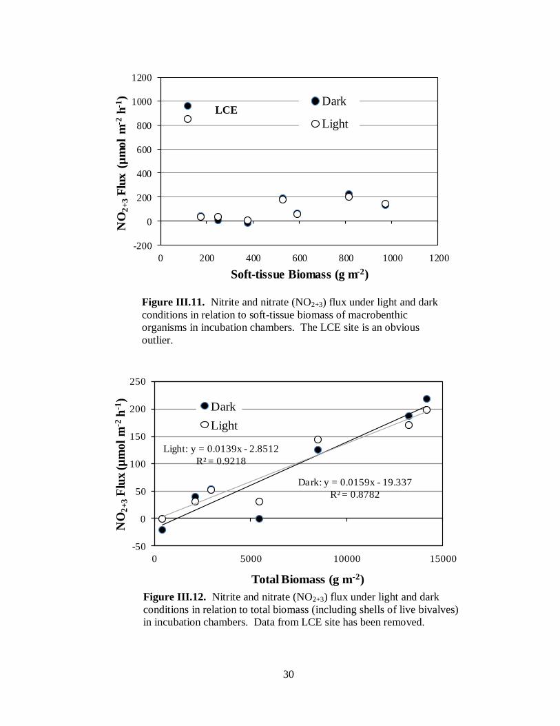
30

Dark: y = 0.0159x - 19.337

R² = 0.8782

Light: y = 0.0139x - 2.8512

R² = 0.9218

-50

0

50

100

150

200

250

0 5000 10000 15000

NO

2+

3F

lux

(µ

mo

l m

-2h

-1)

Total Biomass (g m-2)

Dark

Light

Figure III.12. Nitrite and nitrate (NO2+3) flux under light and dark

conditions in relation to total biomass (including shells of live bivalves)

in incubation chambers. Data from LCE site has been removed.

-200

0

200

400

600

800

1000

1200

0 200 400 600 800 1000 1200

NO

2+

3F

lux (

µm

ol

m-2

h-1

)

Soft-tissue Biomass (g m-2)

Dark

Light

Figure III.11. Nitrite and nitrate (NO2+3) flux under light and dark

conditions in relation to soft-tissue biomass of macrobenthic

organisms in incubation chambers. The LCE site is an obvious

outlier.

LCE

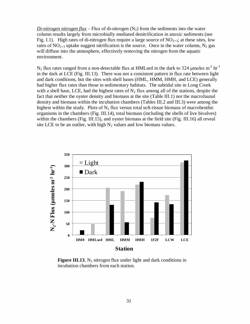
31

0

50

100

150

200

250

300

350

HM0 HMLsed HML HMM HMH 1F2F LCW LCE

N2-N

Flu

x (

μm

ole

s m

-2h

r-1)

Station

Light

Dark

Figure III.13. N2 nitrogen flux under light and dark conditions in

incubation chambers from each station.

Di-nitrogen nitrogen flux – Flux of di-nitrogen (N2) from the sediments into the water

column results largely from microbially mediated denitrification in anoxic sediments (see

Fig. I.1). High rates of di-nitrogen flux require a large source of NO2+3; at these sites, low

rates of NO2+3 uptake suggest nitrification is the source. Once in the water column, N2 gas

will diffuse into the atmosphere, effectively removing the nitrogen from the aquatic

environment.

N2 flux rates ranged from a non-detectable flux at HMLsed in the dark to 324 μmoles m-2

hr-1

in the dark at LCE (Fig. III.13). There was not a consistent pattern in flux rate between light

and dark conditions, but the sites with shell bases (HML, HMM, HMH, and LCE) generally

had higher flux rates than those in sedimentary habitats. The subtidal site in Long Creek

with a shell base, LCE, had the highest rates of N2 flux among all of the stations, despite the

fact that neither the oyster density and biomass at the site (Table III.1) nor the macrofaunal

density and biomass within the incubation chambers (Tables III.2 and III.3) were among the

highest within the study. Plots of N2 flux versus total soft-tissue biomass of macrobenthic

organisms in the chambers (Fig. III.14), total biomass (including the shells of live bivalves)

within the chambers (Fig. III.15), and oyster biomass at the field site (Fig. III.16) all reveal

site LCE to be an outlier, with high N2 values and low biomass values.

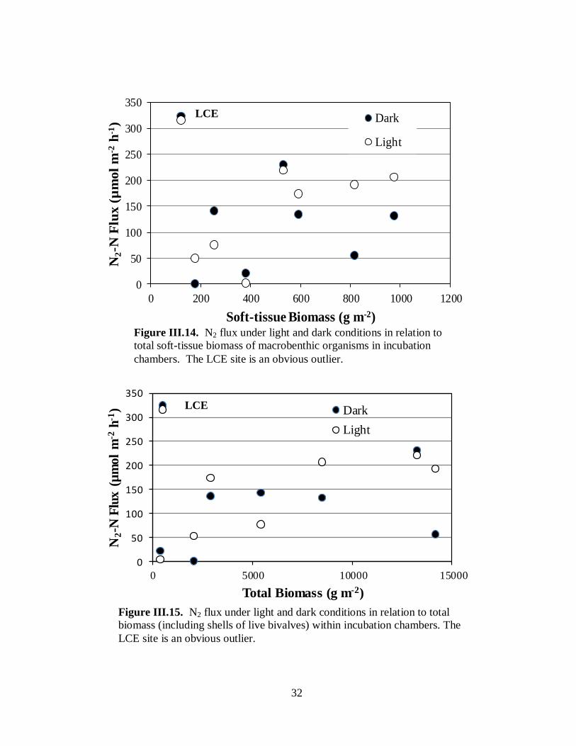
32

0

50

100

150

200

250

300

350

0 200 400 600 800 1000 1200

N2-N

Flu

x (

µm

ol

m-2

h-1

)

Soft-tissue Biomass (g m-2)

Dark

Light

LCE

Figure III.14. N2 flux under light and dark conditions in relation to

total soft-tissue biomass of macrobenthic organisms in incubation

chambers. The LCE site is an obvious outlier.

0

50

100

150

200

250

300

350

0 5000 10000 15000

N2-N

Flu

x (

µm

ol

m-2

h-1

)

Total Biomass (g m-2)

Dark

Light

Figure III.15. N2 flux under light and dark conditions in relation to total

biomass (including shells of live bivalves) within incubation chambers. The

LCE site is an obvious outlier.

LCE

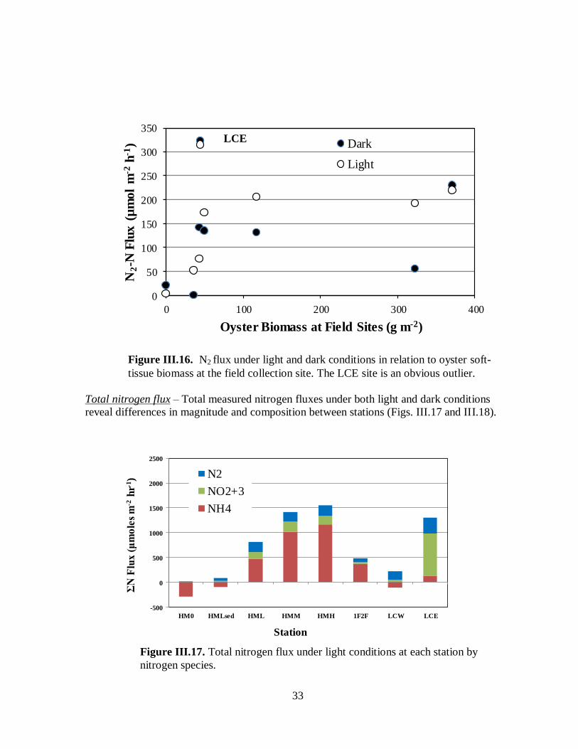
33

Total nitrogen flux – Total measured nitrogen fluxes under both light and dark conditions

reveal differences in magnitude and composition between stations (Figs. III.17 and III.18).

0

50

100

150

200

250

300

350

0 100 200 300 400

N2-N

Flu

x (

µm

ol

m-2

h-1

)

Oyster Biomass at Field Sites (g m-2)

Dark

Light

Figure III.16. N2 flux under light and dark conditions in relation to oyster soft-

tissue biomass at the field collection site. The LCE site is an obvious outlier.

LCE

-500

0

500

1000

1500

2000

2500

HM0 HMLsed HML HMM HMH 1F2F LCW LCE

ΣN

Flu

x (

μm

ole

s m

-2h

r-1)

Station

N2

NO2+3

NH4

Figure III.17. Total nitrogen flux under light conditions at each station by

nitrogen species.

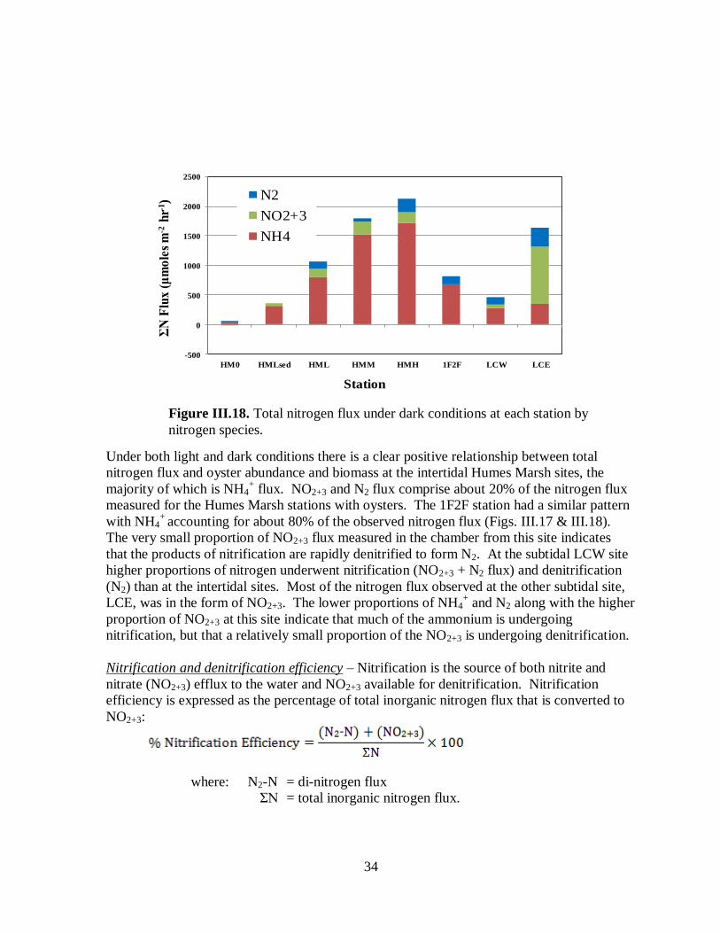
34

Under both light and dark conditions there is a clear positive relationship between total

nitrogen flux and oyster abundance and biomass at the intertidal Humes Marsh sites, the

majority of which is NH4+ flux. NO2+3 and N2 flux comprise about 20% of the nitrogen flux

measured for the Humes Marsh stations with oysters. The 1F2F station had a similar pattern

with NH4+

accounting for about 80% of the observed nitrogen flux (Figs. III.17 & III.18).

The very small proportion of NO2+3 flux measured in the chamber from this site indicates

that the products of nitrification are rapidly denitrified to form N2. At the subtidal LCW site

higher proportions of nitrogen underwent nitrification (NO2+3 + N2 flux) and denitrification

(N2) than at the intertidal sites. Most of the nitrogen flux observed at the other subtidal site,

LCE, was in the form of NO2+3. The lower proportions of NH4+ and N2 along with the higher

proportion of NO2+3 at this site indicate that much of the ammonium is undergoing

nitrification, but that a relatively small proportion of the NO2+3 is undergoing denitrification.

Nitrification and denitrification efficiency – Nitrification is the source of both nitrite and

nitrate (NO2+3) efflux to the water and NO2+3 available for denitrification. Nitrification

efficiency is expressed as the percentage of total inorganic nitrogen flux that is converted to

NO2+3:

where: N2-N = di-nitrogen flux

ΣN = total inorganic nitrogen flux.

Figure III.18. Total nitrogen flux under dark conditions at each station by

nitrogen species.

-500

0

500

1000

1500

2000

2500

HM0 HMLsed HML HMM HMH 1F2F LCW LCE

ΣN

Flu

x (

μm

ole

s m

-2h

r-1)

Station

N2

NO2+3

NH4

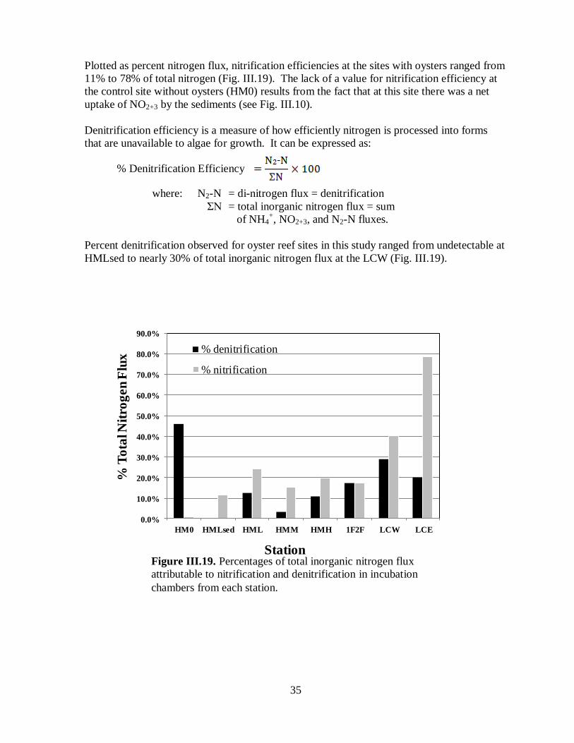
35

Plotted as percent nitrogen flux, nitrification efficiencies at the sites with oysters ranged from

11% to 78% of total nitrogen (Fig. III.19). The lack of a value for nitrification efficiency at

the control site without oysters (HM0) results from the fact that at this site there was a net

uptake of NO2+3 by the sediments (see Fig. III.10).

Denitrification efficiency is a measure of how efficiently nitrogen is processed into forms

that are unavailable to algae for growth. It can be expressed as:

where: N2-N = di-nitrogen flux = denitrification

ΣN = total inorganic nitrogen flux = sum

of NH4+, NO2+3, and N2-N fluxes.

Percent denitrification observed for oyster reef sites in this study ranged from undetectable at

HMLsed to nearly 30% of total inorganic nitrogen flux at the LCW (Fig. III.19).

0.0%

10.0%

20.0%

30.0%

40.0%

50.0%

60.0%

70.0%

80.0%

90.0%

HM0 HMLsed HML HMM HMH 1F2F LCW LCE

% T

ota

l Nit

rog

en

Flu

x

Station

% denitrification

% nitrification

Figure III.19. Percentages of total inorganic nitrogen flux

attributable to nitrification and denitrification in incubation

chambers from each station.

% Denitrification Efficiency

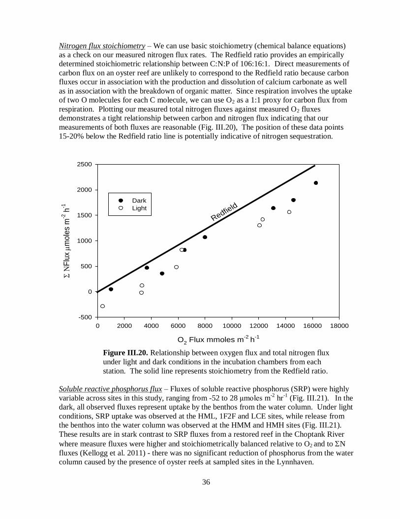
36

Nitrogen flux stoichiometry – We can use basic stoichiometry (chemical balance equations)

as a check on our measured nitrogen flux rates. The Redfield ratio provides an empirically

determined stoichiometric relationship between C:N:P of 106:16:1. Direct measurements of

carbon flux on an oyster reef are unlikely to correspond to the Redfield ratio because carbon

fluxes occur in association with the production and dissolution of calcium carbonate as well

as in association with the breakdown of organic matter. Since respiration involves the uptake

of two O molecules for each C molecule, we can use O2 as a 1:1 proxy for carbon flux from

respiration. Plotting our measured total nitrogen fluxes against measured O2 fluxes

demonstrates a tight relationship between carbon and nitrogen flux indicating that our

measurements of both fluxes are reasonable (Fig. III.20), The position of these data points

15-20% below the Redfield ratio line is potentially indicative of nitrogen sequestration.

O2 Flux mmoles m

-2 h

-1

0 2000 4000 6000 8000 10000 12000 14000 16000 18000

Flu

x m

ole

s m

-2 h

-1

-500

0

500

1000

1500

2000

2500

Dark

Light

Redfield

Soluble reactive phosphorus flux – Fluxes of soluble reactive phosphorus (SRP) were highly

variable across sites in this study, ranging from -52 to 28 μmoles m-2

hr-1

(Fig. III.21). In the

dark, all observed fluxes represent uptake by the benthos from the water column. Under light

conditions, SRP uptake was observed at the HML, 1F2F and LCE sites, while release from

the benthos into the water column was observed at the HMM and HMH sites (Fig. III.21).

These results are in stark contrast to SRP fluxes from a restored reef in the Choptank River

where measure fluxes were higher and stoichiometrically balanced relative to O2 and to N

fluxes (Kellogg et al. 2011) - there was no significant reduction of phosphorus from the water

column caused by the presence of oyster reefs at sampled sites in the Lynnhaven.

Figure III.20. Relationship between oxygen flux and total nitrogen flux

under light and dark conditions in the incubation chambers from each

station. The solid line represents stoichiometry from the Redfield ratio.

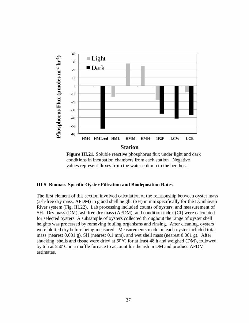
37

III-5 Biomass-Specific Oyster Filtration and Biodeposition Rates

The first element of this section involved calculation of the relationship between oyster mass

(ash-free dry mass, AFDM) in g and shell height (SH) in mm specifically for the Lynnhaven

River system (Fig. III.22). Lab processing included counts of oysters, and measurement of

SH. Dry mass (DM), ash free dry mass (AFDM), and condition index (CI) were calculated

for selected oysters. A subsample of oysters collected throughout the range of oyster shell

heights was processed by removing fouling organisms and rinsing. After cleaning, oysters

were blotted dry before being measured. Measurements made on each oyster included total

mass (nearest 0.001 g), SH (nearest 0.1 mm), and wet shell mass (nearest 0.001 g). After

shucking, shells and tissue were dried at 60°C for at least 48 h and weighed (DM), followed

by 6 h at 550°C in a muffle furnace to account for the ash in DM and produce AFDM

estimates.

-60

-50

-40

-30

-20

-10

0

10

20

30

40

HM0 HMLsed HML HMM HMH 1F2F LCW LCEPh

osp

ho

rus

Flu

x (

μm

ole

s m

-2h

r-1)

Station

Light

Dark

Figure III.21. Soluble reactive phosphorus flux under light and dark

conditions in incubation chambers from each station. Negative

values represent fluxes from the water column to the benthos.

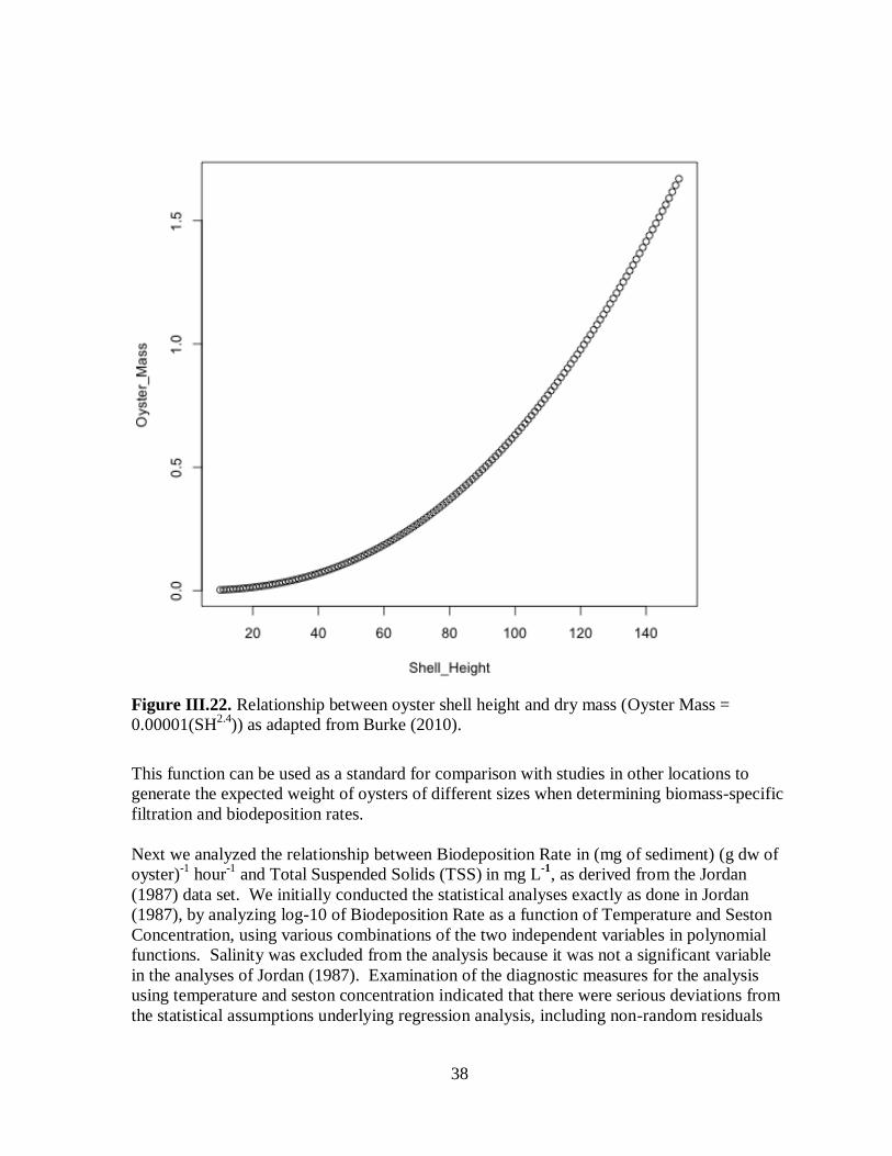
38

Figure III.22. Relationship between oyster shell height and dry mass (Oyster Mass =

0.00001(SH2.4

)) as adapted from Burke (2010).

This function can be used as a standard for comparison with studies in other locations to

generate the expected weight of oysters of different sizes when determining biomass-specific

filtration and biodeposition rates.

Next we analyzed the relationship between Biodeposition Rate in (mg of sediment) (g dw of

oyster)-1

hour-1

and Total Suspended Solids (TSS) in mg L-1

, as derived from the Jordan

(1987) data set. We initially conducted the statistical analyses exactly as done in Jordan

(1987), by analyzing log-10 of Biodeposition Rate as a function of Temperature and Seston

Concentration, using various combinations of the two independent variables in polynomial

functions. Salinity was excluded from the analysis because it was not a significant variable

in the analyses of Jordan (1987). Examination of the diagnostic measures for the analysis

using temperature and seston concentration indicated that there were serious deviations from

the statistical assumptions underlying regression analysis, including non-random residuals

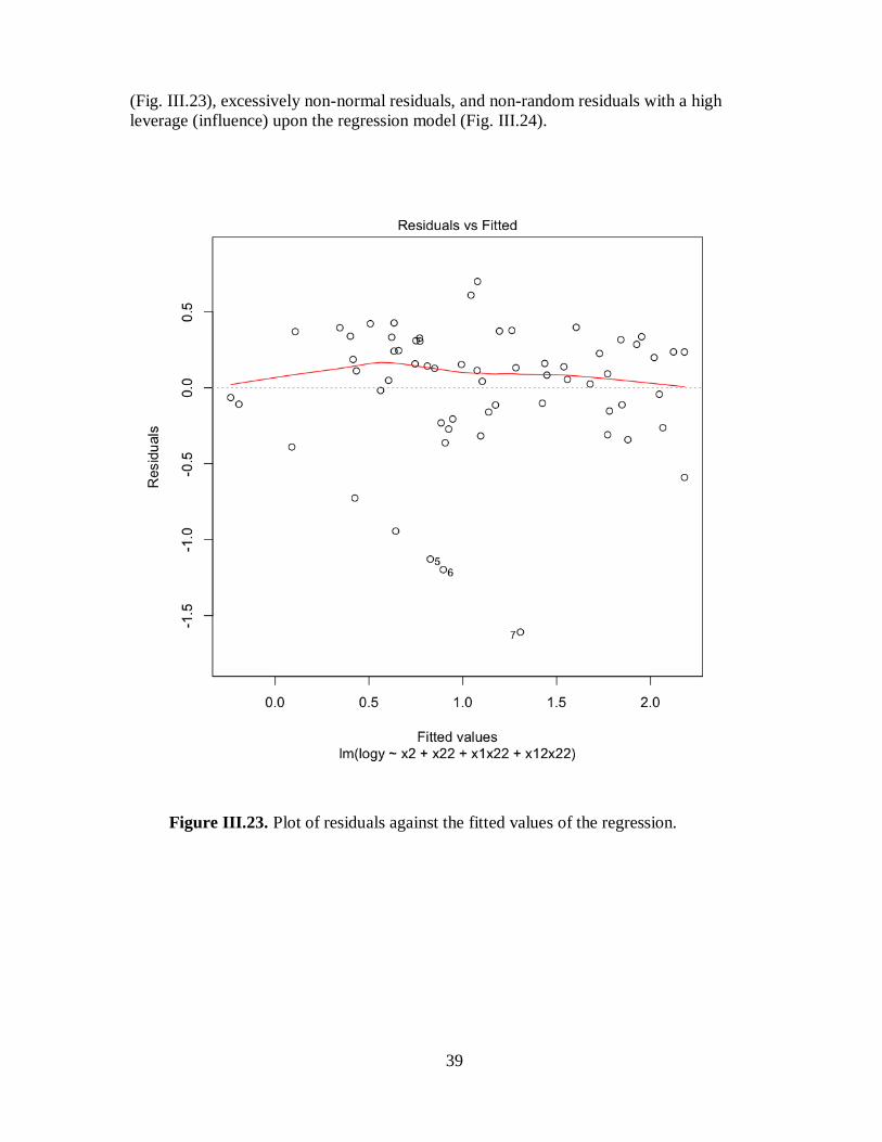
39

(Fig. III.23), excessively non-normal residuals, and non-random residuals with a high

leverage (influence) upon the regression model (Fig. III.24).

Figure III.23. Plot of residuals against the fitted values of the regression.

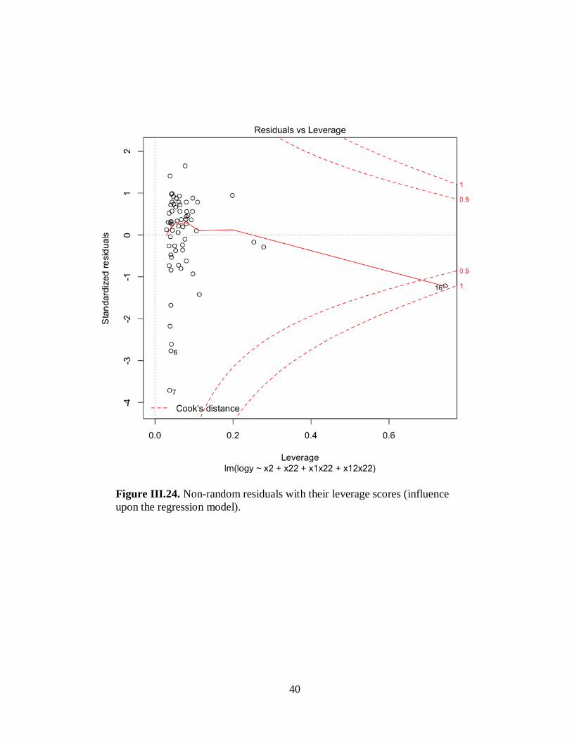
40

Figure III.24. Non-random residuals with their leverage scores (influence

upon the regression model).

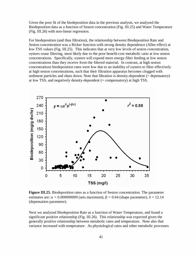
41

Given the poor fit of the biodeposition data in the previous analysis, we analyzed the

Biodeposition data as a function of Seston concentration (Fig. III.25) and Water Temperature

(Fig. III.26) with non-linear regression.

For biodeposition (and thus filtration), the relationship between Biodeposition Rate and

Seston concentration was a Ricker function with strong density dependence (Allee effect) at

low TSS values (Fig. III.25). This indicates that at very low levels of seston concentration,

oysters cease filtering, most likely due to the poor benefit:cost metabolic ratio at low seston

concentrations. Specifically, oysters will expend more energy filter feeding at low seston

concentrations than they receive from the filtered material. In contrast, at high seston

concentrations biodeposition rates were low due to an inability of oysters to filter effectively

at high seston concentrations, such that their filtration apparatus becomes clogged with

sediment particles and shuts down. Note that filtration is density-dependent (= depensatory)

at low TSS, and negatively density-dependent (= compensatory) at high TSS.

Figure III.25. Biodeposition rates as a function of Seston concentration. The parameter

estimates are: = 0.000000009 (sets maximum), = 0.64 (shape parameter), = 12.14

(depensation parameter).

Next we analyzed Biodeposition Rate as a function of Water Temperature, and found a

significant positive relationship (Fig. III.26). This relationship was expected given the

generally positive relationship between metabolic rates and temperature. Note also that

variance increased with temperature. As physiological rates and other metabolic processes

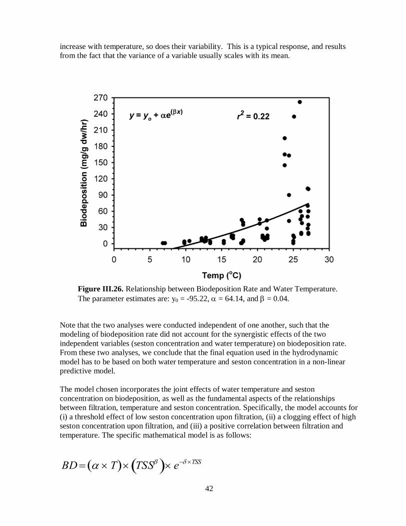
42

increase with temperature, so does their variability. This is a typical response, and results

from the fact that the variance of a variable usually scales with its mean.

Note that the two analyses were conducted independent of one another, such that the

modeling of biodeposition rate did not account for the synergistic effects of the two

independent variables (seston concentration and water temperature) on biodeposition rate.

From these two analyses, we conclude that the final equation used in the hydrodynamic

model has to be based on both water temperature and seston concentration in a non-linear

predictive model.

The model chosen incorporates the joint effects of water temperature and seston

concentration on biodeposition, as well as the fundamental aspects of the relationships

between filtration, temperature and seston concentration. Specifically, the model accounts for

(i) a threshold effect of low seston concentration upon filtration, (ii) a clogging effect of high

seston concentration upon filtration, and (iii) a positive correlation between filtration and

temperature. The specific mathematical model is as follows:

BD T TSS e TSS

Figure III.26. Relationship between Biodeposition Rate and Water Temperature.

The parameter estimates are: y0 = -95.22, = 64.14, and = 0.04.

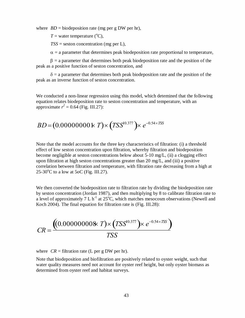
43

where BD = biodeposition rate (mg per g DW per hr),

T = water temperature (oC),

TSS = seston concentration (mg per L),

= a parameter that determines peak biodeposition rate proportional to temperature,

= a parameter that determines both peak biodeposition rate and the position of the

peak as a positive function of seston concentration, and

= a parameter that determines both peak biodeposition rate and the position of the

peak as an inverse function of seston concentration.

We conducted a non-linear regression using this model, which detemined that the following

equation relates biodeposition rate to seston concentration and temperature, with an

approximate r2 = 0.64 (Fig. III.27):

BD 0.000000001 T TSS10.377 e0.54TSS

Note that the model accounts for the three key characteristics of filtration: (i) a threshold

effect of low seston concentration upon filtration, whereby filtration and biodeposition

become negligible at seston concentrations below about 5-10 mg/L, (ii) a clogging effect

upon filtration at high seston concentrations greater than 20 mg/L, and (iii) a positive

correlation between filtration and temperature, with filtration rate decreasing from a high at

25-30oC to a low at 5oC (Fig. III.27).

We then converted the biodeposition rate to filtration rate by dividing the biodeposition rate

by seston concentration (Jordan 1987), and then multiplying by 8 to calibrate filtration rate to

a level of approximately 7 L h-1

at 25oC, which matches mesocosm observations (Newell and

Koch 2004). The final equation for filtration rate is (Fig. III.28):

CR 0.000000008T TSS10.377 e0.54TSS

TSS

where CR = filtration rate (L per g DW per hr).

Note that biodeposition and biofiltration are positively related to oyster weight, such that

water quality measures need not account for oyster reef height, but only oyster biomass as

determined from oyster reef and habitat surveys.

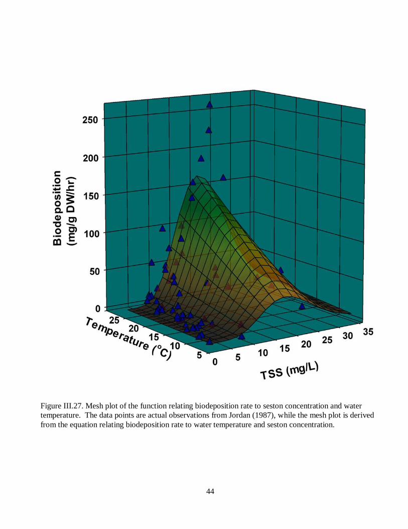
44

Figure III.27. Mesh plot of the function relating biodeposition rate to seston concentration and water

temperature. The data points are actual observations from Jordan (1987), while the mesh plot is derived

from the equation relating biodeposition rate to water temperature and seston concentration.

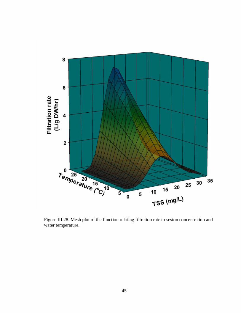
45

Figure III.28. Mesh plot of the function relating filtration rate to seston concentration and

water temperature.

46

CHAPTER IV. SUMMARY AND CONCLUSIONS

Through their filtration activity, oysters remove phytoplankton, sediments, and other

suspended particles from the water column. The fate of these materials and the associated

nutrients depends upon physical, chemical and biological factors in the environment.

Sediments deposited on the bottom may be resuspended, temporarily buried, or incorporated

more deeply into the reef matrix, resulting in longer-term burial. A portion of the ingested

nutrients become incorporated into the soft tissues and shell of the oyster. If the oyster is

subsequently harvested, these nutrients will be removed from the water body. If the oyster is

not removed from the water, then the nutrients within the soft tissue are eventually recycled

through the system when the oyster dies. Nutrients sequestered within the shell matrix are

effectively removed from the water body for a longer period of time. A portion of the

nitrogen ingested by oysters is excreted directly back into the water column in the form of

ammonium (NH4+) where it is available for uptake by phytoplankton and macroalgae.

Finally, oyster biodeposits (feces and pseudofeces) contain organic nitrogen and phosphorus.

Once on the bottom, phosphorus dynamics are heavily influenced by sediment chemistry and

in general are poorly characterized. Nitrogen dynamics are also complex and largely driven

by microbial activity. Through a series of processes termed nitrification organic nitrogen is

transformed via the action of aerobic microbes to NH4+, NO2 and NO3, all of which may be

released from the sediments and support the growth of benthic microalgae and macroalgae

and phytoplankton (see Fig. I.1). Under the proper conditions a portion of the NO2 and NO3

may be converted by anaerobic bacteria to N2 gas that escapes from the water column into

the atmosphere.

This study represents a first attempt to quantify the fate of some of these materials, primarily

nutrients, as they cycle through oyster reefs in the Lynnhaven River. Fully quantifying the

fate of materials processed by oyster throughout the Lynnhaven will require long-term

seasonal rate measurements across a wide range of environmental conditions coupled with

dynamic water quality modeling. Though this scale of effort was beyond the scope of this

project, our findings reveal much about the effects of oyster reefs in the Lynnhaven River on

the fate of nutrients, especially nitrogen, within the system.

The sites for which we characterized nutrient dynamics in the Lynnhaven River vary in

oyster abundance, oyster biomass, substratum characteristics, and tidal emersion. At the

intertidal sites located at Humes Marsh, we observed strong, linear relationships between

oyster biomass in the field and O2, NH4+, and NO2+3 fluxes in the incubation chambers. We

observed similar relationships between these fluxes and total faunal biomass in the

incubation chambers, but only when shell biomass from living oysters was included in the

calculation. Two of the Long Creek stations (1F2F and LCW) also fit this pattern of strong

relationships between biomass and fluxes of O2, NH4+, and NO2+3. The One Fish-Two Fish

site is intertidal, sandy-mud bottom with a low density of oysters, while the Long Creek West

site is a subtidal, sandy-mud bottom with a low density of oysters. The one site that was

consistently an outlier in these relationships was LCE, a subtidal site with a shell base bottom

and a low density of oysters. We discuss possible reasons for the divergent responses at this

site later in this section.

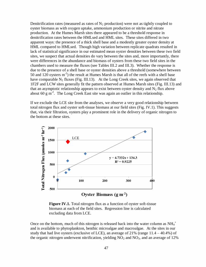
47

Denitrification rates (measured as rates of N2 production) were not as tightly coupled to

oyster biomass as with oxygen uptake, ammonium production or nitrite and nitrate

production. At the Humes Marsh sites there appeared to be a threshold response in

denitrification rates between the HMLsed and HML sites. These sites differed in two

apparent ways: the presence of a thick shell base and a modestly greater oyster density at

HML compared to HMLsed. Though high variation between replicate quadrats resulted in

lack of statistical significance in our estimated mean oyster densities between these two field

sites, we suspect that actual densities do vary between the sites and, more importantly, there

were differences in the abundance and biomass of oysters from these two field sites in the

chambers used to measure the fluxes (see Tables III.2 and III.3). Whether the response is

due to the presence of a shell base or oyster densities above a threshold (somewhere between

50 and 120 oysters m-2

) the result at Humes Marsh is that all of the reefs with a shell base

have comparable N2 fluxes (Fig. III.13). At the Long Creek sites, we again observed that

1F2F and LCW sites generally fit the pattern observed at Humes Marsh sites (Fig. III.13) and

that an asymptotic relationship appears to exist between oyster density and N2 flux above

about 60 g m-2

. The Long Creek East site was again an outlier in this relationship.

If we exclude the LCE site from the analyses, we observe a very good relationship between

total nitrogen flux and oyster soft-tissue biomass at our field sites (Fig. IV.1). This suggests

that, via their filtration, oysters play a prominent role in the delivery of organic nitrogen to

the bottom at these sites.

Once on the bottom, much of this nitrogen is released back into the water column as NH4+

and is available to phytoplankton, benthic microalgae and macroalgae. At the sites in our

study that had live oysters (exclusive of LCE), an average of 21% (range 11.4 – 40.4%) of

the organic nitrogen underwent nitrification, yielding NO2 and NO3, and an average of 12%

Figure IV.1. Total nitrogen flux as a function of oyster soft-tissue

biomass at each of the field sites. Regression line is calculated

excluding data from LCE.

LCE

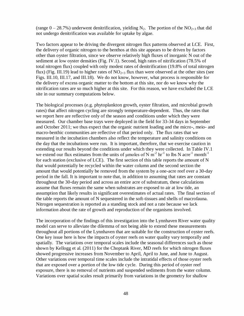
48

(range 0 – 28.7%) underwent denitrification, yielding N2. The portion of the NO2+3 that did

not undergo denitrification was available for uptake by algae.

Two factors appear to be driving the divergent nitrogen flux patterns observed at LCE. First,

the delivery of organic nitrogen to the benthos at this site appears to be driven by factors

other than oyster filtration, since we observe relatively high fluxes of inorganic N out of the

sediment at low oyster densities (Fig. IV.1). Second, high rates of nitrification (78.5% of

total nitrogen flux) coupled with only modest rates of denitrification (19.8% of total nitrogen

flux) (Fig. III.19) lead to higher rates of NO2+3 flux than were observed at the other sites (see

Figs. III.10, III.17, and III.18). We do not know, however, what process is responsible for

the delivery of excess organic matter to the bottom at this site, nor do we know why the

nitrification rates are so much higher at this site. For this reason, we have excluded the LCE

site in our summary computations below.

The biological processes (e.g. phytoplankton growth, oyster filtration, and microbial growth

rates) that affect nitrogen cycling are strongly temperature-dependent. Thus, the rates that

we report here are reflective only of the season and conditions under which they were

measured. Our chamber base trays were deployed in the field for 33-34 days in September

and October 2011; we thus expect that the organic nutrient loading and the micro-, meio- and

macro-benthic communities are reflective of that period only. The flux rates that we

measured in the incubation chambers also reflect the temperature and salinity conditions on

the day that the incubations were run. It is important, therefore, that we exercise caution in

extending our results beyond the conditions under which they were collected. In Table IV.1

we extend our flux estimates from the units of μmoles of N m-2

hr-1

to lbs N acre-1

month-1

for each station (exclusive of LCE). The first section of this table reports the amount of N

that would potentially be recycled within the water column and the second section the

amount that would potentially be removed from the system by a one-acre reef over a 30-day

period in the fall. It is important to note that, in addition to assuming that rates are constant

throughout the 30-day period and across an entire acre of substratum, these calculations

assume that fluxes remain the same when substrates are exposed to air at low tide, an

assumption that likely results in significant overestimates of actual rates. The final section of

the table reports the amount of N sequestered in the soft-tissues and shells of macrofauna.

Nitrogen sequestration is reported as a standing stock and not a rate because we lack

information about the rate of growth and reproduction of the organisms involved.

The incorporation of the findings of this investigation into the Lynnhaven River water quality

model can serve to alleviate the dilemma of not being able to extend these measurements

throughout all portions of the Lynnhaven that are suitable for the construction of oyster reefs.

One key issue here is how the impacts of oyster reefs on water quality vary temporally and

spatially. The variations over temporal scales include the seasonal differences such as those

shown by Kellogg et al. (2011) for the Choptank River, MD reefs for which nitrogen fluxes

showed progressive increases from November to April, April to June, and June to August.

Other variations over temporal time scales include the intratidal effects of those oyster reefs

that are exposed over a portion of the low tide cycle. During this period of oyster reef

exposure, there is no removal of nutrients and suspended sediments from the water column.

Variations over spatial scales result primarily from variations in the geometry for shallow

49

water regions such as the Lynnhaven. The suitability for optimal growth from oyster reefs is

dependent on factors such as local bathymetry as well as water quality conditions.

The goal of this study was to provide estimates of (1) oyster filtration rates, (2) biodeposition

rates, (3) nutrient flux rates between the sediment and water column, and (4) nutrient

sequestration in relation to oyster biomass on reefs in the Lynnhaven River, with the intent

that these would then be incorporated in the future into the water quality model to predict

system-wide effects of oysters on water quality.

The regression equation in Figure IV.1 provides a basis for estimating total nitrogen flux

during the early fall in relation to oyster biomass in the Lynnhaven system. Though further

research is needed to clarify the factors leading to varying rates of nitrification and

denitrification observed in this system, we recommend in the meantime that the water quality

model employ the observed mean values of 21% and 12% of total nitrogen flux in computing

nitrification and denitrification rates, respectively, during the fall. Extending the estimates of

nitrogen flux from this study to annual rates will require quantification of these rates in other

seasons. Based on our observations at LCE, we also recommend additional study of subtidal

oyster reefs on shelly bottom to determine whether the divergent rates we observed at LCE

are typical of this type of environment.

While we believe that estimating annual denitrification rates based on our data from a single

season would be premature, we can place our results in context by comparing them to two

other studies of oyster reef denitrification that did collect data seasonally. Piehler and Smyth

(2011) collected sediment cores from within an intertidal oyster reef in North Carolina in

February (11.32°C), May (14.95°C), July (29.45°C) and October (24.02°C) and report

average denitrification rates of ~30, 60, 190 and 80 μmoles m-2

hr-1

, respectively. While our

measurements are fairly similar to those reported by Piehler and Smyth (2011), rates

measured at seven of our eight stations are higher than their October values despite the lower

Table IV.1. Summary estimates of nitrogen fluxes and sequestration by site. See text for

discussion of methods used to calculate monthly rates and constraints on their proper use.

Site

HM0 HMLsed HML HMM HMH 1F2F LCW LCE

Nitrogen recycling rates NH4

+ + NO2+3 flux

μmoles m-2 hr

-1 -131.81 141.71 774.99 1482.46 1620.06 539.07 139.07 1148.33

lbs acre-1

month-1

-11.83 12.72 69.55 133.04 145.39 48.38 12.48 103.05

Nitrogen removal via

denitrification

μmoles m-2 hr

-1 11.47 25.28 168.59 123.44 225.15 108.46 153.79 319.59

lbs acre-1

month-1

1.03 2.27 15.13 11.08 20.21 9.73 13.80 28.68 Nitrogen removal via

sequestration

g m-2

3.66 12.04 73.70 71.46 55.66 30.60 59.19 7.00

lbs acre-1

32.6 107.25 656.48 635.53 495.79 272.57 527.23 62.45

50

temperatures at our sites. At present, it is not possible to determine whether the differences

in measured denitrification rates between these systems represent actual differences between

these two locations or result from methodological differences between the two studies. In

contrast, studies by Kellogg et al. (2011) used methods almost identical to those in the

present study, but found much higher rates of denitrification for subtidal reefs in the

Choptank River, MD. The total macrofauna (including oysters) biomass density at the HMH

and HMM incubation chambers in the present study (14.18 and 13.25 kg m-2

, respectively)

was 73-78% of that from the restored oyster reef site (18.03 kg m-2

) in Kellogg et al. (2011).

Using Choptank data from August and November to create a regression of denitrification rate

to temperature, we estimate that the denitrification rate on the Choptank reef at 20°C in the

fall is 923.6 μmoles m-2

hr-1

. The average of our measured denitrification rates at HMH and

HMM stations was 174.30 μmoles m-2

hr-1

, suggesting that denitrification rates at this site in

the Lynnhaven were approximately 19% of those observed in the Choptank. Assuming it is

appropriate to use this percentage and the annual rate calculated for the restored reef in the

Choptank to get a first-order estimate of annual denitrification rates at HMH and HMM, we

estimate that annual denitrification rates at these two stations could be as high as 103 lbs N

acre-1

yr-1

. However, this simplified estimate does not take into account several factors that

should be part of any future modeling efforts, most obviously tidal cycles and length of day.

Because the results of the present study do not demonstrate a strong linear relationship

between denitrification rates and any of the site characteristics we measured, we do not

currently have sufficient data to make even first-order estimates of annual denitrification

rates for our other six field sites.

The nutrient recycling differences between Choptank River oyster restoration sites and the

shallow water sites in this study are large, reflecting a number of site differences. The

Choptank site is ~7 m deep, with the likelihood of resuspension and removal of oyster

biodeposits much lower than likely found at the Lynnhaven site. Moreover, despite similar

oyster biomass, the expected higher phytoplankton biomass in the highly eutrophic Choptank

River may lead to greater production of pseudofeces. The similar stochiometry of oxygen

and N at these sites suggest that the main difference is in the supply of organic matter to the

reef community, rather than a large shift in the efficiency of microbial processes. The

average efficiency of denitrification is somewhat higher in the Choptank River, possibly

reflecting a greater efficiency of nitrification, possibly from an increased residence time of

water within the oyster matrix. The influence of physics on denitrification efficiency of

oyster communities remains unknown, but is likely to be a key determinant in the water

quality value of restored reefs.

Our findings do not suggest that oyster reefs play a very significant role in phosphorus

dynamics in the Lynnhaven River. Estimates of phosphorus sequestration on reefs with shell

bases in our study ranged from 1.9 – 11.3 g m-2

(Table III.6), but these represent only single

point in time estimates and not a rate of phosphorus uptake. Fluxes of soluble reactive

phosphorus between the bottom and the water column were low and not clearly related to

oysters in our study (Fig. III.21). We observed phosphorus release at only two stations

(HMM and HMH) and then only under light conditions. At all other stations with oysters

phosphorus was removed from the water column (Fig. III.21).

51

With regard to biofiltration and biodeposition, the first element of this section involved

calculation of the relationship between Oyster Mass (ash-free dry mass, AFDM) in g and

Shell Height (SH) in mm specifically for the Lynnhaven River system. This function was

exponential and can be used as a standard for comparison with studies in other locations to

generate the expected weight of oysters of different sizes when determining biomass-specific

filtration and biodeposition rates. Next we analyzed the relationship between Biodeposition

Rate and Total Suspended Solids (TSS), as derived from the Jordan (1987) data set.

Examination of the diagnostic measures for this analysis indicated that there were serious

deviations from the statistical assumptions underlying regression analysis. Given the poor fit

of the biodeposition data in the previous analysis, we analyzed the Biodeposition data as a

function of Seston concentration and Water Temperature with non-linear regression. For

biodeposition (and thus filtration), the relationship between Biodeposition Rate and Seston

concentration was a Ricker function with strong density dependence (Allee effect) at low

TSS values. This indicates that at very low levels of seston concentration, oysters cease

filtering, most likely due to the poor benefit:cost metabolic ratio at low seston concentrations.

Specifically, oysters will expend more energy filter feeding at low seston concentrations than

they receive from the filtered material. In contrast, at high seston concentrations

biodeposition rates were low due to an inability of oysters to filter effectively at high seston

concentrations, such that their filtration apparatus becomes clogged with sediment particles

and shuts down. Next we modeled biodeposition rate as a joint function of the two

independent variables (seston concentration and water temperature). Finally, we used the

preceding model to generate an equation relating filtration rate as a function of seston

concentration and water temperature. Moreover, biodeposition and biofiltration are

positively related to oyster weight, such that water quality measures need not account for

oyster reef height, but only oyster biomass as determined from oyster reef and habitat

surveys.

The findings of this study provide a starting point towards our ultimate goal of providing

state and local government officials with a more complete understanding of the role that

oyster reefs can play in meeting water quality improvement standards. Whether through

actions related to conservation of existing reefs or active restoration of oyster reefs, it is clear

that enhancing oyster populations has the potential to remove substantial quantities of

suspended sediment and nutrients from the water column. Our first-order estimate of 103

lbs. of N acre-1

yr-1

removed as a result of denitrification associated with oyster reefs needs to

be improved using seasonal measurements and static sequestration values need to be

converted to rates of nutrient sequestration based upon annual growth and survival rates of

oysters and reef-associated macrofauna. Once validated these rates could then be used either

to refine the water quality model used to set loading targets for a water body or to establish

the value of constructed oyster reefs as a BMP for reducing loadings.

52

V. LITERATURE CITED

Ambrose RB, Vandergrift SB, Wool A (1986) WASP3, a Hydrodynamic and Water Quality

Model- Model Theory, User's Manual, and Programmers Guide. Report No.

EPA/6000/3-86-034. USEPA Environmental Research Lab. Athens, Ga.

Berg P, Roy H, Janssen F, Meyer V, Jorgensen BB, Huettel M, de Beer D (2003) Oxygen

uptake by aquatic sediments measured with a novel non-invasive eddy correlation

technique. Mar. Ecol. Prog. Ser. 261: 75-83.

Boynton WR (2000) Impact of nutrient inflows on Chesapeake Bay. In: Sharpley AN (ed)

Agriculture and Phosphorus Management: The Chesapeake Bay. Lewis Publishers,

Boca Raton.

Boynton WR, Bailey EM (2008) Sediment Oxygen and Nutrient Exchange Measurements

from Chesapeake Bay, Tributary Rivers and Maryland Coastal Bays: Development of

a Comprehensive Database & Analysis of Factors Controlling Patterns and

Magnitude of Sediment-Water Exchanges. UMCES Technical Report Series No. TS-

542-08. University of Maryland Center for Environmental Science.

Boynton WR, Hagy JD, Cornwell JC, Kemp WM, Greene SM, Owens MS, Baker JE, Larsen

RK (2008) Nutrient budgets and management actions in the Patuxent River estuary,

Maryland. Estuaries and Coasts 31:623-651

Boynton WR, Kemp WM (1985) Nutrient regeneration and oxygen consumption by

sediments along an estuarine salinity gradient. Marine Ecology Progress Series 23:45-

55

Burke RP (2010) Alternative Substrates are Effective in Native Oyster (Crassostrea

virginica) Reef Restoration in Chesapeake Bay. PhD dissertation, The College of

William & Mary

Cerco CF, Cole T (1995) User’s Guide to the CE-QUAL-ICM Three-Dimensional

Eutrophication Model. Technical Report EL-95-15, U.S. Army Engineer Waterways

Experiment Station, Vicksburg, MS, 316.

Cerco CF, Nole MR (2007) Can oyster restoration reverse cultural eutrophication in

Chesapeake Bay? Estuaries and Coasts 19:562-580.

Chick, CR (2009) Benthic oxygen production in the Choptank estuary. M.S. Thesis, MEES

Program. University of Maryland – College Park. 71p.

Cornwell JC, Kemp WM, Kana TM (1999) Denitrification in coastal ecosystems:

environmental controls and aspects of spatial and temporal scale. Aquatic Ecology,

33:41-54.

53

Cowan JLW, Boynton WR (1996) Sediment-water oxygen and nutrient exchanges along the

longitudinal axis of Chesapeake Bay: Seasonal patterns, controlling factors and

ecological significance. Estuaries 19:562-580

Dame RF, Spurrier JD, Wolaver TG (1989) Carbon, nitrogen and phosphorus processing by

an oyster reef. Marine Ecology Progress Series 54:249-256

Dame RF, Zingmark R, Stevenson LH, Nelson D (1980) Filter feeder coupling between

estuatrine water column and benthic subsystems. Pp. 521-551, In: Kennedy VC (ed)

Estuarine perspectives, Academic Press, New York

DeAlteris JT (1988) The Geomorphic Development of Wreck Shoal, a Subtidal Oyster Reef

of the James River, Virginia. Estuaries 11:240-249

Grizzle R, Ward K (2011) Experimental quantification of nutrient bioextraction potential of

oysters in estuarine waters of New Hampshire. Final Report to The Piscataqua Region

Estuaries Partnership, Durham, NH

Hammond DE, Cummins KM, McManus J, Berelson WM, Smith G, Spagnoli F (2004)

Methods for measuring benthic nutrient flux on the California Margin: Comparing

shipboard core incubations to in situ lander results. Limnology and Oceanography

Methods 2:146-159

Haven, DS, Morales-Alamo R (1972) Biodeposition as a factor in sedimentation of fine

suspended solids in estuaries, p. 121-130. In: Geol. Soc. of Am. Memoir No. 133.

Geological Society of America, New York.

Higgins CB, Stephenson K, Brown BL (2011) Nutrient Bioassimilation Capacity of

Aquacultured Oysters: Quantification of an Ecosystem Service. Journal of

Environment Quality 40:271

Holyoke RR (2008) Biodeposition and biogeochemical processes in shallow, mesohaline

sediment of Chesapeake Bay. Ph.D., UMCP, College Park

Jordan S (1987) Sedimentation and remineralization associated with biodeposition by the

American oyster Crassostrea virginica (Gmelin). PhD dissertation, University of

Maryland, College Park

Kana TM, Darkangelo C, Hunt MD, Oldham JB, Bennett GE, Cornwell JC (1994)

Membrane inlet mass spectrometer for rapid high-precision determination of N2, O2,

and Ar in environmental water samples. Analytical Chemistry 66:4166-4170

Kellogg, ML, Cornwell, JC, Paynter, KT, Owens MS (2011) Nitrogen removal and

sequestration capacity of a restored oyster reef: Cheasapeake Bay experimental

studies. Final Report to the Oyster Recovery Partnership, Annapolis, MD. UMCES

Technical Report Series TS-623-11. 65 pp.

54

Kirby, MX, TM Soniat, Spero HJ (1998) Stable Isotope Sclerochronology of Pleistocene and

Recent Oyster Shells (Crassostrea virginica). Palaios 13:560-569

Miller-Way T, Boland GS, Rowe GT, Twilley RR (1994) Sediment oxygen consumption and

benthic nutrient fluxes on the Louisiana continental shelf: A methodological

comparison. Estuaries 17:809-815

Newell, RIE 1988. Ecological Changes in Chesapeake Bay: Are they the result of

overharvesting the American oyster (Crassostrea virginica), p. 536-546. In M. Lynch

(ed.), Under-standing the Estuary: Advances in Chesapeake Bay Research.

Chesapeake Research Consortium Publication 129, Glouces-ter Point, Virginia.

Newell R, Fisher TR, Holyoke R, Cornwell J (2005) Influence of eastern oysters on nitrogen

and phosphorus regeneration in Chesapeake Bay, USA. In: R Dame, S Olenin (eds)

The Comparative Roles of Suspension-Feeders in Ecosystems. Kluwer, Netherlands

Newell RIE (2004) Ecosystem influence of natural and cultivated populations of suspension-

feeding bivalve molluscs: areview. Journal of Shellfish Research 23: 51-61.

Newell RIE, Koch EM (2004) Modeling seagrass density and distribution in response to

changes in turbidity stemming from bivalve filtration and seagrass sediment

stabilization. Estuaries 27: 793-806.

Newell RIE, Owens MS, Cornwell JC (2002) Influence of simulated bivalve biodeposition

and microphytobenthos on sediment nitrogen dynamics. Limnology Oceanography

47:1367-1369

Parsons TR, Maita Y, Lalli CM (1984) A Manual of Chemical and Biological Methods for

Seawater Analysis, Pergamon Press, New York

Piehler MF, Smyth AR (2011) Habitat-specific distinctions in estuarine denitrification affect

both ecosystem function and services. Ecosphere 2:1-16

Powell, EN, Kraeuter JN, and Ashton-Alcox KA (2006) How long does oyster shell last on

an oyster reef? Estuar. Coast. Shelf Sci. 69:531-542

Reay, W. G., D. L. Gallagher, and G. M. Simmons, Jr. 1995. Sediment-water column oxygen

and nutrient fluxes in nearshore in environments of the Delmarva Peninsula, USA.

Marine Ecology Progress Series 118: 215-227.

Sisson M, Wang H, Li Y, Shen J, Kuo A, Gong W, Brush M, Moore K (2010a)

“Development of Hydrodynamic and Water Quality Models for the Lynnhaven River

System.” Final Report to the U.S. Army Corps of Engineers, Norfolk District and the

City of Virginia Beach. Virginia Institute of Marine Science. Special Report No. 408

in Applied Marine Science and Ocean Engineering. 205 pp.

55

Sisson M, Li Y, Wang H, Kuo A (2010b) “Numerical Modeling Scenario Runs to

Assess TSS and Chlorophyll Reductions Caused by Ecosystem Restoration,

Lynnhaven River ” Final Report to the U.S. Army Corps of Engineers, Norfolk

District and the City of Virginia Beach. Virginia Institute of Marine Science. Special

Report No. 422 in Applied Marine Science and Ocean Engineering. 41 pp. &

Appendix.