CLIMATE RESEARCHClim Res

Vol. 60: 215–234, 2014doi: 10.3354/cr01239

Published August 5

1. INTRODUCTION

Regional Climate Models (RCMs) began to be usedin the 1990s to improve global model results (Dickin-son et al. 1989, Giorgi & Marinucci 1991). Accordingto Sen et al. (2004), the interest in RCMs is due to the

greater detail of the physical processes and high spa-tial resolution that they can achieve, which providesmore realistic representation of the local processesaffecting the climate. Nowadays, the use of dynami-cal downscaling is widespread, and allows the out-puts of Global Circulation Models (GCMs) or re ana -

© Inter-Research 2014 · www.int-res.com*Corresponding author: reboita@gmail.com

Assessment of RegCM4.3 over the CORDEX SouthAmerica domain: sensitivity analysis for physical

parameterization schemes

Michelle Simões Reboita1,*, Julio Pablo R. Fernandez2, Marta Pereira Llopart3, Rosmeri Porfirio da Rocha3, Luana Albertani Pampuch3, Faye T. Cruz4

1Natural Resources Institute, Federal University of Itajubá, Av. BPS, 1303, Itajubá, Minas Gerais, MG 37500-903, Brazil2Center for Weather Forecasting and Climate Research, National Institute for Space Research, Rodovia Presidente Dutra,

km 40, Cachoeira Paulista, SP 12630-000, Brazil3Department of Atmospheric Sciences, University of São Paulo, Rua do Matão, 1226, Cid. Universitária, São Paulo,

SP 05508-090, Brazil4Regional Climate Systems, Manila Observatory, Loyola Heights, Quezon City 1108, Philippines

ABSTRACT: In mid-2012, the Abdus Salam International Centre for Theoretical Physics (ICTP)released version 4.3 of the Regional Climate Model (RegCM4.3). This version includes a new sur-face scheme, the Common Land Model (CLM); a new planetary boundary layer (PBL) scheme, theUniversity of Washington PBL (UW-PBL); and new convection schemes including Tiedtke, andMixed1 and Mixed2 — with Grell (MIT) over the land and MIT (Grell) over the ocean for Mixed1(Mixed2). These implementations suggest the necessity of an evaluation study to determine thebest configuration of RegCM4.3 for simulating the climate of South America (SA). The main moti-vation is to come up with the best configurations of RegCM4.3 over the SA domain for use in theCoordinated Regional Downscaling Experiment (CORDEX) project. We analyzed 7 simulations forthe period 1990−2000. The control simulation used the Biosphere−Atmosphere Transfer Scheme(BATS), Holtslag for the PBL and Mixed1 for cumulus convection. In the other simulations wechanged these schemes using the new RegCM4.3 options. The evaluation of the simulations wascarried out in 3 groups: (1) sensitivity to convection (Mixed1, MIT and Tiedtke), (2) sensitivity tothe PBL (Holtslag and UW-PBL) and (3) sensitivity to surface processes (BATS and CLM). Consid-ering all of SA, the results show that precipitation is better simulated with the schemes of the control simulation, while for air temperature, better results were obtained using the MIT cumulusscheme together with the CLM scheme. In summary, we recommend 2 configurations for theCORDEX project over SA: (1) the schemes used in the control simulation and (2) the MIT schemefor cumulus convection, Holtslag for the PBL, and CLM for surface interaction processes.

KEY WORDS: South America · RegCM4.3 · CORDEX · Simulation · Precipitation · Temperature ·Evapotranspiration

Resale or republication not permitted without written consent of the publisher

Clim Res 60: 215–234, 2014

lysis (e.g. NCEP, ERA-Interim) to be used as initialand boundary conditions in RCMs, for a range ofapplications. In particular, for South America (SA),RCMs began to be utilized in the 2000s to simulatethe observed features of the present climate (Chou etal. 2000, Menéndez et al. 2001, Nobre et al. 2001).The use of RCMs increased in recent years, encom-passing objectives such as: investigation of theRCMs’ ability to simulate the climate (Nicolini et al.2002, Seth & Rojas 2003, Fernandez et al. 2006a); theuse of different initial and boundary condition forc-ing (Seth & Rojas 2003, Seth et al. 2007); validationof the simulated diurnal cycle of the precipitation(da Rocha et al. 2009); comparison of the simulatedinterannual variability of the climate with observa-tions (Misra et al. 2002, Fernandez et al. 2006b, Sethet al. 2007); investigation of the ability of RCMs tosimulate specific atmospheric systems climatology(Reboita et al. 2010a); and exploration of future cli-mate scenarios (Nuñez et al. 2009, Marengo et al.2010, Krüger et al. 2012).

Some studies have pointed out the need for im -proving the physical parameterizations and assimila-tion techniques used by RCMs in order to produce amore realistic simulation of the SA climate (Nunes &Roads 2005, Seth et al. 2007, Rauscher et al. 2007).For example, as discussed in da Rocha et al. (2009),Regional Climate Model version 3 (RegCM3; Pal et.al. 2007) simulations show that the convectionscheme proposed by Grell (1993) realistically simu-lates the phase of the diurnal cycle of rainfall andthe frequency distribution of daily precipitation, al -though it underestimates the rainfall intensity overthe Amazon. Aiming to improve the representation ofprecipitation in SA with RegCM3, da Rocha et. al.(2012) changed some parameters of the Biosphere-Atmosphere Transfer Scheme (BATS, Dickinson et.al. 1993) to reduce the water drainage at the bottomof the subsoil layer across the tropical forest, andused a shorter convective time period for the Grellconvective scheme (Grell 1993). As a result theyfound an increase in the intensity of rainfall over theAmazon, with a reduction of the dry bias over thetropics and a better representation of the SouthAmerican Monsoon (SAM) system. However, thesechanges had little impact on the intensity of rainfallover the ocean, resulting in rainfall underestimationin the oceanic branch of the South Atlantic Conver-gence Zone (SACZ) and poor representation of theIntertropical Convergence Zone (ITCZ).

In 2010, the fourth version of the Regional ClimateModel (RegCM4; Giorgi et. al. 2012) was launchedand in 2012 version 4.3 (RegCM4.3) came out with

further improvements. RegCM4.3 includes a newsurface scheme, the Common Land Model (CLM;Steiner et al. 2009, Tawfik & Steiner 2011), a newscheme to treat the planetary boundary layer (PBL)physics, called the University of Washington PBL(UW-PBL; Bretherton et al. 2004, O’Brien et al. 2012);the convection scheme of Tiedtke (Tiedtke 1989),and a mixture of 2 convective schemes present inolder versions: Grell and MIT, where Mixed1(Mixed2) has Grell (MIT) over the land and MIT(Grell) over the ocean. The RegCM4.3 parameteriza-tions need to be investigated; it is especially impor-tant to know if they can improve the climate simula-tions in both continental and oceanic areas of SA.Thus, the purpose of this study was to evaluate theperformance of RegCM4.3 parameterizations in rep-resenting the climate and its variability over SA. Wecarried out several simulations with different para-meterizations for cumulus convection, the PBL, andthe soil−plant−atmosphere interaction processes,with the aim of using the best configuration in theCoordinated Regional Downscaling Experiment(CORDEX; Giorgi et al. 2009) project usingRegCM4.3 over the SA domain.

2. METHODOLOGY

2.1. RegCM4.3

The basic dynamical component of RegCM4.3 isthe same as in RegCM2 (Giorgi et al. 1993a,b) andRegCM3 (Pal et al. 2007), which solves the equationsof a compressible atmosphere using finite differ-ences, with hydrostatic balance and a sigma-pres-sure vertical coordinate. For integration in time,RegCM4.3 uses a split-explicit scheme, in which thefast gravity modes are first separated from the slowmodes and then integrated with smaller time steps.RegCM4.3 also has an algorithm to reduce the hori-zontal diffusion in the presence of steep topographi-cal gradients (Giorgi et al. 1993a,b). A detailed de -scription of the physical parameterization schemesavailable in RegCM4.3 is presented by Giorgi et al.(2012). We provide here only a summary of the differ-ences in previous and current versions of RegCM.

Planetary boundary layer. According to Giorgi etal. (2012), one of the biggest changes in RegCM4.3 isrelated to the PBL. The turbulent vertical transfer ofthe Holtslag (Holtslag et al. 1990) scheme, which hasbeen present since the first version of RegCM, wasmodified. Another scheme introduced in RegCM4.3is the UW-PBL that is based on the general turbu-

216

Reboita et al.: Assessment of RegCM4.3 over South America 217

lence closure parameterization of Grenier & Brether-ton (2001) and Bretherton et al. (2004). The UW-PBLwas introduced in RegCM4.3 to improve the simula-tion of the stratocumulus sheet at the top of the PBLthat is normally observed in western North America(O’Brien et al. 2012).

Cumulus convection. RegCM4.3 has 6 options forcumulus convection: Kuo (Anthes 1977, Anthes et al.1987), Grell (1993), MIT (Emanuel 1991, Emanuel &Zivkovic-Rothman 1999), Tiedtke (1989), Mixed1(Grell over the land and MIT over the ocean) andMixed2 (Grell over the ocean and MIT over the land).Tiedtke, Mixed1 and Mixed2 schemes are the newoptions in RegCM4.3. In the Kuo scheme convectionis triggered in a convectively unstable low tropo-sphere when the column moisture convergence ex -ceeds a threshold value (Giorgi et al. 2012). However,this scheme produces very dry conditions over SA(Reboita et al. 2013) and therefore it was not used inthis study. The Grell scheme was implemented forGiorgi et al. (1993b) and it is the most commonly usedscheme in RegCM simulations. In this scheme cloudsare considered as 2 steady-state circulations includingan updraft and a penetrative downdraft. Convection isactivated after a parcel lifted in the updraft reachesthe level of moist convection (Giorgi et al. 2012). Twotypes of closures can be adopted in the Grell scheme,such that either all buoyant energy is immediately re-moved at each time step (Arakawa-Schubert type clo-sure) or it is released during a time period of the orderof 30 min (Fritsch-Chappell type clo-sure; Pal et al. 2007). The MIT scheme(Emanuel 1991, Emanuel & Zivkovic-Rothman 1999) was introduced inRegCM3 (Pal et al. 2007) and it consid-ers that convection is activated whenthe level of buoyancy is higher thanthe cloud base level. The convectivescheme of Tiedtke (1989) considers apopulation of clouds where the cloudensemble is described by a one-di-mensional bulk model. One of the ma-jor differences with respect to convec-tion between RegCM4.3 and its pastversions is the possibility of using oneconvective scheme over ocean andother one over continent at the sametime. Many tests conducted by Giorgiet al. (2012) showed that differentschemes perform differently over landand ocean areas. Thus, the 2 mixedschemes are available in RegCM4.3,i.e. Mixed1 and Mixed2.

Land surface. Land surface processes in RegCM4.3have been described by the Biosphere−AtmosphereTransfer Scheme (BATS) of Dickinson et al. (1993).BATS is a ‘second-generation’ land surface model,which uses a force-restore method to calculate soiltemperature, has 3 soil layers for interactive soilmoisture calculations, 1 bulk snow layer, 1-layer veg-etation, and a simple description of surface runoff(Giorgi et al. 2012). RegCM4.3 has the CommunityLand Model (CLM3.5) as an option. The CLM3.5 is astate-of-the-science land surface parameterizationdeveloped and supported by NCAR (Oleson et al.2004, 2008). CLM3.5 is a ‘fourth-generation’ land sur-face model, in that it includes a physical representa-tion of the coupling between the water, energy andcarbon cycles (Sellers et al. 1997). A detailed descrip-tion of the differences between BATS and CLM ispresented in Steiner et al. (2005), Steiner et al. (2009)and Tawfik & Steiner (2011).

2.2. Data and design of the simulations

The domain of the simulations (Fig. 1) is the sameas that used in da Rocha et al. (2012) and followsthe CORDEX recommendation for SA (Giorgi et al.2009). This domain has 192 × 202 grid points in thenorth− south and west−east directions, respectively,with a horizontal grid spacing of ~50 km and 18sigma-pressure levels in the vertical. The simulations

Fig. 1. Domain of the simulations (gray shading) and subdomains used to validate the experiments: Amazonia (AMZ), northeastern Brazil (NDE), LaPlata Basin (LPB), Andean region over the border between Ecuador and Peru

(AN1) and Andean region over southern Chile (AN2)

Clim Res 60: 215–234, 2014

used the Mercator-rotated projection and were drivenby atmospheric variables (geopotential height, tem-perature, wind and relative humidity) from the ERA-Interim reanalysis (Dee et al. 2011). This reanalysisdataset has 1.5° horizontal resolution with 37 pres-sure levels in the vertical. The NOAA optimum in -terpolation (OI) sea surface temperature V2 weeklymeans (Reynolds et al. 2002), with a 1.0° horizontalresolution, was also used in the simulations. Thetopography and land use data were specified byusing 10’ horizontal resolution global archives fromthe United States Geological Survey (USGS) andGlobal Land Cover Characterization (GLCC), respec-tively, which are described by Loveland et al. (2000).

We carried out 7 simulations with RegCM4.3 forthe period from January 1, 1989 to January 1, 2000(Table 1). The first simulation year is considered as aspin-up period, and hence excluded from the analy-ses. The control simulation (S_CTRL) follows theGiorgi et al. (2012) specifications: BATS surfacescheme, Holtslag PBL scheme and the Mixed1 cumu-lus convection parameterization. The details for theother simulations are listed in Table 1. In all simula-

tions, the ocean fluxes were parameterized with theZeng scheme (Zeng et al. 1998), which provides real-istic climatology of latent heat fluxes over the SouthAtlantic Ocean (Reboita et al. 2010b).

Model results for precipitation and air temperaturewere validated against gridded observational data -sets. For precipitation, we have used the monthly cli-matology of the Climate Prediction Center MergedAnalysis of Precipitation (CMAP; Xie & Arkin 1997)and the Climate Research Unit (CRU; Brohan et al.2006) dataset. Air temperature data were obtainedfrom CRU and Delaware University (UDEL, Legates& Willmott 1990). CMAP is available over the wholeglobe with 2.5° horizontal resolution while CRU andUDEL are available only over continents with finerhorizontal grid (0.5º × 0.5º longitude by latitude). Wealso carried out objective comparisons between sim-ulations and analyses (CMAP, CRU and UDEL) usingstatistical indices (bias, Pearson correlation coeffi-cient and standard deviation, SD) calculated in the 5subdomains indicated in Fig. 1: Amazonia (AMZ),northeastern Brazil (NDE), La Plata Basin (LPB), Peru-Ecuador border (AN1) and southern Chile (AN2). In

218

Simulations Physical schemes Surface Boundary layer Cumulus convection scheme

S_CTRL BATS Holtslag et al. (1990) Mixed1: Grell over land and Emanuel over ocean

ibltyp = 1 icup = 99

S_Tiedtke BATS Holtslag et al. (1990) Tiedkte (1989) ibltyp = 1 icup = 5 Modifications: entrpen = 1.0D-4 to 0.5D-4 cmtcape = 40.0D0 to 20.0D0 ctrigger = –1.1D01

S_MIT BATS Holtslag et al. (1990) Emanuel (1991) ibltyp = 1 icup = 4 Modification elcrit = 0.011D0 to 0.00011D0, coeffr = 1.0D0 to 2.0D0

S_PBL BATS UW-PBL (Bretherton et al. 2004): Ibltyp = 2 Mixed1: Grell over land and Emanuel over ocean Modification icup = 99 atwo = 15.0D0 to atwo = 10.0D0

S_PBL_MIT BATS UW-PBL (Bretherton et al. 2004): Ibltyp = 2 Emanuel (1991) Modification icup = 4 atwo = 15.0D0 to atwo = 10.0D0

S_CLM CLM Holtslag et al. (1990) Mixed1: Grell over land and Emanuel over ocean

ibltyp = 1 icup = 99

S_CLM_MIT CLM Holtslag et al. (1990) Emanuel (1991) ibltyp = 1 icup = 4 Without modifications

Table 1. Setup of RegCM4.3 simulations. ibltyp: PBL scheme code; atwo: efficiency of enhancement of entrainment by cloud evap-oration; icup: cumulus convection scheme code; entrpen: entrainment rate for penetrative convection; cmtcape: CAPE adjustmenttimescale parameter; ctrigger: trigger parameter; elcrit: autoconversion threshold water content (g/g) and coeffr: coefficient

governing the rate of rain evaporation

Reboita et al.: Assessment of RegCM4.3 over South America

these areas, the SD and correlation were calculatedfor the seasonal time series to obtain a measure of theability of RegCM4.3 to simulate the observed inter-annual variability.

The simulated surface energy partitioning over theAmazon region simulated by S_CTRL, S_MIT andS_CLM_MIT was evaluated using the Bowen Ratio(β; Bowen 1926). β is defined as the ratio between thesensible and latent heat fluxes. It was calculatedfor both simulation and observations at 3 points overthe Amazon as in da Rocha et al. (2012); initially wedetermined the average of the latent and sensibleheat fluxes for the 3 experimental sites, and then β.The obser vations are from the micrometeorologicalmeasurements at experimental sites over the Amazonrain forest: Manaus KM34 (2.6090° S, 60.2093° W), San -ta rem KM67 (2.8853° S, 54.9205° W) and SantaremKM83 (3.0502° S, 54.9280° W). A summary of thesemicro meteorological observations can be obtained inNegrón Juárez et al. (2007) and Rocha et al. (2009).First, we calculated the average of the latent and -sensible heat fluxes for the 3 experimental sites, andthen β.

3. RESULTS

Before discussing the sensitivity experiments (seeTable 1), we will describe the precipitation and airtemperature seasonal averages (1990−1999) for theaustral summer (DJF) and winter (JJA) from CRU/CMAP and S_CTRL. During summer, a northwest−southeast precipitation band with ~8 mm d−1, fromthe Amazon to southeastern Brazil, indicates the con-tinental part of the SACZ in CRU/CMAP (Fig. 2a).Similar precipitation values occur in the Atlantic por-tion of the ITCZ located between the equator and5° N at this time of year. In many aspects, S_CTRL(Fig. 2c) resembles CMAP (Fig. 2a), but there are dif-ferences in the precipitation amounts in someregions. S_CTRL (Fig. 2e) overestimates the precipi-tation over northwestern Argentina, central-westernBrazil, Bolivia, southern Peru and in extreme north-ern SA. On the other hand, it underestimates rainfallin the ITCZ, the oceanic branch of the SACZ, theAmazon and in a small part of southeastern SA. Dur-ing winter (Fig. 2b), the continental maximum of pre-cipitation in CMAP occurs over northwestern SA

219

a) CMAP (DJF) c) S_CTRL (DJF)

d) S_CTRL (JJA)b) CMAP (JJA)

e) S_CTRL-CMAP (DJF)

f) S_CTRL-CMAP (JJA)

50°S

40°

30°

20°

10°

10°N

EQ

50°S

40°

30°

20°

10°

10°N

1 2 4 8 12 16 24 10521–1–2–5–10 0.5–0.5

EQ

100°W 80° 60° 40° 20° 100°W

Precipitation (mm d–1) ∆ Precipitation (mm d–1)

80° 60° 40° 20° 100°W 80° 60° 40° 20°

Fig. 2. Mean precipitation (1990−1999) in (a,c) DJF and (b,d) JJA from CMAP and S_CTRL, and (e,f) difference between datasets (S_CTRL-CMAP) in each season

Clim Res 60: 215–234, 2014

(8 to 12 mm d−1); a secondary maximum is also foundover southeastern SA (4 to 8 mm d−1). In this season,weak precipitation occurs over Argentina and centraland northeastern Brazil. In this last region precipi -tation is associated with the displacement of theAtlantic ITCZ to the Northern Hemisphere. Regard-ing the spatial pattern of precipitation, S_CTRLagrees better with CMAP in winter (Fig. 2d) than insummer (Fig. 2c). Moreover, over the continent thereare fewer regions with precipitation bias during win-ter (Fig. 2f). Among these, the ITCZ, northeasterncoastal Brazil and from southeastern SA to the south-western South Atlantic Ocean have negative bias. Inthis last area, the deficit of precipitation is a commonproblem of many RCMs (Solman et al. 2013) and alsoof RegCM3 (da Rocha et al. 2012). For S_CTRL, posi-tive bias is found in extreme northern SA and fromcentral Chile to southern Bolivia (Fig. 2f).

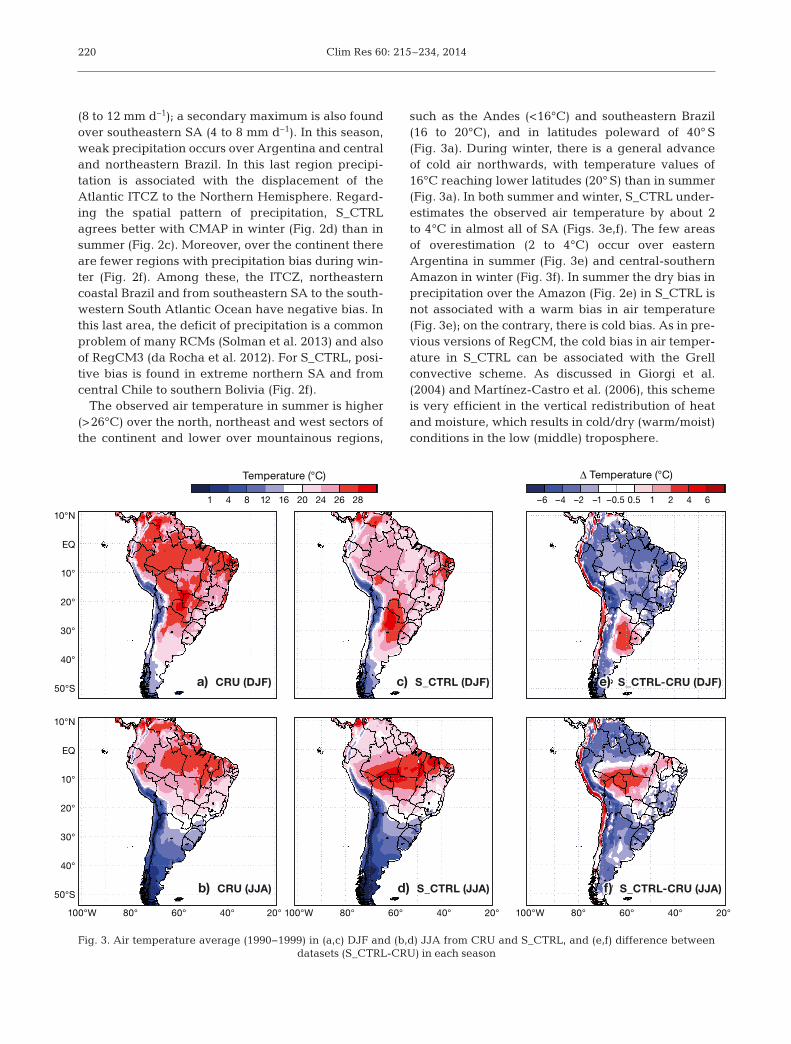
The observed air temperature in summer is higher(>26°C) over the north, northeast and west sectors ofthe continent and lower over mountainous regions,

such as the Andes (<16°C) and southeastern Brazil(16 to 20°C), and in latitudes poleward of 40° S(Fig. 3a). During winter, there is a general advanceof cold air northwards, with temperature values of16°C reaching lower latitudes (20° S) than in summer(Fig. 3a). In both summer and winter, S_CTRL under-estimates the observed air temperature by about 2to 4°C in almost all of SA (Figs. 3e,f). The few areasof overestimation (2 to 4°C) occur over easternArgentina in summer (Fig. 3e) and central-southernAmazon in winter (Fig. 3f). In summer the dry bias inprecipitation over the Amazon (Fig. 2e) in S_CTRL isnot associated with a warm bias in air temperature(Fig. 3e); on the contrary, there is cold bias. As in pre-vious versions of RegCM, the cold bias in air temper-ature in S_CTRL can be associated with the Grellconvective scheme. As discussed in Giorgi et al.(2004) and Martínez-Castro et al. (2006), this schemeis very efficient in the vertical redistribution of heatand moisture, which results in cold/dry (warm/moist)conditions in the low (middle) troposphere.

220

a) CRU (DJF) c) S_CTRL (DJF)

d) S_CTRL (JJA)b) CRU (JJA)

e) S_CTRL-CRU (DJF)

f) S_CTRL-CRU (JJA)

50°S

40°

30°

20°

10°

10°N

EQ

50°S

40°

30°

20°

10°

10°N

1 4 8 12 16 20 24 26 28 6421–1–2–4–6 0.5–0.5

EQ

100°W 80° 60° 40° 20° 100°W

Temperature (°C) ∆ Temperature (°C)

80° 60° 40° 20° 100°W 80° 60° 40° 20°

Fig. 3. Air temperature average (1990−1999) in (a,c) DJF and (b,d) JJA from CRU and S_CTRL, and (e,f) difference between datasets (S_CTRL-CRU) in each season

Reboita et al.: Assessment of RegCM4.3 over South America

3.1. Sensitivity to the convective schemes: S_CTRL, S_MIT and S_Tiedtke

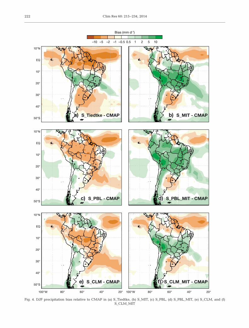
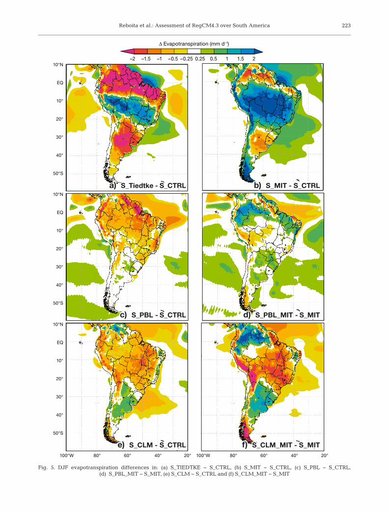
This section compares the performance of 3 of theconvective schemes presented in Table 1 (Mixed1:S_CTRL, Tiedtke: S_Tiedtke, and MIT: S_MIT) in thesimulation of the climatology of precipitation and airtemperature over SA. During austral summer (DJF),S_CTRL overestimates the precipitation over north-ern-central SA, while negative rainfall biases occurover southern Amazon, ITCZ and the oceanic branchof the SACZ (Fig. 2e). On the other hand, a differentspatial pattern of precipitation bias is shown by theS_MIT experiment (Fig. 4b). The use of the MIT con-vective scheme results in very wet conditions overalmost all of Brazil, Bolivia, Peru, Ecuador, and west-ern Argentina. In this experiment, the dry biasesoccur over southeastern SA, eastern Colombia, theextreme north of SA (Guyana and Suriname) and inthe tropical Atlantic ITCZ. This dry condition overthe ITCZ intensifies and extends southward coveringa large part of north-northeastern SA in theS_Tiedtke experiment (Fig. 4a). This simulation alsoin creases the region having negative precipitationbiases in southeastern SA as compared to S_CTRLand S_MIT. A west−east band (from Peru, Bolivia,and crossing from central-western to southeasternBrazil) of positive rainfall biases is also present in theS_Tiedtke (Fig. 4a). The spatial pattern of preci -pitation biases in S_MIT and S_Tiedtke may — atleast in part — be associated with the differences inevapo trans piration. In a large part of the areas whereS_MIT is wetter than CMAP (Fig. 4b) there is alsoa larger evapotranspiration rate than S_CTRL(Fig. 5b). For the whole continental SA we obtain anannual mean evapotranspiration rate of 2.88 and3.61 mm d−1, respectively, in S_CTRL and S_MIT. Weattempt to understand this feature by calculating forthe annual mean the spatial pattern correlationbetween the differences (S_MIT minus S_CTRL) ofevapotranspiration and of some near surface vari-ables only over the continent. The larger evapotran-spiration in S_MIT occurs mainly due to the greaterwater content in the soil layers (upper layer plus rootzone) in S_MIT than in S_CTRL. The correlation ishigh and positive (+0.86) indicating that in regionswith greater (smaller) soil water content the evapo-transpiration is higher (lower).

In S_Tiedtke the areas with large underestimationof rainfall (over northern and southeastern SA inFig. 4a) are the same areas with evapotranspirationrate smaller than in S_CTRL (Fig. 5a). Also in thiscase, there is a high positive spatial pattern correla-

tion (0.93) between the differences (S_Tiedtke minusS_CTRL) of soil moisture and of evapotranspiration,justifying the decrease (increase) of evapotranspira-tion in the areas with lower (higher) total soil watercontent. In addition, in the wetter (S_MIT) and dryer(S_Tiedtke) simulations there is a different partitionof the total rainfall between convective and gridscale. In S_MIT the large evapotranspiration leads toan increase in moist static energy, contributing to theactivation of the convective scheme. Consequently,91% of the total precipitation is convective. The op -posite occurs in S_Tiedtke where the lower evapo-transpiration reduces both the moist static energyand the fraction of the convective rainfall to 61% ofthe total rainfall.

The precipitation biases for the sensitivity experi-ments in austral winter (JJA) are shown in Fig. 6. Inthis season, over continental SA a reduction of theareas presenting precipitation bias is seen in bothS_CTRL (Fig. 2f) and S_MIT (Fig. 6b) as comparedto summer. However, both experiments simulate aband of positive rainfall biases in the southerndomain. Fig. 6a shows that even in winter S_Tiedtkecontinues to present large areas with precipitationunderestimation over the continental SA (most ofnorthern SA, North Atlantic ITCZ, southwesternSouth Atlantic Ocean and the eastern part of north-eastern of Brazil), making it the poorer convectivescheme in winter. The only region where S_Tiedtkesimulates smaller biases than S_CTRL and S_MITis in the oceanic areas at higher latitudes (Figs. 2fand 6a,b).

Figs. 7 and 8 present the air temperature biasesduring austral summer and winter, respectively. Insummer, the large positive differences of S_MIT inrelation to CRU occur over northwestern SA and cen-tral-northern Argentina, while negative differencesare noticed over southeastern Brazil, southern Ar -gen tina and the Andes Mountains (Figs. 7b). The airtemperature bias in S_Tiedtke (Fig. 7a) presents aspatial pattern similar to that of S_MIT (Fig. 7b).However, in S_Tiedtke the more intense warm biascovers practically all of northern-northeastern SA. InS_Tiedtke the warm biases can be due to the under-estimation of precipitation and to greater sensibleheat flux transfer from surface to the low tropospherethan S_CTRL (Fig. not shown). On the other hand,S_CTRL (Fig. 3e) has a cold bias over most of SA,even in areas where a precipitation deficit occurs(Fig. 2e). A common feature in the 3 simulations withdifferent convective schemes (S_CTRL, S_MIT andS_Tiedtke) is the warm bias over southeastern SA,which could be a result of both precipitation under-

221

Clim Res 60: 215–234, 2014222

a) S_Tiedtke - CMAP b) S_MIT - CMAP

d) S_PBL_MIT - CMAPc) S_PBL - CMAP

50°S

40°

30°

20°

10°

10°N

EQ

50°S

40°

30°

20°

10°

10°N

–10 –5 –2 –1 –0.5 0.5 1 2 5 10

EQ

Bias (mm d–1)

f) S_CLM_MIT - CMAPe) S_CLM - CMAP50°S

40°

30°

20°

10°

10°N

EQ

100°W 80° 60° 40° 20° 100°W 80° 60° 40° 20°

Fig. 4. DJF precipitation bias relative to CMAP in (a) S_Tiedtke, (b) S_MIT, (c) S_PBL, (d) S_PBL_MIT, (e) S_CLM, and (f) S_CLM_MIT

Reboita et al.: Assessment of RegCM4.3 over South America 223

a) a) S_T_Tiedtke - S_CTRLS_CTRL b) b) S_MIT - S_MIT - S_CTRLS_CTRL

d) d) S_PBLPBL_MIMIT - S_MITS_MITc) c) S_PBLPBL - S_CTRLS_CTRL

f) f) S_CLM_MIT - S_MITS_CLM_MIT - S_MITe) e) S_CLM - S_CLM - S_CTRLS_CTRL

a) S_Tiedtke - S_CTRL b) S_MIT - S_CTRL

d) S_PBL_MIT - S_MITc) S_PBL - S_CTRL

50°S

40°

30°

20°

10°

10°N

EQ

50°S

40°

30°

20°

10°

10°N

–2 –1.5 –1 –0.5 –0.25 0.50.25 1 1.5 2

EQ

∆ Evapotranspiration (mm d–1)

f) S_CLM_MIT - S_MITe) S_CLM - S_CTRL

50°S

40°

30°

20°

10°

10°N

EQ

100°W 80° 60° 40° 20° 100°W 80° 60° 40° 20°

Fig. 5. DJF evapotranspiration differences in: (a) S_TIEDTKE − S_CTRL, (b) S_MIT − S_CTRL, (c) S_PBL − S_CTRL, (d) S_PBL_MIT − S_MIT, (e) S_CLM − S_CTRL and (f) S_CLM_MIT − S_MIT

Clim Res 60: 215–234, 2014224

a) a) S_T_Tiedtke - CMCMAP b) b) S_MIT - CMAPS_MIT - CMAP

d) d) S_PBLPBL_MIMIT - CMCMAPc) c) S_PBLPBL - CMCMAP

f) f) S_CLM_MIT - CMAPS_CLM_MIT - CMAPe) e) S_CLM - CMAPS_CLM - CMAP

a) S_Tiedtke - CMAP b) S_MIT - CMAP

d) S_PBL_MIT - CMAPc) S_PBL - CMAP

50°S

40°

30°

20°

10°

10°N

EQ

50°S

40°

30°

20°

10°

10°N

–10 –5 –2 –1 –0.5 0.5 1 2 5 10

EQ

Bias (mm d–1)

f) S_CLM_MIT - CMAPe) S_CLM - CMAP50°S

40°

30°

20°

10°

10°N

EQ

100°W 80° 60° 40° 20° 100°W 80° 60° 40° 20°

Fig. 6. Similar to Fig. 4 but for JJA precipitation bias

Reboita et al.: Assessment of RegCM4.3 over South America 225

a) a) S_T_Tiedtke - CRUCRU b) b) S_MIT - CRUS_MIT - CRU

d) d) S_PBLPBL_MIMIT - CRUCRUc) c) S_PBLPBL - CRUCRU

f) f) S_CLM_MIT - CRUS_CLM_MIT - CRUe) e) S_CLM - CRUS_CLM - CRU

a) S_Tiedtke - CRU b) S_MIT - CRU

d) S_PBL_MIT - CRUc) S_PBL - CRU

50°S

40°

30°

20°

10°

10°N

EQ

50°S

40°

30°

20°

10°

10°N

–6 –4 –2 –1 –0.5 0.5 1 2 4 6

EQ

Bias (°C)

f) S_CLM_MIT - CRUe) S_CLM - CRU50°S

40°

30°

20°

10°

10°N

EQ

100°W 80° 60° 40° 20° 100°W 80° 60° 40° 20°

Fig. 7. DJF air temperature bias relative to CRU in (a) S_Tiedtke, (b) S_MIT, (c) S_PBL, (d) S_PBL_MIT, (e) S_CLM, and (f) S_CLM_MIT

Clim Res 60: 215–234, 2014226

a) a) S_T_Tiedtke - CRUCRU b) b) S_MIT - CRUS_MIT - CRU

d) d) S_PBLPBL_MIMIT - CRUCRUc) c) S_PBLPBL - CRUCRU

f) f) S_CLM_MIT - CRUS_CLM_MIT - CRUe) e) S_CLM - CRUS_CLM - CRU

a) S_Tiedtke - CRU b) S_MIT - CRU

d) S_PBL_MIT - CRUc) S_PBL - CRU

50°S

40°

30°

20°

10°

10°N

EQ

50°S

40°

30°

20°

10°

10°N

–6 –4 –2 –1 –0.5 0.5 1 2 4 6

EQ

Bias (°C)

f) S_CLM_MIT - CRUe) S_CLM - CRU50°S

40°

30°

20°

10°

10°N

EQ

100°W 80° 60° 40° 20° 100°W 80° 60° 40° 20°

Fig. 8. Similar to Fig. 7 but for JJA air temperature bias (°C)

Reboita et al.: Assessment of RegCM4.3 over South America

estimation (Figs. 2e and 4a,b) and the PBL scheme(see Section 3.2).

In winter, S_CTRL simulates a warm bias over thesouthern Amazon and the Andes Mountains and asin summer, a cold bias is seen in the other sectors ofSA (Fig. 3f). On other hand, in S_Tiedtke (Fig. 8a)and S_MIT (Fig. 8b) the air temperature simulationerrors have a different spatial pattern. In these exper-iments there are warm biases over the Amazon andvicinity and cold biases over eastern Brazil andextreme southern Argentina.

3.2. Sensitivity to the PBL schemes: S_CTRL, S_PBL and S_PBL_MIT

In this section we discuss the impact of 2 differentPBL schemes, Holtslag (S_CTRL) and UW-PBL(S_PBL), upon the simulated climatology. In addition,we investigate whether the association of the MITscheme with UW-PBL (S_PBL_MIT) might reduce theexcessive positive precipitation bias of the S_MITexperiment during austral summer (Fig. 4b).

Comparing the S_CTRL (Fig. 2e) and S_PBL(Fig. 4c) precipitation biases we can see that in sum-mer over the SACZ (continental and oceanicbranches) and ITCZ regions the UW-PBL schemecontributes to drier conditions in S_PBL than Holtslagin S_CTRL. A large underestimation of rainfall is alsosimulated during winter over northwestern SA andthe ITCZ, due to the influence of the UW-PBL scheme(Fig. 6c). The increase of dry bias in S_PBL is mainlyrelated to the reduction in the evapotranspiration ratecompared with S_CTRL (Fig. 5c). Considering thecontinental SA, the annual mean evapotranspirationrates are 2.35 and 2.88 mm d−1, respectively, in S_PBLand S_CTRL. For lower evapo transpiration in S_PBL,the differences (S_PBL minus S_CTRL) of soil mois-ture and of evapotranspiration also present a highpositive spatial pattern correlation (+0.85). As thecorrelation is positive we may interpret that the areaswith less (more) soil water content are also regionswith less (more) evapotranspiration in S_PBL com-pared with S_CTRL. A second feature is the increaseof surface drag stress in the same areas with lessevapotranspiration, which is ex plained by spatial pattern correlation of −0.77 be tween the differences(S_PBL minus S_CTRL) in evapotranspiration and insurface drag stress. Compared with S_CTRL, in theS_PBL the lowering of the PBL height is not directlyrelated to the increase of evapotranspiration, sincethe differences (S_PBL minus S_CTRL) present weakspatial correlation of only −0.21. In general, regions

with dry bias in S_PBL (Figs. 4c and 6c) become wetwhen the MIT scheme is used together with UW-PBLscheme (Figs. 4d and 6d). This last combination of parameterizations (S_PBL_MIT) contributes to in-creasing the evapotranspiration in some parts ofSA compared with the S_MIT (Fig. 5d) and S_PBL(Fig. not shown) and consequently yield more precip-itation. In S_MIT_PBL the regions with greater (less)evapotranspiration are also positively (negatively)correlated with regions with more (less) soil watercontent (correlation of 0.84) and surface drag stress(correlation −0.80). However, in the S_MIT_PBL, thenegative correlation between regions with lower(higher) PBL height and higher (lower) evapotranspi-ration is greater (−0.64) than for S_PBL (−0.21). Thiscould permit the development of clouds with lowerbase in S_MIT_PBL than in S_PBL, explaining atleast in part the large amount of precipitation inS_MIT_PBL. In this experiment the large part (87%)of total rainfall results from the con vection schemes;this result was also obtained for S_MIT (91%).

For the air temperature, in both summer and winter, compared to CRU the configuration S_PBL(Figs. 7c and 8c) produces a cold bias over almost allof SA, even in the regions with large precipitationunderestimation. In general, the values and spatialpattern of the temperature biases from S_PBL resem-ble that of S_CTRL (Figs. 3e,f), suggesting that theGrell convective scheme dominates over the UW-PBL scheme to produce the cold bias. When S_MIT(Figs. 7b and 8b) and S_PBL_MIT (Figs. 7d and 8d)simulations are compared, the UW-PBL scheme contributes to the reduction of the warm bias of theHoltslag scheme (S_MIT) over northwestern andsoutheastern SA. In this last area, independent ofcon vective scheme, UW-PBL reduces the excessivewarm bias of Holtslag in summer by means of de -creasing the sensible heat fluxes (Figs. not shown).Güttler et al. (2013) used the RegCM4.2 (with BATSand MIT schemes) to evaluate the sensitivity to theHoltslag and UW-PBL schemes over Europe. In thisanalysis they also obtained a reduction of the warmbias with UW-PBL. These authors also suggest thatthe smaller entrainment of potentially warm freetropo spheric air into the boundary layer in UW-PBLcan contribute to decreasing the warm bias.

3.3. Sensitivity to the surface schemes: S_CTRL, S_CLM and S_CLM_MIT

As shown in Table 1, we analyzed the influence ofland surface schemes by changing the BATS to the

227

Clim Res 60: 215–234, 2014

CLM in the S_CLM experiment. Besides this, we car-ried out another simulation using the MIT convectivescheme together with the CLM (S_CLM_MIT).

In the austral summer, by comparing S_CLM withCMAP (Fig. 4e) we can see the underestimation ofprecipitation over the SACZ (continental and oceanicbranches) and ITCZ regions. The spatial pattern ofthis bias differs from that of S_CTRL (which uses theBATS scheme), which has a smaller dry bias in theseoceanic regions and the continent (over southernAmazon, Fig. 2e). On the other hand, the coupling ofCLM with the MIT scheme (Fig. 4f) reduces the sig-nificant overestimate of precipitation in tropical andsubtropical SA (from 5° S to 25° S) and also reducesthe dry bias over southeastern SA present in S_MIT(Fig. 4b). For winter, S_CLM (Fig. 6e) simulates moreareas with negative precipitation bias (northwesternSA, southern Brazil and the adjacent South AtlanticOcean) than S_CTRL (Fig. 2f). In addition, duringwinter S_CLM_MIT (Fig. 6f) presents smaller precip-itation biases than S_MIT (Fig. 6b). This occurs forthe positive and negative rainfall biases, respec-tively, over northwestern SA and southern Brazil.Therefore, in both summer and winter, the combina-tion of CLM with the MIT scheme (S_CLM_MIT) con-tributes to a decrease in wet bias when the combina-tion of the BATS and MIT schemes is used. Thisimprovement in the precipitation simulated byS_CLM_MIT is associated with CLM, which contri -butes to the reduction in the excessive evapotranspi-ration rate simulated by S_MIT (Fig. 5b,f). This factwas also documented by Steiner et al. (2009) andDiro et al. (2012). According to Steiner et al. (2009),soil moisture at the surface is underestimated byCLM compared to BATS, and since the evaporationfrom bare soil is the main contributor to eva po trans -piration in CLM it decreases the latent heat fluxesand precipitation. As a result of the drier soil layersand reduced latent heating, sensible heat fluxes aregenerally higher in CLM.

The coupling of CLM and the MIT scheme inS_CLM_MIT also helps to reduce the temperatureerrors over a large part of SA during the summer(Fig. 7f). The warm biases over northwestern andsoutheastern SA are smaller in S_CLM_MIT than inS_MIT (Fig. 7b). Moreover, S_CLM_MIT presents astrong improvement in the simulated air temperaturecompared to S_CTRL (Fig. 3e) and S_CLM (Fig. 7e),which simulate a cold bias over a large part of SA.Although S_CLM_MIT overestimates the precipita-tion over central-western SA (Fig. 4f), it does not pro-duce a cold bias. This fact can be associated in partwith the influence of the convective scheme. In

S_CTRL (Fig. 3e) and S_CLM (Fig. 7e), which use theGrell scheme over the continent, the underestimationof air temperature is a common feature in both. Asdiscussed, the Grell convective scheme is very effi-cient in the vertical redistribution of heat and mois-ture, explaining in part its near-surface cold bias(Giorgi et al. 2004, Martínez-Castro et al. 2006). Con-sidering all simulations in this study (Fig. 7), thesmallest warm bias over northeastern Argentina issimulated by S_CLM (Fig. 7e).

In winter, S_CTRL (Fig. 3f) and S_CLM (Fig. 8e)show a similar spatial pattern in the bias, i.e. they arewarmer than CRU over the southern Amazon andcolder in other areas. As in summer, the temperaturebias over Amazon is smaller in S_CLM_MIT (Fig. 8f)than in the other simulations. Overall, considering allsimulations and all SA, the air temperature in winteris slightly better simulated by S_CLM_MIT. The nextsection shows that there is a better surface energypartitioning in S_CLM_MIT, which contributes to theimprovement of the simulated air temperature.

3.4. Annual cycle: precipitation and air temperature

The analyses of Sections 3.1, 3.2 and 3.3 suggestthat for the whole of SA the configurations of S_CTRLand S_CLM_MIT are better for the simulation of theprecipitation and air temperature, respectively. How-ever, sometimes these configurations may not beappropriate to the specific regions. Thus, we evalu-ated the performance of the simulations over 5 conti-nental subdomains (indicated in Fig. 1) over theannual cycle by means of statistical indices (bias, SDand Pearson correlation coefficient) applied to theDJF and JJA seasons. The SD was used as a measureof the interannual variability, with high (low) valuesindicating greater (weaker) interannual variability.

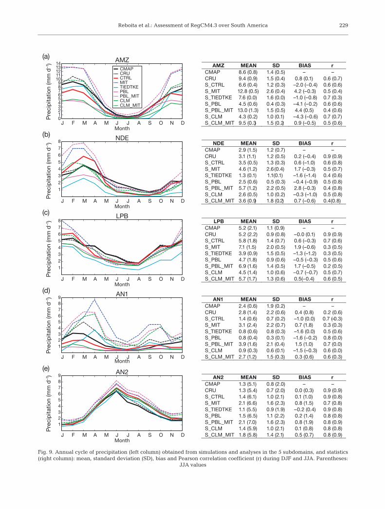
In Fig. 9a, CMAP shows the wet season in theAmazon subdomain (AMZ) occurring from Octoberto March and is associated with the SAM (Vera et al.2006, Marengo et al. 2012), while the dry season lastsfrom April to September. In general, the phase of theannual cycle of precipitation is simulated by all ex -periments. However, in terms of intensity, S_CTRLpresents smaller biases for precipitation from June toNovember and S_CLM_MIT from December toMarch (Fig. 9a). Since DJF is the peak of the AMZrainy season, we will discuss the statistical analysisfor this season.

In DJF, compared with CMAP (Fig. 9a) the MITscheme (S_PBL_MIT and S_MIT) tends to produces

228

Reboita et al.: Assessment of RegCM4.3 over South America 229

(a)AMZ MEAN SD BIAS r

CMAP 8.6 (0.8) 1.4 (0.5) – –CRU 9.4 (0.9) 1.5 (0.4) 0.8 (0.1) 0.6 (0.7)S_CTRL 6.6 (0.4) 1.2 (0.3) –2.0 (–0.4) 0.6 (0.6)S_MIT 12.8 (0.5) 2.6 (0.4) 4.2 (–0.3) 0.5 (0.4)S_TIEDTKE 7.6 (0.0) 1.6 (0.0) –1.0 (–0.8) 0.7 (0.3)S_PBL 4.5 (0.6) 0.4 (0.3) –4.1 (–0.2) 0.6 (0.6)S_PBL_MIT 13.0 (1.3) 1.5 (0.5) 4.4 (0.5) 0.4 (0.6)S_CLM 4.3 (0.2) 1.0 (0.1) –4.3 (–0.6) 0.7 (0.7)S_CLM_MIT 9.5 (0.3) 1.5 (0.2) 0.9 (–0.5) 0.5 (0.6)

(b)NDE MEAN SD BIAS r

CMAP 2.9 (1.5) 1.2 (0.7) – –CRU 3.1 (1.1) 1.2 (0.5) 0.2 (–0.4) 0.9 (0.9)S_CTRL 3.5 (0.5) 1.3 (0.3) 0.6 (–1.0) 0.6 (0.8)S_MIT 4.6 (1.2) 2.6 (0.4) 1.7 (–0.3) 0.5 (0.7)S_TIEDTKE 1.3 (0.1) 1.1(0.1) –1.6 (–1.4) 0.4 (0.6)S_PBL 2.5 (0.6) 0.5 (0.3) –0.4 (–0.9) 0.5 (0.8)S_PBL_MIT 5.7 (1.2) 2.2 (0.5) 2.8 (–0.3) 0.4 (0.8)S_CLM 2.6 (0.5) 1.0 (0.2) –0.3 (–1.0) 0.5 (0.8)S_CLM_MIT 3.6 (0.9) 1.8 (0.2) 0.7 (–0.6) 0.4(0.8)

(c)LPB MEAN SD BIAS r

CMAP 5.2 (2.1) 1.1 (0.9) – –CRU 5.2 (2.2) 0.9 (0.8) –0.0 (0.1) 0.9 (0.9)S_CTRL 5.8 (1.8) 1.4 (0.7) 0.6 (–0.3) 0.7 (0.6)S_MIT 7.1 (1.5) 2.0 (0.5) 1.9 (–0.6) 0.3 (0.5)S_TIEDTKE 3.9 (0.9) 1.5 (0.5) –1.3 (–1.2) 0.3 (0.5)S_PBL 4.7 (1.8) 0.9 (0.6) –0.5 (–0.3) 0.5 (0.6)S_PBL_MIT 6.9 (1.6) 1.4 (0.5) 1.7 (–0.5) 0.2 (0.5)S_CLM 4.5 (1.4) 1.0 (0.6) –0.7 (–0.7) 0.5 (0.7)S_CLM_MIT 5.7 (1.7) 1.3 (0.6) 0.5(–0.4) 0.6 (0.5)

(d)AN1 MEAN SD BIAS r

CMAP 2.4 (0.6) 1.9 (0.2) – –CRU 2.8 (1.4) 2.2 (0.6) 0.4 (0.8) 0.2 (0.6)S_CTRL 1.4 (0.6) 0.7 (0.2) –1.0 (0.0) 0.7 (–0.3)S_MIT 3.1 (2.4) 2.2 (0.7) 0.7 (1.8) 0.3 (0.3)S_TIEDTKE 0.8 (0.6) 0.8 (0.3) –1.6 (0.0) 0.5 (0.6)S_PBL 0.8 (0.4) 0.3 (0.1) –1.6 (–0.2) 0.8 (0.0)S_PBL_MIT 3.9 (1.6) 2.1 (0.4) 1.5 (1.0) 0.7 (0.0)S_CLM 0.9 (0.3) 0.6 (0.1) –1.5 (–0.3) 0.6 (0.0)S_CLM_MIT 2.7 (1.2) 1.5 (0.3) 0.3 (0.6) 0.6 (0.3)

(e)AN2 MEAN SD BIAS r

CMAP 1.3 (5.1) 0.8 (2.0) – –CRU 1.3 (5.4) 0.7 (2.0) 0.0 (0.3) 0.9 (0.9)S_CTRL 1.4 (6.1) 1.0 (2.1) 0.1 (1.0) 0.9 (0.8)S_MIT 2.1 (6.6) 1.6 (2.3) 0.8 (1.5) 0.7 (0.8)S_TIEDTKE 1.1 (5.5) 0.9 (1.9) –0.2 (0.4) 0.9 (0.8)S_PBL 1.5 (6.5) 1.1 (2.2) 0.2 (1.4) 0.8 (0.8)S_PBL_MIT 2.1 (7.0) 1.6 (2.3) 0.8 (1.9) 0.8 (0.9)S_CLM 1.4 (5.9) 1.0 (2.1) 0.1 (0.8) 0.8 (0.8)S_CLM_MIT 1.8 (5.8) 1.4 (2.1) 0.5 (0.7) 0.8 (0.9)

J F M A M J J A S O N D0123456789

1011121314

Month

Pre

cip

itatio

n (m

m d

–1) AMZ

J F M A M J J A S O N D

1

2

3

4

5

6

7

8

Month

Pre

cip

itatio

n (m

m d

–1)

NDE

J F M A M J J A S O N D

1

2

3

4

5

6

7

8

Month

Pre

cip

itatio

n (m

m d

–1)

Pre

cip

itatio

n (m

m d

–1)

Pre

cip

itatio

n (m

m d

–1)

LPB

J F M A M J J A S O N D

123456789

Month

AN1

J F M A M J J A S O N D

123456789

Month

AN2

CMAPCRUCTRLMITTIEDTKEPBLPBL_MITCLMCLM_MIT

Fig. 9. Annual cycle of precipitation (left column) obtained from simulations and analyses in the 5 subdomains, and statistics(right column): mean, standard deviation (SD), bias and Pearson correlation coefficient (r) during DJF and JJA. Parentheses:

JJA values

Clim Res 60: 215–234, 2014230

higher positive rainfall biases in AMZ, except whenassociated with the CLM scheme (S_CLM_MIT). Thelarge underestimates of precipitation occur in theS_PBL and S_CLM experiments. In terms of the SD(Fig. 9), overall the simulated values are near those ofCMAP and CRU, except for S_MIT and S_PBL. Com-pared with CMAP/CRU, higher (lower) than ob servedinterannual variability of precipitation is simulatedby S_MIT (S_PBL). Considering all experiments,S_CLM_MIT and S_PBL_MIT have values close tothe CMAP/CRU, i.e. show considerable ability in sim-ulating the observed interannual variability of rainfall.

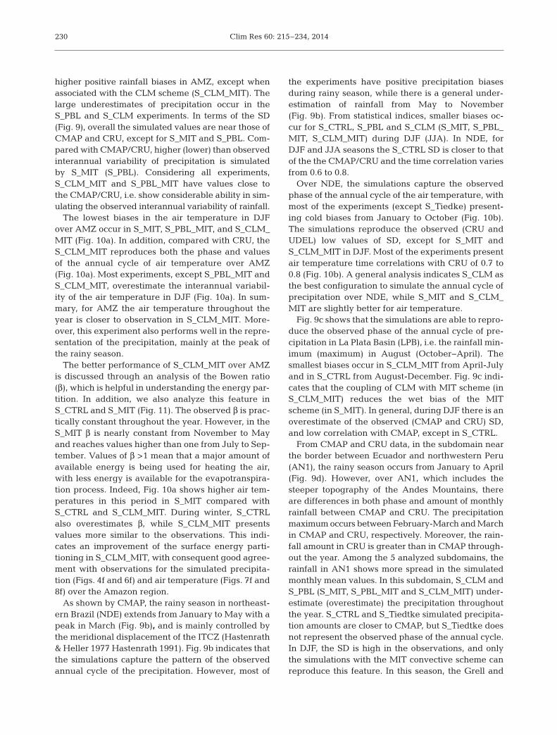
The lowest biases in the air temperature in DJFover AMZ occur in S_MIT, S_PBL_MIT, and S_CLM_MIT (Fig. 10a). In addition, compared with CRU, theS_CLM_MIT reproduces both the phase and valuesof the annual cycle of air temperature over AMZ(Fig. 10a). Most experiments, except S_PBL_MIT andS_CLM_MIT, overestimate the interan nual variabil-ity of the air temperature in DJF (Fig. 10a). In sum-mary, for AMZ the air temperature throughout theyear is closer to observation in S_CLM_MIT. More-over, this experiment also performs well in the repre-sentation of the precipitation, mainly at the peak ofthe rainy season.

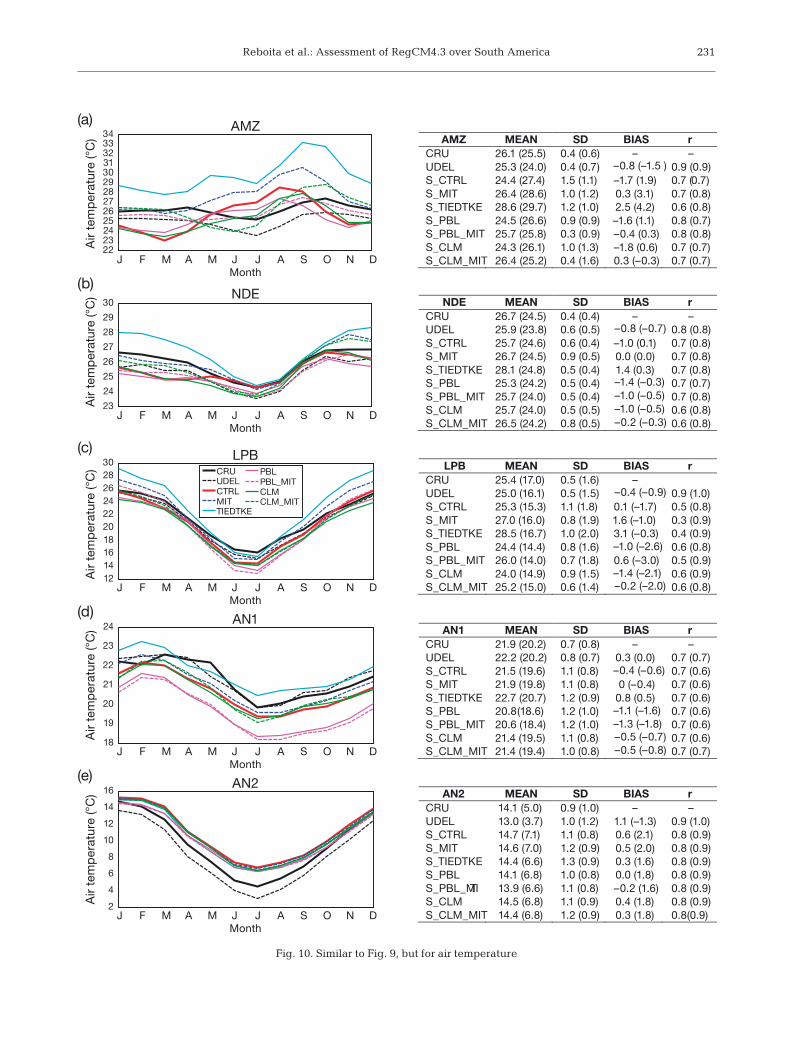
The better performance of S_CLM_MIT over AMZis discussed through an analysis of the Bowen ratio(β), which is helpful in understanding the energy par-tition. In addition, we also analyze this feature inS_CTRL and S_MIT (Fig. 11). The observed β is prac-tically constant throughout the year. However, in theS_MIT β is nearly constant from November to Mayand reaches values higher than one from July to Sep-tember. Values of β >1 mean that a major amount ofavailable energy is being used for heating the air,with less energy is available for the evapotranspira-tion process. Indeed, Fig. 10a shows higher air tem-peratures in this period in S_MIT compared withS_CTRL and S_CLM_MIT. During winter, S_CTRLalso overestimates β, while S_CLM_MIT presentsvalues more similar to the observations. This indi-cates an improvement of the surface energy parti-tioning in S_CLM_MIT, with consequent good agree-ment with observations for the simulated precipita-tion (Figs. 4f and 6f) and air temperature (Figs. 7f and8f) over the Amazon region.

As shown by CMAP, the rainy season in northeast-ern Brazil (NDE) extends from January to May with apeak in March (Fig. 9b), and is mainly controlled bythe meridional displacement of the ITCZ (Hastenrath& Heller 1977 Hastenrath 1991). Fig. 9b indicates thatthe simulations capture the pattern of the observedannual cycle of the precipitation. However, most of

the experiments have positive precipitation biasesduring rainy season, while there is a general under-estimation of rainfall from May to November(Fig. 9b). From statistical indices, smaller biases oc -cur for S_CTRL, S_PBL and S_CLM (S_MIT, S_PBL_MIT, S_CLM_MIT) during DJF (JJA). In NDE, forDJF and JJA seasons the S_CTRL SD is closer to thatof the the CMAP/CRU and the time correlation variesfrom 0.6 to 0.8.

Over NDE, the simulations capture the observedphase of the annual cycle of the air temperature, withmost of the experiments (except S_Tiedke) present-ing cold biases from January to October (Fig. 10b).The simulations reproduce the observed (CRU andUDEL) low values of SD, except for S_MIT andS_CLM_MIT in DJF. Most of the experiments presentair temperature time correlations with CRU of 0.7 to0.8 (Fig. 10b). A general analysis indicates S_CLM asthe best configuration to simulate the annual cycle ofprecipitation over NDE, while S_MIT and S_CLM_MIT are slightly better for air temperature.

Fig. 9c shows that the simulations are able to repro-duce the observed phase of the annual cycle of pre-cipitation in La Plata Basin (LPB), i.e. the rainfall min-imum (maximum) in August (October−April). Thesmallest biases occur in S_CLM_MIT from April-Julyand in S_CTRL from August-December. Fig. 9c indi-cates that the coupling of CLM with MIT scheme (inS_CLM_MIT) reduces the wet bias of the MITscheme (in S_MIT). In general, during DJF there is anoverestimate of the observed (CMAP and CRU) SD,and low correlation with CMAP, except in S_CTRL.

From CMAP and CRU data, in the subdomain nearthe border between Ecuador and northwestern Peru(AN1), the rainy season occurs from January to April(Fig. 9d). However, over AN1, which includes thesteeper topography of the Andes Mountains, thereare differences in both phase and amount of monthlyrainfall between CMAP and CRU. The precipitationmaximum occurs between February-March and Marchin CMAP and CRU, respectively. Moreover, the rain-fall amount in CRU is greater than in CMAP through-out the year. Among the 5 analyzed subdomains, therainfall in AN1 shows more spread in the simulatedmonthly mean values. In this subdomain, S_CLM andS_PBL (S_MIT, S_PBL_MIT and S_CLM_MIT) under-estimate (overestimate) the precipitation through outthe year. S_CTRL and S_Tiedtke simulated precipita-tion amounts are closer to CMAP, but S_Tiedtke doesnot represent the observed phase of the annual cycle.In DJF, the SD is high in the observations, and onlythe simulations with the MIT convective scheme canreproduce this feature. In this season, the Grell and

Reboita et al.: Assessment of RegCM4.3 over South America 231

AMZ MEAN SD BIAS rCRU 26.1 (25.5) 0.4 (0.6) – –UDEL 25.3 (24.0) 0.4 (0.7) –0.8 (–1.5 ) 0.9 (0.9)S_CTRL 24.4 (27.4) 1.5 (1.1) –1.7 (1.9) 0.7 (0.7)S_MIT 26.4 (28.6) 1.0 (1.2) 0.3 (3.1) 0.7 (0.8)S_TIEDTKE 28.6 (29.7) 1.2 (1.0) 2.5 (4.2) 0.6 (0.8)S_PBL 24.5 (26.6) 0.9 (0.9) –1.6 (1.1) 0.8 (0.7)S_PBL_MIT 25.7 (25.8) 0.3 (0.9) –0.4 (0.3) 0.8 (0.8)S_CLM 24.3 (26.1) 1.0 (1.3) –1.8 (0.6) 0.7 (0.7)S_CLM_MIT 26.4 (25.2) 0.4 (1.6) 0.3 (–0.3) 0.7 (0.7)

NDE MEAN SD BIAS rCRU 26.7 (24.5) 0.4 (0.4) – –UDEL 25.9 (23.8) 0.6 (0.5) –0.8 (–0.7) 0.8 (0.8)S_CTRL 25.7 (24.6) 0.6 (0.4) –1.0 (0.1) 0.7 (0.8)S_MIT 26.7 (24.5) 0.9 (0.5) 0.0 (0.0) 0.7 (0.8)S_TIEDTKE 28.1 (24.8) 0.5 (0.4) 1.4 (0.3) 0.7 (0.8)S_PBL 25.3 (24.2) 0.5 (0.4) –1.4 (–0.3) 0.7 (0.7)S_PBL_MIT 25.7 (24.0) 0.5 (0.4) –1.0 (–0.5) 0.7 (0.8)S_CLM 25.7 (24.0) 0.5 (0.5) –1.0 (–0.5) 0.6 (0.8)S_CLM_MIT 26.5 (24.2) 0.8 (0.5) –0.2 (–0.3) 0.6 (0.8)

LPB MEAN SD BIAS rCRU 25.4 (17.0) 0.5 (1.6) –UDEL 25.0 (16.1) 0.5 (1.5) –0.4 (–0.9) 0.9 (1.0)S_CTRL 25.3 (15.3) 1.1 (1.8) 0.1 (–1.7) 0.5 (0.8)S_MIT 27.0 (16.0) 0.8 (1.9) 1.6 (–1.0) 0.3 (0.9)S_TIEDTKE 28.5 (16.7) 1.0 (2.0) 3.1 (–0.3) 0.4 (0.9)S_PBL 24.4 (14.4) 0.8 (1.6) –1.0 (–2.6) 0.6 (0.8)S_PBL_MIT 26.0 (14.0) 0.7 (1.8) 0.6 (–3.0) 0.5 (0.9)S_CLM 24.0 (14.9) 0.9 (1.5) –1.4 (–2.1) 0.6 (0.9)S_CLM_MIT 25.2 (15.0) 0.6 (1.4) –0.2 (–2.0) 0.6 (0.8)

AN1 MEAN SD BIAS rCRU 21.9 (20.2) 0.7 (0.8) – –UDEL 22.2 (20.2) 0.8 (0.7) 0.3 (0.0) 0.7 (0.7)S_CTRL 21.5 (19.6) 1.1 (0.8) –0.4 (–0.6) 0.7 (0.6)S_MIT 21.9 (19.8) 1.1 (0.8) 0 (–0.4) 0.7 (0.6)S_TIEDTKE 22.7 (20.7) 1.2 (0.9) 0.8 (0.5) 0.7 (0.6)S_PBL 20.8 (18.6) 1.2 (1.0) –1.1 (–1.6) 0.7 (0.6)S_PBL_MIT 20.6 (18.4) 1.2 (1.0) –1.3 (–1.8) 0.7 (0.6)S_CLM 21.4 (19.5) 1.1 (0.8) –0.5 (–0.7) 0.7 (0.6)S_CLM_MIT 21.4 (19.4) 1.0 (0.8) –0.5 (–0.8) 0.7 (0.7)

AN2 MEAN SD BIAS rCRU 14.1 (5.0) 0.9 (1.0) – –UDEL 13.0 (3.7) 1.0 (1.2) 1.1 (–1.3) 0.9 (1.0)S_CTRL 14.7 (7.1) 1.1 (0.8) 0.6 (2.1) 0.8 (0.9)S_MIT 14.6 (7.0) 1.2 (0.9) 0.5 (2.0) 0.8 (0.9)S_TIEDTKE 14.4 (6.6) 1.3 (0.9) 0.3 (1.6) 0.8 (0.9)S_PBL 14.1 (6.8) 1.0 (0.8) 0.0 (1.8) 0.8 (0.9)S_PBL_MIT 13.9 (6.6) 1.1 (0.8) –0.2 (1.6) 0.8 (0.9)S_CLM 14.5 (6.8) 1.1 (0.9) 0.4 (1.8) 0.8 (0.9)S_CLM_MIT 14.4 (6.8) 1.2 (0.9) 0.3 (1.8) 0.8(0.9)

22232425262728293031323334

23

24

25

26

27

28

29

30

12141618202224262830

18

19

20

21

22

23

24

2

4

6

8

10

12

14

16

CRUUDELCTRLMITTIEDTKE

PBLPBL_MITCLMCLM_MIT

(a)

(b)

(c)

(d)

(e)

J F M A M J J A S O N DMonth

Air

tem

per

atur

e (°

C)

AMZ

J F M A M J J A S O N DMonth

Air

tem

per

atur

e (°

C) NDE

J F M A M J J A S O N DMonth

Air

tem

per

atur

e (°

C)

Air

tem

per

atur

e (°

C)

Air

tem

per

atur

e (°

C)

LPB

J F M A M J J A S O N DMonth

AN1

J F M A M J J A S O N DMonth

AN2

Fig. 10. Similar to Fig. 9, but for air temperature

Clim Res 60: 215–234, 2014232

Tiedtke convective schemes simulate lower interan-nual variability than that observed.

In southern Chile (AN2), precipitation is condi-tioned by the meridional migration of the SouthPacific Subtropical Anticyclone (Aceituno 1980),which moves northward in JJA, favoring precipita-tion. As shown by CMAP (Fig. 9e), JJA is the rainyseason over AN2, as presented also by Reboita et al.(2010c) and Rojas (2006). The simulations reproducethe observed phase of the annual cycle of precipita-tion but, in general, overestimate it from June toNovember (Fig. 9e). The lowest rainfall bias occurswith S_Tiedtke and the highest biases in S_MIT andS_PBL_MIT. AN2 is the subdomain where the simu-lations present the highest correlations with CMAP,in DJF as well as JJA. In addition, in JJA the simu-lated SDs are closer to CMAP than during DJF. Theseindices indicate that the simulations better representthe observed interannual variability in AN2 duringthe rainy season.

The phases of the annual cycle of air temperaturein LPB, AN1 and AN2 in the simulations are in accordwith the CRU and UDEL data (Figs. 10c−e). Consid-ering DJF, over the LPB (Fig. 10c), S_CTRL andS_CLM_MIT (S_Tiedke) present the lowest (highest)bias in air temperature. For the AN1 subdomain(Fig. 10d), S_PBL and S_PBL_MIT underestimate theair temperature compared to CRU, while other simu-lations are closer to this analysis. The simulationspresent positive bias over AN2 (Fig. 10e) during mostof the year.

4. CONCLUSIONS

This study analyzed the best RegCM4.3 configura-tions for the simulation of the climate of SA. We car-ried out 7 simulations from January 1989 to January2000. The control simulation (S_CTRL) used theMixed1, Holtslag, and BATS schemes for cumulusconvection, PBL and surface interactions, respec-tively. In the other simulations we changed these

schemes using the new options of RegCM4.3, consid-ering 3 groups: sensitivity to convection schemes(Mixed1, MIT and Tiedtke), sensitivity to planetaryboundary layer (PBL) schemes (Holtslag and UW-PBL) and sensitivity to surface schemes (BATS andCLM). From these 3 groups, S_CTRL simulated thespatial pattern of the precipitation and its intensitywith remarkable agreement with CMAP. However,the air temperature presents good agreement withobservations when the MIT convective scheme isused (S_MIT, S_PBL_MIT, S_CLM_MIT). Therefore,we can conclude that the MIT convective scheme isimportant to climate studies that focus mainly on SAair temperature, while the Mixed1 scheme is recom-mended for precipitation (except in the Amazonregion where S_CLM_MIT is better).

Simulations using the MIT convective scheme pre-sented higher wet bias compared to CMAP than thatwith Mixed1 (Grell over the continent). The reason isthat the MIT scheme overestimates evapotranspira-tion. Another interesting result is when the PBLscheme is changed from Holtslag to UW-PBL, the dryand wet biases, respectively, remain for the experi-ments with Mixed1 (S_PBL) and with MIT (S_PBL_MIT). Therefore, the convective scheme has greatercontrol over precipitation than the PBL scheme. WhenCLM is coupled in the simulations, it contributes todecreases in evapotranspiration. Thus, (1) the dry biasincreases in the experiment with Mixed1 (S_CLM)when it is compared to the experiment with Mixed1and BATS (S_CTRL); and (2) the wet bias decreases inthe experiment S_CLM_MIT (CLM with MIT) when itis compared to the experiment S_MIT (BATS withMIT). The combination of CLM and MIT produces thebest simulation of air temperature over SA.

In the subdomain analysis, RegCM4.3 is able to sim-ulate the phase and intensity of the precipitation andthe annual cycles of air temperature in most of thesubdomains. Some results need to be highlighted: Al-though the Tiedtke scheme does not have a realisticperformance over a large part of SA, it presentedgood agreement with observations in the simulationof the annual cycle of precipitation over southernChile. S_CLM has a more realistic representation ofthe rainy season over northeastern Brazil. On theother hand, S_CLM_MIT is the only simulation thatproduces an annual cycle of air temperature similar tothat observed over Amazon. This last result can be as-sociated with the better energy partition (latent andsensible heat fluxes) in the S_CLM_MIT simulation,which presents a Bowen Ratio lower <1, which is com-parable to the observations. Over La Plata basin andnorthern Peru, S_CTRL simulates both precipitation

Fig. 11. Bowen Ratio (β) for S_CTRL, S_MIT andS_CLM_MIT experiments and observations in Amazon (see

Section 2.2 for more details)

Reboita et al.: Assessment of RegCM4.3 over South America

and air temperature well, providing good agreementwith the observations.

Based on the whole analysis, we recommend theconfigurations of S_CTRL (with these schemes:Mixed1-cumulus convection, Holtslag-PBL, BATS-surface interactions), and S_CLM_MIT (with theseschemes: MIT-cumulus convection, Holtslag-PBL,CLM-surface interactions) as the best configurationsof RegCM4.3 for conducting the simulations of theCORDEX project over SA.

Acknowledgements. We thank the RegCM team (mainly Filippo Giorgi and Graziano Giuliani) and ECMWF, CRU andCMAP for the datasets. Thanks also to the CAPES/ PROCAD-179/2007, CAPES-PROEX, and CNPq (307202/ 2011-12) forpartial financial support and to the 3 anonymous reviewerswhose suggestions helped us to improve the manuscript.

LITERATURE CITED

Aceituno P (1980) Relation entre la posicion del anticiclonsubtropical y la precipitación en Chile. Project ReportE.551.791, University of Chile, Santiago

Anthes RA (1977) A cumulus parameterization scheme uti-lizing a one-dimensional cloud model. Mon Weather Rev105: 270−286

Anthes RA, Hsie EY, Kuo YH (1987) Description of the PennState/NCAR mesoscale model version 4 (MM4). TechNote TN-282+STR, National Center for AtmosphericResearch, Boulder, CO

Bowen IS (1926) The ratio of heat losses by conduction andevaporation from any surface. Phys Rev 27: 779−789

Bretherton CS, McCaa JR, Grenier H (2004) A new parame-terization for shallow cumulus convection and its appli-cation to marine subtropical cloud-topped boundary lay-ers. I. Description and 1D Results. Mon Weather Rev 132: 864−882

Brohan P, Kennedy JJ, Harris I, Tett SFB, Jones PD (2006)Uncertainty estimates in regional and global observedtemperature changes: a new dataset from 1850. J Geo-phys Res 111: D12106, doi: 10.1029/2005JD006548

Chou SC, Nunes AMB, Cavalcanti IAF (2000) Extendedrange forecasts over South America using the regionaleta model. J Geophys Res 105: 10147−10160

da Rocha RP, Morales CA, Cuadra SV, Ambrizzi T (2009)Precipitation diurnal cycle and summer climatologyassess ment over South America: an evaluation ofRegional Climate Model Version 3 simulations. J Geo-phys Res 114: D10108, doi: 10.1029/2008JD010212

da Rocha RP, Cuadra SV, Reboita MS, Kruger LF, AmbrizziT, Krusche N (2012) Effects of RegCM3 parameteriza-tions on simulated rainy season over South America.Clim Res 52: 253−265

Dee DP, Uppala SM, Simmons AJ, Berrisford P, and others(2011) The ERA-Interim reanalysis: configuration andperformance of the data assimilation system. QJR Mete-orol Soc 137: 553−597

Dickinson RE, Errico RM, Giorgi F, Bates GT (1989) Aregional climate model for the western United States.Clim Change 15: 383−422

Dickinson RE, Henderson-Sellers A, Kennedy PJ (1993) Bio-sphere−Atmosphere Transfer Scheme (BATS) version 1E

as coupled to the NCAR community climate model. Tech.Note NCAR/TN-3871STR, National Center for Atmos-pheric Research, Boulder, CO

Diro GT, Rauscher SA, Giorgi F, Tompkins AM (2012) Sensi-tivity of seasonal climate and diurnal precipitation overCentral America to land and sea surface schemes inRegCM4. Clim Res 52: 31−48

Emanuel KA (1991) A scheme for representing cumulus con-vection in large-scale models. J Atmos Sci 48: 2313−2335

Emanuel KA, Zivkovic-Rothman M (1999) Development andevaluation of a convection scheme for use in climatemodels. J Atmos Sci 56: 1766−1782

Fernandez JPR, Franchito SH, Rao VB (2006a) Simulation ofsummer circulation over South America by 2 regional cli-mate models. I. Mean climatology. Theor Appl Climatol86: 247−260

Fernandez JPR, Franchito SH, Rao VB (2006b) Simulation ofthe summer circulation over South America by tworegional climate models. II. A comparison between 1997/1998 El Niño and 1998/1999 La Niña events. Theor ApplClimatol 86: 261−270.

Giorgi F, Marinucci MR (1991) Validation of a regionalatmospheric model over Europe: sensitivity of wintertimeand summertime simulations to selected physics parame-terizations and lower boundary conditions. QJR Meteo-rol Soc 117: 1171−1206

Giorgi F, Marinucci MR, Bates G (1993a) Development of asecond generation regional climate model (RegCM2). I.Boundary layer and radiative transfer processes. MonWeather Rev 121: 2794−2813

Giorgi F, Marinucci MR, Bates G, De Canio G (1993b) Devel-opment of a second generation regional climate model(RegCM2). II. Convective processes and assimilation oflateral boundary conditions. Mon Weather Rev 121: 2814−2832

Giorgi F, Bi X, Pal JS (2004) Mean, interannual variabilityand trends in a regional climate experiment over Europe.I. Present day climate (1960−1990). Clim Dyn 22: 733−756

Giorgi F, Jones C, Asrar G (2009) Addressing climate infor-mation needs at the regional level: the CORDEX frame-work. World Meterol Organ Bull 58: 175−183

Giorgi F, Coppola E, Solmon F, Mariotti L and others (2012)RegCM4: model description and preliminary tests overmultiple CORDEX domains. Clim Res 52: 7−29.

Grell GA (1993) Prognostic evaluation of assumptions usedby cumulus parameterizations. Mon Weather Rev 121: 764−787

Grenier H, Bretherton CS (2001) A moist PBL parameteriza-tion for large scale models and its application to subtrop-ical cloud-topped marine boundary layers. Mon WeatherRev 129: 357−377

Güttler I, Brankovic C, O’Brien TA, Coppola E, Grisogono B,Giorgi F (2013) Sensitivity of the regional climate modelRegCM4.2 to planetary boundary layer parameteriza-tion. Clim Dyn, doi: 10. 1007/s00382-013-2003-6

Hastenrath S (1991) Climate Dynamics of the Tropics.Kluwer Academic Publishers, Dordrecht

Hastenrath S, Heller L (1977) Dynamics of climatic hazardsin northeast Brazil. QJR Meteorol Soc 103: 77−92

Holtslag A, de Bruijn E, Pan HL (1990) A high resolution airmass transformation model for short-range weather fore-casting. Mon Weather Rev 118: 1561−1575

Krüger LF, da Rocha RP, Reboita MS, Ambrizzi T (2012)RegCM3 nested in HadAM3 scenarios A2 and B2: pro-jected changes in extratropical cyclogenesis, tempera-ture and precipitation over the South Atlantic Ocean.Clim Change 113: 599−621.

233

Clim Res 60: 215–234, 2014

Legates DR, Willmott CJ (1990) Mean seasonal and spatialvariability in global surface air temperature. Theor ApplClimatol 41: 11−21

Loveland TR, Reed BC, Brown JF, Ohlen DO, Zhu Z, Yang L,Merchant JW (2000) Development of a global land covercharacteristics database and IGBP DISCover from 1 kmAVHRR data. Int J Remote Sens 21: 1303 − 1365

Marengo JA, Liebmann B, Grimm AM, Misra V and others(2012) Recent developments on the South Americanmonsoon system. Int J Climatol 32: 1−21

Marengo JA, Ambrizzi T, da Rocha RP, Alves LM and others(2010) Future change of climate in South America in thelate twenty-first century: intercomparison of scenariosfrom three regional climate models. Clim Dyn 35: 1073−1097

Martínez-Castro D, da Rocha RP, Bezanilla A, Alvarez L,Fernández JPR, Silva Y, Arritt R (2006) Sensitivity studiesof the RegCM-3 simulation of summer precipitation, tem-perature and local wind field in the Caribbean Region.Theor Appl Climatol 86: 5−22

Menéndez CG, Saulo AC, Li ZX (2001) Simulation of SouthAmerican wintertime climate with a nesting system.Clim Dyn 17: 219−231

Misra V, Dirmeyer PA, Kirtman BP, Juang HMH, KanamitsuM (2002) Regional simulation of interannual variabilityover South America. J Geophys Res 107 (D20), doi: 10.1029/ 2001JD900216

Negrón Juárez RI, Hodnett MG, Fu R, Goulden ML, vonRandow C (2007) Control of dry season evapotranspira-tion over Amazonian forest as inferred from observationsat a southern Amazon forest site. J Clim 20: 2827−2839

Nicolini M, Salio P, Katzfey JJ, McGregor JL, Saulo AC(2002) January and July regional climate simulation overSouth American. J Geophys Res 107: 4637, doi: 10. 1029/2001 JD000736

Nobre PA, Moura D, Sun L (2001) Dynamical downscaling ofseasonal climate prediction over Nordeste Brazil withECHAM3 and NCEP’s Regional Spectral Models at IRI.Bull Am Meteorol Soc 82: 2787−2796

Nunes AMB, Roads JO (2005) Improving regional modelsimulations with precipitation assimilation. Earth Inter-act 9: 1−44

Nuñez MN, Solman SA, Carbré MF (2009) Regional climatechange experiments over southern South America. II.Climate change scenarios in the late twenty-first century.Clim Dyn 32: 1081−1095

O’Brien TAO, Chuang PY, Sloan LC, Faloona IC, Rossiter DL(2012) Coupling a new turbulence parametrization toRegCM adds realistic stratocumulus clouds. GeosciModel Dev 5: 989−1008

Oleson KW, Dai Y, Bonan G, Bosilovich M and others (2004)Technical description of the community land model.Tech Note NCAR/ TN-461+STR, National Center forAtmospheric Research NCAR, Boulder, CO

Oleson KW, Niu GY, Yang ZL, Lawrence DM and others(2008) Improvements to the community land model andtheir impact on the hydrologic cycle. J Geophys Res 113: G01021, doi: 10.1029/2007JG000563

Pal JS, Giorgi F, Bi X, Elguindi N, and others (2007) Regionalclimate modeling for the developing world: the ICTPRegCM3 and RegCNET. Bull Am Meteorol Soc 88: 1395−1409

Rauscher SA, Seth A, Liebmann B, Qian JH, Camargo SJ(2007) Regional climate model−simulated timing andcharacter of seasonal rains in South America. MonWeather Rev 135: 2642−2657

Reboita MS, da Rocha RP, Ambrizzi T, Shigetoshi S (2010a)

South Atlantic Ocean cyclogenesis climatology simu-lated by regional climate model (RegCM3). Clim Dyn 35: 1331−1347

Reboita MS, da Rocha RP, Ambrizzi T, Caetano E (2010b) Anassessment of the latent and sensible heat flux on thesimulated regional climate over Southwestern SouthAtlantic Ocean. Clim Dyn 34: 873−889

Reboita MS, Gan MA, da Rocha RP, Ambrizzi T (2010c)Regimes de precipitação na América do Sul: uma revisãobibliográfica. Rev Bras Med 25: 185−204

Reboita MS, da Rocha RP, Krüger LF (2013) Climate fore-cast to southern Minas Gerais state. Scientific Report473153/2010-6, CNPq, Brasília

Reynolds RW, Rayner NA, Smith TM, Stokes DC, Wang W(2002) An improved in situ and satellite SST analysis forclimate. J Clim 15: 1609−1625

Rocha HR, Manzi AO, Cabral OM, Miller SD, and others(2009) Patterns of water and heat flux across a biome gra-dient from tropical forest to savanna in Brazil. J GeophysRes 114: G00B12, doi: 10.1029/2007JG000640

Rojas M (2006) Multiply nested regional climate simulationfor southern South America: sensitivity to model resolu-tion. Mon Weather Rev 134: 2208−2223

Sellers PJ, Dickinson RE, Randall DA, Betts AK and others(1997) Modeling the exchanges of energy, water, andcarbon between continents and the atmosphere. Science275: 502−509

Sen OL, Wang Y, Wang B (2004) Impact of Indochina defor-estation on the East-Asian summer monsoon. J Clim 17: 1366−1380

Seth A, Rojas M (2003) Simulation and sensitivity in a nestedmodeling system for tropical South America. I. Reanaly-ses boundary forcing. J Clim 16: 2437−2453

Seth A, Rauscher SA, Camargo SJ, Qian JH, Pal JS (2007)RegCM3 regional climatologies for South America usingreanalysis and ECHAM global model driving fields. ClimDyn 28: 461−480

Solman SA, Sanchez E, Samuelsson P, da Rocha RP and oth-ers (2013) Evaluation of an ensemble of regional climatemodel simulations over South America driven by theERA-Interim reanalysis: model performance and uncer-tainties. Clim Dyn 41: 1139−1157

Steiner AL, Pal JS, Giorgi F, Dickinson RE, Chameides WL(2005) Coupling of the common land model (CLM0) to aregional climate model (RegCM). Theor Appl Climatol82: 225−243

Steiner AL, Pal JS, Rauscher SA, Bell JL and others (2009)Land surface coupling in regional climate simulations ofthe West Africa monsoon. Clim Dyn 33(6): 869-892,

Tawfik AB, Steiner AL (2011) The role of soil ice inland−atmosphere coupling over the United States: a soilmoisture precipitation winter feedback mechanism.J Geophys Res 116: D02113, doi: 10.1029/2010JD014333

Tiedtke M (1989) A comprehensive mass-flux scheme forcumulus parameterization in large-scale models. MonWeather Rev 117: 1779−1800

Vera C, Higgins W, Amador J, Ambrizzi T and otherss (2006)Toward a unified view of the American monsoon sys-tems. J Clim 19: 4977−5000

Xie P, Arkin PA (1997) Global precipitation: a 17-yearmonthly analysis based on gauge observations, satelliteestimates, and numerical model outputs. Bull Am Meteo-rol Soc 78: 2539−2558

Zeng X, Zhao M, Dickinson RE (1998) Intercomparison ofbulk aerodynamic algorithms for the computation of seasurface fluxes using TOGA COARE and TAO data.J Clim 11: 2628−2644

234

Editorial responsibility: Filippo Giorgi, Trieste, Italy

Submitted: June 5, 2013; Accepted: May 2, 2014Proofs received from author(s): July 17, 2014