ASURVEYOFSPATIALEXTREMES:MEASURINGSPATIAL DEPENDENCE AND ... · ASURVEYOFSPATIALEXTREMES:MEASURINGSPATIAL DEPENDENCE AND MODELING SPATIAL ... lies at the intersection of two branches

REVSTAT – Statistical Journal

Volume 10, Number 1, March 2012, 135–165

A SURVEY OF SPATIAL EXTREMES: MEASURING SPATIAL

DEPENDENCE AND MODELING SPATIAL EFFECTS

Authors: Daniel Cooley

– Department of Statistics, Colorado State University,Fort Collins, CO, USA ([email protected])

Jessi Cisewski

– Department of Statistics and Operations Research,University of North Carolina at Chapel Hill,Chapel Hill, NC, USA ([email protected])

Robert J. Erhardt


Soyoung Jeon


Elizabeth Mannshardt

– Department of Statistics, The Ohio State University,Columbus, OH, USA ([email protected])

Bernard Oguna Omolo

– Division of Mathematics and Computer Science,University of South Carolina – Upstate,Spartanburg, SC, USA ([email protected])

Ying Sun

– Statistical and Applied Mathematical Sciences Institute,Research Triangle Park, NC, USA ([email protected])

Abstract:

• We survey the current practice of analyzing spatial extreme data, which lies at the in-tersection of extreme value theory and geostatistics. Characterizations of multivariatemax-stable distributions typically assume specific univariate marginal distributions,and their statistical applications generally require capturing the tail behavior of themargins and describing the tail dependence among the components. We review currentmethodology for spatial extremes analysis, discuss the extension of the finite-dimen-sional extremes framework to spatial processes, review spatial dependence metricsfor extremes, survey current modeling practice for the task of modeling marginaldistributions, and then examine max-stable process models and copula approachesfor modeling residual spatial dependence after accounting for marginal effects.

Key-Words:

• copula; extremal coefficient; hierarchical model; madogram; max-stable process; multi-

variate extreme value distribution.

AMS Subject Classification:

• 62M30, 62H11, 62H20.

136 D. Cooley et al.

A Survey of Spatial Extremes 137

1. INTRODUCTION

Assessing the behavior of rare events such as the risk of flooding, potential

crop damage from drought, or health effects of potential extreme air pollution

events presents unique statistical challenges, and requires one to characterize the

tail of the distribution of the quantity of interest. Since many quantities such as

rainfall, temperature, or air pollution are measured at specifically-located mon-

itors, spatial modeling is necessary. Applications such as these have motivated

the development of methods and tools for analyzing and characterizing spatial

extreme data. In this paper, we survey the current practice of spatial extremes.

Recently, Davison et al. (2012) review spatial extremes methods via a case study

of extreme precipitation in Switzerland. This survey can be viewed as comple-

mentary to Davison et al. (2012), and we aim to provide an entry point for the

study of spatial extremes.

An analysis of spatial extreme data lies at the intersection of two branches

of statistics: extreme value analysis and geostatistics. Below, we give brief in-

troductions to each field. There are a number of books in each field which give

comprehensive overviews. For extremes, references include de Haan & Ferreira

(2006), Beirlant et al. (2004) and Coles (2001); geostatistics references include

Schabenberger & Gotway (2005), Banerjee et al. (2004) and Cressie (1993). For

many studies, spatial effects are often separated into large scale (i.e., regional)

effects and small scale (i.e., local) effects.

In terms of a statistical model, regional spatial effects are often captured

by characterizing how the marginal distribution varies over a study region. Local

spatial effects are typically described by a dependence structure. Given data,

the distinction between the local and regional effects is likely not obvious, and

one can view the task of separating these two effects as analogous to the task

of decomposing time series data into mean (trend and seasonal effects) and a

stationary noise process described by a covariance structure (Brockwell & Davis,

2002, §1.3.3).

Spatial data are necessarily multivariate as they are recorded at multiple

locations. Throughout, we will assume that we analyze only one quantity (e.g.,

rainfall) at multiple sites, although spatially analyzing multiple quantities is a

possible extension of the work surveyed herein.

Spatial data are often modeled as a realization of a spatial process which is

observed at a finite set of locations. We, too, will consider a spatial process, but

we begin with a review of the theory and statistical practice for finite-dimensional

extremes in order to introduce important concepts.


1.1. Multivariate extremes: theory and practice

We assume that the reader is familiar with univariate extreme value theory

and its statistical application. For background on the univariate case see the

monographs by Coles (2001), Beirlant et al. (2004), and de Haan & Ferreira

(2006).

The notion of max-stability forms the foundation of extreme value theory.

Let Xi = (Xi,1, ..., Xi,d)T, i= 1, ..., n, be an i.i.d. sequence of d-dimensional con-

tinuous random vectors, and letMn=(Mn,1, ...,Mn,d)T=(∨ni=1Xi,1, ...,

∨ni=1Xi,d

)

T

,

where∨

denotes the maximum. Assume there exist normalizing sequences {an}and {bn} such that

Pr

(

Mn− bnan

≤ y)

−→ G(y) , n −→ ∞

where the division is understood to be element-wise and G is non-degenerate.

Then G belongs to the class of multivariate max-stable (equivalently, extreme

value) distributions. We will denote by Y = (Y1, ..., Yd)T a max-stable random

vector; that is, a−1n (Mn−bn) d→ Y . The i.i.d. assumption can be relaxed and the

multivariate max-stable distributions continue to serve as the possible limiting

distributions, if certain mixing conditions are met (Leadbetter et al., 1983).

Unlike in the univariate case, no fully parametric representation exists for

the multivariate max-stable distributions. The univariate marginal distributions

must be univariate max-stable and therefore can be described by the generalized

extreme value (GEV) distribution:

(1.1) Pr(

Yj ≤ y)

= Gj(y) = exp

{

−[

(

1 + ξjy − µjσj

)−1/ξj

+

]}

,

for j = 1, ..., d. Here, µj , σj and ξj are the location, scale and shape parame-

ters for the j th component’s marginal and x+ = max(0, x). Accounting for each

GEV marginal is a nuisance, and representations for multivariate max-stable dis-

tributions generally presuppose that the marginals have a common, convenient

max-stable distribution. Throughout, we will assume Z = (Z1, ..., Zd)T has a

multivariate max-stable distribution with unit-Frechet marginals: Pr(Zj ≤ z) =

exp(−z−1). Then

Pr(Z ≤ z) = G∗(z) = exp{

−V (z)}

,(1.2)

V (z) = d

∫

∆d

d∨

j=1

wjzjH(dw) .(1.3)

Here ∆d ={

w ∈ Rd+ | w1 + ··· + wd = 1

}

is the (d− 1)-dimensional simplex, and

the angular (or spectral) measure H is a probability measure on ∆d, which de-


termines the dependence structure of the random vector. Due to the common

marginals, H obeys the moment conditions∫

∆dwj H(dw) = 1/d for j = 1, ..., d.

There is no loss of generality in assuming the multivariate max-stable dis-

tribution has unit-Frechet margins, as Resnick (1987, Prop. 5.10) states that the

domain-of-attraction condition is preserved under monotone transformations of

the marginal distributions. If a−1n (Mn− bn) d→ Y which does not have unit-

Frechet marginals, from (1.1) one can define marginal transformations

Tj(x) =

(

1 + ξjx− µjσj

)−ξj

, j = 1, ..., d ,

and define

G∗(z1, ..., zd) = G{

T←1 (z1), ..., T←d (zd)

}

,

where T←j is the inverse function of Tj , for j = 1, ..., d. This approach of trans-

forming to convenient marginals is similar to copula approaches, albeit with a

marginal suggested by extreme value theory rather than Uniform [0,1].

The above asymptotic theory suggests the following general statistical

methodology, referred to as the block maxima approach. Choose n to be a fixed

block size which is large enough such that the asymptotic theory holds approxi-

mately, and assume a sequence of i.i.d. Xi, i = 1, ..., nm, are observed, where m

denotes the number of blocks. DefineMk=(∨kni=(k−1)n+1Xi,1, ...,

∨kni=(k−1)n+1Xi,d

)

T

for k = 1, ...,m (note that the dependence on n in the notation Mk has been sup-

pressed), and fit a multivariate max-stable distribution to theMk. It is important

to note that Mk will not appear in the observation record unless the occurrence

times of each element’s block maximum coincide.

Using representation (1.2) to fit a multivariate max-stable distribution re-

quires that the marginals be unit Frechet. Although transforming the marginals

is a simple theoretical procedure, in practice the marginal distributions must be

estimated. Subsequently, utilizing (1.2) to perform a multivariate analysis of ex-

tremes involves two tasks: (1) estimating the marginals, and (2) characterizing

the dependence via a model for V (z) or H(w). Tasks (1) and (2) seem sequential;

however, we note that inference can be performed all-at-once either in the fre-

quentist (Padoan et al., 2010) or Bayesian (Ribatet et al., 2011) settings.

For spatial extremes studies, the aforementioned regional and local spatial

effects each can be associated with one of the above tasks. Most study regions are

large enough that the marginal distribution of the studied quantity will vary over

the region. Thus, in order to transform to a common marginal, one must first

account for how the distribution’s tail varies by location. The local spatial effect

is related to the spatial extent of individual extreme events and the resulting

dependence in the data due to multiple sites being affected by the same event.

In terms of (1.2), this dependence is captured by V (z) or H(w). We will refer to


the dependence remaining after the marginal standardization as ‘residual’ depen-

dence, as Sang & Gelfand (2010) termed the data after marginal transformation as

‘standardized residuals’. There is a useful analogy here drawn from atmospheric

science: these two types of spatial effects can be thought of as corresponding to

‘climate’ and ‘weather’ effects. Climate can be thought of as the distribution of

weather (Guttorp & Xu, 2011), and climate varies with location. Performing the

marginal transformation is akin to standardizing the climate across the study re-

gion. Weather events have a spatial extent which is best captured by a stochastic

representation. For most applications, there is a difference in the scale of these

two spatial effects. Climate varies on a larger (regional) spatial scale, and can

be largely (but often not completely) characterized by covariates such as latitude

and elevation. Weather spatial effects, particularly for extremes, are often more

localized.

Although all data are finite-dimensional, a finite-dimensional framework

can be inadequate for dealing with unobserved locations, and thus most classical

spatial work assumes a stochastic process framework. Let S be a study region,

and let s denote a location in a study region. For spatial applications, most

often s ∈ R2 and we will assume this throughout. We will assume Xi(s) is a

stochastic process, where it may be helpful to think of i as indexing the day of

the observation. A fundamental construct for spatial extremes is the max-stable

process, which is the infinite-dimensional analogue to a max-stable random vector.

If for all s ∈ S there exist normalizing sequences an(s) and bn(s) such that

(1.4) a−1n (s)

{

maxi=1,...,n

Xi(s) − bn(s)}

d−→ Y (s) ,

which has a non-degenerate distribution, then Y (s) is a max-stable process.

When the max-stable process has unit Frechet margins, we will denote it by Z(s).

Given any finite set of locations s1, ..., sd, one can let Xi = (Xi(s1), ..., Xi(sd))T

or Z = (Z(s1), ..., Z(sd))T and return to the finite-dimensional setting.

An alternative approach to analyzing block maxima is to instead select

and analyze a subset of threshold exceedances. Although there has been work

to develop methods for multivariate threshold exceedance data, most spatial ex-

tremes work to date has aimed at developing max-stable models and fitting block-

maximum data. This survey will primarily focus on such work, but we briefly

discuss ongoing work in developing methods for spatial threshold exceedance data

in the discussion in §5.

1.2. Standard geostatistics

LetX(s) be a stochastic process. The field of geostatistics provides a frame-

work for exploring, modeling, and predicting or interpolating X(s). Much of clas-


sical geostatistics tries to characterize X(s) in terms of its mean and covariance

function. One typically thinks of using the mean to represent large scale changes

of X(s) and the covariance function to capture the variability due to small- and

micro-scale stochastic sources (Schabenberger & Gotway, 2005, p. 132).

A basic model can be formulated as

(1.5) X(s) = α(s) + e(s) ,

where α(s) is the (non-random) mean function and e(s) is a zero-mean stochastic

process. Often, a regression relation is assumed for the mean function: α(s) =

W (s)Tβ, where W (s) is a vector of covariate information at location s and β is

a vector of regression coefficients.

The process e tries to account for any behavior not captured by the mean

function α. A simple geostatistical model may assume e(s) is second-order sta-

tionary and isotropic. Stationarity implies that the covariance does not depend

on location, i.e., Cov(e(s), e(s′)) = Cov(e(s+h), e(s′+h)), while isotropy implies

that covariance is a function of distance only, i.e., Cov(e(s), e(s + h)) = C(h),

where h = ‖h‖. At times it is useful to further assume that e(s) is a Gaussian

process, which in turn implies X(s) is a Gaussian process with mean α(s).

The second-order stationary and isotropic random field e is characterized

by its covariance function C(h) or equivalently its semivariogram

γ(h) =1

2Var[

e(s+h) − e(s)]

=1

2E[

{

e(s+h) − e(s)}2]

.

Since the covariance function or semivariogram must satisfy several requirements

to be valid, models for C(h) or γ(h) are generally selected from parametric families

(see Schabenberger & Gotway, 2005, §4.2) known to meet these requirements.

Less restrictive than second-order stationary is intrinsic stationarity, which

implies that a process has stationary increments, i.e., e(s)−e(s+h)d= e(h)−e(0).

An intrinsically stationary process can be viewed as akin to a random walk in time

series, which is stationary after differencing. An intrinsically stationary process

does not have a covariance function C(h) but does have a semivariogram γ(h).

A geostatistical analysis often begins with an exploratory phase where de-

pendence is investigated via an empirical covariogram or semivariogram. As best

as one can, one must first account for large scale effects in the mean as “much

damage can be done by applying semivariogram estimators ... to data from non-

stationary spatial processes” (Schabenberger & Gotway, 2005, p. 135). Assuming

stationarity and isotropy, the traditional sample semivariogram is

(1.6) γ(h) =1

2 |N (h)|∑

(s,s′)∈N (h)

{

e(s) − e(s′)}2,


where N (h) denotes the number of pairs (s, s′) separated by the distance h.

Applying the empirical semivariogram to observations provides insight for semi-

variogram model selection. Having selected a parametric family γφ(h) for the

semivariogram function, one often proceeds to estimate the model parameters

φ and β.

A primary goal of many geostatistics analyses is spatial prediction / inter-

polation employing an estimated semivariogram, which is known as kriging.

The point predictor from kriging corresponds to the best linear unbiased pre-

dictor (or the conditional expectation under a Gaussian assumption) of the value

of X(s0) at unobserved location s0 given observed values X(s1), ..., X(sd).

Prediction uncertainty is typically quantified in terms of mean-square prediction

error.

There is an analogy between the two tasks described in §1.1 and the geo-

statistics model (1.5). If e is stationary and Gaussian, then the marginal distri-

bution can only vary with α(s) which captures the regional spatial effects. After

accounting for regional effects with α, the residual dependence in e is character-

ized by its semivariogram or covariance function.

There are important fundamental differences between geostatistics and spa-

tial extremes. As it is based on first and second moments, geostatistics focuses on

central tendencies, not on the distribution’s tail. The Gaussian framework which

is never far from a traditional geostatistics analysis is incorrect for data that are

maxima, as the Gaussian distribution is not max-stable. Dependence in extremes

is described via the exponent measure function V (z) or angular measure H(w)

which cannot be linked to covariance. Finally, much of classical geostatistics is

applied to situations where one has only one realization of the process X(s),

observed at multiple locations. To perform an extreme value analysis, it is nec-

essary that multiple realizations Xi(s) underlie the subset of extreme data which

are eventually analyzed.

Much of the paper will study max-stable processes, and we need to extend

the notion of stationarity and isotropy to these processes. Stationarity for max-

stable processes is first-order, implying invariance of any finite-dimensional joint

distribution to translation:

Pr(

Y (s1) ≤ y1, ..., Y (sd) ≤ yd

)

= Pr(

Y (s1 +h) ≤ y1, ..., Y (sd +h) ≤ yd

)

.

Isotropy will imply that all bivariate joint distributions are also invariant to ro-

tation:

Pr(

Y (s) ≤ y1, Y (s+h) ≤ y2

)

= Pr(

Y (s) ≤ y1, Y (s+h′) ≤ y2

)

,

if ‖h‖ = ‖h′‖. For simplicity, we will generally assume that a random field is

stationary and isotropic.


The remainder of the paper is structured to follow the order of a possible

spatial extremes analysis. We begin by reviewing tools which measure spatial

dependence in §2. In §3 we survey methods for modeling the marginal tail be-

havior over a study region. In §4, we review two primary methods for model-

ing the residual dependence: max-stable process models and copula approaches.

We conclude with a discussion which mentions work in development, challenges

posed by applications, and open problems.

2. MEASURING SPATIAL DEPENDENCE

To completely characterize the dependence among the components of a

max-stable random vector requires one to specify the angular measure H(w) or

the exponent measure function V (z). Specification of H(w) or V (z) is arduous,

especially as the dimension d grows, and representations are not easily compared.

It is useful to have summary measures of tail dependence, and several metrics

have been developed which aim to summarize the amount of tail dependence in

one number.

A complication arises because tail dependence falls into two distinct cat-

egories: asymptotic dependence and asymptotic independence. Since the cate-

gories are distinct, summary measures for dependence have been developed for

each category. We first focus on metrics for the asymptotic dependence case,

with a particular interest in measuring dependence in terms of spatial distance.

We then explain the notion of asymptotic independence (which does not imply

complete independence) and briefly mention how the amount of dependence in

the asymptotic independence case can be measured.

We note that the metrics all assume at least that random vectors or fields

have a common marginal distribution. Like in geostatistics, one must first try to

account for large-scale marginal effects before using these tools to assess (residual)

dependence.

2.1. Tail dependence metrics for asymptotic dependence

There are many related metrics for quantifying tail dependence when the

random vector exhibits asymptotic dependence. The list includes the metric d of

Davis & Resnick (1989) and the metric χ of Coles et al. (1999). We focus on two

metrics: the extremal coefficient (Smith, 1990; Schlather & Tawn, 2003) which is

readily interpretable and the madogram (Cooley et al., 2006; Naveau et al., 2009)

which has ties to the semivariogram.


2.1.1. Extremal coefficient

Let Y be a d-dimensional max-stable random variable with common mar-

gins. The d-dimensional extremal coefficient θd can be implicitly defined as

Pr(

Y1 ≤ y, ..., Yd ≤ y)

= Pr

(

d∨

j=1

Yj ≤ y

)

= Prθd(

Y1 ≤ y)

,

for any y in the support of Y1. Transforming the marginals of Y to obtain Z,

and due to the homogeneity property of V , we have

(2.1) Pr(

Z1 ≤ z, ..., Zd ≤ z)

= exp{

−z−1V (1, ..., 1)}

⇒ θd = V (1, ..., 1) .

The value θd can be thought of as the effective number of independent random

variables in the d-dimensional random vector. The coefficient takes values be-

tween 1 and d, with a value of 1 corresponding to complete dependence among

the locations, and a value of d corresponding to complete independence. The ex-

tremal coefficient is studied extensively in Schlather & Tawn (2003) and relations

between extremal coefficients of different orders are given in Schlather & Tawn

(2002).

Given replicates of a d-dimensional random vector Z, Smith (1990) and

Coles & Dixon (1999) propose an estimator of the extremal coefficient θd. As Z

has unit Frechet margins, 1/Zj is unit exponential, and 1/∨dj=1 Zj is exponential

with mean 1/θd. Given i.i.d. replicates Zk, k = 1, ...,m, a simple estimator is

(2.2) θd =m

∑mk=1 1

/∨dj=1(zk,j)

,

where zk,j is the j th component of the observation zk.

Although higher-order extremal coefficients are sometimes useful (see

Erhardt & Smith, 2011), θ2 is most widely used as it conveys the amount of

dependence between a pair of components. Bivariate dependence metrics are

especially useful in spatial studies as one generally wants to link the level of de-

pendence to spatial distance. Let Z(s) be a stationary and isotropic max-stable

random field with unit-Frechet margins. It is possible to extend (2.1) to be a

distance-based dependence metric:

θ(h) = Pr(

Z(s) ≤ z, Z(s+h) ≤ z)

.

One could extend (2.2) to construct a distance-based estimator for θ(h); how-

ever, to our knowledge, distance-based dependence summary measures have been

primarily estimated via the madogram (for instance, see the SpatialExtremes

package in R, Ribatet, 2011).


2.1.2. Madogram

The madogram, a first-order semivariogram, has its roots in geostatistics

and its properties were studied by Matheron (1987). Since the madogram requires

the first-moment to be finite which is not always the case in extremes studies,

Cooley et al. (2006) proposed the F-madogram, which first transforms the ran-

dom variable by applying the cdf and is finite for any distribution. If Y (s) is a

stationary and isotropic max-stable process with marginal distribution G, then

the F-madogram is:

(2.3) ν(h) =1

2E

∣

∣

∣G{

Y (s)}

−G{

Y (s+h)}

∣

∣

∣

(for consistency with above, we have used G, rather than F , to denote a max-

stable marginal distribution). The F-madogram’s values range from 0 to 1/6,

which corresponds to complete dependence and independence respectively. The

F-madogram is related to the other extremal dependence metrics, as Cooley et al.

(2006) show that

(2.4) θ(h) =1 + 2 ν(h)

1 − 2 ν(h).

●

●

●

●

●

●

●

●

●

●

●

●

●

●

●

●

●●

●

●

●

●

●

●

●

●

●

●

●

●

●●

●

●

●

●

●

●

●●

●

●

●

●

●

●

●

●

●

●

●

●

●●

●

●

●

●

●

●

●

●

●

●

●

●

●

●

●●

●●

●●

●

●

●

● ●

●

●

●

●●

●

●

●

●

●

●

●

●

●

●

●

●

●

●

●

●

●

●

●

●

●

●

●

●

●

●●

●

●

●

●●

●

●

●●

●

●

●

●

●

●

●

●

●

●

●

●

●

●

●

●

●●

●

●

●

●

●

●

●

●

●

●

●

●

●

●●●

●

●

●

●

●

●●

●●

●●

●

●

●

●

●

●

●

●

●

●

●

●●

●

●

●

●

●

●

●●

●

●

●

●●

●

●

●

●

●

●

●

●

●

●

●

●

●

●

●

●

●

●

●

●

●

●

●

●

●

●

●

●

●

●

●

●

●

●

●

●●

●

●

●

●

●

●

●

●

●

●

●

●

●

●

●

●

●

●

●

●

●

●●●

●

●

●

●

●

●

●

●

●

●

●

●

●

●

●

●

●

●

●

●

●

●

●●

●

●

●

●

●

●

●

●

●

●

●

●

●

●

●

●

●

●

●

●

●

●

●

●

●

●

●●

●

●

●

●

●

●

●

●

●

●●

●

●

●

●

●

●

●

●

●

●

●

●

●

●

●

●

●

●

●

●

●

●●

●●

●

●

●

●

●

●●

●

●

●

●

●

●

●

●

●

●

●●

●

●

●

●

●

●

●

●

●●

●

●

●

●

●

●

●

●

●

●

●

●

●

●

●

●

●

●●

●●

●

●

●

●

●

●●

●

●

●

●●

●

●

●

● ●

●

●

●

●

●

●

●

● ●

●

●

●

●

●

●

●

●

●

●

●

●

●

●

●● ●

●

●

●

●

●

●

●

●

●

●

●

●

●

●●

●

●

●

●

●

●

● ●●

●

●

●

●

●

●

●

●

●

●

●

●

●

●

●●

●

●

●

●

●

●●● ●

●●

●

●●

●

●

●

●

●

●

●

●

●●

●

●

●●

●

●

●

●

●

●

●

●

●

●

●

●

●

●

●

●

●

●

●

●

●

●

●

●

●

●

●

●

●

●

●

●

●

●

●

●

● ●

●

●

●

●

●

●

●●

●

●

●

●

●

●

●

●

●

●

●

●

●

●

●

●

●

●

●

●

●

●

●

●

●

●

●

●

●

●

●

●

●

●

●●

● ●

●

●

●

●

●

●

●

●

●

●

●

●

●

●

●

●

●

●

●

●

●●

●

●

●

●

●

●

●

●●

●

●

●

●

●

●

●

●

●

●●

●

●

●

●

●

●

●

●

●

●

●

●

●

●

●

●

●

●

●

●●

●

●●

●

●

●

●

●

●

●

●●

● ●

●

●

●

●

●●

● ●

●

●

●

●

●

●

●

●

●●

●

●

●

●

●

●

●

●

●

●

●

●●

● ●●

●

●

● ●

●

●

●

●

●

●

●

●

●●

●

●

●

●

●

●

●

●

●

●

●

●

●

●

●●

●

●

●

●

●

●

●

●

●

●

●

●

●

●

●

●

●

●

●

●

●●

●

●

●

●

●

● ●

● ●

●

●

●

●

●

●●

●

●

●

●

●

●

●

●●

●

●

●

●

●

●

●

0 2 4 6 8 10 12

1.0

1.2

1.4

1.6

1.8

2.0

h

θ(h

)

●

●

●

●

●

●

●

●

●

●

●

●

●

●

●

●

●●

●

●

●

●

●

●

●

●

●

●

●

●

●●

●

●

●

●

●

●

●●

●

●

●

●

●

●

●

●

●

●

●

●

●●

●

●

●

●

●

●

●

●

●

●

●

●

●

●

●●

●●

●●

●

●

●

●●

●

●

●

●

●

●

●

●

●

●

●

●

●

●

●

●

●

●

●

●

●

●

●

●

●

●

●

●

●

●

●●

●

●

●

●

●

●

●

●●

●

●

●

●

●

●

●

●

●

●

●

●

●

●

●

●

●●

●

●

●

●

●

●

●

●

●

●

●

●

●

●●●

●

●

●

●

●

●●

●●

●●

●

●

●

●

●

●

●

●

●

●

●

●

●

●

●

●

●

●

●

●●

●

●

●

●●

●

●

●

●

●

●

●

●

●

●

●

●

●

●

●

●

●

●

●

●

●

●

●

●

●

●

●

●

●

●

●

●

●

●

●

●●

●

●

●

●

●

●

●

●

●

●

●

●

●

●

●

●

●

●

●

●

●

●●●

●

●

●

●

●

●

●

●

●

●

●

●

●

●

●

●

●

●

●

●

●

●

●●

●

●

●

●

●

●

●

●

●

●

●

●

●

●

●

●

●

●

●

●

●

●

●

●

●

●

●

●

●

●

●

●

●

●

●

●

●

●●

●

●

●

●

●

●

●

●

●

●

●

●

●

●

●

●

●

●

●

●

●

●

●

●●

●

●

●

●

●

●●

●

●

●

●

●

●

●

●

●

●

●●

●

●

●

●

●

●

●

●

●●

●

●

●

●

●

●

●

●

●

●

●

●

●

●

●

●

●

●●

●●

●

●

●

●

●

●●

●

●

●

●

●

●

●

●

● ●

●

●

●

●

●

●

●

●●

●

●

●

●

●

●

●

●

●

●

●

●

●

●

●● ●

●

●

●

●

●

●

●

●

●

●

●

●

●

●●

●

●

●

●

●

●

●●●

●

●

●

●

●

●

●

●

●

●

●

●

●

●

●●

●

●

●

●

●

●

●● ●

●●

●

●●

●

●

●

●

●

●

●

●

●●

●

●

●●

●

●

●

●

●

●

●

●

●

●

●

●

●

●

●

●

●

●

●

●

●

●

●

●

●

●

●

●

●

●

●

●

●

●

●

●

● ●

●

●

●

●

●

●

●●

●

●

●

●

●

●

●

●

●

●

●

●

●

●

●

●

●

●

●

●

●

●

●

●

●

●

●

●

●

●

●

●

●

●

●●

● ●

●

●

●

●

●

●

●

●

●

●

●

●

●

●

●

●

●

●

●

●

●●

●

●

●

●

●

●

●

●

●

●

●

●

●

●

●

●

●

●

●●

●

●

●

●

●

●

●

●

●

●

●

●

●

●

●

●

●

●

●

●●

●

●●

●

●

●

●

●

●

●

●●

● ●

●

●

●

●

●

●

● ●

●

●

●

●

●

●

●

●

●●

●

●

●

●

●

●

●

●

●

●

●

●●

● ●●

●

●

● ●

●

●

●

●

●

●

●

●

●●

●

●

●

●

●

●

●

●

●

●

●

●

●

●

●●

●

●

●

●

●

●

●

●

●

●

●

●

●

●

●

●

●

●

●

●

●

●

●

●

●

●

●

● ●

● ●

●

●

●

●

●

●●

●

●

●

●

●

●

●

●●

●

●

●

●

●

●

●

0 2 4 6 8 10 12

0.0

20

.06

0.1

00

.14

h

νF(h

)

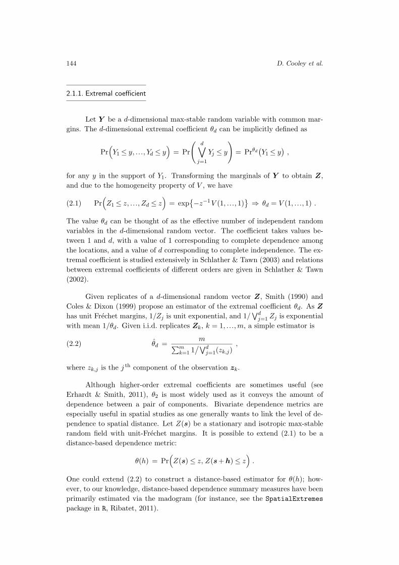
Figure 1: Extremal coefficient (left panel) and the F-Madogram (rightpanel) with unit Gumbel margins for the Schlather model withWhittle–Matern correlation functions. The red lines are thetheoretical extremal coefficient and F-madogram, gray pointsare pairwise estimates, and black crosses are binned estimates.


An advantage of the F-madogram is that its definition (2.3) suggests an

estimator. Let yk(s), k = 1, ...,m, be i.i.d. replicates of a max-stable process

with marginal distribution G which is observed at a finite set of locations. Then

the sample F-madogram is given by

(2.5) ν(h) =1

m

m∑

k=1

1

2 |N (h)|∑

(s,s′)∈N (h)

∣

∣G{

yk(s)}

−G{

yk(s′)}∣

∣ ,

analogous to the semivariogram estimator (1.6). An estimator θ(h) can be ob-

tained via a plug-in estimator from (2.4). Equation (2.5) assumes that the

marginal distribution G is known. Naveau et al. (2009) discuss estimation of

the madogram when the marginal distribution is not known and further define

the λ-madogram, which is related to the Pickands’ dependence function and which

extends the notion of the madogram to completely describe the bivariate depen-

dence structure.

2.2. Asymptotic independence

Two componentsX1 andX2 from a random vectorX with common margin-

als are asymptotically independent if

(2.6) limx→x∗

Pr(

X2 > x | X1 > x)

= 0 ,

where x∗ is the upper endpoint of the common marginal distribution. The com-

ponents are asymptotically dependent if the limit in (2.6) is a non-zero constant.

If asymptotically independent, then (X1, X2) lie in the domain of attraction of

max-stable (Y1, Y2), whose angular measure H(w) has a mass of 1/2 at w = (0, 1)

and at w = (1, 0), and 0 elsewhere. That is, the bivariate angular measure has

mass only on the axes. The extremal coefficient of (Y1, Y2) is 2, correspondingly.

Asymptotic independence does not imply (complete) independence and, in

fact, can mask relevant dependencies. The canonical example is that if (X1, X2)

is standard bivariate normal with fixed correlation ρ < 1, then it can be shown

(Sibuya, 1960) that the variables are asymptotically independent. Summarizing

tail dependence with the extremal coefficient or madogram, or modeling tail de-

pendence via H(w) or V (z), will ignore any dependence in an asymptotically

independent couple.

Ledford and Tawn (1996) identified the problems arising with the existing

modeling methodology in the case of asymptotic independence and proposed a

new parameter η, the coefficient of tail dependence. If (Z1, Z2) has unit Frechet


marginals, Ledford and Tawn (1996) assume a joint survival function F satisfying

F (z, z) = Pr(

Z1 > z, Z2 > z)

∼ L(z) z−1/η , z → ∞ ,

where L is a slowly varying function (L(tz)/L(z) → 1 as z → ∞) and η ∈ (0, 1].1

The coefficient of tail dependence η is used to quantify the tail dependence in the

asymptotic independent setting; η = 1 implies asymptotic dependence and η < 1

measures the degree of dependence under asymptotic independence. Ledford and

Tawn (1996) spawned much subsequent work including other estimators for η

(Draisma et al., 2004; Peng, 1999), development of other dependence measures

in the asymptotic independence setting (Coles et al., 1999), and development of

models in the case of asymptotic independence (Ledford & Tawn, 1997; Heffernan

& Tawn, 2004; Ramos & Ledford, 2009).

Models for and measures of tail dependence for spatial extremes have thus

far been limited to the asymptotically dependent case. However, an understand-

ing of the concept of asymptotic independence is essential to fully understanding

the limitations of summary dependence metrics such as θ(h) and for understand-

ing the models for residual dependence presented in §4.

3. CAPTURING SPATIAL STRUCTURE IN MARGINAL

BEHAVIOR

The representation of multivariate max-stable distributions (1.2) as well

as the spatial dependence models in §§4.1, 4.2 presuppose that the univariate

marginal distributions are known and common at all locations in the study region.

In most applications, the study regions are large enough that the assumption of a

common marginal distribution is unrealistic and the marginal distribution is not

known. Therefore, it becomes essential to model the marginal distribution at all

locations within the study region.

A simplistic approach would be to individually estimate the marginal dis-

tributions at each location. This approach has been used in (non-spatial) multi-

variate applications (e.g., Heffernan & Tawn, 2004; Cooley et al., 2010). Such an

approach is less-than-ideal for spatial applications for a number of reasons. First,

a goal of many spatial projects is to make inference at locations where there are

no data, i.e., to perform spatial interpolation. Constructing unconnected models

at each location does not allow one to readily interpolate. Second, there is a

desire to borrow strength across locations when estimating marginal parameters.

Many spatial data have a temporal record of several decades. Such a data record

1We use F to denote the cdf as Ledford and Tawn (1996) do not require that (Z1, Z2) bemax-stable.


is more-than-enough to pin down the central tendencies of the marginal distribu-

tion, but large uncertainties remain about tail quantities. It is well-documented

that tail quantities, and in particular point estimates for the tail index ξ, can

vary wildly over the spatial region when estimated individually (e.g., Cooley &

Sain (2010)). Methods which borrow strength across locations ‘trade space for

time’ and help to reduce uncertainties.

Below we briefly detail several methods used to capture spatial structure

when describing the tail of the marginal distribution before focusing on the recent

approach of hierarchical modeling.

3.1. Methods for marginal parameter estimation

As mentioned in §1.2, regression approaches are frequently used to model

the mean process α(s) of a geostatistical model. Similarly, regression approaches

have been used to model the parameters of the extreme value distributions. When

modeling annual maximum precipitation in the southeast United States, Padoan

et al. (2010) select a model in which the location parameter µ(s) and scale param-

eter σ(s) are linear functions of latitude and elevation, and the shape parameter

ξ(s) is constant over the study region. Padoan et al. (2010) go on to model the

residual dependence via a max-stable process (see §4.1). Mannshardt-Shamseldin

et al. (2010) use a spatial regression approach which downscales extreme pre-

cipitation as generated by climate models to that observed at weather stations.

Generally, one wishes to employ covariates which are known at all locations s ∈ S(both observed and unobserved), and often spatial coordinates are the only such

covariates. In geostatistics, regression models on spatial coordinates are known

as trend surface models (Schabenberger & Gotway, 2005, §5.3.1). However simple

regression models on available covariates are sometimes unable to fully capture

complex spatial behavior, and Ribatet et al. (2011) found this to be the case

in a study of extreme precipitation in Switzerland. Regional frequency analy-

sis (RFA) (Hosking & Wallis, 1997) is a term for a statistical procedure which

explicitly borrows strength across locations and which in turn characterizes the

spatial nature of the tail of the marginal distribution. RFA has a long history in

hydrology and traces its roots to the index flood procedure of Dalrymple (1960).

RFA is a multi-step procedure which pools data over predefined subregions of Sdetermined to be ‘homogeneous’. Hosking & Wallis (1997) advocate an esti-

mation method based on L-moments for RFA. A recent effort to update the

precipitation-frequency atlases for the United States (Bonnin et al., 2004a,b) em-

ploys an L-moment-based RFA coupled with an interpolation method based on

the PRISM method (Daly et al., 1994, 2002). A possible disadvantage of RFA is

that it does not construct an explicit spatial model for the marginal parameters.

To our knowledge, no RFA-based work has tried to account for residual depen-

dence in the data after accounting for marginal effects.


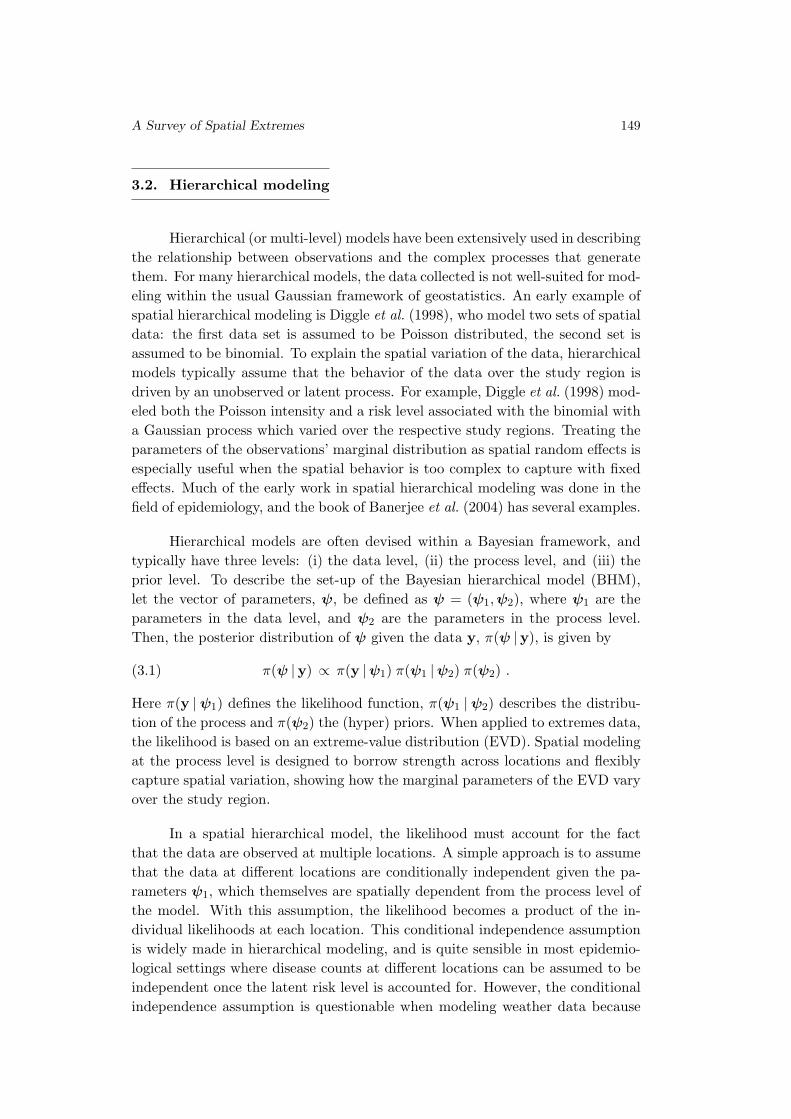
3.2. Hierarchical modeling

Hierarchical (or multi-level) models have been extensively used in describing

the relationship between observations and the complex processes that generate

them. For many hierarchical models, the data collected is not well-suited for mod-

eling within the usual Gaussian framework of geostatistics. An early example of

spatial hierarchical modeling is Diggle et al. (1998), who model two sets of spatial

data: the first data set is assumed to be Poisson distributed, the second set is

assumed to be binomial. To explain the spatial variation of the data, hierarchical

models typically assume that the behavior of the data over the study region is

driven by an unobserved or latent process. For example, Diggle et al. (1998) mod-

eled both the Poisson intensity and a risk level associated with the binomial with

a Gaussian process which varied over the respective study regions. Treating the

parameters of the observations’ marginal distribution as spatial random effects is

especially useful when the spatial behavior is too complex to capture with fixed

effects. Much of the early work in spatial hierarchical modeling was done in the

field of epidemiology, and the book of Banerjee et al. (2004) has several examples.

Hierarchical models are often devised within a Bayesian framework, and

typically have three levels: (i) the data level, (ii) the process level, and (iii) the

prior level. To describe the set-up of the Bayesian hierarchical model (BHM),

let the vector of parameters, ψ, be defined as ψ = (ψ1,ψ2), where ψ1 are the

parameters in the data level, and ψ2 are the parameters in the process level.

Then, the posterior distribution of ψ given the data y, π(ψ | y), is given by

(3.1) π(ψ | y) ∝ π(y |ψ1) π(ψ1 |ψ2) π(ψ2) .

Here π(y |ψ1) defines the likelihood function, π(ψ1 |ψ2) describes the distribu-

tion of the process and π(ψ2) the (hyper) priors. When applied to extremes data,

the likelihood is based on an extreme-value distribution (EVD). Spatial modeling

at the process level is designed to borrow strength across locations and flexibly

capture spatial variation, showing how the marginal parameters of the EVD vary

over the study region.

In a spatial hierarchical model, the likelihood must account for the fact

that the data are observed at multiple locations. A simple approach is to assume

that the data at different locations are conditionally independent given the pa-

rameters ψ1, which themselves are spatially dependent from the process level of

the model. With this assumption, the likelihood becomes a product of the in-

dividual likelihoods at each location. This conditional independence assumption

is widely made in hierarchical modeling, and is quite sensible in most epidemio-

logical settings where disease counts at different locations can be assumed to be

independent once the latent risk level is accounted for. However, the conditional

independence assumption is questionable when modeling weather data because


individual events can affect more than one location. A hierarchical model which

assumes conditional independence in the likelihood ignores any residual depen-

dence which remains after accounting for marginal effects.

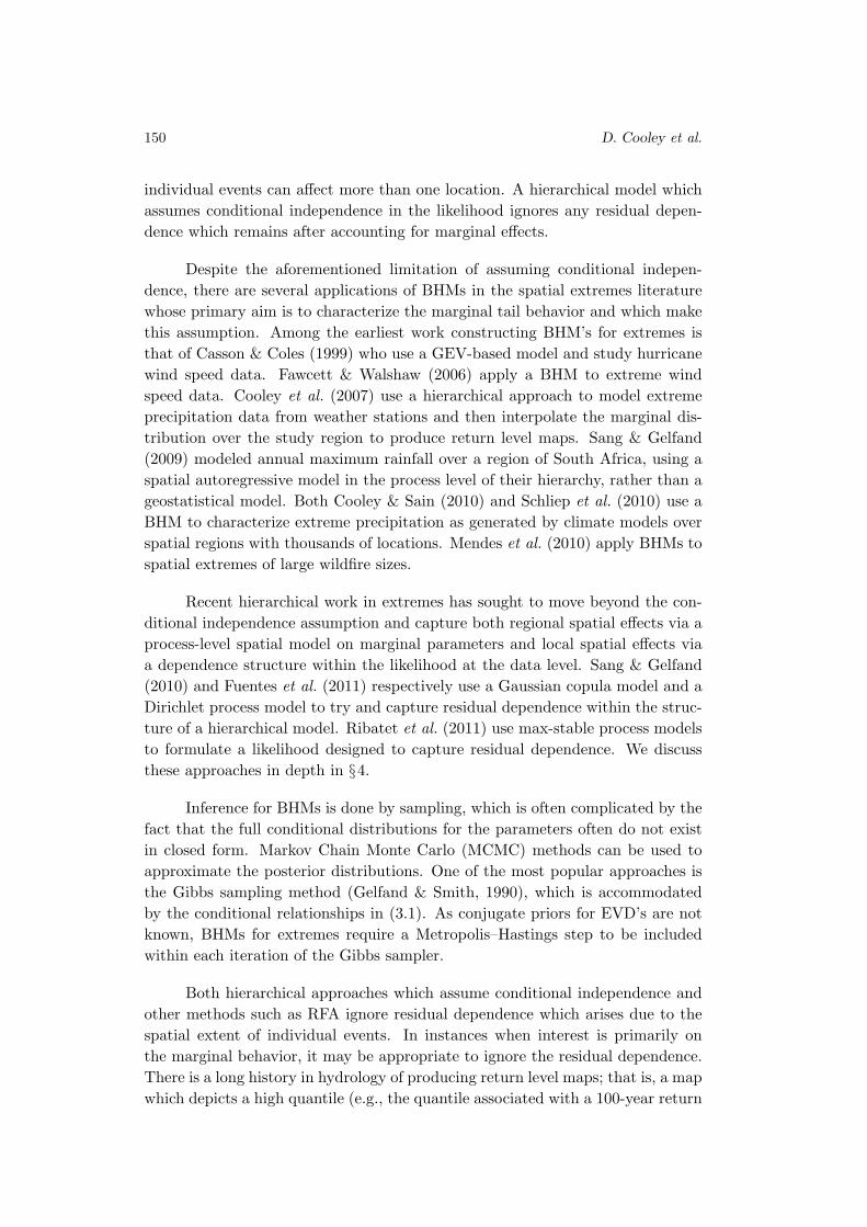
Despite the aforementioned limitation of assuming conditional indepen-

dence, there are several applications of BHMs in the spatial extremes literature

whose primary aim is to characterize the marginal tail behavior and which make

this assumption. Among the earliest work constructing BHM’s for extremes is

that of Casson & Coles (1999) who use a GEV-based model and study hurricane

wind speed data. Fawcett & Walshaw (2006) apply a BHM to extreme wind

speed data. Cooley et al. (2007) use a hierarchical approach to model extreme

precipitation data from weather stations and then interpolate the marginal dis-

tribution over the study region to produce return level maps. Sang & Gelfand

(2009) modeled annual maximum rainfall over a region of South Africa, using a

spatial autoregressive model in the process level of their hierarchy, rather than a

geostatistical model. Both Cooley & Sain (2010) and Schliep et al. (2010) use a

BHM to characterize extreme precipitation as generated by climate models over

spatial regions with thousands of locations. Mendes et al. (2010) apply BHMs to

spatial extremes of large wildfire sizes.

Recent hierarchical work in extremes has sought to move beyond the con-

ditional independence assumption and capture both regional spatial effects via a

process-level spatial model on marginal parameters and local spatial effects via

a dependence structure within the likelihood at the data level. Sang & Gelfand

(2010) and Fuentes et al. (2011) respectively use a Gaussian copula model and a

Dirichlet process model to try and capture residual dependence within the struc-

ture of a hierarchical model. Ribatet et al. (2011) use max-stable process models

to formulate a likelihood designed to capture residual dependence. We discuss

these approaches in depth in §4.

Inference for BHMs is done by sampling, which is often complicated by the

fact that the full conditional distributions for the parameters often do not exist

in closed form. Markov Chain Monte Carlo (MCMC) methods can be used to

approximate the posterior distributions. One of the most popular approaches is

the Gibbs sampling method (Gelfand & Smith, 1990), which is accommodated

by the conditional relationships in (3.1). As conjugate priors for EVD’s are not

known, BHMs for extremes require a Metropolis–Hastings step to be included

within each iteration of the Gibbs sampler.

Both hierarchical approaches which assume conditional independence and

other methods such as RFA ignore residual dependence which arises due to the

spatial extent of individual events. In instances when interest is primarily on

the marginal behavior, it may be appropriate to ignore the residual dependence.

There is a long history in hydrology of producing return level maps; that is, a map

which depicts a high quantile (e.g., the quantile associated with a 100-year return


level) at any site within a study region. The aforementioned projects by Bonnin

et al. (2004a,b) produced such maps and NOAA’s Hydrometeorological Design

Studies Center maintains a website2 which provides point-located return level es-

timates. Likewise, projects such as Cooley & Sain (2010), Sang & Gelfand (2009)

and Cooley et al. (2007) aimed only to estimate pointwise return levels. It is

imperative that it is recognized that such projects cannot be used to quantify the

aggregated effects of a large event which occurs across multiple locations, nor can

they be used to produce realistic simulated data (Davison et al., 2012, Figure 4).

4. MODELS FOR SPATIAL DEPENDENCE

In this section, we consider two approaches for capturing the residual de-

pendence assuming that the marginal effects have been accounted for. The first

approach is to use a max-stable process model (§1.1), which will assume that the

marginals have been transformed to be unit Frechet. The second is a copula ap-

proach, a popular recent approach for modeling multivariate data which assumes

the marginals are Uniform [0,1].

4.1. Max-stable processes

The definition of a max-stable process, Equation (1.4), as the infinite di-

mensional generalization of a multivariate max-stable distribution gives a well-

defined class of models, but it does not suggest how to construct such processes.

A conceptual construction of max-stable processes was first given with a spectral

representation of extremal processes by de Haan (1984) and de Haan & Ferreira

(2006). A general representation of max-stable processes can be described by two

components, a stochastic process {X(s)} and a Poisson process Π with intensity

dζ/ζ2 on (0,∞). Let {Xi(s)}i∈N be independent realizations of a process X(s)

with E[X(s)] = 1, and let ζi ∈ Π be points of the Poisson process. Then

Z(s) = maxi≥1

ζiXi(s) , s ∈ S ,

is a max-stable process with unit-Frechet margins and the distribution function

is determined by

Pr(

Z(s) ≤ z(s), s ∈ S)

= exp

(

−E[

sups∈S

{

X(s)

z(s)

}])

,

where minus the exponent is the infinite-dimensional analogue to V ; see Equation

(1.3). Different choices of the process Xi(s) lead to different classes of max-stable

processes.

2 http://hdsc.nws.noaa.gov/hdsc/pfds/index.htm


Although Gaussian distributions and processes are not well-suited for

modeling extremes, they can be used within the above max-stable construction

to produce appropriate models. This was first proposed by Smith (1990).

Let {(ζi, si); i≥ 1} denote the points of a Poisson process on (0,∞) × S with

intensity ζ−2 dζ ds. Let {f(x)} on Rd denote a non-negative function such that

∫

f(x) dx = 1 and define

Z(s) = maxiζi f(s− si) .

Then Z(·) is a max-stable process with unit-Frechet margins. Smith also intro-

duced the so-called rainfall-storms interpretation: think of f(·) as the shape of

a storm centered at point si, and think of the overall magnitude of storm as ζi.

Then the max-stable process Z(·) is the pointwise maximum rainfall (taken over

all storms) for each location in S. If f(·) is a multivariate normal density with

covariance parameter Σ, then the process Z(·) is called a Gaussian extreme value

process and the joint distribution at two sites is given by

Pr{

Z(s1) ≤ z1, Z(s2) ≤ z2

}

=

= exp

{

− 1

z1Φ

(

a

2+

1

alog

z2z1

)

− 1

z2Φ

(

a

2+

1

alog

z1z2

)

}

,

where a =√

(s1− s2)T Σ−1(s1− s2) and Φ is the standard normal cumulative

distribution function. The dependence parameter a represents a transformed

distance between two sites and the limits a→ 0 and a→ ∞ correspond to perfect

dependence and independence, respectively. Thus the most common Smith model

takes Xi(s) to be a multivariate density function. Figure 2 shows a realization.

Schlather (2002) suggested a more flexible class of max-stable processes by

taking Xi(s) to be any stationary Gaussian random field with finite expectation.

A stationary max-stable process with unit-Frechet margins can be obtained by

Z(s) = maxiζi max

{

0, Xi(s)}

where µ = E{

max(0, Xi(s))}

<∞ and {ζi} denotes the points of a Poisson pro-

cess on (0,∞) with intensity measure µ−1ζ−2 dζ. The max-stable process also

allows a useful interpretation of spatial storm events. On taking a stationary ran-

dom process Xi(s), the spatial rainfall events have the same dependence structure

but the realizations will vary stochastically, not the deterministic form f(·) such

as Smith’s model. If the random process is specified for a stationary isotropic

Gaussian random field Xi(·) with unit variance, correlation ρ(·) and µ−1 =√

2π,

then the process Z(s) is called an extremal Gaussian process and the bivariate

marginal distributions are given by

Pr{

Z(s1) ≤ z1, Z(s2) ≤ z2

}

=

= exp

{

− 1

2

(

1

z1+

1

z2

)(

1 +

√

1 − 2(

ρ(h) + 1) z1z2

(z1 + z2)2

)

}


where h is the Euclidean distance between station s1 and s2. The correlation

is chosen from one of the valid families of correlations for Gaussian processes.

Figure 2 shows a realization of an extremal Gaussian process.

One drawback to the Schlather model is that it cannot attain independence

of extremes, because the extremal coefficient θ(h) = 1+[1−ρ(h)

2

]1/2takes the value

in the interval [1, 1.838] (and not the usual range of [1,2]) as the distance h→ ∞.

To overcome this, the process Xi(s) can be restricted to a random set B, i.e.,

Z(s) = maxiζiXi(s) IBi

(s− si)

where IB is the indicator function of a compact random set B ⊂ S and si are

the points of a Poisson process on S. If Xi is a Gaussian process, the bivariate

marginal distribution is

exp

{

−(

1

z1+

1

z2

)

[

1 − α(h)

2

(

1 −√

1 − 2(

ρ(h) + 1) z1z2

(z1 + z2)2

)

]}

where α(h) = E{

|B ∩ (h+B)|}

/E(|B|) ∈ [0, 1]. The extremal coefficient takes on

any value in the interval [1, 2] and thus independent extremes are available. One

possible choice for the set B is a disc of radius r, meaning α(h).= {1−|h|/(2r)}+,

which equals 0 when |h| > 2 r. One could consider B as a random set, which means

that the radius of the disk is random and all elliptical sets having the same major

axis are permissible as a generalization for B (Davison & Gholamrezaee, 2012).

Kabluchko et al. (2009) proposed an alternative specification for the Xi(·)process, which requires weaker assumptions than second-order stationarity. Let

Xi(s) = exp{

ei(s)− 12 σ

2(s)}

where ei(s) is a Gaussian process with stationary in-

crements and σ2(s) = Var{e(s)}. Then the process, known as the Brown–Resnick

process, can be a very general class of max-stable processes which allows the use

of semivariogram from standard geostatistics. The bivariate cdf transformed to

0

5

10

15

0 2 4 6 8 10

0

2

4

6

8

10

Smith Process

0

1

2

3

4

5

6

7

0 2 4 6 8 10

0

2

4

6

8

10

Schlather Process

0

2

4

6

8

10

0 2 4 6 8 10

0

2

4

6

8

10

Brown−Resnick Process

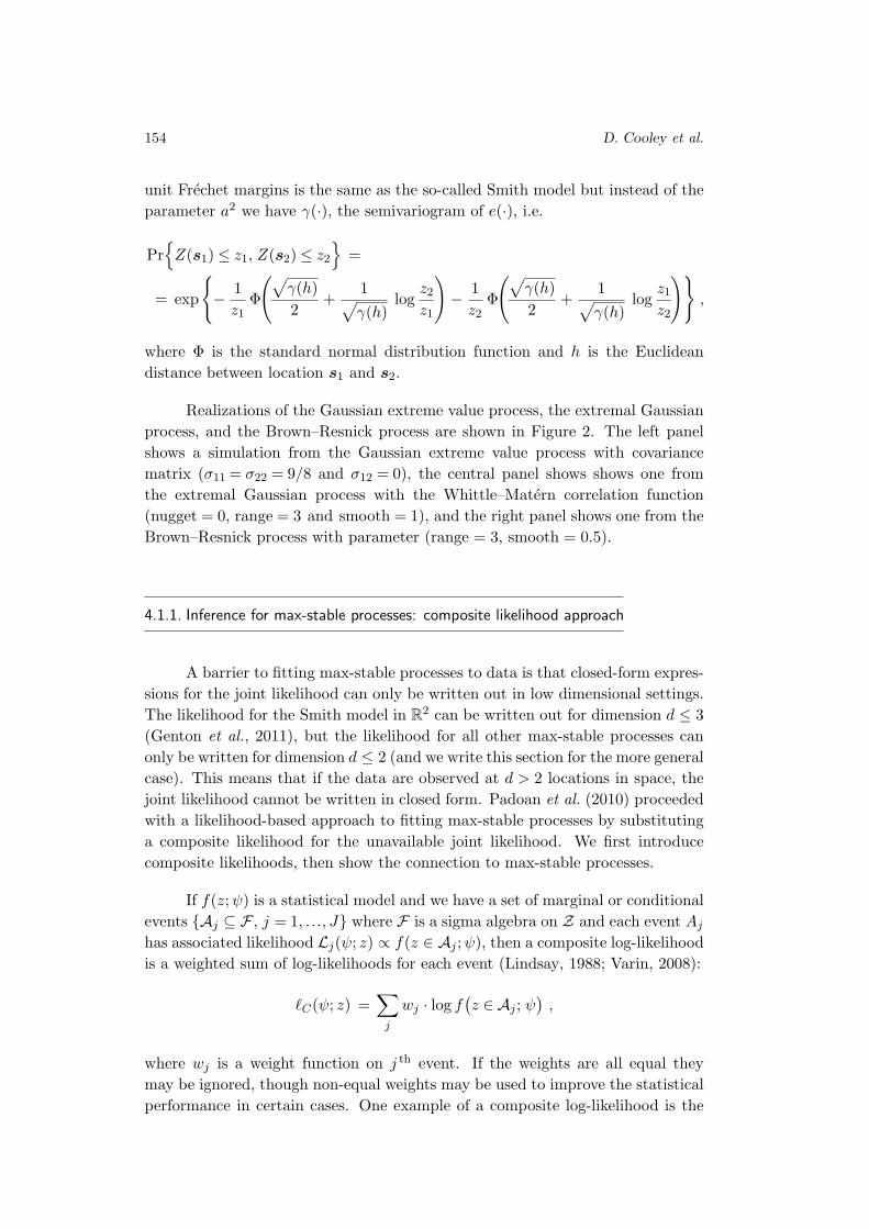
Figure 2: Realization of Gaussian extreme value process (left), extremalGaussian process (centre), and Brown–Resnick process (right)from SpatialExtremes R package (Ribatet, 2011; R Develop-ment Core Team, 2011).


unit Frechet margins is the same as the so-called Smith model but instead of the

parameter a2 we have γ(·), the semivariogram of e(·), i.e.

Pr{

Z(s1) ≤ z1, Z(s2) ≤ z2

}

=

= exp

{

− 1

z1Φ

(

√

γ(h)

2+

1√

γ(h)log

z2z1

)

− 1

z2Φ

(

√

γ(h)

2+

1√

γ(h)log

z1z2

)}

,

where Φ is the standard normal distribution function and h is the Euclidean

distance between location s1 and s2.

Realizations of the Gaussian extreme value process, the extremal Gaussian

process, and the Brown–Resnick process are shown in Figure 2. The left panel

shows a simulation from the Gaussian extreme value process with covariance

matrix (σ11 = σ22 = 9/8 and σ12 = 0), the central panel shows shows one from

the extremal Gaussian process with the Whittle–Matern correlation function

(nugget = 0, range = 3 and smooth = 1), and the right panel shows one from the

Brown–Resnick process with parameter (range = 3, smooth = 0.5).

4.1.1. Inference for max-stable processes: composite likelihood approach

A barrier to fitting max-stable processes to data is that closed-form expres-

sions for the joint likelihood can only be written out in low dimensional settings.

The likelihood for the Smith model in R2 can be written out for dimension d ≤ 3

(Genton et al., 2011), but the likelihood for all other max-stable processes can

only be written for dimension d ≤ 2 (and we write this section for the more general

case). This means that if the data are observed at d > 2 locations in space, the

joint likelihood cannot be written in closed form. Padoan et al. (2010) proceeded

with a likelihood-based approach to fitting max-stable processes by substituting

a composite likelihood for the unavailable joint likelihood. We first introduce

composite likelihoods, then show the connection to max-stable processes.

If f(z;ψ) is a statistical model and we have a set of marginal or conditional

events {Aj ⊆ F , j = 1, ..., J} where F is a sigma algebra on Z and each event Ajhas associated likelihood Lj(ψ; z) ∝ f(z ∈ Aj ;ψ), then a composite log-likelihood

is a weighted sum of log-likelihoods for each event (Lindsay, 1988; Varin, 2008):

ℓC(ψ; z) =∑

j

wj · log f(

z ∈ Aj ; ψ)

,

where wj is a weight function on j th event. If the weights are all equal they

may be ignored, though non-equal weights may be used to improve the statistical

performance in certain cases. One example of a composite log-likelihood is the


pairwise log-likelihood, defined (in a spatial application) as

ℓC(ψ; z) =m∑

k=1

d−1∑

j=1

d∑

j′=j+1

log f(

zk(sj), zk(sj′); ψ)

,

where each term f(

zk(sj), zk(sj′); ψ)

is a bivariate marginal density function

based on observations at locations j and j′, and ψ is a spatial dependence pa-

rameter. The two inner summations sum over all unique pairs, while the outer

sums over the m i.i.d. replicates. Similar to the full likelihood function, the pa-

rameter which maximizes a composite log likelihood can be found, and is termed

a maximum composite likelihood estimate, or MCLE. When m→ ∞, the max-

imum composite likelihood estimator is consistent and asymptotically normal

(Lindsay, 1988; Cox & Reid, 2004), with

(4.1) ψMCLE ∼ N (ψ, I−1) , I = H(ψ)J−1(ψ)H(ψ) ,

where H(ψ) = E(−Hψ ℓC(ψ;Z)) is the expected information matrix, J(ψ) =

V (Dψ ℓC(ψ;Z)) is the covariance of the score, Hψ is the Hessian matrix, Dψ

is the gradient vector, and V is the covariance matrix. When one has the full

likelihood, H(ψ) = J(ψ), but in the composite likelihood setting these matrices

are not equal.

Padoan et al. (2010) used the composite likelihood to model the joint spa-

tial dependence of extremes and accounted for regional effects with a regression

model on the GEV parameters. This approach is implemented in the R package

SpatialExtremes (Ribatet, 2011). The maximum composite likelihood estimator

ψMCLE is found numerically. The variance is estimated using

H(ψMCLE) = −m∑

k=1

d−1∑

j=1

d∑

j′=j+1

Hψ log f(

zk(sj), zk(sj′); ψMCLE

)

and

J(ψMCLE) =

m∑

k=1

{

d−1∑

j=1

d∑

j′=j+1

Dψ log f(


)

}

×{

d−1∑

j=1

d∑

j′=j+1

Dψ log f(


)

}

T

.

The dependence parameter ψ is generic and stands in for the matrix Σ in the

Smith model, the Gaussian correlation function ρ(h;ψ) in the Schlather model,

and the semivariogram γ(h;ψ) in the Brown–Resnick model. For each of these

models the target parameter appears in the corresponding bivariate density func-

tions, and thus also in the pairwise log-likelihood.

Recently, there has been work which begins to explore the use of composite

likelihood methods within Bayesian inference, and much of this work has been


driven by interest in spatial extremes. Both Pauli et al. (2011) and Ribatet et al.

(2011) seek to employ a pairwise likelihood, rather than the unattainable true

likelihood, to obtain a posterior distribution. The pairwise likelihood does not

accurately represent the information in the data, as it repeatedly uses each ob-

servation when pairing it with others. Pauli et al. (2011) adjust the pairwise

likelihood so that the first moment of the log-likelihood ratio corresponds to that

of the asymptotic χ2-distribution. Ribatet et al. (2011) suggest an adjustment

which ensures that the curvature of the likelihood surface agrees with the asymp-

totic covariance matrix given in Equation (4.1). Ribatet et al. (2011) apply the

likelihood within a spatial hierarchical model to study extreme precipitation in

Switzerland.

Erhardt & Smith (2011) used approximate Bayesian computing (ABC) to

obtain an approximate posterior distribution for the max-stable process depen-

dence parameters ψ. ABC methods have been successfully implemented for prob-

lems where the joint likelihood function is intractable, but simulations are possible

(Beaumont et al., 2002; Sisson & Fan, 2010). Given observed data Z and prior

π(ψ), the simplest ABC algorithm is: (1) Draw ψ′ ∼ π(ψ); (2) Simulate a new

dataset Z ′ conditional on ψ′; (3) If d(S(Z), S(Z ′)) ≤ ǫ for some summary statis-

tic S, distance function d, and threshold ǫ, then accept ψ′; otherwise, reject.

The method produces an i.i.d. sample from π[

ψ | d{S(Z), S(Z ′)} ≤ ǫ]

, which in

the limit as ǫ→ 0 equals π(ψ | S(Z)). Further, if S(Z) were a sufficient statistic,

this would be the exact posterior. In practice, computational costs often force

concessions like in-sufficient statistics S and a non-zero threshold ǫ. Erhardt &

Smith (2011) used tripletwise extremal coefficients in the construction of a sum-

mary statistic S, and then showed that the resulting ABC implementation can

outperform the composite likelihood approach when estimating the spatial depen-

dence of a max-stable process, though at an appreciably higher computational

cost.

4.1.2. Spatial prediction/interpolation for max-stable processes

Kriging is a central focus of geostatistics and there has been recent work

to perform spatial prediction for max-stable processes (§1.2). Wang & Stoev

(2011) and Dombry et al. (2011) have proposed computational solutions for the

prediction problem for max-stable processes.

Max-linear models are a subclass of the multivariate max-stable distri-

butions. Let Yi, i= 1, ..., n, be i.i.d. unit Frechet random variables. Assume

Z =(

Z(s1), ..., Z(sd))

T

is a max-linear combination of the Yi’s; that is,

Z(sj) =n∨

i=1

cj,i Yi , j = 1, ..., d ,


where cj,i are non-negative constants. Z is multivariate max-stable, and further if∑n

i=1 cj,i = 1 for all j, then Z has unit-Frechet marginals. Any max-linear model

with finite n will have a discrete angular measure; however, max-linear mod-

els form a dense subclass of multivariate max-stable random vectors as n→ ∞(Zhang & Smith, 2004). Wang & Stoev (2011) propose an algorithm for efficient

and exact sampling from the conditional distributions of a spectrally discrete

max-stable random field. The main idea is to first generate samples from the reg-

ular conditional probability distribution of Y |Z = z, where Y = (Y1, ..., Yn)T

and Z is the vector of values at observed locations. Then, the conditional dis-

tribution of Z(s0) =∨ni=1 c0,iYi can be easily obtained for any given c0,i. The

performance of the algorithm was illustrated over the discretized Smith model

for spatial extremes.

Dombry et al. (2011) also take a computational approach to spatial predic-

tion. Specifically working with the Brown–Resnick process, Dombry et al. (2011)

establish a link between the conditional distribution of this process and the mul-

tivariate log-normal distribution. Like Wang & Stoev (2011), the computational

method of Dombry et al. (2011) considers different hitting-scenarios; that is,

the possible combinations of individual events which could yield the observed

maxima. Dombry et al. (2011) illustrate their method on precipitation data from

Switzerland.

4.2. Copula approaches

Copulas provide another framework for representing the dependence struc-

ture of a multivariate distribution with known marginals. Copulas are multivari-

ate distributions with standard uniform marginal distributions, and they char-

acterize the dependence structure of a multivariate distribution from univariate

marginal distributions by defining a joining mechanism (Nelsen, 2006; Joe, 1997).

Given a d-dimensional random vector Y = (Y1, ..., Yd)T with corresponding

marginal cdfs Fi for j = 1, ..., d and joint distribution function F , a copula is

a function C : [0, 1]d −→ [0, 1] such that

(4.2) F (Y ) = C(

F1(Y1), ..., Fd(Yd))

.

If the marginal cdfs of Y are all continuous, then the copula function C is uniquely

defined by (4.2). Conversely, for a copula C and continuous margins F1, ..., Fd,

the copula C corresponds to the distribution of F1(Y1), ..., Fd(Yd), i.e.,

(4.3) C(

u1, ..., ud)

= F(

F−11 (u1), ..., F

−1d (ud)

)

.

This follows from the multi-dimensional analog of Sklar’s theorem (Sklar, 1959),

which proves the existence of a copula in the bivariate case and uniqueness when

the marginals are continuous (Nelsen, 2006).


The copula framework has appeal for modeling multivariate extremes, es-

pecially since the list of existing parametric subfamilies of the multivariate ex-

treme value distribution (MEVDs) is limited. When working with multivariate

block maximum data, extreme value theory suggests that each marginal should

be approximately GEV distributed. Equation (4.3) suggests one can combine

knowledge of the marginal distributions with a copula model to obtain a valid

cdf. Further, (4.2) says that one can obtain a copula model from any multivariate

distribution. While this approach allows one great flexibility to create multivari-

ate distributions with GEV marginals, these distributions will not correspond to

a MEVD as characterized in §1.1 unless one uses an extremal copula model (Joe,

1997), which essentially correspond to the existing parametric MEVD subfamilies.

Use of (nonextremal) copula models to describe extremes has been controversial,

and Mikosch (2006) and the associated discussion details much of the argument.

For spatial data which are typically observed at many locations, one would

need a copula which can handle high dimensions, and further, whose pairwise

dependence can be linked to distance. Two obvious choices are to use the mul-

tivariate Gaussian or multivariate Student t distributions to generate a copula.

Given a d-dimensional Gaussian random vector Y = (Y1, ..., Yd)T, the Gaussian

copula is defined as

(4.4) CΣ

(

u1, ..., ud)

= ΦΣ

(

Φ−1(u1), ...,Φ−1(ud)

)

,

where ui ∈ [0, 1] for i = 1, ..., d, Φ is the cdf for a standard normal distribu-

tion, and ΦΣ is the joint cdf of the multivariate normal distribution with co-

variance matrix Σ. The multivariate Student t distribution copula is defined

similarly, except the marginal and joint distributions displayed in (4.4) are re-

placed by marginal and joint (with scale matrix Σ) Student t distributions , i.e.,

CΣ(u1, ..., ud) = Tν;Σ(

T−1ν (u1), ..., T

−1ν (ud)

)

, where Tν;Σ and Tν are the joint and

marginal t distributions with ν degrees of freedom respectively.

The simplicity of the Gaussian and Student t copulas make them appeal-

ing, but they have some undesirable properties from the extreme value theory

viewpoint. Because neither copula is extremal, the resulting cdf will not be max-

stable. Additionally, the Gaussian copula is asymptotically independent, so it

may underestimate joint tail probabilities if the data are actually asymptotically

dependent.

Husler & Reiss (1989) devised an alternative approach which used the bi-

variate Gaussian distribution to create an extremal copula (equivalently a MEVD),

and this general approach can be used with either the multivariate Gaussian dis-

tribution or multivariate t distribution as described by Davison et al. (2012).

The approach is essentially the same as that which leads to the Smith (1990)

max-stable process model, albeit in the multivariate rather than process setting.

Thus, the drawback of the extremal Gauss or extremal t copulas is that the full

multivariate distribution cannot be written in closed form, and composite like-


lihood methods must be employed. Davison et al. (2012) fit the Gaussian and

t copulas as well as the extremal Gauss and t copulas to data which are annual

maxima and conclude that the extremal copulas have improved ability to capture

the dependence found in this data. Padoan (2011) discusses some further copula

models potentially useful in spatial extremes.

In a desire to move away from the conditional independence assumption of-

ten made in hierarchical modeling, Sang & Gelfand (2010) use a Gaussian copula

to create a likelihood function in a model structured as (3.1). Suppose that Y (s)

is an extremal spatial process at location s, e.g., Y (s) is the annual maximum of

daily rainfall measurements at location s. Then Y (s) ∼ GEV(

µ(s), σ(s), ξ(s))

.

Furthermore, Y (s) can be represented as

(4.5) Y (s) = µ(s) +σ(s)

ξ(s)

(

Z(s)ξ(s) − 1)

where Z(s) is unit-Frechet. Focusing on the underlying unit-Frechet process de-

fined at locations s1, ..., sd, Sang & Gelfand (2010) induced a dependence struc-

ture on the Z(si) for i = 1, ..., d using the Gaussian copula of (4.4). Suppose

that X(s) =(

X(s1), ..., X(sd))

is a centered spatial Gaussian process with a

correlation structure defined by the function ρ(si, sj ;ψ) for i, j = 1, ..., d. The

unit-Frechet process Z(s) is defined in terms of a transformed spatial Gaussian

process X(s) by

Z =(

G∗−1Φ(

X(s1))

, ..., G∗−1(Φ(X(sd))

)

,

where G∗ is the unit-Frechet distribution function. Given the spatial Gaus-

sian process X(s), the corresponding copula is defined as CX(u1, ..., ud) =

FX,Σρ

(

Φ−1(u1), ...,Φ−1(ud)

)

where u1, ..., ud ∈ [0, 1], FX,Σρ is the multivariate

Gaussian distribution function with a covariance matrix Σρ defined by some cor-

relation function ρ(si, sj ;ψ), i, j = 1, ..., d. Then the multivariate joint distribu-

tion of Z is

FZ(z1, ..., zd) = CX(

G∗(z1), ..., G∗(zd)

)

= FX(

Φ−1G∗(z1), ...,Φ−1G∗(zd)

)

,

where zj ∈ R, j = 1, ..., d. Sang & Gelfand (2010) considered this the first stage

of a hierarchical model, where the second stage deals with the characterizations

of µ(s), σ(s), and ξ(s) found in equation (4.5). While one could be critical of the

Gaussian copula that Sang & Gelfand (2010) employ, the approach does attempt

to account for the residual spatial dependence which remains in the data after

accounting for marginal effects, while a conditional independence assumption

ignores this dependence entirely.

An alternative copula approach for spatial extremes data is proposed by

Fuentes et al. (2011), who use a Dirichlet process (DP) copula model which is

a Bayesian, nonparametric generalization of the spatial Gaussian copula model.


The DP copula model is flexible and capable of dealing with high dimensional

data, but when combined with GEV marginal distributions does not yield a

MEVD. The DP prior is a special case of the stick-breaking prior (Sethuraman,

1994). If a distribution function is such that

(4.6) Fd=

m∑

i=1

pi δψi,

where δx denotes a Dirac measure at x, p1 = V1, pi = Vi∏

j<i(1 − Vj) with

Viiid∼ Beta(1, ν), ν > 0 and ψ1, ..., ψm

iid∼ H0, which is a centering distribution.

In the spatial setting, the spatial DP copula introduces a latent process X such

that the joint density of X =(

X(s1), ..., X(sd))

is almost surely of a countable

mixture of normals,

(4.7) f(

X |Hd, τ2)

=∞∑

i=1

pi φd(

X |ψi, τ2Id)

,

where φd( · |µ,Σ) denotes the d-dimensional multivariate normal density with

mean µ and covariance matrix Σ, pi has the same distribution as in (4.6), and

ψi =(

ψi(s1), ..., ψi(sd))

with ψi |Hd iid∼ Hd and Hd d= DP (νHd

0 ), where Hd0d=

φd(· |0,Σ). Let FX be the cdf associated with the density in (4.7). Then the

multivariate joint distribution of Y given by the copula

F (Y ) = CX

(

G∗(y1), ..., G∗(yd)

)

= FX

(

H−1s1G∗(y1), ..., H

−1sdG∗(yd)

)

,

where Hs is the cdf corresponding to the density in Equation (4.7) for Z(s).

As with the spatial Gaussian copula in Sang & Gelfand (2010), the unit-Frechet

spatial process is the transformed process defined as Y (s) = G∗−1Hs(Z(s)) but

with space-dependent parameters. The joint distribution function given by a

spatial Gaussian copula can be expressed explicitly for any given set of locations,

whereas the DP copula represents the joint distribution implicitly in a Bayesian

framework.

5. DISCUSSION

The study of spatial extremes is young, as evidenced by the fact that the

majority of the work referenced in this survey article has been done in the last

10 years, and nearly all of it in the last 20 years. The study has a well-developed

foundation in probability theory, and the field has made great strides in develop-

ing realistic models based on this theory.

We anticipate further development of methods and models for spatial

extremes, and we imagine this work will follow similar themes to recent work


in geostatistics. It remains a challenge to fit max-stable process models to data

recorded at many locations, for example climate model output which has thou-

sands of locations. Interest in large data sets has spawned geostatistics work in

Gaussian Markov random fields (Rue & Held, 2005; Lindgren et al., 2011), fixed-

rank kriging (Cressie & Johannesson, 2008), and predictive processes (Banerjee

et al., 2008). Another interest in geostatistics has been space-time modeling

(Cressie & Wikle, 2011), an area which spatial extremes modeling is only begin-

ning to address (Huser & Davison, 2012). Likewise, models with nonstationary

dependence structure (e.g., Sampson & Guttorp, 1992), models which can han-

dle spatial misalignment (e.g., Berrocal et al., 2010), and models for multivariate

spatial data (e.g., Wackernagel, 2003) have been of interest in spatial statistics

for some time, but these topics are thus far unexplored for spatial extremes.

This article has largely focused on modeling data which are block maxima,

as the spatial extremes literature to date has concentrated on such data. There is

work in progress (Jeon, 2012) to extend max-stable process models to appropri-

ately model threshold exceedance data. Spatial threshold exceedance modeling

would address the first issue that when restricting one’s attention to block max-

imum data, one is likely to discard other extreme data which could be useful

in describing the spatial extent of extreme events. Although from the classical

extreme value theory point-of-view it is natural to consider vectors of componen-

twise maxima (see §1.1), practitioners can view these vectors as artificial since

they likely do not appear in the data record.

Finally, we would be remiss in this survey if we did not mention the available

software for analyzing spatial extremes data. The R package SpatialExtremes

(Ribatet, 2011) can be used both to estimate spatial dependence and to fit max-

stable process models. The RandomFields package (Schlather, 2011) is useful for

simulating max-stable processes. The conditional simulation method of Wang &

Stoev (2011) can be found in the package maxLinear (Wang, 2010).

ACKNOWLEDGMENTS

This work was supported by the 2011–12 Program on Uncertainty

Quantification at the Statistical and Applied Mathematical Sciences Institute.

Additionally, D. Cooley was partially supported by National Science Foundation

grant DMS-0905315.


REFERENCES

Banerjee, S.; Carlin, B. & Gelfand, A. (2004). Hierarchical Modeling and Analysis

for Spatial Data, Chapman, Boca Raton.

Banerjee, S.; Gelfand, A.; Finley, A. & Sang, H. (2008). Gaussian predictiveprocess models for large spatial data sets, J. R. Statist. Soc. B, 70, 825–848.

Beaumont, M.; Zhang, W. & Balding, D. (2002). Approximate Bayesian computingin population genetics, Genetics, 162, 2025–2035.

Beirlant, J.; Goegebeur, Y.; Segers, J. & Teugels, J. (2004). Statistics of

Extremes: Theory and Applications, Wiley, New York.

Berrocal, V.; Gelfand, A. & Holland, D. (2010). A bivariate space-time down-scaler under space and time misalignment, Ann. Appl. Statist., 4, 1942–1975.

Bonnin, G.M.; Todd, D.; Lin, B.; Parzybok, T.; Yekta, M. & Riley, D. (2004a).NOAA Atlas 14, Precip. Freq. Atlas United States, Vol. 1, U.S. Dep. Comm., Nat.Oceanic Atmos. Administ, Nat. Weather Serv., Silver Spring, Maryland.

Bonnin, G.M.; Todd, D.; Lin, B.; Parzybok, T.; Yekta, M. & Riley, D. (2004b).NOAA Atlas 14, Precip. Freq. Atlas United States, Vol. 2, U.S. Dep. Comm., Nat.Oceanic Atmos. Administ, Nat. Weather Serv., Silver Spring, Maryland.

Brockwell, P. & Davis, R.A. (2002). Introduction to Time Series and Forecasting

(2nd ed.), Springer, New York.

Casson, E. & Coles, S.G. (1999). Spatial regression models for extremes, Extremes,1, 449–468.

Coles, S.G. (2001). An Introduction to Statistical Modeling of Extreme Values,Springer, London.

Coles, S.G. & Dixon, M.J. (1999). Likelihood-based inference for extreme valuemodels, Extremes, 2, 5–23.

Coles, S.G.; Heffernan, J. & Tawn, J.A. (1999). Dependence measures for extremevalue analysis, Extremes, 2, 339–365.

Cooley, D.; Davis, R.A. & Naveau, P. (2010). The pairwise beta: A flexible para-metric multivariate model for extremes, J. Mult. Anal., 101, 2103–2117.

Cooley, D.; Naveau, P. & Poncet, P. (2006). Variograms for spatial max-stablerandom fields, Lect. Notes Statist., 187, 373–390, Springer, New York.

Cooley, D.; Nychka, D. & Naveau, P. (2007). Bayesian spatial modeling of extremeprecipitation return levels, J. Am. Statist. Assoc., 102, 824–840.

Cooley, D. & Sain, S.R. (2010). Spatial hierarchical modeling of precipitation ex-tremes from a regional climate model, J. Agric. Bio. Environ. Statist., 15, 381–402.

Cox, D.R. & Reid, N. (2004). A note on pseudo-likelihood constructed from marginaldensities, Biometrika, 91, 729–737.

Cressie, N.A.C. & Johannesson, G. (2008). Fixed rank kriging for very large spatialdata sets, J. R. Statist. Soc. B, 70, 209–226.

Cressie, N.A.C. & Wikle, C. (2011). Statistics for Spatio-Temporal Data, Wiley,New York.

Cressie, N.A.C. (1993). Statistics for Spatial Data, Wiley, New York.

Dalrymple, T. (1960). Flood frequency analyses, Water supply paper 1543-a, U.S.Geological Survey, Reston, VA.

Daly, C.; Gibson, W.P.; Taylor, G.H.; Johnson, G.L. & Pasteris, P. (2002).A knowledge-based approach to the statistical mapping of climate, Clim. Res., 23,99–113.


Daly, C.; Neilson, R.P. & Phillips, D.L. (1994). A statistical topographic modelfor mapping climatological precipitation in mountainous terrain, J. Appl. Meteo., 33,140–158.

Davis, R.A. & Resnick, S.I. (1989). Basic properties and prediction of max-ARMAprocesses, Adv. Appl. Prob., 21, 781–803.

Davison, A.C. & Gholamrezaee, M.M. (2012). Geostatistics of extremes, Proc. R.

Soc. Lond. A, 468, 581–608.

Davison, A.C.; Padoan, S. & Ribatet, M. (2012). Statistical modeling of spatialextremes (with Discussion), Statist. Sci., to appear.

de Haan, L. (1984). A spectral representation for max-stable processes, Ann. Prob.,12, 1194–2004.

de Haan, L. & Ferreira, A. (2006). Extreme Value Theory, Springer, New York.

Diggle, P.J.; Tawn, J.A. & Moyeed, R.A. (1998). Model-based geostatistics (withDiscussion), Appl. Statist., 47, 299–350.

Dombry, C.; Eyi-Minko, F. & Ribatet, M. (2011). Conditional simulations of

Brown–Resnick processes, submitted.

Draisma, G.; Drees, H.; Ferreira, A. & de Haan, L. (2004). Bivariate tail esti-mation: dependence in asymptotic independence, Bernoulli, 10, 251–280.

Erhardt, R.J. & Smith, R.L. (2011). Approximate Bayesian computing for spatialextremes, Comp. Statist. Data Anal., to appear.

Fawcett, L. & Walshaw, D. (2006). A hierarchical model for extreme wind speeds,J. R. Statist. Soc. C, 15, 631–646.

Fuentes, M.; Henry, J. & Reich, B. (2011). Nonparametric spatial models forextremes: Application to extreme temperature data, Extremes, to appear.

Gelfand, A. & Smith, F. (1990). Sampling-based approaches to calculating marginaldensities, J. Am. Statist. Assoc., 85, 398–409.

Genton, M.G.; Ma, Y. & Sang, H. (2011). On the likelihood function of Gaussianmax-stable processes, Biometrika, 98, 481–488.

Guttorp, P. & Xu, J. (2011). Climate change, trends in extremes, and model assess-ment for a long temperature time series from Sweden, Environmetrics, 22, 456–463.

Heffernan, J. & Tawn, J.A. (2004). A conditional approach for multivariate extremevalues, J. R. Statist. Soc. B, 66, 497–546.

Hosking, J.R.M. & Wallis, J.R. (1997). Regional Frequency Analysis: An approach

based on L-Moments, Cambridge University Press, Cambridge.

Huser, R. & Davison, A.C. (2012). Space-time modeling of extreme events, submitted.

Husler, J. & Reiss, R. (1989). Maxima of normal random vectors: between indepen-dence and complete dependence, Statist. Prob. Lett., 7, 283–286.

Jeon, S. (2012). Max-stable Processes for Threshold Exceedances in Spatial Extremes,Ph. D. thesis, University of North Carolina at Chapel Hill.

Joe, H. (1997). Multivariate Models and Dependence Concepts (1st ed.), Chapman,New York.

Kabluchko, Z.; Schlather, M. & de Haan, L. (2009). Stationary max-stable fieldsassociated to negative definite functions, Ann. Prob., 37, 2042–2065.

Leadbetter, M.R.; Lindgren, G. & Rootzen, H. (1983). Extremes and Related

Properties of Random Sequences and Processes, Springer, New York.

Ledford, A.W. & Tawn, J.A. (1996). Statistics for near independence in multivariateextreme values, Biometrika, 83, 169–187.

Ledford, A.W. & Tawn, J.A. (1997). Modelling dependence within joint tail regions,J. R. Statist. Soc. B, 59, 475–499.


Lindgren, F.; Rue, H. & Lindstrom, J. (2011). An explicit link between Gaussianfields and Gaussian Markov random fields: the stochastic partial differential equationapproach, J. R. Statist. Soc. B, 73, 423–498.

Lindsay, B. (1988). Composite likelihood methods, Contemp. Math., 80, 221–239.

Mannshardt-Shamseldin, E.C.; Smith, R.L.; Sain, S.R.; Mearns, L.O. & Coo-

ley, D. (2010). Downscaling extremes: A comparison of extreme value distributionsin point-source and gridded precipitation data, Ann. Appl. Statist., 4, 484–502.

Matheron, G. (1987). Suffit-il, pour une covariance, d’etre de type positif? Sciences

Terre, Serie Inform. Geo., 26, 51–66.

Mendes, J.M.; de Zea Bermudez, P.C. & Pereira, J. (2010). Spatial extremes ofwildfire sizes: Bayesian hierarchical models for extremes, Environ. Ecol. Statist., 17,1–28.

Mikosch, T. (2006). Copulas: Tales and facts, Extremes, 9, 3–20.

Naveau, P.; Guillou, A.; Cooley, D. & Diebolt, J. (2009). Modeling pairwisedependence of maxima in space, Biometrika, 96, 1–17.

Nelsen, R.B. (2006). An Introduction to Copulas (2nd ed.), Springer, New York.

Padoan, S.A. (2011). Multivariate extreme models based on underlying skew-t andskew-normal distributions, J. Mult. Anal., 102, 977–991.

Padoan, S.A.; Ribatet, M. & Sisson, S.A. (2010). Likelihood-based inference formax-stable processes, J. Am. Statist. Assoc., 105, 263–277.

Pauli, F.; Racugno, W. & Ventura, L. (2011). Bayesian composite marginal like-lihoods, Statist. Sinica, 21, 149–164.

Peng, L. (1999). Estimation of the coefficient of tail dependence in bivariate extremes,Statist. Prob. Lett., 43, 399–409.

R Development Core Team (2011). R: A Language and Environment for Statistical

Computing, R Foundation for Statistical Computing, Vienna, Austria.

Ramos, A. & Ledford, A.W. (2009). A new class of models for bivariate joint tails,J. R. Statist. Soc. B, 71, 219–241.

Resnick, S.I. (1987). Extreme Values, Regular Variation, and Point Processes, Springer,New York.

Ribatet, M. (2011). SpatialExtremes: Modelling Spatial Extremes, R package version1.8-1.

Ribatet, M.; Cooley, D. & Davison, A.C. (2011). Bayesian inference for com-posite likelihood models and an application to spatial extremes, Statist. Sinica

(doi:10.5705/ss.2009.248).

Rue, H. & Held, L. (2005). Gaussian Markov Random Fields: Theory and Applica-

tions, Chapman, Boca Raton.

Sampson, P. & Guttorp, P. (1992). Nonparametric estimation of nonstationary spa-tial covariance structure, J. Am. Statist. Assoc., 47, 108–119.

Sang, H. & Gelfand, A.E. (2009). Hierarchical modeling for extreme values observedover space and time, Environ. Ecol. Statist., 16, 407–426.

Sang, H. & Gelfand, A.E. (2010). Continuous spatial process models for spatialextreme values, J. Agric. Bio. Environ. Statist., 15, 49–65.

Schabenberger, O. & Gotway, C.A. (2005). Statistical Methods for Spatial Data

Analysis, Chapman, Boca Raton.

Schlather, M. (2002). Models for stationary max-stable random fields, Extremes, 5,33–44.

Schlather, M. (2011). RandomFields: Simulation and Analysis of Random Fields,R package version 2.0.53.

Schlather, M. & Tawn, J.A. (2002). Inequalities for the extremal coefficients ofmultivariate extreme value distributions, Extremes, 5, 87–102.


Schlather, M. & Tawn, J.A. (2003). A dependence measure for multivariate andspatial extreme values: Properties and inference, Biometrika, 90, 139–156.

Schliep, E.; Cooley, D.; Sain, S. & Hoeting, J. (2010). A comparison study of ex-treme precipitation from six regional climate models via spatial hierarchical modeling,Extremes, 13, 219–239.

Sethuraman, J. (1994). A constructive definition of Dirichlet priors, Statist. Sinica, 4,639–650.

Sibuya, M. (1960). Bivariate extremal distribution, Ann. Inst. Statist. Math., 11, 195–210.

Sisson, S. & Fan, Y. (2010). Likelihood-free Markov chain Monte Carlo. In “Handbookof Markov Chain Monte Carlo” (S. Brooks, A. Gelman, G. Jones and X. Meng, Eds.),pp. 319–341, Chapman, Boca Raton.

Sklar, A. (1959). Fonctions de repartition a n dimensions et leurs marges, Publications

de l’Institut de Statistique de l’Universite de Paris, 8, 229–231.

Smith, R.L. (1990). Max-stable processes and spatial extremes, unpublished manuscript.

Varin, C. (2008). On composite marginal likelihoods, Adv. Statist. Anal., 92, 1–28.

Wackernagel, H. (2003). Multivariate Geostatistics, An Introduction with Applica-

tions (3rd ed.), Springer, Berlin.

Wang, Y. (2010). maxLinear: Conditional Sampling for Max-Linear Models, R packageversion 1.0.

Wang, Y. & Stoev, S.A. (2011). Conditional sampling for spectrally discrete max-stable random fields, Adv. Appl. Prob., 43, 461–483.

Zhang, Z. & Smith, R.L. (2004). The behavior of multivariate maxima of movingmaxima processes, J. Appl. Prob., 41, 1113–1123.

Documents

ASURVEYOFSPATIALEXTREMES:MEASURINGSPATIAL DEPENDENCE AND ... · ASURVEYOFSPATIALEXTREMES:MEASURINGSPATIAL DEPENDENCE AND MODELING SPATIAL ... lies at the intersection of two branches