Attribution of Projected Changes in Atmospheric Moisture Transport in the Arctic:A Self-Organizing Map Perspective

NATASA SKIFIC

Department of Atmospheric Sciences, Rutgers, The State University of New Jersey, New Brunswick, New Jersey

JENNIFER A. FRANCIS

Institute of Marine and Coastal Sciences, Rutgers, The State University of New Jersey, New Brunswick, New Jersey

JOHN J. CASSANO

Department of Atmospheric and Oceanic Sciences, and Cooperative Institute for Research in Environmental Sciences,

University of Colorado, Boulder, Colorado

(Manuscript received 27 May 2008, in final form 18 February 2009)

ABSTRACT

Meridonal moisture transport into the Arctic derived from one simulation of the National Center for

Atmospheric Research Community Climate System Model (CCSM3), spanning the periods of 1960–99,

2010–30, and 2070–89, is analyzed. The twenty-first-century simulation incorporates the Intergovernmental

Panel on Climate Change (IPCC) Special Report on Emission Scenarios (SRES) A2 scenario for CO2 and

sulfate emissions. Modeled and observed [from the 40-yr ECMWF Re-Analysis (ERA-40)] sea level pressure

(SLP) fields are classified using a neural network technique called self-organizing maps to distill a set of

characteristic atmospheric circulation patterns over the region north of 608N. Model performance is validated

for the twentieth century by comparing the frequencies of occurrence of particular circulation regimes in the

model to those from the ERA-40. The model successfully captures dominant SLP patterns, but differs from

observations in the frequency with which certain patterns occur. The model’s twentieth-century vertical

mean moisture transport profile across 708N compares well in terms of structure but exceeds the observations

by about 12% overall. By relating moisture transport to a particular circulation regime, future changes in

moisture transport across 708N are assessed and attributed to changes in frequency with which the atmo-

sphere resides in particular SLP patterns and/or to other factors, such as changes in the meridional moisture

gradient. By the late twenty-first century, the transport is projected to increase by about 21% in this model

realization, with the largest contribution (32%) to the total change occurring in summer. Only about one-

quarter of the annual increase is due to changes in pattern occupancy, suggesting that the majority is related

to mainly thermodynamic factors. A larger poleward moisture transport likely constitutes a positive feedback

on the system through related increases in latent heat release and the emission of longwave radiation to the

surface.

1. Introduction

The Fourth Assessment Report (AR4) of the Inter-

governmental Panel on Climate Change (IPCC; Solomon

et al. 2007) underscores previous striking and disturbing

findings: the Arctic system appears to be heading toward

a new state, and there are no apparent feedbacks within

the Arctic that can arrest the cohesive change (Ferguson

et al. 2004; Overpeck et al. 2005; Serreze and Francis

2006). Although there is a great deal of uncertainty

related to feedbacks in the Arctic system, particularly

involving cloud changes, it appears that the over-

whelming majority of them are positive, that is, they act

to enhance changes (Serreze and Barry 2005). The most

often cited of these are the ice/snow albedo feedback

and water vapor feedback. The basic process in the

former is that as high-latitude temperatures increase,

additional sea ice and snow will melt, which will expose

dark ocean and land surfaces that are more effective ab-

sorbers of solar radiation. This will increase the warming,

Corresponding author address: Jennifer A. Francis, IMCS,

Rutgers University, 71 Dudley Rd., New Brunswick, NJ 08901.

E-mail: francis@imcs.rutgers.edu

1 AUGUST 2009 S K I F I C E T A L . 4135

DOI: 10.1175/2009JCLI2645.1

� 2009 American Meteorological Society

leading to further melt of snow and ice, and hence fur-

ther warming. Because most of the Arctic surface is

covered with ice and snow during spring, the effects will

be most pronounced in high latitudes (Hartmann 1994).

The water vapor feedback involves an increase in pre-

cipitable water in the atmosphere as warming raises the

saturation vapor pressure. Increased precipitable water

enhances the emissivity of the atmosphere, which tends to

increase the longwave flux to the surface, particularly in

dry atmospheres like the polar regions (Soden and Held

2006). While these feedbacks seem straightforward, the

processes by which energy is sequestered in the system

until the following year are not well understood. There are

only a few known or suspected negative feedbacks within

the Arctic system. The aerosol dehydration feedback

(Blanchet and Girard 1995) is a possibility, but it is likely

too weak to have a discernible effect. Slowing of the

thermohaline circulation in response to increased fresh-

water export to the North Atlantic is likely to have a

dampening effect, but the time scales are too slow to have

a substantial impact in the near term (Fichefet et al. 2003).

In this study we investigate a potentially influential

but poorly understood feedback that extends beyond

the Arctic and involves the horizontal transport of moist

static energy (sensible heat, latent heat, and geopotential

energy) from low to high latitudes by the atmosphere. In

the present climate, the moist static energy transport

supplies approximately 98% of the energy annually lost

to space by the Arctic north of 708N (Nakamura and

Oort 1988). Because the Arctic warms more than lower

latitudes, one expects that the lower-tropospheric me-

ridional temperature gradient should relax, poleward

advection of sensible heat should decrease, and Arctic

warming should weaken. Simulations with global cli-

mate models support this reasoning, but they also sug-

gest that increases in moisture transport will more than

compensate for the reduction in sensible heat transport

(S. Vavrus 2007, personal communication). Recent an-

alyses by Graversen et al. (2008), and earlier work by

Alexeev et al. (2005) and Held and Soden (2006), sup-

port the notion that meridional energy transport may

enhance Arctic warming. Other studies reveal possible

linkages between high-latitude atmospheric circulation

and tropical surface temperatures (e.g., Cassou and

Terray 2001; Hoerling et al. 2004; Hurrell et al. 2004),

but connections between tropical variations and pole-

ward transport of moisture are unclear. It is also sug-

gested that changing energy transport, perhaps in

magnitude and/or in spatial distribution, may be partly

responsible for observed reductions in Arctic sea ice

extent (Rigor and Wallace 2004), increases in surface

temperature (Comiso 2003), lengthening of the melt

season (Belchansky et al. 2004), loss of permafrost

(Osterkamp and Romanovsky 1999), and increases in

river runoff (Peterson et al. 2002).

This study explores how meridional moisture flux

across 708N changes in a single run of the National Center

for Atmospheric Research (NCAR) Community Climate

System Model, version 3 (CCSM3) over the next 100 yr,

forced with continually increasing anthropogenic green-

house gases. We apply a neural network technique called

self-organizing maps (SOMs; Kohonen 2001) for this

analysis because it distills voluminous fields of gridded

values into representative, fundamental clusters orga-

nized in a matrix of 2D fields—geographic maps in this

case—that are expressed in a visual and intuitive ren-

dering. The maps are situated in the matrix relative to

one another according to their similarity. In this appli-

cation, the fields of data are sea level pressure (SLP)

anomalies north of 608N from both reanalyses and from

the CCSM3. Each pattern in the SOM matrix is readily

identifiable as having typical atmospheric features in a

region, and inferences can be made about the weather

generally associated with those features. The SOM can

also be used to analyze other related variables, which is

the approach taken in this study to assess patterns of

moisture flux and moisture convergence (Skific et al.

2009), and ultimately to ascertain the causes of change

in these variables in the future.

The datasets used and the data manipulation that

precedes the actual application of the SOM algorithm

are described in section 2, while section 3 provides a

more in-depth description of the SOM method. Analysis

of self-organizing maps of SLP and model validation

using the 40-yr European Centre for Medium-Range

Weather Forecasts (ECMWF) Re-Analysis is summa-

rized in section 4. The analysis of the corresponding

clusters of moisture transport across 708N, fixed for a

particular circulation regime, and its comparison to

ERA-40 is given in section 5. Future changes of mois-

ture transport in the twenty-first century and derivation

of contributions of dynamic, thermodynamic, and com-

bined fractions of change are provided in section 6,

followed by conclusions and future efforts in section 7.

2. Data sources and model output

Six-hourly, multilevel fields of specific humidity and

meridional wind for a single run of the NCAR CCSM3

(version 3.0, T85 L26 resolution) were obtained from

the Program for Climate Model Diagnostics and Inter-

comparison (PCMDI), at the Lawrence Livermore Na-

tional Laboratory. CCSM3 simulations have been shown

to reproduce the Arctic atmospheric hydrological cycle

reasonably well (e.g., Holland et al. 2007; Finnis et al.

2009a,b). The atmospheric component of the model

4136 J O U R N A L O F C L I M A T E VOLUME 22

consists of 26 vertical levels, with a top at 2.2 hPa,

13 layers above 200 hPa, and a horizontal resolution of

about 1.48. The atmospheric module is the Community

Atmosphere Model (CAM) version 3.0 (Collins et al.

2006). The twentieth-century experiment (20C3M) in-

corporates the direct effect of sulfates (Smith et al. 2001,

2004), with no indirect aerosol effects. The model is forced

by observed concentrations of CO2, CH4, N2O, chloro-

fluorocarbons (CFCs), ozone (Kiehl et al. 1999), and solar

fluxes (Lean et al. 2002). The effects of volcanic eruptions

are parameterized (Ammann et al. 2003). The twenty-

first-century simulation incorporates the Special Report

on Emission Scenarios (SRES) A2 scenario (Nakicemovic

and Swart 2000), which assumes a continuously increasing

population (15 billion by 2100), increasing greenhouse

gases, and slow implementation of new technologies, and

appears to be most similar to the trajectory of the real

world (Rahmstorf et al. 2007; Pielke et al. 2008).

The original 6-hourly PCMDI fields were interpo-

lated from the hybrid sigma-pressure vertical coordi-

nates to a pressure coordinate system and reduced in

size by subsetting from global coverage to the region

north of 608N, from 6-hourly time resolution to daily

resolution (1200 UTC only) and from 26 vertical levels

to 10 levels (troposphere only). Moisture transport

was calculated for five tropospheric layers (1000–850,

850–700, 700–500, 500–400, and 400–300 hPa). The time

slices used in this study span periods of 1960–99 from

the twentieth-century experiment (20C3M), as well as

2010–30 and 2070–89 from the SRES A2 scenario. The

latter two periods were chosen to be consistent with

results from the Arctic Climate Assessment Report

(Huntington and Fox 2005; Serreze and Francis 2006) to

represent the so-called emerging and mature green-

house states. The SLP fields are also extracted for the

same time periods and interpolated from the original

1.48 3 1.48 grid to a 200 km 3 200 km Equal Area-

Scalable Earth (EASE) grid (Armstrong et al. 1997),

covering the area north of 608N and consisting of

51 3 51 grid points. (The interpolation code was ob-

tained online from http://nsidc.org/data/ease/.) Inter-

polation to an equal area grid avoids errors that might

occur because of unequal weighting of the original

latitude–longitude grid boxes in the self-organizing map

algorithm, described in the next section.

Daily SLP fields from ERA-40 (Uppala et al. 2005) were

used to validate the twentieth-century CCSM3 simulation.

The fields from 1958 to 2001 were also interpolated to the

same EASE grid prior to applying the SOM algorithm.

3. SOM methodology

SOMs provide a means to visualize the complex dis-

tribution of synoptic states (Hewitson and Crane 2002).

This technique includes an unsupervised learning al-

gorithm to reduce the dimension of large datasets by

grouping similar multidimensional fields together and

organizing them into a two-dimensional array (Kohonen

2001). In this study, the high-dimensional data subjected

to SOM analysis are fields of daily SLP anomalies from

CCSM3 for three time slices and ERA-40 on a 51 3 51

EASE grid over the region north of 608N.

The SOM consists of a 2D grid of nodes. Each node i

corresponds to an n-dimensional weight or reference

vector mi, where n is the dimension of the input data,

treated as a vector created from the grid points in each

sample. The initial step of this routine is the creation of

a first-guess array, which consists of an arbitrary number

of nodes and corresponding reference vectors. In this

study we use a grid of 35 nodes, creating a 7 3 5 array.

Slightly smaller and larger SOM matrices were tested to

determine a suitable number of nodes for this analysis.

If the matrix is too small, some characteristic atmo-

spheric patterns may not be represented; if it is too big,

adjacent patterns will be too similar and visualization is

unwieldy. The 7 3 5 matrix appears to capture and

separate the important differences in pressure patterns.

Moreover, the results are not affected by small differ-

ences in the matrix size. The reference vectors are cre-

ated at the beginning using linear initialization, which

consists of first determining the two eigenvectors with the

largest eigenvalues, and then letting these eigenvectors

span the two-dimensional linear subspace (Kohonen

2001). We use the covariance matrix of the input SLP

dataset to determine the two eigenvectors. In this case

the centroid of a rectangular array of initial reference

vectors identified with array points corresponds to the

mean of the sea level pressure values, and the vectors

identified with the corners of the array correspond to

the largest eigenvalues. By initiating a SOM in this way,

the procedure starts with an already ordered set of

weights, and then training begins with the convergence

phase. Linear initialization helps achieve faster con-

vergence, which is an advantage of this procedure over

other methods, but the SOM results are not sensitive to

the selected initialization method. In the process of

training, each data sample (i.e., one daily map of SLP) is

presented to the SOM in the order that it occurs in the

original dataset. The similarity between the data sample

and each of the reference vectors is then calculated,

usually as a measure of Euclidean distance in space.

In this process, the ‘‘best match’’ node is identified as

that with the smallest Euclidean distance between its

reference vector and the data sample. Only the vectors

for the best-matching node and those that are topolog-

ically close to it in the two-dimensional array are up-

dated. The updating scheme is shown below:

1 AUGUST 2009 S K I F I C E T A L . 4137

mi(t 1 1) 5 m

i(t) 1 h

ci(t)[x(t)�m

i(t)]

where t is a discrete time coordinate, mi is a reference

vector, x is a data sample, and hci is a neighborhood

function (Kohonen 2001), usually in the form of the

Gaussian function,

hci

5 a(t) exp �r

c� r

i

�� ��2

2s2(t)

" #,

where a is the training rate function (usually an inverse

function of time), r is the location vector in the matrix,

the distance krc 2 rik corresponds to the distance be-

tween the best-matching node (location rc) and each of

the other nodes (location ri) in the two-dimensional

matrix, and s defines the width of the kernel, or a rel-

ative distance between nodes, often referred to as the

radius of training. The training procedure is controlled

by the training rate a, the training radius s, and the

duration of training, which is fixed at 20 times the

number of data samples. The initial value of s is 4, and

decreases linearly in time. The training scheme is re-

peated several times, with the training rate reduced by an

order of magnitude each time. At the end of each trial

the mean quantization error is calculated, defined as

mqe 5

ffiffiffiffiffiffiffiffiffiffiffiffiffiffiffiffiffiffiffiffiffiffiffiffiffiffiffiffi�M

i51(x

i�m

c)2

s

M,

where xi is a data sample, M is the number of samples,

and mc is its best-matching unit out of 35 reference

vectors. A smaller mean quantization error indicates

a closer resemblance between mc and the daily SLP

anomaly fields. The training is complete once the small-

est mean quantization error is identified, because the

reference vectors from that training best approximate

the data space of interest. The final reference vectors

are then mapped onto a 2D grid, with their locations in

the matrix corresponding to their matching nodes. The

maps in the resulting matrix represent the predominant

patterns in which the atmosphere tends to reside, or

alternatively the centroid of the particular data cluster.

Although the measure of similarity between the data

and the reference vector is linear, it is this iterative

training procedure that allows the SOM to account for

the nonlinear data distributions (Hewitson and Crane

2002). The nonlinear approximation of the data space is

therefore a great advantage of the method compared to

some other approaches, such as empirical orthogonal

functions (EOFs; Reusch et al. 2005).

4. SOM of CCSM3 and ERA-40 Arctic sea levelpressure fields

a. Twentieth-century analysis

Daily sea level pressure fields from ERA-40 (1958–

2001) and CCSM3 for periods of 1960–99, 2010–30, and

2070–89 for the region north of 608N are used to create

the master SOM. Daily SLP anomalies are derived by

subtracting the gridpoint SLP from the domain-averaged

SLP for each daily field (Cassano et al. 2007). The

spatial distribution of the daily SLP anomalies represent

the SLP gradient, and thus the circulation, but are not

influenced by the absolute SLP values. Areas with ele-

vation higher than 500 m are removed from the fields

because pressure reduction to sea level can lead to un-

realistic singularities emerging in the SOM training,

which then obscure the realistic patterns.

Once a SOM of sea level pressure has been created

from the combined sets of both ERA-40 and CCSM3

SLP anomalies (hereafter the master SOM), all daily

SLP anomaly fields may be mapped to the best-matching

pattern in the master SOM to form clusters of daily

maps. This is achieved by finding the trained reference

vector associated with a node that minimizes the Eu-

clidean distance, or the squared difference, between

itself and the data sample. Once all of the samples have

been assigned to a node in the SOM, the frequencies of

occurrence can be determined, that is, the fraction of

daily fields that reside in each cluster.

Ascribing a particular daily SLP sample to a specific

circulation pattern in the SOM can also be useful for

analyzing associated variables for the same days as

those in each cluster. By mapping the new variable onto

a particular SLP pattern, the new SOM representation

can be used to describe the conditions associated with a

specific circulation regime. In section 5 we apply this

approach to fields of moisture flux across 708N.

Figure 1 presents the master SOM for SLP anomalies

north of 608N, which is derived using the combined

ERA-40 and CCSM3 SLP daily fields. These are the

dominant circulation patterns in which the atmosphere

tends to reside, according to these datasets. In the bot-

tom right are patterns with a strong Icelandic low and a

moderate-to-strong Aleutian low, with high pressure

over the northern Eurasian continent. The upper-right

part of the map is dominated by pronounced low pres-

sure in the Atlantic sector extending into Barents Sea,

while the western central Arctic, continental regions,

and the Pacific sector are dominated by high pressure.

These patterns represent a moderate or strong Beaufort

high in the winter. The bottom-left corner of the SOM

is characterized by a pronounced low pressure area in

the central Arctic with high pressure over northwestern

4138 J O U R N A L O F C L I M A T E VOLUME 22

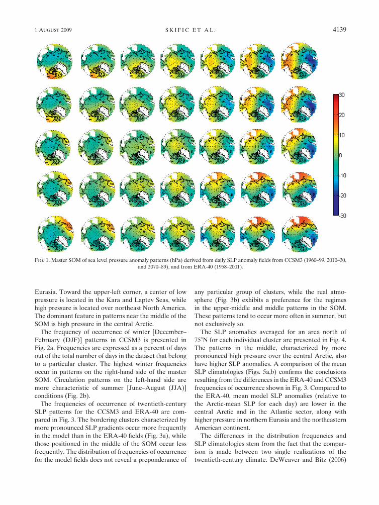
Eurasia. Toward the upper-left corner, a center of low

pressure is located in the Kara and Laptev Seas, while

high pressure is located over northeast North America.

The dominant feature in patterns near the middle of the

SOM is high pressure in the central Arctic.

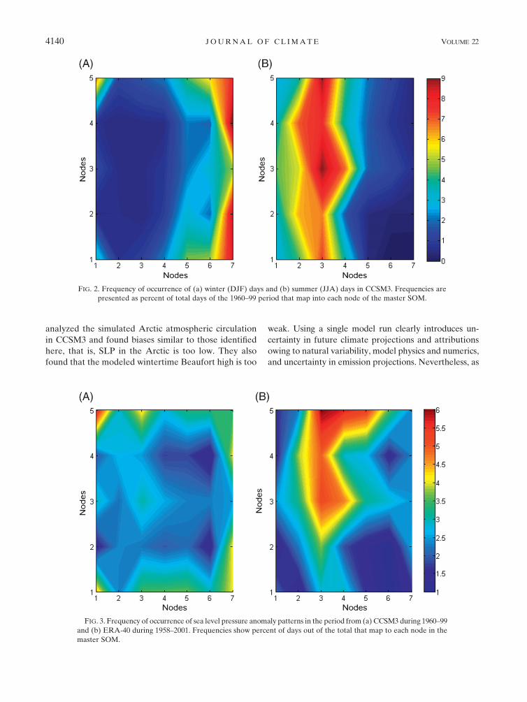
The frequency of occurrence of winter [December–

February (DJF)] patterns in CCSM3 is presented in

Fig. 2a. Frequencies are expressed as a percent of days

out of the total number of days in the dataset that belong

to a particular cluster. The highest winter frequencies

occur in patterns on the right-hand side of the master

SOM. Circulation patterns on the left-hand side are

more characteristic of summer [June–August (JJA)]

conditions (Fig. 2b).

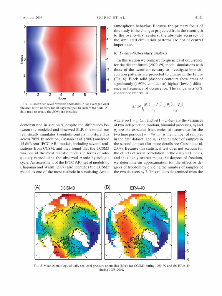
The frequencies of occurrence of twentieth-century

SLP patterns for the CCSM3 and ERA-40 are com-

pared in Fig. 3. The bordering clusters characterized by

more pronounced SLP gradients occur more frequently

in the model than in the ERA-40 fields (Fig. 3a), while

those positioned in the middle of the SOM occur less

frequently. The distribution of frequencies of occurrence

for the model fields does not reveal a preponderance of

any particular group of clusters, while the real atmo-

sphere (Fig. 3b) exhibits a preference for the regimes

in the upper-middle and middle patterns in the SOM.

These patterns tend to occur more often in summer, but

not exclusively so.

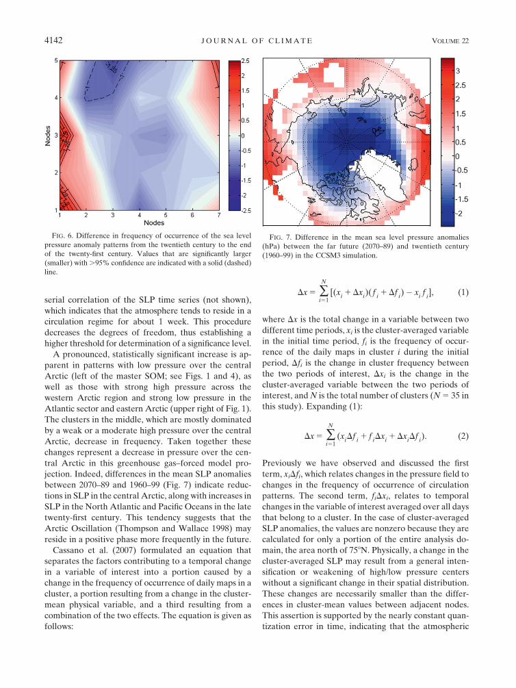
The SLP anomalies averaged for an area north of

758N for each individual cluster are presented in Fig. 4.

The patterns in the middle, characterized by more

pronounced high pressure over the central Arctic, also

have higher SLP anomalies. A comparison of the mean

SLP climatologies (Figs. 5a,b) confirms the conclusions

resulting from the differences in the ERA-40 and CCSM3

frequencies of occurrence shown in Fig. 3. Compared to

the ERA-40, mean model SLP anomalies (relative to

the Arctic-mean SLP for each day) are lower in the

central Arctic and in the Atlantic sector, along with

higher pressure in northern Eurasia and the northeastern

American continent.

The differences in the distribution frequencies and

SLP climatologies stem from the fact that the compar-

ison is made between two single realizations of the

twentieth-century climate. DeWeaver and Bitz (2006)

FIG. 1. Master SOM of sea level pressure anomaly patterns (hPa) derived from daily SLP anomaly fields from CCSM3 (1960–99, 2010–30,

and 2070–89), and from ERA-40 (1958–2001).

1 AUGUST 2009 S K I F I C E T A L . 4139

analyzed the simulated Arctic atmospheric circulation

in CCSM3 and found biases similar to those identified

here, that is, SLP in the Arctic is too low. They also

found that the modeled wintertime Beaufort high is too

weak. Using a single model run clearly introduces un-

certainty in future climate projections and attributions

owing to natural variability, model physics and numerics,

and uncertainty in emission projections. Nevertheless, as

FIG. 2. Frequency of occurrence of (a) winter (DJF) days and (b) summer (JJA) days in CCSM3. Frequencies are

presented as percent of total days of the 1960–99 period that map into each node of the master SOM.

FIG. 3. Frequency of occurrence of sea level pressure anomaly patterns in the period from (a) CCSM3 during 1960–99

and (b) ERA-40 during 1958–2001. Frequencies show percent of days out of the total that map to each node in the

master SOM.

4140 J O U R N A L O F C L I M A T E VOLUME 22

demonstrated in section 5, despite the differences be-

tween the modeled and observed SLP, this model run

realistically simulates twentieth-century moisture flux

across 708N. In addition, Cassano et al. (2007) analyzed

15 different IPCC AR4 models, including several real-

izations from CCSM, and they found that the CCSM3

was one of the most realistic models in terms of ade-

quately reproducing the observed Arctic hydrologic

cycle. An assessment of the IPCC AR4 set of models by

Chapman and Walsh (2007) also identifies the CCSM3

model as one of the most realistic in simulating Arctic

atmospheric behavior. Because the primary focus of

this study is the changes projected from the twentieth

to the twenty-first century, the absolute accuracy of

the simulated circulation patterns are not of central

importance.

b. Twenty-first-century analysis

In this section we compare frequencies of occurrence

for the distant future (2070–89) model simulations with

those of the twentieth century to investigate how cir-

culation patterns are projected to change in the future

(Fig. 6). Black solid (dashed) contours show areas of

significantly (.95% confidence) higher (lower) differ-

ence in frequency of occurrence. The range in a 95%

confidence interval is

61.96

ffiffiffiffiffiffiffiffiffiffiffiffiffiffiffiffiffiffiffiffiffiffiffiffiffiffiffiffiffiffiffiffiffiffiffiffiffiffiffiffiffiffiffiffiffiffiffiffiffiffip

1(1� p

1)

n1

1p

2(1� p

2)

n2

s,

where p1(1 2 p1)/n1 and p2(1 2 p2)/n2 are the variances

of two independent, random, binomial processes, p1 and

p2 are the expected frequencies of occurrence for the

two time periods (p 5 1/35), n1 is the number of samples

in the first dataset, and n2 is the number of samples in

the second dataset (for more details see Cassano et al.

2007). Because this statistical test does not account for

the effects of serial correlation in the daily SLP fields,

and thus likely overestimates the degrees of freedom,

we determine an approximation for the effective de-

grees of freedom by dividing the number of samples of

the two datasets by 7. This value is determined from the

FIG. 4. Mean sea level pressure anomalies (hPa) averaged over

the area north of 758N for all days mapped to each SOM node. All

data used to create the SOM are included.

FIG. 5. Mean climatology of daily sea level pressure anomalies (hPa): (a) CCSM3 during 1960–99 and (b) ERA-40

during 1958–2001.

1 AUGUST 2009 S K I F I C E T A L . 4141

serial correlation of the SLP time series (not shown),

which indicates that the atmosphere tends to reside in a

circulation regime for about 1 week. This procedure

decreases the degrees of freedom, thus establishing a

higher threshold for determination of a significance level.

A pronounced, statistically significant increase is ap-

parent in patterns with low pressure over the central

Arctic (left of the master SOM; see Figs. 1 and 4), as

well as those with strong high pressure across the

western Arctic region and strong low pressure in the

Atlantic sector and eastern Arctic (upper right of Fig. 1).

The clusters in the middle, which are mostly dominated

by a weak or a moderate high pressure over the central

Arctic, decrease in frequency. Taken together these

changes represent a decrease in pressure over the cen-

tral Arctic in this greenhouse gas–forced model pro-

jection. Indeed, differences in the mean SLP anomalies

between 2070–89 and 1960–99 (Fig. 7) indicate reduc-

tions in SLP in the central Arctic, along with increases in

SLP in the North Atlantic and Pacific Oceans in the late

twenty-first century. This tendency suggests that the

Arctic Oscillation (Thompson and Wallace 1998) may

reside in a positive phase more frequently in the future.

Cassano et al. (2007) formulated an equation that

separates the factors contributing to a temporal change

in a variable of interest into a portion caused by a

change in the frequency of occurrence of daily maps in a

cluster, a portion resulting from a change in the cluster-

mean physical variable, and a third resulting from a

combination of the two effects. The equation is given as

follows:

Dx 5 �N

i51[(x

i1 Dx

i)(f

i1 Df

i)� x

if

i], (1)

where Dx is the total change in a variable between two

different time periods, xi is the cluster-averaged variable

in the initial time period, fi is the frequency of occur-

rence of the daily maps in cluster i during the initial

period, Dfi is the change in cluster frequency between

the two periods of interest, Dxi is the change in the

cluster-averaged variable between the two periods of

interest, and N is the total number of clusters (N 5 35 in

this study). Expanding (1):

Dx 5 �N

i51(x

iDf

i1 f

iDx

i1 Dx

iDf

i). (2)

Previously we have observed and discussed the first

term, xiDfi, which relates changes in the pressure field to

changes in the frequency of occurrence of circulation

patterns. The second term, fiDxi, relates to temporal

changes in the variable of interest averaged over all days

that belong to a cluster. In the case of cluster-averaged

SLP anomalies, the values are nonzero because they are

calculated for only a portion of the entire analysis do-

main, the area north of 758N. Physically, a change in the

cluster-averaged SLP may result from a general inten-

sification or weakening of high/low pressure centers

without a significant change in their spatial distribution.

These changes are necessarily smaller than the differ-

ences in cluster-mean values between adjacent nodes.

This assertion is supported by the nearly constant quan-

tization error in time, indicating that the atmospheric

FIG. 6. Difference in frequency of occurrence of the sea level

pressure anomaly patterns from the twentieth century to the end

of the twenty-first century. Values that are significantly larger

(smaller) with .95% confidence are indicated with a solid (dashed)

line.

FIG. 7. Difference in the mean sea level pressure anomalies

(hPa) between the far future (2070–89) and twentieth century

(1960–99) in the CCSM3 simulation.

4142 J O U R N A L O F C L I M A T E VOLUME 22

circulation patterns represented by each cluster do not

change significantly in the future, and that the change

in frequency distribution for each cluster captures the

important changes in atmospheric circulation.

The changes in frequency of occurrence from the

twentieth to twenty-first centuries are presented in Fig. 6.

For this run of the CCSM3, patterns on the far left and

right of the SOM that are dominated by low pressure

will increase, while those characterized by relatively

high pressure over the central Arctic will decrease in

frequency. Figure 7 shows the manifestation of this

change in the difference in mean SLP between the end

of the twenty-first century and the twentieth century.

The SLP is projected to decrease over most of the

Arctic Ocean and increase over Arctic lands.

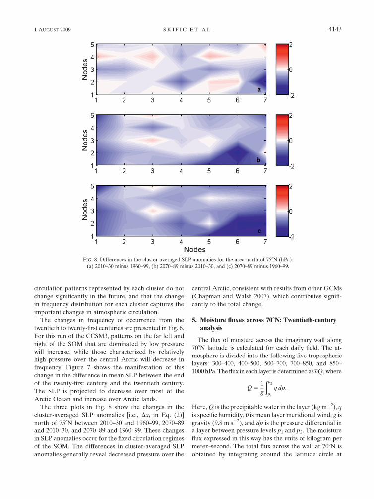
The three plots in Fig. 8 show the changes in the

cluster-averaged SLP anomalies [i.e., Dxi in Eq. (2)]

north of 758N between 2010–30 and 1960–99, 2070–89

and 2010–30, and 2070–89 and 1960–99. These changes

in SLP anomalies occur for the fixed circulation regimes

of the SOM. The differences in cluster-averaged SLP

anomalies generally reveal decreased pressure over the

central Arctic, consistent with results from other GCMs

(Chapman and Walsh 2007), which contributes signifi-

cantly to the total change.

5. Moisture fluxes across 708N: Twentieth-centuryanalysis

The flux of moisture across the imaginary wall along

708N latitude is calculated for each daily field. The at-

mosphere is divided into the following five tropospheric

layers: 300–400, 400–500, 500–700, 700–850, and 850–

1000 hPa. The flux in each layer is determined as yQ, where

Q 51

g

ðp2

p1

q dp.

Here, Q is the precipitable water in the layer (kg m22), q

is specific humidity, �y is mean layer meridional wind, g is

gravity (9.8 m s22), and dp is the pressure differential in

a layer between pressure levels p1 and p2. The moisture

flux expressed in this way has the units of kilogram per

meter–second. The total flux across the wall at 708N is

obtained by integrating around the latitude circle at

FIG. 8. Differences in the cluster-averaged SLP anomalies for the area north of 758N (hPa):

(a) 2010–30 minus 1960–99, (b) 2070–89 minus 2010–30, and (c) 2070–89 minus 1960–99.

1 AUGUST 2009 S K I F I C E T A L . 4143

each level and multiplying by the latent heat of evapo-

ration (L 5 2.5 3 106 J kg21). The values at each level

are then summed vertically to obtain the total moisture

transport into the Arctic Fq, which has units of watts. It

is common to express this value as a flux per unit area of

the Arctic region, so the flux is divided by the area of the

polar cap north of 708N to obtain units of watts per

square meter.

The twentieth-century mean, zonally averaged mois-

ture flux profile L(yq) across 708N for CCSM3 (blue

line) and ERA-40 (green line) is presented in Fig. 9.

Greenland has been excluded from the calculations. The

model reproduces the observed moisture flux remarkably

well. The largest differences occur in the lower levels,

which results in the model overestimating the twentieth-

century moisture flux across 708N by about 12%. The

larger modeled fluxes in the lower levels are likely re-

lated to the generally lower Arctic SLP in the model than

in ERA-40. Above 850 hPa, however, the model profile is

nearly indistinguishable from the observed values.

Because each day of ERA-40 and model output can

be ascribed to one of the SOM clusters, we can analyze

poleward moisture fluxes corresponding to each atmo-

spheric pattern in the SOM matrix. The cluster-averaged

values of the flux across 708N are presented in Fig. 10

(Greenland has been excluded). Red areas in Fig. 10

correspond to patterns in the master SOM character-

ized by strong Icelandic lows and by pronounced low

pressure over the central Arctic, both of which tend to

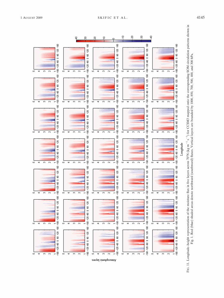
advect large quantities of moisture poleward. Figure 11

presents a height–longitude view of moisture flux across

708N mapped onto the circulation patterns in the master

SOM [kg (m s)21]. The strongest moisture transport

occurs in the lower and the middle troposphere, where

the specific humidity is typically largest. Strong positive

(poleward) moisture fluxes (red shading) are located

east of the low pressure centers and west of the high

pressure regions in the corresponding clusters in the

master SOM. Correspondingly, negative equatorward

moisture fluxes (blue areas) are found west of the low

pressure systems and east of the high pressure features.

Features in the lower-right portion of the SOM generate

the highest moisture transport. These patterns corre-

spond to a positive North Atlantic Oscillation (NAO)

index (Hurrell et al. 2003), with a pronounced Icelandic

low in the Atlantic sector and high pressure over the

Eurasian continent. The circulation patterns in the center

of the SOM, related to weak or moderate high pressure

over the central Arctic, generally show the weakest

northward moisture transport. High pressure over the

central Arctic, usually centered in the Beaufort Sea,

generally indicates divergent flow and a stronger south-

ward branch of moisture transport across the Canadian

Arctic archipelago. Strong, low pressure over the central

Arctic favors convergence and increased northward

moisture transport (patterns in the lower-left corner).

Seasonal-mean moisture fluxes across 708N for the

model’s twentieth century are presented in Fig. 12. Fluxes

are strongest in summer primarily because of the in-

creased depth of the moist layer and generally more

poleward wind vectors (Groves and Francis 2002). A

deeper moist layer also allows the stronger upper-level

winds to advect more moisture during summer. In winter

fluxes are the weakest, because precipitable water values

are lower, and the moist layer is shallow under a strong

surface-based inversion. The strongest fluxes in all seasons

FIG. 9. Vertical profiles of the twentieth-century mean, zonally

averaged latent heat flux across 708N (J kg21 m s21) from CCSM3

(blue line) and ERA-40 (green line).FIG. 10. Cluster-averaged moisture flux across 708N (W m22) from

CCSM3 during 1960–99.

4144 J O U R N A L O F C L I M A T E VOLUME 22

FIG

.1

1.

Lo

ng

itu

de

–h

eig

ht

rep

rese

nta

tio

no

fth

em

ois

ture

flu

xin

fiv

ela

yers

acr

oss

708N

(kg

m2

1s2

1)

for

CC

SM

3m

ap

pe

do

nto

the

corr

esp

on

din

gS

OM

circ

ula

tio

np

att

ern

ssh

ow

nin

Fig

.1

.R

ed

(blu

e)

sha

de

da

reas

de

no

ten

ort

hw

ard

(so

uth

wa

rd)

flu

xe

s.V

ert

ica

lla

yers

are

bo

un

de

db

y1

00

0,

85

0,

70

0,

50

0,

40

0,

an

d3

00

hP

a.

1 AUGUST 2009 S K I F I C E T A L . 4145

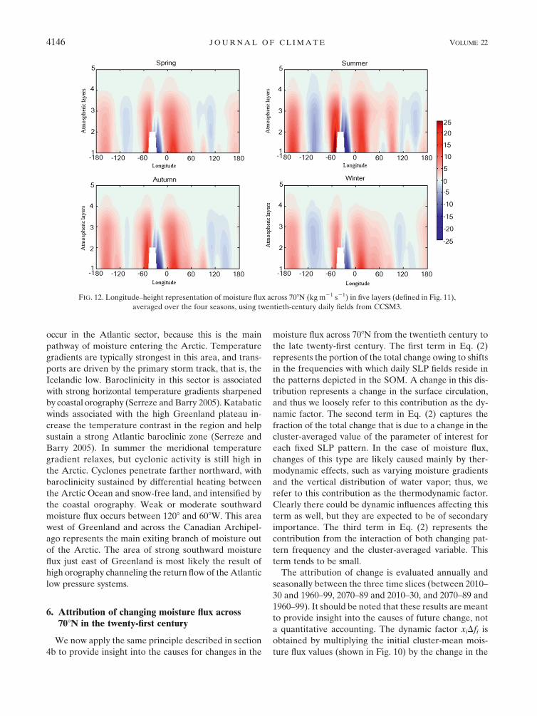
occur in the Atlantic sector, because this is the main

pathway of moisture entering the Arctic. Temperature

gradients are typically strongest in this area, and trans-

ports are driven by the primary storm track, that is, the

Icelandic low. Baroclinicity in this sector is associated

with strong horizontal temperature gradients sharpened

by coastal orography (Serreze and Barry 2005). Katabatic

winds associated with the high Greenland plateau in-

crease the temperature contrast in the region and help

sustain a strong Atlantic baroclinic zone (Serreze and

Barry 2005). In summer the meridional temperature

gradient relaxes, but cyclonic activity is still high in

the Arctic. Cyclones penetrate farther northward, with

baroclinicity sustained by differential heating between

the Arctic Ocean and snow-free land, and intensified by

the coastal orography. Weak or moderate southward

moisture flux occurs between 1208 and 608W. This area

west of Greenland and across the Canadian Archipel-

ago represents the main exiting branch of moisture out

of the Arctic. The area of strong southward moisture

flux just east of Greenland is most likely the result of

high orography channeling the return flow of the Atlantic

low pressure systems.

6. Attribution of changing moisture flux across708N in the twenty-first century

We now apply the same principle described in section

4b to provide insight into the causes for changes in the

moisture flux across 708N from the twentieth century to

the late twenty-first century. The first term in Eq. (2)

represents the portion of the total change owing to shifts

in the frequencies with which daily SLP fields reside in

the patterns depicted in the SOM. A change in this dis-

tribution represents a change in the surface circulation,

and thus we loosely refer to this contribution as the dy-

namic factor. The second term in Eq. (2) captures the

fraction of the total change that is due to a change in the

cluster-averaged value of the parameter of interest for

each fixed SLP pattern. In the case of moisture flux,

changes of this type are likely caused mainly by ther-

modynamic effects, such as varying moisture gradients

and the vertical distribution of water vapor; thus, we

refer to this contribution as the thermodynamic factor.

Clearly there could be dynamic influences affecting this

term as well, but they are expected to be of secondary

importance. The third term in Eq. (2) represents the

contribution from the interaction of both changing pat-

tern frequency and the cluster-averaged variable. This

term tends to be small.

The attribution of change is evaluated annually and

seasonally between the three time slices (between 2010–

30 and 1960–99, 2070–89 and 2010–30, and 2070–89 and

1960–99). It should be noted that these results are meant

to provide insight into the causes of future change, not

a quantitative accounting. The dynamic factor xiDfi is

obtained by multiplying the initial cluster-mean mois-

ture flux values (shown in Fig. 10) by the change in the

FIG. 12. Longitude–height representation of moisture flux across 708N (kg m21 s21) in five layers (defined in Fig. 11),

averaged over the four seasons, using twentieth-century daily fields from CCSM3.

4146 J O U R N A L O F C L I M A T E VOLUME 22

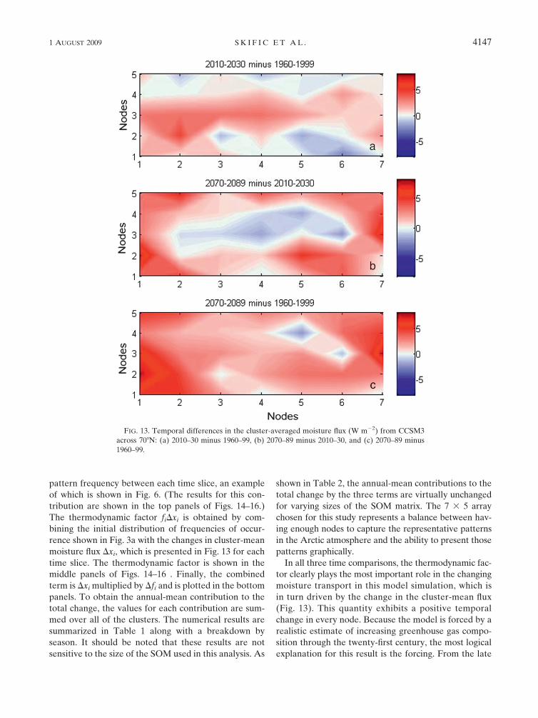
pattern frequency between each time slice, an example

of which is shown in Fig. 6. (The results for this con-

tribution are shown in the top panels of Figs. 14–16.)

The thermodynamic factor fiDxi is obtained by com-

bining the initial distribution of frequencies of occur-

rence shown in Fig. 3a with the changes in cluster-mean

moisture flux Dxi, which is presented in Fig. 13 for each

time slice. The thermodynamic factor is shown in the

middle panels of Figs. 14–16 . Finally, the combined

term is Dxi multiplied by Dfi and is plotted in the bottom

panels. To obtain the annual-mean contribution to the

total change, the values for each contribution are sum-

med over all of the clusters. The numerical results are

summarized in Table 1 along with a breakdown by

season. It should be noted that these results are not

sensitive to the size of the SOM used in this analysis. As

shown in Table 2, the annual-mean contributions to the

total change by the three terms are virtually unchanged

for varying sizes of the SOM matrix. The 7 3 5 array

chosen for this study represents a balance between hav-

ing enough nodes to capture the representative patterns

in the Arctic atmosphere and the ability to present those

patterns graphically.

In all three time comparisons, the thermodynamic fac-

tor clearly plays the most important role in the changing

moisture transport in this model simulation, which is

in turn driven by the change in the cluster-mean flux

(Fig. 13). This quantity exhibits a positive temporal

change in every node. Because the model is forced by a

realistic estimate of increasing greenhouse gas compo-

sition through the twenty-first century, the most logical

explanation for this result is the forcing. From the late

FIG. 13. Temporal differences in the cluster-averaged moisture flux (W m22) from CCSM3

across 708N: (a) 2010–30 minus 1960–99, (b) 2070–89 minus 2010–30, and (c) 2070–89 minus

1960–99.

1 AUGUST 2009 S K I F I C E T A L . 4147

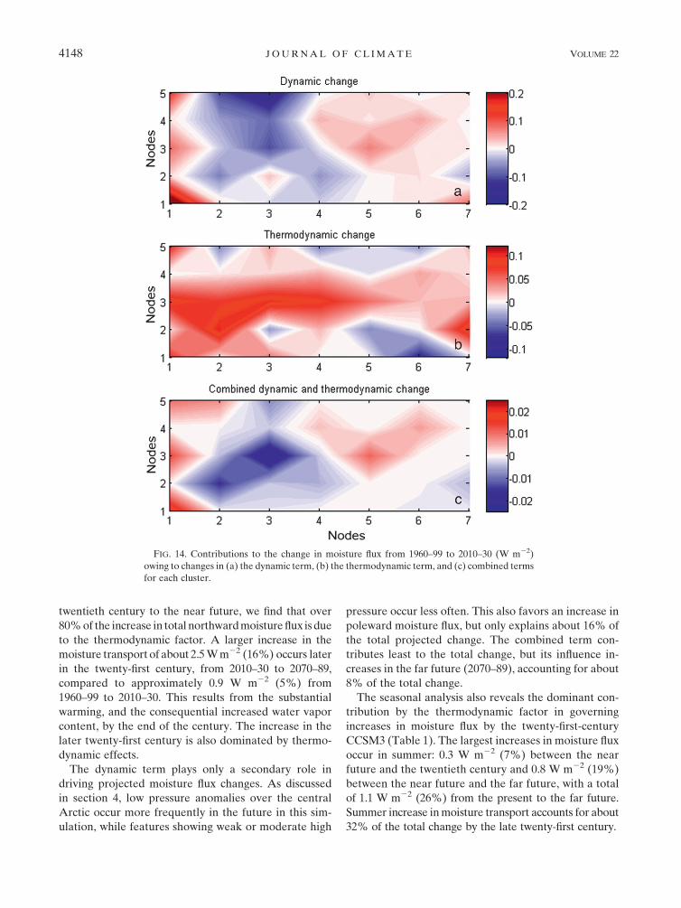
twentieth century to the near future, we find that over

80% of the increase in total northward moisture flux is due

to the thermodynamic factor. A larger increase in the

moisture transport of about 2.5 W m22 (16%) occurs later

in the twenty-first century, from 2010–30 to 2070–89,

compared to approximately 0.9 W m22 (5%) from

1960–99 to 2010–30. This results from the substantial

warming, and the consequential increased water vapor

content, by the end of the century. The increase in the

later twenty-first century is also dominated by thermo-

dynamic effects.

The dynamic term plays only a secondary role in

driving projected moisture flux changes. As discussed

in section 4, low pressure anomalies over the central

Arctic occur more frequently in the future in this sim-

ulation, while features showing weak or moderate high

pressure occur less often. This also favors an increase in

poleward moisture flux, but only explains about 16% of

the total projected change. The combined term con-

tributes least to the total change, but its influence in-

creases in the far future (2070–89), accounting for about

8% of the total change.

The seasonal analysis also reveals the dominant con-

tribution by the thermodynamic factor in governing

increases in moisture flux by the twenty-first-century

CCSM3 (Table 1). The largest increases in moisture flux

occur in summer: 0.3 W m22 (7%) between the near

future and the twentieth century and 0.8 W m22 (19%)

between the near future and the far future, with a total

of 1.1 W m22 (26%) from the present to the far future.

Summer increase in moisture transport accounts for about

32% of the total change by the late twenty-first century.

FIG. 14. Contributions to the change in moisture flux from 1960–99 to 2010–30 (W m22)

owing to changes in (a) the dynamic term, (b) the thermodynamic term, and (c) combined terms

for each cluster.

4148 J O U R N A L O F C L I M A T E VOLUME 22

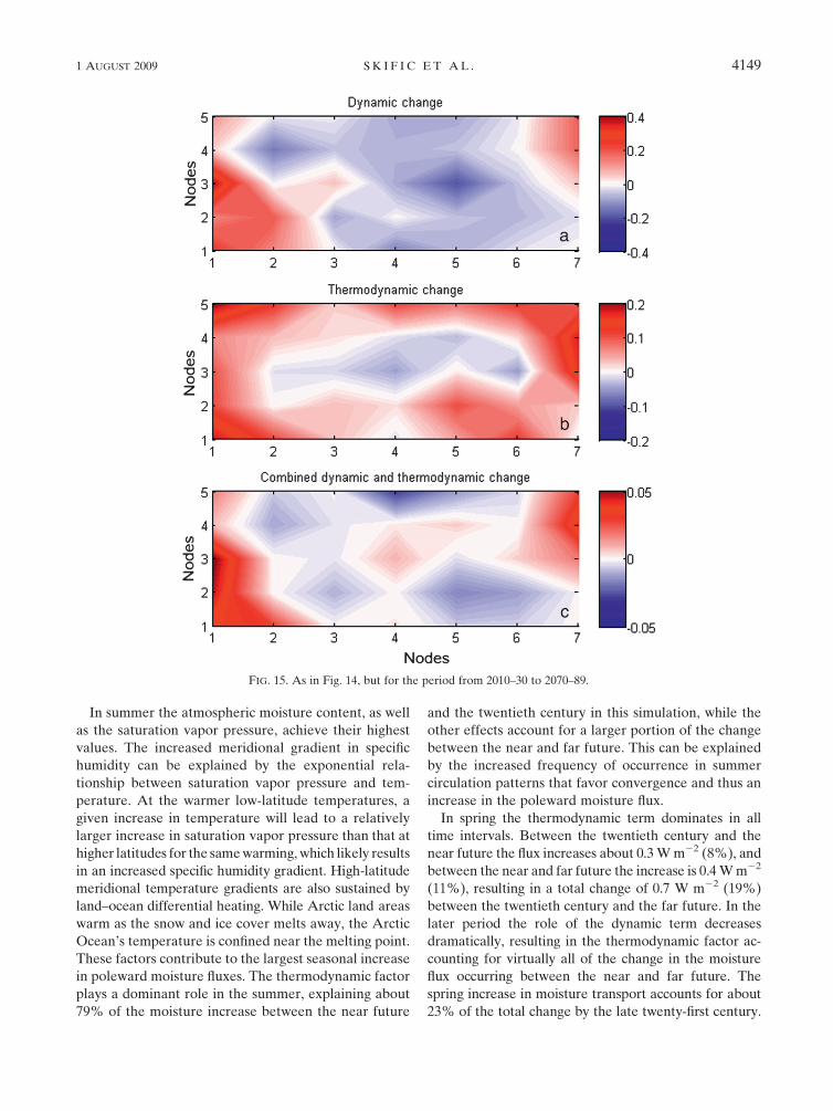
In summer the atmospheric moisture content, as well

as the saturation vapor pressure, achieve their highest

values. The increased meridional gradient in specific

humidity can be explained by the exponential rela-

tionship between saturation vapor pressure and tem-

perature. At the warmer low-latitude temperatures, a

given increase in temperature will lead to a relatively

larger increase in saturation vapor pressure than that at

higher latitudes for the same warming, which likely results

in an increased specific humidity gradient. High-latitude

meridional temperature gradients are also sustained by

land–ocean differential heating. While Arctic land areas

warm as the snow and ice cover melts away, the Arctic

Ocean’s temperature is confined near the melting point.

These factors contribute to the largest seasonal increase

in poleward moisture fluxes. The thermodynamic factor

plays a dominant role in the summer, explaining about

79% of the moisture increase between the near future

and the twentieth century in this simulation, while the

other effects account for a larger portion of the change

between the near and far future. This can be explained

by the increased frequency of occurrence in summer

circulation patterns that favor convergence and thus an

increase in the poleward moisture flux.

In spring the thermodynamic term dominates in all

time intervals. Between the twentieth century and the

near future the flux increases about 0.3 W m22 (8%), and

between the near and far future the increase is 0.4 W m22

(11%), resulting in a total change of 0.7 W m22 (19%)

between the twentieth century and the far future. In the

later period the role of the dynamic term decreases

dramatically, resulting in the thermodynamic factor ac-

counting for virtually all of the change in the moisture

flux occurring between the near and far future. The

spring increase in moisture transport accounts for about

23% of the total change by the late twenty-first century.

FIG. 15. As in Fig. 14, but for the period from 2010–30 to 2070–89.

1 AUGUST 2009 S K I F I C E T A L . 4149

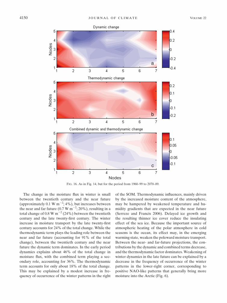
The change in the moisture flux in winter is small

between the twentieth century and the near future

(approximately 0.1 W m22; 4%), but increases between

the near and far future (0.7 W m22; 20%), resulting in a

total change of 0.8 W m22 (24%) between the twentieth

century and the late twenty-first century. The winter

increase in moisture transport by the late twenty-first

century accounts for 24% of the total change. While the

thermodynamic term plays the leading role between the

near and far future (accounting for 91% of the total

change), between the twentieth century and the near

future the dynamic term dominates. In the early period

dynamics explains about 46% of the total change in

moisture flux, with the combined term playing a sec-

ondary role, accounting for 36%. The thermodynamic

term accounts for only about 18% of the total change.

This may be explained by a modest increase in fre-

quency of occurrence of the winter patterns in the right

of the SOM. Thermodynamic influences, mainly driven

by the increased moisture content of the atmosphere,

may be hampered by weakened temperature and hu-

midity gradients that are expected in the near future

(Serreze and Francis 2006). Delayed ice growth and

the resulting thinner ice cover reduce the insulating

effect of the sea ice. Because the important source of

atmospheric heating of the polar atmosphere in cold

seasons is the ocean, its effect may, in the emerging

warming state, weaken the poleward moisture transport.

Between the near- and far-future projections, the con-

tributions by the dynamic and combined terms decrease,

and the thermodynamic factor dominates. Weakening of

winter dynamics in the late future can be explained by a

decrease in the frequency of occurrence of the winter

patterns in the lower-right corner, corresponding to

positive NAO-like patterns that generally bring more

moisture into the Arctic (Fig. 6).

FIG. 16. As in Fig. 14, but for the period from 1960–99 to 2070–89.

4150 J O U R N A L O F C L I M A T E VOLUME 22

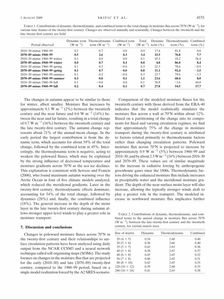
The changes in autumn appear to be similar to those

for winter, albeit smaller. Moisture flux increases by

approximately 0.1 W m22 (2%) between the twentieth

century and the near future and 0.6 W m22 (14%) be-

tween the near and far future, resulting in a total change

of 0.7 W m22 (16%) between the twentieth century and

the late twenty-first century. The autumn change rep-

resents about 21% of the annual-mean change. In the

early period the largest contribution is from the dy-

namic term, which accounts for about 59% of the total

change, followed by the combined term at 45%. Inter-

estingly, the thermodynamic term is negative, acting to

weaken the poleward fluxes, which may be explained

by the strong influence of decreased temperature and

moisture gradients across 708N as the sea ice declines.

This explanation is consistent with Serreze and Francis

(2006), who found maximum autumn warming over the

Arctic Ocean in four of five climate models analyzed,

which reduced the meridional gradients. Later in the

twenty-first century, thermodynamic effects dominate,

accounting for 54% of the total change, followed by

dynamics (28%) and, finally, the combined influence

(18%). The general increase in the depth of the moist

layer in the late twenty-first century during autumn al-

lows stronger upper-level winds to play a greater role in

moisture transport.

7. Discussion and conclusions

Changes in poleward moisture fluxes across 708N in

the twenty-first century and their relationships to sur-

face circulation patterns have been analyzed using daily

output from the NCAR CCSM3 and a neural network

technique called self-organizing maps (SOMs). The study

focuses on changes in the moisture flux that are projected

for the early (2010–30) and late (2070–89) twenty-first

century, compared to the 1960–99 period, based on a

single model realization forced by the A2 SRES scenario.

Comparison of the modeled moisture fluxes for the

twentieth century with those derived from the ERA-40

indicates that the model realistically simulates the

moisture flux across a wall at 708N within about 12%.

Based on a partitioning of the change into its compo-

nents for fixed and varying circulation regimes, we find

that approximately 75% of the change in moisture

transport during the twenty-first century is attributed

to factors related primarily to thermodynamic factors

rather than changing circulation patterns. Poleward

moisture flux across 708N is projected to increase by

approximately 0.9 W m22 (5%) between 1960–99 and

2010–30, and by about 2.5 W m22 (16%) between 2010–30

and 2070–89. These values are of similar magnitude

to the increase in radiative forcing by anthropogenic

greenhouse gases since the 1800s. Thermodynamic fac-

tors driving the enhanced moisture flux include increases

in precipitable water and the meridional moisture gra-

dient. The depth of the near-surface moist layer will also

increase, allowing the typically stronger winds aloft to

play a greater role in the transport. The modeled in-

crease in northward moisture flux implicates further

TABLE 1. Contributions of dynamic, thermodynamic, and combined terms to the total change in moisture flux across 708N (W m22), for

various time frames of the twenty-first century. Changes are observed annually and seasonally. Changes between the twentieth and the

late twenty-first century are bold.

Period observed

Dynamic term

(W m22)

Thermodynamic

term (W m22)

Combined term

(W m22)

Total

(W m22)

Dynamic

term (%)

Thermodynamic

term (%)

Combined

term (%)

2010–30 minus 1960–99 0.2 0.7 0.0 0.9 17.4 81.8 0.8

2070–89 minus 1960–99 0.5 2.6 0.3 3.4 15.5 76.8 7.72010–30 minus 1960–99 winter 0.1 0.0 0.0 0.1 45.5 18.2 36.4

2070–89 minus 1960–99 winter 0.0 0.7 0.1 0.8 4.8 86.8 8.4

2010–30 minus 1960–99 spring 0.1 0.3 20.0 0.3 22.3 78.6 20.9

2070–89 minus 1960–99 spring 0.1 0.7 20.0 0.8 11.1 92.4 23.52010–30 minus 1960–99 summer 0.1 0.2 20.0 0.3 23.7 79.6 23.3

2070–89 minus 1960–99 summer 0.3 0.8 0.1 1.1 23.6 68.4 8.0

2010–30 minus 1960–99 fall 0.1 20.0 0.0 0.1 58.8 23.6 44.8

2070–89 minus 1960–99 fall 0.2 0.4 0.1 0.7 27.8 54.5 17.7

TABLE 2. Contributions of dynamic, thermodynamic, and com-

bined terms to the annual change in moisture flux across 708N

(W m22), between the late twenty-first century and the twentieth

century, for various matrix sizes.

Size of matrix Dynamic Thermodynamic Combined

20 (4 3 5) 0.34 2.68 0.40

30 (5 3 6) 0.36 2.66 0.40

35 (5 3 7) 0.43 2.63 0.36

40 (5 3 8) 0.38 2.67 0.37

48 (6 3 8) 0.45 2.65 0.32

56 (7 3 8) 0.46 2.65 0.31

80 (8 3 10) 0.42 2.65 0.35

120 (10 3 12) 0.39 2.68 0.35

240 (10 3 24) 0.41 2.63 0.38

1 AUGUST 2009 S K I F I C E T A L . 4151

amplification of Arctic warming, because of the release

of additional latent heat through condensation of water

vapor and the increased emissivity of the atmosphere.

Increased warming may augment the already rapidly

declining permanent Arctic ice stores. The increased

moisture content of the high-latitude atmosphere, par-

ticularly in summer, may also lead to an increase in cloud

cover and precipitation, thus intensifying the hydrologic

cycle. Skific et al. (2009) finds that for the same model

simulation, Arctic net precipitation increases by about

20% and mean cloud fraction by about 10% by the late

twenty-first century. They also find that the largest in-

crease in net precipitation over the Arctic Ocean occurs

in summer, with thermodynamic factors accounting for

over 70% of the increase. The summer maximum in

net precipitation is related to a seasonal maximum in

moisture flux convergence (Serreze and Barry 2005),

and thus an increase in moisture flux in the future will

likely lead to increased precipitation in the Arctic. This

eventuality was demonstrated by Cassano et al. (2007),

who find increases in high-latitude precipitation during

the twenty-first century in ensemble output from 15 GCMs

used for the IPCC AR4. They also calculate that more than

75% of that change is due to atmospheric thermodynam-

ics. According to Liu et al. (2007) the increase in winter

moisture transport during the past few decades appears to

be linked with more frequent cyclones and increased

cloud amount in the Arctic.

Our results indicate that moisture fluxes are projected

to increase in this model simulation. The future behav-

ior of the other two components of the moist static en-

ergy flux—geopotential and sensible heat advection—are

yet to be explored in terms of their behavior relative to

moisture transport, their drivers and feedbacks within

the Arctic system, and their roles in Arctic amplifica-

tion. Linkages between the dramatic changes within the

Arctic and the global system remain poorly understood

in present conditions, and thus the uncertainty regard-

ing future changes will remain an important focus for

global change research.

Acknowledgments. We acknowledge and appreciate

the technical support of Gary Strand from the National

Center for Atmospheric Research for providing the

CCSM3 daily outputs used in this study. We are grateful

for the very constructive suggestions by the anonymous

reviewers. Comments and valuable technical informa-

tion was also provided by Eli Hunter from the De-

partment of Marine and Coastal Sciences at Rutgers.

Special thanks go to Jaakko Peltonen of the Depart-

ment of Computer and Information Science at Helsinki

University of Technology, for his helpful advice in ap-

plying the self-organizing maps algorithm. This work is

funded by the National Science Foundation, NSF ARC-

0455262 and ARC-0629412.

REFERENCES

Alexeev, V. A., P. L. Langen, and J. R. Bates, 2005: Polar ampli-

fication of surface warming on an aquaplanet in ‘‘ghost forc-

ing’’ experiments without sea ice feedbacks. Climate Dyn., 24,

655–666.

Ammann, C. M., G. A. Meehl, W. M. Washington, and C. S. Zender,

2003: A monthly and latitudinally varying volcanic forcing

dataset in simulations of 20th century climate. Geophys. Res.

Lett., 30, 1657, doi:10.1029/2003GL016875.

Armstrong, R., M. J. Brodzik, and A. Varani, 1997: The NSIDC

EASE-Grid: Addressing the need for a common, flexible,

mapping and gridding scheme. Earth System Monitor, Vol. 7,

No. 3, 6–7.

Belchansky, G. I., D. C. Douglas, and N. G. Platonov, 2004: Du-

ration of the Arctic sea ice melt season: Regional and inter-

annual variability, 1979–2001. J. Climate, 17, 67–80.

Blanchet, G. E., and J. P. Girard, 1995: Water vapor temperature

feedback in the formation of continental Arctic air: Implica-

tion for climate. Sci. Total Environ., 160/161, 793–802.

Cassano, J. J., P. Uotilla, A. H. Lynch, and E. N. Cassano, 2007:

Predicted changes in synoptic forcing of net precipitation in

large Arctic river basins during the 21st century. J. Geophys.

Res., 112, G04S49, doi:10.1029/2006JG000332.

Cassou, C., and L. Terray, 2001: Dual influence of Atlantic and

Pacific SST anomalies on the North Atlantic/Europe winter

climate. Geophys. Res. Lett., 28, 3195–3198.

Chapman, W. L., and J. E. Walsh, 2007: Simulations of Arctic

temperature and pressure by global coupled models. J. Cli-

mate, 20, 609–632.

Collins, W. D., and Coauthors, 2006: The Community Climate

System Model Version 3 (CCSM3). J. Climate, 19, 2122–2143.

Comiso, J., 2003: Warming trends in the Arctic from clear-sky

satellite observations. J. Climate, 16, 3498–3510.

DeWeaver, E., and C. M. Bitz, 2006: Atmospheric circulation and its

effect on Arctic sea ice in CCSM3 at medium and high reso-

lution. J. Climate, 19, 2415–2436.

Ferguson, D., and Coauthors, 2004: Arctic system synthesis en-

courages program integration. Witness the Arctic, Vol. 11,

No. 1, Arctic Research Consortium of the United States, 8–9.

Fichefet, T., C. Poncin, H. Goose, P. Huybrechts, I. Janssens, and

H. Le Treut, 2003: Implications of changes in freshwater flux

from the Greenland ice sheet for the climate of the 21st cen-

tury. Geophys. Res. Lett., 30, 1911, doi:10.1029/2003GL017826.

Finnis, J., J. Cassano, M. Holland, M. Serreze, and P. Uotila, 2009a:

Synoptically forced hydroclimatology of major Arctic water-

sheds in general circulation models, Part 1: The MacKenzie

River basin. Int. J. Climatol., doi:10.1002/joc.1753, in press.

——, ——, ——, ——, and ——, 2009b: Synoptically forced hy-

droclimatology of major Arctic watersheds in general circu-

lation models, Part 2: Eurasian watersheds. Int. J. Climatol.,

doi:10.1002/joc.1769, in press.

Graversen, R. G., T. Mauritsen, M. Tjernstrom, E. Kallen, and

G. Svennson, 2008: Vertical structure of recent Arctic warming.

Nature, 451, 53–56.

Groves, D. G., and J. A. Francis, 2002: Moisture budget of the

Arctic atmosphere from TOVS satellite data. J. Geophys.

Res., 107, 4391, doi:10.1029/2001JD001191.

Hartmann, D. L., 1994: Global Physical Climatology. Academic

Press, 409 pp.

4152 J O U R N A L O F C L I M A T E VOLUME 22

Held, I. M., and B. J. Soden, 2006: Robust responses of the hy-

drological cycle to global warming. Annu. Rev. Energy En-

viron., 25, 441–475.

Hewitson, B. C., and R. G. Crane, 2002: Self-organizing maps:

Applications to synoptic climatology. Climate Res., 22,

13–26.

Hoerling, M. P., J. W. Hurrell, T. Xu, T. G. Bates, and A. Phyllips,

2004: Twentieth-century North Atlantic climate change. Part II:

Understanding the effect of Indian Ocean warming. Climate

Dyn., 23, 391–405.

Holland, M. M., J. Finnis, and M. C. Serreze, 2007: Simulated

Arctic Ocean freshwater budgets in the twentieth and twenty-

first centuries. J. Climate, 19, 6221–6242.

Huntington, H., and S. Fox, 2005: The changing Arctic: Indigenous

perspectives. The Arctic Climate Impact Assessment (ACIA),

L. Arris, Ed., Cambridge University Press, 61–98.

Hurrell, J. W., Y. Kushnir, G. Ottersen, and M. Visbeck, 2003:

An overview of the North Atlantic Oscillation. The North

Atlantic Oscillation: Climatic Significance and Environmental

Impact, Geophys. Monogr., Vol. 134, Amer. Geophys. Union,

1–36.

——, M. P. Hoerling, and T. Xu, 2004: Twentieth century North

Atlantic climate change. Part I: Assessing determination.

Climate Dyn., 23, 371–389.

Kiehl, J., T. Schneider, R. Portmann, and S. Solomon, 1999: Cli-

mate forcing due to tropospheric and stratospheric ozone.

J. Geophys. Res., 104, 31 239–31 254.

Kohonen, T., 2001: Self-Organizing Maps. 3rd ed. Springer-Verlag,

501 pp.

Lean, J. L., Y.-M. Wang, and N. R. Sheeley Jr., 2002: The effect of

increasing solar activity on the Sun’s total and open magnetic

flux during multiple cycles: Implications for solar forcing of cli-

mate. Geophys. Res. Lett., 29, 2224, doi:10.1029/2002GL015880.

Liu, Y., J. R. Key, J. A. Francis, and X. Wang, 2007: Possible

causes of decreasing cloud cover in the Arctic winter,

1982–2000. Geophys. Res. Lett., 34, L14705, doi:10.1029/

2007GL030042.

Nakamura, N., and A. H. Oort, 1988: Atmospheric heat budgets of

the polar regions. J. Geophys. Res., 93, 9510–9524.

Nakicemovic, N., and R. Swart, 2000: Emission Scenarios. Cam-

bridge University Press, 570 pp.

Osterkamp, T. E., and V. E. Romanovsky, 1999: Evidence for

warming and thawing of discontinuous permafrost in Alaska.

Permafrost Periglacial Processes, 10, 17–37.

Overpeck, J. T., and Coauthors, 2005: Arctic system on trajectory

to new, seasonally ice-free state. Eos, Trans. Amer. Geophys.

Union, 86, 309–313.

Peterson, B. J., R. M. Holmes, J. W. McClelland, C. V. Vorosmarty,

R. B. Lammers, A. I. Shiklomanov, I. A. Shiklomanov, and

S. Rahmstorf, 2002: Increasing river discharge to the Arctic

Ocean. Science, 298, 2171–2173.

Pielke, R., T. Wigley, and C. Green, 2008: Dangerous assumptions.

Nature, 452, 531–532.

Rahmstorf, S., A. Cazenave, J. A. Church, J. A. Hansen, R. F. Keeling,

D. E. Parker, and R. J. Somerville, 2007: Recent climate ob-

servations compared to projections. Science, 316, 709.

Reusch, D. B., R. B. Alley, and B. C. Hewitson, 2005: Relative

performance of self-organizing maps and principal compo-

nent analysis in pattern: Extraction from synthetic climato-

logical data. Polar Geogr., 29, 188–212.

Rigor, I. G., and J. M. Wallace, 2004: Variations in the age of

Arctic sea-ice and summer sea-ice extent. Geophys. Res. Lett.,

31, L09401, doi:10.1029/2004GL019492.

Serreze, M. C., and R. G. Barry, 2005: The Arctic Climate System.

Cambridge University Press, 146 pp.

——, and J. A. Francis, 2006: The Arctic on the fast track of

change. Weather, 61, 65–69.

Skific, N., J. A. Francis, and J. J. Cassano, 2009: Attribution of

seasonal and regional changes in Arctic moisture conver-

gence. J. Climate, in press.

Smith, S. J., and T. M. L. Wigley, 2001: Global and regional an-

thropogenic sulfur dioxide emissions. Global Planet. Change,

29, 99–119.

——, R. Andres, E. Conception, and J. Lurz, 2004: Historical

sulfur dioxide emissions, 1850–2000: Methods and results.

Joint Global Change Research Institute Rep. PNNL-14537,

1–16. [Available online at http://www.pnl.gov/main/publications/

external/technical_reports/PNNL-14537.pdf.]

Soden, B. J., and I. M. Held, 2006: An assessment of climate

feedbacks in coupled ocean–atmosphere models. J. Climate,

19, 3354–3360.

Solomon, S., and Coauthors, 2007: Climate Change 2007: The

Physical Science Basis. Cambridge University Press, 996 pp.

Thompson, D. W. J., and J. M. Wallace, 1998: The Arctic oscilla-

tion signature in the wintertime geopotential height and

temperature fields. Geophys. Res. Lett., 25, 1297–1300.

Uppala, S. M., and Coauthors, 2005: The ERA-40 Reanalysis.

Quart. J. Roy. Meteor. Soc., 131, 2961–3012.

1 AUGUST 2009 S K I F I C E T A L . 4153