Embed Size (px)
Citation preview

AUTOMATED CONFLATION FRAMEWORK FOR INTEGRATING
TRANSPORTATION BIG DATASETS
_______________________________________
A Thesis presented to the faculty of the Graduate School
at the University of Missouri-Columbia
_______________________________________
In Partial Fulfilment
of the Requirements for the Degree
Master of Science in Civil Engineering
_______________________________________
by
Neetu Choubey
Dr. Yaw Adu-Gyamfi, Thesis Supervisor
DECEMBER 2019

The undersigned, appointed by the dean of the Graduate School, have examined the
thesis entitled
AUTOMATED CONFLATION FRAMEWORK FOR INTEGRATING
TRANSPORTATION BIG DATASETS
Presented by Neetu Choubey,
A candidate for the degree of Master of Science,
And hereby certify that, in their opinion, it is worthy of acceptance.
Dr. Yaw Adu-Gyamfi
Dr. Carlos Sun
Dr. Timothy Matisziw

ii
ACKNOWLEDGMENTS
The first person that comes in my mind when I start acknowledging people for their
contribution during my research work is my advisor Dr. Yaw Adu-Gyamfi. His constant
support and guidance have helped immensely to give shape to my work. I always looked
at him and gotten help (absolutely) whenever any challenges baffled me. He has
accommodated my odd working hours and always been gracious and supportive through
his words. He was and will be my major source of learning. Apart from him, I would like
to thank Dr. Praveen Edara who has introduced me to Mizzou and gave this wonderful
opportunity to pursue my higher studies here in Columbia, Missouri.
Secondly, I would like to thank my family who has empowered me during this roller coaster
ride. My mother Jyoti Choubey, my father Ajit Choubey, and my sister Neha Sharma had
given warmth through their words during the cold nights working in the lab. I would also
like to thank my lab mates Nipjyoti, Vishal and Farzaneh for their constant feedback and
being my source of entertainment.
I would also like to thank my thesis committee members, Dr. Sun and Dr. Matisziw for
accommodating my request and spending time on understanding my work and efforts on
giving me their invaluable feedback.
At last but definitely not the least, I would like to thank my fiancée Aniket for being there
for me always.
iii
TABLE OF CONTENTS
ACKNOWLEDGMENTS ................................................................................................ ii
LIST OF FIGURES .......................................................................................................... v
LIST OF TABLES .......................................................................................................... vii
ABSTRACT .................................................................................................................... viii
CHAPTER 1 INTRODUCTION ..................................................................................... 1
1.1 Conflation- An overview ......................................................................................... 2
1.2 Problem Statement ............................................................................................. 5
1.3 Objectives of the study ....................................................................................... 6
CHAPTER 2 LITERATURE REVIEW ......................................................................... 8
CHAPTER 3 PROPOSED METHODOLOGY ........................................................... 13
3.1 INRIX and LRS Conflation .................................................................................. 15
3.1.1 Traditional GIS conflation toolsets ................................................................... 15
3.1.2 Proposed Methodology ...................................................................................... 20
3.2 INRIX and Transit Conflation: ........................................................................... 32
3.3 INRIX and Detector Conflation ........................................................................... 33
3.4 INRIX-Crash ......................................................................................................... 34
CHAPTER 4 RESULTS AND DISCUSSION .............................................................. 36
4.1 Data description: ................................................................................................... 36
The data involved in this research work includes- ................................................... 36

iv
4.2 Conflation Result Discussion ................................................................................ 40
4.3 Challenges with the current results ..................................................................... 50
4.4 Concluding Remarks and Recommendations .................................................... 56
REFERENCES ................................................................................................................ 60

v
LIST OF FIGURES
Figure 1: Conflation- An Overview35 .............................................................................. 4
Figure 2: Adopted Process for conflation ..................................................................... 14
Figure 3: Automated Conflation Process ...................................................................... 15
Figure 4: Traditional Conflation tool flow chart ......................................................... 15
Figure 5: Results of using the DFC tool ........................................................................ 17
Figure 6: ArcGIS Rubbersheet Tool for Feature Matching ....................................... 18
Figure 7: Feature Matching Results for a Selected Road (I-29). ................................ 18
Figure 8: Proposed Methodology flow chart ................................................................ 20
Figure 9: INRIX segments before and after the first tier of conflation ..................... 24
Figure 10: Bearing of a line ............................................................................................ 25
Figure 11: Conflation Rate for Interstates ................................................................... 26
Figure 12: LRS and INRIX conflation for Interstates ................................................ 27
Figure 13: Feature matching using bearing ................................................................. 29
Figure 14: Variation of Conflation Rate and Accuracy with respect to the search
radius ................................................................................................................................ 30
Figure 15: INRIX Transit Overlays and Conflation ................................................... 33
Figure 16: INRIX Detector Overlays and Conflation ................................................. 35
Figure 17: INRIX Crash Overlays and Conflation ...................................................... 35
Figure 18: LRS and INRIX road networks .................................................................. 38
Figure 19 Conflation Rate and Accuracy for Interstates. ........................................... 41
Figure 20: Conflation rate and accuracy for bearing .................................................. 42
Figure 21: Travel time interactivity .............................................................................. 45

vi
Figure 22: TITAN Interactive Dashboard for exploring statewide mobility ............ 45
Figure 23:Statewide safety mobility dashboard ........................................................... 46
Figure 24: Overlay of all conflated layers and travel time visualization ................... 48
Figure 25: Variation in the distance between two matching segments ...................... 52
Figure 26:Bearing Conflation for Kansas St ................................................................ 53
Figure 27: Influence of segment length in conflation rate........................................... 54
Figure 28: I-44 from LRS and INRIX layer ................................................................. 56

vii
LIST OF TABLES
Table 1: Transfer Attribute Output Table ................................................................... 19
Table 2: Road name attribute matching results........................................................... 22
Table 3: Direction Combination .................................................................................... 23
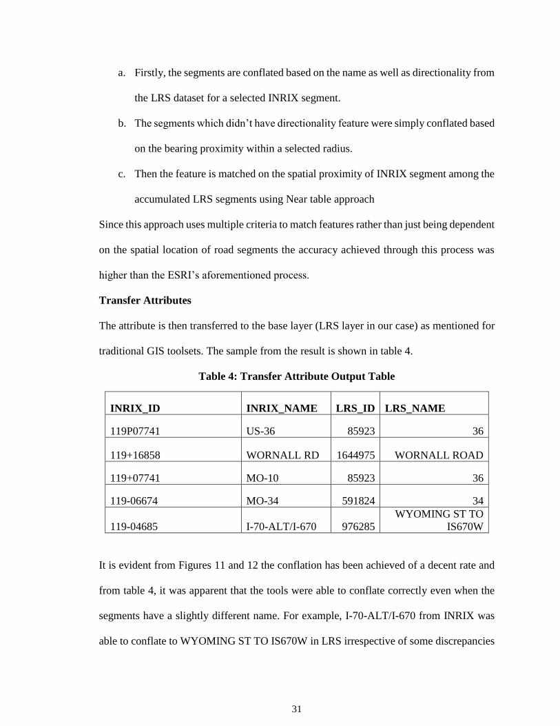
Table 4: Transfer Attribute Output Table ................................................................... 31
Table 5: INRIX data set ................................................................................................. 36
Table 6: LRS data set ..................................................................................................... 37
Table 7: Transit data ...................................................................................................... 38
Table 8: Detector Dataset ............................................................................................... 39
Table 9 Conflation rate and Accuracies for few Major roads .................................... 43
Table 10: Conflation Rates for the various layers ....................................................... 47
Table 11: Final conflated layer ...................................................................................... 48
Table 12: Text name subtleties for certain major roads ............................................. 51

viii
ABSTRACT
The constant merging of the data, commonly known as Conflation, from various sources,
has been a vital part for any phase of development, be it planning, governing the existing
system or to study the effects of any intervention in the system. Conflation allows
enriching the existing data by integrating information through numerous sources
available out there. This process becomes unusually critical because of the complexities
these diverse data bring along such as, distinct accuracies with which data has been
collected, projections, diverse nomenclature adaption, etc., and hence demands special
attention. Although conflation has always been a topic of interest among researchers,
this area has witnessed a significant enthusiasm recently due to current advancements in
the data collection methods. Even though with this escalation in interest, the developed
methods didn’t justify the expansions field of data collections has made. Contemporary
conflation algorithms still lack an efficient automated technique; most of the existing
system demands some sort of human involvement for the analysis to achieve higher
accuracy. Through this work, an effort has been made to establish a fully automated
process to conflate the road segments of Missouri state from two big data sources. Taking
the traditional conflation a step further, this study has also focused on enriching the road
segments with traffic information like delay, volume, route safety, etc., by conflating
with available traffic data and crash data. The accuracy of the conflation rate achieved
through this algorithm was 80-95% for the different data sources. The final conflated layer
gives detailed information about road networks coupled with traffic parameters like delay,
travel time, route safety, travel time reliability, etc.
1
CHAPTER 1 INTRODUCTION
The process of enhancing one dataset with the additional information available in different
forms and formats from various sources has been here since the term ‘data collection’ has
been coined. This process of augmenting information of a source by supplementing data is
known as Conflation. The practice of conflation is not restricted to any particular field,
from subjective fields of psychology, biology to the fields as diverse as transportation
engineering, the use of tools from time to time to enhance the current data sets is prevalent.
In this study, we are using the concept of conflation for the integration of transportation
big data sets from various sources to get a final layer of the road network which will have
supplemented information from all the conflated layers.
The initial practice of conflation was usually achieved by overlaying, intersecting and
cross-referencing of map layers manually to get a final map with all the statistics and
projections from the different map layers. The problem of data inconsistencies both in the
spatial and attribute domains presents obstacles in using data for analysis, overlays, and
mapping. The need for integration of these diverse data has become principally important
with the current advancements in the technology and the ease in the data collection
methods. With the increase in the efficiency of data collection, the size of collected data
has increased exponentially and that’s why the term big data has become a part of various
field’s argot as well. While trading with data it is usual to encounter different geospatial
sources that bring anomalies and heterogeneity along as the nomenclature and accuracy
adopted vary with sources of data. It becomes difficult to identify the same features from

2
distinct data sources due to different ways the data is represented in a different way. These
irregularities can be overcome manually if the size of data is manageable; nevertheless,
this becomes infeasible as soon as data begins to inflate and hence demands some sort of
sophistication in dealings.
Due to all these progressions, the technology has made and dynamic changes in the data
availability and propensity, there is a dire need to find a tool that can automate the process
of the conflation with a higher accuracy that can handle the integration of datasets in such
a big scale.
1.1 Conflation- An overview
Initially, the primary objective of conflation was to eliminate any sort of spatial
inconsistency from the various vector maps to achieve a desirable accuracy. The primary
objective of removing such altitudinal discrepancies was to allow easier transfer of
attributes from one map to another [1]. From there the utilization of conflation has become
quite diverse, from removing discrepancies to adding missing details, it has found uses in
various aspects of data integration. Geographic Information Systems (GIS) is one of the
important fields where conflation plays a vital role mainly due to the size of such files and
it is hard to get all the data from a single source. To do any GIS analysis, there is always a
factor of heterogeneity that needs to be addressed as the GIS data assemblage is pretty
tedious and still expensive to be afforded by a single agency. By default, such kind of data
brings along a large number of inconsistencies among information accumulated from
various sources. In the field of transportation engineering, GIS data plays an important role,
from traffic designs, Intelligent Transportation System (ITS) to transportation planning,
every aspect requires some sort of GIS data analysis. For the different GIS layers, the
3
traditional methods mostly comprise of using Rubbersheet or Align features which take
care of the anomaly inaccuracies, misalignment, etc., among the data; however, their
application is limited, time-consuming and not so satisfactory, especially, when dealing
with transportation big datasets.
Conflation is not only limited to dealing with the same data type, but there are also certain
regions where it requires to find a relation between information belonging to different data
type altogether. For example, the crash data usually comes in an excel or a CSV file
whereas the road data on which these crashes occur come in either GIS or excel/CSV
format, for a better visualization of the fusion of these two data sets, a GIS conflation would
do more justification as compared to a simple excel file merging. The visual representation
of data like a heat map, the color symbolization of road network based on crash type can
be achieved only if the relationship between these different data types/sources can be
established. Because of such atypical requirements, another aspect of conflation which has
started gathering attention is data fusion; the interest in data fusion has become quite
substantial in the recent time mostly due to the need of working with different data type
from various sources. If we see the field of big data, these data comprise of information
collected from many sources and have a completely different data type, even a simple
representation of this data needs coordination and correlation among these data sources
and type.
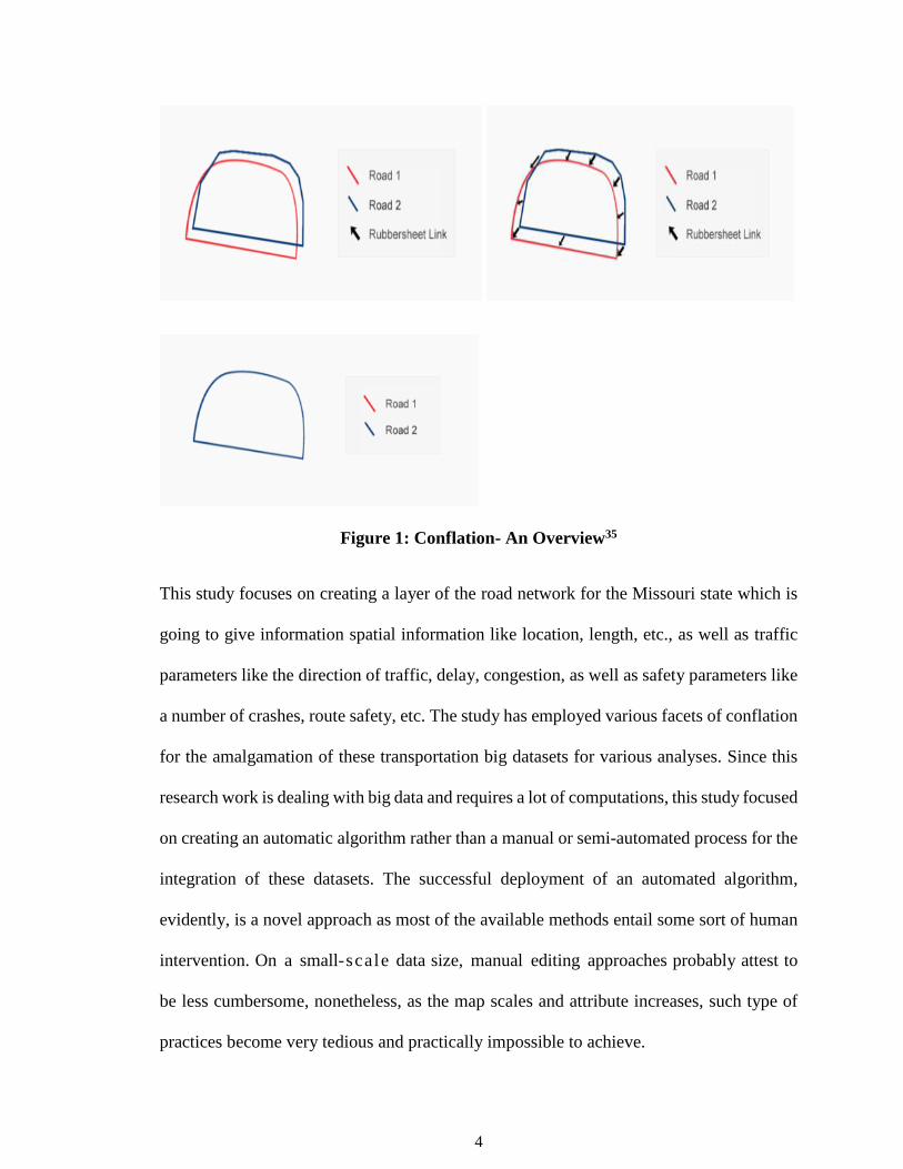
A typical example of the conflation of road networks from two data sets has been shown
in figure 1.
4
Figure 1: Conflation- An Overview35
This study focuses on creating a layer of the road network for the Missouri state which is
going to give information spatial information like location, length, etc., as well as traffic
parameters like the direction of traffic, delay, congestion, as well as safety parameters like
a number of crashes, route safety, etc. The study has employed various facets of conflation
for the amalgamation of these transportation big datasets for various analyses. Since this
research work is dealing with big data and requires a lot of computations, this study focused
on creating an automatic algorithm rather than a manual or semi-automated process for the
integration of these datasets. The successful deployment of an automated algorithm,
evidently, is a novel approach as most of the available methods entail some sort of human
intervention. On a small-scale data size, manual editing approaches probably attest to
be less cumbersome, nonetheless, as the map scales and attribute increases, such type of
practices become very tedious and practically impossible to achieve.

5
For this study, data available from free sources as well as State DOT’s data were used for
the analysis. There were primarily five types of data used to achieve the objective set for
this study and they were viz. MO-DOT Linear Referencing System (LRS) data for road
networks (LRS), INRIX road data, MO-DOT detector data which gives information like
traffic volume on road networks, Missouri road crash data of three years and Saint Louis
transit data which gives real-time location of buses on road network for a week which
would help in the computation of traffic variables like delay, congestion on the road
networks for the Saint Louis County.
1.2 Problem Statement
In the field of transportation engineering, it is quite usual to encounter data of a different
kind and then trying to establish a relation among them to derive some interpretation for
the overall transportation system. The transportation data collection is still a big scale and
an expensive investment, and this is one of the key reasons that it is hard to find data from
a single source. This is simply due to the monetary as well as the human effort which goes
in the collection as well as maintenance of such large data sets. Even among a county, data
collection report varies with the agency to agency and it is hard to form a single
organization dealing with all aspects of one data type. Crash reports for different types of
the accident on roads is a classic case of nomenclature anomalies, hence the application of
conflation is far and wide in transportation engineering. Due to this diverse data type, the
conflation of various data sets is usually achieved by manual methods using tools like
excel; since the transportation data numbers are increasing exponentially, manual methods
found to be expensive, inefficient and sometimes even counterproductive. The proposed
methodology is going to deploy an automated conflation algorithm which not only

6
overcomes the diverse data problem but also eradicates the requirement of manual
conflation by employing data fusion and features alignment through the programming
language as well as the GIS tools for analysis as data chosen for this study comprises of
GIS as well as CSV data. The ready to use tools available in the market were also used for
the comparison of the proposed method and it was found that the automated algorithm
proved to be more accurate and computationally efficient as well. Thus, the proposed tool
is capable of dealing data sets on a big scale as well as overcomes the problem of
heterogeneity with satisfactory accuracy.
1.3 Objectives of the study
The objectives of this study can be summarized in the following points:
• The conflation of diverse data sets: In this study, the tools for the conflation of
multiple layers is to be developed using the theory of overlaying, feature matching
as well as data fusion. The layers matching in this study include:
▪ LRS and INRIX: An algorithm is to be developed to conflate big data sets
of road shapefiles collected from two sources viz. INRIX and MO-DOT.
This tool would aim to develop a final layer with enhanced information
from both datasets by surmounting spatial discrepancies, accuracies, and
differences in nomenclature adoption.
▪ INRIX and Crash data: A tool is proposed here to fuse the data from two
different types of information background using a common linear reference
used on the road network. This procedure would lead to the assignment of
crashes from crash reports to respective road networks.

7
▪ INRIX and Transit data: The third methodology planned to be designed here
would use the concept of data fusion to align the information from different
resources viz. road shapefiles and real-time location of transit system on
road networks, to analyze traffic variables like delay congestion, travel
time, etc., on the county-wide road networks.
• Automation: This study aiming to provide a tool that can handle big data sets with
feasible time consumption as well as provides easier scalability to diversified data type
by automating the whole process of conflation. Another aspect of automation that’s
been targeted through this work is achieving a cost-effective tool with satisfactory
accuracy which would discourage the tedious human intervention altogether.

8
CHAPTER 2 LITERATURE REVIEW
Before getting started with the proposed methodology, a literature review has been done
on the development of Conflation methods using the various theories over the years.
The literature review has helped to understand the growth of this research area and find the
gaps where this process of conflation can be tweaked to justify the improvements
technology has made.
The process of assimilation, as well as the orientation of different forms of data sets, can
be defined using the term. The conflation process can be divided into the following
subtasks: [3]
1. Feature matching: Find a set of conjugate point pairs, termed control point pairs, in
two datasets.
2. Match checking: Detect inaccurate control point pairs from the set of control point
pairs for quality control.
3. Alignment: Use the accurate control points to align the rest of the geospatial objects
(such as points or lines) in both datasets by using the triangulation and rubber-
sheeting techniques.
4. Data Fusion: The integration of data from numerous sources to get a final data set
which will have combined information for a better understanding of the
information.
Conflation found its first application around the mid-1930s but the research work in this
field was really sparse; it was only in the late 1980s that this area has gained popularity
among researchers mainly due to the advancements in technology which has made various
9
kinds of data easily available. With the increase in data collection and growth of the
internet, there was an increased interest in working with data to get a fair chance to prove
the researcher’s own interpretations. The development of this tool over the years can be
better understood in the following paragraphs.
The conflation of road segments has been gathering its due interest since the 1980s [1].
A lot of effort has been put afterward [2][3][4]. The research work on conflation started
with very basic intention of improving the existing maps with information available in
different forms and different sources. The methods adopted during 1980 were mainly
focused on making this process as much as automated as possible. With the use of Rubber
sheets in [1] [4] computer recognizes matches between different maps using mathematical
algorithms and graphical positions to detect similarity [4]. During initial times the
methodologies were mainly inspired by statistical methods like proximity of locations
and geometry [5]. Rather than considering conflation as a single method, it has been
considered this as a multistep iterative process namely, positional re-alignment of
component maps, identification of matching features and positional and attribute
deconfliction of positively identified feature matches [5]. In [6] this work has talked about
transferring attributes from one layer to another or adding missing features. Previously
geospatial databases (GDBs) played an important role in accumulating information from
heterogeneous sources [7]. The work like [8],[9],[10] presented studies to justify the need
for merging information from the database with different forms and density, with varied
precision values. In [11], Spatial Data Infrastructure has been adopted to make a
framework that would allow the data interchange between different systems. Works like
[12],[13],[14] talked about data fusion, a traditional method, for the integration of two
10
layers and getting a third layer with supplemented information from both the layers.
These works were particularly famous in the field of remote sensing and GIS [15].
According to [16], even though the conflation term finds its roots in the 1980s, it didn’t see
much of the development until the mid-2000s. The work of the 1980s mainly witnessed the
work of gathering images and maps, development of computational methods based on
graphics and geometry. The conflation method has been primarily dependent on the
feature matching be it a line to line (road to road), polygon to the line (buildings to the
road), point to the line (position to the road), etc. The aforementioned features are known
as geo-objects and determination of relations between these features is known as matching
[17]. Earlier studies have based their work on the above principal like matching of geo-
objects to achieve a conflation [2], [4], [5], [6]. With the advancement in
computational methods, the conflation methods became much more detailed and rather
than adapting generalized feature matching like proximity and feature it became subtler
with the intention of higher accuracy. The methods like distance, angle, buffer growing,
etc. had taken a matching process of data from various sources to a higher level [17].
There have been extensive studies on matching features like roads or buildings commonly
known as polygon conflation [18], [19], [20] to make the traditional maps more
informative. The work in [5], [7], [21], [22], [23], [24] had underlined the significance
of over-lapping important geometric structures like intersections, roundabouts, etc., these
works had used this important location like geometric infrastructures on-road segments
for conflation and coined methods based on this principle. After the successful
implementation of this theory, it became quite popular among researchers and had been a
part of the coming conflation methods, meanwhile, features like Linear and

11
Topographical matching had seen a boost among researchers too. With this achievement
of higher accuracy, now the focus of the researchers shifted from accuracy to automating
this process, especially for handling data on a large scale. Works like [26], [27], [28] had
focused their attention on automating this process as well as achieving higher accuracy. In
[29] the cynosure of this work had been automating the procedure in a semi-automated way.
This work had utilized cluster matching algorithms to find a strong connection between
nodes, edges, and segments; the interactive procedure, on the other hand, allows a user
to rectify the mismatched features which were missed by an automated mechanism. This
approach was a breakthrough in automating the conflation process; however, user
intervention was still a complex way to achieve
reliable results. The work of others like [30], [31] used their works for the specific type
of road patterns rather than focusing on being generic and hence the scalability of these
methods decreased significantly for other types of road segments. Based on the literature
review for this work, it is evident that there is still a good scope for a robust automated
conflation algorithm which can help in achieving higher accuracy, with no user
interference, whatsoever, and still has the scalability to be adapted for all the types
of road segments. There was little to no work seem to be done to inculcate the traffic
aspect of road segments in the map as this was mostly done manually and due to the
size and complexities of this data, it was usually preferred to confine it for an area of
interest itself. This project has focused on taking conflation methods from just improving
spatial data quality to providing more road-specific information like traffic, safety, etc.
This paper has been arranged as follows: Section 3 will be talking about the methodologies
adopted for this procedure. From data preparation to conflation time, the information

12
regarding each step of this algorithm has been discussed here. Section 4 talks about the
results and discussion regarding the outcomes from the conflation. And at last, Section 5
talks about the key take away from this work and the future work which can be done to
make this procedure more efficient in the field of conflation.

13
CHAPTER 3 PROPOSED METHODOLOGY
The methodology developed for automating conflation of the LRS and INRIX datasets and
extended to other datasets includes four key steps: Data pre-processing which prepares the
two geographic data layers in the best condition for further analysis. Next, ESRIs ArcGIS
tools such as “Detect Feature Change” are used to detect spatial and geometric changes in
both datasets. For segments where no change is observed, a one – to – one mapping is
carried out. If there was a spatial change, features are matched based on proximity,
topology, and pattern and similarity analysis. Finally, specific feature attributes from the
source layer are transferred to the matching target features to generate an output
crosswalk table. The overall conflation rate achieved is approximately 95%. The conflated
road segments from LRS and INRIX are then further improved with some real-time traffic
data by conflating time position of transit data, detectors in the roads, and crash data
collected for the Missouri state. Transit data consist of the real-time position of buses
with the timestamp and trip details congregated for a selected county for two consecutive
weeks and were conflated with INRIX road segments. Using the combined information of
INRIX’s average travel time on road segments and travel time gathered from transit data,
the traffic variable delay was calculated; the output of this traffic data viz, delay employed
for interpreting the traffic flow of the route. This understanding of flow was achieved by
conflating another set of traffic layer collected from the detectors placed in various
highways. The detector data brought the important variable traffic count to the existing
map. This spatially joined data with vehicle count and delay helped to comprehend reasons
for the delay such as, whether it is controlled or uncontrolled one. The amalgamation
of crash data with INRIX, on the other hand, helped to give an idea about the safety issues

14
of the state roads, overall. Crash data is the crash report on the various roads on Missouri
noted with respect to mile marker with all the details regarding accident and surroundings
and this mile marker was used as cross-reference while achieving the conflation. This
experiment with the conflation of data from various GIS sources as well as real traffic
data not only gave a map with enhanced spatial information but was also successful in
giving a richer picture of traffic-related queries like travel time, delay and safety of the
roads.
Figure 2: Adopted Process for conflation
Conflation
Data
INRIX
Roa Networks with enriched road information
Gives
LRS
GIS Conflation
INRIX
Road Networks with Traffic
Volume
Gives
Detector
GIS Conflation
INRIX
Road Networks with Safety details
Gives
Crash
Data Fusion
INRIX
GIS Conflation
Road Network with Traffic flow parameters
Gives
Transit
15
3.1 INRIX and LRS Conflation
3.1.1 Traditional GIS conflation toolsets
Figure 4: Traditional Conflation tool flow chart
Data Pre-Processing and Attribute Matching.
This step prepares the data for the best condition possible for further analysis. The two
geographic data layers are collected from two separate vendors. As a result, the potential
for geometric and attribute data inconsistencies is high. The pre-processing stage includes
validating data geometry and topology, selecting relevant attribute features (e.g. road
names, segment ids, counties, etc.) for processing and using consistent map projections to
ensure that the two data layers are projected on the same geographic coordinate system.
Next, attributes in both datasets describing the same features are matched.
Attribute matching feature wasn’t found in the available conflation toolsets and due to this,
there is a high rate of mis conflation i.e., one feature matching to a different segment in
different data sets. Through this proposed method, the matching criterion has been fixed to
•Data proceesed and filtered.
•Attribute matching feature was missing
Data Preprocessing and Attribute
matching
•Use of DFC tool
Feature Cahnge Detection •Based on one
criterion of spatial proximity
Feature Matching Rubbersheet
•Matched feature are tranferred
Attribute Transfer

16
overcome the issue of false conflation and make the process more viable and efficient.
Accuracy: Because the conflation process relies on spatial proximity, a road segment A,
in one layer could be conflated to two road segments, B and C, in another layer although
the bearing (direction of traffic in this context) of either B or C might be opposite to the
bearing of A.
For the GIS conflation tool since there is no tool to match the features, the traditional
conflation toolsets use the proximity measure as only matching criterion which leads to
conflation error. That is, the possibility of matching one INRIX layer to the LRS segment
would completely be dependent on the distance between these two features.
Detect Feature Changes
Feature change detection is the first step in the implementation of the conflation process.
Knowing where and what the changes are between the two datasets helps you assess how
significant they are and whether or not you need to proceed with attribute transfer.
To detect feature changes in both datasets, the DFC tool in ESRIs ArcGIS was used. This
tool identifies spatial feature differences and outputs the type of change detected for each
feature. Ideally, there are four (4) possible changes that could occur:
o Spatial Change (topological difference)
o Attribute Change
o No Change (1:1 match without any spatial or attribute changes)
o New feature (unmatched feature).
Figure 5 shows the results of using the DFC tool to detect feature changes in a selected
region on both datasets. For features where a spatial change was detected, the following
workflows will be used to unify and consequently conflated into the base data which is the

17
LRS in this case.
Figure 5: Results of using the DFC tool
Feature Matching
The goal of feature matching is to map features in the source datasets (INRIX layer) which
experienced a spatial change to its corresponding target features (LRS layer).
For the traditional conflation tool - For the sake of comparison, ESRI’s ArcGIS feature
matching tools were used in this project. These tools match distorted features based on
proximity, topology pattern and similarity analysis, and other optional attributes. An output
of this step is a table storing match information.
The specific tool used in the current study is the “Generate Rubbersheet Tool” shown in
figure 6. This tool generates links between matched features or points where the source and
target locations are identical. Figure 7 shows the results of using the rubbersheet tool to
match INRIX and LRS segments on Interstate 29 East (I-29E). A total of 352 (representing
91%) unique INRIX segments were accurately matched to their corresponding LRS

18
segments. The gaps in the rubbersheet results frame (green layer) shown in figure 7 (part
b) represent regions where road segments were not mapped. The conflation rate does
fluctuate depending on the type, geometry, and length of the road segment. The overall
conflation rate for all road segments will be evaluated in the results section.
Figure 6: ArcGIS Rubbersheet Tool for Feature Matching
Figure 7: Feature Matching Results for a Selected Road (I-29).
50

19
Transfer Attributes
Finally, once features between the two geographic data layers have been matched, specific
feature attributes from the source layer are transferred to the matching target features. Table
1 shows an example transfer attribute output table.
Table 1: Transfer Attribute Output Table
INRIX_ID
LRS_I
D INRIX_NAME LRS_NAME
119-16706 189028 12TH ST 12TH ST
119-19151 346042 18TH ST 18TH ST
119+14152 198748 31ST ST WYANDOTTE ST
119-19041 346313 4TH ST 4TH ST
119N1674
1 186825 6TH ST CHARLOTTE ST
119N1674
1 186686 6TH ST 6TH ST
119+13415 296790 AIRPORT RD AIRPORT RD
119P13415 297903 AIRPORT RD 170
The traditional tool not only lacks the sophistication tools required to deal with diverse data
but also computational infeasible while dealing with big data sets like the road networks
used here. From table 1 it is evident that there was mis conflation, for example, airport road
is conflated to 170 and 31st Street is conflated to WYANDOTTE ST. Since the criterion of
matching was only based on the proximity, this tool fails to encompass the data
inconsistency and assortment.
The approach designed for this study tries to overcome the main drawbacks of existing
tools and modify the conflation process to encompass such anomalies. The process is
discussed in detail in the following section.
20
3.1.2 Proposed Methodology
The proposed methodology uses the same four steps of conflation as its basic criterion,
the flow of this methodology is shown in figure 8. The following subsections would
discuss each step-in detail for the adopted approach here.
Figure 8: Proposed Methodology flow chart
To make sure the process is fully automated python language is used for coding using
various libraries. Most of the functions were defined as per the requirement for this
algorithm, and some famous libraries like pandas, arcpy, numpy, os to achieve the
following steps using python language. The steps of basic conflation are tweaked to address
these irregularities in the datasets.
Data Processing and Attribute Matching
The data preprocessing filtering is pretty much the same as explained for traditional GIS
toolsets.
Attribute Matching: For the attribute matching, the matching feature has been designed
•Data proceesed and filtered.
Data Preprocessing
•Attibute matching using the feature
county, road name and traffic
directionality
Attribute Matching
•Near Table
•Bearing
Feature Matching
•Matched features are tranferred
Attribute Transfer
21
to achieve an accurate conflation rate. For this matching criterion, three main attributes
were considered and matched in the intended approach: County, Road Name and Road
Directionality. Attribute matching improves the accuracy and processing speed of the
conflation process, significantly. The process of looking at each feature in the given
dataset, not only makes this process computational infeasible but also encourages the false
conflation and skews the conflation rate. This issue becomes pronounced especially while
dealing with big datasets like MO road networks, for example, used here. To avert this,
the proposed algorithm considers the filter of road attributes apart from spatial proximity
to boost accuracy. This, basically, means the road names, as well as directionality in both
layers, must be matched to ensure that conflation is carried out only between similar road
segments with the same directionality.
Conflating both layers at the state level is very time-consuming due to the number of road
segments involved and computer memory limitations. County and road level information
is used to reduce the computational load per each iteration, resulting in a much faster
system. There are, however, county and road naming inconsistencies between the two
layers. For instance, where LRS will use “Beech Ave.” to describe the name of a road,
INRIX will use “Beech Avenue”. The current study used text analytics and, in some cases,
used a dictionary to match such inconsistencies in attribute naming conventions between
the two layers. For the text algorithm, Sequencematcher is used from difflib library in
python. The matching is based on the probability of similarity between matching words.
Table 2 shows an example results of the attribute matching step.

22
Table 2: Road name attribute matching results
INRIX Road Names LRS Road Names
CHIPMAN RD CHIPMAN ROAD
12TH ST E 12TH ST
8th ST E 8TH ST
EMANUEL CLEAVER II BLVD S EMANUEL CLEAVER II BLVD
COLBERN RD E COLBERN RD
SCHERER PKWY S SCHERER PKWY
D MO-D
FOREST PARK PKWY E FOREST PARK PKWY
Apart from road names, there are some inconsistencies incurred in road directionality as
well. Due to data collection or feeding inaccuracies road names and directionality
assignments in both layers are inconsistent. There are several instances where one vendor
assigns a “North” direction to a segment and the other vendor assigns “East” to a
corresponding road. Based on the study of such anomalies in direction pattern in both
datasets, some combinations have been tried and experimented to understand and then
target these irregularities. Based on this explanatory study the correct matching
combination of direction assignment for both datasets is chosen for conflation and is shown
in table 3. For example, the ‘Eastbound’ and ‘Northbound’ traffic could be conflated to
‘East’ direction of LRS datasets, once the names and proximity tier have been taken care
of. The combinations helped to overcome these irregularities in reporting the direction of
road networks and the result was more accurate as compared to conflation which just

23
focuses on the distance between two segments.
Table 3: Direction Combination
INRIX Direction LRS Direction
EASTBOUND E
WESTBOUND W
NORTHBOUND N
SOUTHBOUND S
CLOCKWISE E
COUNTERCLOCKWISE W
NORTHBOUND E
SOUTHBOUND W
CLOCKWISE N
COUNTERCLOCKWISE S
This combination of direction was successfully able to cover the conflation of road
networks from both the datasets with the desired accuracy. While doing an exploratory data
analysis, the irregularities in the data became evident, apart from different choices of
direction for the same road networks, there were some road segments which are not
assigned directions at all. To target this anomaly, a new factor is added in the algorithm
which is going to match the feature based on the bearing of the road segments. The next
subsection talks about this methodology in detail.
Before getting into the specifics of this algorithm a comparison figure for a change in the
number of INRIX segments before and after the first tier of automation conflation

24
procedure is shown in figure 9.
In the current study, we compute bearings and assign directionality for road segments not
assigned directions i.e., the segments which could not be conflated in the first level of
conflation (right side of figure 10).
o Conflation using the bearing
The segments which were not captured by the aforementioned conflation process were
attempted to conflate again using the bearings of an individual road segment. The
methodology can be better understood once the definition of bearing is grasped properly.
Figure 9: INRIX segments before and after the first tier of conflation
o What is Bearing?
The bearing for a road segment can be considered as the angle of a line measured in a
clockwise direction to reference the North axis. As shown in figure 9, the bearing of line
OP is x which is equal to the angle made by the line from the North axis in a clockwise
direction. The bearing of a line helps in the determination of the direction of the selected
segment.

25
This concept of bearing has been used as a theory for determining the direction of road
segments for the conflation of left-over road networks from INRIX to the LRS data set.
Figure 10: Bearing of a line
Feature Matching
One of the important aspects of the successful implementation of the feature matching
process was the conflation radius. After attribute matching, a conflation radius has been
decided on the basis to make sure the system is looking for matching features in the
specified radius with the intention of decreasing the computational feasibility. The radius
is chosen based on the trade-off between conflation rate and accuracy. The accuracy of the
conflation rate was maintained by filtering the data based on the road name and direction
of traffic assigned to respective road networks in both data sources, from the attribute
matching process. Various conflation radius was experimented to attain a maximum
conflation rate between LRS and INRIX segments. A graph between increment in
conflation rate with respect to experimented conflation radius for Missouri Interstates is
shown in figure 11.
26
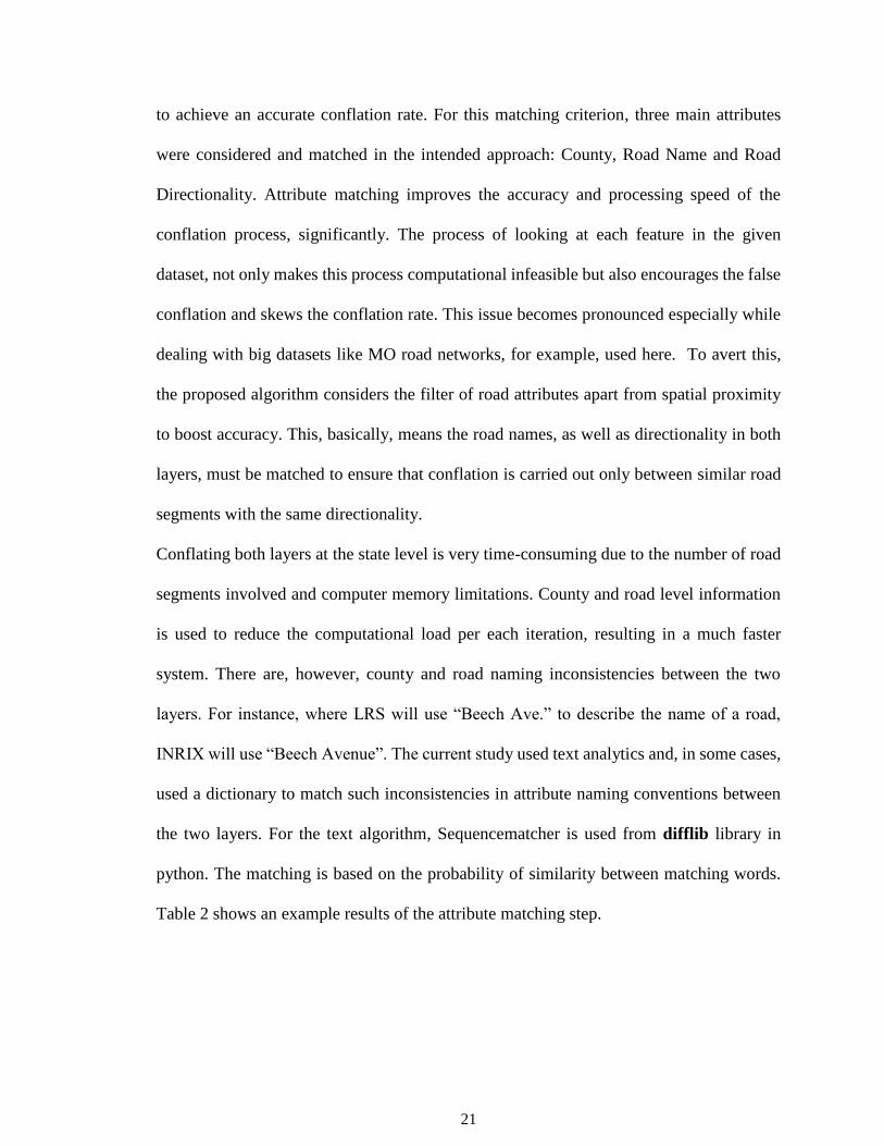
Figure 11: Conflation Rate for Interstates
From this trialing of multiple values of conflation radius, the radius of 2000 feet seemed to
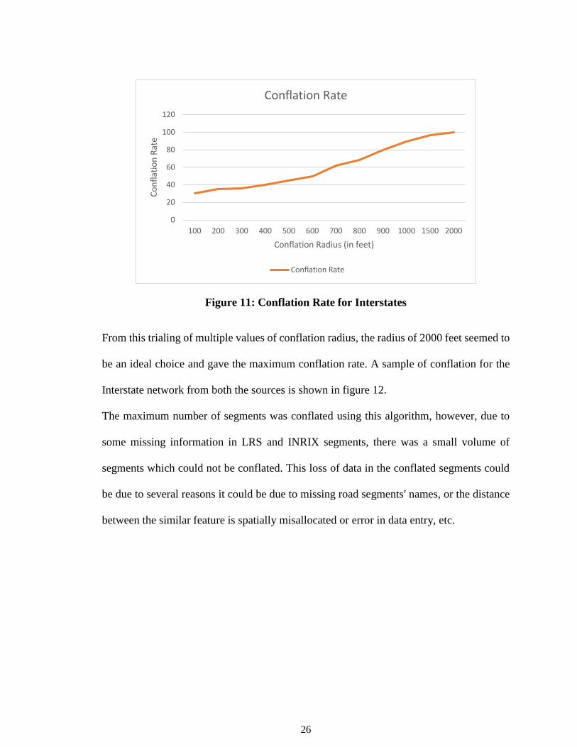
be an ideal choice and gave the maximum conflation rate. A sample of conflation for the
Interstate network from both the sources is shown in figure 12.
The maximum number of segments was conflated using this algorithm, however, due to
some missing information in LRS and INRIX segments, there was a small volume of
segments which could not be conflated. This loss of data in the conflated segments could
be due to several reasons it could be due to missing road segments' names, or the distance
between the similar feature is spatially misallocated or error in data entry, etc.
0
20
40
60
80
100
120
100 200 300 400 500 600 700 800 900 1000 1500 2000
Co
nfl
atio
n R
ate
Conflation Radius (in feet)
Conflation Rate
Conflation Rate
27
Figure 12: LRS and INRIX conflation for Interstates
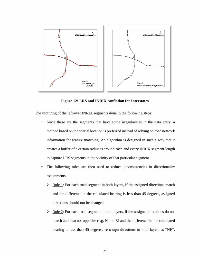
The capturing of the left-over INRIX segments done in the following steps:
o Since these are the segments that have some irregularities in the data entry, a
method based on the spatial location is preferred instead of relying on road network
information for feature matching. An algorithm is designed in such a way that it
creates a buffer of a certain radius is around each and every INRIX segment length
to capture LRS segments in the vicinity of that particular segment.
o The following rules are then used to reduce inconsistencies in directionality
assignments.
➢ Rule 1: For each road segment in both layers, if the assigned directions match
and the difference in the calculated bearing is less than 45 degrees, assigned
directions should not be changed.
➢ Rule 2: For each road segment in both layers, if the assigned directions do not
match and also not opposite (e.g. N and E) and the difference in the calculated
bearing is less than 45 degrees, re-assign directions in both layers as “NE”.
28
Similarly, for “South” and “West”, reassign as “SW”.
➢ Rule 3: For each road segment in both layers, if road directionality is not
assigned, however, the difference in the calculated bearing is less than 45
degrees, assign directions in both layers as “A-D” (Assigned Directionality).
A detailed representation of this set of procedures is shown in figure 13. In figure 13(a)
buffer size of the desired radius is drawn. Then this buffer is intersected with LRS
segments falling inside the buffer boundaries which is shown in figure 13 (b). The result
of this intersection gives LRS segments and INRIX segments with a common buffer id
which is visually represented as figure 13 (c). Now for the bearing conflation of an
INRIX segment, rather than looking for each LRS segment in the conflation radius, the
computer is going to restrict its search to buffer size and number of LRS segments
belonging to that particular buffer.
o After the intersection of two layers, now every INRIX segment will have a bunch
of LRS segments around and out of which one of them is the matching feature for
the INRIX segment. To find the matching feature the bearing of the INRIX
segment is used as a matching criterion. The bearing of each INRIX and LRS
segment is calculated based on the starting and ending longitudes and latitudes.
This bearing value is then used for matching features from both the sources. The
search radius of the buffer is selected based on the tradeoff between the conflation
rate and conflation accuracy represented in figure 14. Based on this 6m buffer
radius seemed to be optimum with a balanced tradeoff between conflation rate and
accuracy.

29
(a) (b)
(c)
Figure 13: Feature matching using bearing

30
Figure 14: Variation of Conflation Rate and Accuracy with respect to the search
radius
For this analysis, various functions from the arcpy library were employed. For the creation
of a buffer around the INRIX segment the function “buffer_analysis.” The code was run
for the buffer values from 1 meter to 20 meters and then the buffer was intersected with
LRS. Every buffer will have a unique id which would be common for both the segments
INRIX as well as LRS after the intersection.
Within the buffer, the INRIX segment was conflated to LRS based on the matching
bearing.
After accumulating a similar feature, a near table was created for every INRIX segment
using the function “GenerateNearTable_analysis” from arcpy library and the feature is
matched based on the nearest matching feature.
After finalizing the criteria for matching the features, the designed methodology uses near
table approach to match the feature from the INRIX layer to the LRS layer. Hence, the
matching feature criterion is based on two tiers for this approach:
0
10
20
30
40
50
60
70
80
90
1 2 3 4 5 6 7 8 9 1 0 1 5 2 0
PER
CEN
TAG
E
BUFFER RADIUS (IN METER)
BEARING CONFLATION
Conflation Rate Accuracy
31
a. Firstly, the segments are conflated based on the name as well as directionality from
the LRS dataset for a selected INRIX segment.
b. The segments which didn’t have directionality feature were simply conflated based
on the bearing proximity within a selected radius.
c. Then the feature is matched on the spatial proximity of INRIX segment among the
accumulated LRS segments using Near table approach
Since this approach uses multiple criteria to match features rather than just being dependent
on the spatial location of road segments the accuracy achieved through this process was
higher than the ESRI’s aforementioned process.
Transfer Attributes
The attribute is then transferred to the base layer (LRS layer in our case) as mentioned for
traditional GIS toolsets. The sample from the result is shown in table 4.
Table 4: Transfer Attribute Output Table
INRIX_ID INRIX_NAME LRS_ID LRS_NAME
119P07741 US-36 85923 36
119+16858 WORNALL RD 1644975 WORNALL ROAD
119+07741 MO-10 85923 36
119-06674 MO-34 591824 34
119-04685 I-70-ALT/I-670 976285
WYOMING ST TO
IS670W
It is evident from Figures 11 and 12 the conflation has been achieved of a decent rate and
from table 4, it was apparent that the tools were able to conflate correctly even when the
segments have a slightly different name. For example, I-70-ALT/I-670 from INRIX was
able to conflate to WYOMING ST TO IS670W in LRS irrespective of some discrepancies

32
in the name.
3.2 INRIX and Transit Conflation:
INRIX-Transit- The second pair of data sets used here are the INRIX (probe) layer and
transit data collected for Saint Louis County. This conflation of probe road networks with
the real-time location of transit data helped in getting traffic conditions on the Missouri
road networks. Traditionally, this kind of network analysis for traffic parameters like delay,
travel time, the queue length is usually done manually, as this conflation needs multi-level
analysis before dealing with actual conflation. Here the INRIX data was conflated with the
transit data collected from the Saint Louis County using the mile marker points and location
of the datasets. This transit data comprises of busses’ live locations for two weeks which
contains variables like travel time of the trip, direction, name of the route, etc. Based on
the time stamp and a unique trip id assigned to a transit system the travel time of each trip
was calculated using the distance of the route.
USE CASE: The INRIX data provides travel time for each segment. To get the delay for
a given route, firstly INRIX segments are conflated with the transit data and then the
average travel time on each route was calculated by summing all the conflated INRIX
segment’s travel time for every trip. And then the delay was calculated by getting the
difference between actual travel time take by transit and average travel time provided in
the INRIX data. The overlay of INRIX and transit data is shown in figure 15 and on the
right, the resultant conflated map of INRIX with transit data is shown. The conflation
achieved through these two data sets gives traffic-related attributes on road networks.
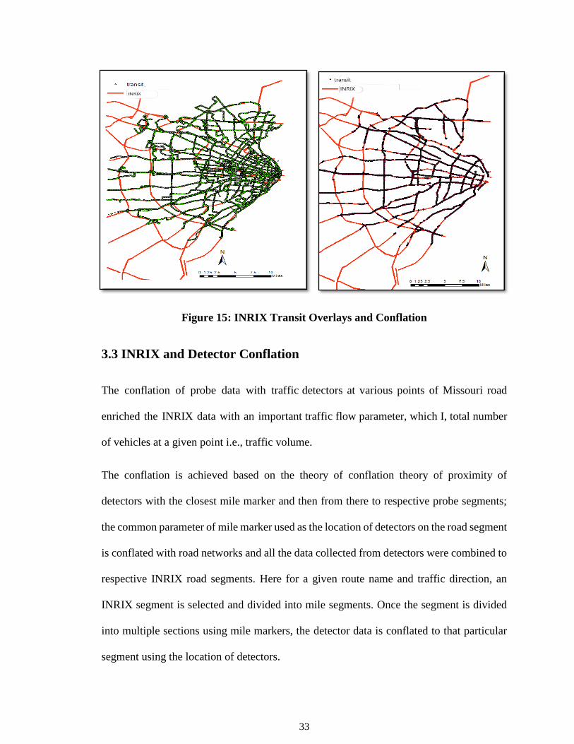
33
Figure 15: INRIX Transit Overlays and Conflation
3.3 INRIX and Detector Conflation
The conflation of probe data with traffic detectors at various points of Missouri road
enriched the INRIX data with an important traffic flow parameter, which I, total number
of vehicles at a given point i.e., traffic volume.
The conflation is achieved based on the theory of conflation theory of proximity of
detectors with the closest mile marker and then from there to respective probe segments;
the common parameter of mile marker used as the location of detectors on the road segment
is conflated with road networks and all the data collected from detectors were combined to
respective INRIX road segments. Here for a given route name and traffic direction, an
INRIX segment is selected and divided into mile segments. Once the segment is divided
into multiple sections using mile markers, the detector data is conflated to that particular
segment using the location of detectors.
34
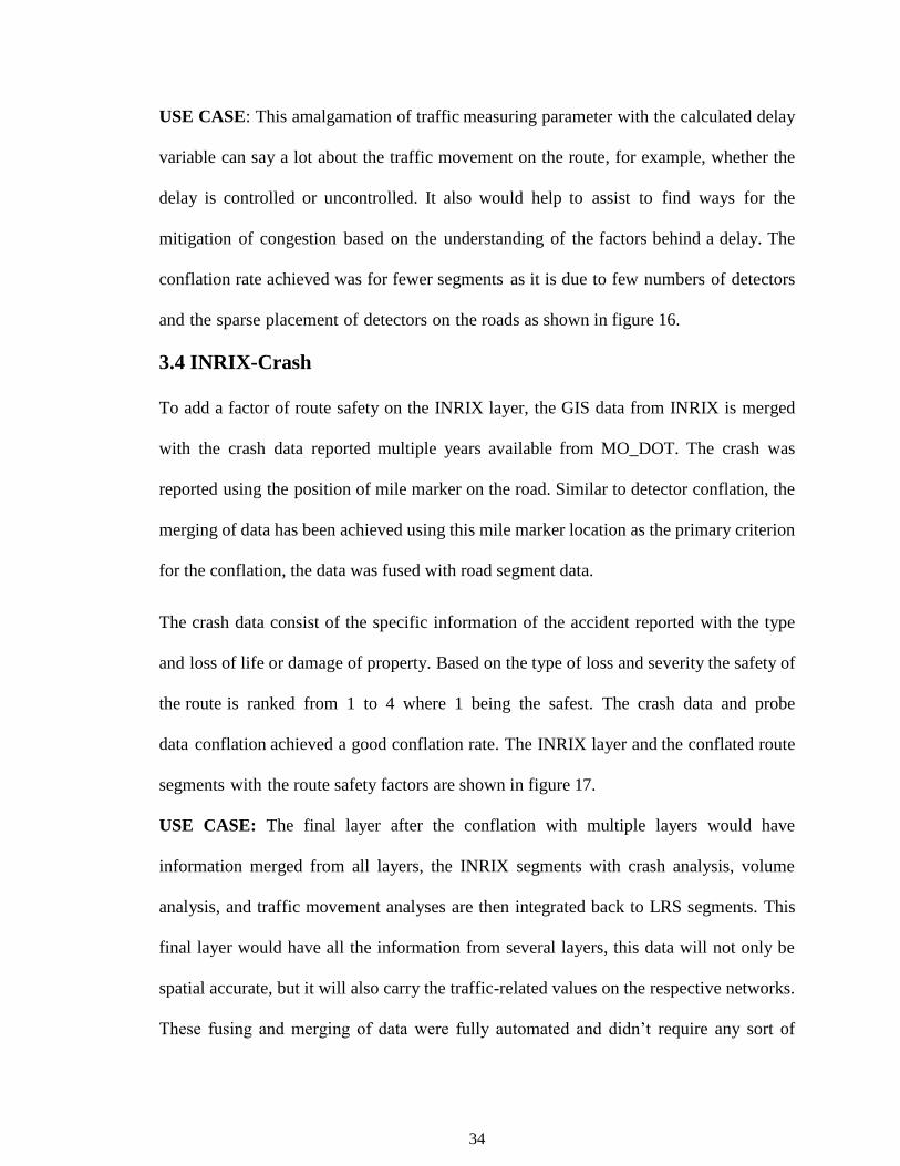
USE CASE: This amalgamation of traffic measuring parameter with the calculated delay
variable can say a lot about the traffic movement on the route, for example, whether the
delay is controlled or uncontrolled. It also would help to assist to find ways for the
mitigation of congestion based on the understanding of the factors behind a delay. The
conflation rate achieved was for fewer segments as it is due to few numbers of detectors
and the sparse placement of detectors on the roads as shown in figure 16.
3.4 INRIX-Crash
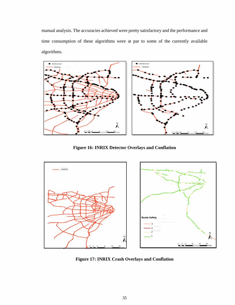
To add a factor of route safety on the INRIX layer, the GIS data from INRIX is merged
with the crash data reported multiple years available from MO_DOT. The crash was
reported using the position of mile marker on the road. Similar to detector conflation, the
merging of data has been achieved using this mile marker location as the primary criterion
for the conflation, the data was fused with road segment data.
The crash data consist of the specific information of the accident reported with the type
and loss of life or damage of property. Based on the type of loss and severity the safety of
the route is ranked from 1 to 4 where 1 being the safest. The crash data and probe
data conflation achieved a good conflation rate. The INRIX layer and the conflated route
segments with the route safety factors are shown in figure 17.
USE CASE: The final layer after the conflation with multiple layers would have
information merged from all layers, the INRIX segments with crash analysis, volume
analysis, and traffic movement analyses are then integrated back to LRS segments. This
final layer would have all the information from several layers, this data will not only be
spatial accurate, but it will also carry the traffic-related values on the respective networks.
These fusing and merging of data were fully automated and didn’t require any sort of
35
manual analysis. The accuracies achieved were pretty satisfactory and the performance and
time consumption of these algorithms were at par to some of the currently available
algorithms.
Figure 16: INRIX Detector Overlays and Conflation
Figure 17: INRIX Crash Overlays and Conflation

36
CHAPTER 4 RESULTS AND DISCUSSION
4.1 Data description:
The data involved in this research work includes-
• INRIX data,
• LRS data
• Transit data
• Detector data
• Crash data.
INRIX data- This layer of the road network has been collected from the MO_DOT RITIS
source. The data contains more detailed information about Missouri road networks, for
example, the information like name, length, and the traffic directions of the routes. A
sample of data is tabulated as table 5. This data gives travel-related data like travel time on
each segment, distance miles, location, etc. The data contains road information of
thousands of miles as 18,962 segments for the whole Missouri state.
Table 5: INRIX data set
The only drawback this data has apart from some data irregularities is the coverage of road
networks. This source of data covers a very small percentage of road networks. MO_DOT
TMC ROAD DIRECION COUNTY MILES …
119P19179
11TH ST
NORTHBOUND/11TH
ST NORTHBOUND EXIT 39B
ST. LOUIS
(CITY) 0.146498 …
119P19220 BRANCH ST EXIT 248B
ST. LOUIS
(CITY) 0.096197 ….

37
is constantly updating its road network coverage throughout the year. Currently, INRIX
XD data covers a total of 18,962 segments in the state of Missouri. The INRIX data is also
known as probe data and both the names are used interchangeably in this research work.
LRS data - On the other hand, this source contains data of road network collected from
US Census Bureau TIGER file 2016 has information like names, county, and basic
geographic details. This data has, undoubtedly, covered a higher percentage of roads of
Missouri, from local streets to interstates, nevertheless, it lacks detailed information like
the travel time, road orders, etc. A sample of data is shown in table 6 MODOT releases a
new version of the LRS every quarter. The current release has a total of 611,285 of road
segments.
Table 6: LRS data set
A comparison of both data sets viz. INRIX and LRS are shown in figure 18. This diagram
shows the difference in the magnitude of coverage of Missouri Road networks for both the
datasets.
AAT_ID COUNTY_NUM NAME DIRECTION Shape_Leng …
769944 106
DAVIDSON
LN 394.022 …
727328 106
CIMMARRON
RD 14.0569 …
1546068 108 1497 188.427 …
1583879 101 426 814.687 …
1583035 101 493 387.844 …
1583032 101 458A 383.096 …

38
Figure 18: LRS and INRIX road networks
Transit data-This layer of information possesses tracking data of the transit system in
Saint Louis county for three days in a week for two consecutive weeks viz. from June 19th
to June 26th, 2019 collected from General Transit Feed Specification (GTFS). The
collection of data has been done by calling API every 30 seconds and collected for three
days in a week for two consecutive weeks. This data brings the location of the transit system
on the road network with real-time location, timestamp, direction which helped to get an
idea about the traffic variables on the network for a given route and direction. A sample of
this data is tabulated under table 7.
Table 7: Transit data
vehicle_label trip_id route_id travel_time direction_id route_long_name …
32 ML King
- WEST 2550658 15525 56.01667 0 ML King …
32 ML King 2550658 15525 56.01667 0 ML King …

39
- WEST
32 ML King
- WEST 2550658 15525 56.01667 0 ML King 3
Detector data- The traffic data collected from the 555 detectors placed in the various
highways comes along with the vehicle count, interstates name collected from the Missouri
Department of Transportation (MODOT). The count of vehicles from every detector in the
data helps to understand the traffic flow on the respective conflated path. The mile marker,
traffic directionality and the name of the road where the detector is placed made the
conflation rate high as well as accurate. Delay calculated for every segment can be
categorized under controlled or uncontrolled based on the vehicle count for that segment
made available through this resource. The sample of this data is shown under table 8.
Table 8: Detector Dataset
detector StreetName Direction Longitude Latitude Log
MI064E000.7U I64 East -90.8286 38.80161 0.7
MI064E002.0U I64 East -90.8113 38.79101 1.98
MI064E003.2U I64 East -90.7914 38.7794 3.2
MI064E004.6U I64 East -90.7717 38.76682 4.6
MI064E005.6U I64 East -90.7582 38.75364 5.6
MI064E007.1U I64 East -90.743 38.73782 7.13
MI064E008.5U I64 East -90.7262 38.72309 8.49
MI064E009.1D I64 East -90.7043 38.7141 9.1
MI064E009.8D I64 East -90.6916 38.7118 9.8
40
MI064E010.0D I64 East -90.69 38.7118 10
Crash data – this last traffic history database collected for Missouri’s roads helps to
visualize the road segments from the safety point of view. The crash data congregated based
on the mile marker has the details of accidents like type, severity, conditions during the
accident as well as the environment around like road surface, visibility, weather, etc. The
severity of an accident can be pointed out based on the number of factors like vehicles
involved, whether it was loss of property or life, etc. This data has been collected from state
DOT for the analysis.
This conflation of these datasets with Probe and subsequently with LRS developed the
conflated layer with analyzed traffic data variables like travel time, route reliability, traffic
volume, etc. At the time of writing this report, the most current versions of both data layers
(IRIX and LRS) were used. In the following section, we evaluate the effectiveness of the
conflation approach developed for this study.
4.2 Conflation Result Discussion
Probe with LRS – this conflation aimed to enrich the LRS layer with the information of
roads found in probe (INRIX) layer like travel time, the direction of traffic, and other routes
related information. Nonetheless, due to the diversity of the datasets, this conflation
required special attention. Rather than conflating just based on the spatial parameter, this
algorithm addressed the issue of data anomaly and inaccuracies by taking consideration of
route configurations. By matching the attributes of the county, road name, and traffic
directionality of the matching feature and then conflating based on the location proximity
of matching features from the near table boosted the accuracy as well as the conflation rate.
Since the attribute chosen for roads was unique the mis conflation was zero, this code was

41
tested for all the interstates for Missouri state and gave the results as shown in figure 19.
The perfect accuracy attainted for interstates was mainly due to high similarity in the
nomenclature adopted for the interstates designations, for example, LRS uses the number
of interstates as road names while Probe data uses the number of interstates with “I”. So,
in LRS Interstate 29 is presented as “29” on the other hand in probe data it is labeled as “I-
29.” The algorithm of text similarity was able to capture this minute difference and hence
the accuracy, as well as the conflation rate provided, was so high. The conflation rate was
98.9 % with 100% accuracy.
Figure 19 Conflation Rate and Accuracy for Interstates.
On the other hand, when this conflation was tried for whole MO road networks, the overall
conflation rate achieved was 86%. The lack of conflation rate was mainly due to missing
attribute features such as traffic directionality or names as well as limitations of text
similarity algorithm which was unable to detect subtleties in the way nomenclature was
adopted.
For such conflation, a more sophisticated tool was employed instead of just being
30 35 36 40 45 50 62 68 80 89 97 98.9
100 100 100 100 100 100 100 100 100 100 100 100
1 0 0 2 0 0 3 0 0 4 0 0 5 0 0 6 0 0 7 0 0 8 0 0 9 0 0 1 0 0 0 1 5 0 0 2 0 0 0
PER
CEN
TAG
E
CONFLATION RADIUS (IN FEET)
Conf lat ion for interstates
Conflation Rate Accuracy
42
dependent on spatial proximity. After the creation of buffer around every Probe segment
and intersecting with surrounding LRS segments, the algorithm uses the concept of bearing
to conflate the similar segment. Since this tool was more advance than spatial conflation,
it was able to achieve higher accuracy as shown in figure 20. The accuracy achieved was
72% with the trade of conflation rate of 73%.
Figure 20: Conflation rate and accuracy for bearing
Due to the high dependency on physical aspects of data, the conflation rate achieved was
decent and the accuracy was adequate. The conflation rate, as well as accuracy of few
selected segments, were tabulated under table 9. The dip in these parameters was mainly
due to lack of data and mis conflation, since there were no governing attribute parameters,
the mis conflation was pretty high.
The higher accuracy achieved for certain segments was mainly due to proximity as well as
similar laying of the shapefiles, however, certain segments were mis conflated or not
conflated have many factors attached for such outcomes. The details for this table are
discussed in the conflation discussion.
0
10
20
30
40
50
60
70
80
90
1 2 3 4 5 6 7 8 9 10 15 20
Per
cen
tage
Buffer Radius (in meter)
Conflation using Bearing
Conflation Rate Accuracy

43
Table 9 Conflation rate and Accuracies for few Major roads
Road Name Conflation Rate Accuracy
Airport Road 0.947 0.647
ADELAIDE AVE 1 1
CLARK AVE 0.03 0
LACLEDES LANDING
BLVD
0.01 0
FOREST PARK PKWY 0.2 0.09
IS44W TO IS270E 0.24 0.04
IS44E TO LAFAYETTE
AVE
0.1 0.06
BROADWAY TO IS64W 0.32 0.04
N AIRPORT BLVD 1 0.69
STADIUM BLVD 1 0.79
WYANDOTTE ST 1 0.85
S JEFFERSON AVE 1 0.91
WILSON AVE 1 0.714
WESTRIDGE RD 1 1
US-54-BR/MARKET ST 0.48 0
N ELSON ST 0.9 0.14
W 39TH ST 1 0.8
WALNUT ST 0.98 0.93
W KANSAS ST 0.6 0.5
Probe with Transit - this conflation was done to gather traffic variables for the different
routes. The live location of transit was conflated with the Probe layer to enrich the road
network with traffic data like travel time, average speed, route credibility, etc. All the
INRIX segments are gathered for a unique trip id based on the conflation. The average time
given for individual probe segments is gathered and averaged for that particular trip. The
distance was calculated based on the miles per trip gotten from the summation of conflated
probe segments. The timestamp given for a trip gives an actual idea about the actual travel
time taken for that trip, on the other hand, probe data gives on an average time that should
have taken by the vehicle on that segment. The difference in the travel time of these two
datasets gives the traffic flow parameters like delay, travel time credibility, etc. An

44
interactive dashboard that can be generated using the fusion of this data is shown in figure
21. The overall accuracy achieved was 85% for these datasets. Since the study was only
considering Saint Louis County, the interaction of all the probe segments with transit data
couldn’t be captured.
Probe with detector - The probe data is conflated with the detector file separately and
the layer
has been enriched subsequently with the information gathered from the detectors at the
various locations in Missouri. The detector data contributed vehicle count related to the
traffic flow on respective positions which subsequently conflated with t h e INRIX layer
making the respective road network supplemented with traffic data like traffic volume
with the direction of the traffic. The basic common variable for this conflation was the
position of detectors found out by the mile marker. This conflation eventually merged with
LRS_INRIX conflated to transfer the data to the resultant layer. The accuracy of conflation
has been modest with a value of 80%. The less accuracy of these datasets mainly due to the
sparse placement of detectors (mainly on Interstates). The traffic volume achieved can be
fused with travel time could give a brief idea about travel time credibility as well as
congestion type. Such an analysis is shown in figure 22.
45
Figure 21: Travel time interactivity
Figure 22: TITAN Interactive Dashboard for exploring statewide mobility

46
Probe-Crash - The crash INRIX conflated data helped to add a factor of route safety on
the map.
Based on the route safety factor the route choice and demand of the segments could be used
while dealing with the travel model. The safety number assigned to a route dependent on
factors like the number of crashes, type of crashes (KABCO- fatality, property damage,
etc.) This route safety could have also been used to get an overall safety analysis of
Missouri road networks.
Eventually, this conflated probe data with traffic as well as crash data are conflated with
LRS to achieve the final layer of road segments with augmented information of the routes
as well as the expected travel experience parameters like travel time, delay as well as the
route safety based on the previous accidents. The accuracy of the respective conflation is
tabulated in table 10.
Figure 23:Statewide safety mobility dashboard

47
Table 10: Conflation Rates for the various layers
With this reasonable accuracy for multiple merging of layers to get a final map with
improved spatial data as well as relevant traffic variables, the desired layer of LRS with
the aforementioned data is achieved. The data shared in table 11 gives an idea about the
information the final layer is going to possess after conflation through all the conflated
layer data.
A superimposed image of all these layers and the visualization of one of the parameters
for these datasets viz. delay is shown as in figure 24.
After conflating all the data segments, a visual dashboard was created with the help of the
tool OmniSCI. In figure 24, the parameter for travel time has been visualized. The color
variation from green to red shows the increase in the travel time for Saint Louis County
obtained from the transit data set. This software gives on-click visualization and analysis
for all the parameters involved and could help immensely for the visualization of big data
S.N
o
Conflati
on
Acc
ura
cy
1 INRIX_Transit 85%
2 INRIX_Detector 80%
3 INRIX_Crash 80%
4 LRS_INRIX 95%
5 GIS LRS_INRIX 48%
48
like this in the field of transportation engineering. The travel time parameter visualization
in the figure categorizes road segments using delay parameter for the Saint Louis county;
with the red being of highest delay and green with no delay. This kind of imagining of the
conflated layer gives a quick idea about the current status of road segments with respect to
parameters of interest.
Figure 24: Overlay of all conflated layers and travel time visualization
Table 11: Final conflated layer
LRS_I
D
C
O
ROA
D
DI
R
INR_ID
MIL
ES
Travel
time
Dela
y
Volum
e
Rout
e
Safet
y
86647 11 US-36 E 119+0773
9
0.60
6
0.76 0.55 365 1
796991 13 US-36 E 119+0728 8.989 8.25 6.73 365 1

49
3
87197 11 US-54 E 119+0986
3
2.14 2.17 4 370 2
86658 11 US-54 E 119P0774
0
0.506 0.55 0.48 370 2
86953 11 US-60 E 119+0986
4
4.36 6.69 5 300 1
797013 13 IS-70 E 119+0986
0
10.76 9.78 7.21 370 2
87475 13 LP-70 E 119+0728
1
9.76 9.13 4.56 148 2
86239 11 MO-
150
W 119P07741 0.497 0.61 0.2 295 3
86970 11 OR-
150
E 119+0986
3
2.1 2.17 1.66 120 4
87269 11 US-36 E 119+0727
6
4.1 3.91 1.43 365 1

50
4.3 Challenges with the current results
One of the important challenges incurred during automating the conflation process,
especially for such a big scale is a false correlation or false conflation. The workflow
for map conflation developed in the current study also generates incorrect results in
certain situations and these challenges could be mainly due to:
• Text similarity
• Bearing Error
• Segment lengths
• GIS errors
• Data error
Text Similarity- Another thing that has been unfolded through this study which was
hindering the conflation process significantly was the difference in the data labeling.
One of the most basic challenges faced during the merging of information from different
sources is the variance between the ways the nomenclature has been implemented.
Although the data has the same geographic features and locations, it still fails to get
conflated or mis-conflated due to the absence of standard formatting of labels. The
most common one is the difference in the name of the same features; different sources have
their unique ways to store the information. Basic things like “-”, “,”, “.”, spellings,
abbreviations become a great obstacle to overcome during conflation, especially, when the
data is big and complicated. The rectification of this issue demands robust computational
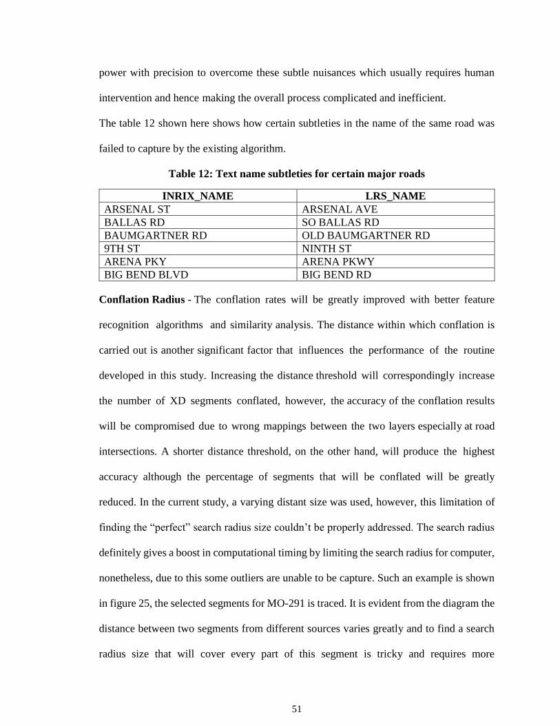
51
power with precision to overcome these subtle nuisances which usually requires human
intervention and hence making the overall process complicated and inefficient.
The table 12 shown here shows how certain subtleties in the name of the same road was
failed to capture by the existing algorithm.
Table 12: Text name subtleties for certain major roads
INRIX_NAME LRS_NAME
ARSENAL ST ARSENAL AVE
BALLAS RD SO BALLAS RD
BAUMGARTNER RD OLD BAUMGARTNER RD
9TH ST NINTH ST
ARENA PKY ARENA PKWY
BIG BEND BLVD BIG BEND RD
Conflation Radius - The conflation rates will be greatly improved with better feature
recognition algorithms and similarity analysis. The distance within which conflation is
carried out is another significant factor that influences the performance of the routine
developed in this study. Increasing the distance threshold will correspondingly increase
the number of XD segments conflated, however, the accuracy of the conflation results
will be compromised due to wrong mappings between the two layers especially at road
intersections. A shorter distance threshold, on the other hand, will produce the highest
accuracy although the percentage of segments that will be conflated will be greatly
reduced. In the current study, a varying distant size was used, however, this limitation of
finding the “perfect” search radius size couldn’t be properly addressed. The search radius
definitely gives a boost in computational timing by limiting the search radius for computer,
nonetheless, due to this some outliers are unable to be capture. Such an example is shown
in figure 25, the selected segments for MO-291 is traced. It is evident from the diagram the
distance between two segments from different sources varies greatly and to find a search
radius size that will cover every part of this segment is tricky and requires more
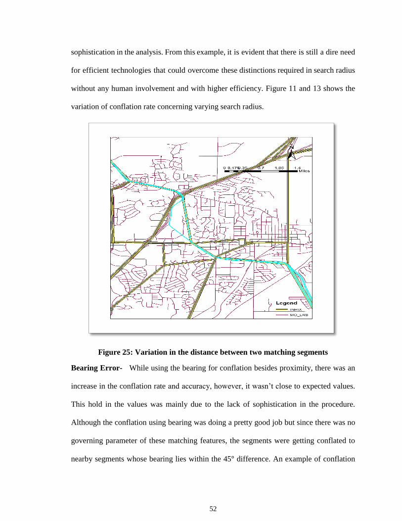
52
sophistication in the analysis. From this example, it is evident that there is still a dire need
for efficient technologies that could overcome these distinctions required in search radius
without any human involvement and with higher efficiency. Figure 11 and 13 shows the
variation of conflation rate concerning varying search radius.
Figure 25: Variation in the distance between two matching segments
Bearing Error- While using the bearing for conflation besides proximity, there was an
increase in the conflation rate and accuracy, however, it wasn’t close to expected values.
This hold in the values was mainly due to the lack of sophistication in the procedure.
Although the conflation using bearing was doing a pretty good job but since there was no
governing parameter of these matching features, the segments were getting conflated to
nearby segments whose bearing lies within the 45° difference. An example of conflation
53
using bearing for Kansas Street is given in figure 26; on the left side, Kansas street is
selected for INRIX data and on the right side the selected segments which had been
conflated for that street. If looked closely, the segments on the right were mis conflated to
Kansas Street, even though the right segment was right there.
This limitation of bearing can be overcome if it has been coupled with some governing
parameters like unique data information or some computational capability to assign
segments based on more matching physical aspects like size, shape, direction, etc.
Figure 26:Bearing Conflation for Kansas St
Segment lengths- The conflation is primarily based on spatial joining of features from
different map layers, and due to the presence of diverse form and shapes of road
segments, this process becomes unusually challenging to achieve if targeting for an
unbiased conflation between two features on large-scale data. The influence of segment
length is much more when there is no other attribute feature addressing mis conflation. If a curve
and straight segments are present close enough to a feature from another layer, the

54
conflation could be challenged by the theory of proximity; the features would be matched
based on the closeness rather than other authentic parameters like direction and name. Also,
when the segment length is more and curvy it tends to mis conflate especially as the
alignment of segments are constantly changing. When segments are very small, it loses the
capability of individuality and gets conflated to any nearest segment. The influence of
segment length in the conflation rate is shown in figure 27. This biasedness could be
overcome by using more sophisticated computational algorithms that can differentiate
between the subtleties in the segment length as well as shape.
Figure 27: Influence of segment length in conflation rate
GIS errors- The improper position of geographies in the map layers is also another
important contest encountered by researchers when it comes to merging the spatially
different maps. These features are much more complicated and ambiguous especially when
data have been gathered from numerous sources. These discrepancies become prevalent
in geometric structures like highway interchanges, roundabouts with multiple ramps and
winding roads probably due to the complexity of road networks and inefficient
0.10.06
0.58
0.82
0.68
0.36
0.510.44
0.33
0.460.41
0 - 0.1 0.1-0.2 0.2-0.3 0.3-0.4 0.4-0.5 0.5-0.6 0.6-0.7 0.7-0.8 0.8-0.9 0.9-1.0 1.0+
Co
nfl
atio
n R
ate
(%)
Segment Length
Influence of Segment Length

55
computational tools. These incongruities in the location of features could lead to false
conflation and overall absurd information. This error was evident when testing the size of
the conflation radius.
Data Issue: While dealing with data there were many issues with the reporting of
information. This algorithm has tried to overcome such irregularities by filtering the data
as much as possible. However, the issues like missing data and error in reporting the names
of data were difficult to target. As there was no significant pattern in such errors it was
hard to prepare a set of procedures targeting such issues. For example, Interstate 29 (I-
29)in the INRIX layer was reported as US-21, then some routes had some segments
missing, altogether. Figure 28 shows one such problem, in the LRS data is shown in
highlighted blue color whereas the same I-44 is reported with some error in INRIX
shapefile (on the right). Such types of issue were difficult to address and were one of the
major reasons for hampering the rate as well as the accuracy of this conflation algorithm.
This type of issue could be addressed through a sophisticated computational tool or some
sort of artificial intelligence that can detect such manual errors.

56
Figure 28: I-44 from LRS and INRIX layer
4.4 Concluding Remarks and Recommendations
This project develops a methodology for the automatic conflation of two geographic data
layers: TIGER’s LRS and MODOT’s Probe segments and extended to traffic data and crash
data available for the state of Missouri. This work is sprouted to improve the overall
effectiveness of the conflation process. Rather than confining the focus on improving
specific geo-related information regarding routes, it was a good idea to take this merging
process to different types of database to achieve a layer of map which has much more
pertinent parameters which would help DOTs to keep an overview of all the road
segments with respect to relevant parameters in return it would help in increasing the
overall travel experience on these roads. So far, the calculation of specific traffic-related
parameters was done manually and due to its complexities and the large dataset size, they
were confined to specific areas of interest. Being said that, there were many aspects of
conflation that have been unfurled during different phases of this project which needs

57
attention to make this procedure much more productive. The protruding one would be a
conflation of GIS data with traffic and crash data; although it has done a satisfactory job
when it comes to bringing the traffic parameters in the spatial data and improving the overall
quality of road segments, still lacks the complete effectiveness of these conflations due to
meager precision. A slightly lower accuracy of these INRIX conflations achieved with
different layers could be mainly due to the following two reasons:
• Computational methods- The technology available and the algorithm employed
could be not efficient enough to overcome the nuances encountered during this
process. For example, the GIS errors in reporting the crash data or sparsely uneven
distribution of detectors, etc., could lead to poor accuracy. Nonetheless, these
anomalies could be easily overcome by using an advanced and specific algorithm
that takes on these different tones of data available out there.
• Data- The other prominent thing which had been tricky to handle was the diverse
nature of all these data. Probably one algorithm is incapable of handling these
varied forms of reports and database employed for achieving this conflation. This
could be easily and significantly improved by advancing the data collection
methods by the inculcation of technologies to improve the overall quality of data
and minimize the false reporting of information as much as possible. At a conflation
rate of 95%, there is still a lot of room for improvement. The following
recommendations will be critical to achieving a more appreciable conflation rate.
• Considerable improvement in conflation rates can be achieved if robust pattern
matching algorithms are used instead of relying solely on in-built ArcGIS feature
matching models. There have been improvements in the development of spatial

58
pattern matching algorithms recently in the open GIS community. Tapping into this
resource will be useful.
• A thorough comparative analysis of all Esri’s ArcGIS tools for map conflation
should be conducted. In the current project, only the rubber sheet tool was explored.
Other conflation tools were not explored and compared to the existing algorithm.
• For complicated features such as interchanges and roundabouts, this study suggests
a manual procedure for the conflation process.
• A more consistent and unified framework for defining road segment directionality
should be communicated to all vendors. Due to the inconsistent assignment of
directions to road segments, the current study used the start and end
latitude/longitudes (bearing) to recompute the directionality of each segment in
both geographic layers. When conflating longer segments to shorter ones,
computed directionality can be misleading. With the available tools and
technology, this work was able to achieve satisfactory results and opened doors
to achieve conflation for various types of databases which could help to eradicate
the manual calculation of these parameters. Also, this work would encourage us to
have these parameters analysis handy rather than make it available as per
requirements. Nonetheless, a lot can be done to take this study to different levels and
fields of transportation, especially, when it comes to handling big transportation data
for the analysis of different variables.
• The handling of missing data could be handled more efficiently for example the
uses of tools like mean substitution, regression imputation, last observation

59
carrying forward, etc., could help to do accurate analysis even if there is an issue of
data irregularities.
• Hashtable could be an appropriate way to achieve higher text similarity accuracy.
By defining some common combinations in the hashtable the text-similarity
algorithm can be improved significantly. Combinations like ‘PKWY’, ‘PKY’;
‘Avenue’, ‘ST’ etc., are some combinations that can be zipped using a hashtable.
The choice of combinations could be better analyzed by doing some explanatory
analysis of these combinations.
• Accuracy- The conflation accuracy achieved could be better justified based on the
field where it has been implemented. The travel time, delay, route time credibility
are some parameters that could be used in the field of traffic and can be used for
the planning of future roadways as well. Higher accuracy is a requirement for the
planning area as it defines policy for future development. The traffic flow
parameters delay as well as traffic count could be employed to get an idea about
traffic problems like the type of congestion, controlled or uncontrolled. Since the
analysis has to be made from the current study, these areas require a more
sophisticated tool to achieve a higher rate of conflation. On the other hand,
conflation related to crashes gives some transportation safety-related parameters
like route safety based on the type of crashes as well as the severity of crashes. The
requirement of accuracy for this conflation is not tight and a decent rate is
acceptable, however, further studies need to be coupled with the current conflation
as the crash frequency is a sensitive parameter and supplementary research is a
requirement.

60
REFERENCES
1. Arulselvi, S., Karthik, B. and Sundararajan, M., A frame work for road network extraction
from remotely sensed high resolution images. International Journal of Pure and Applied
Mathematics, 116.
2. C.-C. Chen, S. Thakkar, C.A. Knoblok, and C. Shahabi. BAutomatically annotating and
integrating spatial datasets, in Proceedings of the International Symposium on Spatial and
Temporal Databases, Santorini Island, Greece, 2003.
3. Chen, C.C., Knoblock, C.A. and Shahabi, C., 2006. Automatically conflating road vector
data with orthoimagery. GeoInformatica, 10(4), pp.495-530.
4. Lynch, M.P. and Saalfeld, A.J., 1985, March. Conflation: Automated map compilation—
a video game approach. Proceedings Auto-Carto (Vol. 7, pp. 343-352).
5. Rosen, B.; Saalfeld, A., 1985, March Match criteria for automatic alignment.
Proceedings Autocarto (Vol. 7, 11–14, pp. 1–20).
6. Lupien, A.E. and Moreland, W.H., 1987. A general approach to map conflation.
Proceedings of 8th International Symposium on Computer Assisted Cartography
(AutoCarto 8).
7. Saalfeld, A., 1988. Conflation automated map compilation. International Journal of
Geographical Information System, 2(3), pp.217-228.
8. Cobb, M.A., Chung, M.J., Foley III, H., Petry, F.E., Shaw, K.B. and Miller, H.V., 1998. A
rule-based approach for the conflation of attributed vector data. GeoInformatica, 2(1),
pp.7-35.
61
9. Yuan, S. and Tao, C., 1999. Development of conflation components. Proceedings of
Geoinformatics, 99, pp.1-13.
10. Beller, A., Doytsher, Y. and Shimbersky, E., 1997. Practical Linear Conflation in an
innovative software environment. Proceeding of 1997 ACSM/ASPRS.
11. Thakkar, S. and Knoblock, C.A., 2003, August. Efficient Execution of Recursive
Integration Plans. In IIWeb (pp. 169-174).
12. Michalowski, M., Ambite, J.L., Thakkar, S., Tuchinda, R., Knoblock, C.A. and Minton,
S., 2004. Retrieving and semantically integrating heterogeneous data from the web.
IEEEIntelligent Systems, 19(3), pp.72-79.
13. Olteanu, A., Mustière, S. and Ruas, A., 2006, July. Matching imperfect spatial data. In
Caetano, M., Painho, M.(Es.), Proceedings of 7th International Symposium on Spatial
Accuracy Assessment in Natural Resources and Environmental Sciences. Lisbon (pp. 7-9).
14. Butenuth, M., Gösseln, G.V., Tiedge, M., Heipke, C., Lipeck, U. and Sester, M., 2007.
Integration of heterogeneous geospatial data in a federated database. ISPRS Journal of
Photogrammetry and Remote Sensing, 62(5), pp.328-346.
15. Kyriakidis, P.C., Shortridge, A.M. and Goodchild, M.F., 1999. Geostatistics for conflation
and accuracy assessment of digital elevation models. International Journal
of Geographical Information Science, 13(7), pp.677-707.
16. Cobb, M.A., Petry, F.E. and Shaw, K.B., 2000. Fuzzy spatial relationship refinements
based on minimum bounding rectangle variations. Fuzzy sets and systems, 113(1), pp.111-
120.

62
17. Edwards, D. and Simpson, J., 2002. Integration and access of multi-source vector data.
INTERNATIONAL ARCHIVES OF PHOTOGRAMMETRY REMOTE SENSING AND
SPATIAL INFORMATION SCIENCES, 34(4), pp.167-174.
18. Ruiz, J.J., Ariza, F.J., Urena, M.A. and Blázquez, E.B., 2011. Digital map conflation: a
review of the process and a proposal for classification. International Journal of
Geographical Information Science, 25(9), pp.1439-1466.
19. Brovelli, M.A. and Zamboni, G., 2004. Adaptive transformation of cartographic bases by
means of multiresolution spline interpolation. Int Arch Photogram Rem Sens Spatial
Inform Sci, 35, pp.206-211.
20. . Hacar, M. and Gökgöz, T., 2019. A New, Score-Based Multi-Stage Matching Approach
for Road Network Conflation in Different Road Patterns. ISPRS International Journal of
Geo-Information, 8(2), p.81.
21. Mustière, S. and Devogele, T., 2008. Matching networks with different levels of detail.
GeoInformatica, 12(4), pp.435-453.
22. Huh, Y., Yu, K. and Heo, J., 2011. Detecting conjugate-point pairs for map alignment
between two polygon datasets. Computers, Environment and Urban Systems, 35(3),
pp.250-262.
23. Ruiz, J.J., Ariza, F.J., Urena, M.A. and Blázquez, E.B., 2011. Digital map conflation: a
review of the process and a proposal for classification. International Journal of
Geographical Information Science, 25(9), pp.1439-1466.
24. Samal, A., Seth, S. and Cueto 1, K., 2004. A feature-based approach to conflation of
63
geospatial sources. International Journal of Geographical Information Science, 18(5),
pp.459-489.
25. Xiong, D. and Sperling, J., 2004. Semiautomated matching for network database
integration. ISPRS journal of photogrammetry and remote sensing, 59(1-2), pp.35-46.
26. Volz, S., 2006. An iterative approach for matching multiple representations of street
data. International Archives of Photogrammetry, Remote Sensing and Spatial Information
Sciences, 36(Part 2/W40), pp.101-110.
27. Zhang, M., 2009. Methods and implementations of road-network matching (Doctoral
dissertation, Technische Universität München).
28. Doytsher, Y., Filin, S. and Ezra, E., 2001. Transformation of datasets in a linear-based map
conflation framework. Surveying and Land Information Systems, 61(3), pp.159-169.
29. Volz, S., 2006. An iterative approach for matching multiple representations of street
data. International Archives of Photogrammetry, Remote Sensing and Spatial Information
Sciences, 36(Part 2/W40), pp.101-110.
30. Haunert, J.H., 2005, July. Link based conflation of geographic datasets. In 8th ICA
workshop on generalization and multiple representation, A Coruña, Spain.
31. Li, L. and Goodchild, M.F., 2011. An optimisation model for linear feature matching in
geographical data conflation. International Journal of Image and Data Fusion, 2(4),
pp.309-328.
32. Xiong, D. and Sperling, J., 2004. Semiautomated matching for network database
integration. ISPRS journal of photogrammetry and remote sensing, 59(1-2), pp.35-46.

64
33. Yang, B., Luan, X. and Zhang, Y., 2014. A Pattern‐ Based Approach for Matching Nodes
in Heterogeneous Urban Road Networks. Transactions in GIS, 18(5), pp.718-739.
34. Fan, H., Yang, B., Zipf, A. and Rousell, A., 2016. A polygon-based approach for matching
OpenStreetMap road networks with regional transit authority data. International Journal
of Geographical Information Science, 30(4), pp.748-76.
35. Image Courtesy - GIS Geography https://gisgeography.com/conflation-edgematching-
rubbersheeting/