AUTOMATED DESIGN OF APPLICATION-SPECIFIC

SUPERSCALAR PROCESSORS

by

Tejas Karkhanis

A dissertation submitted in partial fulfillment of

the requirements for the degree of

Doctor of Philosophy

(Electrical Engineering)

at the

UNIVERSITY OF WISCONSIN – MADISON

2006

© Copyright by Tejas Karkhanis 2006

All Rights Reserved

i

Abstract

Automated design of superscalar processors can provide future system-on-chip (SOC)

designers with a key-turn method of generating superscalar processors that are Pareto-optimal

in terms of performance, energy consumption, and area for the target application program(s).

Unfortunately, current optimization methods are based on time-consuming cycle-accurate

simulation, unsuitable for analysis of hundreds of thousands of design options that is required

to arrive at Pareto-optimal designs. This dissertation bridges the gap between a large design

space of superscalar processors and the inability of cycle-accurate simulation to analyze a

large design space, by providing a computationally and conceptually simple analytical

method for generating Pareto-optimal superscalar processor designs.

The proposed and evaluated analytical method consists of three parts: (1) a method for

analytically estimating the performance in terms a cycles-per-instruction (CPI) using the

application program statistics and the superscalar processor parameters, (2) a method of

analytically estimating various energy consuming activities using the application program

statistics and the superscalar processor parameters, and (3) a method of finding the Pareto-

optimal designs using the CPI and energy activity models. At the hearts of these three parts

are analytical equations that model the fundamental governing principles of superscalar

processors. These equations are simple yet accurate enough to quickly find the Pareto-optimal

superscalar processor designs.

ii

In addition to the computational simplicity, the analytical design optimization method

is conceptually simple. It gives clear conceptual design guidance by providing (1) the ability to

visualize the performance degrading events, such as branch mispredictions and instruction

cache misses, (2) the ability to analyze energy consuming activity at the microarchitecture

level, and (3) a cause-and-effect relationship between superscalar core design parameters. The

conceptual simplicity allows a quick grasp of the analytical method and also provides key

insights into the inner workings of superscalar processors.

The overall analytical design optimization method is orders of magnitude faster than

cycle-accurate simulation based exhaustive search and Simulated Annealing methods. On a

2GHz Pentium-4 machine, the analytical method requires 16 minutes to arrive at Pareto-

optimal designs from a superscalar design space of about 2000 feasible designs. On the same

machine and for the same design space, it is estimated that exhaustive search and Simulated

Annealing methods require 60 days and 24 days, respectively. In addition, the analytical

method arrives at the same Pareto-optimal designs as the exhaustive search method. In

contrast, Simulated Annealing is unable to find all Pareto-optimal designs.

Analytical method’s firm foundation in the first principles of superscalar processors enables

the analysis of superscalar processor design spaces with hundreds of thousands of design

options and application programs with large number of dynamic instructions. As a result the

proposed analytical design optimization method can provide future SOC designers with a

key-turn approach to generate Pareto-optimal application-specific superscalar processors with

minimal design time and effort.

iii

Dedication

This dissertation is dedicated to my family.

iv

Acknowledgements

I thank my advisor, Jim Smith, for making this research possible. He has endured me

through my undergrad research, Master’s research, and PhD research. Throughout he has

taught me a lot about research, engineering, and writing. His keen insight and words of

wisdom have transformed me into a better person and a better engineer. Jim is a model that I

will try to emulate throughout my career.

Professors Mark Hill, Volkan Kursun, Mikko Lipasti, and Mike Schulte did much more

than just serve on my thesis proposal and defense committees. They have always had a

welcoming smile and encouraging words for me. They provided me with important advice and

insights on academic as well as non-academic issues.

I thank Daniel Leibholz and Pradip Bose for being excellent mentors during my

internships in the industry. In summer of 2000, Daniel Leibholz gave me the opportunity to

experience a microprocessor architect’s role in a microprocessor product team at SUN

Microsystems. This experience ignited my interest in various aspects of computer design. In

summers of 2001, 2002, and 2003 Pradip Bose guided me through industrial research at IBM

Thomas J Watson Research Center and IBM Research Triangle Park. Ultimately it was Pradip’s

encouragement and guidance that put me on the path of the PhD.

Gordie Bell, Ho-Seop Kim, Trey Cain, and Bruce Orchard kept the condor cluster and

ECE computers up and running. This condor cluster enabled me to perform the 2000+

simulation required to evaluate my thesis research.

v

Saisanthosh Balakrishnan and Kevin Moore have been my close friends during the grad

school. The coffees, lunches, and dinners provided us with many opportunities for discussing

research and life. My sincere thank to Sai and Kevin for providing crucial feedback on my

thesis proposal and this dissertation.

I was honored to share 3652 with Woo-Seok Chang, Kyle Nesbit, Nidhi Agarwal,

Shiliang Hu, Ashutosh Dhodapkar, Ho-Seop Kim, Sebastien Nussbaum, and Tim Heil.

Sebastien helped me settle in graduate level research during my first year of grad school.

During my final year, Woo-Seok and Nidhi provided key feedback on my thesis proposal and

this dissertation.

Above all, I am blessed to have a wonderful family. They always had unwavering faith

in my abilities, even when I did not. My mother, Prajakta, and father, Sunil, inculcated in me

the value of education that enabled me to pursue PhD research. They never accepted the

answer “Its going OK” when asked about my research. My brother, Rohan, has always been an

unlimited source of encouragement, inspiration, and laughter. He never let me forget the lighter

and more important aspects of life when I was stressed out to meet a conference deadline. My

wife, Monal, always provided a positive view on my research even when there seemed

insurmountable hurdles. I thank you for your patience and the stability that you have

provided in my life. The real future work beings now, with us writing the chapter of our life

together.

Finally, I acknowledge the funding sources that made this research possible. This work

was supported by SRC contract 2000-HJ-782, NSF grants CCR-9900610, CCR-0311361, and

EIA-0071924, IBM, and Intel. Any opinions, findings, and conclusions or views expressed in

this dissertation are mine and do not necessarily reflect the views of the funding sources.

vi

Contents

Abstract ........................................................................................................................................i

Dedication...................................................................................................................................iii

Acknowledgements.....................................................................................................................iv

Contents......................................................................................................................................vi

Chapter 1: Introduction..............................................................................................................1 1.1 Motivation........................................................................................................................1 1.2 Contribution: Analytical Design Optimization Approach..................................................6 1.3 Dissertation Organization ...............................................................................................8

Chapter 2: Design Optimization Methods................................................................................10 2.1 Heuristic Methods ..........................................................................................................10 2.2 Reduced Input-Set Method...............................................................................................12 2.3 Trace Sampling Methods.................................................................................................13 2.4 Statistical Simulation......................................................................................................15 2.5 First-order Methods .......................................................................................................17 2.6 Summary ........................................................................................................................21

Chapter 3: CPI Model...............................................................................................................22 3.1 Basis ..............................................................................................................................22 3.2 Top-level CPI Model ......................................................................................................27 3.3 Program Statistics..........................................................................................................29 3.4 The iW Characteristic ....................................................................................................31

3.4.1 Unbounded Issue Width ...........................................................................................32 3.4.2 Bounded Issue Width ..............................................................................................34 3.4.3 Modeling Taken Branches........................................................................................37

3.5 Branch Misprediction Penalty ........................................................................................40 3.6 Instruction Cache Misses ...............................................................................................48 3.7 Data Cache Misses.........................................................................................................51 3.8 CPI Model Evaluation....................................................................................................58

3.8.1 Evaluation Metrics ...................................................................................................59

vii

3.8.2 Correlation between analytical model and simulation...............................................60 3.9 Summary ........................................................................................................................65

Chapter 4: Energy Activity Model ...........................................................................................67 4.1 Quantifying Energy Activity ...........................................................................................68

4.1.1 Combinational logic................................................................................................68 4.1.2 Memory cells ..........................................................................................................69 4.1.3 Flip-flops ................................................................................................................69 4.1.4 Modeling Miss-speculated Activities........................................................................71 4.1.5 Insight provided by the ASI method ........................................................................72 4.1.6 ASI method versus Utilization method.....................................................................72

4.2 ASI Method Validation ...................................................................................................74 4.3 Top-level Analytical Modeling Approach .......................................................................75 4.4 Components based on combinational logic.....................................................................80

4.4.1 Function Units ........................................................................................................80 4.4.2 Decode Logic..........................................................................................................82

4.5 Components based on memory cells ...............................................................................84 4.5.1 L1 instruction cache ................................................................................................84 4.5.2 Branch Predictor .....................................................................................................85 4.5.3 Level 1 Data Cache .................................................................................................87 4.5.4 Level 2 Unified Cache.............................................................................................89 4.5.5 Main Memory .........................................................................................................91 4.5.6 Physical Register File..............................................................................................92

4.6 Components based on flip-flops......................................................................................94 4.6.1 Reorder Buffer ........................................................................................................94 4.6.2 Issue Buffer.............................................................................................................96 4.6.3 Pipeline stage flip-flops...........................................................................................98

4.7 Analytical Model Evaluation ........................................................................................ 100 4.7.1 Evaluation Metrics ................................................................................................ 101 4.7.2 Correlation between analytical model and simulation............................................ 102 4.7.3 Histogram of differences: Are the differences random? ......................................... 106

4.8 Summary ...................................................................................................................... 107

Chapter 5: Search Method...................................................................................................... 109 5.1 Overview of the Search Method.................................................................................... 109 5.2 Superscalar Pipeline Optimization ............................................................................... 111 5.3 Evaluation of the proposed Design Optimization method.............................................. 119

5.3.1 Evaluation Metrics ................................................................................................ 120 5.3.2 Workloads and Design Space ................................................................................. 120 5.3.3 Coverage of analytical method and e-constrained method ..................................... 121 5.3.4 False positive rates of compared methods.............................................................. 122 5.3.5 Correlation of Pareto-optimal curves...................................................................... 124 5.3.6 Time complexity of baseline, proposed, and conventional methods ........................ 125 5.3.7 Analysis of results.................................................................................................. 129

5.4 Comparison Analytical Method with Industrial Processor Implementations ................. 130 5.5 Summary ...................................................................................................................... 133

viii

Chapter 6: Conclusions........................................................................................................... 135 6.1 Future Work................................................................................................................. 140

References................................................................................................................................ 142

1

Chapter 1: Introduction

Analytically-based design optimization methods can complement cycle-accurate

simulation in designing application-specific superscalar processors, yielding orders of

magnitude optimization speedup over current methods. This dissertation presents a

computationally and conceptually simple design optimization method for out-of-order

superscalar processors. The computational simplicity enables analysis of a large number of

design alternatives in a relatively short time period. Its conceptual simplicity enables a quick

grasp of the method and also provides key insights into the workings of superscalar processors

that can guide cycle-accurate simulations. In essence, the new design optimization method

bridges a long-standing gap between the large number of superscalar design options provided

by integrated circuit technology and the limitations of cycle-accurate simulations in quickly

evaluating a large number of designs.

1.1 Motivation

Processors are used in virtually every electronic device sold today. In some products

such as handheld computers and games, the presence of a processor is evident, but in most of

them, for example, smart phones, digital cameras, and DVD players, the processor(s) are

embedded. In every such product, the marketplace is constantly demanding increased

functionality and performance. The diversity of products, the number of companies producing

them, energy consumption, cost, and the importance of time-to-market places a premium on

2

producing processors that are optimal for the particular product being designed – application-

specific processors.

Market requirements and advances in integration have led to system-on-chip (SOC)

designs. A typical SOC has a general-purpose microprocessor core (including level-1

instruction and data caches), a level-2 cache, auxiliary processors and accelerators, and

peripheral components connected to each other by on-chip buses. The general-purpose micro-

processor carries out a variety of functions, and the accelerators focus on specific tasks, e.g.,

graphics or DSP. The peripherals are controllers for off-chip systems such as the main

memory, a graphics display system, network interface, and USB port(s). The SOC designer

chooses from the available general-purpose processor cores, accelerators, and peripherals to

design a system that fits in the allocated chip area and meets the energy consumption and

performance targets. Due to market demands the SOC designer must complete the design

within the time-to-market that is required for the product.

Product requirements constantly demand increased functionality and higher

performance. This has caused the evolution of embedded processor microarchitectures to

evolve along the same path as high performance general-purpose processors, although lagging

by a few years. Embedded processor evolution began with multi-cycle sequential processors

and then went to simple in-order pipelines, followed by more complex in-order designs,

including features such as branch prediction. Today, in-order embedded superscalar cores like

IBM PowerPC 405[1] and out-of-order embedded superscalar cores such as MIPS R10000[2,

3], PowerPC 440[4], NEC’s VR55000[5] and VR77100[6] Star Sapphire, and SandCraft’s

SR710X0 64-bit MIPS microprocessor[7] are available. The eventual widespread use of

superscalar processors in performance-intensive embedded products is inevitable.

3

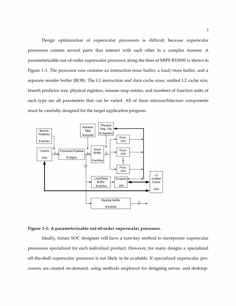
Design optimization of superscalar processors is difficult because superscalar

processors contain several parts that interact with each other in a complex manner. A

parameterizable out-of-order superscalar processor along the lines of MIPS R10000 is shown in

Figure 1-1. The processor core contains an instruction issue buffer, a load/store buffer, and a

separate reorder buffer (ROB). The L1 instruction and data cache sizes, unified L2 cache size,

branch predictor size, physical registers, rename map entries, and numbers of function units of

each type are all parameters that can be varied. All of these microarchitecture components

must be carefully designed for the target application program.

Figure 1-1: A parameterizable out-of-order superscalar processor.

Ideally, future SOC designers will have a turn-key method to incorporate superscalar

processors specialized for each individual product. However, for many designs a specialized

off-the-shelf superscalar processor is not likely to be available. If specialized superscalar pro-

cessors are created on-demand, using methods employed for designing server- and desktop-

4

class microprocessors, either future SOC designers will have to be superscalar processor design

experts, or a superscalar processor expert will be required for every application specific

superscalar processor. Furthermore, every processor to be designed will also require a logic

design team, a circuit design team, and a simulation farm with perhaps hundreds or

thousands of computers. Due to the complexity of the design process, it currently takes five to

seven years to develop a new superscalar microprocessor [8]. This time-to-market is

unacceptable for application specific products, where the typical time-to-market is around

eight to twelve months [9].

An alternative is to first provide a superscalar core composed of scalable,

parameterized components, for example, issue ports, issue and reorder buffers, caches, branch

predictors, and functional units. Next, an SOC designer provides the application program(s),

upper bounds on acceptable area and energy, and a lower bound on acceptable performance.

Then, based on the characteristics of the application(s) and the available parameterized

components, an automated design framework produces a set of superscalar processor designs

that provide the best tradeoffs for performance, energy, and area. This set of designs is termed

as “Pareto-optimal” in the field of Multi-Objective Optimization [31][32]. From this set of

Pareto-optimal designs, the SOC designer can select one of the designs that meet the

performance, energy, and area targets (if such a design exists). In this way design automation

will enable the design of application-specific superscalar processors with minimal design time

and effort.

The automated design framework studied in this dissertation has three principal parts:

a parameterizable superscalar processor, a component database, and a design optimization

method. The parameterizable superscalar processor was illustrated in Figure 1-1. It specifies the

pre-designed components and interconnections between the components that form the

5

processor core. The component database stores pre-designed components, such as issue buffers,

function units, reorder buffers, register files, and caches, along with their silicon area and

energy consumption. The design optimization method examines the application program, the

component database, and the parameterizable superscalar processor and arrives at the Pareto-

optimal superscalar processor designs.

The design optimization method is at the heart of the automated design framework. It

has a performance model, energy model, area model, and a search method that work together

to arrive at the Pareto-optimal designs. The performance and energy models use a

configuration’s microarchitecture parameters and characteristics of the application software to

compute performance and energy consumption, respectively. The area model computes the

total area of the superscalar processor configuration by first finding the area occupied by each

pre-designed component and then summing the individual component areas. The search

method navigates the superscalar processor design space, using the performance, energy, and

area models, to find the Pareto-optimal configurations.

A naïve optimization approach is to use cycle accurate simulations for generating CPI

and energy activity estimates of the program for all possible design options. Area for all design

options can be computed with the simple addition of individual areas of the pre-designed

components from the component database. Then, the search method can select the designs that

are Pareto-optimal in terms of CPI, energy, and area. This naïve method will certainly find all

Pareto-optimal designs. Unfortunately, the naïve method is impractical for generating the

Pareto-optimal designs in a timely manner, because cycle accurate simulations are time-

consuming.

As an alternative to the naïve method, current design optimization methods either

analyze only a few designs from the hundreds of thousands of designs that are provided, or

6

they analyze only a few dynamic instructions of the application programs from the millions of

instructions that may constitute a program. The small number of designs to analyze are

chosen by complementing cycle-accurate simulation with ad hoc, heuristic-based optimization

methods such as Simulated Annealing[10-13]. Similarly, methods that select a small number

of dynamic instructions from the original program do so with ad hoc means. Consequently, the

small number of dynamic instructions may not represent the original program.

1.2 Contribution: Analytical Design Optimization Approach

The design optimization method developed in this dissertation is based on analytical

equations that model the fundamental governing principles of superscalar processors. With

this method a small number of designs are selected from a large superscalar design space in a

systematic manner, using mathematical and statistical reasoning. The proposed method uses

fundamental program statistics, such as data dependences, functional unit mix, cache miss-rate,

branch misprediction rates, and load statistics, collected with computationally simple, one-time

trace-driven analysis of the program. Because the proposed method is driven by the first

principles of superscalar processors, ad hoc optimization methods are not required. Overall, the

new method provides a clear and simple approach for optimizing superscalar processors.

The new optimization method is comprised of a first-order performance model that

estimates cycles per instruction (CPI), a first-order energy activity model that is used to

compute energy consumption, area model, and a first-order search method that finds Pareto-

optimal designs. The CPI and energy activity models provide a computationally simple way

to estimate CPI and energy activity, respectively. The area model simply adds the areas of the

individual components of the superscalar processors design. The search method uses the

model insights to systematically find Pareto-optimal designs for the target application

7

program. Afterwards, only the Pareto-optimal designs are evaluated with cycle-accurate

simulations to produce more precise CPI and energy activity estimates. This technique

significantly reduces optimization time while retaining the accuracy of the naïve, cycle-

accurate simulation based exhaustive search.

This dissertation provides more than just an optimization method. The CPI model,

energy activity model, and the search method are each important in their own regard.

The first-order CPI model provides a method of visualizing performance degrading

events. That is, the issue rate can be graphed as a function of clock cycles when a performance

degrading event occurs. This not only provides a basis for a mathematical development of the

performance loss, but also provides a way to clearly analyze the impact of the performance

degrading event. The CPI model can provide quick design feedback and insights into how to

decrease performance losses due to various performance degrading events.

The energy activity model provides a method of quantifying energy at the

microarchitecture level. This allows the processor designer to view the microarchitecture in a

technology independent manner when considering energy of the final design. The first-order

methods developed for computing energy activities are based on the same fundamental

principles as the CPI model. Consequently, the energy activity model can provide a

spreadsheet-like method for estimating energy consumption at early stages of superscalar

processor design.

The search method provides a divide-and-conquer method for balancing the

superscalar pipeline, branch predictor, and caches. Because of the divide-and-conquer

approach, the superscalar processor subsystems can be analyzed and optimized in isolation.

This ability is important for engineering conceptually complex systems, in general.

8

1.3 Dissertation Organization

The next chapter gives background on design optimization methods. First, design

optimization of superscalar processors is put in a historical perspective. This is followed by a

survey of previous design optimization methods. Along the way aspects that distinguish the

proposed method from the previous methods are discussed.

Chapter 3 develops the first-order CPI model. This model employs an “independence

approximation”. That is, the added CPIs due to various performance degrading miss-events,

such as cache misses and branch mispredictions, are computed independently, in isolation of

each other. Individual CPI computation uses the program statistics and relies on the

fundamental principles of superscalar processors. Overall, the proposed CPI model is accurate

with respect to detailed simulation and provides a computationally simple method for

estimating the CPI.

Chapter 4 develops the energy-activity model. The model quantifies energy at the

microarchitecture level in terms of three types of energy activities. First, the energy activities are

defined. Then, first-order methods for computing the energy activities are developed. Energy

activity computation uses the program statistics and leverages the basic underlying methods

developed for the execution time model. The independence approximation is employed to

quickly calculate the energy activities. Model evaluation is also presented in this chapter.

Evaluation indicates that the analytical energy activity model tracks cycle-accurate simulation

and provides a computationally simple method for estimating energy activities and ultimately

the energy consumption.

Chapter 5 describes the new search method that exploits insights derived from the first-

order CPI and energy activity models and employs a clear and simple divide-and-conquer

approach. The chapter shows how the search method drives the CPI and energy activity

9

models. The divide-and-conquer approach is also described in detail. The chapter concludes

with a comparison of the analytically-based overall design optimization method with cycle-

accurate simulation based exhaustive search and with Simulated Annealing. The results show

that the new design optimization method is always orders of magnitude faster than the

exhaustive search method and the Simulated Annealing method.

Finally, chapter 6 provides a summary of the design optimization problem. Limitations

of current design optimization methods and the contributions of this thesis are also

summarized. The chapter concludes the dissertation with a discussion of potential future

research.

10

Chapter 2: Design Optimization Methods

Currently available design optimization methods roughly fall into the following five

categories: 1) heuristic methods, 2) reduced input-set methods, 3) sampling methods, 4)

statistical simulation, and 5) first-order methods. Design optimization methods in the first

category reduce the number of superscalar designs that must be analyzed. Those in the

second, third, and fourth categories aim to increase the simulation efficiency, thereby

decreasing the overall time to find the Pareto-optimal designs. The methods in the last

category aim at eliminating cycle-accurate simulation. The proposed optimization method is

closely related to the first-order methods.

2.1 Heuristic Methods

In early 1980’s, Kumar and Davidson employed a quasi-Newton heuristic and

developed a cycle-accurate simulation based optimization technique [14]. To reduce the

design optimization time, their method also uses a six parameter linear equation. The

parameters of the linear equation are found by first performing several cycle accurate

simulations at various design points in the design space and then curve fitting the linear

equation to the observed performance values.

After calibrating the linear equation, the design space is explored with the equation and

the quasi-Newton method[15] until an optimal design is found; this is called the predicted

optimum. Cycle-accurate simulation is performed at the predicted optimum design point. If

11

the performance value generated with the model is within some range of the value generated

by the simulation, sensitivity analysis is performed. Otherwise, if there is a disparity between

the model and simulation performance values, the entire process restarts from the calibration

step.

During sensitivity analysis, the design points within some neighborhood of the

predicted optimal design are evaluated with cycle-accurate simulations to determine if the

optimal design was predicted correctly. The search for an optimal design continues until the

following two conditions are met: 1) the analytical model and the cycle-accurate simulation

arrive at the same performance estimate for the predicted optimal, and 2) the sensitivity

analysis indicates that the predicted optimal design is indeed optimal.

Kin et al. [16] complemented cycle-accurate simulation with Simulated Annealing.

Their simulated annealing algorithm first tentatively selects a design. Next, a new design is

selected at random from the pool of designs that have not been analyzed. If the initial design is

better than the new design, the new design is discarded. But, if the new design is better than

the initial design, the initial design is discarded and replaced by the new design. This process

of selecting a new design and comparing it to a currently optimal design continues until the

objective being optimized converges to a value or the algorithm reaches the upper limit on the

number of designs that can be analyzed. The design that is considered optimal at the time

algorithm stops is selected.

A key disadvantage of current heuristic methods is that the unit being optimized is

“black-boxed”. That is, heuristic methods provide design parameters to the simulation model

and observe the output of the simulation. Heuristics algorithms are not based on insight as to

how to optimize the superscalar processor; consequently heuristic algorithms can get stuck in

12

local minima [14, 15] and can arrive at a non-optimal design without explicitly indicating that

the design is non-optimal.

2.2 Reduced Input-Set Method

An alternative approach for reducing design optimization time is to reduce the

simulation time. One way to reduce cycle-accurate simulation time is to analyze a small

number of dynamic instructions from program trace. There are two methods for achieving this

goal: 1) modify the program inputs such that the new trace will be much shorter than the

original trace, and 2) select a small number of instructions from the original program trace that

will faithfully represent the original program. Methods in the first category are referred to as

reduced input-set methods, and are discussed in this section. Methods in the second category

are referred to as trace-sampling methods and are discussed in the subsequent section.

The first approach of modifying program inputs was proposed by Osowski and

Lilja[17]. The authors apply sampling at the inputs of SPECcpu2000 programs to generate a

sampled version called MinneSPEC. They either simply truncate the program inputs, or

modify the inputs to generate the sampled trace. The authors justify MinneSPEC by

comparing its instruction mix profile to the instruction mix profile of SPECcpu2000.

Unfortunately, experimental evidence suggests that reduced input-set methods are not

ideal for designing out-of-order superscalar processors. Eeckhout and De Bosschere employ

statistically rigorous methods and show that performance estimates produced with reduced

input-set methods do not track those of the original program [18]. The authors employ

Principal Component Analysis and Clustering Analysis and show that simply because the

MinneSPEC tracks the instruction-mix profile of the SPECcpu2000 does not imply that their

13

performance estimates will also track each other. Another comparative study [19], arrived at

the same conclusions as Eeckhout and De Bosschere.

2.3 Trace Sampling Methods

A better alternative to reduced input-set methods is to first generate an instruction

trace by functionally simulating the program with the full input, and then sample the resulting

instruction trace; this process is called trace sampling. In one of the first applications of trace

sampling to processor simulation, Conte [20] randomly selected a small number of instruction

sequences from the program trace. From the trace analysis of program about 20,000

consecutive dynamic instructions are traced, and then some 50 million instructions are

skipped. This tracing and skipping process continues until the entire benchmark is executed.

The sampled trace drives the cycle accurate simulator, instead of the program trace.

Sherwood et al. used basic block profiles to select small number of instructions from

the program [21, 22]. During trace analysis of the program a count of the number of times

every basic block is entered is measured for every interval of length 100 million dynamic

instructions. After the entire trace is analyzed, basic block profiles of all intervals are compared

to identify repetitive parts in the program.

Instruction intervals with similar basic block profile are grouped together and the

sample trace is constructed by selecting one interval from each group. The Manhattan distance

of the basic block profiles of a pair of intervals provides a numerical value that represents the

similarity between the two intervals. Finally, the Manhattan distance values are analyzed by a

clustering algorithm and groups of intervals with similar basic block profiles are created. One

instruction interval from each group is then selected to form the sampled trace.

14

A key limitation of the trace sampling methods is the inability to represent cache miss

rates for L2 caches. The Conte and Sherwood et al. methods correlate trace samples with the

instruction mix profile of the program, not the cache miss rates. For programs with large

working sets, misrepresenting cache miss rates in the sample trace can introduce errors in

execution time and energy estimation.

Wunderlich et al. presented a sampling method based on feedback from cycle-accurate

simulation [23]. First, there is an initial guess of the number of instructions to analyze with

cycle accurate simulation in one sample and also the number of samples. During this initial

simulation, variation in cycles per instruction (CPI) is measured for every sample for the entire

program trace. If the CPI variation is such that the estimate is not in the desired confidence

interval, the number of instructions within a sample and the number of samples necessary to

bring CPI variation within a desired confidence interval is predicted. The benchmark is

analyzed again with the new parameters for the number of samples and the number of

instructions per sample. This process continues until the variation of CPI of the samples is

within the desired confidence interval.

The authors claim that at the benchmark has to be analyzed at most two times to have

the CPI variation within the desired confidence interval. When this method is not performing

cycle-accurate simulations, it performs functional simulation and updates state based

structures, for example caches and branch predictor, in the cycle accurate simulator.

The feedback directed sampling method has an advantage over the Conte and

Sherwood methods because it directly attempts to minimize CPI error. However, the drawback

of the feedback directed method is that the prediction of the number of instructions that must

be analyzed with cycle accurate simulation is based on CPI error estimation from the previous

interval. The prediction does not guarantee that CPI error will be within the desired confidence

15

bound. Consequently, there is no guarantee that the overall CPI error with Wunderlich method

will be within the desired confidence bound.

Fields et al. developed a sampling and analysis technique based on genome sequencing

[24]. For one instruction out of every 1000 instructions, a detailed account of microarchitecture

events that take place during its execution is recorded from the underlying cycle accurate

simulation. The recorded information is transformed into a graph that represents the

microarchitecture events. This process is performed for every sampled instruction.

Next, individual instruction execution graphs are concatenated to construct what the

authors call a microexecution graph. The concatenation is enabled by a two-bit signature,

recorded for instructions before the sampled instruction and for instructions after the sampled

instruction. This microexecution graph is analyzed for identifying performance bottlenecks and

for design optimization [25, 26].

The insights from the Fields et al. method are gained after a reference cycle-accurate

simulation. With their method there are no guarantees that the same sampling method will

represent instruction execution phenomenon in another (optimized) microarchitecture

configuration. Another drawback is that their current implementation does not model the

queuing delay in the issue buffer and bounded issue width on instruction execution.

2.4 Statistical Simulation

Statistical simulation is an alternative to sampling methods for reducing the number of

instructions that must be analyzed. Statistical simulation generates a sequence of synthetic

instructions based on program characteristics. Cache and branch predictor miss-rates are

measured with functional simulations of the program trace. Based on these statistics cache

16

and branch predictor misses are generated; the miss rates are approximately equal to miss

rates of the program.

Nussbaum and Smith [27] perform a trace-driven simulation of application program

and collect program statistics such as instruction dependence probabilities, instruction mix,

branch misprediction rate, L1 data cache miss rate, L2 data miss rate, L1 instruction cache

miss rate, and L2 instruction miss rate. Based on these statistics they generate synthetic

instruction traces and assume miss-events that have similar statistical characteristics as the

program. The synthetic instructions are taken from a simplified instruction set that contains a

minimal set of 14 instructions types. These synthetic instructions and miss-events drive a

simplified cycle accurate simulator. The process of synthetic instruction generation followed by

simulation continues until the performance converges to a value; this process typically requires

tens to hundreds of thousands of synthetic instructions.

Eeckhout [28] collects the same basic statistics as Nussbaum and Smith. However, for

constructing instruction dependences he collects more detailed statistics on registers and

memory such as degree of use of register instances, age of register instances, useful lifetime of

register instances, lifetime of register instances, and age of memory instances. Then, he curve

fits the register dependence statistics to a power-law equation. Next, synthetic instructions are

generated based on the dependence characteristics modeled by the power-law equation. The

synthetic miss-events are generated with a table lookup in a data structure that stores the

miss-event statistics. The combination of synthetic instructions and miss-events drives a cycle

accurate simulator. The process of synthetic trace generation followed by simulation continues

until the instruction throughput converges to a value.

Oskin et al. [29] collect statistics on the basic block size, instruction dependence

distribution, cache miss rates, and branch misprediction rates. The authors use program

17

statistics to construct a synthetic binary. The synthetic binary contains taken and not-taken

paths that follow basic block sequences and have the same characteristics of the original

program binary. This synthetic binary drives a cycle-accurate simulator. The cycle-accurate

simulations are run multiple times and the performance values are recorded. The final

performance is the average of the recorded performance values.

Recently, Eyerman et al. developed an optimization method based on statistical

simulation and heuristic methods [30]. Eyerman et al. employ heuristic methods to arrive at

small number of designs; they evaluate these designs with statistical simulation. They

compared various heuristic algorithms and found that genetic algorithm performed the best

for statistical simulation among the chosen candidate algorithms.

The advantage of statistical simulation over sampling methods is the ability to more

precisely represent the cache and branch predictor miss-rates for programs with large working

sets. Unfortunately, statistical simulations black-box the superscalar pipeline and therefore do

not provide insights into the inner workings of superscalar processors. Consequently, a

separate statistical simulation for each superscalar pipeline/cache/predictor configuration is

required.

2.5 First-order Methods

Simulation, in general, does not provide guidance for reducing execution time, reducing

energy, or for finding an optimal design. Alternatively, first-order methods provide conceptual

guidance and view of the processor with which execution time, energy, and optimization

related questions are easy to answer.

In one of the earliest instruction level parallelism studies, Riseman and Foster observed

that given a sequence of S consecutive instructions from a program, the longest dependence

18

chain is about square-root of S instructions [31]. More recently, Michaud et al. made the same

observation and developed an analytical model for instruction fetch and issue [32, 33]. To

support the square-root model, Michaud et al. perform a trace-driven simulation of a set of

software applications.

Because the average ILP will be determined by the length of longest dependence chain,

Michaud et al. compute the average ILP for a processor with issue buffer size S as the total

number of instructions executed divided by the length of the longest dependence chain for

sequences of length S. Therefore, average issue rate is modeled as the square-root of the

number of instructions examined. However, the authors do not model bounded issue width

and cache and branch predictor misses.

Hartstein and Puzak presented a first-order model for analyzing the effect of front-end

pipeline on the execution time [34]. The authors later extended their model to study the effects

of front-end pipeline length on power dissipation[35]. Two important parameters of their

model, the degree of superscalar processing and the fraction of stall cycles per pipeline stage,

are generated with cycle accurate simulations.

Noonburg and Shen [36] proposed an analytical model for the design space exploration

of out-of-order superscalar processors. Their model breaks down the instruction level

parallelism (ILP) into machine parallelism and program parallelism. Each type of parallelism is

modeled and analyzed in isolation, and then their effects are combined to arrive at the average

ILP of the application software. Program parallelism in their model is the inherent parallelism

of the application software and is composed of two parts: 1) a control parallelism distribution

function, and 2) a data parallelism distribution function. Both of the program parallelism

functions are measured with trace-driven simulation of the application software. Machine

parallelism is the amount of parallelism a specific microarchitecture can extract. The machine

19

parallelism is divided into three parts: 1) branch parallelism distribution, 2) fetch parallelism

distribution function, and 3) issue parallelism distribution function. These distributions are

modeled as vectors and matrices and are multiplied together to arrive at the average ILP value

for the application software.

There are several limitations to the Noonburg and Shen model. Their distribution

matrices assume every operation takes a single cycle to complete, so they do not model the

performance effects of non-unit function unit latencies. The reorder buffer is not modeled; only

the issue buffer is modeled. More importantly, their method does not model clock cycle

penalties associated with branch mispredictions, instruction cache misses, and data cache

misses. Because the columns of the distribution matrices must sum to one, the matrix can only

model the mean resource requirements of the application program. Consequently, their method

does not enable design of a superscalar processor for varying resources requirements of the

program. Several researchers have observed that in reality application software goes through

phases [37]. A mean-value approach by itself is insufficient because sizing various processor

resources for the average behavior can result in a non-optimal design [38, 39].

Taha and Wills [40] propose an approach that measures the number of instructions

between branch mispredictions -- called “macro-blocks” -- and then estimates performance for

each macro-block. They estimate the performance using the model proposed by Michaud et al.

[32]. To determine performance under ideal conditions Taha and Wills employ two sets of

cycle accurate simulations. The first set of simulations generates the issue rate for a spectrum

of issue buffer sizes. The second set of cycle accurate simulations generates the retire rate for a

spectrum of reorder buffer sizes.

In modeling the reorder buffer, Taha and Wills assume that all instructions that have

completed execution can retire if enough commit bandwidth is available. Consequently, their

20

method does not model the clock cycles spent in the reorder buffer by instructions that have

completed out-of-order and are waiting for preceding instructions in program order to

commit. This method will erroneously design a smaller reorder buffer than required.

Taha and Wills method assumes that the non-unit latency function units will not affect

the issue rate of instructions out of the issue buffer. Doing this essentially does not model the

bypass network and more importantly it breaks instruction dependences. It has been observed

that non-unit latency function units significantly affect the issue rate and the sufficient number

of issue buffer entries[32, 41]. As a result, the number of issue buffer entries that their method

arrives at may be insufficient for achieving the instruction throughput that is required.

Another disadvantage of Taha and Wills method is that effect of L1 data cache misses

and the loads that miss in the L2 cache are not modeled. They mention that extra clock cycles

due to data cache misses can be simply added together and their result added to the ideal

performance. However, research has shown, through careful reasoning and analysis [41, 42],

that data cache misses are not as straightforward to model as Taha and Wills suggest. L1

data cache misses are often hidden because of the issue buffer [41], and the loads that miss in

the L2 unified cache must be analyzed for overlaps [41, 42].

In general, current available first-order methods model limited aspects of out-of-order

processors. Further, they employ mean-value analysis (MVA)[43]. While MVA is important for

estimating CPI and energy, MVA does not account for the variation in resources requirements

of the program. Consequently, the resulting microarchitecture will be designed for average

requirements of the program.

This thesis generalizes an analytical first-order design optimization method based on

the governing principles of out-of-order superscalar processors. It uses fundamental statistics

of the application program collected with computationally simple, one-time trace driven

21

simulations. It provides a way to design superscalar processor resources by modeling the

variation in program‘s resource requirements. With the new method, the need to calibrate

mathematical equations with cycle accurate simulations is eliminated. More importantly, the

new method provides clear and simple conceptual guidance for designing out-of-order

superscalar processors.

A CPI model of the new design optimization method is developed in the next chapter.

The methods described in that chapter also form the foundation of the energy model and the

search process, developed in chapters 4 and 5, respectively.

2.6 Summary

In summary, cycle accurate simulations are impractical for analyzing a large number of

superscalar designs. Current, commonly used method optimize either by analyzing a small

number of designs, or by analyzing a small part of the application program. Previously

proposed first-order methods are insufficient for design optimization for two reasons: 1) they

model limited aspects of out-of-order superscalar processors, and 2) they do not model the

variation in the program’s resource requirements.

22

Chapter 3: CPI Model

Estimating performance of target program(s) running on a specific microarchitecture

configuration is one of the three essential parts of a microarchitecture optimization method. In

this research, I build a performance model around the commonly used Cycles per Instruction

(CPI) metric. In order to optimize application-specific superscalar processors, the CPI model

is applied to a large number of designs, each executing application program(s) with large

number of dynamic instructions. This requires the CPI performance model to be very efficient

so that the processor is designed within its time-to-market constraint.

This chapter develops a first-order analytical CPI performance model for out-of-order

superscalar processors. The CPI model is based on the governing principles of superscalar

microarchitecture and the program statistics mentioned in Chapter 1. This chapter contains an

evaluation of the CPI model by comparing its performance estimates to CPI values generated

with detailed, cycle-accurate simulation. The results show that the model is both

computationally simple and provides insights into the operation of superscalar processors.

The method for searching the design space developed in Chapter 5 employs the CPI model for

fast automated microarchitecture optimization.

3.1 Basis

The basis for the CPI model development to follow is illustrated in Figure 3-1. The

figure shows a graph of performance, measured in useful instructions issued per cycle (IPC),

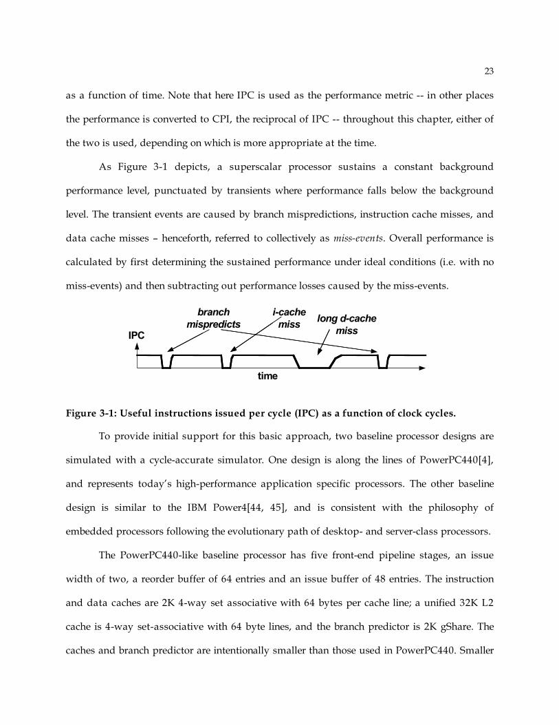
23

as a function of time. Note that here IPC is used as the performance metric -- in other places

the performance is converted to CPI, the reciprocal of IPC -- throughout this chapter, either of

the two is used, depending on which is more appropriate at the time.

As Figure 3-1 depicts, a superscalar processor sustains a constant background

performance level, punctuated by transients where performance falls below the background

level. The transient events are caused by branch mispredictions, instruction cache misses, and

data cache misses – henceforth, referred to collectively as miss-events. Overall performance is

calculated by first determining the sustained performance under ideal conditions (i.e. with no

miss-events) and then subtracting out performance losses caused by the miss-events.

Figure 3-1: Useful instructions issued per cycle (IPC) as a function of clock cycles.

To provide initial support for this basic approach, two baseline processor designs are

simulated with a cycle-accurate simulator. One design is along the lines of PowerPC440[4],

and represents today’s high-performance application specific processors. The other baseline

design is similar to the IBM Power4[44, 45], and is consistent with the philosophy of

embedded processors following the evolutionary path of desktop- and server-class processors.

The PowerPC440-like baseline processor has five front-end pipeline stages, an issue

width of two, a reorder buffer of 64 entries and an issue buffer of 48 entries. The instruction

and data caches are 2K 4-way set associative with 64 bytes per cache line; a unified 32K L2

cache is 4-way set-associative with 64 byte lines, and the branch predictor is 2K gShare. The

caches and branch predictor are intentionally smaller than those used in PowerPC440. Smaller

time

IPC

branch

mispredicts

i-cache

misslong d-cache

miss

24

caches and branch predictor stress the CPI model by increasing the chances of miss-event

overlaps.

Power4-like baseline processor has 11 front-end pipeline stages, an issue width of four,

a reorder buffer of 256 entries and an issue buffer of 128 entries. The instruction and data

caches are 4K 4-way set associative with 128 bytes per cache line; a unified 512K L2 cache is 8-

way set-associative with 128 byte lines, and the branch predictor is 16K gShare. Similar to the

PowerPC440-like baseline, the Power4-like baseline has smaller caches than those used in the

actual Power4 implementation[44, 45].

These baselines provide two different design points for verifying the analytical CPI

model developed in this chapter. The following five sets of simulation experiments are

performed using the two baseline designs: 1) everything ideal: i.e. ideal caches and ideal branch

predictor, 2) “real” caches and branch predictor, 3) everything ideal except for the branch

predictor, 4) every-thing ideal except for instruction cache, 5) everything ideal except for data

cache.

Next, net performance losses for each of the three types of miss-events are evaluated in

isolation. That is, total clock cycles for simulation 1 are subtracted from total clock cycles for

simulation 3 to arrive at the cycle penalty due to branch mispredictions. Similarly, the cycle

penalties for the cache misses are computed using simulations 1, 4 and 5. Independently-

derived cycle penalties for the three types of miss-events are then added to the clock cycles for

simulation 1. For brevity CPI estimated by combining the independently-derived clock cycle

penalties is referred to as the “independence approximation” throughout this dissertation. The

resulting number of clock cycles obtained with the independence approximation is compared

with the fully “realistic” simulation 2. This process is carried out for both baseline designs.

25

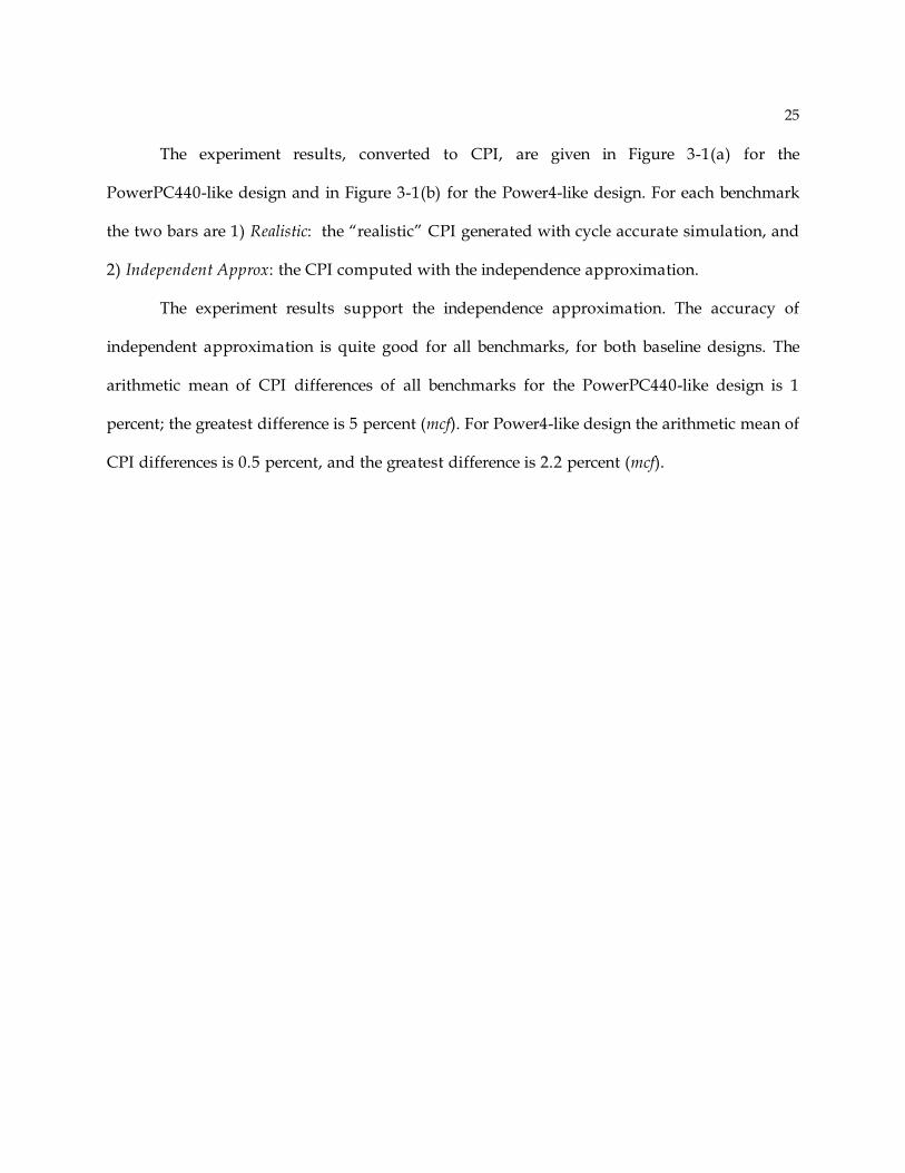
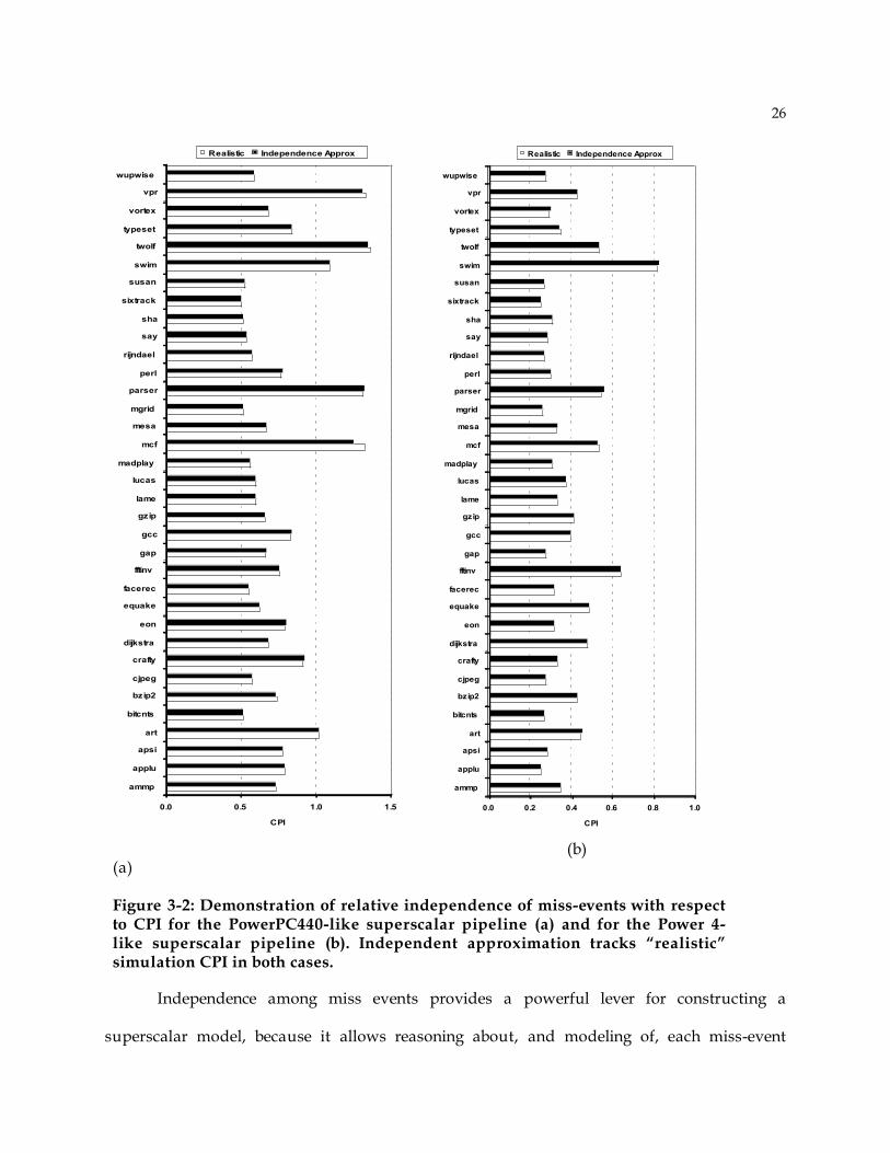
The experiment results, converted to CPI, are given in Figure 3-1(a) for the

PowerPC440-like design and in Figure 3-1(b) for the Power4-like design. For each benchmark

the two bars are 1) Realistic: the “realistic” CPI generated with cycle accurate simulation, and

2) Independent Approx: the CPI computed with the independence approximation.

The experiment results support the independence approximation. The accuracy of

independent approximation is quite good for all benchmarks, for both baseline designs. The

arithmetic mean of CPI differences of all benchmarks for the PowerPC440-like design is 1

percent; the greatest difference is 5 percent (mcf). For Power4-like design the arithmetic mean of

CPI differences is 0.5 percent, and the greatest difference is 2.2 percent (mcf).

26

0.0 0.5 1.0 1.5

ammp

applu

apsi

art

bitcnts

bzip2

cjpeg

crafty

dijkstra

eon

equake

facerec

fftinv

gap

gcc

gzip

lame

lucas

madplay

mcf

mesa

mgrid

parser

perl

rijndael

say

sha

sixtrack

susan

swim

twolf

typeset

vortex

vpr

wupwise

CPI

Realistic Independence Approx

(a) (b)

Figure 3-2: Demonstration of relative independence of miss-events with respect to CPI for the PowerPC440-like superscalar pipeline (a) and for the Power 4-like superscalar pipeline (b). Independent approximation tracks “realistic” simulation CPI in both cases.

Independence among miss events provides a powerful lever for constructing a

superscalar model, because it allows reasoning about, and modeling of, each miss-event

0.0 0.2 0.4 0.6 0.8 1.0

ammp

applu

apsi

art

bitcnts

bzip2

cjpeg

crafty

dijkstra

eon

equake

facerec

fftinv

gap

gcc

gzip

lame

lucas

madplay

mcf

mesa

mgrid

parser

perl

rijndael

say

sha

sixtrack

susan

swim

twolf

typeset

vortex

vpr

wupwise

CPI

Realistic Independence Approx

27

category more-or-less in isolation. Individual miss-events within the same category, however,

are not necessarily independent; at least this can not be inferred from the above experiments.

This implies that “bursts” of miss-events of a given type may have to be modeled; for

example, when a burst of branch mispredictions or cache misses cluster together closely in

time.

In the remainder of this chapter an analytical CPI model is developed that contains the

following components:

1. A method for determining the ideal, sustainable performance (CPI), in terms of

implementation-independent dynamic instruction stream statistics and microarchitecture

parameters.

2. Methods for estimating the penalties for branch mispredictions, instruction cache misses,

and data cache misses, in terms of the microarchitecture parameters.

3. A method for taking miss-event rates and combining them with the CPI under ideal

conditions and the penalties for performance degrading events to arrive at overall CPI

estimates.

Along the way, the new model is used to derive insights into the operation of superscalar

processors. These insights are also verified with a comparison to a more accurate cycle-

accurate simulation model. Finally, the complete CPI model is validated against overall CPI

performance generated with cycle-accurate simulation.

3.2 Top-level CPI Model

For reasoning about superscalar processor operation, a schematic representation shown

in Figure 3-3 is used. The Ifetch unit is capable of providing a never-ending supply of

instructions. Instructions pass through the front-end pipeline, experiencing lfe cycle delay,

28

before being dispatched into both the issue window and the re-order buffer. The fetch width,

pipeline width, dispatch width, retire width, and maximum issue width are all characterized

with parameter I. Instructions issue at a rate determined by the i-W characteristic, i.e. a function

that determines the number of instructions that issue in a clock cycle, given the number of

instructions in the window (or reorder buffer).

At the time instructions are fetched, there is a probability, mbr, that there is a branch

misprediction. If so, the fetching of useful instructions is stopped. Fetching of useful

instructions resumes only when all good instructions in the processor have issued. This model

assumes that the mispredicted branch is the oldest correct-path instruction to issue because of

the misprediction. It will become evident in Section 3.4 that the assumption is valid for a first-

order CPI model.

Also at the time instructions are fetched, there is a probability, mil1, that there is a miss

in the level-1 instruction cache and a probability mil2 that there is an instruction miss in the

level-2 cache. If there is a miss, instruction fetching is stopped, and it resumes only after

instructions can be fetched from the L2 cache after ll2 cycles, or from memory after lmm cycles.

When there is a long data cache miss (L2 miss) the retirement of instructions from the reorder

buffer is stopped. After a miss delay of lmm cycles, data returns from memory, and retirement

is re-started. Short data cache misses (L1 misses) are modeled as if they are handled by long

latency functional units.

29

If e tc h

stop

start

empty

&stop

start

mispredictSize

pipe

Icache miss

win_siz e

rob_ size

Lon g

Dcache miss

stop

start

IW

characteristic

i i i i i

i

< i_

l

lfe

lmm

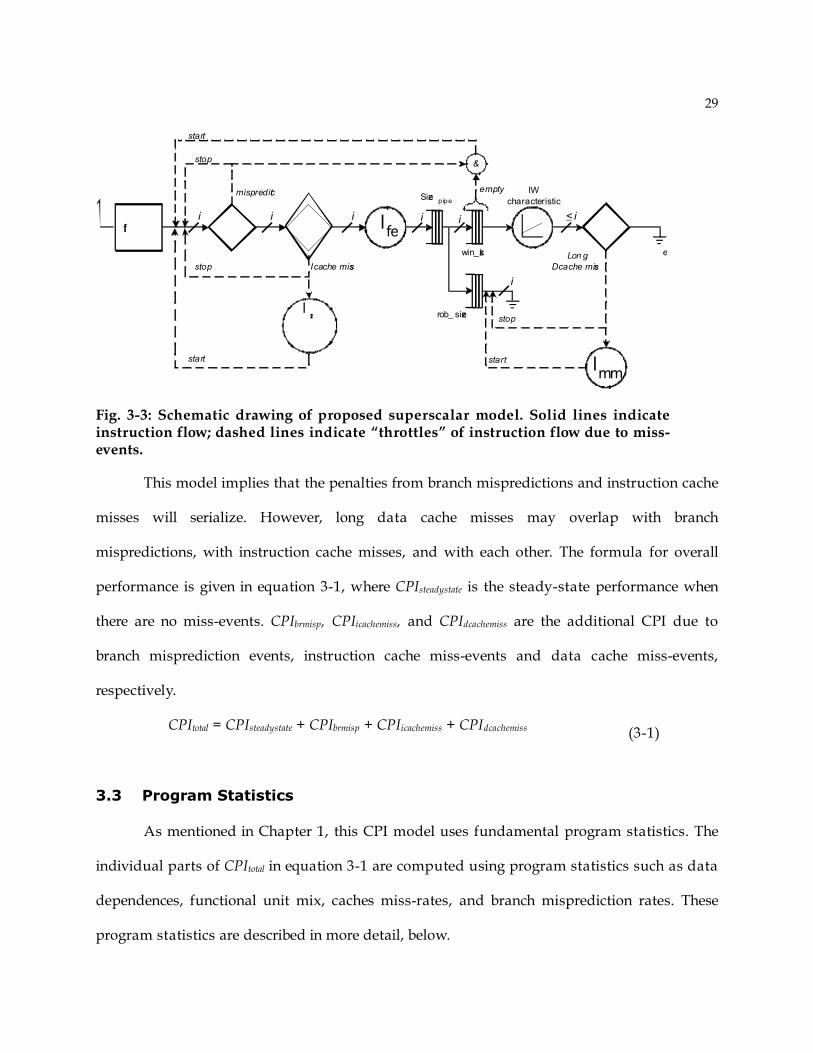
Fig. 3-3: Schematic drawing of proposed superscalar model. Solid lines indicate instruction flow; dashed lines indicate “throttles” of instruction flow due to miss-events.

This model implies that the penalties from branch mispredictions and instruction cache

misses will serialize. However, long data cache misses may overlap with branch

mispredictions, with instruction cache misses, and with each other. The formula for overall

performance is given in equation 3-1, where CPIsteadystate is the steady-state performance when

there are no miss-events. CPIbrmisp, CPIicachemiss, and CPIdcachemiss are the additional CPI due to

branch misprediction events, instruction cache miss-events and data cache miss-events,

respectively.

CPItotal = CPIsteadystate + CPIbrmisp + CPIicachemiss + CPIdcachemiss (3-1)

3.3 Program Statistics

As mentioned in Chapter 1, this CPI model uses fundamental program statistics. The

individual parts of CPItotal in equation 3-1 are computed using program statistics such as data

dependences, functional unit mix, caches miss-rates, and branch misprediction rates. These

program statistics are described in more detail, below.

30

• Data dependences are modeled by measuring the length of the longest dependence chain

for a sequence of W dynamic instructions. The parameter W is varied from 1 to 1024.

• Functional unit mix is the fraction of the executed instructions that use each of the

functional unit types (for example, an integer ALU or data cache port).

• Cache miss-rate is the number of instructions that miss in the cache divided by total

number of instructions in the program. Cache miss rates are measured for the L1 instruction

cache and denoted as mil1, the L1 data cache and denoted as mdl1, and for the unified L2

cache. The L2 miss rate is decomposed into the instruction miss rate, denoted as mil2, and

the data miss rate, denoted as mdl2. The miss rates are determined for the set of caches in the

component database.

• Branch misprediction rate, denoted as mbr, is number of branches that are mispredicted

divided by total number of instructions in the program. The value for mbr is measured for all

branch predictors in the component database.

• Load statistics measure the distribution of independent L2 cache load misses, fldm(S), given

S dynamic instructions following a load miss. The parameter S is varied over all available

reorder buffer sizes in the component database. This statistic is measured for all L2 caches

in the component database.

The aforementioned program statistics are collected with computationally simple

analysis of dynamic instruction trace of the target program(s). The time required by the trace-

driven simulators to analyze a trace of 100 million instructions with a single-threaded 1.8GHz

Pentium-4 machine is in Table 3-1. If longer traces are used, these times will grow linearly with

trace length. As indicated in the table, a single trace-driven simulation collects the data

dependence statistics, function unit mix, and the load statistics.

31

Table 3-1: Time required to generate program statistics for 100M instructions on a 1.8GHz single threaded Pentium-4 machine.

Program Statistic Time per 100M instructions

Data dependences, Func. Unit mix,

Load stats.

1.8 min

Cache miss rates 36 seconds per cache configuration

Branch misprediction rates 2 mins per predictor configuration

Sections 3.3 to 3.6 develop methods to compute the individual parts of the overall CPI

using these program statistics. Section 3.3 focus on the iW Characteristic model. Sections 3.4,

3.5, and 3.6 develop methods for computing penalties due to branch mispredictions,

instruction cache misses, and data cache misses, respectively.

3.4 The iW Characteristic

The iW characteristic is important both for determining the ideal, steady-state

performance level and for estimating miss-event penalties. The iW characteristic expresses the

relationship between the number of in-flight instructions in the processor, denoted as W, and

the number of instructions that will issue (on average), denoted as i. Average issue rate is a

function of number of in-flight instructions, the instruction dependence structure of the

program, and the processor’s issue width.

The iW Characteristic model is developed in three steps. First, the average issue rate is

modeled as a function of in-flight instructions assuming an unbounded issue width. Second,

the effect of a bounded issue width on the average issue rate is modeled. Third, the limitation

on the average issue rate imposed by taken branches is modeled.

32

3.4.1 Unbounded Issue Width

At the top-level, a processor can be divided into two parts: the instruction fetch

mechanism, and the instruction execution mechanism. Assuming instruction fetch is able to

deliver instructions at the rate demanded by the instruction execution, instruction execution

will determine the instruction throughput. In current microprocessors, the reorder buffer holds

all in-flight instructions in the instruction execution mechanism. Because instructions enter and

exit the reorder buffer in the program order, the critical path of the instructions in the reorder

buffer determines the performance under ideal conditions (no miss events). Therefore, the

average issue-rate assuming unbounded issue width is modeled as

i = W/(lavg*K� (W)) (3-2)

where W is the reorder buffer (window) size, K� (W) is the length of the average critical path

(measured as instructions) for W consecutive dynamic instructions and lavg is the average

instruction execution latency (also measured in cycles). The term lavg*K� (W) therefore computes

the critical path in terms of cycles; that is, the number of cycles necessary to retire W

instructions from the reorder buffer.

As mentioned earlier in Chapter 2, Michaud, et al. [32] observed a square-root

relationship between the window size (or reorder buffer size, in today’s terms) and the average

length of the longest critical path for the window-size instructions. Therefore, this chapter

develops iW Characteristic model that uses the distribution of the critical path lengths for

window sizes ranging from one to 1024.

The critical path length distribution is modeled as the probability PK(K(W)=n), where

the random process K(W) gives the critical path for a sequence of W dynamic instructions. The

random process K(W) is measured with trace-driven analysis of dynamic instruction trace of

the program. The function K� (W) from equation 3-2 is then calculated using K(W) as

33

=! =" 1

( ( ( ) ))W

Knn P K W n . The parameter lavg is derived from function-unit mix of the target

program, as mentioned earlier in Section 3.1.

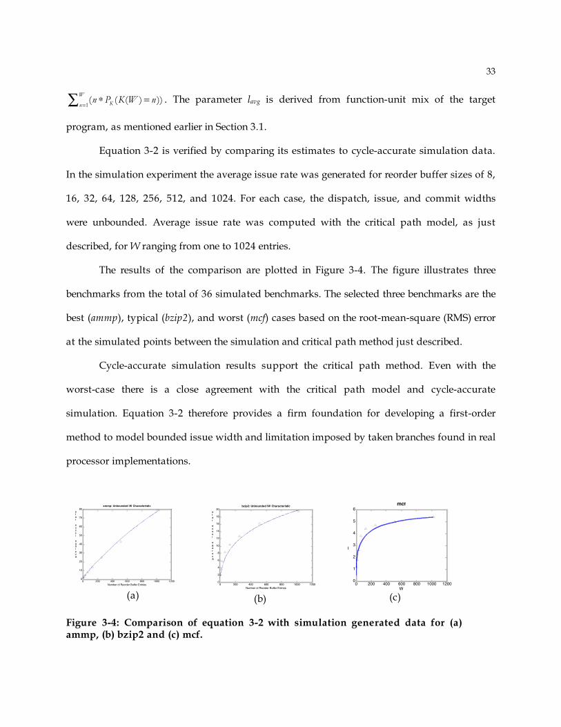
Equation 3-2 is verified by comparing its estimates to cycle-accurate simulation data.

In the simulation experiment the average issue rate was generated for reorder buffer sizes of 8,

16, 32, 64, 128, 256, 512, and 1024. For each case, the dispatch, issue, and commit widths

were unbounded. Average issue rate was computed with the critical path model, as just

described, for W ranging from one to 1024 entries.

The results of the comparison are plotted in Figure 3-4. The figure illustrates three

benchmarks from the total of 36 simulated benchmarks. The selected three benchmarks are the

best (ammp), typical (bzip2), and worst (mcf) cases based on the root-mean-square (RMS) error

at the simulated points between the simulation and critical path method just described.

Cycle-accurate simulation results support the critical path method. Even with the

worst-case there is a close agreement with the critical path model and cycle-accurate

simulation. Equation 3-2 therefore provides a firm foundation for developing a first-order

method to model bounded issue width and limitation imposed by taken branches found in real

processor implementations.

(a) (b) (c)

Figure 3-4: Comparison of equation 3-2 with simulation generated data for (a) ammp, (b) bzip2 and (c) mcf.

0 200 400 600 800 1000 12000

2

4

6

8

10

12

14

16

18

20bzip2: Unbounded IW Characteristic

Average issue rate

Number of Reorder Buffer Entries

0 200 400 600 800 1000 12000

10

20

30

40

50

60

70

80ammp: Unbounded IW Characteristic

Average issue rate

Number of Reorder Buffer Entries 0 200 400 600 800 1000 12000

1

2

3

4

5

6

mcf

I

W

34

3.4.2 Bounded Issue Width

When the maximum issue width is limited, as it would be in a superscalar processor,

then the iW curves change somewhat [46]. For example, Figure 3-5 shows the iW curves with

limited issue width for gcc on a log-log scale, generated with cycle-accurate simulation. The

limited issue width curves follow the unbounded issue width curves until the reorder buffer

size equals the issue width, and then they asymptotically approach the issue width limit; that

is, instruction issue saturates at the maximum rate.

Figure 3-5: IW Characteristic after bounding the issue width. Issue width of 2, 4, and 8 are shown.

The effect of issue width bound on the instruction throughput is modeled by first

computing the probabilities of instruction issues for the unbounded issue width case, using the

critical path model. Then, the instruction issue distribution is modified such that issue rates

greater than the issue width are truncated to the issue width bound. Finally, the average issue

rate for the bounded issue width case is computed as the expectation of the truncated

instruction issue probabilities.

Instruction issue probabilities are directly related to the critical path probabilities. Let

P’(i(W)=n) denote the probability of issuing n instructions in a cycle, where the random process

i(W) gives the number of instructions issuing in a cycle when there are W instructions in the

reorder buffer. Because i(W) = W/(K(W)*lavg) (equation 3-2), the following equality holds:

gcc

0

1

2

3

4

5

0 1 2 3 4 5 6 7

log2(W)

log2(I)

unlimited

iss-w idth=4

iss-w idth=2

iss-w idth=8

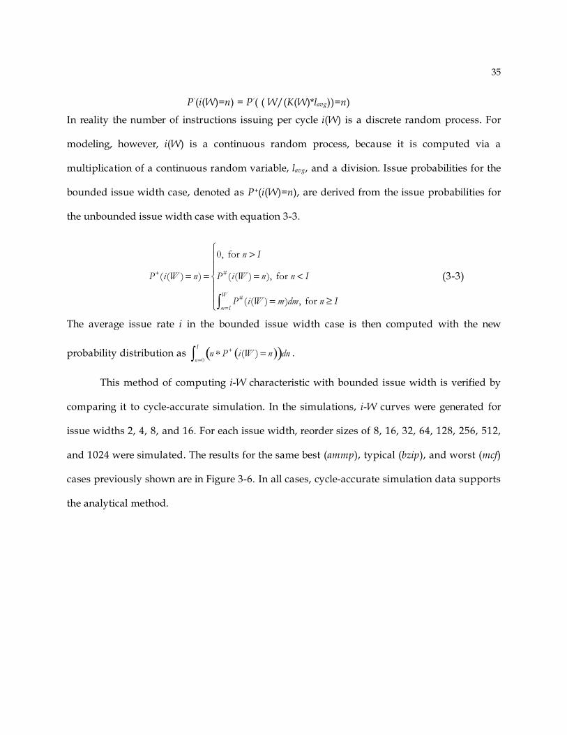
35

P’(i(W)=n) = P’( ( W/(K(W)*lavg))=n)

In reality the number of instructions issuing per cycle i(W) is a discrete random process. For

modeling, however, i(W) is a continuous random process, because it is computed via a

multiplication of a continuous random variable, lavg, and a division. Issue probabilities for the

bounded issue width case, denoted as P+(i(W)=n), are derived from the issue probabilities for

the unbounded issue width case with equation 3-3.

+

=

!>"

"= = = <#

""

= $%&

#

#

0, for

( ( ) ) ( ( ) ), for

( ( ) ) , for W

m I

n I

P i W n P i W n n I

P i W m dm n I

(3-3)

The average issue rate i in the bounded issue width case is then computed with the new

probability distribution as ( )( )+

=! =" 0

( )I

n

n P i W n dn .

This method of computing i-W characteristic with bounded issue width is verified by

comparing it to cycle-accurate simulation. In the simulations, i-W curves were generated for

issue widths 2, 4, 8, and 16. For each issue width, reorder sizes of 8, 16, 32, 64, 128, 256, 512,

and 1024 were simulated. The results for the same best (ammp), typical (bzip), and worst (mcf)

cases previously shown are in Figure 3-6. In all cases, cycle-accurate simulation data supports

the analytical method.

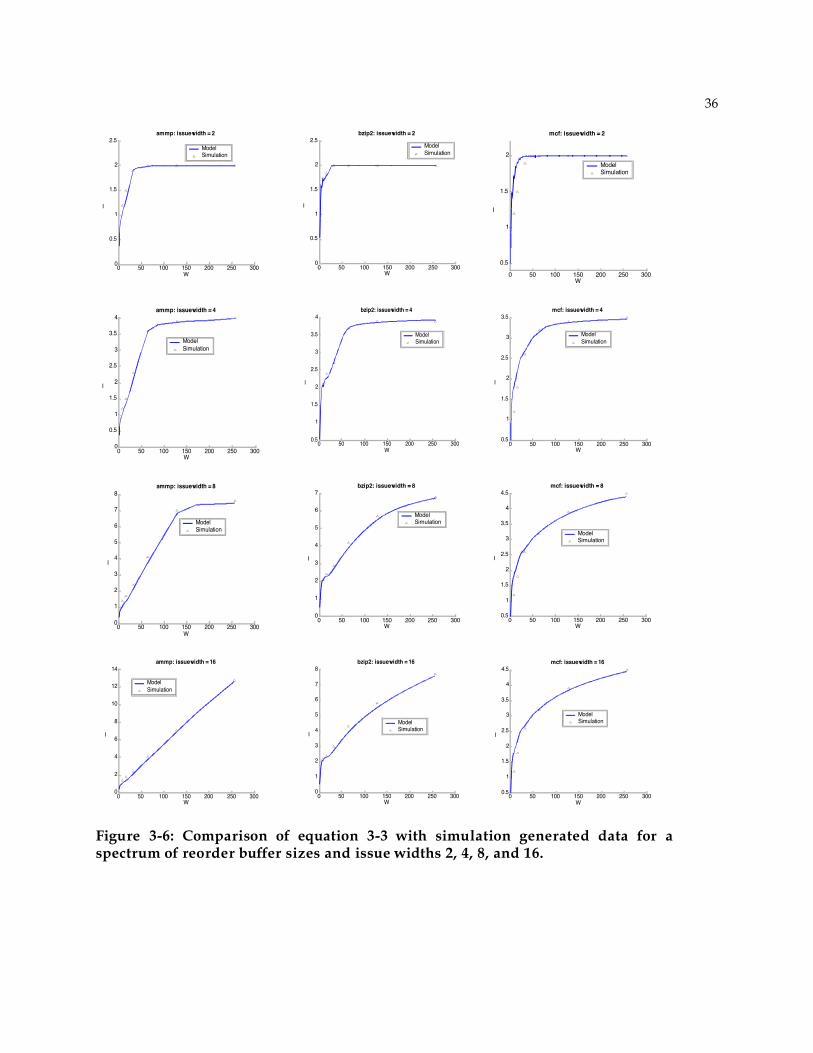
36

0 50 100 150 200 250 3000

0.5

1

1.5

2

2.5

ammp: issuewidth = 2

I

W

Model

Simulation

0 50 100 150 200 250 3000

0.5

1

1.5

2

2.5

bzip2: issuewidth = 2

I

W

Model

Simulation

0 50 100 150 200 250 300

0.5

1

1.5

2

mcf: issuewidth = 2

I

W

Model

Simulation

0 50 100 150 200 250 3000

0.5

1

1.5

2

2.5

3

3.5

4

ammp: issuewidth = 4

I

W

Model

Simulation

0 50 100 150 200 250 300

0.5

1

1.5

2

2.5

3

3.5

4

bzip2: issuewidth = 4

I

W

Model

Simulation

0 50 100 150 200 250 300

0.5

1

1.5

2

2.5

3

3.5

mcf: issuewidth = 4

I

W

Model

Simulation

0 50 100 150 200 250 3000

1

2

3

4

5

6

7

8

ammp: issuewidth = 8

I

W

Model

Simulation

0 50 100 150 200 250 3000

1

2

3

4

5

6

7

bzip2: issuewidth = 8

I

W

Model

Simulation

0 50 100 150 200 250 300

0.5

1

1.5

2

2.5

3

3.5

4

4.5

mcf: issuewidth = 8

I

W

Model

Simulation

0 50 100 150 200 250 3000

2

4

6

8

10

12

14

ammp: issuewidth = 16

I

W

Model

Simulation

0 50 100 150 200 250 3000

1

2

3

4

5

6

7

8

bzip2: issuewidth = 16

I

W

Model

Simulation

0 50 100 150 200 250 300

0.5

1

1.5

2

2.5

3

3.5

4

4.5

mcf: issuewidth = 16

I

W

Model

Simulation

Figure 3-6: Comparison of equation 3-3 with simulation generated data for a spectrum of reorder buffer sizes and issue widths 2, 4, 8, and 16.

37

3.4.3 Modeling Taken Branches

Thus far, the instruction fetch mechanism is assumed to be ideal; every fetch brings into

the processor as many instructions as instruction execution demands. In reality, however,

taken branches interrupt instruction fetching, and consequently, they set an upper limit on the

average issue rate that can be achieved. Taken branches essentially upper bound the issue-rate,

similar to the bound imposed by the issue width. Note that here a fetch unit that stops at

taken branches is assumed. Aggressive fetch units that fetch beyond taken branches have been

proposed [47]. The performance impact of those aggressive fetch units can be modeled by

simply using the average issue rate modeled developed thus far and ignoring the fetch

inefficiency term introduced in this section.

To model the upper bound on issue rate because of taken branches, the following three

new parameters are defined. Let ptbr stand for the probability of encountering a taken branch in

the target program. Let F denote the fetch width of the instruction fetch mechanism. And, let f

be the number of instructions brought into the processor, on average, after every fetch. The

average fetch rate f is then computed with equation 3-4, below.

( )( )

( )( )!

=

" #" #= $ ! + $ !% &' (' ()

1

1

1 1

Fl F

tbr tbr tbr

l

f l p p F p (3-4)

The geometric-series term ( )( )!

=" !#

1

1[ 1 ]

F l

tbr tbrll p p in equation 3-4 models the

possibilities that l instructions can be fetched in a single access and the last instruction is a

taken branch. The other term ( )( )! "1F

tbrF p models the case where F instructions can be

obtained in a single fetch when none of the F instructions are taken branches. To make

subsequent modeling easier a new term called the fetch efficiency is introduced. The fetch

efficiency is denoted by � F, and is defined as ratio of the average fetch rate and the fetch

width. Mathematically, fetch efficiency is computed as: � F = f÷F.

38

In this dissertation the fetch width and issue width are set equal. (The methods

presented however can accommodate independently determined fetch and issue widths.) Issue

probabilities are then calculated by substituting I in equation 3-3 with � F×I. The modified

equation for issue probabilities is given below as equation 3-5.

( )

( )

( ) ( )

( ) ( )( )!

!

!

!

+

+

= "

#> "$

$$= = = < "%

$$

= & "$'(

0, for

( ) ( ) , for

( ) , for F

F

F

W

Fm I

n I

P i W n P i W n n I

P i W m dm n I

(3-5)

The average issue rate i is then computed as the expectation using the new probabilities. This

is expressed mathematically in equation 3-6.

( )( )( )! "

== " =# 0

( )FI

n

i n P i W n dn (3-6)

Equation 3-6 is verified by comparing the i-W curves it computes to the i-W curves

generated with cycle-accurate simulations. In the model and simulation the fetch width the

issue width are set (to be) equal to each other. Cycle-accurate simulation is performed for

issue-widths of 2, 4, 8, and 16. For each issue width, average issue rate for reorder buffer sizes

of 8, 16, 32, 64, 128, 256, and 512 is generated.

The results of the comparison are plotted in Figure 3-7. In the figure, the same best,

typical, and worst cases are shown. The analytical model tracks simulation generated data for

issue widths and reorder buffer sizes examined. Overall, cycle-accurate simulation data

supports equation 3-6.

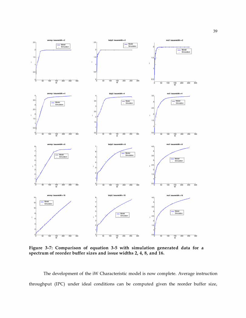
39

0 50 100 150 200 250 3000

0.5

1

1.5

2

2.5

ammp: issuewidth = 2

I

W

Model

Simulation

0 50 100 150 200 250 3000

0.5

1

1.5

2

2.5

bzip2: issuewidth = 2

I

W

Model

Simulation

0 50 100 150 200 250 300

0.5

1

1.5

2

mcf: issuewidth = 2

I

W

Model

Simulation

0 50 100 150 200 250 3000

0.5

1

1.5

2

2.5

3

3.5

4

ammp: issuewidth = 4

I

W

Model

Simulation

0 50 100 150 200 250 300

0.5

1

1.5

2

2.5

3

3.5

4

bzip2: issuewidth = 4

I

W

Model

Simulation

0 50 100 150 200 250 300

0.5

1

1.5

2

2.5

3

3.5

mcf: issuewidth = 4

I

W

Model

Simulation

0 50 100 150 200 250 3000

1

2

3

4

5

6

7

8

ammp: issuewidth = 8

I

W

Model

Simulation

0 50 100 150 200 250 3000

1

2

3

4

5

6

7

bzip2: issuewidth = 8

I

W

Model

Simulation

0 50 100 150 200 250 300

0.5

1

1.5

2

2.5

3

3.5

4

4.5

mcf: issuewidth = 8

I

W

Model

Simulation

0 50 100 150 200 250 3000

2

4

6

8

10

12

14

ammp: issuewidth = 16

I

W

Model

Simulation

0 50 100 150 200 250 3000

1

2

3

4

5

6

7

8

bzip2: issuewidth = 16

I

W

Model

Simulation

0 50 100 150 200 250 300

0.5

1

1.5

2

2.5

3

3.5

4

4.5

mcf: issuewidth = 16

I

W

Model

Simulation

Figure 3-7: Comparison of equation 3-5 with simulation generated data for a spectrum of reorder buffer sizes and issue widths 2, 4, 8, and 16.

The development of the iW Characteristic model is now complete. Average instruction

throughput (IPC) under ideal conditions can be computed given the reorder buffer size,

40

instruction mix, issue width, and taken branch probability. CPIsteadystate from equation 3-1 is

simply the inverse of i the IPC from equation 3-6.

As mentioned earlier, the iW characteristic plays a central role in determining additional

cycles (performance loss) due to miss-events. Additional cycles for miss-events are computed

by first determining the clock cycle penalty for each type of miss-event, counting the numbers

miss-events of each type, then multiplying the two. The three subsequent sections develop

first-order models for computing miss-event penalties using the iW Characteristic. Section 3.4

develops the branch misprediction penalty model. Section 3.5 focuses on instruction cache

misses. Section 3.6 models the data cache miss penalty.

The miss-event counts are generated with simple trace-driven simulations. Sections 3.4,

3.5, and 3.6 that follow develop first-order models for computing clock cycle penalties for

branch mispredictions, instruction cache misses, and long data cache misses, respectively.

3.5 Branch Misprediction Penalty

To model the branch misprediction penalty, the iW Characteristic and the schematic in

Figure 3-3 is used. First a single branch misprediction is considered in isolation. Then, the effect

of bursts of branch mispredictions is modeled.

The transient for a single isolated branch misprediction is shown in Figure 3-8. Initially,

the processor is issuing instructions at the steady-state IPC. Then a mispredicted branch

causes fetching of useful instructions to stop. Eventually, the mispredicted branch is

dispatched and enters the reorder buffer. At this point, no more useful instructions are

dispatched until the mispredicted branch is resolved. If the instructions issue in oldest-first

priority, none of the miss-speculated instructions will inhibit any of the useful instructions

from issuing. Consequently, only useful instructions need to be considered.

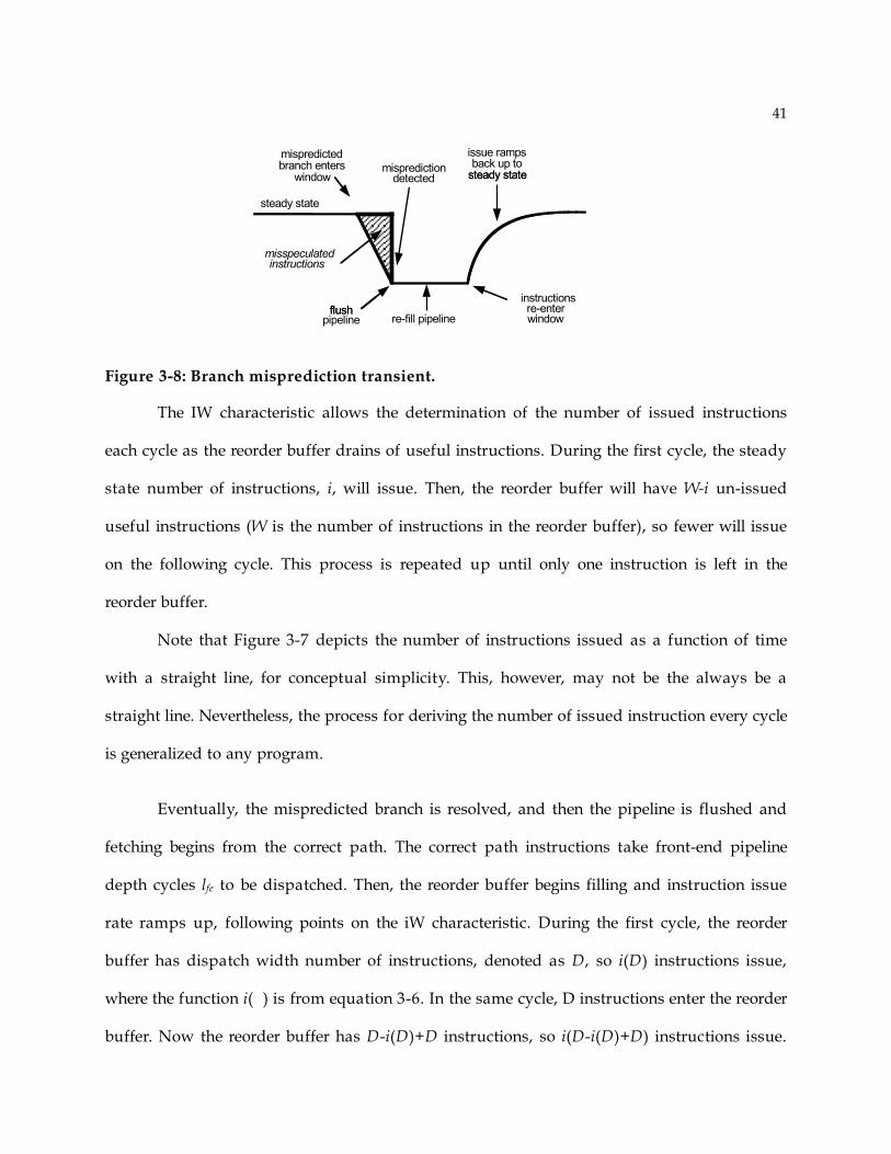
41

Figure 3-8: Branch misprediction transient.

The IW characteristic allows the determination of the number of issued instructions

each cycle as the reorder buffer drains of useful instructions. During the first cycle, the steady

state number of instructions, i, will issue. Then, the reorder buffer will have W-i un-issued

useful instructions (W is the number of instructions in the reorder buffer), so fewer will issue

on the following cycle. This process is repeated up until only one instruction is left in the

reorder buffer.

Note that Figure 3-7 depicts the number of instructions issued as a function of time

with a straight line, for conceptual simplicity. This, however, may not be the always be a

straight line. Nevertheless, the process for deriving the number of issued instruction every cycle

is generalized to any program.

Eventually, the mispredicted branch is resolved, and then the pipeline is flushed and

fetching begins from the correct path. The correct path instructions take front-end pipeline

depth cycles lfe to be dispatched. Then, the reorder buffer begins filling and instruction issue

rate ramps up, following points on the iW characteristic. During the first cycle, the reorder

buffer has dispatch width number of instructions, denoted as D, so i(D) instructions issue,

where the function i( ) is from equation 3-6. In the same cycle, D instructions enter the reorder

buffer. Now the reorder buffer has D-i(D)+D instructions, so i(D-i(D)+D) instructions issue.

steady state

flushflushpipeline re-fill pipeline

mispredictiondetected

misspeculatedinstructions

back up tosteady state

issue ramps

steady state

mispredictedbranch enters

window

instructionsre-enterwindow

42

This process continues up until the average issue rate reaches the steady-state IPC. The ramp-

up curve rises quickly at first, then more slowly as instructions are issued while the reorder

buffer is filling (like filling a “leaky bucket” [32]).

This model assumes that the mispredicted branch is the oldest unissued instruction in

the reorder buffer at the time it is resolved. Data from cycle accurate simulation supports this

assumption. A cycle-accurate simulation experiment was conducted with a realistic branch

predictor and ideal caches. The number of un-issued correct-path instructions were recorded

whenever a mispredicted branch issued.

The results are in the histogram plotted in Figure 3-9. The x-axis of the figure has the

number of unissued correct-path instruction left in the reorder buffer when a mispredicted

branch is resolved. The y-axis has the frequency in terms of the number of benchmarks of

having unissued correct-path instructions in the reorder buffer, plotted with the results from

both baseline design simulations.

The histogram is clearly skewed towards small values. The mode of the histogram is

three, while its mean is six. The benchmark sha is an outlier with 23 un-issued instructions left

in the reorder buffer. Clearly, the number of un-issued instructions left in the reorder buffer is a

function of benchmark. In general, however, only a few un-issued correct-path instructions are

left in the reorder buffer. For a first-order estimate, this dissertation takes the upper bound on

branch misprediction penalty, by modeling the mispredicted branch as the oldest correct-path

instruction to be issued.

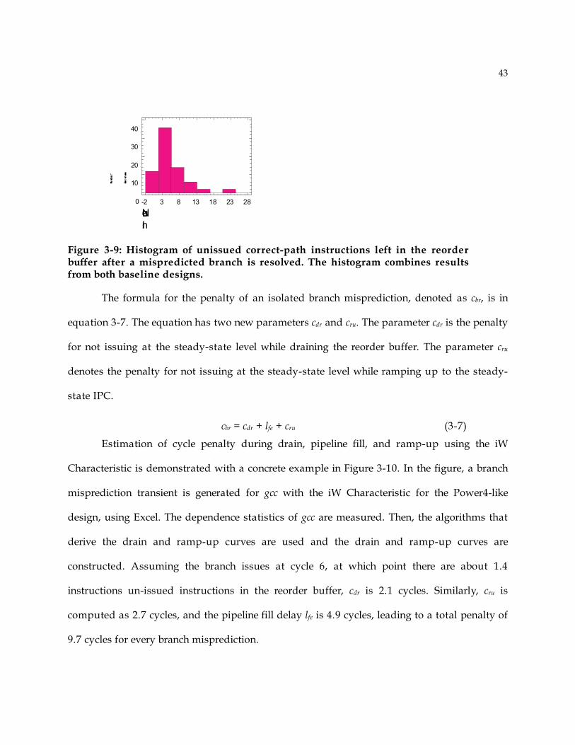
43

-2 3 8 13 18 23 28

Nu m be r of Uniss ue d

In s tr uctions

0

10

20

30

40

Figure 3-9: Histogram of unissued correct-path instructions left in the reorder buffer after a mispredicted branch is resolved. The histogram combines results from both baseline designs.

The formula for the penalty of an isolated branch misprediction, denoted as cbr, is in

equation 3-7. The equation has two new parameters cdr and cru. The parameter cdr is the penalty

for not issuing at the steady-state level while draining the reorder buffer. The parameter cru

denotes the penalty for not issuing at the steady-state level while ramping up to the steady-

state IPC.

cbr = cdr + lfe + cru (3-7)

Estimation of cycle penalty during drain, pipeline fill, and ramp-up using the iW

Characteristic is demonstrated with a concrete example in Figure 3-10. In the figure, a branch

misprediction transient is generated for gcc with the iW Characteristic for the Power4-like

design, using Excel. The dependence statistics of gcc are measured. Then, the algorithms that

derive the drain and ramp-up curves are used and the drain and ramp-up curves are

constructed. Assuming the branch issues at cycle 6, at which point there are about 1.4

instructions un-issued instructions in the reorder buffer, cdr is 2.1 cycles. Similarly, cru is

computed as 2.7 cycles, and the pipeline fill delay lfe is 4.9 cycles, leading to a total penalty of

9.7 cycles for every branch misprediction.

44

Figure 3-10: Transient curve for an isolated branch misprediction

The penalty computation method just described sets an upper bound on the branch

misprediction penalty, because it assumes mispredictions occur in isolation. For bursts of

branch mispredictions, the drain and ramp-up penalties “bracket” a series of pipeline fills,

each of which delivers a small number of useful instructions. In the extreme case of n

consecutive branch mispredictions, the formula for cbr is given in equation 3-8.

cbr = lfe + [(cdr + cru)/n] (3-8)

In the limit, n goes to infinity and cbr is simply lfe cycles. The depth of the front-end pipeline is

then a lower bound on the branch misprediction penalty.

Depending on the amount of clustering of branch mispredictions, the branch

misprediction penalty will be between the upper bound and the lower bound penalty. One way

to compute the penalty is to first measure branch misprediction clustering for every

combination of branch predictor and superscalar microarchitecture. Then, a polynomial will

express the misprediction penalty using data on branch misprediction clustering as its

coefficients.

An alternative method is to simply use the mid-point of the upper and lower bounds

with the formula in equation 3-9, below.

cbr = lfe + (cdr + cru)/2 (3-9)

0

1

2

3

4

0 2 4 6 8 10 12 14 16 18 20 22 24 26 28 30

clock cycle

instr

ucti

on

s

issu

ed

drain: 2.1 cycles

front end pipeline: 4.9 cyclesramp up: 2.7 cycles

45

Computing the mid-point of the extreme cases has two key advantages over the polynomial

method: 1) mid-point computation requires computationally and conceptually simple

summation of upper bound and lower bound followed by a division by two, and 2) mid-point

value guarantees that the difference between the analytical model derived penalty and the

actual penalty, on average, is no more than half the difference between the two extremes.

Equation 3-9 gives the following insight regarding branch mispredictions: the branch

misprediction penalty can be significantly greater than the (often assumed) front-end pipeline depth.

For the example five-stage front end, the total penalty can be twice the front-end pipeline

depth.

To validate this part of the CPI model, each baseline processor is simulated with two

front-end pipeline lengths. PowerPC440-like baseline is simulated with five and ten front-end

stages, while the Power4-like baseline is simulated with 11 and 16 front-end stages. In one set

of simulations, the designs are simulated with ideal instruction and data caches and realistic

branch predictors. In a second set of simulations, the branch predictor is ideal. Then, using the

results of these two sets of simulations, the penalty for every branch misprediction on average

is computed. This simulation generated penalty is compared with the penalty computed with

equation 3-8 and the upper and lower bounds set with equations 3-7 and 3-6, respectively.

The results are plotted in Figure 3-11 for PowerPC440-like baseline and in Figure 3-12

for Power4-like baseline. The penalty for a branch misprediction, averaged over all branch

mispredictions, is on the y-axis.

For the PowerPC440-like baseline, Figure 3-11 (a) shows the branch misprediction

penalty for five front-end pipeline stages. The penalty is between the model derived lower and

upper bounds. The penalty is also much greater than the front-end pipeline depth. Similar to

46

the five-stage front-end, with a ten stage front-end pipeline (Figure 3-11(b)), the penalty for a

branch misprediction is greater than ten cycles and within the range derived by the model.

The results for the Power4-like baseline are in Figure 3-12 (a) and (b). Figure 3-12(a)

has the results for 11 front-end pipeline stages and Figure 3-12(b) has the results for 16 front-

end pipeline stages. The trends are the same as those for the PowerPC440-like design. The

misprediction penalty is greater than the front-end pipeline length and always within the range

predicted by equations 3-6 and 3-7. With the mid-point approximation the average difference

between analytical model and cycle-accurate simulation estimates is always less than 34

percent (madplay), and 17 percent on average.

Modeling of branch misprediction is one of the most difficult parts of this model, for

obtaining a high absolute accuracy. It is the weakest link in the model presented in this

dissertation. This weakness however has been eliminated with a new approach called Interval

Analysis[48]. Searching for Pareto-optimal design however relies more on relative accuracy

rather than absolute accuracy. As shall be evident in Chapter 5, the model presented with mid-

point approximation finds the Pareto-optimal superscalar designs.

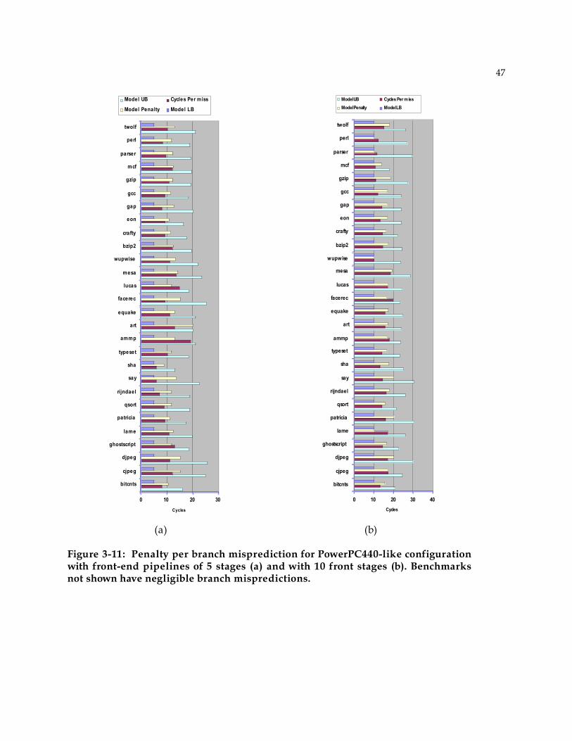
47

(a) (b)

Figure 3-11: Penalty per branch misprediction for PowerPC440-like configuration with front-end pipelines of 5 stages (a) and with 10 front stages (b). Benchmarks not shown have negligible branch mispredictions.

0 10 20 30

bitcnts

cjpeg

djpeg

ghostscript

lame

patricia

qsort

rijndael

say

sha

typeset

ammp

art

equake

facerec

lucas

mesa

wupwise

bzip2

crafty

eon

gap

gcc

gzip

mcf

parser

perl

twolf

Cycles

Model UB Cycles Per miss

Model Penalty Model LB

0 10 20 30 40

bitcnts

cjpeg

djpeg

ghostscript

lame

patricia

qsort

rijndael

say

sha

typeset

ammp

art

equake

facerec

lucas

mesa

wupwise

bzip2

crafty

eon

gap

gcc

gzip

mcf

parser

perl

twolf

Cycles

Model UB Cycles Per miss

Model Penalty Model LB

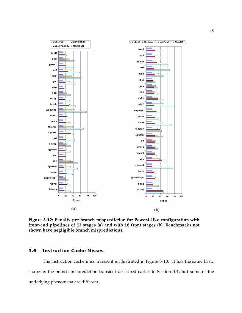
48

(a) (b)

Figure 3-12: Penalty per branch misprediction for Power4-like configuration with front-end pipelines of 11 stages (a) and with 16 front stages (b). Benchmarks not shown have negligible branch mispredictions.

3.6 Instruction Cache Misses

The instruction cache miss transient is illustrated in Figure 3-13. It has the same basic

shape as the branch misprediction transient described earlier in Section 3.4, but some of the

underlying phenomena are different.

0 20 40 60 80 100

bitcnts

cjpeg

ghostscript

lame

rijndael

sha

typeset

ammp

art

equake

facerec

lucas

mesa

wupwise

bzip2

crafty

eon

gap

gcc

gzip

mcf

parser

perl

twolf

Cycles

M odel UB Simulation M odel Penalty M odel LB

0 20 40 60 80 100

bitcnts

cjpeg

ghostscript

lame

rijndael

say

sha

typeset

ammp

art

equake

facerec

lucas

mesa

wupwise

bzip2

crafty

eon

gap

gcc

gzip

mcf

parser

perl

twolf

Cycles

Model UB Simulation

Model Penalty Model LB

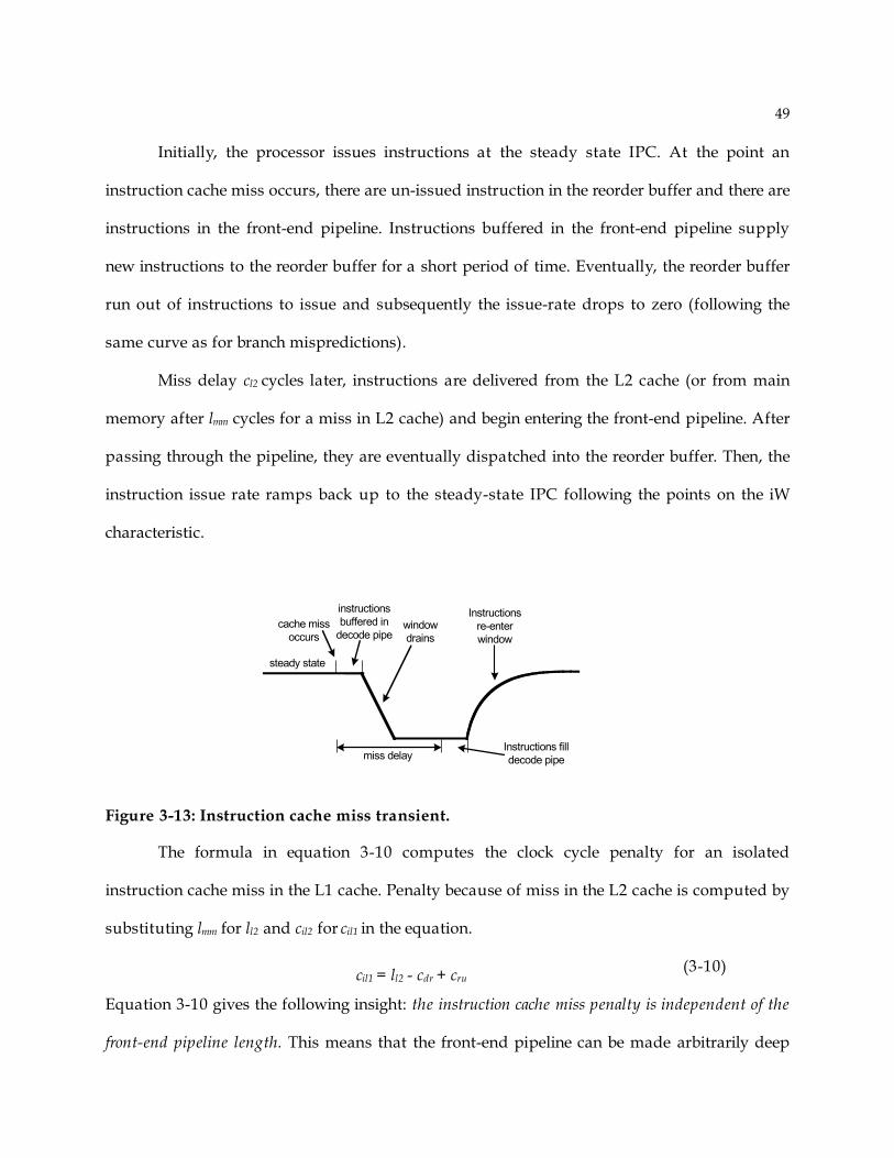
49

Initially, the processor issues instructions at the steady state IPC. At the point an

instruction cache miss occurs, there are un-issued instruction in the reorder buffer and there are

instructions in the front-end pipeline. Instructions buffered in the front-end pipeline supply

new instructions to the reorder buffer for a short period of time. Eventually, the reorder buffer

run out of instructions to issue and subsequently the issue-rate drops to zero (following the

same curve as for branch mispredictions).

Miss delay cl2 cycles later, instructions are delivered from the L2 cache (or from main

memory after lmm cycles for a miss in L2 cache) and begin entering the front-end pipeline. After

passing through the pipeline, they are eventually dispatched into the reorder buffer. Then, the

instruction issue rate ramps back up to the steady-state IPC following the points on the iW

characteristic.

Figure 3-13: Instruction cache miss transient.

The formula in equation 3-10 computes the clock cycle penalty for an isolated

instruction cache miss in the L1 cache. Penalty because of miss in the L2 cache is computed by

substituting lmm for ll2 and cil2 for cil1 in the equation.

cil1 = ll2 - cdr + cru (3-10)

Equation 3-10 gives the following insight: the instruction cache miss penalty is independent of the

front-end pipeline length. This means that the front-end pipeline can be made arbitrarily deep

steady state

miss delay

window

drains

Instructions

re-enter

window

cache miss

occurs

Instructions fill

decode pipe

instructions

buffered in

decode pipe

50

without affecting the instruction cache miss penalty. Equation 3-10 also indicates that the cdr

and cru offset each other (in contrast to the case for branch mispredictions where they add).

Because the drain and ramp-up penalties are derived from the same iW curve, the two penalty

are about the same, so their effects cancel. Consequently, the total instruction cache miss penalty

is approximately equal to the L2 cache (or main memory) latency.

If there are n consecutive instruction cache misses in a burst, then the formula for cil1 is

slightly modified as in equation 3-11, below.

cil1 = ll2 + [(cdr – cru)/n] (3-11)

Because cdr and cru offset each other (and this number is further diminished when divided by

n), equation 3-11 leads to the observation that an instruction cache miss yields the same penalty

regardless of whether it is isolated or is part of a burst of misses. Consequently, instruction cache

miss penalty is modeled by its miss delay. So, the penalty for a miss in the L1 cache and hit in

the L2 cache is just ll2 cycles, and similarly the penalty for a miss in the L2 cache is lmm cycles.

To confirm the above observations, the baseline processors are simulated as before,

with five and ten front-end pipeline stages for PowerPC440-like design and with 11 and 15

front-end pipeline stages for Power4-like design. The branch predictors and data caches are

ideal, but a non-ideal 4K 4-way set associative instruction cache with 128 byte cache lines is

modeled. The instruction cache miss delay ll2 (L2 access delay) is set at 10 cycles. The same

processors with ideal instruction caches are also simulated, and the average penalty per

instruction cache miss is computed for each design.

Simulation results are plotted in Figures 3-14(a) and (b). The y-axis is the penalty (in

cycles) for every instruction cache miss. The results support the observations derived from the

analytical model. The miss penalty is approximately 10 cycles (equal to the L2 miss delay)

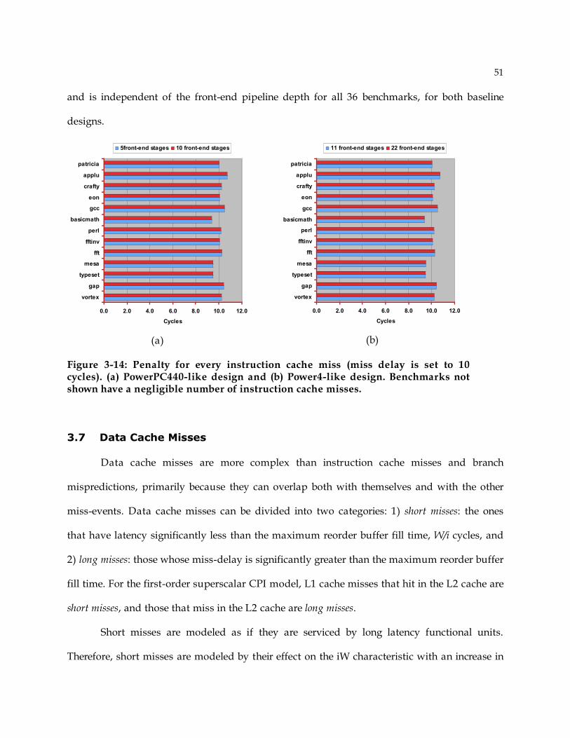
51

and is independent of the front-end pipeline depth for all 36 benchmarks, for both baseline

designs.

(a) (b)

Figure 3-14: Penalty for every instruction cache miss (miss delay is set to 10 cycles). (a) PowerPC440-like design and (b) Power4-like design. Benchmarks not shown have a negligible number of instruction cache misses.

3.7 Data Cache Misses

Data cache misses are more complex than instruction cache misses and branch

mispredictions, primarily because they can overlap both with themselves and with the other

miss-events. Data cache misses can be divided into two categories: 1) short misses: the ones

that have latency significantly less than the maximum reorder buffer fill time, W/i cycles, and

2) long misses: those whose miss-delay is significantly greater than the maximum reorder buffer

fill time. For the first-order superscalar CPI model, L1 cache misses that hit in the L2 cache are

short misses, and those that miss in the L2 cache are long misses.

Short misses are modeled as if they are serviced by long latency functional units.

Therefore, short misses are modeled by their effect on the iW characteristic with an increase in

0.0 2.0 4.0 6.0 8.0 10.0 12.0

vortex

gap

typeset

mesa

fft

fftinv

perl

basicmath

gcc

eon

crafty

applu

patricia

Cycles

5front-end stages 10 front-end stages

0.0 2.0 4.0 6.0 8.0 10.0 12.0

vortex

gap

typeset

mesa

fft

fftinv

perl

basicmath

gcc

eon

crafty

applu

patricia

Cycles

11 front-end stages 22 front-end stages

52

the length of the dependence chains by affecting the average function unit latency (see Section

3.4). This leaves long misses for additional modeling.

To model long data cache miss penalty, consider the transient for an isolated long data

cache miss given in Figure 3-15. Initially, the processor is issuing at the steady-state IPC, and a

long data cache miss occurs. The issuing of independent instructions continues, and the re-

order buffer eventually fills. At that point, dispatch will stall, and after all instructions

independent of the load have issued, issue will stall.

After miss delay lmm cycles from the time the load miss is detected, the data returns

from the memory, the missed load commits, and the independent instructions that have

finished execution also commit in program-order. As these instructions commit, reorder buffer

entries become free to accept new instructions. Then, dispatch resumes, and instruction issue

ramps up following the points on iW characteristic.

Figure 3-15: Transient of an isolated data cache miss.

The formula for the cycle penalty of an isolated data cache miss, as just described, is in

equation 3-12, below. The new parameter crf is the number of cycles it takes to fill the re-order

buffer after the missed load is issued.

cdl2 = lmm – crf – cdr + cru (3-12)

53

Just like the instruction cache miss case, cdr and cru offset each other. The phenomenon leading

to this result, however, is different. In the long data cache miss case cdr portion of the miss

delay is overlapped (and therefore hidden) while the processor issues all the independent

instructions it has available. After the load miss data is returned from memory, the processor

takes cru cycles to resume issuing at the steady-state level. Therefore, cdr reduces the effective

miss penalty, while cru increases it.

Because the cdr and cru offset each other, cdl2 is approximately (lmm – crf) cycles. If the

load instruction is the oldest (or nearly so) at the time it issues, then the reorder buffer will

already be full (or nearly so), so crf is approximately zero, and cdl2 will be approximately lmm

cycles. At the other extreme, if the load that misses happens to be the youngest instruction in

the reorder buffer at the time it issues, then it will take approximately W/i cycles to fill the

reorder buffer behind the missed load, where i is provided by equation 3-6. So, the cdl2 will be

approximately [lmm - (W/i)] cycles. For a first-order estimate of cdl2, the mid-point of the two

extremes is used, and cdl2 is simply modeled as [lmm - [(W/i)/2]] cycles.

The mid-point approximation is verified with cycle-accurate simulation experiments. In

the simulation experiment, load misses were isolated from each other; that is, load misses did

not overlap. To artificially isolate load misses, after a naturally occurring load miss, until this

miss came back other misses were converted to hits. Then the next naturally occurring miss

was treated as an actual miss and the load misses that would have occurred before this miss

returned were converted into hits. This process continued up until 100 million dynamic

program instructions were committed. At the time each isolated load miss issued, the number

of instructions ahead of the load instruction in the reorder buffer was recorded.

Simulation experiment results are summarized in Table 3-3 for the two baseline

designs. For each baseline four data points are presented. The Highest column has the

54

benchmark with the highest number of unissued instructions ahead of its load misses in the

ROB. That is, the number of unissued instructions ahead of a load miss at the time the load

issues. The Typical column has the benchmark that represents typical behavior for the 36

benchmarks examined. The Lowest column has the benchmark with the lowest number of

instructions ahead of its load misses. The last column labeled Average has the number of

instructions ahead of a missed load averaged over all 36 benchmarks.

Loads that miss in the L2 cache are issued from the middle of the reorder buffer

(Average column). In both baseline designs, the extreme and typical cases are the same

benchmarks. This suggests that the position from which the load miss is issued is independent

of the microarchitecture and a stronger function of the program’s load dependence

characteristics. Considered over all 36 benchmarks mid-point approximation is reasonable for

estimating crf in a computationally simple way.

Table 3-3: The number of instructions ahead of a load miss when it issues averaged over all load misses in the program, for the Power4-like configuration.

Highest Typical Lowest Average

PowerPC440-like 52 (ghostscript) 34 (bzip2) 8 (ammp) 28

Power4-like 245 (ghostscript) 130 (bzip2) 7 (ammp) 124

Load misses overlap with each other when two or more load misses are issued close

enough to each other so that the later miss(es) are issued before the data for the first miss

returns from memory. This happens when more than one data independent data cache miss

are within W instructions of each other. To model data cache overlaps first the base case of

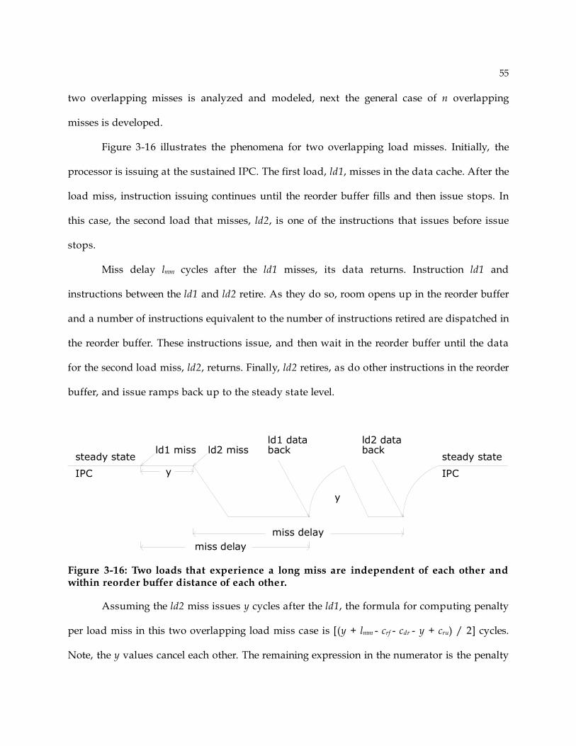
55

two overlapping misses is analyzed and modeled, next the general case of n overlapping

misses is developed.

Figure 3-16 illustrates the phenomena for two overlapping load misses. Initially, the

processor is issuing at the sustained IPC. The first load, ld1, misses in the data cache. After the

load miss, instruction issuing continues until the reorder buffer fills and then issue stops. In

this case, the second load that misses, ld2, is one of the instructions that issues before issue

stops.

Miss delay lmm cycles after the ld1 misses, its data returns. Instruction ld1 and

instructions between the ld1 and ld2 retire. As they do so, room opens up in the reorder buffer

and a number of instructions equivalent to the number of instructions retired are dispatched in

the reorder buffer. These instructions issue, and then wait in the reorder buffer until the data

for the second load miss, ld2, returns. Finally, ld2 retires, as do other instructions in the reorder

buffer, and issue ramps back up to the steady state level.

y

ld1 misssteady state

IPC

ld2 miss

miss delay

miss delay

backld2 data

steady state

IPC

backld1 data

y

Figure 3-16: Two loads that experience a long miss are independent of each other and within reorder buffer distance of each other.

Assuming the ld2 miss issues y cycles after the ld1, the formula for computing penalty

per load miss in this two overlapping load miss case is [(y + lmm - crf - cdr - y + cru) / 2] cycles.

Note, the y values cancel each other. The remaining expression in the numerator is the penalty

56

for an isolated long data-cache miss from equation 3-12. The combined penalty is then the

same as the penalty for an isolated miss. More importantly, the combined penalty is

independent of the distance between the two loads that miss; the only thing that matters is that

the two load misses are data independent of each other and that they occur within W

instructions of each other.

Based on the insight provided by the base case of two overlapping misses, it can be

shown that the miss penalty for n overlapping data-cache misses will be, on average, (lmm/n)

cycles for every miss, and the total penalty is still the same as for an isolated miss. In general,

if there are Nldm long data cache misses and fldm(z) is the probability that misses will occur in

groups of z, the cycle penalty for every miss, on average, is given by equation 3-13, below.

( )

=

! "= # $ %

& '(1

ldmNldm

dc mm

i

f zc c

z (3-13)

The distribution function fldm(z) is collected as a by-product of the instruction trace analysis,

described earlier in Section 3.2. During the trace analysis, the loads that miss in the subject L2

cache are marked. Next, dynamic instruction sequences in lengths equal to the reorder buffer

sizes, available in the component database, are examined. For each set of dynamic

instructions, the number of load misses is recorded. This yields the distribution fldm(z) of

overlapping load misses for every reorder buffer size.

Comparison of the penalty computed using the method just described and the penalty

generated with cycle-accurate simulation is in Figure 3-17. Figure 3-17(a) plots the results for

the PowerPC440-like baseline and Figure 3-17(b) plots the results for the Power4-like baseline.

For both baseline designs, simulation results support equation 3-13. The model penalty tracks

the simulated penalty and is reasonably close to it. The penalty difference is 3.3 percent overall

for both baseline designs.

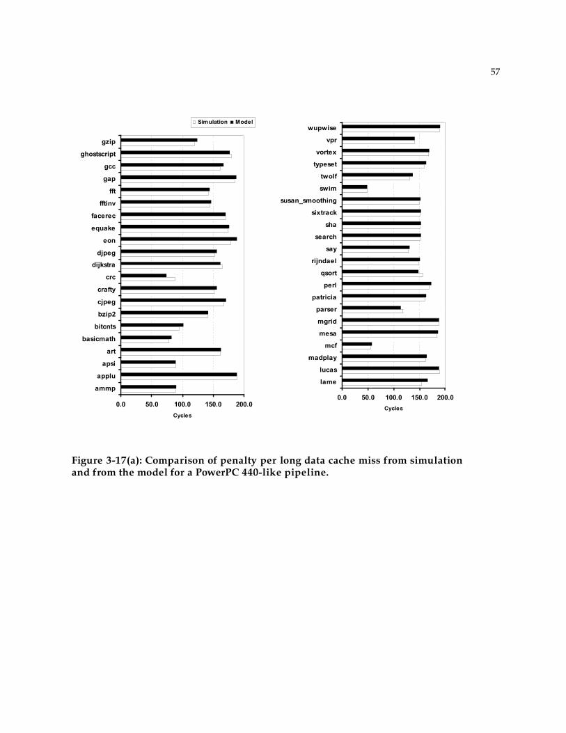
57

Figure 3-17(a): Comparison of penalty per long data cache miss from simulation and from the model for a PowerPC 440-like pipeline.

0.0 50.0 100.0 150.0 200.0

ammp

applu

apsi

art

basicmath

bitcnts

bzip2

cjpeg

crafty

crc

dijkstra

djpeg

eon

equake

facerec

fftinv

fft

gap

gcc

ghostscript

gzip

Cycles

Simulation Model

0.0 50.0 100.0 150.0 200.0

lame

lucas

madplay

mcf

mesa

mgrid

parser

patricia

perl

qsort

rijndael

say

search

sha

sixtrack

susan_smoothing

swim

twolf

typeset

vortex

vpr

wupwise

Cycles

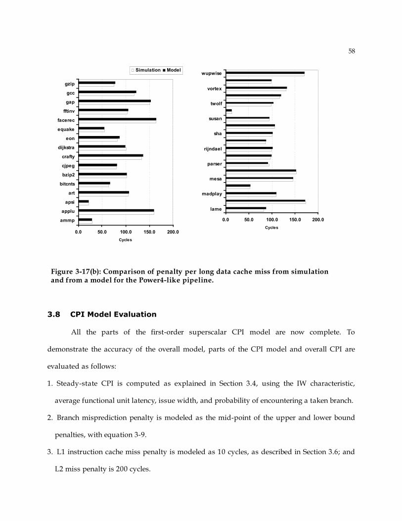
58

Figure 3-17(b): Comparison of penalty per long data cache miss from simulation and from a model for the Power4-like pipeline.

3.8 CPI Model Evaluation

All the parts of the first-order superscalar CPI model are now complete. To

demonstrate the accuracy of the overall model, parts of the CPI model and overall CPI are

evaluated as follows:

1. Steady-state CPI is computed as explained in Section 3.4, using the IW characteristic,

average functional unit latency, issue width, and probability of encountering a taken branch.

2. Branch misprediction penalty is modeled as the mid-point of the upper and lower bound

penalties, with equation 3-9.

3. L1 instruction cache miss penalty is modeled as 10 cycles, as described in Section 3.6; and

L2 miss penalty is 200 cycles.

0.0 50.0 100.0 150.0 200.0

ammp

applu

apsi

art

bitcnts

bzip2

cjpeg

crafty

dijkstra

eon

equake

facerec

fftinv

gap

gcc

gzip

Cycles

Simulation Model

0.0 50.0 100.0 150.0 200.0

lame

madplay

mesa

parser

rijndael

sha

susan

twolf

vortex

wupwise

Cycles

59

4. Long data cache miss penalty is calculated with equation 3-12 taking ldc as 200 cycles.

5. Trace-driven simulations are used to arrive at the numbers of branch mispredictions,

instruction cache misses, data cache misses, and distributions of the bursts of long data

cache misses that occur within W instructions of a previous long data cache miss.

6. Steady-state CPI and additional CPI losses due to each type of miss-event are computed.

Then the CPIs are added (see equation 3-1) to calculate the total CPI.

3.8.1 Evaluation Metrics

The following two metrics are used to compare the analytical CPI model to the cycle-

accurate simulation model: correlation coefficient, and histogram of differences. Collectively these

two metrics support a thorough evaluation of the analytical energy activity model.

The correlation coefficient is a number between zero and one that tells how closely the

analytical model and simulation track each other. A correlation coefficient of one means that

the analytical model and cycle-accurate simulation agree on all points in the design space. A

correlation coefficient of zero means that the analytical model does not model the simulated

phenomenon.

The Histogram of differences between the analytical model and simulation estimates is

useful because if the histogram is Normally distributed, the phenomena not covered by the

first-order model lead to random effects and therefore the first-order model is a sound model

from a statistical perspective [49]. More importantly, Normally distributed differences means

that the first-order model provides a least-mean square error fit, and can therefore be used for

making a relative comparison of two or more superscalar designs for choosing the Pareto-

optimal designs.

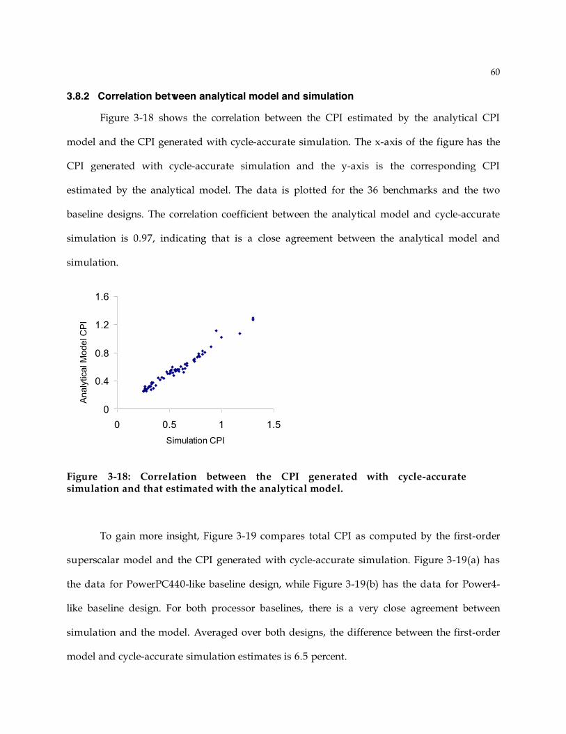
60

3.8.2 Correlation between analytical model and simulation

Figure 3-18 shows the correlation between the CPI estimated by the analytical CPI

model and the CPI generated with cycle-accurate simulation. The x-axis of the figure has the

CPI generated with cycle-accurate simulation and the y-axis is the corresponding CPI

estimated by the analytical model. The data is plotted for the 36 benchmarks and the two

baseline designs. The correlation coefficient between the analytical model and cycle-accurate

simulation is 0.97, indicating that is a close agreement between the analytical model and

simulation.

0

0.4

0.8

1.2

1.6

0 0.5 1 1.5

Simulation CPI

Analy

tical M

odel C

PI

Figure 3-18: Correlation between the CPI generated with cycle-accurate simulation and that estimated with the analytical model.

To gain more insight, Figure 3-19 compares total CPI as computed by the first-order

superscalar model and the CPI generated with cycle-accurate simulation. Figure 3-19(a) has

the data for PowerPC440-like baseline design, while Figure 3-19(b) has the data for Power4-

like baseline design. For both processor baselines, there is a very close agreement between

simulation and the model. Averaged over both designs, the difference between the first-order

model and cycle-accurate simulation estimates is 6.5 percent.

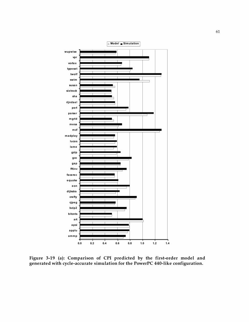
61

0.0 0.2 0.4 0.6 0.8 1.0 1.2 1.4

ammp

applu

apsi

art

bitcnts

bzip2

cjpeg

crafty

dijkstra

eon

equake

facerec

fftinv

gap

gcc

gzip

lame

lucas

madplay

mcf

mesa

mgrid

parser

perl

rijndael

sha

sixtrack

susan

swim

twolf

typeset

vortex

vpr

wupwise

Model Simulation

Figure 3-19 (a): Comparison of CPI predicted by the first-order model and generated with cycle-accurate simulation for the PowerPC 440-like configuration.

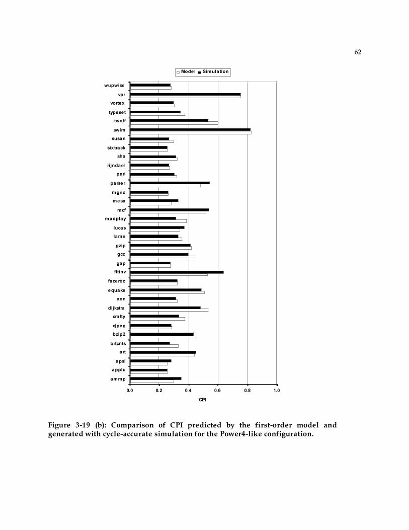
62

0.0 0.2 0.4 0.6 0.8 1.0

ammp

applu

apsi

art

bitcnts

bzip2

cjpeg

crafty

dijkstra

eon

equake

facerec

fftinv

gap

gcc

gzip

lame

lucas

madplay

mcf

mesa

mgrid

parser

perl

rijndael

sha

sixtrack

susan

swim

twolf

typeset

vortex

vpr

wupwise

CPI

Model Simulation

Figure 3-19 (b): Comparison of CPI predicted by the first-order model and generated with cycle-accurate simulation for the Power4-like configuration.

63

Overall, the CPI difference is 6.5 percent on average. In the PowerPC440-like design

case, absolute CPI difference averaged over all 36 benchmarks is 5 percent. For the case of

Power4-like design, absolute CPI difference averaged over all benchmarks is 8 percent.

Benchmark madplay is an outlier with the highest CPI difference of 23 percent, with the

Power4-like design.

The CPI difference for madplay is as high as it is because of the modeling of branch

misprediction penalty. Figure 3-20 compares various CPI components estimated by the

analytical model and generated through simulation for madplay. A large fraction of the total

CPI is because of branch mispredictions. Further, the greatest discrepancy is because of branch

misprediction CPI.

The reason for the discrepancy in branch misprediction CPI for madplay is that the

mispredictions are clustered together in simulation, resulting in the penalty for every

misprediction equal to the lower bound (see Section 3.3 of this chapter). Mid-point

approximation however does not model clustering of mispredictions for computational

simplicity and simply computes the mid-point of two extremes. This results in a higher

penalty for madplay. A more refined model called Interval Analysis[48] that models clustered

mispredictions has been developed and can be used to reduce overall CPI difference if needed.

64

madplay CPI breakdown comparison

0 0.05 0.1 0.15 0.2 0.25 0.3

Ideal CPI

Icache miss CPI

Long Dcache

miss CPI

Branch

Misprediction

CPI

CPI

Model

Simulation

Figure 3-20: CPI breakdown comparison for madplay shows that the high CPI difference of 23 percent is due to branch mispredictions.

To gain further insight into the difference between the analytical model and cycle-

accurate simulation, Figure 3-21 plots the distribution of CPI differences for both baseline

designs. The histogram is a Normal distribution with a Shapiro-Wilks goodness-of-fit

value[50] of 0.97 out of a maximum possible value of 1; when the histogram is a perfect

Normal distribution the value is 1. Mathematically, this result indicates that the first-order

model provides a least-mean square error fit – statistically the best possible fit -- for the cycle-

accurate simulation CPI estimates [50]. This characteristic of the differences imply that the

phenomena the first-order analytical model abstracts out is random, and therefore the model

will always track the cycle-accurate simulation estimates [50]. Consequently, the first-order

analytical CPI model is sufficient for modeling out-of-order superscalar processors and

gauging relative CPI trade-offs between two or more designs.

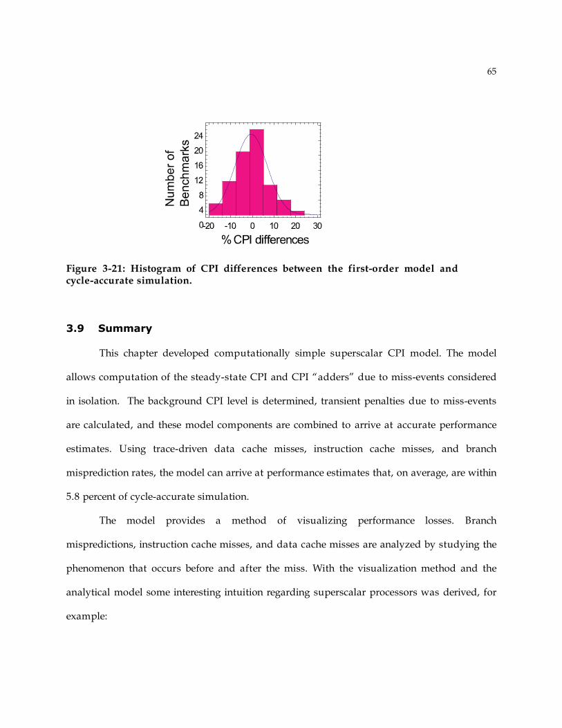
65

Figure 3-21: Histogram of CPI differences between the first-order model and cycle-accurate simulation.

3.9 Summary

This chapter developed computationally simple superscalar CPI model. The model

allows computation of the steady-state CPI and CPI “adders” due to miss-events considered

in isolation. The background CPI level is determined, transient penalties due to miss-events

are calculated, and these model components are combined to arrive at accurate performance

estimates. Using trace-driven data cache misses, instruction cache misses, and branch

misprediction rates, the model can arrive at performance estimates that, on average, are within

5.8 percent of cycle-accurate simulation.

The model provides a method of visualizing performance losses. Branch

mispredictions, instruction cache misses, and data cache misses are analyzed by studying the

phenomenon that occurs before and after the miss. With the visualization method and the

analytical model some interesting intuition regarding superscalar processors was derived, for

example:

66

1. The branch misprediction penalty is can be significantly greater then the front-end pipeline

depth.

2. Instruction cache penalty is independent of the front-end pipeline; it depends largely on the

miss delay.

3. The data cache penalty for an isolated long miss is essentially the miss delay. For multiple

misses that occur within a number of instructions equal to the reorder buffer size, the

combined miss penalty is the same as an isolated miss.

Compared to cycle-accurate simulations the model provides accurate CPI estimates.

The model tracks cycles per instruction values generated with cycle accurate simulation. For

the PowerPC440-like configuration the differences are within 10 percent and for the Power4-

like configuration the differences are within 12 percent.

From a statistical perspective this model is sufficient for CPI estimation. The

correlation coefficient between the analytical model CPI and cycle-accurate simulation CPI is

0.97, indicating a strong correlation between the model and cycle-accurate simulation. The CPI

differences between the cycle-accurate simulation and the model follow a Normal distribution

for the 36 benchmarks indicating that the analytical model is good for estimating the CPI.

The fundamental principles developed for this CPI model are used for the energy

activity model described in the next chapter. In chapter 5, the search method leverages the

computational simplicity and the insights from the CPI model to find Pareto-optimal

configurations in terms of CPI, energy, and silicon area for the target application program.

67

Chapter 4: Energy Activity Model

Determining energy consumption of a target program running on a specific processor

configuration is another important aspect of a design optimization method. Energy

consumption can be expressed as

( )!

"# Energy activity of type Energy consumed for activity of type EAi S

i i ,

where SEA is the set of all energy activities. Hence, determining both the types of energy

activities and the energy consumed for a particular type of activity are important parts of a

design optimization method.

Energy activity of a particular type is a function of the program and the

microarchitecture. Energy consumed for a particular type of energy activity is determined by

the implementation technology, circuit design, logic-gate design, and the layout. Because this

dissertation provides a method of optimizing the microarchitecture, this chapter focuses on

energy activities by describing a new method of quantifying energy activities and providing

analytical models to quickly compute energy activities.

Energy activity multipliers for a specific component can be obtained in number of ways

[51-53]. One option is to generate energy multipliers by simulating each component with

HSPICE [54]. Another option is to use first-order circuit-level methods such as state-transition

diagrams [55-57]. A comprehensive survey of logic-gate level and circuit level tools for

computing energy is provided by Najm in [58]. In this dissertation, the energy multipliers are

computed with a library of energy activity multipliers provided as part of Wattch [59]. Energy

68

is calculated with a product of energy activities and their respective multipliers, as given in the

above equation.

4.1 Quantifying Energy Activity

The method of quantifying energy activity is based on the inherent properties of digital

logic structures that constitute microprocessors. Fundamentally, microprocessors must be able

to do the following three things: 1) perform computations, for example addition of two

numbers; 2) store and retrieve state, for example temporarily storing instructions in the L1

cache; and 3) synchronize information processing, for example ordering instructions in between

two pipeline stages.

The ability to compute requires combinational logic. Storing and retrieving state requires

structures that provide storage without taking up a lot of area, referred to in this chapter as

memory cells. The ability to synchronize requires flip-flops. Combinational logic, memory cells, and

flip-flops are then building blocks of all microprocessor components. Energy activities of any

component can be derived from the operational characteristics of its building block(s).

4.1.1 Combinational logic

An example of a combinational logic component is the integer arithmetic and logic unit

(ALU). In a given clock cycle, integer ALU is either used as part of the ongoing computation or

it is not. The same holds true for various other combinational logic components. Consequently,

a combinational logic component is defined to be Active if its results are used by the ongoing

computation during a given cycle, and it is defined to be Idle if its results are not used during

a clock cycle.

69

4.1.2 Memory cells

Memory cells are used in components that have high density storage requirements, for

example caches, physical register files, and branch predictors. A one-bit memory cell is

illustrated in Figure 4-1. The memory cell has a cross-coupled inverter to store a datum. The b

and b_n inputs (b_n is the logical complement of b) are used for reading and writing

information into the cross-coupled inverter. The access signal determines when information is

read and written in the cross-coupled inverters. When access is high the nMOS transistors

provide a path to the cross-coupled inverter for reading and writing. When access is low the

nMOS transistors the information in the cross-coupled inverter cannot be read or written.

Figure 4-1: High-level diagram of a memory cell.

In a clock cycle, the access signal of the memory cell can be either high or low. As a

result two activities are used to model memory cells. A memory element is Active when the

access signal is high; it is Idle when the access signal is low. Based on this observation, a

component constructed from memory cells, for example L1 instruction cache, is Active when

accessed and Idle when not accessed.

4.1.3 Flip-flops

Flip-flops propagate the input to the output only at the rising or falling edge of the clock

signal and are therefore used for synchronization and for maintaining order at the end of every

clock cycle, for example in pipeline stages and queues. A one-bit flip-flop used in a pipeline

b

access

b_n

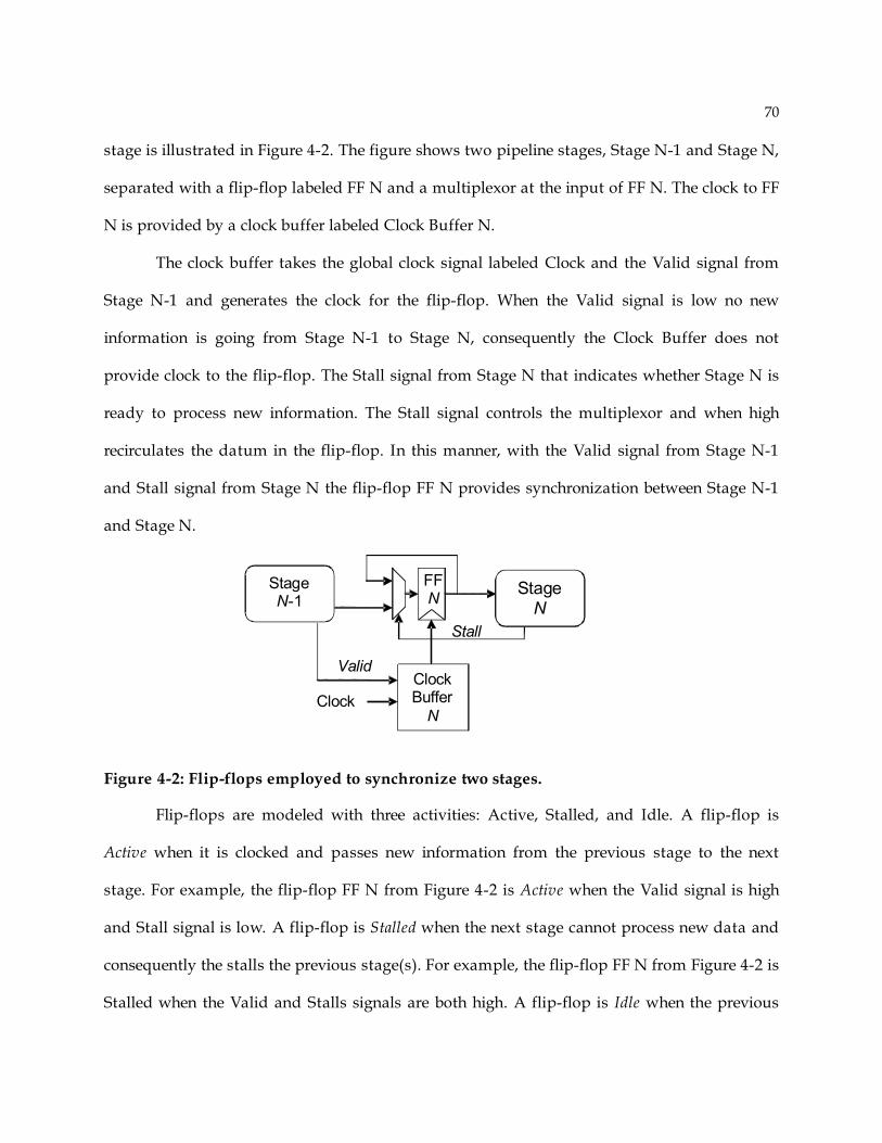
70

stage is illustrated in Figure 4-2. The figure shows two pipeline stages, Stage N-1 and Stage N,

separated with a flip-flop labeled FF N and a multiplexor at the input of FF N. The clock to FF

N is provided by a clock buffer labeled Clock Buffer N.

The clock buffer takes the global clock signal labeled Clock and the Valid signal from

Stage N-1 and generates the clock for the flip-flop. When the Valid signal is low no new

information is going from Stage N-1 to Stage N, consequently the Clock Buffer does not

provide clock to the flip-flop. The Stall signal from Stage N that indicates whether Stage N is

ready to process new information. The Stall signal controls the multiplexor and when high

recirculates the datum in the flip-flop. In this manner, with the Valid signal from Stage N-1

and Stall signal from Stage N the flip-flop FF N provides synchronization between Stage N-1

and Stage N.

Figure 4-2: Flip-flops employed to synchronize two stages.

Flip-flops are modeled with three activities: Active, Stalled, and Idle. A flip-flop is

Active when it is clocked and passes new information from the previous stage to the next

stage. For example, the flip-flop FF N from Figure 4-2 is Active when the Valid signal is high

and Stall signal is low. A flip-flop is Stalled when the next stage cannot process new data and

consequently the stalls the previous stage(s). For example, the flip-flop FF N from Figure 4-2 is

Stalled when the Valid and Stalls signals are both high. A flip-flop is Idle when the previous

Stage N-1

Stage N

Clock Buffer

N

FF N

Stall

Clock

Valid

71

stage does not have valid information. For example, if Stage N-1 does not have valid

information the Valid signal will be low and consequently, irrespective of the Stall signal, the

flip-flop is not clocked.

This overall method of quantifying energy at the microarchitecture-level with three

activities is henceforth referred to as the ASI method. Table 4.1 summarizes the three activities

and what each activity means for each of the three component building blocks. In general,

Active and Idle activities are applicable to all building blocks and therefore all components.

Stalled activity is applicable only to flip-flops and components built from flip-flops.

Table 4-1: Summary of component building blocks and their energy activities.

Building Block Active Stall Idle

Combinational Logic Accessed N/A Not accessed

Memory element Accessed N/A Not accessed

Flip-flop Accepting new data Holding contents Contents not

valid

4.1.4 Modeling Miss-speculated Activities

The Active, Stalled, and Idle activities are further decomposed into two groups to

account for energy activity consumed because of branch mispredictions. One group is for

instructions that eventually commit, referred to as Used. The other group is for instructions on

a mispredicted path called Flushed. For example, the activity for instructions that are issued

but later discarded is called Active Flushed.

72

4.1.5 Insight provided by the ASI method

The ASI method provides insight into the ways that energy is consumed. For example,

a designer can evaluate the amount of energy activity that can be saved by reducing the events

that contribute to Stalled and Idle activities. The ASI breakdown can also guide development

of logic-level and circuit-level techniques for minimizing Stalled and Idle activity multipliers.

Because each activity is decomposed into Used and Flushed parts, energy consumption due to

branch mispredictions is modeled. This breakdown can help assess the cost of mispeculation

from the energy consumption point-of-view.

Combining the above two observations, the ASI method reveals that Active-Used is the

absolutely necessary energy activity for executing a program. Other activities are not essential

and should be minimized; even Stalled activity on the correct-path is not considered to be

essential activity. These observations are employed in work by Karkhanis et al. [38] to reduce

energy consumption because of instruction stalls and mispeculation.

4.1.6 ASI method versus Utilization method

The ASI method is more comprehensive than the conventional utilization method[60].

The utilization method reports a number between zero and one for the fraction of the clock

cycles a component has valid information. ASI method provides more insight than the

utilization method by separating utilization into Active and Stalled components.

Consider the front-end pipeline flip-flop with valid-bit clock gating in Figure 4-2 for

comparing the two methods. When the flip-flop is Active it has a free-running clock and its

internal nodes are switching because new data is being captured. Therefore, energy is

consumed for switching of the clock signal, switching of the internal nodes of the flip-flop, and

leakage. When Stalled the flip-flop has a free-running clock, but the internal nodes do not

73

switch. Energy is consumed because of clock switching and leakage. When the flip-flop is Idle,

neither the clock at the input of the flip-flop switches nor do the internal nodes of the flip-flop

– only static leakage energy is consumed in the Idle state. In this example Active consumes

more energy than Stalled, and Stalled consumes more energy than Idle.

Suppose valid data is moving from stage N to stage N-1 every cycle. The utilization

method will report a one, because the flip-flop has valid information every cycle. The ASI

method will classify this phenomenon as Active, with the magnitude equal to the number of

cycles pipeline stage N is processing new information.

Now suppose stage N stalls and the flip-flop holds the information for the duration of

the stall. The utilization method will report a one, because the flip-flop has valid information.

The ASI method, on the other hand, will classify this phenomenon as Stalled activity, with a

magnitude of the number of cycles equal to the duration of the stall.

Stalls such as the one in this example occur frequently in the front-end pipeline of

microprocessors. Energy consumed for such stalls can be considered wasted because

instructions are fetched earlier than necessary. The utilization method is unable to differentiate

the situation where information is being processed from the situation where processing is

stalled. Because of this limitation the utilization method arrives at an imprecise energy

estimate for components that consume different amounts of energy when processing

information than when holding information. Consequently, the utilization method does not

provide the insight that energy can be reduced by avoiding stalls.

The ASI method distinguishes useful Active activity and the useless Stalled activity.

Because of this the ASI method can more precisely model valid-bit clock gating and other

methods such as power-gating [61] that leverage the different operational characteristics of the

component building blocks for energy reduction. Equally important, is the insight regarding the

74

Stalled and Idle activities that the ASI method provides. With the ASI method it is clear that

Stalled and Idle activities are inessential activities.

4.2 ASI Method Validation

The ASI method is validated by comparing its estimates to four industrial

implementations -- two embedded processors and two desktop/server class processors. The

embedded processors are the MIPS R10000 and PowerPC 440, and the server class reference

designs are the IBM Power4 and Alpha 21264. The power dissipation data for the reference

designs is taken from published conference and journal papers and from product datasheets.

For the validation the ASI method is implemented in a cycle-accurate simulator, by

embedding counters for measuring various energy activities in the simulator. Energy activity

multipliers are taken from power.h file of Wattch. Energy consumed is then computed as the

product of the energy activities and the respective activity multipliers. To compute the power

dissipation, the energy estimates are divided by the published clock-rate of the specific

reference processor design. Then, an arithmetic mean of the power dissipation is computed

over all 35 benchmarks. This result is compared to the published power dissipation data of

industrial processor implementations. Figure 4-3 has the results. Overall, the ASI method

coupled with energy multipliers from Wattch tracks the actual processor implementation

estimates.

The differences between the cycle-accurate simulator and the actual implementation are

due to random logic that is not modeled in the cycle-accurate simulator; for example

interconnects and test circuitry. Another source of error is the custom circuitry used for Power4

and Alpha 21264 processors [44, 62]. Power4 and Alpha 21264 have the two highest

differences because of the custom circuit design employed in designing these microprocessors.

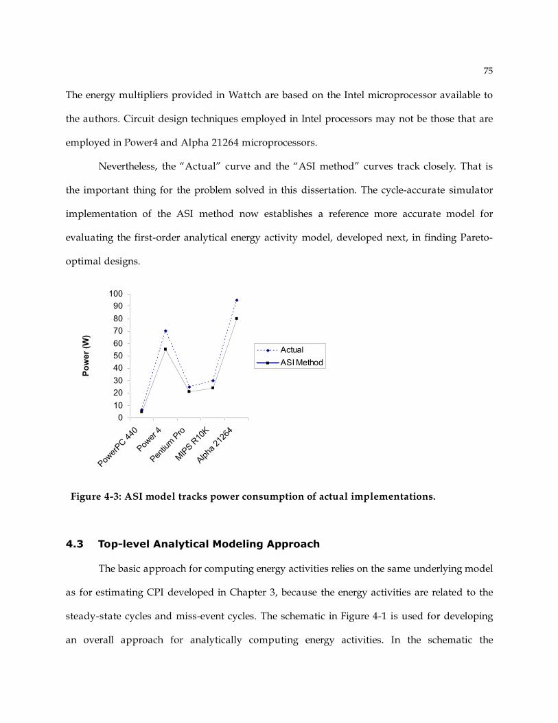
75

The energy multipliers provided in Wattch are based on the Intel microprocessor available to

the authors. Circuit design techniques employed in Intel processors may not be those that are

employed in Power4 and Alpha 21264 microprocessors.

Nevertheless, the “Actual” curve and the “ASI method” curves track closely. That is

the important thing for the problem solved in this dissertation. The cycle-accurate simulator

implementation of the ASI method now establishes a reference more accurate model for

evaluating the first-order analytical energy activity model, developed next, in finding Pareto-

optimal designs.

0

10

20

30

40

50

60

70

80

90

100

Pow

erPC 4

40

Pow

er 4

Pentiu

m P

ro

MIP

S R10

K

Alpha

212

64

Po

wer

(W)

Actual

ASI Method

Figure 4-3: ASI model tracks power consumption of actual implementations.

4.3 Top-level Analytical Modeling Approach

The basic approach for computing energy activities relies on the same underlying model

as for estimating CPI developed in Chapter 3, because the energy activities are related to the

steady-state cycles and miss-event cycles. The schematic in Figure 4-1 is used for developing

an overall approach for analytically computing energy activities. In the schematic the

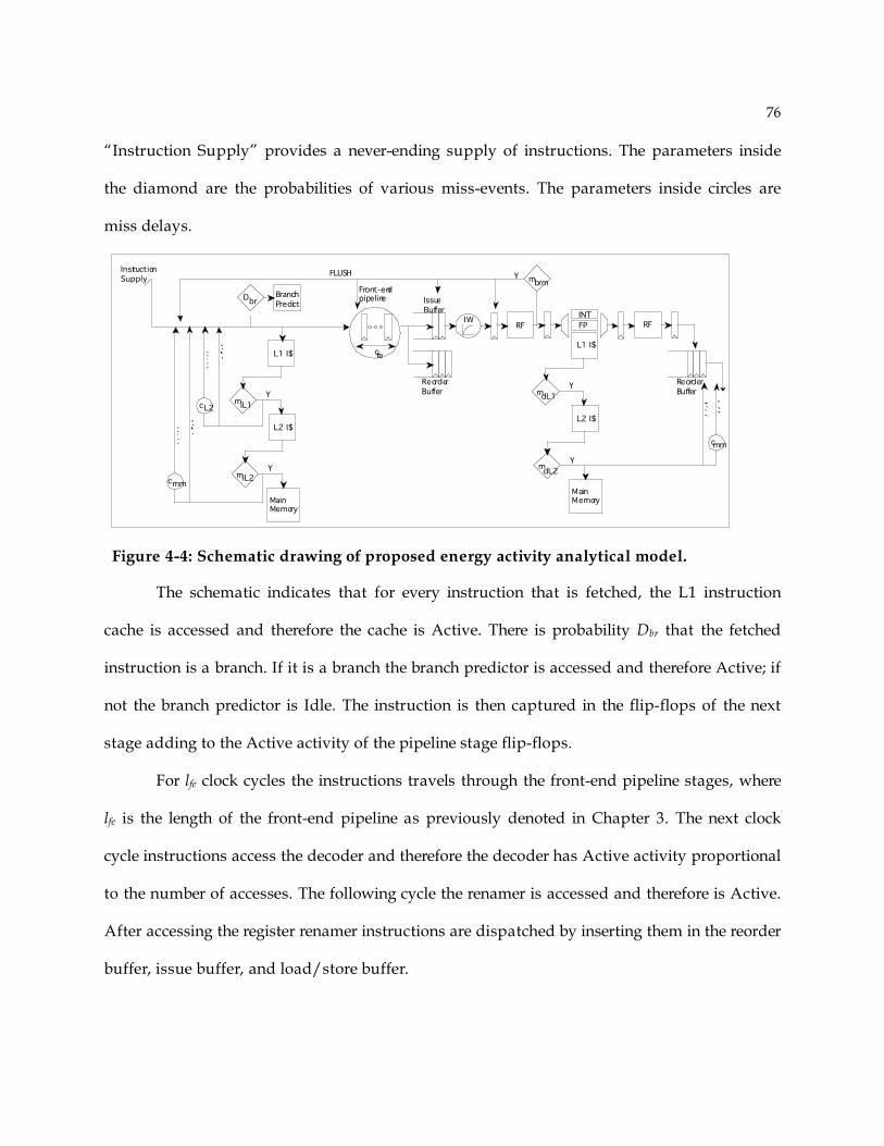
76

“Instruction Supply” provides a never-ending supply of instructions. The parameters inside

the diamond are the probabilities of various miss-events. The parameters inside circles are

miss delays.

L1 I$

L2 I$

MainMemory

mY

mY

c L2

c mmiL2

iL1

cfe

IssueBuffer

ReorderBuffer

IWRF

INT

FP

L1 I$

L2 I$

mY

dL1

mY

dL2

Front-endpipeline

MainMemory

RF

ReorderBuffer

cmm

mbrmY

InstructionSupply

FLUSH

DbrBranchPredict

Figure 4-4: Schematic drawing of proposed energy activity analytical model.

The schematic indicates that for every instruction that is fetched, the L1 instruction

cache is accessed and therefore the cache is Active. There is probability Dbr that the fetched

instruction is a branch. If it is a branch the branch predictor is accessed and therefore Active; if

not the branch predictor is Idle. The instruction is then captured in the flip-flops of the next

stage adding to the Active activity of the pipeline stage flip-flops.

For lfe clock cycles the instructions travels through the front-end pipeline stages, where

lfe is the length of the front-end pipeline as previously denoted in Chapter 3. The next clock

cycle instructions access the decoder and therefore the decoder has Active activity proportional

to the number of accesses. The following cycle the renamer is accessed and therefore is Active.

After accessing the register renamer instructions are dispatched by inserting them in the reorder

buffer, issue buffer, and load/store buffer.

77

Instructions are issued from the issue buffer following the IW Characteristic; unissued

instructions wait in the issue buffer. The issue buffer therefore experiences Active activity for

issuing instructions and Stalled activity for holding the unissued instructions. If the issued

instructions need to read registers, the physical register file is accessed and therefore is Active.

During the following cycle, instructions are sent to their corresponding function unit for

execution. The function units that are accessed during that clock cycle are Active; the function

units that are not accessed stay Idle.

After execution, instructions that write to a destination register access the physical

register file. Consequently, the physical register file can be Active in that cycle. Finally, when

the instruction retires the register renamer is accessed for returning the physical register and is

therefore Active.

There is a probability mil1 that a fetched instruction results in a L1 instruction cache

miss. When an instruction cache miss occurs, instruction fetch stops for the miss delay cycle.

During this time the instructions that are in the front-end pipeline and the reorder buffer

continues processing. As these instructions move through the pipeline stages, components in

the front-end pipeline become Idle. Components in stages close to the fetch stage become Idle

first, and in subsequent cycles components in stages further away from fetch progressively

become Idle.

The missed instructions are available from the L2 cache after miss delay ll2 cycles, and

then they enter the processor pipeline. The front-end components then become Active for

processing the instructions. The Fetch stage becomes Active first, then on subsequent cycles the

fetched instructions moves from through the pipeline towards the commit stage. As the

instructions move, components in each stage become Active. Effectively, every component is

Idle for ll2 cycles on every instruction cache miss. The same phenomenon occurs with

78

probability mil2 for instructions that miss in the L2 unified cache. For the L2 cache miss case

the components are Idle for L2 cache miss delay lmm cycles.

When a long data cache miss happens with a probability mdl2, the instruction commit

soon stops. Shortly thereafter the reorder buffer fills and dispatch stops. Because instructions

cannot be dispatched, instruction fetch stops; no new instructions are fetched until the missed

data is delivered from memory. During this time instructions are held in the flip-flops between

pipeline stages, in the reorder buffer, issue buffer, and the load store buffer. The entries in these

components that are not occupied are Idle. No combinational logic components are switching

and no memory element components are accessed. Consequently, combination logic and

memory element-based components experience Idle activity, while flip-flop based components

experience Stalled activity.

When a branch misprediction occurs, instruction processing continues as usual. The

difference however is that after the branch misprediction is detected, all miss-speculated

instructions are flushed. After the flush, components are Idle during the time taken for correct-

path instructions to reach the components. The exact Idle activity of the components is a

function of the position of the component in the processor pipeline. Components in the fetch

stage, for example, fetch correct-path instructions immediately after the flush and therefore do

not experience Idle activity. Components in stages away from the fetch stage, for example the

function units, are Idle until correct-path instructions issue.

On the mispredicted path, the energy activities will be the same as they under normal

conditions. The only difference is that these activities are non-essential, and the amount of the

non-essential activity depends on the number of miss-speculated instructions a component has

to process. Furthermore, components in pipeline stages away from the fetch stage experience

more Idle activity due to mispredictions than the components in the fetch stage.

79

Based on the schematic in Figure 4-3, the following observations can be made:

1. Under ideal conditions components in the processor core, L1 caches, and L2 cache can be

Active, Stalled, or Idle; main memory is Idle.

2. Because of instruction cache misses, components within the processor core become Idle

(Active and Stall activities are zero); the only component that is Active is higher level cache

or the main memory.

3. Because of long data cache misses, flip-flop based components are Stalled, other

components are Idle; only the main memory is Active.

4. When there is a branch misprediction, instruction processing proceeds just as with normal

conditions; the only difference is that the energy activity is non-essential.

From the above observations, the following two further observations follow:

1. Total Used energy activities of a component are computed by adding energy activities under

ideal conditions and the additional Used energy activities due to cache misses.

2. Flushed energy activities are computed with the same method used to compute Used

activities. The only additional information required is the number of miss-speculated

instructions that each component processes.

The rest of this chapter develops analytical models for computing energy activities of

various components using the two concluding observations listed above. The overall approach

to arriving at energy activities is: 1) compute the Used portion of each type of energy activity,

2) compute the number of miss-speculated cycles a component experiences, and 3) compute

the Flushed portion of energy activity assuming the miss-speculated instructions have the

same program statistics as the correct path instructions.

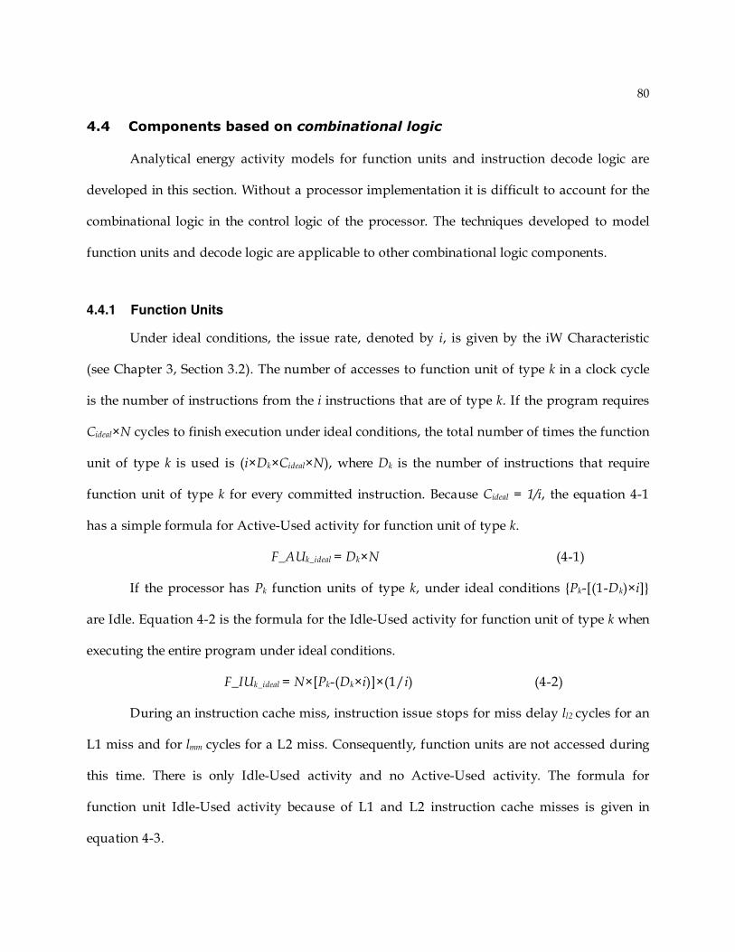
80

4.4 Components based on combinational logic

Analytical energy activity models for function units and instruction decode logic are

developed in this section. Without a processor implementation it is difficult to account for the

combinational logic in the control logic of the processor. The techniques developed to model

function units and decode logic are applicable to other combinational logic components.

4.4.1 Function Units

Under ideal conditions, the issue rate, denoted by i, is given by the iW Characteristic

(see Chapter 3, Section 3.2). The number of accesses to function unit of type k in a clock cycle

is the number of instructions from the i instructions that are of type k. If the program requires

Cideal×N cycles to finish execution under ideal conditions, the total number of times the function

unit of type k is used is (i×Dk×Cideal×N), where Dk is the number of instructions that require

function unit of type k for every committed instruction. Because Cideal = 1/i, the equation 4-1

has a simple formula for Active-Used activity for function unit of type k.

F_AUk_ideal = Dk×N (4-1)

If the processor has Pk function units of type k, under ideal conditions {Pk-[(1-Dk)×i]}

are Idle. Equation 4-2 is the formula for the Idle-Used activity for function unit of type k when

executing the entire program under ideal conditions.

F_IUk_ideal = N×[Pk-(Dk×i)]×(1/i) (4-2)

During an instruction cache miss, instruction issue stops for miss delay ll2 cycles for an

L1 miss and for lmm cycles for a L2 miss. Consequently, function units are not accessed during

this time. There is only Idle-Used activity and no Active-Used activity. The formula for

function unit Idle-Used activity because of L1 and L2 instruction cache misses is given in

equation 4-3.

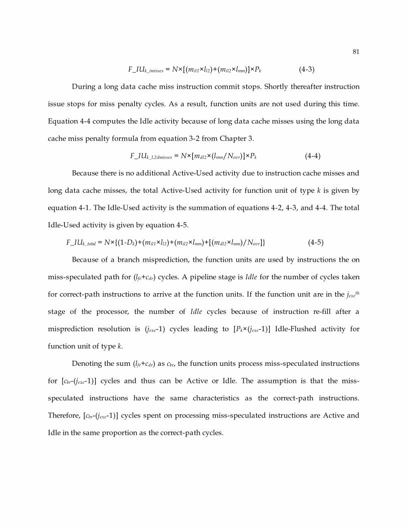
81

F_IUk_imisses = N×[(mil1×ll2)+(mil2×lmm)]×Pk (4-3)

During a long data cache miss instruction commit stops. Shortly thereafter instruction

issue stops for miss penalty cycles. As a result, function units are not used during this time.

Equation 4-4 computes the Idle activity because of long data cache misses using the long data

cache miss penalty formula from equation 3-2 from Chapter 3.

F_IUk_L2dmisses = N×[mdl2×(lmm/Novr)]×Pk (4-4)

Because there is no additional Active-Used activity due to instruction cache misses and

long data cache misses, the total Active-Used activity for function unit of type k is given by

equation 4-1. The Idle-Used activity is the summation of equations 4-2, 4-3, and 4-4. The total

Idle-Used activity is given by equation 4-5.

F_IUk_total = N×{(1-Dk)+(mil1×ll2)+(mil2×lmm)+[(mdl2×lmm)/Novr]} (4-5)

Because of a branch misprediction, the function units are used by instructions the on

miss-speculated path for (lfe+cdr) cycles. A pipeline stage is Idle for the number of cycles taken

for correct-path instructions to arrive at the function units. If the function unit are in the jexeth

stage of the processor, the number of Idle cycles because of instruction re-fill after a

misprediction resolution is (jexe-1) cycles leading to [Pk×(jexe-1)] Idle-Flushed activity for

function unit of type k.

Denoting the sum (lfe+cdr) as cbr, the function units process miss-speculated instructions

for [cbr-(jexe-1)] cycles and thus can be Active or Idle. The assumption is that the miss-

speculated instructions have the same characteristics as the correct-path instructions.

Therefore, [cbr-(jexe-1)] cycles spent on processing miss-speculated instructions are Active and

Idle in the same proportion as the correct-path cycles.

82

The above two phenomena occur on every mispredicted branch, and there are (N×mbr)

mispredicted branches in a program. Equation 4-6, and 4-7, therefore, compute the Active-

Flushed, and Idle-Flushed activities, respectively, for function unit of type k.

F_AFk_total = [cbr-(jexe-1)]×[F_AUk/(F_AUk+F_IUk)]×N×mbr (4-6)

F_IFk_total={[cbr-(jexe-1)]×[F_IUk/(F_AUk+F_IUk)]×N×mbr}

+{(jexe-1)×Pk×N×mbr}

(4-7)

4.4.2 Decode Logic

Under ideal conditions the processor sustains a steady-state instruction throughput of i

every cycle, given by the IW Characteristic (see Chapter 3, Section 3.2). As a result, Active-

Used front-end decoder activity i every cycle. Assuming the peak decoder rate is I, average

Idle-Used decoder activity is (I-i) every cycle. Equations 4-8 and 4-9 give the Active-Used and

Idle-Used decoder activities, respectively, for the entire execution of the program.

DE_AUideal = N (4-8)

DE_IUideal = (I/i-1)×N (4-9)

When there is instruction cache miss, instruction fetch stops for miss penalty lmm cycles.

Consequently, instructions are not decoded, and the decoder is Idle. The formula for decode

logic Idle-Used activity due to L1 and L2 instruction cache misses is given in equation 4-10.

DE_IUimisses = I×N×[(mil1×ll2)+(mil2×lmm)] (4-10)

When there is a long data cache miss, instruction commit stops. Shortly thereafter

instruction issue and fetch stop for miss penalty cycles. As a result, the decoder is not used

during this time. The formula for long data cache miss penalty was derived in equation 3-12 of

Chapter 3. Equation 4-11 computes the Idle activity because of long data cache miss using the

long data cache miss penalty equation.

83

DE_IUL2dmisses = N×[mdl2×(lmm/Novr)]×I (4-11)

Because there is no additional Active-Used activity due to instruction cache misses and

long data cache misses, the total Active-Used activity for the decoder is given by equation 4-8.

The Idle-Used activity is the summation of equations 4-9, 4-10, and 4-11. The total Idle-Used

activity is given by the formula in equation 4-12.

DE_IUtotal = I×N×{(1/i-1)+(mil1×ll2)+(mil2×lmm)+[mdl2×(lmm/Novr)]} (4-12)

When there is a branch misprediction, instructions on the miss-speculated path use the

decode logic for cbr cycles including the Idle cycles after the flush. After the pipeline flush the

decoder is Idle for the number of cycles taken for correct-path instructions to arrive at the

decoder. If the decoder is in the jde th stage of the processor, the number of Idle cycles because

of instruction re-fill after the misprediction is (jde-1) cycles leading to [I×(jde-1)] Idle-Flushed

activity for function unit of type k.

For the remaining [cbr-(jde-1)] miss-speculated cycles the decode logic processes miss-

speculated instructions and therefore can be Active or Idle. The assumption is that the miss-

speculated instructions have the same characteristics as the correct-path instructions.

Therefore, [cbr-(jde-1)] cycles spent on processing miss-speculated instructions are Active and

Idle in the same proportion as the correct-path cycles.

The above two phenomena occur on every mispredicted branch. There are (N×mbr)

mispredicted branches in a program. Equation 4-13, and 4-14, therefore, compute the Active-

Flushed, and Idle-Flushed activities, respectively, for the decoder.

DE_AFtotal = [cbr-(jde-1)]×[DE_AU/(DE_AU+ DE_IU)]×N×mbr (4-13)

DE_IFtotal ={[cbr-(jde-1)]×[ DE_IU/(DE_AU+ DE_IU)]×N×mbr}

+{(jde-1)×I×N×mbr}

(4-14)

84

4.5 Components based on memory cells

All memory element based components are modeled with Active and Idle activities. As

mentioned earlier, a memory element based component is Active when accessed and Idle when

not accessed. This section develops analytical models for the level-1 instruction and data

caches, level-2 unified cache, and branch predictor. The modeling method is applicable to other

memory element based processor components such as translation-lookaside buffers.

4.5.1 L1 instruction cache

Under ideal conditions, the L1 instruction cache is accessed every cycle, and L1

instruction cache Active activity is the number of cycles required to execute the program. This

is given in equation 4-15.

L1I$_AUideal = N×1/i (4-15)

When there is an instruction cache miss, fetching of instructions from the L1 instruction

cache stops. Active-Used activity for the L1 instruction cache is zero; the L1 instruction cache

remains Idle until the instructions from the L2 cache are available. Equation 4-16 is formula

for Idle-Used activity for the L1 instruction cache.

L1I$_IUimisses = (Pil1-i)×N×[(mil1×ll2)+(mil2×lmm)] (4-16)

After a long data cache miss, instruction fetch eventually stops. Consequently, Active

activity for the L1 instruction cache is zero for average load miss delay lmm cycles. The Idle

activity because of a long data cache misses is given by equation 4-17 below.

L1I$_IUL2dmisses = (Pil1-i)×N×mdl2×(lmm/Novr) (4-17)

Total Active-Used energy activity is given by equation 4-15, because the L1 instruction

cache does not have additional Active activity because of misses. The total Idle-Used energy

85

activity for L1 instruction cache is the summation of equations 4-16 and 4-17, written as

equation 4-18, below.

L1I$_IUtotal = (Pil1-i)×N×{[(mil1×cl2)+(mil2×lmm)]+[(mdl2×lmm)/Novr]} (4-18)

On every branch misprediction the L1 instruction cache is on the miss-speculated path

for cbr cycles including the pipeline flush. After the flush, the instruction fetch is redirected and

L1 instruction cache delivers instructions from the correct path. As result, the L1 instruction

cache does not experience Idle activity following the branch misprediction resolution; for cbr

cycles the L1 instruction cache is supplying miss-speculated instructions.

Because of the assumption that miss-speculated instructions have the identical

program characteristics as the correct-path instructions, the L1 instruction cache is Active and

Idle for cbr cycles in the same proportion as for the correct-path cycles. Equations 4-19 and 4-

20, therefore, compute the Active-Flushed and Idle-Flushed L1 instruction cache activities,

respectively.

L1I$_AFtotal = N×mbr×cbr×[L1I$_AU/(L1I$_AU+ L1I$_IU)] (4-19)

L1I$_IFtotal = N×mbr×cbr×[L1I$_IU/(L1I$_AU+ L1I$_IU)] (4-20)

4.5.2 Branch Predictor

The branch predictor is Active during the clock cycle it is accessed, otherwise it is Idle.

In current implementations, the PowerPC440[4] for example, the branch predictor is accessed

only for branch instructions to save energy.

Under ideal conditions the branch predictor’s Active-Used activity every clock cycle is

(I×Dbr), where Dbr is the number of branch instructions for every committed instruction. If,

under ideal conditions, the program requires Cideal cycles to finish, the Active-Used activity for

86

the entire program is (Cideal×I×fbr). Because Cideal= (N×1/i), the formula in equation 4-21

expresses the Active-Used activity of the branch predictor.

BP_AUideal = N×Dbr (4-21)

Under ideal conditions the branch predictor is not accessed for instructions that are not

branches. The fraction of instructions that are not branches is (1-Dbr). Equation 4-22 gives the

Idle branch predictor activity under ideal conditions.

BP_IUideal = {I-[i×(1-Dbr)]}×N (4-22)

When an instruction cache miss is being serviced the instruction fetch stops.

Consequently, there are no branch predictor accesses and Active-Used branch predictor

activity during this time is zero. Equation 4-23 computes the Idle-Used branch predictor

activity because of an instruction cache miss.

BP_IUimisses = I×N×[(mil1×cl2)+(mil2×lmm)] (4-23)

When long data cache misses occur, instruction fetch stops for the long data cache miss

penalty lmm cycles. Recall from equation 3-12 that the average miss penalty for a long data

cache miss is the miss delay divided by the number of overlapping misses on average.

Therefore, the Idle-Used activity of the branch predictor due to long data cache misses is

computed with equation 4-24.

BP_IUL2dmisses = I×N×mdl2×(lmm/Novr) (4-24)

The total Active-Used activity for the branch predictor is in equation 4-14. The total

Idle-Used activity is the summation of equations 4-22, 4-23, and 4-24. Equation 4-25 is the

formula for the total Idle-Used activity.

BP_IUtotal = N×{(1-Dbr)+(mil1×cl2)+(mil2×lmm)+[(mdl2×lmm)/Novr]} (4-25)

On every branch misprediction, the L1 instruction cache is on the miss-speculated path

for cbr cycles including the pipeline flush. After the flush, the instruction fetch is redirected and

87

instructions from the correct-path are fetched. As result, the branch predictor is accessed, and

for cbr cycles the branch predictor provides prediction for branch instructions on the miss-

speculated path.

Because of the assumption that miss-speculated instructions have program

characteristics identical to the correct-path instructions, the branch predictor is Active and Idle

for cbr cycles in the same proportion as for the correct-path cycles. Equations 4-26 and 4-27,

therefore, compute the Active-Flushed and Idle-Flushed activities, respectively.

BP_AFtotal = N×mbr×cbr×[BP_AU/(BP_AU+ BP_IU)] (4-26)

BP_IFtotal = N×mbr×cbr×[BP_IU/(BP_AU+ BP_IU)] (4-27)

4.5.3 Level 1 Data Cache

The level 1 data cache is Active if it is accessed for a load/store instruction; otherwise it

is in the Idle state. The Active-Used activity is proportional to the number of loads and stores

in the program. Equation 4-28, below, expresses the Active-Used activity for the L1 data cache

under ideal conditions.

L1D$_AUideal = N×(Dld+Dst) (4-28)

Under ideal conditions L1 data cache is Idle when it is not accessed. This happens for

the fraction of instructions that are not load or stores. The Idle-Used L1 data cache activity

under ideal conditions is then given by equation 4-29.

L1D$_IUideal = N×[1-(Dld+Dst)] (4-29)

During an instruction cache miss the instruction issue stops and the L1 data cache is

not accessed for miss penalty cycles. Recall from Chapter 3 that instruction cache miss penalty

is the miss delay. Equation 4-30 then gives the Idle-Used activity of the L1 data cache.

L1D$_IUimisses = N×[(mil1×cl2)+(mil2×lmm)] (4-30)

88

When a long data cache miss occurs, instruction issue stops, and the L1 data cache is

not accessed for the average load miss penalty cycles. Section 3.6 of Chapter 3 demonstrated

that load miss penalty is on average the miss delay divided by the average number of

overlapping load misses. Using that observation, equation 4-31 gives the Idle-Used activity of

L1 data cache.

L1D$_IUL2dmisses = N×[(mdl2×lmm)/Novr] (4-31)

Total Active-Used activity of the L1 data cache is given by equation 4-28, because the

cache is not Active during an instruction cache or data cache miss. The total Idle-Used energy

activity for L1 data cache is in equation 4-32; it is the summation of equations 4-29, 4-30, and

4-31.

L1D$_IUtotal=N×{[1-(Dld+Dst)]+(mil1×cl2) +(mil2×lmm)+[(mdl2×lmm)/Novr]} (4-32)

Following a branch misprediction, the L1 data cache is on miss-speculated path for cbr

cycles including the Idle cycles after the flush. If the L1 data cache is in the jth stage of the

processor, the number of Idle cycles because of instruction re-fill after a misprediction

resolution is (jdL1-1) cycles leading to [PdL1×(jdL1-1)] Idle-Flushed L1 data cache activity, where

PdL1 is the instruction bandwidth of the L1 data cache.

For the rest [cbr-(jdL1-1)] miss-speculated cycles the L1 data cache processes miss-

speculated instructions and therefore can be Active or Idle. Given the assumption that miss-

speculated instructions have the same characteristics as the correct-path instructions, [cbr-(jdL1-

1)] cycles spent on processing miss-speculated instructions are Active and Idle in the same

proportion as the correct-path cycles.

The above two phenomena occur on every mispredicted branch, and there are N×mbr

mispredicted branches in a program. Equation 4-33, and 4-34, therefore, compute the Active-

Flushed, and Idle-Flushed activities, respectively, for the L1 data cache.

89

L1D$_AFtotal = [cbr-(jdL1-1)]×[ L1D$_AU /( L1D$_AU + L1D$_IU)]×N×mbr (4-33)

L1D$_IFtotal={[cbr-(jdL1-1)]×[L1D$_IU/(L1D$_AU+ L1D$_IU)]×N×mbr}+{(jdL1-

1)×P dL1×N×mbr}

(4-34)

4.5.4 Level 2 Unified Cache

The level 2 unified cache is Active when: 1) there is a miss in the level 1 instruction

cache, or 2) there is a miss in the level 1 data cache. Typically L2 caches have higher storage

capacity than the L1 caches. As a result, the time taken to get the cached data after providing

the corresponding address spans multiple processor cycles. As an example, consider the 256

KB pipelined L2 cache designed for the Pentium-4 processor [63]. Because of its high storage

capacity, the cache requires two cycles to get the data.

Figure 4-5 has the timing diagram for the access taken from [63]. In the first cycle, the

tag array is read; other parts of the cache (for example the data array) are not accessed. In the

second cycle, the data array is accessed and the tag and comparator portions of the cache are

not accessed.

The important observation from Figure 4-5 is that various parts of the cache that

provide the data are accessed only when necessary. Every control signal is high for at the most

one clock cycle. Therefore, the entire L2 cache is considered Active for one cycle on every access

(energy activity multiplier for Active activity will be the energy consumed for the entire read

process).

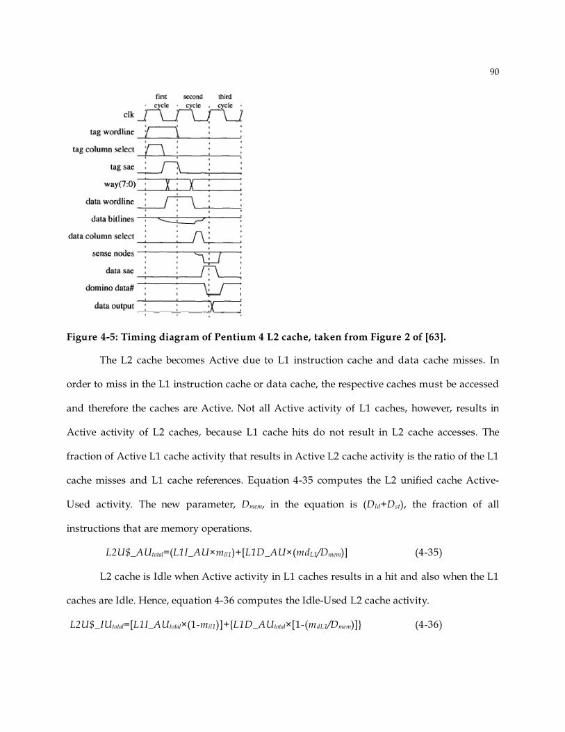
90

Figure 4-5: Timing diagram of Pentium 4 L2 cache, taken from Figure 2 of [63].

The L2 cache becomes Active due to L1 instruction cache and data cache misses. In

order to miss in the L1 instruction cache or data cache, the respective caches must be accessed

and therefore the caches are Active. Not all Active activity of L1 caches, however, results in

Active activity of L2 caches, because L1 cache hits do not result in L2 cache accesses. The

fraction of Active L1 cache activity that results in Active L2 cache activity is the ratio of the L1

cache misses and L1 cache references. Equation 4-35 computes the L2 unified cache Active-

Used activity. The new parameter, Dmem, in the equation is (Dld+Dst), the fraction of all

instructions that are memory operations.

L2U$_AUtotal=(L1I_AU×mil1)+[L1D_AU×(mdL1/Dmem)] (4-35)

L2 cache is Idle when Active activity in L1 caches results in a hit and also when the L1

caches are Idle. Hence, equation 4-36 computes the Idle-Used L2 cache activity.

L2U$_IUtotal=[L1I_AUtotal×(1-mil1)]+{L1D_AUtotal×[1-(mdL1/Dmem)]} (4-36)

91

+L1I_IUtotal+L1D_IUtotal

Equations 4-37 and 4-38 compute the Active-Flushed and Idle-Flushed L2 cache

activities, respectively. The flushed activities are derived by replacing Used activities in

equations 4-35 and 4-36 with the respective Flushed activities.

L2U$_AFtotal = (L1I_AFtotal×mil1) +[L1D_AFtotal×(mdL1/Dmem)] (4-37)

L2U$_IFtotal=[L1I_AFtotal×(1-mil1)]+{L1D_AFtotal×[1-(mdL1/Dmem)]}

+L1I_IFtotal+L1D_IFtotal

(4-38)

4.5.5 Main Memory

Main memory is Active when there is a miss in the L2 unified cache; otherwise the main

memory is Idle. In other words, the Active and Idle activities are related to the Active and Idle

activities of the L2 unified cache. Main memory can be Active only when a reference misses in

the L2 cache. For a reference to miss in the L2 cache, there has to be an L2 cache access and as

a result the L2 cache must be Active. Therefore, Active-Used main memory activity is

computed with equation 4-39 as a fraction of L2 cache Active-Used activity.

MM_AUtotal = L2U$_AU×[(mil2+mdl2)/(mil1+mdL1)] (4-39)

Main memory is Idle when the L2 cache is Idle and when the L2 cache is Active but the

L2 cache access does not result in a miss. Hence, equation 4-40 computes Idle-Used main

memory activity.

MM_IUtotal = {L2U$_AUtotal×{1-[(mil2+mdl2)/(mil1+mdL1)]}} + L2U$_IUtotal (4-40)

Active-Flushed and Idle-Flushed main memory activities are computed with formulas

in equations 4-41 and 4-42, respectively. The process of arriving the equations is the same one

employed to derive Used activities – all Used activities from equations 4-39 and 4-40 are

replaced with their respective Flushed activities.

92

MM_AFtotal = L2U$_AFtotal×[(mil2+mdl2)/(mil1+mdL1)] (4-41)

MM_IFtotal = {L2U$_AFtotal×{1-[(mil2+mdl2)/(mil1+mdL1)]}} + L2U$_IFtotal (4-42)

4.5.6 Physical Register File

The physical register file is accessed for the following two reasons: 1) for getting the

source operand data of an instruction. 2) for writing the destination operand data after

instruction execution. In the assumed generic superscalar processor the registers are read after

an instruction issues from the issue buffer.

Under ideal conditions the physical register file Active-Used activity is (i×Dreg) every

clock cycle, where Dreg is the number of registers accessed by an instruction on average. If

under ideal conditions, the program requires Cideal cycles to finish, the Active-Used activity for

the entire program is (Cideal×i×Dreg). Because Cideal = N×1/i, the formula in equation 4-43

calculates the Active-Used activity of the branch predictor.

PRF_AUideal = N×Dreg (4-43)

Under ideal conditions the physical register file is not accessed when instructions do not

require registers or require fewer registers than the available number of register file ports. If the

physical register file has Pprf ports and on average (i×Dreg) ports are Active, [Pprf-(i×Dreg)] is the

Idle physical register file activity every cycle. Equation 4-44 gives the Idle-Used physical

register file activity under ideal conditions.

PRF_IUideal = [(Pprf/i)-Dreg]×N (4-44)

When an instruction cache miss is being serviced, instruction issue stops for a number

of cycles equal to the miss penalty. As a result, there are no physical register file accesses, and

the Active-Used branch predictor activity during this time is zero. Equation 4-45 computes the

Idle-Used branch predictor activity because of an instruction cache miss.

93

PRF_IUimisses = N×Pprf×[(mil1×cl2)+(mil2×lmm)] (4-45)

When long data cache misses occur, instruction issue eventually stops. On average,

instruction issue stops for a number of cycles equal to the long data cache miss penalty. Recall

from equation 3-12 of Chapter 3 that the average miss penalty for a long data cache miss is

the miss delay divided by the number of overlapping misses on average. Therefore, the Idle-

Used physical register file activity due to long data cache misses is computed with equation 4-

46.

PRF_IUL2dmisses = N×Pprf×mdl2×(lmm/Novr) (4-46)

The total Active-Used activity is simply the Active-Used activity under ideal

conditions, given earlier in equation 4-43. The total Idle-Used activity is the summation of

equations 4-44, 4-45, and 4-46. Equation 4-47 has the formula for the total Idle-Used activity.

PRF_IUtotal=N×{[(Pprf/i)-Dreg]+[Pprf×((mil1×cl2)+(mil2×lmm))

+[Pprf×mdl2×(lmm/Novr)]}

(4-47)

The physical register file is on the miss-speculated path for cbr cycles including the Idle

cycles after a flush due to a branch misprediction. If the physical register file is in the jprfth stage

of the processor, the number of Idle cycles because of instruction re-fill after a misprediction

resolution is (jprf-1) cycles leading to [Pprf×(jprf-1)] Idle-Flushed L1 data cache activity.

For the remaining [cbr-(jprf-1)] miss-speculated cycles, the physical register file processes

miss-speculated instructions and therefore can be Active or Idle. Because the miss-speculated

instructions are assumed to have the same characteristics as the correct-path instructions, the

[cbr-(jprf-1)] cycles spent on processing miss-speculated instructions are Active and Idle in the

same proportion as the correct-path cycles.

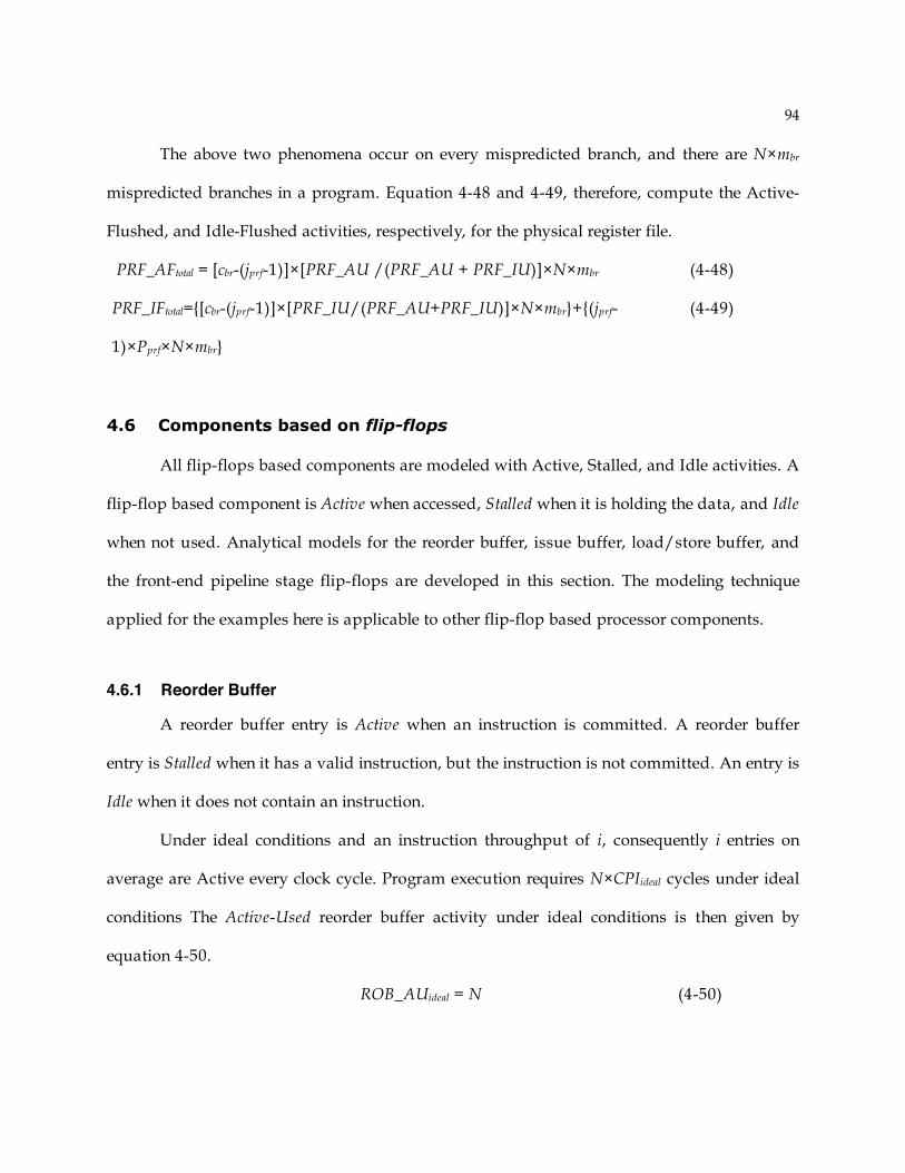
94

The above two phenomena occur on every mispredicted branch, and there are N×mbr

mispredicted branches in a program. Equation 4-48 and 4-49, therefore, compute the Active-

Flushed, and Idle-Flushed activities, respectively, for the physical register file.

PRF_AFtotal = [cbr-(jprf-1)]×[PRF_AU /(PRF_AU + PRF_IU)]×N×mbr (4-48)

PRF_IFtotal={[cbr-(jprf-1)]×[PRF_IU/(PRF_AU+PRF_IU)]×N×mbr}+{(jprf-

1)×Pprf×N×mbr}

(4-49)

4.6 Components based on flip-flops

All flip-flops based components are modeled with Active, Stalled, and Idle activities. A

flip-flop based component is Active when accessed, Stalled when it is holding the data, and Idle

when not used. Analytical models for the reorder buffer, issue buffer, load/store buffer, and

the front-end pipeline stage flip-flops are developed in this section. The modeling technique

applied for the examples here is applicable to other flip-flop based processor components.

4.6.1 Reorder Buffer

A reorder buffer entry is Active when an instruction is committed. A reorder buffer

entry is Stalled when it has a valid instruction, but the instruction is not committed. An entry is

Idle when it does not contain an instruction.

Under ideal conditions and an instruction throughput of i, consequently i entries on

average are Active every clock cycle. Program execution requires N×CPIideal cycles under ideal

conditions The Active-Used reorder buffer activity under ideal conditions is then given by

equation 4-50.

ROB_AUideal = N (4-50)

95

Because an average of i out of R entries commit every cycle, (R-i) reorder buffer entries

are Stalled. Equation 4-51 has the formula for Stalled-Used reorder buffer activity under ideal

conditions. Idle activity of reorder buffer is zero under ideal conditions.

ROB_SUideal = [(R/i)-1]×N (4-51)

When an instruction cache miss occurs, the reorder buffer drains. Instructions then

begin entering the reorder buffer after the miss penalty. Consequently, during this time all

reorder buffer entries are Idle; Active and Stall activities are both zero. Idle reorder buffer

activity is then computed with equation 4-52.

ROB_IUimisses = [(cl2×mil1)+(lmm×mil2)]×N×R (4-52)

During a long-data cache miss the load miss moves to the head of the reorder buffer

and instruction commit stops. Then the reorder buffer fills and dispatch stops. During the load

miss penalty, uncommitted instructions remain in the reorder buffer. Consequently, all reorder

buffer entries are Stalled; Active and Idle activities are both zero. Equation 4-53 then computes

the Stalled-Used reorder buffer activity because of long data cache misses.

ROB_SUL2dmisses = [(N×mdl2×lmm)/Novr]×R (4-53)

Reorder buffer has Active activity only under ideal conditions. Therefore the total

Active-Used activity is given by equation 4-50. Idle-Used reorder buffer activity is due to

instruction cache misses. There is no other factor contributing to reorder buffer’s Idle-Used

activity. Therefore, equation 4-52 computes the total Idle-Used reorder buffer activity. The

total Stall-Used activity is the sum of equations 4-51 and 4-53, and is given in equation 4-54.

ROB_SUtotal = N×R×{[(1/i)-1]+[(mdl2×lmm)/Novr]} (4-54)

After every branch misprediction, the reorder buffer experiences cbr miss-speculated

cycles. Out of cbr cycles, (jdis-1) are Idle cycles because following the pipeline flush, all reorder

buffer entries are Idle, where jdis is the number of pipeline stages of the dispatch logic.

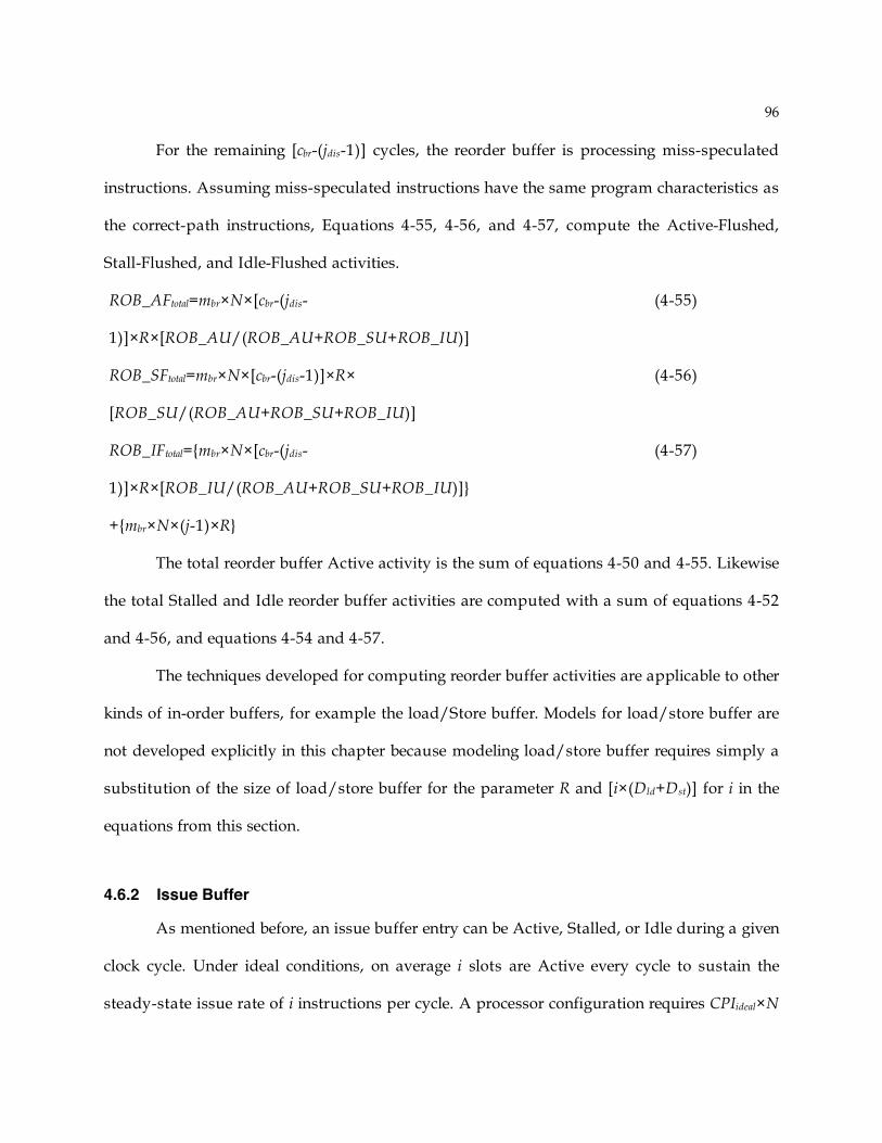
96

For the remaining [cbr-(jdis-1)] cycles, the reorder buffer is processing miss-speculated

instructions. Assuming miss-speculated instructions have the same program characteristics as

the correct-path instructions, Equations 4-55, 4-56, and 4-57, compute the Active-Flushed,

Stall-Flushed, and Idle-Flushed activities.

ROB_AFtotal=mbr×N×[cbr-(jdis-

1)]×R×[ROB_AU/(ROB_AU+ROB_SU+ROB_IU)]

(4-55)

ROB_SFtotal=mbr×N×[cbr-(jdis-1)]×R×

[ROB_SU/(ROB_AU+ROB_SU+ROB_IU)]

(4-56)

ROB_IFtotal={mbr×N×[cbr-(jdis-

1)]×R×[ROB_IU/(ROB_AU+ROB_SU+ROB_IU)]}

+{mbr×N×(j-1)×R}

(4-57)

The total reorder buffer Active activity is the sum of equations 4-50 and 4-55. Likewise

the total Stalled and Idle reorder buffer activities are computed with a sum of equations 4-52

and 4-56, and equations 4-54 and 4-57.

The techniques developed for computing reorder buffer activities are applicable to other

kinds of in-order buffers, for example the load/Store buffer. Models for load/store buffer are

not developed explicitly in this chapter because modeling load/store buffer requires simply a

substitution of the size of load/store buffer for the parameter R and [i×(Dld+Dst)] for i in the

equations from this section.

4.6.2 Issue Buffer

As mentioned before, an issue buffer entry can be Active, Stalled, or Idle during a given

clock cycle. Under ideal conditions, on average i slots are Active every cycle to sustain the

steady-state issue rate of i instructions per cycle. A processor configuration requires CPIideal×N

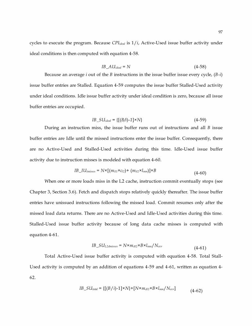
97

cycles to execute the program. Because CPIideal is 1/i, Active-Used issue buffer activity under

ideal conditions is then computed with equation 4-58.

IB_AUideal = N (4-58)

Because an average i out of the B instructions in the issue buffer issue every cycle, (B-i)

issue buffer entries are Stalled. Equation 4-59 computes the issue buffer Stalled-Used activity

under ideal conditions. Idle issue buffer activity under ideal condition is zero, because all issue

buffer entries are occupied.

IB_SUideal = {[(B/i)-1]×N} (4-59)

During an instruction miss, the issue buffer runs out of instructions and all B issue

buffer entries are Idle until the missed instructions enter the issue buffer. Consequently, there

are no Active-Used and Stalled-Used activities during this time. Idle-Used issue buffer

activity due to instruction misses is modeled with equation 4-60.

IB_IUimisses = N×[(mil1×cl2)+ (mil2×lmm)]×B (4-60)

When one or more loads miss in the L2 cache, instruction commit eventually stops (see

Chapter 3, Section 3.6). Fetch and dispatch stops relatively quickly thereafter. The issue buffer

entries have unissued instructions following the missed load. Commit resumes only after the

missed load data returns. There are no Active-Used and Idle-Used activities during this time.

Stalled-Used issue buffer activity because of long data cache misses is computed with

equation 4-61.

IB_SUL2dmisses = N×mdl2×B×lmm/Novr (4-61)

Total Active-Used issue buffer activity is computed with equation 4-58. Total Stall-

Used activity is computed by an addition of equations 4-59 and 4-61, written as equation 4-

62.

IB_SUtotal = {[(B/i)-1]×N}+[N×mdl2×B×lmm/Novr] (4-62)

98

Total Idle-Used activity is computed with equation 4-60.

Due to each branch misprediction, the issue buffer experiences cbr miss-speculated

cycles. Out of the cbr cycles, (jdis-1) are Idle cycles because following the pipeline flush, all issue

buffer entries are Idle, where jdis is the depth of the dispatch stage.

For the remaining [cbr-(jdis-1)] cycles, the issue buffer is processing miss-speculated

instructions. Equations 4-64, 4-65, and 4-66 compute the Active-Flushed, Stall-Flushed, and

Idle-Flushed activities.

IB_AFtotal = (mbr×N×B)×[cbr-( jdis -1)]×[IB_AU/(IB_AU+IB_SU+IB_IU)] (4-64)

IB_SFtotal = (mbr×N×B)×[cbr-( jdis -1)]×[IB_SU/(IB_AU+IB_SU+IB_IU)] (4-65)

IB_IFtotal = {(mbr×N×B)×[cbr-( jdis -1)]×[IB_IU/(IB_AU+IB_SU+IB_IU)]}

+ {(jdis-1)×mbr×N×B }

(4-66)

4.6.3 Pipeline stage flip-flops

Every pipeline stage has flip-flops that synchronize that stage with its neighboring

stages (see Figures 4-2 and 4-4). A single pipeline stage flip-flop is Active if the combinational

logic in that stage is performing its intended operation and the following cycle the contents are

transferred to the flip-flop of the pipeline stage. A single front-end pipeline stage is Stalled if

the flip-flops feeding the combinational logic are holding the data and the combination logic is

not performing its intended operation. A single front-end pipeline stage is Idle if the stage does

not have valid information to process. In this case, for a clock-gated design, the flip-flops

feeding the pipeline stage can be clock-gated.

When there are no cache misses and branch mispredictions the processor issues

instructions at the steady-state rate. The pipeline stage flip-flops receive instruction/data from

the previous stage. The instruction/data is processed and then sent to the subsequent pipeline

99

stage at the end of the clock cycle. This process is performed at the steady-state issue rate, and

therefore the pipeline stage has Active-Used activity of i every clock cycle, on average.

Equation 4-64 gives the Active-Used pipeline stage activity for the entire program.

FE_AUideal = N (4-64)

A pipeline stage flip-flop is Idle if it is not occupied by an instruction; under ideal

conditions this can happen due to taken branches. For example, if a front-end pipeline stage

can process at the peak four instructions every clock cycle, but only three instructions are

processed because of taken branches, 3/4ths of the stage is Idle. In general, Idle activity of a

pipeline stage under ideal conditions is (I-i) every cycle. Equation 4-66 gives the Idle-Used

activity under ideal conditions for executing the entire program.

FE_IUideal = [(I/i)-1]×N (4-66)

When there is an instruction cache miss, the front-end pipeline ultimately becomes

empty and contains no valid instructions. Equation 4-67 is the formula for computing Idle

activity of a pipeline stage because of instruction cache misses.

FE_IUimisses = I×N×[(mil1×cl2)+(mil2×lmm)] (4-67)

When there is a data cache miss that goes all the way to the main memory the front-end

pipeline stages stall for the miss penalty cycles. Equation 4-68 gives the Stalled-Used activity

because of long data cache misses.

FE_SUL2dmisses = i×N×mdl2×(lmm/Novr) (4-68)

During a long data cache miss, a front-end pipeline stage can be Idle because of the

available instruction slots that are not occupied. Equation 4-69 is the formula for the Idle-

Used activity of front-end pipeline stage due to long data cache misses.

FE_IUL2dmisses = (I-i)×N×mdl2×(lmm/Novr) (4-69)

100

Total Active-Used pipeline stage activity, denoted as FE_AUtotal, is computed with

equation 4-64, because instruction cache misses and long data cache misses do not cause

additional Active activity. Total Stalled-Used activity, denoted as FE_SUtotal, is computed with

equation 4-68. Total Idle-Used activity, denoted as FE_IUtotal, is computed with a summation

of equations 4-66, 4-67, and 4-69.

Because of a misprediction every pipeline stage experiences cbr miss-speculated cycles.

Out of the cbr cycles, stage at depth jstg has (jstg-1) Idle cycles; [cbr-(jstg-1)] cycles are spent

processing miss-speculated instructions. Active, Stalled, and Idle activities for [cbr-(jstg-1)]

miss-speculated cycles is proportional to the Active, Stalled, and Idle activities for the correct-

path cycles. Equations 4-70, 4-71, and 4-72, calculate Active-Flushed, Stalled-Flushed, and

Idle-Flushed activities, respectively, for the flip-flops in pipeline stage jstg.

FF_AFtotal=(mbr×N×I)×[cbr-(jstg-1)]

×[FF_AUtotal/(FF_AUtotal+FF_SUtotal+FF_IUtotal)]

(4-70)

FF_SFtotal=(mbr×N×I)×[cbr-(jstg-1)]

×[FF_SUtotal/(FF_AUtotal+FF_SUtotal+FF_IUtotal)]

(4-71)

FF_IFtotal={(mbr×N×I)×[cbr-(jstg-1)]

×[FF_IUtotal/(FF_AUtotal+FF_SUtotal+FF_IUtotal)]}+ {( jstg-1)×mbr×N×I}

(4-72)

4.7 Analytical Model Evaluation

All the parts of the first-order energy activity model are now complete. The cycle-

accurate simulation based method developed earlier and validated in Section 4.2 is used as the

reference for evaluating the accuracy of the analytical model. The analytical energy activity

model is evaluated by comparing its energy per instruction (EPI) estimates with the cycle-

accurate simulation EPI estimates.

101

PowerPC440-like and Power4-like baseline designs are used for the comparing the EPI

estimates from cycle-accurate simulation and the analytical model. PowerPC440-like baseline

processor has five front-end pipeline stages, an issue width of two, a reorder buffer of 64

entries and an issue buffer of 48 entries. The instruction and data caches are 2K 4-way set

associative with 64 bytes per cache line; a unified 32K L2 cache is 4-way set-associative with

64 byte lines, and the branch predictor is 2K gShare. The caches and branch predictor are

intentionally much smaller than those used in PowerPC440. Smaller caches and branch

predictor stress the model by increasing the chances of miss-event overlaps.

The Power4-like baseline processor has 11 front-end pipeline stages, an issue width of

four, a reorder buffer of 256 entries and an issue buffer of 128 entries. The instruction and data

caches are 4K 4-way set associative with 128 bytes per cache line; a unified 512K L2 cache is 8-

way set-associative with 128 byte lines, and the branch predictor is 16K gShare. Similar to the

PowerPC440-like baseline, the Power4-like baseline has smaller caches than those used in the

actual Power4 implementation[44, 45].

The energy activity multipliers for computing the energy come from the energy

multiplier library provided in Wattch. The important thing is that the same energy activity

multipliers are used for both the analytical energy activity model and for the activities

generated with cycle-accurate simulation. Therefore, a deviation in the EPI indicates a

deviation in the energy activities.

4.7.1 Evaluation Metrics

The same two metrics, correlation coefficient and histogram of differences, used for

evaluating the analytical CPI model in Section 3.7 of Chapter 3 are employed here to evaluate

102

the analytical energy activity model. For continuity the two metrics are summarized below.

Detailed discussion of these metrics is in Chapter 3.

• The correlation coefficient is a number between zero and one that tells how closely

the analytical model and simulation track each other.

• The Histogram of differences between the analytical model and simulation

estimates is useful because differences with a Normal distribution means that

the first-order model can be used for making a relative comparison of two or

more superscalar designs for choosing the Pareto-optimal designs.

4.7.2 Correlation between analytical model and simulation

The correlation between the analytical model and cycle-accurate simulation is

demonstrated in Figure 4-6. In the figure, the x-axis is the EPI generated from simulation and

the y-axis is the EPI computed with the analytical energy activity model. The diamonds

represent the observed correlation between the two models for all 35 benchmarks and the two

baseline designs. The correlation coefficient is 0.99. The analytical energy activity model tracks

cycle-accurate simulation very well can be used for making tradeoffs between two or more

designs during the Pareto-optimal search.

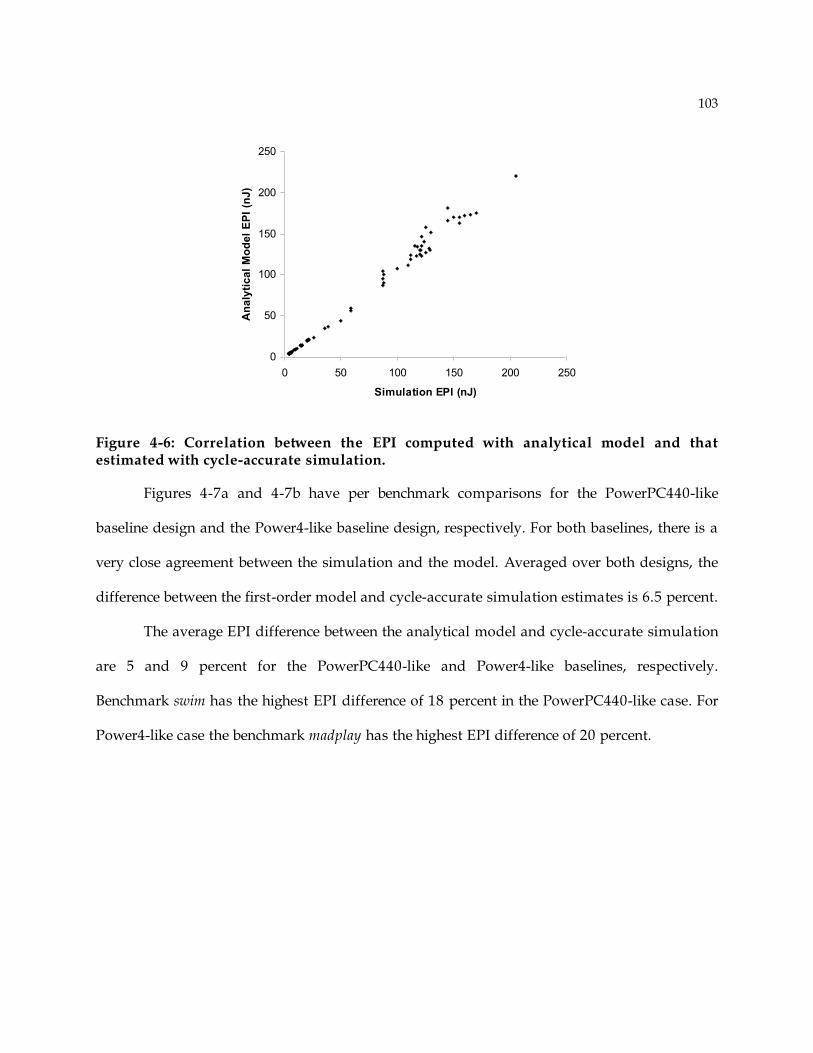
103

0

50

100

150

200

250

0 50 100 150 200 250

Simulation EPI (nJ)

An

aly

tic

al

Mo

de

l E

PI

(nJ

)

Figure 4-6: Correlation between the EPI computed with analytical model and that estimated with cycle-accurate simulation.

Figures 4-7a and 4-7b have per benchmark comparisons for the PowerPC440-like

baseline design and the Power4-like baseline design, respectively. For both baselines, there is a

very close agreement between the simulation and the model. Averaged over both designs, the

difference between the first-order model and cycle-accurate simulation estimates is 6.5 percent.

The average EPI difference between the analytical model and cycle-accurate simulation

are 5 and 9 percent for the PowerPC440-like and Power4-like baselines, respectively.

Benchmark swim has the highest EPI difference of 18 percent in the PowerPC440-like case. For

Power4-like case the benchmark madplay has the highest EPI difference of 20 percent.

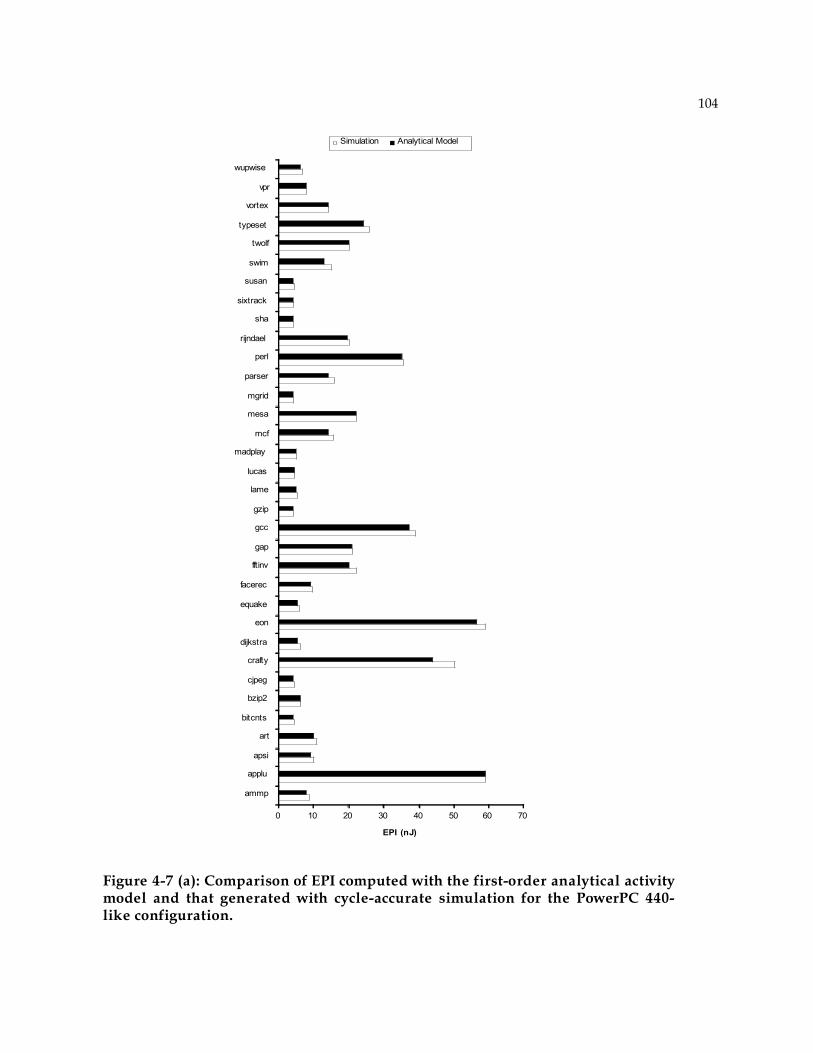
104

0 10 20 30 40 50 60 70

ammp

applu

apsi

art

bitcnts

bzip2

cjpeg

crafty

dijkstra

eon

equake

facerec

fftinv

gap

gcc

gzip

lame

lucas

madplay

mcf

mesa

mgrid

parser

perl

rijndael

sha

sixtrack

susan

swim

twolf

typeset

vortex

vpr

wupwise

EPI (nJ)

Simulation Analytical Model

Figure 4-7 (a): Comparison of EPI computed with the first-order analytical activity model and that generated with cycle-accurate simulation for the PowerPC 440-like configuration.

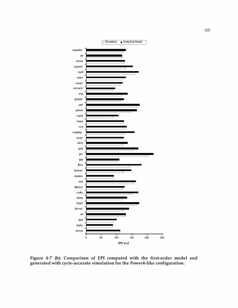
105

0 50 100 150 200 250

ammp

applu

apsi

art

bitcnts

bzip2

cjpeg

crafty

dijkstra

eon

equake

facerec

fftinv

gap

gcc

gzip

lame

lucas

madplay

mcf

mesa

mgrid

parser

perl

rijndael

sha

sixtrack

susan

swim

twolf

typeset

vortex

vpr

wupwise

EPI (nJ)

Simulation Analytical Model

Figure 4-7 (b): Comparison of EPI computed with the first-order model and generated with cycle-accurate simulation for the Power4-like configuration.

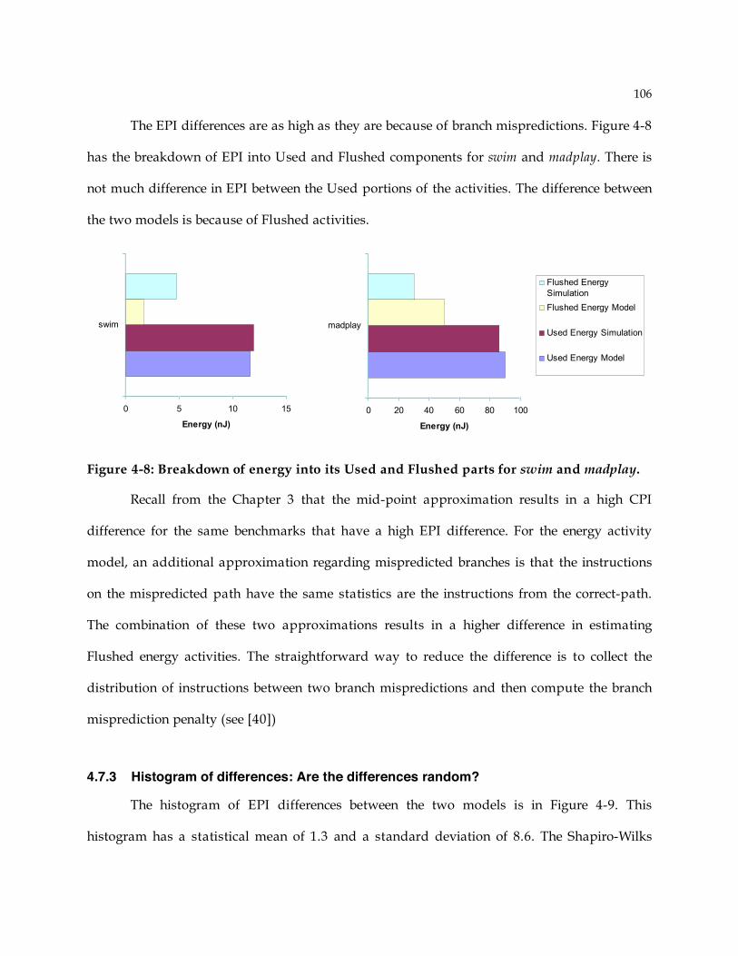
106

The EPI differences are as high as they are because of branch mispredictions. Figure 4-8

has the breakdown of EPI into Used and Flushed components for swim and madplay. There is

not much difference in EPI between the Used portions of the activities. The difference between

the two models is because of Flushed activities.

0 5 10 15

swim

Energy (nJ)

0 20 40 60 80 100

madplay

Energy (nJ)

Flushed Energy

Simulation

Flushed Energy Model

Used Energy Simulation

Used Energy Model

Figure 4-8: Breakdown of energy into its Used and Flushed parts for swim and madplay.

Recall from the Chapter 3 that the mid-point approximation results in a high CPI

difference for the same benchmarks that have a high EPI difference. For the energy activity

model, an additional approximation regarding mispredicted branches is that the instructions

on the mispredicted path have the same statistics are the instructions from the correct-path.

The combination of these two approximations results in a higher difference in estimating

Flushed energy activities. The straightforward way to reduce the difference is to collect the

distribution of instructions between two branch mispredictions and then compute the branch

misprediction penalty (see [40])

4.7.3 Histogram of differences: Are the differences random?

The histogram of EPI differences between the two models is in Figure 4-9. This

histogram has a statistical mean of 1.3 and a standard deviation of 8.6. The Shapiro-Wilks

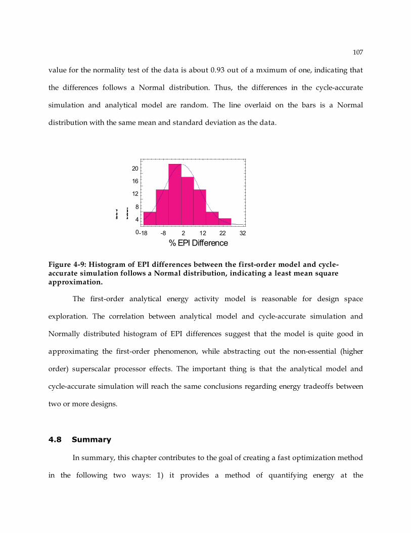
107

value for the normality test of the data is about 0.93 out of a mximum of one, indicating that

the differences follows a Normal distribution. Thus, the differences in the cycle-accurate

simulation and analytical model are random. The line overlaid on the bars is a Normal

distribution with the same mean and standard deviation as the data.

-18 -8 2 12 22 32

% EPI Difference

0

4

8

12

16

20

Figure 4-9: Histogram of EPI differences between the first-order model and cycle-accurate simulation follows a Normal distribution, indicating a least mean square approximation.

The first-order analytical energy activity model is reasonable for design space

exploration. The correlation between analytical model and cycle-accurate simulation and

Normally distributed histogram of EPI differences suggest that the model is quite good in

approximating the first-order phenomenon, while abstracting out the non-essential (higher

order) superscalar processor effects. The important thing is that the analytical model and

cycle-accurate simulation will reach the same conclusions regarding energy tradeoffs between

two or more designs.

4.8 Summary

In summary, this chapter contributes to the goal of creating a fast optimization method

in the following two ways: 1) it provides a method of quantifying energy at the

108

microarchitecture level with the Active, Stall, and Idle activities, and 2) it provides an

analytical method for computing the Active, Stall, and Idle activities.

The ASI method provides a view of energy consumption from the microarchitecture

perspective. This method is based on the operational principles of fundamental building block

of microprocessors. Additionally, the ASI method is more precise and provides more insight

than the conventional utilization method. This provides the ability to reason and reduce energy

consumption using microarchitecture innovations.

The analytical model for computing ASI activities establishes a cause-and-effect

relationship between superscalar processor microarchitecture, program characteristics, and

energy activities. The analytical approach of computing and EPI value using ASI activities is

based on the same fundamental principles of superscalar processors as the CPI model from

previous chapter. Overall, the analytical model estimates and cycle-accurate simulation

estimates have a correlation coefficient of 0.99 and are on average 8 percent of each other. As it

will become evident in the next chapter, the precision and speed of analytical energy activity

model and the analytical CPI model (Chapter 3) allows finding the Pareto-optimal

configurations orders of magnitude faster than cycle-accurate simulation exhaustive search

and cycle-accurate simulation-based simulated annealing.

109

Chapter 5: Search Method

The previous two chapters developed analytical methods for estimating CPI and EPI of

a program running on a parameterized microarchitecture configuration. This chapter develops

a search method for finding the Pareto-optimal configurations. This search method uses the

CPI and energy activity models developed in Chapters 3 and 4, respectively.

5.1 Overview of the Search Method

The proposed search method decomposes the superscalar processor into pipelines,

caches, and branch predictor and then applies a divide-and-conquer strategy. Insights from the

CPI and EPI models suggest that the effects of miss-events on CPI and EPI can be analyzed

independently, in isolation of each other. Furthermore, total superscalar processor area is the

sum of the areas of individual sub-systems, by definition. In general, when systems have this

additive property the individual components can be optimized independently [64].

The overall optimization algorithm consists of the following five steps.

1. Software Evaluation: For the given application program(s), measure miss rates for all

instruction caches, data caches, unified caches, and branch predictors in the design space

with simple, one-time trace-driven simulations.

2. Cache Optimization: Find miss-rate, energy per access, and area Pareto-optimal cache

designs from the set of caches evaluated in Step 1. Miss-rates are determined in Step 1. The

area and energy per access information is obtained from the component database.

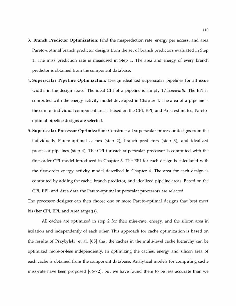
110

3. Branch Predictor Optimization: Find the misprediction rate, energy per access, and area

Pareto-optimal branch predictor designs from the set of branch predictors evaluated in Step

1. The miss prediction rate is measured in Step 1. The area and energy of every branch

predictor is obtained from the component database.

4. Superscalar Pipeline Optimization: Design idealized superscalar pipelines for all issue

widths in the design space. The ideal CPI of a pipeline is simply 1/issuewidth. The EPI is

computed with the energy activity model developed in Chapter 4. The area of a pipeline is

the sum of individual component areas. Based on the CPI, EPI, and Area estimates, Pareto-

optimal pipeline designs are selected.

5. Superscalar Processor Optimization: Construct all superscalar processor designs from the

individually Pareto-optimal caches (step 2), branch predictors (step 3), and idealized

processor pipelines (step 4). The CPI for each superscalar processor is computed with the

first-order CPI model introduced in Chapter 3. The EPI for each design is calculated with

the first-order energy activity model described in Chapter 4. The area for each design is

computed by adding the cache, branch predictor, and idealized pipeline areas. Based on the

CPI, EPI, and Area data the Pareto-optimal superscalar processors are selected.

The processor designer can then choose one or more Pareto-optimal designs that best meet

his/her CPI, EPI, and Area target(s).

All caches are optimized in step 2 for their miss-rate, energy, and the silicon area in

isolation and independently of each other. This approach for cache optimization is based on

the results of Przybylski, et al. [65] that the caches in the multi-level cache hierarchy can be

optimized more-or-less independently. In optimizing the caches, energy and silicon area of

each cache is obtained from the component database. Analytical models for computing cache

miss-rate have been proposed [66-72], but we have found them to be less accurate than we

111

would like. As a result, we use a trace-driven cache simulator, Tycho[73], to evaluate cache

performance. The rationale for using Tycho is that it implements the fastest general algorithm

called the all-associative algorithm[74] for simultaneously measuring cache miss-rates of

several caches.

Unlike caches, the branch predictors do not have the inclusion property. Consequently,

branch predictors (step 3) in the component database are analyzed one at a time with trace-

driven simulations.

The superscalar pipeline by itself has numerous parameters such as the number of

integer arithmetic and logic-units, floating-point adders, number of reorder buffer entries, and

number of issue buffer entries. Enumerating through various choices for each parameter can

become computationally expensive. Consequently, a computationally simple, direct method is

used in step 4 for finding Pareto-optimal superscalar pipelines. This method is the focus of the

next section.

5.2 Superscalar Pipeline Optimization

The superscalar pipeline optimization process is based on the observations and results

from previous work regarding the relationship between inherent program parallelism and the

parallelism that can be extracted with out-of-order superscalar processors. Noonburg and

Shen [36], Jouppi [75], and Theobald, et al. [76] found that under ideal conditions, in a

balanced superscalar processor, the parallelism available from the application software is close

(if not equal) to the upper bound on the parallelism that the processor can extract.

In the superscalar processor used in this dissertation (see Figure 1-1) the upper bound

on the parallelism that can be extracted from the program is set by the issue width I. The

superscalar pipeline optimization process therefore selects processor resources such that I is

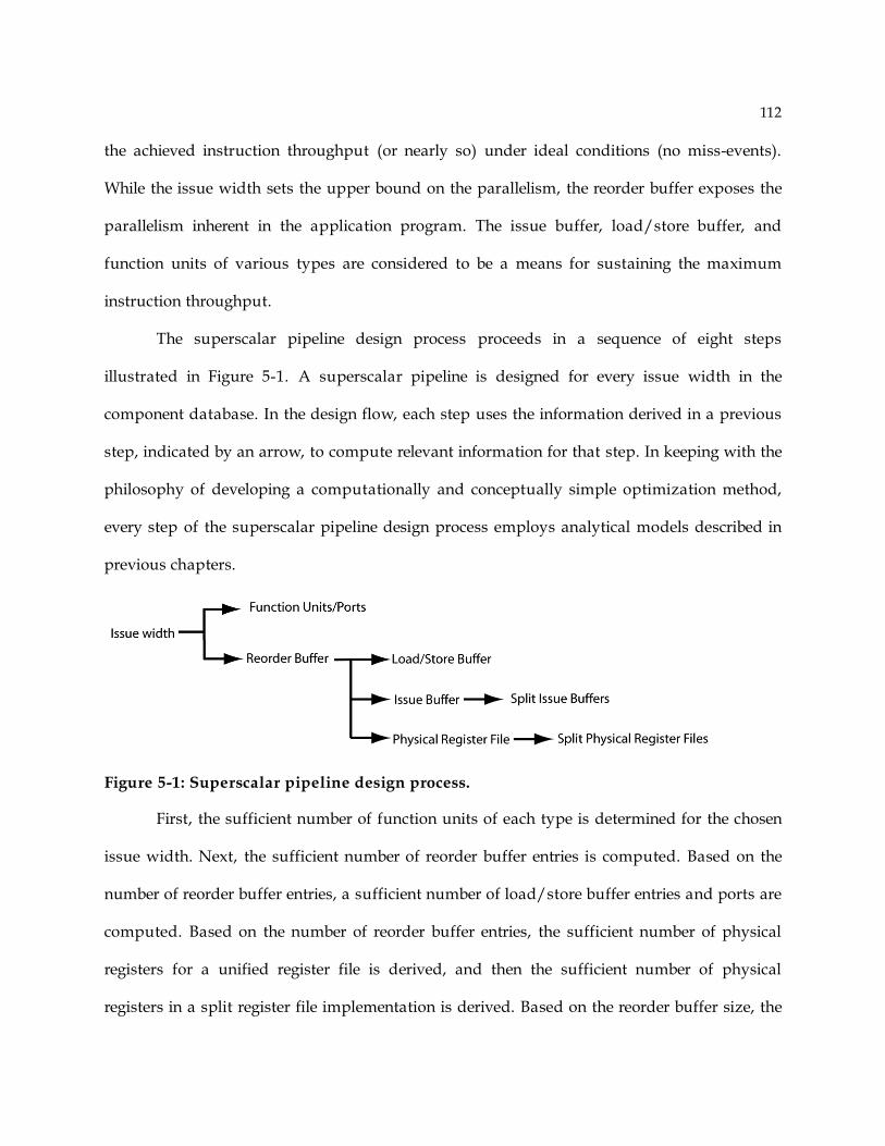
112

the achieved instruction throughput (or nearly so) under ideal conditions (no miss-events).

While the issue width sets the upper bound on the parallelism, the reorder buffer exposes the

parallelism inherent in the application program. The issue buffer, load/store buffer, and

function units of various types are considered to be a means for sustaining the maximum

instruction throughput.

The superscalar pipeline design process proceeds in a sequence of eight steps

illustrated in Figure 5-1. A superscalar pipeline is designed for every issue width in the

component database. In the design flow, each step uses the information derived in a previous

step, indicated by an arrow, to compute relevant information for that step. In keeping with the

philosophy of developing a computationally and conceptually simple optimization method,

every step of the superscalar pipeline design process employs analytical models described in

previous chapters.

Figure 5-1: Superscalar pipeline design process.

First, the sufficient number of function units of each type is determined for the chosen

issue width. Next, the sufficient number of reorder buffer entries is computed. Based on the

number of reorder buffer entries, a sufficient number of load/store buffer entries and ports are

computed. Based on the number of reorder buffer entries, the sufficient number of physical

registers for a unified register file is derived, and then the sufficient number of physical

registers in a split register file implementation is derived. Based on the reorder buffer size, the

113

number of unified issue buffer entries is computed. The issue width and sufficient entries for a

split issue buffer can then be derived.

Other design dimensions, such as the fetch, dispatch, decode, and commit widths, are

not explicitly shown in Figure 5-1 and are assumed to increase linearly with the issue width.

For example, if the issue width is four, four decoders are required to sustain the peak issue

rate every cycle.

Step 1: Determine the sufficient number of function units

Given the peak issue rate of I, the processor must have an adequate number of

functions units of each type in order to at the least satisfy the mean throughput requirements.

As a rough approximation the number of units can be computed as ( )h hI D Y! ! , where Dh is

the fraction of instructions require the function unit of type h, and Yh is the issue latency of

that function unit (issue latency = 1 if the unit is fully pipelined). In practice, however,

instructions that require a function unit of type h can occur in bursts, where the short-term

demand is significantly higher than the mean requirement Dh. Consequently, the number of

function units must be sufficient to accommodate the bursts in function unit demand, not just

the long-term average demand..

One way to model bursts in the function unit demand is to view it as the classic

counting-with-replacement problem[77]. The bursts can then be modeled as a Binomial

random variable Xh with mean ( )hI D! and variance ( )( )1h h

I D D! ! " . An exact expression

for the probability of bursts of size k denoted as P(Xh = k) is:

( ) ( )( )

!1 , where

! !

I kk

h h h

I I IP X k D D

k k k I k

!" # " #= = ! =$ % $ % !& ' & '

(5-1)

114

The Binomial random variable approximation was validated with the cycle-accurate

simulation experiments for issue widths of 2, 4, 8, and 16. Through the cycle-accurate

simulations the probabilities for instruction issue groups of specific function unit types were

measured. Next, through instruction trace analysis values of Dh were collected for a total of 16

types of instructions. Then using the Dh values from trace analysis and assuming a Binomial

distribution, the probabilities for bursts of various sizes were computed. Finally, the root-

mean-square (RMS) error between the analytically computed distribution and the cycle-

accurate simulation generated distribution was calculated for each type of function unit and

every simulated issue width. The highest RMS error was 0.04 for the benchmark crafty with

issue width 16. The highest RMS error by itself is a small value (close to zero) indicating that

Binomial distribution models bursts in the demand for function units.

Therefore, the sufficient number of function units of a specific type can be determined

by evaluating the Binomial distribution for k = 0, 1, …, I. Then the value of k at the knee of the

Binomial distribution is chosen as the sufficient number of units. This process however does

not yield an elegant, closed form equation.

To arrive at a closed form equation, the Binomial distribution that has a mean ( )hI D!

and variance ( )1h h

I D D! " is approximated with the Normal distribution that has a mean

( )hI D! and variance ( )1h h

I D D! " , by the virtue of the Central Limit Theorem [49]. The

sufficient number of function units can then be computed by choosing the number of bursts at

the knee of the Normal distribution. The knee of the curve of a Normal distribution can be

computed with a closed form expression by adding two standard deviations to its mean as:

( )( )2 1h h h

I D I D D! + ! ! " .

115

One caveat with the Normal distribution is that it is continuous while the Binomial

distribution is discrete. As a result the continuity correction [49] must be applied by ceiling the

number of function units at ( )hI D! . The formula for the sufficient number of function units

of type h with the continuity correction is given as equation 5-2.

( )( ) ( )( )2 1min ,h h h h h hF I D I D D Y I Y! "= # + # # $ # #% &% &

(5-2)

Step 2: Determine the sufficient number of reorder buffer entries

The sufficient number of reorder buffer entries is derived using the iW characteristic

introduced in Chapter 3. As previously mentioned, the iW characteristic models the

relationship between the achieved issue rate and the reorder buffer size (see Figure 3-4 from

Chapter 3). The sufficient number of reorder buffer entries, denoted as R, is selected as the

smallest number of entries that achieves an issue rate within 2.5 percent of the issue width. The

design point is chosen at 2.5 percent because the slope of the Normal distribution’s cumulative

distribution function starts to flatten at 97.5 percent.

Step 3: Determine the sufficient number of load/store buffer entries

The load/store buffer can be viewed as a reorder buffer specifically for memory

instructions – it holds all in-flight load and store instructions in program order. The number of

load/store buffer entries is computed with equation 5-3, where Dmem is the fraction of

instructions that are loads and stores.

( ) ( )( )( )min 2 1 ,! "= # + # # $% &% &mem mem memLS R D R D D R (5-3)

116

Equation 5-3 has the same form as that of equation 5-1 used for computing the

number of various types of function units. The rationale is that deriving the number of entries

load/store buffer entries are conceptually the same as those employed to derive various types

of function units. The term ( )memR D! in equation 5-3 models the fact that the load/store

buffer must have at the least number of entries equal to the average fraction of the in-flight

instructions in the program. The term ( )( )2 1! ! "mem mem

R D D computes the additional

load/store buffer entries required to sustain the peak issue rate when load and store

instructions are dispatched in bursts.

The number of issue ports for the load/store buffer (the same as the read and write

ports for the data cache) is computed with equation 5-4. Here the unified issue width I is used

to derive the specific issue width for the load/store buffer.

( ) ( )( )( )min 2 1 ,! "= # + # # $% &% &LS mem mem memI I D I D D I (5-4)

Step 4: Determine the sufficient number of physical registers

The physical register file must have sufficient registers to accommodate the

requirements of all in-flight instructions that write to a register. The processor must have at

least as many physical registers as the number of architected registers in the ISA. Today,

embedded-, desktop-, and server-class microprocessors all have a separate physical register

file for integer and floating-point instructions [3, 4, 44, 78, 79]. Consequently, the focus here is

on computing the sufficient number of physical registers for an implementation that has

separate register files.

Let us denote the fraction of instructions that write to a physical register and are of

type h as Dwr,h. Recall that the number of in-flight instructions in the reorder buffer size was

117

previously denoted as R. The sufficient number of physical registers for a physical register file

of type h can then be computed as:

( ) ( )( )2 1, , ,

min ,h wr h wr h wr h

PR R D R D D R! "# $= % + % % &' () *) *+ ,

(5-5)

Step 5: Determine the sufficient number of issue buffer entries

The issue buffer holds a subset of the instructions that have dispatched, but not issued.

These instructions are a subset of all in-flight instructions that are present in the reorder buffer.

The sufficient number of issue buffer entries is computed using Little’s Law as the product of

the average number of cycles an instruction waits in the issue buffer and the instruction

issue/dispatch rate.

First, assuming unit latency instructions, an instruction waits in the issue buffer for

A(R) cycles on average, where R is the number of in-flight instructions set by the reorder buffer

size, and the function A( ) gives the number of instructions on the dependence chain that

provide data to a subject instruction averaged over all R instructions. Function A( ) is the

produced as a by-product while measuring the longest instruction dependence statistic (see

Chapter 3, Section 3.2).

With more realistic, non-unit execution latencies, the number of cycles an instruction

waits in the issue buffer increases relative to the unit latency case. Figure 5-2 illustrates how

non-unit execution latencies affect the average number of cycles an instruction waits in the

issue buffer. There are two dependence chains shown in the figure. The black filled circles

represent instructions and arrows represent data dependence from one instruction to another.

The number on top of each instruction denotes the number of cycles the instruction will wait in

the issue buffer. The dependence chain on the top depicts the unit latency case. The

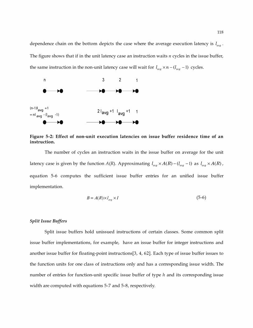
118

dependence chain on the bottom depicts the case where the average execution latency is avgl .

The figure shows that if in the unit latency case an instruction waits n cycles in the issue buffer,

the same instruction in the non-unit latency case will wait for 1( )avg avgl n l! " " cycles.

Figure 5-2: Effect of non-unit execution latencies on issue buffer residence time of an instruction.

The number of cycles an instruction waits in the issue buffer on average for the unit

latency case is given by the function A(R). Approximating 1( ) ( )avg avgl A R l! " " as ( )avgl A R! ,

equation 5-6 computes the sufficient issue buffer entries for an unified issue buffer

implementation.

( )= ! !avgB A R l I (5-6)

Split Issue Buffers

Split issue buffers hold unissued instructions of certain classes. Some common split

issue buffer implementations, for example, have an issue buffer for integer instructions and

another issue buffer for floating-point instructions[3, 4, 62]. Each type of issue buffer issues to

the function units for one class of instructions only and has a corresponding issue width. The

number of entries for function-unit specific issue buffer of type h and its corresponding issue

width are computed with equations 5-7 and 5-8, respectively.

119

( )( )( )min 2 1 ,! "= # + $% &% &h h h h

B B D D D B

(5-7)

( )( )( )2 1! "= # + $% &% &min ,

h h h hI I D D D I

(5-8)

5.3 Evaluation of the proposed Design Optimization method

The development of the search process for finding Pareto-optimal superscalar

processors is now complete. The search process, coupled with the CPI and energy activity

models developed in Chapters 3 and 4, encompass the analytical design optimization method.

This section evaluates the proposed design optimization method by comparing it to the

baseline method and a conventional multi-objective optimization method based on a heuristic

algorithm.

The analytical method uses the process described in Section 5.1. The baseline method

evaluates all available design alternatives with cycle-accurate simulations and then chooses the

Pareto-optimal configurations.

For comparisons, the conventional multi-objective method uses the popular constraint

approach and converts the multi-objective optimization problem to a single-objective

optimization problem[80, 81]. This is done by first fixing EPI and Area at some values. Then,

the single-objective optimization problem is solved with Simulated Annealing in order to

minimize the CPI for the target EPI and Area. This process is then repeated for all available

EPI and Area combinations, yielding a set of Pareto-optimal design in terms of CPI-EPI-Area.

Simulated Annealing is the chosen heuristic for two reasons. (1) It is the most widely

used optimization method. (2) Simulated Annealing has theoretical basis that guarantees a

global optimal design given unbounded resources.

120

5.3.1 Evaluation Metrics

The following four metrics are used for the comparison: coverage, false positives,

correlation of Pareto-optimal curves, and time complexity. Each metric is described below.

• Coverage is the fraction of the designs in the Pareto-optimal set generated with the baseline

method that are also in the Pareto-optimal set generated with the subject method.

• False positives is the fraction of the designs in the Pareto-optimal sets generated by the

subject method that are not in the Pareto-optimal set generated by the baseline method.

• Correlation of Pareto-optimal curves is a number in the interval [0,1] that indicates the

proximity of the Pareto-optimal CPI-EPI-Area values provided by the subject method to

those generated by the baseline method. Correlation is computed as the arithmetic mean of

the CPI-Area correlation, EPI-Area correlation, and CPI-EPI correlation. This metric is

important because the embedded processor designer will ultimately choose design(s) based

on the CPI, EPI, and Area trade-off curves.

• Time complexity the time required for the various methods arrive at their respective set of

non-inferior designs. Time complexity is a function of the number of instructions in the

application program and the size of the design space.

Because Simulated Annealing is based on a stochastic algorithm, different invocations

of the method can generate different sets of Pareto-optimal designs for the same program. This

can result in a range of values for the evaluation metrics. Therefore, Simulated Annealing in

invoked 20 times for each benchmark and the mean of each metric is reported.

5.3.2 Workloads and Design Space

To compare the various optimization methods, programs from the MiBench and

SPECcpu2000 are used as benchmark application-specific software. Each program is com-

121

piled for the 32-bit PowerPC instruction set and uses the test inputs. The programs are fast-

forwarded 500 million instructions and then both methods are evaluated on the next 100

million instructions. The same instruction traces are the inputs to the proposed analytical

method, conventional methods, and the baseline method.

The superscalar processor design space used for the evaluation is in Table 5-1; there are

about 2000 design configurations. The area of the pre-designed components is computed in

terms of register-bit-equivalent metric (rbe) using the Mulder and Flynn method [82, 83] and

then stored in the component database. For the evaluation, the number of front-end pipeline

stages is fixed at five to make the baseline method tractable; the analytical method can

accommodate any pipeline length[41], however.

Table 5-1: Design space used for evaluation

Parameterized component Range

L2 Unified Cache 64, 128, 256, 512 KB L1 I and D Caches 1, 2, 4, 8, 16, 32 KB Branch Predictor gShare 1, 2, 4, 8, 16K entries Issue width 1 to 8 Function units Up to 8 of each type Issue Buffers (integer and floating-point) 8 to 80 in increments of 16 Load/Store Buffers 16 to 256 in increments of 32 Reorder Buffers 16 to 256; increments of 32

5.3.3 Coverage of analytical method and e-constrained method

The overage of the analytical method and the Simulated Annealing based constraint

method are in Table 5-2. It is evident that the analytical method coverage is equal to that of the

baseline method and higher than that of Simulated Annealing based constraint method. Thus,

the analytical method always arrives at the same Pareto optimal designs as the baseline

method, and the Simulated Annealing method does not.

Table 5-2: Coverage metric for the proposed design

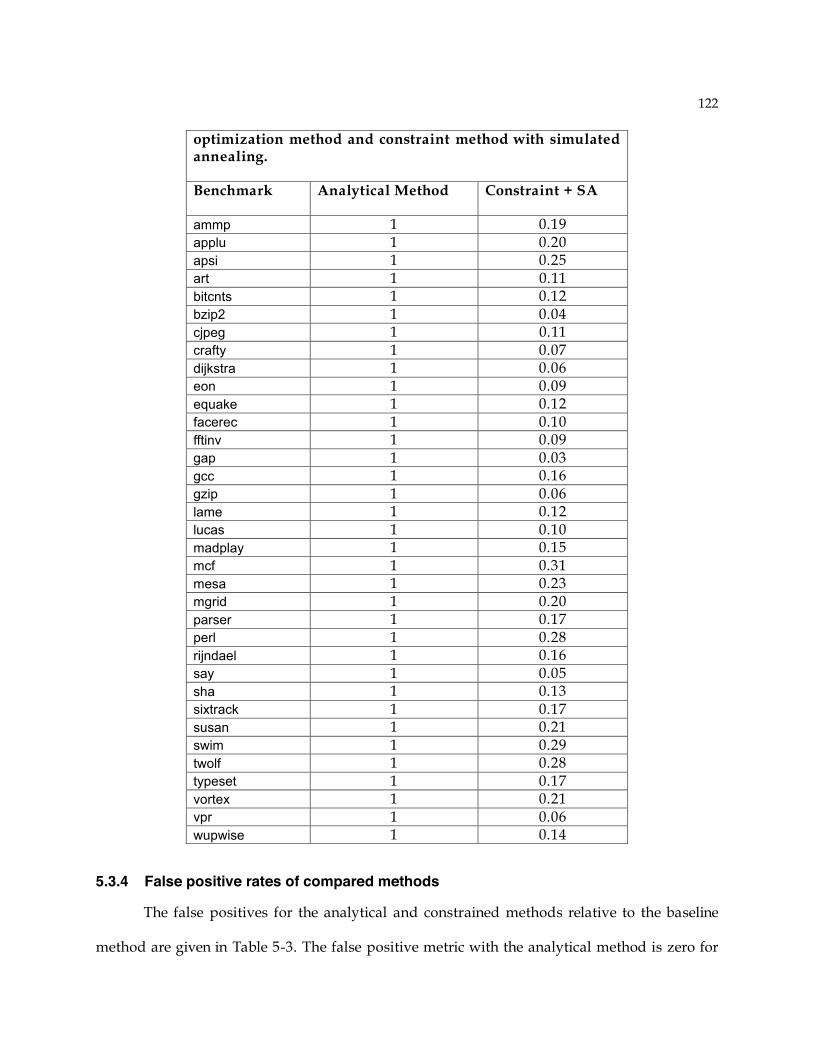
122

optimization method and constraint method with simulated annealing.

Benchmark Analytical Method Constraint + SA

ammp 1 0.19 applu 1 0.20 apsi 1 0.25 art 1 0.11 bitcnts 1 0.12 bzip2 1 0.04 cjpeg 1 0.11 crafty 1 0.07 dijkstra 1 0.06 eon 1 0.09 equake 1 0.12 facerec 1 0.10 fftinv 1 0.09 gap 1 0.03 gcc 1 0.16 gzip 1 0.06 lame 1 0.12 lucas 1 0.10 madplay 1 0.15 mcf 1 0.31 mesa 1 0.23 mgrid 1 0.20 parser 1 0.17 perl 1 0.28 rijndael 1 0.16 say 1 0.05 sha 1 0.13 sixtrack 1 0.17 susan 1 0.21 swim 1 0.29 twolf 1 0.28 typeset 1 0.17 vortex 1 0.21 vpr 1 0.06 wupwise 1 0.14

5.3.4 False positive rates of compared methods

The false positives for the analytical and constrained methods relative to the baseline

method are given in Table 5-3. The false positive metric with the analytical method is zero for

123

all benchmarks. For the assumed design space the analytical method did not classify any non-

Pareto-optimal designs as Pareto-optimal. The Simulated Annealing method, in contrast, has

a false positive metric as high as 0.39 for mcf and twolf. This is not surprising because the

heuristic algorithm of simulation annealing is known to get stuck in a local optima [15].

Table 5-3: False positive metric of the proposed method and the conventional optimization method with respect to the baseline method.

Benchmark Analytical Method Constraint + SA

ammp 0 0.19 applu 0 0.09 apsi 0 0.12 art 0 0.11 bitcnts 0 0.12 bzip2 0 0.09 cjpeg 0 0.25 crafty 0 0.16 dijkstra 0 0.10 eon 0 0.14 equake 0 0.26 facerec 0 0.22 fftinv 0 0.16 gap 0 0.09 gcc 0 0.27 gzip 0 0.09 lame 0 0.29 lucas 0 0.24 madplay 0 0.22 mcf 0 0.39 mesa 0 0.18 mgrid 0 0.14 parser 0 0.22 perl 0 0.31 rijndael 0 0.23 say 0 0.08 sha 0 0.21 sixtrack 0 0.31 susan 0 0.23 swim 0 0.27 twolf 0 0.39 typeset 0 0.27

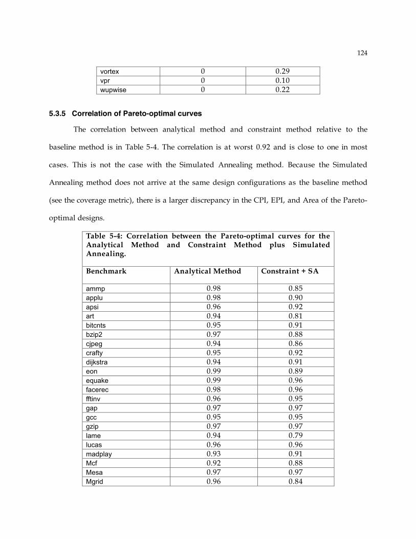
124

vortex 0 0.29 vpr 0 0.10 wupwise 0 0.22

5.3.5 Correlation of Pareto-optimal curves

The correlation between analytical method and constraint method relative to the

baseline method is in Table 5-4. The correlation is at worst 0.92 and is close to one in most

cases. This is not the case with the Simulated Annealing method. Because the Simulated

Annealing method does not arrive at the same design configurations as the baseline method

(see the coverage metric), there is a larger discrepancy in the CPI, EPI, and Area of the Pareto-

optimal designs.

Table 5-4: Correlation between the Pareto-optimal curves for the Analytical Method and Constraint Method plus Simulated Annealing.

Benchmark Analytical Method Constraint + SA

ammp 0.98 0.85 applu 0.98 0.90 apsi 0.96 0.92 art 0.94 0.81 bitcnts 0.95 0.91 bzip2 0.97 0.88 cjpeg 0.94 0.86 crafty 0.95 0.92 dijkstra 0.94 0.91 eon 0.99 0.89 equake 0.99 0.96 facerec 0.98 0.96 fftinv 0.96 0.95 gap 0.97 0.97 gcc 0.95 0.95 gzip 0.97 0.97 lame 0.94 0.79 lucas 0.96 0.96 madplay 0.93 0.91 Mcf 0.92 0.88 Mesa 0.97 0.97 Mgrid 0.96 0.84

125

parser 0.94 0.94 Perl 0.95 0.93 rijndael 0.97 0.97 Say 0.97 0.92 Sha 0.96 0.96 sixtrack 0.94 0.94 susan 0.96 0.96 Swim 0.94 0.94 Twolf 0.93 0.93 typeset 0.95 0.95 vortex 0.98 0.98 Vpr 0.98 0.98 wupwise 0.96 0.96

5.3.6 Time complexity of baseline, proposed, and conventional methods

The analytical method found Pareto-optimal designs in 16 minutes. This includes the

trace analysis to generate the function unit statistics, instruction mix, dependence statistics,

load overlap statistics, and the cache and branch predictor miss-rates. The breakdown for

optimization time of the analytical method is in Table 5-5. Most of the optimization time is

spent in trace-driven simulation of branch predictor and caches; design optimization time is

negligible.

Table 5-5: Time breakdown for processor optimization.

Task within design framework Time (sec.)

Cache miss rates 512 Branch misprediction rate 250 Instr. Dep., Func. Unit Mix, Load stats 132 Design Optimization 10

For the same design space and the same 2 GHz Pentium 4 processor it is estimated

that the baseline method would require two months to find the Pareto-optimal designs. It is

estimated that the Simulated Annealing method will arrive at the Pareto-optimal

configurations in about 24 days. The analytical method is orders of magnitude faster than

both the baseline and the Simulated Annealing methods.

126

To make evaluation of the baseline method tractable, traces of 100 million instructions

and the design space in Table 5-2 are used in this work. The embedded processor designer, in

general, can use much longer trace lengths and a larger design space. The important thing is

that the analytical method will always be orders of magnitude faster than baseline and

Simulated Annealing methods. To see why, equations are developed for design time as a

function of the number of analyzed application program instructions and the size of the design

space.

Define Gi to be the number of pre-designed components of type i in the design space,

NINSNS the number of dynamic instructions in the application software as previously denoted,

TSIM the time per instruction for detailed cycle accurate simulation, TT the time per instruction

for a cache/branch predictor trace-driven simulation, and TA the time spent for analytical

modeling of one processor configuration (Chapters 3, and 4, and Section 5.1). The design

optimization time required with the baseline method, denoted as TBM , is given by in

equation 5-9, and the design time with the analytical method denoted by TAM is given by

equation 5-10.

= ! !"BM INSNS SIM i

i

T N T G (5-9)

! "! "

= # # + #$ %$ %& ' & '

( )AM INSNS T i A i

i i

T N T G T G (5-10)

Comparing equation 5-9 to equation 5-10, one can observe that equation 5-9 for TBM

has a product term consisting of all the Gi multiplied by the detailed simulation time for the

entire application software. The same product term in equation 5-10 for TAM is multiplied only

by the time it takes to evaluate the analytical equations TA. TA is independent of the number of

instructions in the application program and will be orders of magnitude smaller than TSIM. For

127

the design space used in evaluation, TA is about 10 seconds, while cycle-accurate simulation of

one benchmark requires 45 minutes.

The portion of TAM that is a function of the benchmark length is the time required for

collecting program statistics with trace-driven simulations – (NINSNS × TT × � iGi). Because of

the independence property of the performance and energy models, and the additive property

of the area, the Gi are summed and not multiplied, thereby reducing their computation time

considerably. Furthermore, in practice TT will generally be much less than TSIM. For instance,

one trace-driven simulation TT of a branch predictor for trace length of 100 million instructions

takes about 2 minutes on a 2 GHz Pentium-4 machine, whereas a detailed cycle accurate

simulation (TSIM) of the same instructions takes 45 minutes.

Now consider the design optimization time for the Simulated Annealing method

denoted as SAT and given by the formula in equation 5-11.

(3 1)!

" #$ % %& '( )*SA i SIM INSNS

i

T G T N (5-11)

The constraint method for solving multi-objective optimization problems requires ( 1)!pr

evaluations[81], where r is the number of values EPI and Area can take, and p is the number of

objectives for which the optimization problem is evaluated. In this case, p is equal to 3,

because the design evaluation metrics are CPI, EPI, and Area. The ranges of EPI and Area

values are no less than the total number of components in the component database given as

! i

i

G .

In general the analytical method will always be faster than the Simulated Annealing

based constraint method. Comparing equation 5-11 to equation 5-10, <AM SAT T because (1) the

128

term ! "

#$ %& '

(A i

i

T G is generally small and (2) the term ! "# #$ %

& '(INSNS T i

i

N T G will always be less

than (3 1)!

" #$ $% &

' () i SIM INSNS

i

G T N .

One limitation of the analytical method is that even if it arrives at the same Pareto-

optimal designs as the baseline method, there may be a discrepancy in the CPI and EPI

estimates due to the first-order CPI and energy activity models (see Chapters 3 and 4). As a

concrete example, consider the Pareto-optimal plots of mcf in Figure 5-3 for the analytical

method and the baseline method. Figure 5-3a has the CPI versus Area plot. Notice that if the

designer sets 4.0 CPI as the constraint, the analytical method will classify the left most design

point as the point that satisfies the constraint. The baseline method on the other hand will

classify that point as an unsatisfactory point. The same is true for EPI versus Area (Figure 5-

3b) and EPI versus CPI (Figure 5-3c) Pareto-optimal curves.

mcf

Area (million rbe)

0.0 0.2 0.4 0.6 0.8 1.0 1.2 1.4 1.6

CPI

1.5

2.0

2.5

3.0

3.5

4.0

4.5

5.0

Simulation-Based Baseline Method

Analytical Model Based Method

(a)

mcf

Area (million rbe)

0.0 0.2 0.4 0.6 0.8 1.0 1.2 1.4 1.6

EPI(nJ)

20

40

60

80

100

120

140

160

Simulation-Based Baseline Method

Analytical Model Based Method

(b)

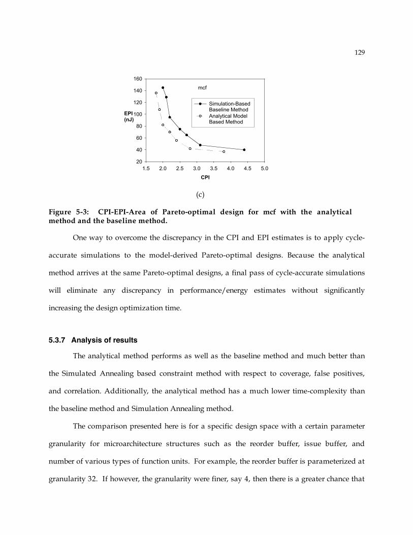
129

mcf

CPI

1.5 2.0 2.5 3.0 3.5 4.0 4.5 5.0

EPI(nJ)

20

40

60

80

100

120

140

160

Simulation-Based Baseline Method

Analytical Model Based Method

(c)

Figure 5-3: CPI-EPI-Area of Pareto-optimal design for mcf with the analytical method and the baseline method.

One way to overcome the discrepancy in the CPI and EPI estimates is to apply cycle-

accurate simulations to the model-derived Pareto-optimal designs. Because the analytical

method arrives at the same Pareto-optimal designs, a final pass of cycle-accurate simulations

will eliminate any discrepancy in performance/energy estimates without significantly

increasing the design optimization time.

5.3.7 Analysis of results

The analytical method performs as well as the baseline method and much better than

the Simulated Annealing based constraint method with respect to coverage, false positives,

and correlation. Additionally, the analytical method has a much lower time-complexity than

the baseline method and Simulation Annealing method.

The comparison presented here is for a specific design space with a certain parameter

granularity for microarchitecture structures such as the reorder buffer, issue buffer, and

number of various types of function units. For example, the reorder buffer is parameterized at

granularity 32. If however, the granularity were finer, say 4, then there is a greater chance that

130

the analytical method may select slightly different designs than the baseline method. That is, it

may have coverage less than one and false positive rate greater than one.

The advantage of the analytical method over Simulated Annealing based constraint

method is not just the higher coverage, lower false positive rate, higher correlation, and lower

time complexity. The analytical method is deterministic while the Simulated Annealing

method is not. Because of the stochastic nature of Simulated Annealing there is a variation in

the Pareto-optimal solutions, effectively yielding a “noisy” output. As a result, Simulated

Annealing has to be applied to the same problem multiple times, increasing the design

optimization time (this is not included in the reported design optimization time and the above

time-complexity equations given above).

Simulated Annealing is not the only method that yields a “noisy” output; it is a

fundamental characteristic of all black-box stochastic algorithms [84]. The analytical method

will have the same advantages over all stochastic algorithms as those demonstrated over

Simulated Annealing.

5.4 Comparison Analytical Method with Industrial Processor Implementations

The analytical method is further validated by comparing the general microarchitecture

trends provided by the analytical method to those found in implementations of commercial

superscalar processors. Two key microarchitecture trends are considered: (1) the relationship

between the Reorder Buffer and the issue width for the Pareto-optimal designs, and (2) the

relationship between Reorder Buffer and the Issue Buffer.

Issue Width and Reorder Buffer

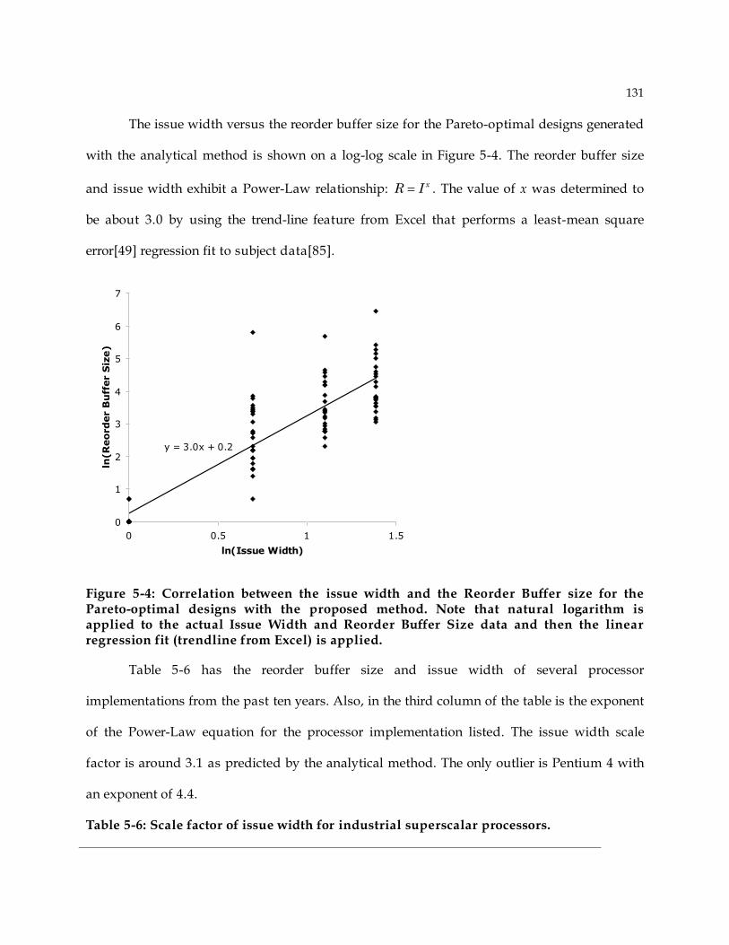
131

The issue width versus the reorder buffer size for the Pareto-optimal designs generated

with the analytical method is shown on a log-log scale in Figure 5-4. The reorder buffer size

and issue width exhibit a Power-Law relationship: xR I= . The value of x was determined to

be about 3.0 by using the trend-line feature from Excel that performs a least-mean square

error[49] regression fit to subject data[85].

y = 3.0x + 0.2

0

1

2

3

4

5

6

7

0 0.5 1 1.5

ln(Issue Width)

ln(R

eord

er B

uff

er S

ize)

Figure 5-4: Correlation between the issue width and the Reorder Buffer size for the Pareto-optimal designs with the proposed method. Note that natural logarithm is applied to the actual Issue Width and Reorder Buffer Size data and then the linear regression fit (trendline from Excel) is applied.

Table 5-6 has the reorder buffer size and issue width of several processor

implementations from the past ten years. Also, in the third column of the table is the exponent

of the Power-Law equation for the processor implementation listed. The issue width scale

factor is around 3.1 as predicted by the analytical method. The only outlier is Pentium 4 with

an exponent of 4.4.

Table 5-6: Scale factor of issue width for industrial superscalar processors.

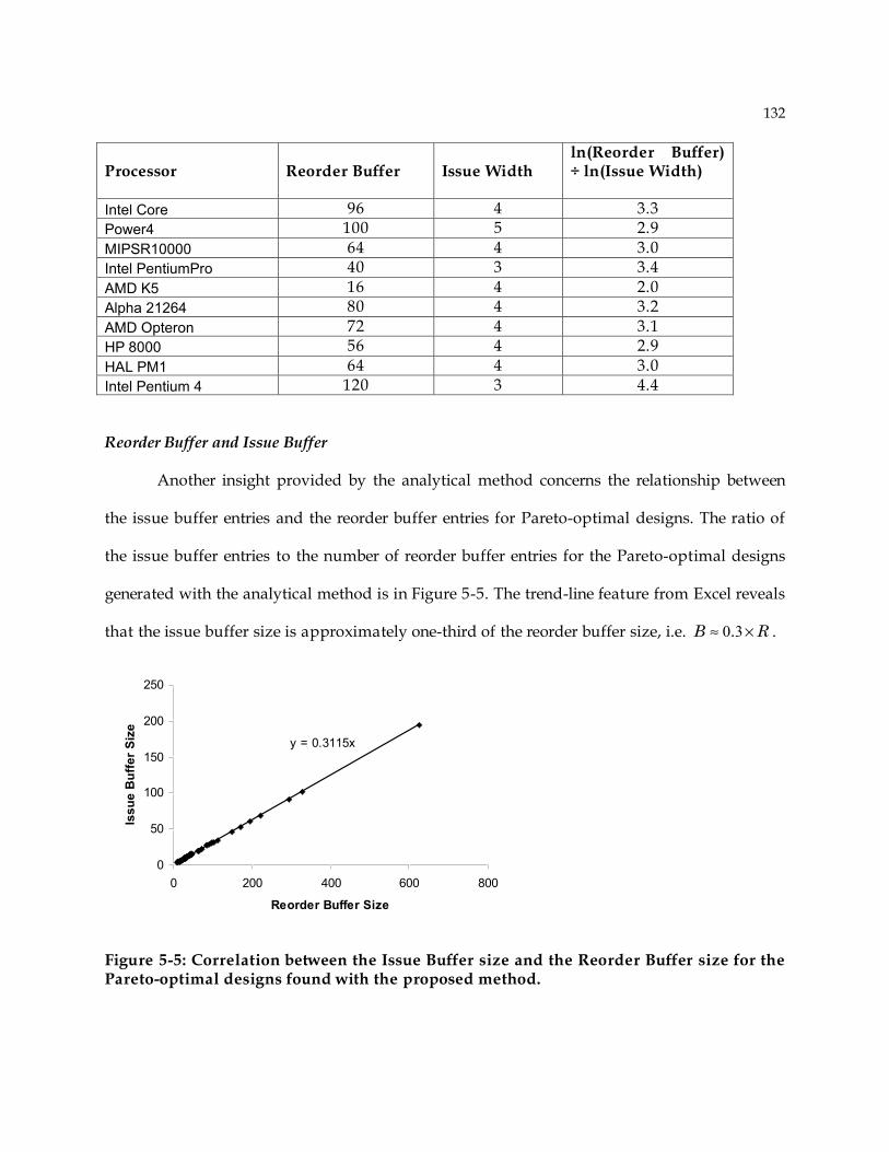
132

Processor Reorder Buffer Issue Width ln(Reorder Buffer) ÷ ln(Issue Width)

Intel Core 96 4 3.3 Power4 100 5 2.9 MIPSR10000 64 4 3.0 Intel PentiumPro 40 3 3.4 AMD K5 16 4 2.0 Alpha 21264 80 4 3.2 AMD Opteron 72 4 3.1 HP 8000 56 4 2.9 HAL PM1 64 4 3.0 Intel Pentium 4 120 3 4.4

Reorder Buffer and Issue Buffer

Another insight provided by the analytical method concerns the relationship between

the issue buffer entries and the reorder buffer entries for Pareto-optimal designs. The ratio of

the issue buffer entries to the number of reorder buffer entries for the Pareto-optimal designs

generated with the analytical method is in Figure 5-5. The trend-line feature from Excel reveals

that the issue buffer size is approximately one-third of the reorder buffer size, i.e. 0 3.B R! " .

y = 0.3115x

0

50

100

150

200

250

0 200 400 600 800

Reorder Buffer Size

Iss

ue

Bu

ffe

r S

ize

Figure 5-5: Correlation between the Issue Buffer size and the Reorder Buffer size for the Pareto-optimal designs found with the proposed method.

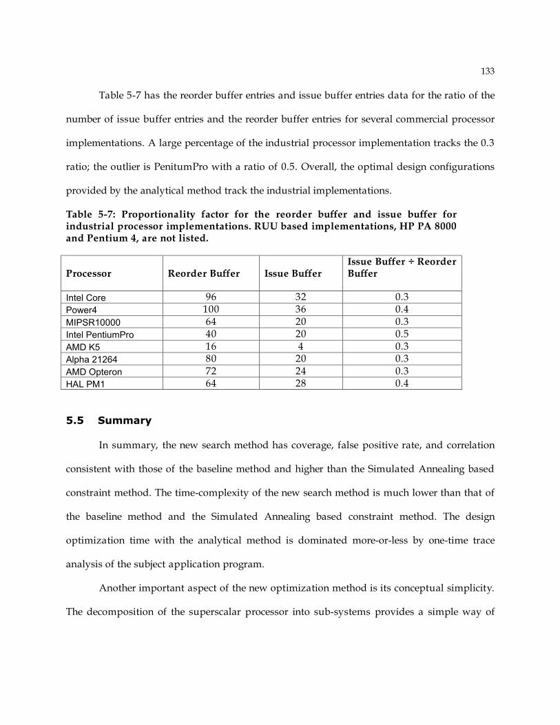
133

Table 5-7 has the reorder buffer entries and issue buffer entries data for the ratio of the

number of issue buffer entries and the reorder buffer entries for several commercial processor

implementations. A large percentage of the industrial processor implementation tracks the 0.3

ratio; the outlier is PenitumPro with a ratio of 0.5. Overall, the optimal design configurations

provided by the analytical method track the industrial implementations.

Table 5-7: Proportionality factor for the reorder buffer and issue buffer for industrial processor implementations. RUU based implementations, HP PA 8000 and Pentium 4, are not listed.

Processor Reorder Buffer Issue Buffer Issue Buffer ÷ Reorder Buffer

Intel Core 96 32 0.3 Power4 100 36 0.4 MIPSR10000 64 20 0.3 Intel PentiumPro 40 20 0.5 AMD K5 16 4 0.3 Alpha 21264 80 20 0.3 AMD Opteron 72 24 0.3 HAL PM1 64 28 0.4

5.5 Summary

In summary, the new search method has coverage, false positive rate, and correlation

consistent with those of the baseline method and higher than the Simulated Annealing based

constraint method. The time-complexity of the new search method is much lower than that of

the baseline method and the Simulated Annealing based constraint method. The design

optimization time with the analytical method is dominated more-or-less by one-time trace

analysis of the subject application program.

Another important aspect of the new optimization method is its conceptual simplicity.

The decomposition of the superscalar processor into sub-systems provides a simple way of

134

optimizing the individual sub-systems. Furthermore, the new search process provides a way to

design the superscalar processor pipeline in a systematic manner with analytical models.

135

Chapter 6: Conclusions

The competitive marketplace and the desire for high performance and functionality

place two conflicting requirements on embedded microprocessors. First, an embedded

microprocessor must often be designed with very tight time-to-market constraints. Second, the

microprocessors should be optimal in terms of performance, energy dissipation, and silicon

area for the target application(s).

The demand for functionality and high performance has led to increasing use of out-of-

order superscalar microarchitectures for high performance embedded applications. With out-

of-order superscalar processors and advances in integrate circuit technology comes the

challenge of evaluating a very large number of design options in order to find optimal

application-specific implementation(s).

System-on-chip designers choose an embedded processor and other SOC components

for designing SOCs for a particular product. Design automation of embedded processors will

allow future SOC designers to get an application-specific superscalar processor for the target

application program within the required time-to-market. One way to quickly design an

application-specific superscalar processor is to pre-design its components such as caches,

issue buffer, reorder buffer, and function units and store them in a component database along

with information about the silicon area they occupy and their energy consumption. Then a

design optimization method can find the Pareto-optimal superscalar designs after analyzing

the design options provided by the component database and target application program.

136

Unfortunately, current methods for optimizing out-of-order superscalar processors are

inadequate because they either analyze only a few designs from the design space or analyze

only a small fraction of the target application program. This dissertation contains a

computationally and conceptually simple systematic method for finding Pareto-optimal out-

of-order superscalar processors in terms of cycles-per-instruction, energy per instruction, and

silicon area. Unlike the prior design optimization methods, the method proposed here is not

limited to evaluating a small number of designs or evaluating a small fraction of an

application program.

The new design optimization method employs analytical equations that use basic

program statistics such as the instruction critical path length, function unit mix, instruction

mix, average instruction dependence chain length, and load miss overlap statistics.

Consequently, as demonstrated in Chapter 5 it is orders of magnitude faster than both a

method that uses an exhaustive search based on cycle accurate simulation and a constraint

method using Simulated Annealing.

This dissertation contributed to the development of a new CPI model, energy activity

model, and the search method. The CPI model was presented first, in Chapter 3. The CPI

model allows computation of the steady-state CPI and CPI “adders” caused by miss-events

considered in isolation (see Figure 3-1 reproduced below as Figure 6-1). The background CPI

level is determined, transient penalties due to miss-events are calculated, and these model

components are combined to arrive at accurate performance estimates. The model also

provides a method of visualizing performance losses. Branch mispredictions, instruction cache

misses, and data cache misses are analyzed by studying the phenomena that occur before and

after the miss event. This approach gives insights into individual miss-events as well as

guidance for processor optimization.

137

Figure 6-1: Useful instructions issued per cycle (IPC) as a function of clock cycles.

Next an energy activity model was developed in Chapter 4. It divides energy

dissipation into Active, Stalled, and Idle energy activities. Active energy dissipation occurs

when a component performs its intended use during a given clock cycle. Stalled energy

dissipation occurs when a component is holds useful information during a clock cycle, but

does not act on it. A component is Idle when it does not hold any useful information (or

perform any useful computation). Combinational logic and memory elements are

characterized by Active and Idle activities (Figure 4-1 and 4-2). Flip-flop based components

are described by all three activities (Figure 4-3). This method provides the insight that pipeline

stalls are a type of wasted energy activity, in addition to the wasted activities for processing

mispredicted instructions. The energy activities are related to cycles and therefore the

computation is based on the same principles as the CPI model.

The optimizing Search Method was the focus of Chapter 5. A divide-and-conquer

strategy optimizes caches, the branch predictor, and the superscalar pipeline independently.

The caches and branch predictor are optimized based on trace-driven simulation results. The

superscalar pipeline is optimized with a direct method (Figure 5-1, reproduced below as

Figure 6-2) that starts with an issue width and derives other superscalar pipeline parameters

using analytical equations.

time

IPC

branch

mispredicts

i-cache

misslong d-cache

miss

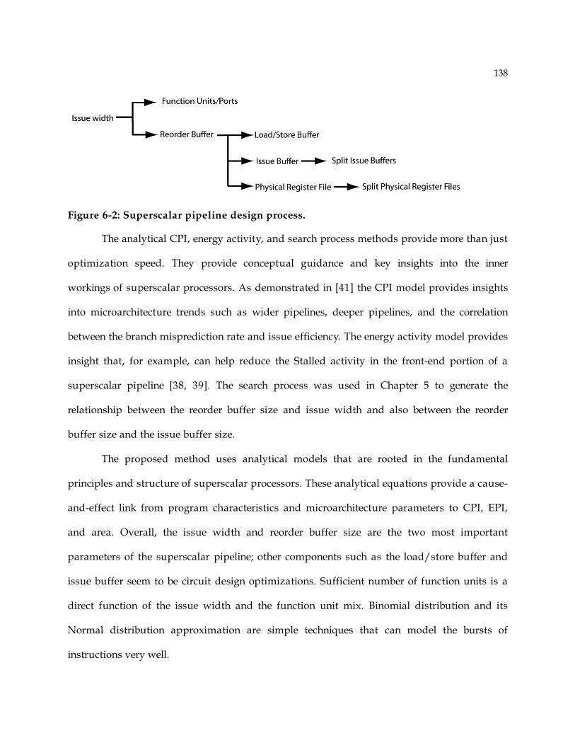
138

Figure 6-2: Superscalar pipeline design process.

The analytical CPI, energy activity, and search process methods provide more than just

optimization speed. They provide conceptual guidance and key insights into the inner

workings of superscalar processors. As demonstrated in [41] the CPI model provides insights

into microarchitecture trends such as wider pipelines, deeper pipelines, and the correlation

between the branch misprediction rate and issue efficiency. The energy activity model provides

insight that, for example, can help reduce the Stalled activity in the front-end portion of a

superscalar pipeline [38, 39]. The search process was used in Chapter 5 to generate the

relationship between the reorder buffer size and issue width and also between the reorder

buffer size and the issue buffer size.

The proposed method uses analytical models that are rooted in the fundamental

principles and structure of superscalar processors. These analytical equations provide a cause-

and-effect link from program characteristics and microarchitecture parameters to CPI, EPI,

and area. Overall, the issue width and reorder buffer size are the two most important

parameters of the superscalar pipeline; other components such as the load/store buffer and

issue buffer seem to be circuit design optimizations. Sufficient number of function units is a

direct function of the issue width and the function unit mix. Binomial distribution and its

Normal distribution approximation are simple techniques that can model the bursts of

instructions very well.

139

After the reorder buffer size is estimated, rest of the superscalar pipeline parameters

can be derived based on the reorder buffer size. The reorder buffer size is a strong function of

the average critical dependence chain length of the target program. The issue buffer size is

determined by the reorder buffer size and the average instruction dependence length. This

connection between program characteristics and superscalar processor microarchitecture

makes optimization straightforward and computationally simple.

The new design optimization method is targeted at situations where Pareto-optimal

superscalar designs are of interest with short time-to-market requirement. An embedded

processor designer, for example, may want to design a single processor that is optimal for a

set of application programs. One way to do this is generate Pareto-optimal designs for each

application program in the set of applications and then find an intersection of the Pareto-

optimal sets for each application program. If the intersected set contains one or more designs,

then one of the designs can be chosen. If the intersection set is empty, the designer will be

notified that there is no one design that will satisfy the given set of programs.

In the empty set case, the designer can pursue one of several alternatives. A straight-

forward approach is to design a single processor for a subset of the original applications.

Another option is to increase the number of components available in the component database.

The brute force method is to analyze the Pareto-optimal designs for each workload and then

choose a design that is optimal for a large fraction of the applications, where the value of the

fraction will be decided by the SOC designer. The key point is that no matter what method the

designer chooses to arrive at a single optimal processor, the analytically based optimization

method is a better alternative than the simulation based exhaustive search and stochastic

optimization algorithms such as Simulated Annealing.

140

Besides application specific processors, other areas of processor design can benefit from

the new optimization method and its individual parts. Two examples of such other areas are

given here.

Chip multiprocessor (CMP) design is one example. One way to design a CMP is with

two or more superscalar processors. Using the methods developed in this dissertation, a CMP

designer can optimize the individual superscalar processor cores. Coupled with methods that

model multiprocessor memory system, for example, the method proposed by Sorin et al. [86],

the optimal processor core to cache ratio can be derived.

Processor design in academic research is the other example. An academic researcher can

employ these methods to arrive at a well-balanced design point for their application programs.

The researcher can then investigate the benefits of a performance enhancing or energy reducing

feature on an already well-balanced superscalar processor.

6.1 Future Work

Insights presented in Chapters 3, 4, and 5 are promising methods for giving design and

cycle-accurate simulation guidance, and for ultimately reducing the time-to-market. Results

from this work also lead to additional future research.

This dissertation focused on finding Pareto-optimal superscalar processors in terms of

performance, energy, and area. Recently, temperature[87, 88] and reliability[89, 90] have

become additional design constraints. Temperature sets the thermal design point and therefore

determines the type of microprocessor packaging that is required[91, 92]. The choice of

packaging in turn determines the system cost [92]. Reliability determines the processor’s

tolerance to wear out due to soft and hard errors.

141

Methods developed in this dissertation provide the foundation for optimizing

superscalar processors in terms of performance, energy, area, temperature, and reliability. The

discrepancy in estimates for CPI loss due to branch mispredictions has already been reduced

in recent research, with the development of what is called the “Interval Analysis”[48]. Interval

Analysis explicitly accounts for the number of instructions between miss-events and then

computes the CPI and EPI significantly reducing the analytical model discrepancy than that

reported in this dissertation. The energy activity model presented in this dissertation is a basis

for developing architecture level analytical temperature and reliability models. The actual

temperature and reliability must be developed and further study is required to characterize the

accuracy, correlation, and the error of the analytical models for temperature and reliability.

142

References

[1] K. J. Nowka, G. D. Carpernter, and B. C. Brock, "The design and application of the

PowerPC 405LP energy-efficient system-on-a-chip," IBM Journal of Research and

Development, vol. 47, pp. 631-639, 2003.

[2] L. Gwennap, "MIPS R10000 Uses Decoupled Architecture," Microprocessor Report,

pp. 18-22, 1994.

[3] K. C. Yeager, "The MIPS R10000 Superscalar Microprocessor," IEEE Micro, pp. 28-

40, 1996.

[4] IBM, "PowerPC 440 Processor Core," available at http://www-306.ibm.com/.

[5] NEC, "VR5000 Series 64-bit RISC Microcomputer for multimedia applications," in

http://www.necel.com/micro/english/product/vr/vr5000series/index.html, 2006.

[6] NEC, "VR7700 Series 64-bit RISC Microcomputer for multimedia applications," in

http://www.necel.com/micro/english/product/vr/vr7700series/index.html, 2006.

[7] "Engines for Digital Age," in http://www.sandcraft.com.

[8] S. Mukherjee, et al., "Performance Simulation Tools," IEEE Computer, vol. 35, pp.

38-39, 2002.

[9] J. Krasner, "Total Cost of Development: A Comprehensive Cost Estimation

Framework for Evaluating Embedded Development Platforms," Embedded Market

Forecasters, 2003.

143

[10] S. Kirkpatrick, C. Gellat, and M. Vecchi, "Optimization by Simulated Annealing,"

Science, 1983.

[11] S. Nahar, S. Sahni, and E. Shragowitz, "Simulated Annealing and Combinatorial

Optimization," Design Automation Conference, pp. 293-299, 1986.

[12] C. C. Skiscim and B. L. Golden, "Optimization by Simulated Annealing: A

Preliminary Computational Study for the TSP," IEEE Winter Simulation

Conference, pp. 523-535, 1983.

[13] M. Locatelli, "Simulated annealing algorithms for continuous global optimization,"

in Handbook of Global Optimization II: Kluwer Academic Publishers, 2002, pp. 179-

230.

[14] B. Kumar and E. S. Davidson, "Computer System Design Using a Hierarchical

Approach to Performance Evaluation," Communications of the ACM, vol. 23, pp. 511-

521, 1980.

[15] M. A. Bhatti, Practical Optimization Methods with Mathematica Applications:

Springer Verlag, 2000.

[16] J. Kin, L. Chunho, W. H. Mangione-Smith, and M. Potkonjak, "Power efficient

mediaprocessors: design space exploration," Design Automation Conference, 1999.

Proceedings. 36th, pp. 321-326, 1999.

[17] K. Osowski and D. J. Lilja, "MinneSPEC: a new SPEC benchmark workload for

simulation-based computer architecture research," Computer Architecture Letters,

vol. 1, 2002.

[18] L. Eeckhout, H. Vandierendonck, and K. De Bosschere, "Designing computer

architecture research workloads," Computer, vol. 36, pp. 65-71, 2003.

144

[19] J. J. Yi, S. V. Kodakara, R. Sendag, D. J. Lilja, and D. M. Hawkins, "Characterizing

and comparing prevailing simulation techniques," High-Performance Computer

Architecture, 2005. HPCA-11. 11th International Symposium on, pp. 266-277, 2005.

[20] T. M. Conte, "Systematic Computer Architecture Prototyping," PhD Thesis:

University of Illinois, 1992.

[21] T. Sherwood, E. Perelman, G. Hamerly, and B. Calder, "Automatically

Characterizing Large Scale Program Behavior," presented at ASPLOS, San Jose,

CA, 2002.

[22] P. Erez, H. Greg, B. Michael Van, S. Timothy, and C. Brad, "Using SimPoint for

accurate and efficient simulation," in Proceedings of the 2003 ACM SIGMETRICS

international conference on Measurement and modeling of computer systems. San

Diego, CA, USA: ACM Press, 2003.

[23] R. E. Wunderlich, T. F. Wenisch, B. Falsafi, and J. C. Hoe, "SMARTS: accelerating

microarchitecture simulation via rigorous statistical sampling," in International

Symposium on Computer Architecture, 2003, pp. 84-97.

[24] B. A. Fields, R. Bodik, M. Hill, D., and C. J. Newburn, "Interaction cost and shotgun

profiling," ACM Trans. Archit. Code Optim., vol. 1, pp. 272-304, 2004.

[25] B. A. Fields, R. Bodik, and M. Hill, D., "Slack: maximizing performance under

technological constraints," in Proceedings of the 29th annual international

symposium on Computer architecture. Anchorage, Alaska: IEEE Computer Society,

2002.

[26] B. A. Fields, S. Rubin, and R. Bodik, "Focusing processor policies via critical-path

prediction," in Proceedings of the 28th annual international symposium on Computer

architecture. G\&\#246;teborg, Sweden: ACM Press, 2001.

145

[27] S. Nussbaum and J. E. Smith, "Modeling Superscalar Processors via Statistical

Simulation," in Parallel Architectures and Compilation Techniques, 2001, pp. 15-24.

[28] L. Eeckhout, "Accurate Statistical Workload Modeling." Gent, Belgium: University

Of Gent, 2002.

[29] M. Oskin, F. T. Chong, and M. Farrens, "HLS: combining statistical and symbolic

simulation to guide microprocessor designs," in International symposium on

Computer architecture, 2000, pp. 71-82.

[30] S. Eyerman, L. Eeckhout, and K. De Bosschere, "Efficient Design Space Exploration

of High Performance Embedded Out-of-Order Processors," in Design and Test in

Europe (DATE), 2006.

[31] E. Riseman and C. Foster, "The Inhibition of Potential Parallelism by Conditional

Jumps," IEEE Trans. on Computer Architectures, vol. C-21, pp. 1405-1411, 1972.

[32] P. Michaud, A. Seznec, and S. Jourdan, "An Exploration of Instruction Fetch

Requirement in Out-Of-Order Superscalar Processors," International Journal of

Parallel Processing, vol. 29, 2001.

[33] P. Michaud, A. Seznec, and S. Jourdan, "Exploring Instruction-Fetch Bandwidth

Requirement in Wide-Issue Superscalar Processors," presented at PACT, Newport

Beach, USA, 1999.

[34] A. Hartstein and R. P. Thomas, "The optimum pipeline depth for a microprocessor,"

in Proceedings of the 29th annual international symposium on Computer

architecture. Anchorage, Alaska: IEEE Computer Society, 2002.

[35] A. Hartstein and R. P. Thomas, "Optimum Power/Performance Pipeline Depth," in

Proceedings of the 36th annual IEEE/ACM International Symposium on

Microarchitecture: IEEE Computer Society, 2003.

146

[36] D. B. Noonburg and J. P. Shen, "Theoretical Modeling of Superscalar Processor

Performance," in International Symposium on Microarchitecture, 1994, pp. 52-62.

[37] T. Sherwood, S. Sair, and B. Calder, "Phase Tracking and Prediction," presented at

ISCA, San Diego, CA, 2003.

[38] T. Karkhanis, J. E. Smith, and P. Bose, "Saving Energy with Just-In-Time

Instruction Delivery," presented at International Symposium on Low Power

Electronics and Design, Monterey, CA, 2002.

[39] A. Buyuktosunoglu, T. Karkhanis, D. H. Albonesi, and P. Bose, "Energy Efficient Co-

Adaptive Instruction Fetch and Issue," International Symposium on Computer

Architecture, pp. 147-156, 2003.

[40] T. Taha and D. S. Wills, "An Instruction Throughput Model of Superscalar

Processors," International Workshop on Rapid Systems Prototyping, pp. 156-163,

2003.

[41] T. Karkhanis and J. E. Smith, "A Firsr-Order Superscalar Processor Model," in

International Symposium on Computer Architecture, 2004, pp. 338-349.

[42] T. Karkhanis and J. E. Smith, "A Day in the Life of a Data Cache Miss," Workshop

on Memory Performance Issues, 2002.

[43] E. D. Lazowska, J. Zahojan, G. S. Graham, and K. C. Sevcik, Quantitative System

Performance: Prentice Hall, 1984.

[44] J. M. Tendler, et. al., "IBM Power 4: System Microarchitecture," IBM Journal of

Research and Development, pp. 5-26, 2002.

[45] C. J. Anderson, et. al., "Physcial Design of a Fourth-Generation POWER GHz

Microprocessor," International Solid-State Circuits Conference, 2001.

147

[46] N. P. Jouppi, "The Nonuniform Distribution of Instruction-Level and Machine

Parallelism and Its Effect on Performance," IEEE Trans. on Computers, vol. 38, pp.

1645-1658, 1989.

[47] T. M. Conte, K. N. Menezes, P. M. Mills, and B. A. Patel, "Optimization of

Instruction Fetch Mechanisms for High Issue Rates," in International Symposium on

Computer Architecture, 1995.

[48] S. Eyerman, J. E. Smith, and L. Eeckhout, "Characterizing the branch misprediction

penalty," in International Symposium on Performance Analysis of Systems and

Software, 2006, pp. 48-58.

[49] S. Kachigan, Statistical Analysis. New York: Radius Press, 1986.

[50] "NIST/SEMATECH e-Handbook of Statistical Methods," vol. 2006:

http://www.itl.nist.gov/div898/handbook/.

[51] M. Nemani and F. N. Najm, "High-level area and power estimation for VLSI

circuits," Computer-Aided Design of Integrated Circuits and Systems, IEEE

Transactions on, vol. 18, pp. 697-713, 1999.

[52] J. N. Kozhaya and F. N. Najm, "Accurate power estimation for large sequential

circuits," Computer-Aided Design, 1997. Digest of Technical Papers., 1997

IEEE/ACM International Conference on, pp. 488-493, 1997.

[53] S. Gupta and F. N. Najm, "Energy and peak-current per-cycle estimation at RTL,"

Very Large Scale Integration (VLSI) Systems, IEEE Transactions on, vol. 11, pp.

525-537, 2003.

[54] "Star-Hspice Manual," Release 2001.2, June 2001.

[55] L. Jiing-Yuan, L. Tai-Chien, and S. Wen-Zen, "A Cell-based Power Estimation In

Cmos Combinational Circuits," 1994.

148

[56] L. Jiing-Yuan, S. Wen-Zen, and J. Jing-Yang, "A power modeling and

characterization method for the CMOS standard cell library," 1996.

[57] V. Zyuban and P. Kogge, "Application of STD to latch-power estimation," Very Large

Scale Integration (VLSI) Systems, IEEE Transactions on, vol. 7, pp. 111-115, 1999.

[58] F. N. Najm, "A survey of power estimation techniques in VLSI circuits," Very Large

Scale Integration (VLSI) Systems, IEEE Transactions on, vol. 2, pp. 446-455, 1994.

[59] D. Brooks, V. Tiwari, and M. Martonosi, "Wattch: a framework for architectural-

level power analysis and optimizations," in International Symposium on Computer

Architecture, 2000, pp. 83-94.

[60] P. Bose, et. al., "Early-Stage Definition of LPX: A Low Power Issue-Execute

Processor," Lecture Notes in Computer Science, vol. 2325, pp. 1-17, 2003.

[61] V. Kursun and E. G. friedman, "Sleep Switch Dual Threshold Voltage Domino Logic

with Reduced Standby Leakage Current," IEEETransactions on Very Large Scale

Integration Systems, vol. 12, pp. 485-496, 2004.

[62] R. E. Kessler, "The Alpha 21264 microprocessor," IEEE Micro, vol. 19, pp. 24-36,

1999.

[63] J. L. Miller, J. Conary, and D. DiMarco, "A 16 GB/s, 0.18 &mu;m cache tile for

integrated L2 caches from 256," 2000.

[64] D. H. Wolpert and W. G. MacReady, "The Mathematics of Search," 1996.

[65] S. Przybylski, M. Horowitz, and J. Hennessy, "Characteristics Of Performance-

Optimal Multi-level Cache Hierarchies," 1989.

[66] X. Vera, N. Bermudo, J. Llosa, and A. Gonzalez, "A fast and accurate framework to

analyze and optimize cache memory behavior," ACM Trans. Program. Lang. Syst.,

vol. 26, pp. 263-300, 2004.

149

[67] E. Berg and E. Hagersten, "StatCache: A Probabilistic Approach to Efficient and

Accurate Data Locality Analysis," International Symposium on Performance

Analysis of Systems and Software, 2004.

[68] B. B. Fraguela, R. Doallo, and E. L. Zapata, "Automatic analytical modeling for the

estimation of cache misses," 1999.

[69] J. Xue and X. Vera, "Efficient and accurate analytical modeling of whole-program

data cache behavior," Computers, IEEE Transactions on, vol. 53, pp. 547-566, 2004.

[70] A. Agarwal, J. Hennessy, and M. Horowitz, "An analytical cache model," ACM

Trans. Comput. Syst., vol. 7, pp. 184-215, 1989.

[71] S. H. John, J. K. Darren, and R. N. Graham, "Analytical Modeling of Set-Associative

Cache Behavior," IEEE Trans. Comput., vol. 48, pp. 1009-1024, 1999.

[72] G. E. Suh, D. Srinivas, and R. Larry, "Analytical cache models with applications to

cache partitioning," in Proceedings of the 15th international conference on

Supercomputing. Sorrento, Italy: ACM Press, 2001.

[73] M. D. Hill, J. R. Larus, A. R. Lebeck, M. Talluri, and D. A. Wood, "Wisconsin

Architectural Research Tool Set," Computer Architecture News, vol. 21, pp. 8-10,

1993.

[74] M. D. Hill and A. J. Smith, "Evaluating Asociativity in CPU Caches," IEEE

Transactions on Computers, 1989.

[75] N. P. Jouppi and D. W. Wall, "Available Instruction-Level Parallelism for

Superscalar and Superpipelined Machines," presented at Architectural Support for

Programming Languages and Operating Systems, Boston, MA, 1989.

150

[76] K. B. Theobald, G. R. Gao, and L. J. Hendren, "On the Limits of Program

Parallelism and its Smoothability," International Symposium on Microarchitecture,

pp. 10-19, 1992.

[77] S. Ross, A First Course in Probability: Prentice Hall, 2005.

[78] G. Hinton, D. Sager, M. Upton, D. Boggs, D. Carmean, A. Kyker, and P. Roussel,

"The Microarchitecture of the Pentium 4 Processor," Intel Technology Journal, vol.

Q1, 2001.

[79] L. Gwennap, "Intel's P6 Uses Decoupled Superscalar Design," Microprocessor

Report, vol. 9, 1995.

[80] Y. Sawaragi, H. Nakayama, and T. Tamino, Theory of Multiobjective Optimization:

Orland Academic Press, 1985.

[81] J. L. Cohon, Multiobjective Programming and Planning. Mineola, New York: Dover

Publications, INC, 2003.

[82] J. M. Mulder and M. Flynn, "An Area Model for On-Chip Memories and its

Application," IEEE Journal of Solid-State Circuits, vol. 26, pp. 98-106, 1991.

[83] M. J. Flynn, Computer Architecture: Pipelined and Parallel Processor Design: Jones

and Bartlett Publishers, 1995.

[84] Z. Michalewicz and D. B. Fogel, How to Solve it: Modern Heuristics. New York:

Springer-Verlag, 2000.

[85] W. L. Winston, Microsoft Excel Data Analysis and Business Modeling: Microsoft

Press, 2004.

[86] D. J. Sorin, V. S. Pai, S. V. Adve, M. K. Vernon, and D. A. Wood, "Analytic

Evaluation of Shared-Memory Systems with ILP Processors," in International

Symposium on Computer Architecture: IEEE Computer Society, 1998, pp. 380-391.

151

[87] K. Skadron, K. Sankaranarayanan, S. Velusamy, D. Tarjan, M. R. Stan, and W.

Huang, "Temperature-Aware Microarchitecture: Modeling and Implementation,"

ACM Transactions on Architecture and Code Optimization, vol. 1, pp. 94-125, 2004.

[88] K. Skadron, M. R. Stan, W. Huang, S. Velusamy, K. Sankaranarayanan, and D.

Tarjan, "Temperature-Aware Microarchitecture," in International Symposium on

Computer Architecture: ACM Press, 2003, pp. 2-13.

[89] S. Mukherjee, J. Emer, and S. K. Reinhardt, "The Soft Error Problem: An

Architectural Perspective," in International Symposium on High Performance

Computer Architecture, 2005.

[90] J. Srinivasan, S. Adve, P. Bose, and J. Rivers, "The Case for Lifetime Reliability-

Aware Microprocessors," in International Symposium on Computer Architecture,

2004.

[91] R. Mahajan, K. Brown, and V. Atluri, "The Evolution of Microprocessor Packaging,"

Intel Technology Journal, vol. Q3, 2000.

[92] J. Lau, Ball Grid Array Technology: McGraw-Hill Professional, 1994.