Embed Size (px)
Citation preview
Autonomous Navigation for
Airborne Applications
Jonghyuk Kim
A thesis submitted in fulfillment
of the requirements for the degree of
Doctor of Philosophy
Australian Centre for Field Robotics
Department of Aerospace, Mechanical and Mechatronic Engineering
The University of Sydney
May 2004

Declaration
I hereby declare that this submission is my own work and that, to the best of my
knowledge and belief, it contains no material previously published or written by
another person nor material which to a substantial extent has been accepted for the
award of any other degree or diploma of the University or other institute of higher
learning, except where due acknowledgement has been made in the text.
Jonghyuk Kim
May 1, 2004
i
ii
Abstract
Jonghyuk Kim Doctor of PhilosophyThe University of Sydney May 2004
Autonomous Navigation forAirborne Applications
Autonomous navigation (or localisation) is the process of determining a platform’spose without the use of any a priori information external to the platform except forwhat the platform senses about the environment. That is, the determination of theplatform’s pose without the use of predefined maps or infrastructure developed fornavigation purposes such as terrain aided navigation systems or Global NavigationSatellite System (GNSS). The objective of this thesis is to both develop and demon-strate autonomous localisation algorithms for airborne platforms. The emphasis isplaced on the importance of the algorithms to function appropriately and accuratelyusing low cost inertial sensors (where the rapid drift in navigation output requiresan increasing reliance on frequent absolute sensing), within an environment wherethe highly dynamic nature of the platform motion provides unreliable and infrequentabsolute sensing. There are five main contributions to this thesis:
Firstly, is the theoretical formulation of the autonomous localisation algorithmfor a 6DoF (Degree of Freedom) platform. The process takes on the form of theSimultaneous Localisation and Mapping (SLAM) algorithm which has been quiteextensively formulated for the indoor robotics community and for outdoor land vehicleapplications. In all these applications though only a 2D problem is posed simplifyingthe task significantly. By formulating the problem within a 6DoF framework, theSLAM algorithm is now opened to any platform description. In order to developsuch a generic model, no absolute platform model can be implemented (which isadvantageous) and hence the use of inertial navigation techniques are required inorder to allow for prediction of state information, which is developed within thisthesis.
Secondly, is the recasting of the SLAM algorithm in order to improve its compu-tational efficiency. SLAM is an expensive process, and more so when the frameworkcalls for 6DoF implementation. Moreover, increasing the number of states which arerequired to be estimated such as inertial sensor errors, and having the fundamentalrequirement of high sampling rates when using inertial sensors, further exacerbatesthe problem. To overcome this the algorithm is casted into its error form which
iii
models the error propagation in SLAM, that is, the error propagation of the statesand the map. Since, in most cases, the dynamics of the error propagation is signifi-cantly slower than the dynamics of the platform itself, then dramatic improvementsin computational efficiency take place.
Thirdly, the thesis will add to the already significant research activity in thedevelopment of multi-vehicle SLAM, where platforms share map information in orderto both improve the quality and the localisation of the platforms. The main focus isnot the development of a new algorithm, but the actual implementation of the 6DoFframework within this context.
Fourthly, in order to validate the effectiveness of SLAM, the real-time implemen-tation of the algorithm is developed for a highly dynamic Uninhabited Air Vehicle(UAV). The purpose is to provide a significant engineering contribution towards theknowledge of implementation. The results of the real-time algorithm is compared toan GNSS/Inertial navigation system, to illustrate the validity of the output.
Finally, this thesis also presents a reliable GNSS/Inertial navigation system whichcouples information from a barometric altimeter. Although not a primary goal (thedevelopment was only required to provide a tool to validate the SLAM output), it wasfound that within highly dynamic environments, low-cost GNSS sensors are vulnera-ble to outages and long satellite reacquisition times, and hence the INS requires extraaiding, predominately in the form of height information. Furthermore, the real-timeimplementation of the GNSS/Inertial navigation system is also presented, forminganother main engineering contribution to this thesis.
Acknowledgements
I would like to thank my supervisor Dr Salah Sukkarieh for his support, guidance,optimism and enthusiasm throughout the past four years. Salah was always availableto give help whenever it was needed. I would also like to thank Professor EduardoNebot and Professor Hugh Durrant-Whyte for their support and help during thisresearch.
I must give special thanks to all the members of the ANSER project: StuartWishart for building the avionic systems and gluing the whole system to make itwork together, Jeremy Randle for building and flying the UAVs, Matt Ridley forbuilding the vision system, Ali Goktogan for his effort with the communication andradar system, Eric Nettleton for building the decentralised system, Alan Trinder forlaughs and the fake snake in Marulan, Gurce Isikyildiz and Chris Mifsud for thehardware and software they designed. Thanks also to the staff at BAE Systems fortheir help: Julia, Owen and Paul for the advices and discussions to improve thesystem. We spent lots of days and nights on the test sites to make the system work,and finally watching the working system was the most exciting moment being here.
To all the other members of the ACFR group, I owe a special thanks to JoseGuivant for his invaluable helps and discussions during the period. To Juan Nieto,for his help demonstrating the GINTIC project. To Ross Hennessy for the beautifulfish tank next to my desk. To Alex and Fred for the night climbing of Mt. Fuji inJapan. To Gerold, Tim, Richard, Ralph, Trevor, Mark, Andrew, Tomo, Mari, Shron,Fabio, Mitch and Ben for their help and sense of humour, and all the others who havevisited and gone from ACFR. I would particularly like to thank Anna for her help inACFR. Thanks to Simon Lacroix, Allonzo Kelly and Stefan Williams for the reviewsof my thesis and invaluable advices.
Thanks to my family for their loves and concerns. To Charles and Ruby, youbrought me the joy and happiness of the life. Finally a special thank to Hyeja, foryour love and understanding.
iv

To Charles, Ruby and Hyeja
Contents
Declaration i
Abstract ii
Acknowledgements iv
Contents vi
List of Abbreviations xii
List of Figures xiii
List of Tables xxiii
1 Introduction 1
1.1 Airborne Simultaneous Localisation and Mapping . . . . . . . . . . . 3
1.2 GNSS Aided Airborne Navigation . . . . . . . . . . . . . . . . . . . . 7
1.3 Contributions . . . . . . . . . . . . . . . . . . . . . . . . . . . . . . . 7
1.4 Thesis Structure . . . . . . . . . . . . . . . . . . . . . . . . . . . . . . 9
2 Statistical estimation 12
2.1 Introduction . . . . . . . . . . . . . . . . . . . . . . . . . . . . . . . . 12
2.2 Bayesian Estimation . . . . . . . . . . . . . . . . . . . . . . . . . . . 12
2.3 Kalman Filter . . . . . . . . . . . . . . . . . . . . . . . . . . . . . . . 15
2.4 Extended Kalman Filter . . . . . . . . . . . . . . . . . . . . . . . . . 19
vi
CONTENTS vii
2.5 Information Filter . . . . . . . . . . . . . . . . . . . . . . . . . . . . . 22
2.6 Extended Information Filter . . . . . . . . . . . . . . . . . . . . . . . 25
2.7 Filter Configurations for Aided Inertial Navigation . . . . . . . . . . . 26
2.7.1 Advantages and Disadvantages of the Direct and Indirect filterStructures . . . . . . . . . . . . . . . . . . . . . . . . . . . . . 28
2.7.2 6DoF SLAM Structure . . . . . . . . . . . . . . . . . . . . . . 29
2.7.3 GNSS/Inertial Navigation Structure . . . . . . . . . . . . . . 31
2.7.4 GNSS/Inertial/Baro Navigation Structure . . . . . . . . . . . 31
2.8 Summary . . . . . . . . . . . . . . . . . . . . . . . . . . . . . . . . . 33
3 Strapdown Inertial Navigation 34
3.1 Introduction . . . . . . . . . . . . . . . . . . . . . . . . . . . . . . . . 34
3.2 Inertial Measurement Unit (IMU) . . . . . . . . . . . . . . . . . . . . 35
3.3 Coordinate Systems . . . . . . . . . . . . . . . . . . . . . . . . . . . . 36
3.3.1 Inertial Frame . . . . . . . . . . . . . . . . . . . . . . . . . . . 37
3.3.2 Earth-Centred Earth-Fixed Frame . . . . . . . . . . . . . . . . 37
3.3.3 Geographic Frame . . . . . . . . . . . . . . . . . . . . . . . . 38
3.3.4 Earth-Fixed Local-Tangent Frame . . . . . . . . . . . . . . . . 38
3.3.5 Body Frame . . . . . . . . . . . . . . . . . . . . . . . . . . . . 39
3.3.6 Sensor Frame . . . . . . . . . . . . . . . . . . . . . . . . . . . 39
3.4 Inertial Navigation Equations . . . . . . . . . . . . . . . . . . . . . . 40
3.4.1 Attitude Equations . . . . . . . . . . . . . . . . . . . . . . . . 40
3.4.2 Velocity/Position Equations . . . . . . . . . . . . . . . . . . . 50
3.5 Error Analysis . . . . . . . . . . . . . . . . . . . . . . . . . . . . . . . 54
3.5.1 Attitude Error Equations . . . . . . . . . . . . . . . . . . . . . 54
3.5.2 Velocity/Position Error Equations . . . . . . . . . . . . . . . . 56
3.6 IMU Lever-arm . . . . . . . . . . . . . . . . . . . . . . . . . . . . . . 59
3.7 Vibration . . . . . . . . . . . . . . . . . . . . . . . . . . . . . . . . . 60
3.7.1 Sampling Frequency . . . . . . . . . . . . . . . . . . . . . . . 60
3.7.2 Coning Error . . . . . . . . . . . . . . . . . . . . . . . . . . . 62
3.8 Initial Calibration and Alignment . . . . . . . . . . . . . . . . . . . . 65
3.9 Summary . . . . . . . . . . . . . . . . . . . . . . . . . . . . . . . . . 66
CONTENTS viii
4 Airborne 6DoF SLAM Navigation 67
4.1 Introduction . . . . . . . . . . . . . . . . . . . . . . . . . . . . . . . . 67
4.2 6DoF SLAM Algorithm . . . . . . . . . . . . . . . . . . . . . . . . . 68
4.2.1 Augmented State . . . . . . . . . . . . . . . . . . . . . . . . . 69
4.2.2 Nonlinear Process Model . . . . . . . . . . . . . . . . . . . . . 70
4.2.3 Relationship between Observation and Landmarks . . . . . . . 74
4.2.4 Nonlinear Observation Model . . . . . . . . . . . . . . . . . . 76
4.2.5 Prediction . . . . . . . . . . . . . . . . . . . . . . . . . . . . . 79
4.2.6 Estimation . . . . . . . . . . . . . . . . . . . . . . . . . . . . . 79
4.2.7 Data Association . . . . . . . . . . . . . . . . . . . . . . . . . 80
4.2.8 New Landmark Augmentation . . . . . . . . . . . . . . . . . . 81
4.2.9 Error Analysis on the Initialised Landmarks . . . . . . . . . . 83
4.3 Indirect 6DoF SLAM Algorithm . . . . . . . . . . . . . . . . . . . . . 85
4.3.1 External Inertial Navigation Loop . . . . . . . . . . . . . . . . 87
4.3.2 External Map . . . . . . . . . . . . . . . . . . . . . . . . . . . 87
4.3.3 Augmented Error State . . . . . . . . . . . . . . . . . . . . . . 88
4.3.4 Error Process Model . . . . . . . . . . . . . . . . . . . . . . . 88
4.3.5 Error Observation Model . . . . . . . . . . . . . . . . . . . . . 91
4.3.6 Prediction . . . . . . . . . . . . . . . . . . . . . . . . . . . . . 92
4.3.7 Estimation . . . . . . . . . . . . . . . . . . . . . . . . . . . . . 92
4.3.8 Data Association and New Landmark Initialisation . . . . . . 93
4.3.9 Feedback Error Correction . . . . . . . . . . . . . . . . . . . . 94
4.4 DDF 6DoF SLAM . . . . . . . . . . . . . . . . . . . . . . . . . . . . 95
4.5 Summary . . . . . . . . . . . . . . . . . . . . . . . . . . . . . . . . . 100
5 GNSS/Inertial Airborne Navigation 102
5.1 Introduction . . . . . . . . . . . . . . . . . . . . . . . . . . . . . . . . 102
5.2 GNSS Overview . . . . . . . . . . . . . . . . . . . . . . . . . . . . . . 103
5.3 GNSS/Inertial Integration . . . . . . . . . . . . . . . . . . . . . . . . 104
CONTENTS ix
5.3.1 Process Model . . . . . . . . . . . . . . . . . . . . . . . . . . . 106
5.3.2 Observation Model . . . . . . . . . . . . . . . . . . . . . . . . 108
5.3.3 Prediction . . . . . . . . . . . . . . . . . . . . . . . . . . . . . 109
5.3.4 Estimation . . . . . . . . . . . . . . . . . . . . . . . . . . . . . 109
5.3.5 Feedback Error Correction . . . . . . . . . . . . . . . . . . . . 110
5.4 Observation Matching . . . . . . . . . . . . . . . . . . . . . . . . . . 111
5.4.1 Observation Latency . . . . . . . . . . . . . . . . . . . . . . . 111
5.4.2 GNSS Lever-arm . . . . . . . . . . . . . . . . . . . . . . . . . 114
5.4.3 GNSS Lever-arm Error Analysis . . . . . . . . . . . . . . . . . 114
5.5 Baro-altimeter Augmented GNSS/Inertial Navigation . . . . . . . . . 118
5.5.1 Baro-altimeter Error Model . . . . . . . . . . . . . . . . . . . 123
5.5.2 Process Model . . . . . . . . . . . . . . . . . . . . . . . . . . . 124
5.5.3 Observation Model . . . . . . . . . . . . . . . . . . . . . . . . 124
5.6 Summary . . . . . . . . . . . . . . . . . . . . . . . . . . . . . . . . . 125
6 Real-time Implementation 126
6.1 Introduction . . . . . . . . . . . . . . . . . . . . . . . . . . . . . . . . 126
6.2 The ANSER Project . . . . . . . . . . . . . . . . . . . . . . . . . . . 126
6.3 Flight Vehicle . . . . . . . . . . . . . . . . . . . . . . . . . . . . . . . 127
6.4 Sensors . . . . . . . . . . . . . . . . . . . . . . . . . . . . . . . . . . . 129
6.4.1 IMU . . . . . . . . . . . . . . . . . . . . . . . . . . . . . . . . 130
6.4.2 GPS . . . . . . . . . . . . . . . . . . . . . . . . . . . . . . . . 131
6.4.3 Baro-altimeter . . . . . . . . . . . . . . . . . . . . . . . . . . . 133
6.4.4 Inclinometer . . . . . . . . . . . . . . . . . . . . . . . . . . . . 134
6.4.5 Vision System . . . . . . . . . . . . . . . . . . . . . . . . . . . 134
6.4.6 Vision/Laser System . . . . . . . . . . . . . . . . . . . . . . . 137
6.4.7 Radar System . . . . . . . . . . . . . . . . . . . . . . . . . . . 137
6.5 GNSS/Inertial Navigation System . . . . . . . . . . . . . . . . . . . . 139
6.5.1 Hardware Development . . . . . . . . . . . . . . . . . . . . . . 139

CONTENTS x
6.5.2 Software Development . . . . . . . . . . . . . . . . . . . . . . 143
6.6 Airborne 6DoF SLAM System . . . . . . . . . . . . . . . . . . . . . . 150
6.6.1 Hardware Development . . . . . . . . . . . . . . . . . . . . . . 150
6.6.2 Software Development . . . . . . . . . . . . . . . . . . . . . . 150
6.7 Hardware-In-The-Loop (HWIL) System . . . . . . . . . . . . . . . . . 151
6.8 Summary . . . . . . . . . . . . . . . . . . . . . . . . . . . . . . . . . 153
7 Experimental Results 154
7.1 Introduction . . . . . . . . . . . . . . . . . . . . . . . . . . . . . . . . 154
7.2 Flight Test Setup . . . . . . . . . . . . . . . . . . . . . . . . . . . . . 155
7.3 Real-time GNSS/Inertial Navigation Results . . . . . . . . . . . . . . 155
7.4 Baro-augmented GNSS/Inertial Navigation Results . . . . . . . . . . 160
7.5 Post-processed 6DoF SLAM results . . . . . . . . . . . . . . . . . . . 162
7.6 Real-time 6DoF SLAM Results . . . . . . . . . . . . . . . . . . . . . 163
7.7 Summary . . . . . . . . . . . . . . . . . . . . . . . . . . . . . . . . . 166
7.8 Plots of GNSS/Inertial Navigation Results . . . . . . . . . . . . . . . 167
7.9 Plots of GNSS/Inertial/Baro Navigation Results . . . . . . . . . . . . 176
7.10 Plots of Post-processed 6DoF SLAM . . . . . . . . . . . . . . . . . . 179
7.11 Plots of Real-time 6DoF SLAM . . . . . . . . . . . . . . . . . . . . . 184
8 Further Analysis on Airborne SLAM 191
8.1 Introduction . . . . . . . . . . . . . . . . . . . . . . . . . . . . . . . . 191
8.2 Analysis of Varying Sensor Characteristics on SLAM . . . . . . . . . 192
8.2.1 A Comparison Between the Vision and Radar Sensors . . . . . 195
8.3 A Comparison of Direct and Indirect SLAM . . . . . . . . . . . . . . 196
8.4 Observability of SLAM . . . . . . . . . . . . . . . . . . . . . . . . . . 197
8.5 DDF 6DoF SLAM . . . . . . . . . . . . . . . . . . . . . . . . . . . . 202
8.6 Summary . . . . . . . . . . . . . . . . . . . . . . . . . . . . . . . . . 204
8.7 Plots of SLAM using a Vision Sensor . . . . . . . . . . . . . . . . . . 205
8.8 Plots of Simulated SLAM using a Radar Sensor . . . . . . . . . . . . 209
8.9 Plots of Indirect and DDF SLAM . . . . . . . . . . . . . . . . . . . . 214

CONTENTS xi
9 Contributions, Conclusion and Future Research 222
Bibliography 230

List of Abbreviations
ANSER Autonomous Navigation and Sensing Experimental ResearchADU Air Data UnitDCM Direction Cosine MatrixDDF Decentralised Data FusionDOP Dilution Of PrecisionDTE Digitised Terrain ElevationVDOP Vertical Dilution Of PrecisionECEF Earth Fixed Earth Centred frameEIF Extended Information FilterEKF Extended Kalman FilterFCC Flight Control ComputerFOM Figure Of MeritFOV Field Of ViewGNC Guidance, Navigation and ControlGLONASS GLObal NAvigation Satellite SystemGNSS Global Navigation Satellite SystemGPS Global Positioning SystemHWIL Hardware-In-The-LoopIMU Inertial Measurement UnitINS Inertial Navigation SystemMGA Map Grid AustraliaMSL Mean Sea LevelNIS Normalised Innovation SquareSLAM Simultaneous Localisation And MappingSOM Stripped Observability MatrixTANS Terrain Aided Navigation SystemTERCOM TERrain COntour MatchingTERPROM TERrain PROfile MatchingTOM Total Observability MatrixUAV Uninhabited Air Vehicle
List of Figures
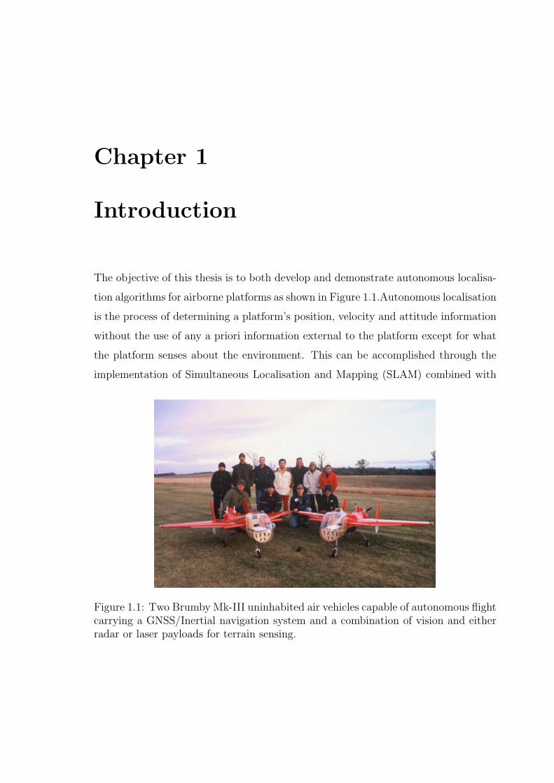
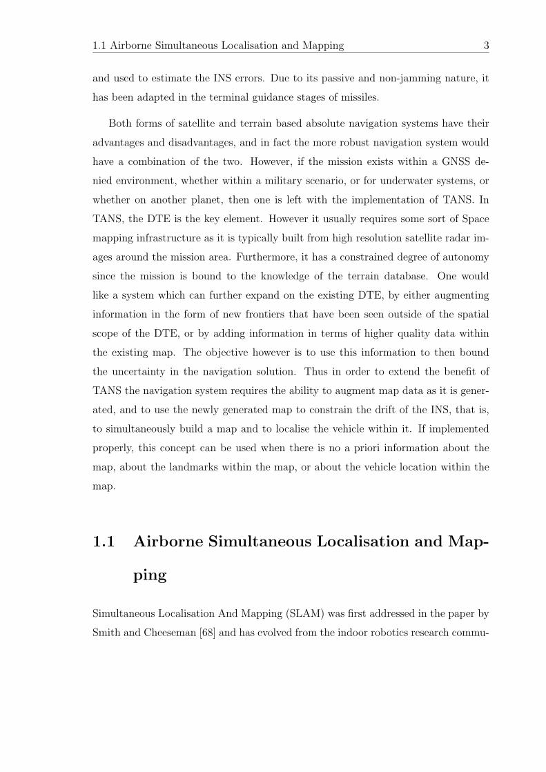
1.1 Two Brumby Mk-III uninhabited air vehicles capable of autonomousflight carrying a GNSS/Inertial navigation system and a combinationof vision and either radar or laser payloads for terrain sensing. . . . . 1
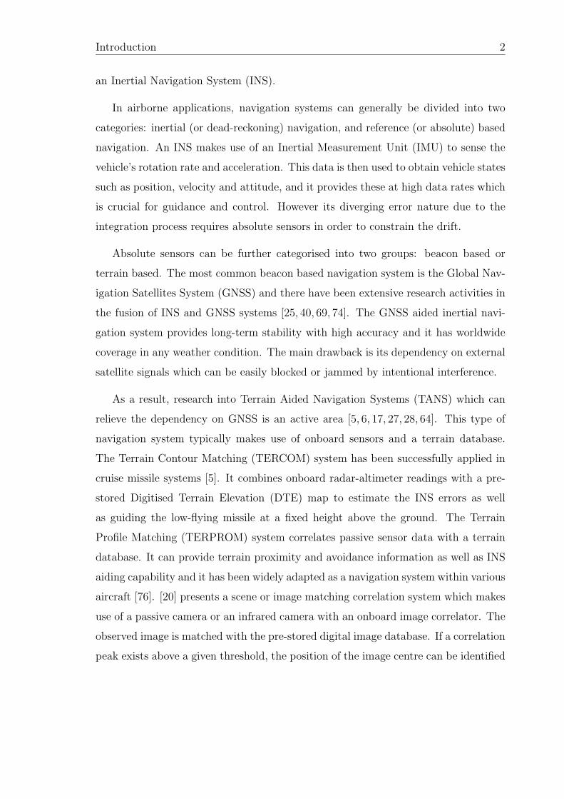
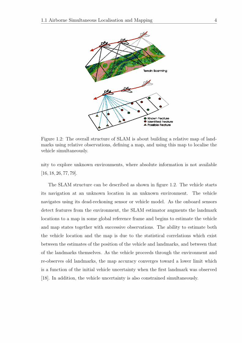
1.2 The overall structure of SLAM is about building a relative map oflandmarks using relative observations, defining a map, and using thismap to localise the vehicle simultaneously. . . . . . . . . . . . . . . . 4
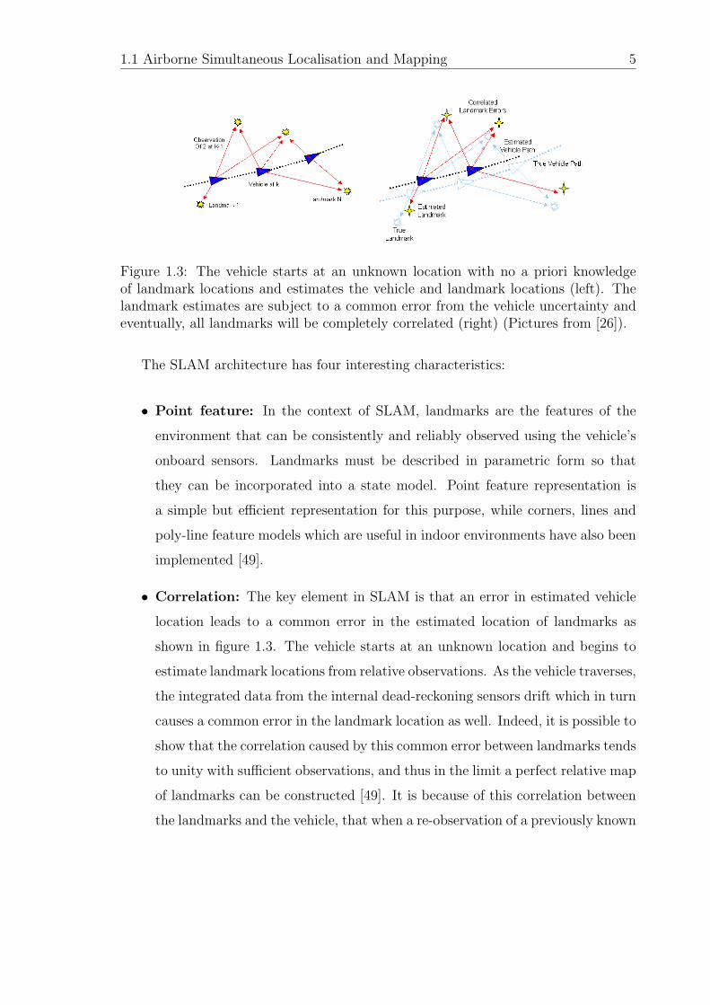
1.3 The vehicle starts at an unknown location with no a priori knowledge oflandmark locations and estimates the vehicle and landmark locations(left). The landmark estimates are subject to a common error from thevehicle uncertainty and eventually, all landmarks will be completelycorrelated (right) (Pictures from [26]). . . . . . . . . . . . . . . . . . 5
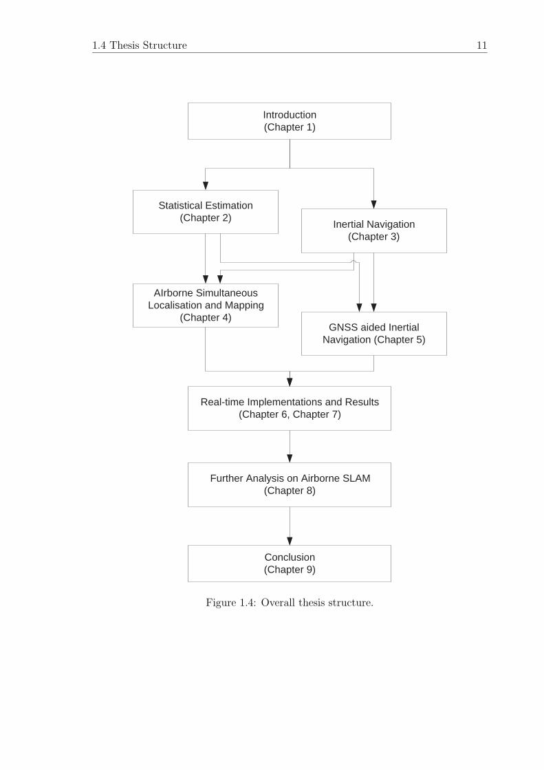
1.4 Overall thesis structure. . . . . . . . . . . . . . . . . . . . . . . . . . 11
2.1 (a) The direct filter configuration and (b) the indirect filter. . . . . . 27
2.2 (a) The direct 6DoF SLAM filter configuration and (b) the indirect one. 30
2.3 The indirect filter configuration of the GNSS/Inertial system. . . . . 32
2.4 The indirect filter configuration of the GNSS/Inertial/Baro system. . 32
3.1 ISIS IMU from Inertial Science, is used to provide 6DoF vehicle infor-mation. . . . . . . . . . . . . . . . . . . . . . . . . . . . . . . . . . . 36
3.2 The position vector in two reference frames with rotational motion. . 50
3.3 IMU lever-arm offset from the centre of gravity of the platform. . . . 59
3.4 The frequency spectrum of acceleration along the y-axis with a 100HzIMU sampling rate with an engine RPM plot. It shows significantaliasing during flight at 8000 RPM, where most of the power spectrumresides in the low frequency region (From flight data on July 2002). . 61
xiii
LIST OF FIGURES xiv
3.5 The frequency spectrum of acceleration along the y-axis with a 400Hzsampling rate. It shows a frequency profile without aliasing duringflight at 8000 RPM (From flight data on April 2003). . . . . . . . . . 61
4.1 The SLAM estimation cycles. . . . . . . . . . . . . . . . . . . . . . . 69
4.2 The range, bearing and elevation observation in the sensor frame canbe related to the location of landmarks in the navigation frame throughthe flight platform’s position and attitude. . . . . . . . . . . . . . . . 75
4.3 (a) Showing the flow chart for direct SLAM implementation and (b)its indirect form. . . . . . . . . . . . . . . . . . . . . . . . . . . . . . 86
4.4 (a) A DDF data fusion structure. Each sensor node incorporates asensor, local processor, and communication capabilities. (b) A DDFSLAM sensor node structure with channel filter, channel manager andSLAM filter. . . . . . . . . . . . . . . . . . . . . . . . . . . . . . . . . 97
4.5 DDF SLAM: Multiple platforms use 6DoF SLAM as their DDF nodesand contribute a common map by exchanging maps. The common mapis also used to navigate simultaneously (Picture from [59]). . . . . . . 98
5.1 The indirect filter configuration of the GNSS/Inertial system. . . . . 105
5.2 (a) The strong correlation between the GNSS velocity and the veloc-ity derived from the position, indicates that the GNSS velocity is anaverage velocity with a 0.5s delay. (b) is the enhanced plots on thebanking and (c) is for the level flight. . . . . . . . . . . . . . . . . . 112
5.3 GNSS vulnerability in altitude from a real-time flight test on July 2,2002. (a) The GNSS receiver with its antenna on the left wing ofthe vehicle shows a fault in altitude. The accumulated error in GNSSaltitude reached up to 180m. (b) Two GNSS antennae have differentsatellite sky views. . . . . . . . . . . . . . . . . . . . . . . . . . . . . 119
5.4 Enhanced view of GNSS fault in altitude. (a) After the height fixedmode, the GNSS height failed to converge to truth due to successiveshadings in the GNSS signal. (b) The error reached to 180m even in3D mode with 6 satellite vehicles. . . . . . . . . . . . . . . . . . . . . 120
5.5 The indirect filter configuration of the GNSS/Inertial/Baro system. . 122
5.6 The error in the baro-altimeter is modelled by a Markov process witha time constant (β) and a noise strength (σ). . . . . . . . . . . . . . . 123
6.1 The four Brumby Mk-III airframes used for the ANSER demonstrations.127
LIST OF FIGURES xv
6.2 (a) The original Brumby Mk-I airframe. (b) The Brumby Mk-III air-frame on the runway at the flight test facility (Left), and Mr JeremyRandle, the UAV engineer responsible for the design, construction andmaintenance of the aircraft, gives some perspective to its true size(Right). . . . . . . . . . . . . . . . . . . . . . . . . . . . . . . . . . . 128
6.3 The lever-arms of the on-board sensors on the Brumby Mk-III. . . . . 130
6.4 One of GPS receivers mounted on a PC104 carrier board on the FCC. 132
6.5 Two GPS antennae are installed permanently under a layer of carbonfibre in each wing. . . . . . . . . . . . . . . . . . . . . . . . . . . . . 132
6.6 The differential GPS antenna is installed on the roof of the shed at thetest site with a Novatel RT20 GPS receiver. . . . . . . . . . . . . . . 133
6.7 A view from the rear hatch of the fuselage. The air data system whichconsists of a FlexIOTM card and electronics can be seen next to thefuel tank. . . . . . . . . . . . . . . . . . . . . . . . . . . . . . . . . . 134
6.8 Two AccuStarTM inclinometers are used to calibrate the turn-on biasesin the accelerometers. . . . . . . . . . . . . . . . . . . . . . . . . . . . 135
6.9 A small Sony CCS-SONY-HR camera is used as the vision system. Itis installed next to the IMU pointing downward. . . . . . . . . . . . . 135
6.10 Typical images from the camera payload. The white artificial featuresare visible in the upper and lower left frames. The top right frameshows a white 4-wheel drive in the image which was used to test per-formance with moving features. The bottom right frame is taken overone of the dams on the test facility which could easily be used as anatural feature. . . . . . . . . . . . . . . . . . . . . . . . . . . . . . . 136
6.11 A vision/laser system is installed in the front nose pointing downward.A dual processor systems to process the observation and the SLAMseparately can be seen on top of the vision/laser sensor . . . . . . . . 138
6.12 A millimetre wave radar with 2-axes gimballed scanner is installed inthe front nose of Brumby Mk-III. . . . . . . . . . . . . . . . . . . . . 138
6.13 The overall functional diagram of the navigation, guidance and controlloop implemented in the FCC. . . . . . . . . . . . . . . . . . . . . . . 140
6.14 Sensor connection diagram in the flight control computer (picture canbe provided upon request). . . . . . . . . . . . . . . . . . . . . . . . . 141
6.15 Time synchronisation in the ANSER system (picture can be providedupon request). . . . . . . . . . . . . . . . . . . . . . . . . . . . . . . . 141
LIST OF FIGURES xvi
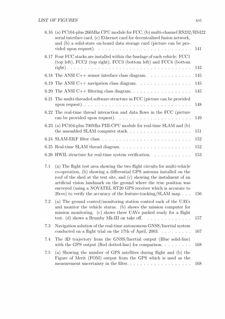
6.16 (a) PC104-plus 266Mhz CPU module for FCC, (b) multi-channel RS232/RS422serial interface card, (c) Ethernet card for decentralised fusion network,and (b) a solid-state on-board data storage card (picture can be pro-vided upon request). . . . . . . . . . . . . . . . . . . . . . . . . . . . 141
6.17 Four FCC stacks are installed within the fuselage of each vehicle: FCC1(top left), FCC2 (top right), FCC3 (bottom left) and FCC4 (bottomright) . . . . . . . . . . . . . . . . . . . . . . . . . . . . . . . . . . . . 142
6.18 The ANSI C++ sensor interface class diagram. . . . . . . . . . . . . 145
6.19 The ANSI C++ navigation class diagram. . . . . . . . . . . . . . . . 145
6.20 The ANSI C++ filtering class diagram. . . . . . . . . . . . . . . . . . 145
6.21 The multi-threaded software structure in FCC (picture can be providedupon request). . . . . . . . . . . . . . . . . . . . . . . . . . . . . . . . 148
6.22 The real-time thread interaction and data flows in the FCC (picturecan be provided upon request). . . . . . . . . . . . . . . . . . . . . . 149
6.23 (a) PC104-plus 700Mhz PIII-CPU module for real-time SLAM and (b)the assembled SLAM computer stack. . . . . . . . . . . . . . . . . . . 151
6.24 SLAM-EKF filter class. . . . . . . . . . . . . . . . . . . . . . . . . . . 152
6.25 Real-time SLAM thread diagram. . . . . . . . . . . . . . . . . . . . . 152
6.26 HWIL structure for real-time system verification. . . . . . . . . . . . 153
7.1 (a) The flight test area showing the two flight circuits for multi-vehicleco-operation, (b) showing a differential GPS antenna installed on theroof of the shed at the test site, and (c) showing the instalment of anartificial vision landmark on the ground where the true position wassurveyed (using a NOVATEL RT20 GPS receiver which is accurate to20cm) to verify the accuracy of the feature-tracking/SLAM map. . . . 156
7.2 (a) The ground control/monitoring station control each of the UAVsand monitor the vehicle status. (b) shows the mission computer formission monitoring. (c) shows three UAVs parked ready for a flighttest. (d) shows a Brumby Mk-III on take off. . . . . . . . . . . . . . 157
7.3 Navigation solution of the real-time autonomous GNSS/Inertial systemconducted on a flight trial on the 17th of April, 2003. . . . . . . . . . 167
7.4 The 3D trajectory from the GNSS/Inertial output (Blue solid-line)with the GPS output (Red dotted-line) for comparison. . . . . . . . . 168
7.5 (a) Showing the number of GPS satellites during flight and (b) theFigure of Merit (FOM) output from the GPS which is used as themeasurement uncertainty in the filter. . . . . . . . . . . . . . . . . . . 168
LIST OF FIGURES xvii
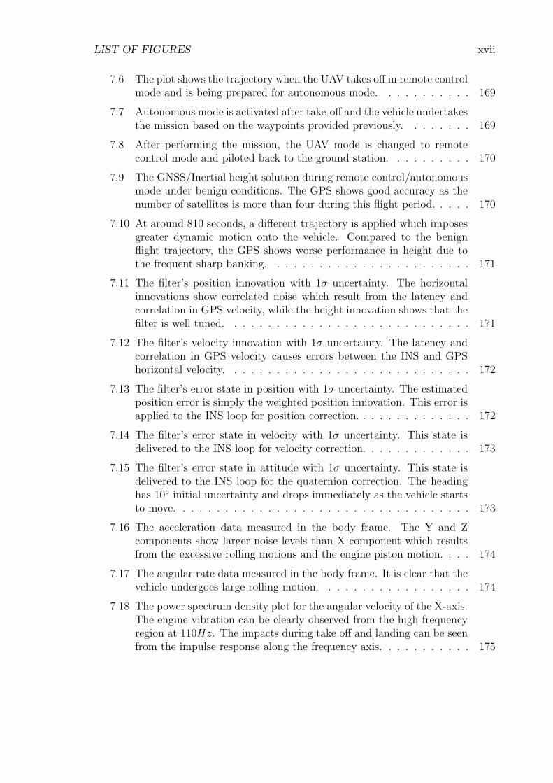
7.6 The plot shows the trajectory when the UAV takes off in remote controlmode and is being prepared for autonomous mode. . . . . . . . . . . 169
7.7 Autonomous mode is activated after take-off and the vehicle undertakesthe mission based on the waypoints provided previously. . . . . . . . 169
7.8 After performing the mission, the UAV mode is changed to remotecontrol mode and piloted back to the ground station. . . . . . . . . . 170
7.9 The GNSS/Inertial height solution during remote control/autonomousmode under benign conditions. The GPS shows good accuracy as thenumber of satellites is more than four during this flight period. . . . . 170
7.10 At around 810 seconds, a different trajectory is applied which imposesgreater dynamic motion onto the vehicle. Compared to the benignflight trajectory, the GPS shows worse performance in height due tothe frequent sharp banking. . . . . . . . . . . . . . . . . . . . . . . . 171
7.11 The filter’s position innovation with 1σ uncertainty. The horizontalinnovations show correlated noise which result from the latency andcorrelation in GPS velocity, while the height innovation shows that thefilter is well tuned. . . . . . . . . . . . . . . . . . . . . . . . . . . . . 171
7.12 The filter’s velocity innovation with 1σ uncertainty. The latency andcorrelation in GPS velocity causes errors between the INS and GPShorizontal velocity. . . . . . . . . . . . . . . . . . . . . . . . . . . . . 172
7.13 The filter’s error state in position with 1σ uncertainty. The estimatedposition error is simply the weighted position innovation. This error isapplied to the INS loop for position correction. . . . . . . . . . . . . . 172
7.14 The filter’s error state in velocity with 1σ uncertainty. This state isdelivered to the INS loop for velocity correction. . . . . . . . . . . . . 173
7.15 The filter’s error state in attitude with 1σ uncertainty. This state isdelivered to the INS loop for the quaternion correction. The headinghas 10◦ initial uncertainty and drops immediately as the vehicle startsto move. . . . . . . . . . . . . . . . . . . . . . . . . . . . . . . . . . . 173
7.16 The acceleration data measured in the body frame. The Y and Zcomponents show larger noise levels than X component which resultsfrom the excessive rolling motions and the engine piston motion. . . . 174
7.17 The angular rate data measured in the body frame. It is clear that thevehicle undergoes large rolling motion. . . . . . . . . . . . . . . . . . 174
7.18 The power spectrum density plot for the angular velocity of the X-axis.The engine vibration can be clearly observed from the high frequencyregion at 110Hz. The impacts during take off and landing can be seenfrom the impulse response along the frequency axis. . . . . . . . . . . 175
LIST OF FIGURES xviii
7.19 The profile of the engine RPM during the flight test. . . . . . . . . . 175
7.20 The baro-altimeter augmented GNSS/Inertial results in a horizontalposition solution which is almost identical to the GNSS/Inertial position.176
7.21 The height of the GNSS/Inertial/Baro system during climbing andafter take-off. The GPS, baro-altimeter and GNSS/Inertial results areplotted together for comparison. The GPS height data is ignored in thefilter by assigning a large observation noise and only the baro-altimeteris used for height aiding. . . . . . . . . . . . . . . . . . . . . . . . . . 177
7.22 The height of GNSS/Inertial/Baro system during remote control mode.The baro-altimeter shows some errors when the vehicle descends. Thereason was not clear, however the pressure sensors seemed not to befirmly attached and hence affected by the vehicle dynamics. . . . . . 177
7.23 The height of the GNSS/Inertial/Baro system during autonomous mode.The high banking command from the guidance loop caused errors inthe GNSS height and GNSS/Inertial as well, while the baro-aided sys-tem showed a more reliable result. . . . . . . . . . . . . . . . . . . . . 178
7.24 The height of the GNSS/Inertial/Baro system during manual controland landing. . . . . . . . . . . . . . . . . . . . . . . . . . . . . . . . . 178
7.25 The 2D horizontal position result of the INS/Vision SLAM systemusing real IMU and vision data. . . . . . . . . . . . . . . . . . . . . . 179
7.26 The 3D position result of the INS/Vision SLAM system. . . . . . . . 180
7.27 The 3D velocity result of the INS/Vision SLAM system. . . . . . . . 180
7.28 The 3D attitude result of the INS/Vision SLAM system. . . . . . . . 181
7.29 The INS/Vision SLAM filter innovation in range, bearing, and elevation.181
7.30 The evolution of the map and vehicle covariance along the North axiswith 1σ uncertainties. . . . . . . . . . . . . . . . . . . . . . . . . . . . 182
7.31 The evolution of the map and vehicle covariance along the East positionwith 1σ uncertainties. . . . . . . . . . . . . . . . . . . . . . . . . . . . 182
7.32 The evolution of the map and vehicle uncertainties (1σ) along the Downaxis. . . . . . . . . . . . . . . . . . . . . . . . . . . . . . . . . . . . . 183
7.33 The final map uncertainties (1σ). The large uncertainty occurred fromspurious observations during banking. . . . . . . . . . . . . . . . . . . 183
7.34 The vehicle and landmark positions estimated from the real-time SLAMsystem. The GNSS/Inertial position and surveyed landmark posi-tions are plotted for comparison, showing the correspondences withthe ground truths. . . . . . . . . . . . . . . . . . . . . . . . . . . . . 184
LIST OF FIGURES xix
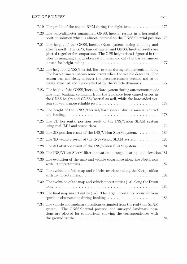
7.35 The SLAM estimated vehicle height with 1σ uncertainty. . . . . . . . 185
7.36 The final landmark positions with 1σ uncertainties provided by real-time SLAM system. . . . . . . . . . . . . . . . . . . . . . . . . . . . . 185
7.37 The detailed views of real-time SLAM during the first round. (a) TheSLAM system was activated during the flight. (b),(c) and (d) presentthe incremental building up of the map and used it to estimate inertialerrors simultaneously (5σ ellipses were plotted for the landmark). . . 186
7.38 The detailed views of real-time SLAM during the round. (a) Thevehicle re-approaches the initial position and (b) the loop is closed byobserving earlier landmarks. The map accuracy improved and alongwith the vehicle’s states. (c) and (d) show accuracy improvements forsuccessive re-observations of landmarks within the round. . . . . . . . 187
7.39 Detailed views of real-time SLAM after the second round. (a) Thevehicle re-approaches the initial position for the second round. In (b)and (c) the loop is closed for the second time. In (d) further loopsimprove the accuracy although minimally. . . . . . . . . . . . . . . . 188
7.40 (a) The bearing and elevation angle and (b) the range (with the uncer-tainty) from the vision node during the real-time SLAM demonstration.189
7.41 The evolution of the vehicle and map uncertainties (1σ) along the northaxis. The effect of closing the loop can be observed around 170, 300and 440 seconds, where the vehicle uncertainty shrinks to its initialvalue. The improvement of the vehicle around 100 seconds resultedfrom successive landmark observations in different view angles. . . . . 189
7.42 The evolution of the vehicle and map uncertainties (1σ) along the eastaxis. As in the north position, the effect of closing the loop can beobserved at around 170, 300 and 440 seconds. . . . . . . . . . . . . . 190
7.43 The evolution of vehicle and map uncertainties (1σ) along the downaxis. Similar patterns are seen along the other axes. However, thelarger uncertainty in vision range compared to the bearing and ele-vation angles causes greater inaccuracy in the map along the verticalaxis. . . . . . . . . . . . . . . . . . . . . . . . . . . . . . . . . . . . . 190
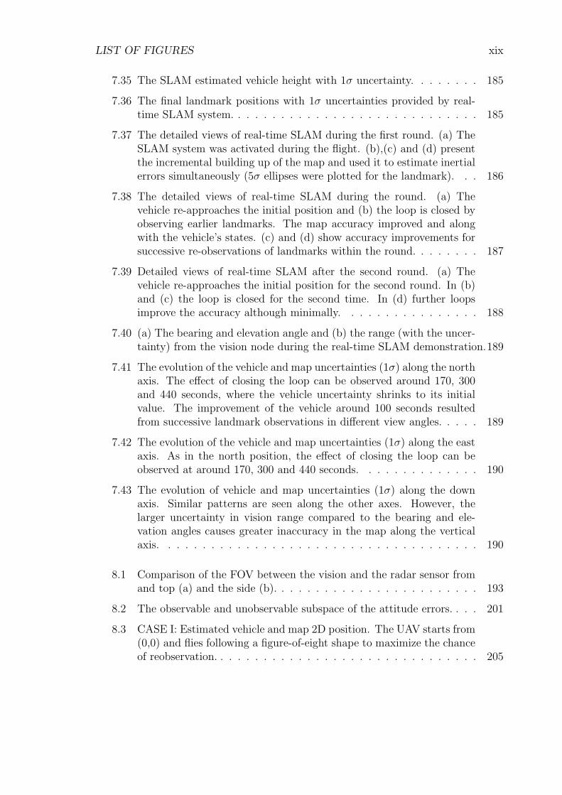
8.1 Comparison of the FOV between the vision and the radar sensor fromand top (a) and the side (b). . . . . . . . . . . . . . . . . . . . . . . . 193
8.2 The observable and unobservable subspace of the attitude errors. . . . 201
8.3 CASE I: Estimated vehicle and map 2D position. The UAV starts from(0,0) and flies following a figure-of-eight shape to maximize the chanceof reobservation. . . . . . . . . . . . . . . . . . . . . . . . . . . . . . . 205
LIST OF FIGURES xx
8.4 CASE I: Enhanced view of vehicle and map 2D position at reobserva-tion. The accumulated vehicle errors are corrected with a discontinuityof 20m around the start area. . . . . . . . . . . . . . . . . . . . . . . 206
8.5 CASE I: Position error with estimated 1σ uncertainty. Due to thelimited view of the vision camera, the errors grow up to 20m. . . . . . 206
8.6 CASE I: Velocity error with estimated 1σ uncertainty. . . . . . . . . . 207
8.7 CASE I: Attitude error with estimated 1σ uncertainty. It can be seenthat the initial alignment error along the roll and pitch axes are esti-mated within the first 50 seconds and the heading uncertainty beginsto be observable after reobservation at around 90 seconds. . . . . . . 207
8.8 CASE I: Evolution of the vehicle covariance (solid line) and landmarks(thin line) along the north position. The first two rounds are theregistration stage for unknown landmarks so the map accuracy haspoor quality. However after the 3rd round, it can be observed that themap accuracy is improved, suppressing the INS drifts. . . . . . . . . . 208
8.9 CASE I: Final mapping performance achieved from the SLAM algo-rithm. The final landmark accuracy is under 6m with the initial vehicleuncertainty of 5m. . . . . . . . . . . . . . . . . . . . . . . . . . . . . 208
8.10 CASE II: Estimated vehicle and map 2D position. The radar sensorhas a wider FOV and the resulting SLAM trajectory shows greaterconsistency than in the vision case. . . . . . . . . . . . . . . . . . . . 209
8.11 CASE II: Position error with estimated 1σ uncertainty. The positionuncertainty is maintained around the initial INS position uncertaintyof 5m. . . . . . . . . . . . . . . . . . . . . . . . . . . . . . . . . . . . 210
8.12 CASE II: Velocity error with estimated 1σ uncertainty. . . . . . . . . 210
8.13 CASE II: Attitude error with estimated 1σ uncertainty. . . . . . . . . 211
8.14 CASE II: Innovation sequences with estimated covariances for range,bearing and elevation indicates proper EKF SLAM operation. . . . . 211
8.15 CASE II: Evolution of the north position covariance of the vehicle andthe landmarks. In the first two rounds, the landmarks are registeredusing the vehicle state and observation then afterwards the vehiclemakes use of the landmarks to suppress the INS drifts. . . . . . . . . 212
8.16 CASE II: Enhanced view of the covariance along the north positionduring the first two rounds. Due to the long range and nonlinearity inthe radar sensor, the initialised landmarks show large uncertainties. . 212
LIST OF FIGURES xxi
8.17 CASE II: Enhanced view of the north position covariance of the vehicleand map after the third round. In this round, due to the previousreobservation effect and wide FOV of radar, the accuracy of vehicleand landmarks are maintained under 5.2m. . . . . . . . . . . . . . . 213
8.18 CASE II: Final mapping performance achieved from the SLAM algo-rithm. The overall landmarks show 5.2m accuracy. . . . . . . . . . . . 213
8.19 The indirect SLAM result with the estimated vehicle and map position(1σ ellipsoids were used). The UAV starts at (0,0) and traverses in afigure eight. . . . . . . . . . . . . . . . . . . . . . . . . . . . . . . . . 214
8.20 A comparison of the vehicle’s position errors under direct and indirectSLAM. . . . . . . . . . . . . . . . . . . . . . . . . . . . . . . . . . . 215
8.21 A comparison of the vehicle’s velocity errors under direct and indirectSLAM. . . . . . . . . . . . . . . . . . . . . . . . . . . . . . . . . . . . 215
8.22 A comparison of the vehicle’s attitude errors under direct and the in-direct SLAM. . . . . . . . . . . . . . . . . . . . . . . . . . . . . . . . 216
8.23 A comparison of the 5th landmark’s uncertainty (1σ) in the northdirection. . . . . . . . . . . . . . . . . . . . . . . . . . . . . . . . . . 216
8.24 A comparison of the north position error with its (1σ) uncertainty withthree different filter prediction rates of 400Hz, 100Hz and 10Hz (Theresults are almost identical to each other). . . . . . . . . . . . . . . . 217
8.25 A comparison of the north velocity error with its (1σ) uncertainty withthree different filter prediction rates of 400Hz, 100Hz and 10Hz. . . . 217
8.26 A comparison of the heading error with its (1σ) uncertainty with threedifferent filter prediction rates of 400Hz, 100Hz and 10Hz. . . . . . . 218
8.27 A comparison of the 5th landmark’s uncertainty (1σ) along the northdirection with three different filter prediction rates of 400Hz, 100Hzand 10Hz. . . . . . . . . . . . . . . . . . . . . . . . . . . . . . . . . . 218
8.28 6DoF DDF SLAM result in UAV-1 with (a) the estimated vehicle andlandmark position (5σ ellipsoids were used for clarification) and (b)the final landmark uncertainty. Since UAV-2 flies the other part of thefigure-of-eight and there is communication of maps, the resulting mapincludes additional landmarks in the area. The large uncertainty inlandmark 3 was due to the high bank angle during observation. . . . 219
8.29 6DoF DDF SLAM result in UAV-2 with (a) the estimated vehicle andlandmark position and (b) the final landmark uncertainty. Due to mapcommunication, both UAVs build a common combined map. . . . . . 219
LIST OF FIGURES xxii
8.30 Standalone SLAM result in UAV-1 with (a) the position and (b) thefinal landmark uncertainty. The resulting map contains only 11 land-marks with a larger uncertainty than the DDF map (Landmark 9 withlarge uncertainty corresponds to the landmark 3 in the DDF map). . 220
8.31 Standalone SLAM result in UAV-2 with (a) the position and (b) thefinal landmark uncertainty. The resulting map contains only 8 land-marks with larger uncertainty than the DDF map. . . . . . . . . . . . 220
8.32 Comparison of the position uncertainties along the north axis in (a)UAV-1 and (b) UAV-2 with (dash line) and without (solid line) mapcommunications. The enhancement of map in DDF mode improvedboth vehicle positions as well. . . . . . . . . . . . . . . . . . . . . . . 221
8.33 Comparison of the attitude uncertainties along the heading axis in(a) UAV-1 and (b) UAV-2 with (dash line) and without (solid line)DDF communications. It can be seen that in DDF mode, both vehicleattitudes are also improved (the rapid decrease of heading uncertaintyin UAV-1 was due to the high maneuvers at the start which enhancedthe heading observability on UAV-1, while UAV-2 undergoes relativelylow maneuvers at the start). . . . . . . . . . . . . . . . . . . . . . . . 221
List of Tables
3.1 The engine RPM profile during the flight test . . . . . . . . . . . . . . 64
3.2 The magnitudes of the coning drift rates computed in different conditions. 65
5.1 The lever-arm parameters and the flight characteristics. . . . . . . . . 117
5.2 The lever-arm’s error contributions to the filter observations. . . . . . 117
6.1 The Brumby performance characteristics. . . . . . . . . . . . . . . . . 129
6.2 The IMU specification. . . . . . . . . . . . . . . . . . . . . . . . . . . 131
6.3 The CMC-Allstar GPS receiver specification. . . . . . . . . . . . . . . 132
7.1 GNSS/Inertial navigation performance (1σ) on 17th April 2003. . . . 160
8.1 The simulation parameters used in SLAM with vision, radar, and vi-sion/laser. . . . . . . . . . . . . . . . . . . . . . . . . . . . . . . . . . 194
8.2 The SLAM performances in CASE I and CASE II. . . . . . . . . . . 196
8.3 The results of the indirect SLAM navigation. . . . . . . . . . . . . . . 197
xxiii
Chapter 1
Introduction
The objective of this thesis is to both develop and demonstrate autonomous localisa-
tion algorithms for airborne platforms as shown in Figure 1.1.Autonomous localisation
is the process of determining a platform’s position, velocity and attitude information
without the use of any a priori information external to the platform except for what
the platform senses about the environment. This can be accomplished through the
implementation of Simultaneous Localisation and Mapping (SLAM) combined with
Figure 1.1: Two Brumby Mk-III uninhabited air vehicles capable of autonomous flightcarrying a GNSS/Inertial navigation system and a combination of vision and eitherradar or laser payloads for terrain sensing.
Introduction 2
an Inertial Navigation System (INS).
In airborne applications, navigation systems can generally be divided into two
categories: inertial (or dead-reckoning) navigation, and reference (or absolute) based
navigation. An INS makes use of an Inertial Measurement Unit (IMU) to sense the
vehicle’s rotation rate and acceleration. This data is then used to obtain vehicle states
such as position, velocity and attitude, and it provides these at high data rates which
is crucial for guidance and control. However its diverging error nature due to the
integration process requires absolute sensors in order to constrain the drift.
Absolute sensors can be further categorised into two groups: beacon based or
terrain based. The most common beacon based navigation system is the Global Nav-
igation Satellites System (GNSS) and there have been extensive research activities in
the fusion of INS and GNSS systems [25, 40, 69, 74]. The GNSS aided inertial navi-
gation system provides long-term stability with high accuracy and it has worldwide
coverage in any weather condition. The main drawback is its dependency on external
satellite signals which can be easily blocked or jammed by intentional interference.
As a result, research into Terrain Aided Navigation Systems (TANS) which can
relieve the dependency on GNSS is an active area [5, 6, 17, 27, 28, 64]. This type of
navigation system typically makes use of onboard sensors and a terrain database.
The Terrain Contour Matching (TERCOM) system has been successfully applied in
cruise missile systems [5]. It combines onboard radar-altimeter readings with a pre-
stored Digitised Terrain Elevation (DTE) map to estimate the INS errors as well
as guiding the low-flying missile at a fixed height above the ground. The Terrain
Profile Matching (TERPROM) system correlates passive sensor data with a terrain
database. It can provide terrain proximity and avoidance information as well as INS
aiding capability and it has been widely adapted as a navigation system within various
aircraft [76]. [20] presents a scene or image matching correlation system which makes
use of a passive camera or an infrared camera with an onboard image correlator. The
observed image is matched with the pre-stored digital image database. If a correlation
peak exists above a given threshold, the position of the image centre can be identified
1.1 Airborne Simultaneous Localisation and Mapping 3
and used to estimate the INS errors. Due to its passive and non-jamming nature, it
has been adapted in the terminal guidance stages of missiles.
Both forms of satellite and terrain based absolute navigation systems have their
advantages and disadvantages, and in fact the more robust navigation system would
have a combination of the two. However, if the mission exists within a GNSS de-
nied environment, whether within a military scenario, or for underwater systems, or
whether on another planet, then one is left with the implementation of TANS. In
TANS, the DTE is the key element. However it usually requires some sort of Space
mapping infrastructure as it is typically built from high resolution satellite radar im-
ages around the mission area. Furthermore, it has a constrained degree of autonomy
since the mission is bound to the knowledge of the terrain database. One would
like a system which can further expand on the existing DTE, by either augmenting
information in the form of new frontiers that have been seen outside of the spatial
scope of the DTE, or by adding information in terms of higher quality data within
the existing map. The objective however is to use this information to then bound
the uncertainty in the navigation solution. Thus in order to extend the benefit of
TANS the navigation system requires the ability to augment map data as it is gener-
ated, and to use the newly generated map to constrain the drift of the INS, that is,
to simultaneously build a map and to localise the vehicle within it. If implemented
properly, this concept can be used when there is no a priori information about the
map, about the landmarks within the map, or about the vehicle location within the
map.
1.1 Airborne Simultaneous Localisation and Map-
ping
Simultaneous Localisation And Mapping (SLAM) was first addressed in the paper by
Smith and Cheeseman [68] and has evolved from the indoor robotics research commu-
1.1 Airborne Simultaneous Localisation and Mapping 4
Figure 1.2: The overall structure of SLAM is about building a relative map of land-marks using relative observations, defining a map, and using this map to localise thevehicle simultaneously.
nity to explore unknown environments, where absolute information is not available
[16, 18, 26, 77, 79].
The SLAM structure can be described as shown in figure 1.2. The vehicle starts
its navigation at an unknown location in an unknown environment. The vehicle
navigates using its dead-reckoning sensor or vehicle model. As the onboard sensors
detect features from the environment, the SLAM estimator augments the landmark
locations to a map in some global reference frame and begins to estimate the vehicle
and map states together with successive observations. The ability to estimate both
the vehicle location and the map is due to the statistical correlations which exist
between the estimates of the position of the vehicle and landmarks, and between that
of the landmarks themselves. As the vehicle proceeds through the environment and
re-observes old landmarks, the map accuracy converges toward a lower limit which
is a function of the initial vehicle uncertainty when the first landmark was observed
[18]. In addition, the vehicle uncertainty is also constrained simultaneously.
1.1 Airborne Simultaneous Localisation and Mapping 5
Figure 1.3: The vehicle starts at an unknown location with no a priori knowledgeof landmark locations and estimates the vehicle and landmark locations (left). Thelandmark estimates are subject to a common error from the vehicle uncertainty andeventually, all landmarks will be completely correlated (right) (Pictures from [26]).
The SLAM architecture has four interesting characteristics:
• Point feature: In the context of SLAM, landmarks are the features of the
environment that can be consistently and reliably observed using the vehicle’s
onboard sensors. Landmarks must be described in parametric form so that
they can be incorporated into a state model. Point feature representation is
a simple but efficient representation for this purpose, while corners, lines and
poly-line feature models which are useful in indoor environments have also been
implemented [49].
• Correlation: The key element in SLAM is that an error in estimated vehicle
location leads to a common error in the estimated location of landmarks as
shown in figure 1.3. The vehicle starts at an unknown location and begins to
estimate landmark locations from relative observations. As the vehicle traverses,
the integrated data from the internal dead-reckoning sensors drift which in turn
causes a common error in the landmark location as well. Indeed, it is possible to
show that the correlation caused by this common error between landmarks tends
to unity with sufficient observations, and thus in the limit a perfect relative map
of landmarks can be constructed [49]. It is because of this correlation between
the landmarks and the vehicle, that when a re-observation of a previously known
1.1 Airborne Simultaneous Localisation and Mapping 6
stationary landmark occurs, then vehicle state estimation can proceed given this
map data.
• Map complexity: The need to maintain these correlations is an integral part
of the SLAM solution. This leads to enormous computational problems, as
the location of each landmark in the environment must, in theory, be updated
at each step in the estimation cycle. To retain all correlations requires O(n3)
computation and O(n2) storage requirement, where n is the number of features,
which is intractable as the size of the operation environment is increased. This
leads inevitably for a need to find effective map management policies for large
scale problems [26, 49].
• Revisiting Landmarks: The most interesting aspect of SLAM is “closing-the-
loop” or the revisiting process. The vehicle’s error grows without bound due to
the drifting nature of the dead-reckoning sensor and this affects the generated
map accuracy as well. However if the vehicle has a chance to revisit a former
registered landmark, the accumulated vehicle error can be estimated which in
turn, improves the overall map accuracy as well. This process makes it possible
to build a perfect relative map of landmarks in the limit.
There have been substantial advances over the recent years in developing the
SLAM algorithm for field robotics particularly for land and underwater vehicles
[26, 77, 79], all of which however assume a flat and 2D environment. The research
conducted has illustrated the problems and remedies associated with the construc-
tion of the algorithm, the requirement for re-observing landmarks for model drift
containment, and issues relating to data association.
In this thesis, the first real-time implementation of the 6DoF SLAM algorithm for
an Uninhibited Air Vehicle (UAV) navigating within a 3D environment is presented,
thus providing a revolutionary step for navigation systems for airborne applications.
1.2 GNSS Aided Airborne Navigation 7
1.2 GNSS Aided Airborne Navigation
The integration of GNSS with an INS has been studied extensively over the decades
and successfully applied to both military and civil areas [25, 40, 69, 74]. The structure
of the GNSS/Inertial system can be broadly categorised into a loosely coupled and a
tightly coupled structure depending on the degree of coupling between the GNSS and
INS [62]. The trend nowadays has been toward deeper levels of integration, where the
INS also aids the GNSS directly with the code and phase frequency tracking-loops [1].
In this thesis, the loosely coupled structure was used by fusing the GNSS position and
velocity data [37, 38, 53]. Although it is a suboptimal structure due to the unknown
correlation information in the GNSS outputs to the integration filter, its main benefit
is that the GNSS and INS systems can be developed independently. Thus various
kinds of off-the-shelf products can be used for the integration with minimum changes.
It can also provide stand-alone functionality and hence redundancy in an integrated
system.
Although the GNSS aided INS is not a primary goal of this thesis (actually it is
used as a reference information to validate the SLAM output), it is still a challenging
area to implement a reliable GNSS/Inertial navigation system using cost effective
sensors. It was also found that within highly dynamic environments, low-cost GNSS
sensors are vulnerable to outages, and hence the INS requires extra aiding, particu-
larly in the form of altitude information. As a solution to this problem the theoretical
and practical aspects of a GNSS/Baro-altimeter aided INS navigation system is stud-
ied in this thesis.
1.3 Contributions
The main contributions of this thesis are:
• The qualification and quantification of errors associated with inertial navigation
systems when implemented in UAV applications.
1.3 Contributions 8
• The development of a direct 6DoF SLAM algorithm using a nonlinear inertial
navigation algorithm and a nonlinear range, bearing and elevation model, thus
expanding the SLAM paradigm to the full 6DoF framework within 3D environ-
ments.
• An analysis of the effect on SLAM performance given different environment
sensors, in particular focusing on a vision and radar sensor with different field-
of-views and observation accuracies.
• The development of an indirect 6DoF SLAM algorithm by formulating a lin-
earised SLAM error model. This allows the SLAM algorithm to be decoupled
from the inertial navigation system and hence provides an efficient filter predic-
tion step (the issues of constant-time SLAM update in terms of map manage-
ment is not addressed in this thesis).
• A comparison of the direct and indirect 6DoF SLAM algorithms, in particular
focusing on how the SLAM prediction rate can be reduced dramatically without
any significant degradations in SLAM performance.
• The further development of Decentralised Data Fusion (DDF) SLAM for mul-
tiple platforms using the 6DoF SLAM implementation.
• The development of a GNSS aided inertial navigation system for a UAV system,
and a baro-altimeter augmented navigation system for the enhancement of alti-
tude accuracy. This includes an understanding and analysis of errors associated
with these sensors.
• The real-time implementation and demonstration of the direct 6DoF SLAM al-
gorithm on a UAV platform using an onboard vision sensor and IMU, presenting
the successful implementation of airborne SLAM.
• The real-time implementation and demonstration of a low-cost GNSS/Inertial
navigation system on a UAV platform. The system provides real-time naviga-
1.4 Thesis Structure 9
tion solutions to the autonomous guidance and control module and is also used
as the truth model for SLAM.
• Finally, an understanding of the observability of 6DoF SLAM using the indirect
SLAM model, in particular focusing on what states are observable and under
what conditions.
1.4 Thesis Structure
The structure of this thesis is outlined in Figure 1.4.
Chapter 2 presents the mathematical background for the statistical estimation
techniques which are used in this thesis. The discrete Kalman filter and information
filter are presented. The structure of the direct and indirect implementations are also
provided. The implementations of these algorithms to the aided inertial navigation
system with either SLAM or GNSS aiding are provided and discussed.
Chapter 3 provides the inertial navigation algorithms which forms the basis of
the aided airborne navigation systems. The equations are formulated in an earth-
fixed local-tangent reference frame. The equations are then perturbed to provide the
error equations for the indirect filter implementation. The placement offset of the
inertial sensor is compensated and the effects of the platform’s vibration are analysed
in detail. Finally, the calibration and alignment methods are provided.
Chapter 4 formulates a 6DoF SLAM algorithm using an IMU and range/bearing
sensor. An indirect SLAM algorithm is then developed. The advantages of this
structure over the direct form are discussed in detail. Finally, the single-vehicle
SLAM algorithm is expanded to the multi-vehicle 6DoF SLAM problem by applying
DDF techniques and sharing the map information between the vehicles, which results
in an improvement of both map quality and localisation of the vehicles.
Chapter 5 formulates an aided inertial navigation system using GNSS and baro-
altimeter. It provides analysis for the GNSS observation latency, synchronisation and
1.4 Thesis Structure 10
lever-arm offset which are crucial in any practical implementation. The vulnerability
of the GNSS altitude are also addressed through the analysis of real flight data, and
as a solution, the baro-altimeter is augmented to the GNSS/Inertial system.
Chapter 6 provides details of the real-time implementations of the SLAM algo-
rithm from Chapter 4 and the GNSS/Inertial algorithm from Chapter 5. The details
of the flight platform and the hardware and software are provided.
Chapter 7 provides the real-time results for the GNSS/Inertial and SLAM navi-
gation systems. The results comprise both post-processed and real-time demonstra-
tions. In particular the focus is on the implementation of the GNSS/Inertial naviga-
tion system, the baro-aided GNSS/Inertial navigation system, and the first real-time
demonstration of 6DoF airborne SLAM.
Chapter 8 provides further analysis into airborne SLAM. There are primarily three
distinct areas which are meant to pave the way for further research:
• The first is to provide results on the indirect versus direct implementations of
SLAM and to demonstrate that minimal loss in performance is attained when
transferring to the indirect implementation,
• the second is to provide a deeper understanding of the performance of SLAM by
comparing the localisation result of SLAM given varying sensor field of views,
and by conducting an observability analysis of SLAM,
• and finally by demonstrating the DDF 6DoF SLAM implementation.
Finally, Chapter 9 provides the conclusion of this thesis along with possible future
research developments.
1.4 Thesis Structure 11
Introduction(Chapter 1)
Real-time Implementations and Results(Chapter 6, Chapter 7)
AIrborne SimultaneousLocalisation and Mapping
(Chapter 4)
Inertial Navigation(Chapter 3)
GNSS aided InertialNavigation (Chapter 5)
Statistical Estimation(Chapter 2)
Conclusion(Chapter 9)
Further Analysis on Airborne SLAM(Chapter 8)
Figure 1.4: Overall thesis structure.
Chapter 2
Statistical estimation
2.1 Introduction
This chapter presents the mathematical foundation and algorithms for the statistical
estimation techniques implemented throughout the thesis along with the way these
algorithms are implemented.
The chapter begins by presenting an overview of Bayesian estimation, which pro-
vides the foundation for the Gaussian based and discrete estimation algorithms im-
plemented throughout the thesis. Such an algorithm is the discrete Kalman filter and
both the linear and non-linear versions of this filter are presented. The chapter will
also provide the discrete information filter which forms the mathematical background
for the decentralised SLAM algorithms. With the estimation algorithms defined, the
chapter will conclude with the way the algorithms are implemented for aiding inertial
navigation systems when either SLAM or GNSS aiding is the focus.
2.2 Bayesian Estimation
The Bayesian filter is a non-linear and non-Gaussian estimation technique which
propagates the probability density function of a random vector over time given a
2.2 Bayesian Estimation 13
probabilistic model of its motion and any observations which are taken of the states
[60].
A state vector x(k) at time k, is assumed to evolve over time with an associated
probability density function P (x(k)), on the state x(k). P (x(k)) is considered a
probabilistic model of the state x(k) before making any observation and hence is
referred to as the a priori distribution.
Probabilistic Motion Model
The probabilistic motion model is defined as a conditional probability distribution on
the state transition in the form [50]
P (x(k) | x(k − 1),u(k)). (2.1)
The state transition is assumed as a Markov process in which the state x(k)
depends only on the immediately preceding state x(k − 1) and the applied control
input u(k). The motion is also assumed to be independent of the observations. This
model describes the probability of the current state based on the information of the
previous state and the control input in a probabilistic sense.
Probabilistic Observation Model
The observation model is defined as a conditional probability density describing the
probability of making an observation z(k), given the known state x(k),
P (z(k) | x(k)). (2.2)
The set of observations Zk up to time k is defined as
Zk = {z(1), z(2), · · · , z(k)} � {Zk−1, z(k)}. (2.3)
2.2 Bayesian Estimation 14
Thus the probability P (x(k) | Zk) is the posterior density on x(k) at time k given
all observations up to time k.
Bayes theorem states that the posteriori density P (x(k) | Zk) can be obtained
from the a priori density and observation model [60]
P (x(k) | Zk) =P (z(k) | x(k))P (x(k) | Zk−1)
P (z(k) | Zk−1)
= C · P (z(k) | x(k))P (x(k) | Zk−1), (2.4)
where C is the normalising factor.
Equation 2.4 forms the heart of the Bayesian estimation problem and it can be
further divided into two separate processes: prediction and update.
Prediction
In Equation 2.4, the density of the current state x(k) given all observations up to
time k− 1 can be found by propagating the density from the previous state x(k− 1)
through the use of a motion model and the control input.
The total probability theorem [60] can be used to rewrite P (x(k) | Zk−1) in
terms of the marginalisation of the joint density of the current and previous state.
Furthermore the joint density can be expressed with the motion model and the a
priori density by applying a chain rule of conditional probability. That is,
P (x(k) | Zk−1) =
∫P (x(k),x(k − 1) | Zk−1)dx
=
∫P (x(k) | x(k − 1),u(k))P (x(k − 1) | Zk−1)dx. (2.5)
2.3 Kalman Filter 15
Estimation
Substituting Equation 2.5 into Equation 2.4 gives
P (x(k) | Zk) = C · P (z(k) | x(k)) ×∫P (x(k) | x(k − 1),u(k))P (x(k − 1) | Zk−1)dx. (2.6)
Equation 2.6 is called the estimation (or update) equation. Upon arrival of a
new observation at time k it calculates the posterior density at time k from the prior
density at time k−1, the motion model, and the observation model. These two steps
of prediction and update in a recursive manner forms the Bayesian filter.
The Bayesian filter, however, cannot be represented in a closed-form due to its
general description of the probability density function. One solution, known as the
particle filter implementation [22], is to approximate the probability density using
multiple samples or particles. As a special case, which will be used within this thesis,
if the system is assumed as linear with the statistical properties being represented by
Gaussian probability functions, then the filter can be expressed in an analytic form
known as the Kalman filter. If non-linear but Gaussian then the extended Kalman
filter is implemented.
2.3 Kalman Filter
If the system is linear and the statistical distribution is Gaussian, then the Bayesian
prediction and update equation can be solved analytically. The system is completely
described by the Gaussian parameters such as mean and covariance and this filter is
called the Kalman filter [51]. As a discrete statistical recursive algorithm, the Kalman
filter provides an estimate of the state at time k given all observations up to time k
and provides an optimal minimal mean squared error estimate of these states.
2.3 Kalman Filter 16
Process Model
A linear dynamic system in discrete time can be described by
x(k) = Fx(k − 1) + Bu(k) + Gw(k), (2.7)
where x(k) is the state vector of interest at time k, F is a linear state transition
matrix which relates the state vector from time k − 1 to k, u(k) is the input control
vector while B relates the control vector to the states, and w(k) is the process noise
injected into the system due to uncertainties in the transition matrix and the control
input while G relates the noise to the states.
The process noise is assumed to be a zero mean, uncorrelated random sequence
with covariance
E[w(k)] = 0 ∀k,
E[w(k)wT (j)] =
⎧⎨⎩ Q(k) k = j
0 k �= j.
Observation Model
When observations of the states are taken, the observation vector z(k) at time k is
given by
z(k) = Hx(k) + v(k), (2.8)
where H is the linear observation model relating the state vector at time k to the
observation vector, and v(k) is the observation noise vector which accounts for the
uncertainty in the observation. The observation noise is also assumed to be a zero
2.3 Kalman Filter 17
mean, uncorrelated random sequence with covariance
E[v(k)] = 0 ∀k,
E[v(k)vT (j)] =
⎧⎨⎩ R(k) k = j
0 k �= j.
It is assumed that the process and observation noise are uncorrelated,
E[w(k)v(j)T ] = 0 ∀k, j.
Given the state dynamic and observation models, the Kalman filter provides a
recursive estimate of the states at time k, x(k | k), given all observations up to time
k.
Prediction
The predicted state is evaluated by taking expectations of Equation 2.7 conditioned
upon the previous k − 1 observations,
x(k | k − 1) � E[x(k | Zk−1)]
= Fx(k − 1 | k − 1) + Bu(k). (2.9)
The uncertainty in the predicted states at time k, P(k | k−1), is described as the
expected value of the variance of the error in the states at time k given all information
up to time k − 1,
P(k | k − 1) � E[(x(k) − x(k | k − 1))(x(k) − x(k | k − 1))T | Zk−1)]
= FP(k − 1 | k − 1)FT + GQ(k)GT . (2.10)
2.3 Kalman Filter 18
Estimation
When an observation from an external aiding sensor is obtained as in Equation 2.8,
an estimate of the state is obtained by,
x(k | k) � E[x(k | Zk)]
= x(k | k − 1) + W(k)ν(k), (2.11)
where W(k) is a gain matrix produced by the Kalman filter and ν(k) is the innovation
vector. The innovation vector is the difference between the actual observation and
the predicted observation. That is,
ν(k) = z(k) − Hx(k | k − 1). (2.12)
The predicted observation is determined by taking the expected value of Equa-
tion 2.8 conditioned on previous observations. Equation 2.11 defines the update as
simply the latest prediction plus a weighting on the innovation. The Kalman gain or
weighting is chosen so as to minimise the mean squared error of the estimate,
W(k) = P(k | k − 1)HTS−1(k), (2.13)
where S(k) is known as the innovation covariance and is obtained by,
S(k) = HP(k | k − 1)HT + R(k). (2.14)
The covariance matrix, or the uncertainty in the updated states, is obtained by
taking the expectation of the variance of the error at time k given all observations up
2.4 Extended Kalman Filter 19
to time k,
P(k | k) � E[(x(k) − x(k | k))(x(k) − x(k | k))T | Zk)]
= [I − W(k)H]P(k | k − 1)[I − W(k)H]T
+W(k)R(k)WT (k). (2.15)
Equation 2.15 is called the Joseph form of the covariance update which assures
the symmetry and positive definiteness of P(k | k), since in this form P(k | k) is
computed as the sum of positive definite and positive semi-definite matrices [51].
2.4 Extended Kalman Filter
In most real applications the process and/or observation models are nonlinear and
hence the linear Kalman filter algorithm described above cannot be directly applied.
To overcome this, a linearised Kalman filter or Extended Kalman Filter (EKF) can
be applied which are estimators where the models are continuously linearised before
applying the estimation techniques [13, 51].
In some applications there exists a predetermined nominal trajectory to navigate.
In this case the nonlinear state model can be linearised around the nominal trajectory
and linear Kalman filter theory can be used. The filter gain which is computationally
expensive can also be computed off-line and can be used as a look-up table in real-time
operation.
However, in most practical navigation applications, a nominal trajectory does not
exist beforehand. The solution is to use the current estimated state from the filter at
each time step k as the linearisation reference from which the estimation procedure
can proceed. Such an algorithm is known as the extended Kalman filter. If the
filter operates properly, the linearisation error around the estimated solution can be
maintained at a reasonably small value. However, if the filter is ill-conditioned due to
2.4 Extended Kalman Filter 20
modelling errors, incorrect tuning of the covariance matrices, or initialisation error,
then the estimation error will affect the linearisation error which in turn will affect
the estimation process and is known as filter divergence. For this reason the EKF
requires greater care in modelling and tuning than the linear Kalman filter.
Nonlinear Process Model
The non-linear dynamic system in discrete time is described by
x(k) = f(x(k − 1),u(k),w(k)), (2.16)
where f(·, ·, ·) is a non-linear state transition function which links the current state
with the previous state and current control input.
Nonlinear Observation Model
The non-linear observation model is represented
z(k) = h(x(k),v(k)), (2.17)
where h(·, ·) is a non-linear observation function which links the observation to the
current state.
Prediction
Following the same definitions outlined in the Kalman filter, the predicted state is
obtained with zero process noise, such as
x(k | k − 1) = f(x(k − 1 | k − 1),u(k),0), (2.18)
2.4 Extended Kalman Filter 21
and the predicted covariance matrix is
P(k | k − 1) = ∇fx(k)P(k − 1 | k − 1)∇fTx (k) + ∇fw(k)Q(k)∇fTw (k), (2.19)
where the term ∇fx(k) is the Jacobian of the non-linear state transition function with
respect to the previous state estimate x(k − 1 | k − 1) and the term ∇fw(k) is the
linearised noise transfer function which corresponds to G in the linear Kalman filter,
and it is computed as the Jacobian with respect to the process noise vector w(k).
Estimation
When an observation occurs, the state vector is updated according to
x(k | k) = x(k | k − 1) + W(k)ν(k), (2.20)
where ν(k) is the innovation vector which is formed by subtracting the predicted
observation with zero observation noise from the measured one, such as
ν(k) = z(k) − h(x(k | k − 1),0). (2.21)
The Kalman gain and innovation covariance are
W(k) = P(k | k − 1)∇hTx (k)S−1(k) (2.22)
S(k) = ∇hx(k)P(k | k − 1)∇hTx (k) + ∇hv(k)R(k)∇hTv (k). (2.23)
where the term ∇hx(k) is the Jacobian of the non-linear observation model with
respect to the previous state estimate x(k − 1 | k − 1) and ∇hv(k) is the Jacobian
with respect to the observation noise v(k).
2.5 Information Filter 22
The updated covariance matrix in Joseph form becomes
P(k | k) = [I − W(k)∇hx(k)]P(k | k − 1)[I − W(k)∇hx(k)]T
+W(k)∇hv(k)R(k)∇hTv (k)WT (k). (2.24)
2.5 Information Filter
The information filter is mathematically equivalent to the Kalman filter except that
it is expressed in terms of measures of information (Fisher information in this thesis)
about the states of interest rather than the direct state and its covariance estimates
[51]. Indeed, the information filter is known to have a dual relationship with the
Kalman filter [2]. If the system is linear with an assumption of Gaussian probability
density distributions, the information matrix Y(k | k), and the information state
estimate y(k | k), are defined in terms of the inverse covariance matrix and state
estimate [55]
Y(k | k) � P−1(k | k) (2.25)
y(k | k) � Y(k | k)x(k | k). (2.26)
When an observation occurs, the information state contribution i(k) and its asso-
ciated information matrix I(k) are
i(k) � HT (k)R−1(k)z(k) (2.27)
I(k) � HT (k)R−1(k)H(k). (2.28)
By using these variables, the information prediction and update equation can be
derived from Kalman filter [55].
2.5 Information Filter 23
Prediction
The predicted information state is obtained by pre-multiplying the information matrix
Y(k | k − 1) in equation 2.9 and by representing it in information space,
y(k | k − 1) = L(k | k − 1)y(k − 1 | k − 1) + Y(k | k − 1)B(k)u(k) (2.29)
where the information propagation coefficient matrix (or the similarity transform
matrix) L(k | k − 1) is given by
L(k | k − 1) = Y(k | k − 1)F(k)Y(k − 1 | k − 1)−1. (2.30)
The corresponding information matrix is obtained by taking the inverse of equa-
tion 2.10 and by representing it in information space,
Y(k | k − 1) =[F(k)Y−1(k − 1 | k − 1)FT (k) + G(k)Q(k)GT (k)
]−1. (2.31)
Estimation
The update procedure is simpler in the information filter than in the Kalman filter.
The observation update is performed by adding the information contribution from
the observation to the information state vector and its matrix
y(k | k) = y(k | k − 1) + i(k) (2.32)
Y(k | k) = Y(k | k − 1) + I(k). (2.33)
If there is more than one observation at time k, the information update is simply
2.5 Information Filter 24
the sum of each information contribution to the state vector and matrix,
y(k | k) = y(k | k − 1) +n∑j=1
ij(k) (2.34)
Y(k | k) = Y(k | k − 1) +n∑j=1
Ij(k), (2.35)
where n is the total number of synchronous observations at time k.
Equation 2.31 can also be represented in a different form by applying the inverse
matrix lemma, which results in a similar form of equation between the information
filter and the Kalman filter [58]. That is, the prediction equations in the information
filter have similar forms with the update equations in the Kalman filter and the update
equations in the information filter with the prediction equations in the Kalman filter.
As the information matrix is defined as the inverse of the covariance matrix, the
information filter deals with the ‘certainty’ rather than ‘uncertainty’ as in the Kalman
filter. Furthermore, given the same number of states, process and observation models,
the computational complexity of the information filter and the Kalman filter are
comparable. The update stage in the information filter is quite simple however the
prediction stage is comparatively complex, which is exactly opposite in the Kalman
filter.
However both filters can show different computational complexity depending on
the dimension of the state and observations. If the number of observations increases,
as in the case of the multi-sensor systems, the dimension of the innovation matrix of
the Kalman filter increases as well, and the inversion of this matrix becomes com-
putationally expensive. In the information filter, however, the information matrix
has the same dimension of the state and its inversion is independent to the size of
observations. This means that the information filter is an efficient algorithm when
the dimension of observations is much greater than that of the state.
In addition, the information filter can perform a synchronous update from multiple
observations in contrast to the Kalman filter. The reason is that the innovations in the
2.6 Extended Information Filter 25
Kalman filter are correlated to the common underlying state while the observation
contributions in the information filter are not. This makes the information filter
attractive in decentralising the filter.
Finally, the information filter can easily be initialised to zero information.
2.6 Extended Information Filter
The extended information filter can also be derived for the non-linear process/observation
model defined in equations 2.16 and 2.17 [55].
Prediction
The predicted information vector and its information matrix are obtained by using
the Jacobians of the non-linear process model
y(k | k − 1) = Y(k | k − 1)f(x(k | k − 1),u(k),0) (2.36)
Y(k | k − 1) = [∇fx(k)Y−1(k − 1 | k − 1)∇fTx (k)
+∇fw(k)Q(k)∇fTw (k)]−1. (2.37)
Estimation
When an observation occurs, the information contribution and its corresponding ma-
trix are
i(k) = ∇hTx (k)[∇hv(k)R(k)∇hTv (k)
]−1[ν(k) + ∇hx(k)x(k | k − 1)] (2.38)
I(k) = ∇hTx (k)[∇hv(k)R(k)∇hTv (k)
]−1 ∇hx(k), (2.39)
2.7 Filter Configurations for Aided Inertial Navigation 26
where the innovation vector is also computed as in the EKF
ν(k) = z(k) − h(x(k | k − 1),0). (2.40)
These information contributions are again added to the information state vector
and matrix as in the linear information filter
y(k | k) = y(k | k − 1) + i(k) (2.41)
Y(k | k) = Y(k | k − 1) + I(k). (2.42)
In most real applications, the nonlinearity of the system makes the EKF/EIF the
only tractable algorithms, since the linearisation process can be performed by using
the estimated states from the filter. The cases with predefined trajectories which can
be used for this linearisation is not considered in this thesis.
Based on these filter algorithms, the integrated navigation system can now be
implemented either directly or indirectly as is presented in the following section.
2.7 Filter Configurations for Aided Inertial Navi-
gation
Within an integrated navigation system, the filter can be configured either as a direct
or indirect form depending on the types of sensors and the complexities of the system
[51]. In a direct configuration, the filter directly estimates the states of interest. It
typically constitutes a main functional block within the system performing both the
dead-reckoning and the observation fusion. In the indirect formulation, the filter
estimates the error quantities of the desired states, and applies this error to the
external dead-reckoning loop for correction, hence it estimate the state indirectly. By
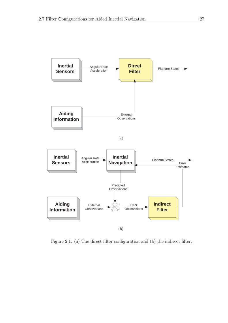
2.7 Filter Configurations for Aided Inertial Navigation 27
InertialSensors
AidingInformation
DirectFilter
Angular RateAcceleration
ExternalObservations
Platform States
(a)
InertialSensors
InertialNavigation
AidingInformation
IndirectFilter
Angular RateAcceleration
ExternalObservations
ErrorEstimates
PredictedObservations
ErrorObservations
Platform States
(b)
Figure 2.1: (a) The direct filter configuration and (b) the indirect filter.
2.7 Filter Configurations for Aided Inertial Navigation 28
dealing with the error quantities, the filter can now be decoupled from the main loop
and can operate in a complementary fashion.
In airborne applications, inertial sensor suites measure acceleration and angular
rates of the platform and are typically incorporated for the dead-reckoning purposes.
These inertial measurements are literally integrated within the Inertial Navigation
System (INS) to obtain the Position, Velocity and Attitude (PVA) of the platform.
Figure 2.1 presents the filter configurations. In the direct filter configuration, the
platform’s PVA are directly estimated from the filter as in figure 2.1(a), whilst they
are the errors in PVA in the indirect configuration as shown in figure 2.1(b).
2.7.1 Advantages and Disadvantages of the Direct and Indi-
rect filter Structures
The advantage of the direct configuration is that the filter output is the required
information and no further processing is required. In some applications such as with
gimballed navigation systems, this can be an effective approach where the mechanical
gimbals provide a stabilised platform for navigation purposes and the filter generates
torque commands only to deal with the small disturbance in the gimbals. In mobile
robot navigation where the dimension of the states is relatively low, it can also be
a suitable configuration. However, for strapdown INS where the inertial sensors are
rigidly attached to the platform body and undergo the same dynamics as the platform,
the direct filter has serious drawbacks. Firstly, the sampling rates of the filter should
be high enough to pick up the vehicle dynamics and to suppress the vibration effects,
typically ranging from 100Hz to several KHz. Coupled with the high dimensionality
of the states (which is at least nine and can further increase depending on the sensor
errors) it can cause a significant computational bottleneck. Secondly, in cases where
system integrity is paramount, and where the design of the filter structure is important
for the reliability of the system, the direct implementation has a serious drawback in
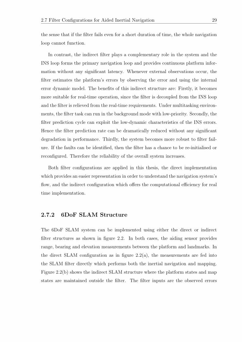
2.7 Filter Configurations for Aided Inertial Navigation 29
the sense that if the filter fails even for a short duration of time, the whole navigation
loop cannot function.
In contrast, the indirect filter plays a complementary role in the system and the
INS loop forms the primary navigation loop and provides continuous platform infor-
mation without any significant latency. Whenever external observations occur, the
filter estimates the platform’s errors by observing the error and using the internal
error dynamic model. The benefits of this indirect structure are: Firstly, it becomes
more suitable for real-time operation, since the filter is decoupled from the INS loop
and the filter is relieved from the real-time requirements. Under multitasking environ-
ments, the filter task can run in the background mode with low-priority. Secondly, the
filter prediction cycle can exploit the low-dynamic characteristics of the INS errors.
Hence the filter prediction rate can be dramatically reduced without any significant
degradation in performance. Thirdly, the system becomes more robust to filter fail-
ure. If the faults can be identified, then the filter has a chance to be re-initialised or
reconfigured. Therefore the reliability of the overall system increases.
Both filter configurations are applied in this thesis, the direct implementation
which provides an easier representation in order to understand the navigation system’s
flow, and the indirect configuration which offers the computational efficiency for real
time implementation.
2.7.2 6DoF SLAM Structure
The 6DoF SLAM system can be implemented using either the direct or indirect
filter structures as shown in figure 2.2. In both cases, the aiding sensor provides
range, bearing and elevation measurements between the platform and landmarks. In
the direct SLAM configuration as in figure 2.2(a), the measurements are fed into
the SLAM filter directly which performs both the inertial navigation and mapping.
Figure 2.2(b) shows the indirect SLAM structure where the platform states and map
states are maintained outside the filter. The filter inputs are the observed errors
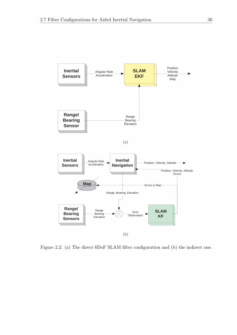
2.7 Filter Configurations for Aided Inertial Navigation 30
Range/BearingSensor
SLAMEKF
Angular RateAcceleration
RangeBearing
Elevation
InertialSensors
PositionVelocityAttitude
Map
(a)
InertialSensors
InertialNavigation
Range/BearingSensors
SLAMKF
Angular RateAcceleration
RangeBearing
Elevation
Position, Velocity, AttitudeErrors
ErrorObservation
Position, Velocity, Attitude
Map Errors in Map
Range, Bearing, Elevation
(b)
Figure 2.2: (a) The direct 6DoF SLAM filter configuration and (b) the indirect one.
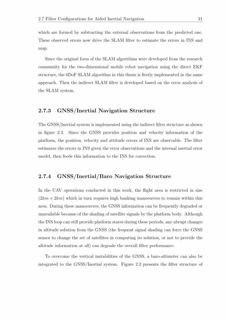
2.7 Filter Configurations for Aided Inertial Navigation 31
which are formed by subtracting the external observations from the predicted one.
These observed errors now drive the SLAM filter to estimate the errors in INS and
map.
Since the original form of the SLAM algorithms were developed from the research
community for the two-dimensional mobile robot navigation using the direct EKF
structure, the 6DoF SLAM algorithm in this thesis is firstly implemented in the same
approach. Then the indirect SLAM filter is developed based on the error analysis of
the SLAM system.
2.7.3 GNSS/Inertial Navigation Structure
The GNSS/Inertial system is implemented using the indirect filter structure as shown
in figure 2.3. Since the GNSS provides position and velocity information of the
platform, the position, velocity and attitude errors of INS are observable. The filter
estimates the errors in INS given the error observations and the internal inertial error
model, then feeds this information to the INS for correction.
2.7.4 GNSS/Inertial/Baro Navigation Structure
In the UAV operations conducted in this work, the flight area is restricted in size
(2km× 2km) which in turn requires high banking manoeuvres to remain within this
area. During these manoeuvres, the GNSS information can be frequently degraded or
unavailable because of the shading of satellite signals by the platform body. Although
the INS loop can still provide platform states during these periods, any abrupt changes
in altitude solution from the GNSS (the frequent signal shading can force the GNSS
sensor to change the set of satellites in computing its solution, or not to provide the
altitude information at all) can degrade the overall filter performance.
To overcome the vertical instabilities of the GNSS, a baro-altimeter can also be
integrated to the GNSS/Inertial system. Figure 2.3 presents the filter structure of
2.7 Filter Configurations for Aided Inertial Navigation 32
InertialSensors
InertialNavigation
GNSS KF
Angular RateAcceleration
PositionVelocity
Errors inPosition, Velocity, Attitude
PositionVelocity
ErrorObservation
Position, Velocity, Attitude
Figure 2.3: The indirect filter configuration of the GNSS/Inertial system.
InertialSensors
InertialNavigation
GNSS
KF
Angular RateAcceleration
PositionVelocity
Errors inPosition, Velocity, Attitude
PositionVelocity
Pos/VelError
Position, Velocity, Attitude
Baro-altimeter
Altitude Altitude Error
Altitude
Figure 2.4: The indirect filter configuration of the GNSS/Inertial/Baro system.
2.8 Summary 33
the baro-augmented GNSS/Inertial system. The filter structure runs in a multi-rate
fashion whenever the GNSS and baro-altimeter observations occurs and provides error
estimates to the INS loop.
2.8 Summary
This chapter has provided the statistical estimation algorithms which are used within
this thesis. The Bayesian filter was introduced based on general probability density
functions. The discrete equations for the linear and extended Kalman filter were
presented as a special form of the Bayesian filter where both linearity and Gaussian
assumptions are made. The information filter was also presented by defining the
information state and the information matrix. Finally, the filter structures which
implement these algorithms and that are used throughout this thesis were then pre-
sented. The benefits of the indirect filter structure were discussed and compared to
the direct state filter structure.
Chapter 3
Strapdown Inertial Navigation
3.1 Introduction
Almost all airborne navigation systems incorporate an Inertial Navigation System
(INS) with an Inertial Measurement Unit (IMU) being the dead-reckoning system to
compute the navigation information of the platform required. This is due to the high
data rates available which are important for highly dynamic systems, and because
the information provided is of the full 6 Degrees-of-Freedom (DoF) of the platform.
It is noted that because an INS can provide 6DoF information, and because it is a
self contained unit, it can also be used on land and underwater vehicles (and the
outcomes of this thesis can also be applied to these vehicles). In this chapter the
strapdown inertial navigation algorithms in discrete time which form the basis for
the work of this thesis are provided.
Firstly, the coordinate systems are defined in which the platform is required to
navigate and the inertial quantities are measured. Then the inertial navigation algo-
rithm is formulated with respect to an earth fixed and local tangent coordinate system.
The attitude algorithms are provided in detail and the velocity/position algorithms
are presented from the general kinematic equations between rotating frames.
Secondly, an error analysis of the inertial navigation equations is presented. This
not only provides insight into the dynamics of the inertial algorithms and its error
3.2 Inertial Measurement Unit (IMU) 35
sources and propagation, but this form also presents itself nicely for restructuring
many of the estimation techniques presented in this thesis.
Thirdly, the lever-arm effect of the IMU and the vibrational environment are
analysed. The effect of the lever-arm based on the placement of the IMU with respect
to the translational and rotational centre of the motion is presented. A major error
source when implementing inertial navigation techniques is that due to the vibration
of the platform and its impact on the aliasing of the inertial data. Hence the effects
of the Nyquist sampling frequency will be discussed and presented using real flight
data.
Finally, the calibration and alignment techniques which is required to initialise
the inertial navigation system are provided.
3.2 Inertial Measurement Unit (IMU)
An Inertial Measurement Unit (IMU) is an instrument which provides measurements
of angular rate and acceleration. The unit consists of a number of gyroscopes (or
gyros) and accelerometers with additional instrument electronic blocks for signal pro-
cessing. A tri-axial IMU comprises three accelerometers in an orthogonal arrangement
along with three gyros in an orthogonal arrangement. Figure 3.1 is a photograph
showing the ISIS IMU from Inertial Science. This is classified as a low cost IMU and
is the one employed in this thesis.
The IMU with the additional computing unit and algorithms forms the INS which
can provide 6DoF information of the platform. The gyros provide the rotation rate of
the platform with respect to inertial space along their sensitive axes. This measure-
ment is then used to compute the attitude of the platform with respect to a reference
frame of interest. This attitude information is used to transform the accelerometer
measurement into the desired reference frame in which it is required to navigate. By
mathematically integrating this acceleration in that frame, the velocity and position
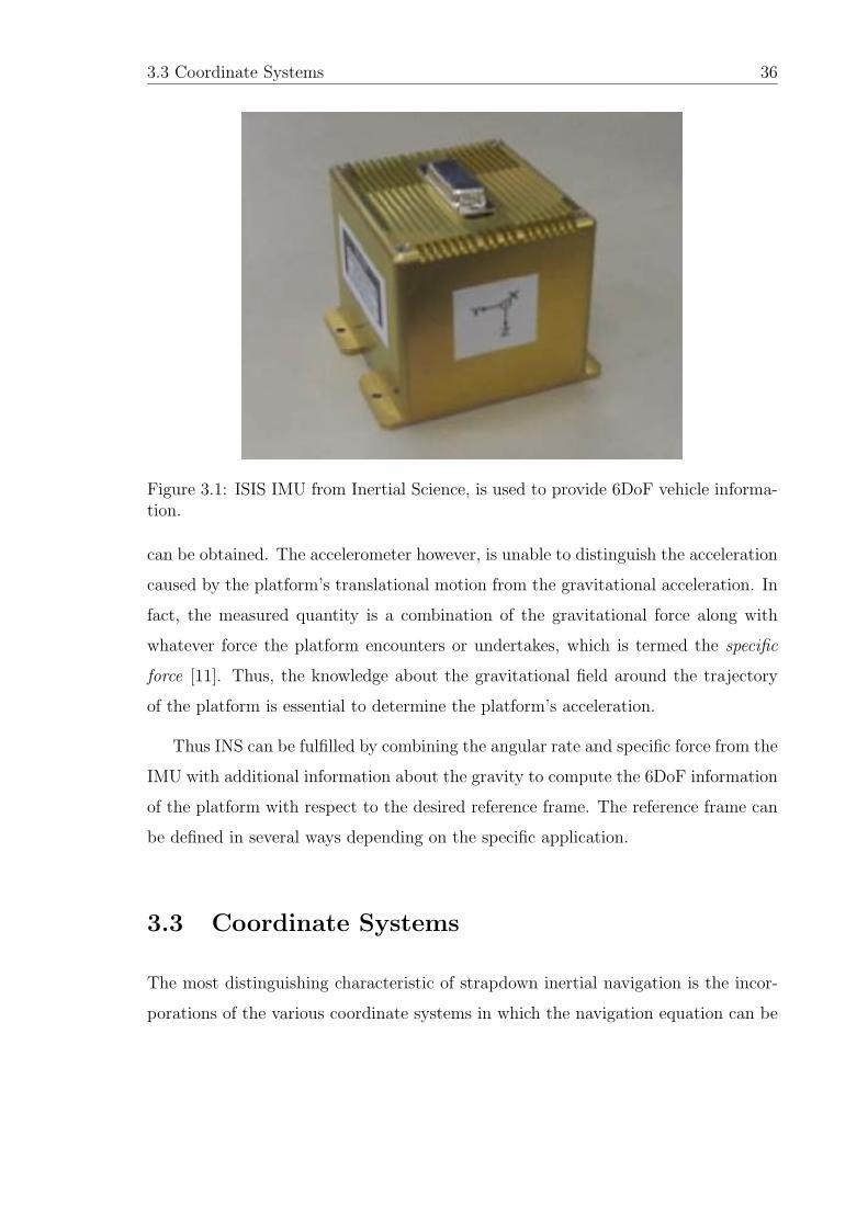
3.3 Coordinate Systems 36
Figure 3.1: ISIS IMU from Inertial Science, is used to provide 6DoF vehicle informa-tion.
can be obtained. The accelerometer however, is unable to distinguish the acceleration
caused by the platform’s translational motion from the gravitational acceleration. In
fact, the measured quantity is a combination of the gravitational force along with
whatever force the platform encounters or undertakes, which is termed the specific
force [11]. Thus, the knowledge about the gravitational field around the trajectory
of the platform is essential to determine the platform’s acceleration.
Thus INS can be fulfilled by combining the angular rate and specific force from the
IMU with additional information about the gravity to compute the 6DoF information
of the platform with respect to the desired reference frame. The reference frame can
be defined in several ways depending on the specific application.
3.3 Coordinate Systems
The most distinguishing characteristic of strapdown inertial navigation is the incor-
porations of the various coordinate systems in which the navigation equation can be
3.3 Coordinate Systems 37
formulated. Since the sensor measurements and navigation outputs are expressed in
different reference frames, a frame transformation is required. This section provides
the definitions of the coordinate frames used within this thesis.
3.3.1 Inertial Frame
An inertial frame is defined as a non-accelerating reference frame. The origin of this
coordinate system can be any point in the universe with three mutually orthogonal
axes.
Inertial sensors measure the specific force and rotation rate with respect to this
inertial frame in their sensitive axes. From the principle of general relativity, the
inertial and gravitational mass are equivalent and we cannot distinguish between
the gravitational acceleration and the corresponding acceleration of the platform.
Hence it is obviously necessary to completely specify the gravitational field around
the trajectory such that the platform’s acceleration can be extracted from the specific
force.
3.3.2 Earth-Centred Earth-Fixed Frame
The Earth-Centred Earth Fixed (ECEF) frame is defined with its origin fixed to
the centre of the Earth. The z-axis is coincident with the rotational axis of the
Earth and x-axis lies along Greenwich meridian. The y-axis is defined to complete
the right-handed coordinate system. This frame is not an inertial frame, since it
rotates along with the Earth with respect to the inertial space at approximately
7.292115×10⁻⁵rad/s.
In this frame, the platform’s position can be represented either in Cartesian coor-
dinate using x, y and z or a geodetic coordinate using latitude, longitude and height.
Both of these coordinate systems are useful in processing the GNSS data.
3.3 Coordinate Systems 38
3.3.3 Geographic Frame
The geographic frame is defined as a locally level frame with its origin at the platform’s
location. The z-axis (or down axis) is defined normal to the Earth’s reference ellipsoid,
which is an approximation to the gravitational equipotential surface, or geoid. The
x-axis (or north axis) points toward north and the y-axis (or east axis) points east on
the surface of the ellipsoid [11].
When the vehicle moves around the surface of the Earth, the geographic frame
moves as well. Hence the origin of this frame is successively redefined at the current
platform’s position projected onto the ellipsoidal surface. This means the frame
itself is dynamically changing and should be compensated properly according to the
position and velocity of the platform.
One interesting phenomenon about this frame is the Schuler oscillation observed in
the INS. Any tilt error makes the INS incorrectly interpret the accelerometer reading
from the gravitational acceleration and hence incorrectly reports that the vehicle
moves to one direction. As the position error increases, the INS tries to adjust its
attitude to the local tangent at the indicated position. Eventually, the frame will
be tilted significantly to one side and the accelerometer errors will begin to work in
the opposite direction and the position will be pulled back to the initial position and
so on. The oscillation frequency is determined by the curvature the surface (or the
radius of Earth) and the gravitational acceleration as in the case of a simple pendulum
problem [11].
3.3.4 Earth-Fixed Local-Tangent Frame
The geographic frame is typically implemented when large areas of travel are covered.
If the application is traversing within a small defined area, then an Earth-Fixed Local-
Tangent frame can be used. The origin is defined on a local reference point with its
x-axis pointing north, y-axis pointing east and the z-axis pointing down, making the
3.3 Coordinate Systems 39
frame a local tangent. Compared to the geographic frame, it is not moving, and to
the ECEF frame, it is locally tangent.
As for the metric representation, a coordinate system called the Universal Trans-
verse Mercator (UTM) is widely used which projects the geodetic position to a flat
metric map [34]. The coordinates in the north and east directions are referred to as
northing and easting. With this representation, the observations of the landmarks
from the on-board sensor can be easily represented in Cartesian coordinates. Al-
though the UTM is a world-wide system, there exist different degrees of distortions
depending on the regions so many countries use more refined models in their regions.
In Australia, the Map Grid Australia (MGA) is used which corresponds to the zone
numbers between 49 and 56 in the UTM. The conversion error between MGA and
WGS-84 is known to 1mm in any zone of Australia [33].
In this thesis, the INS equation is formulated using the Local- Tangent Earth-
Fixed frame with the MGA coordinate system. The GNSS solution expressed in
WGS-84 is firstly converted into the MGA coordinate, then fused in the filter.
3.3.5 Body Frame
The body frame is defined as a set of three orthogonal axes with its origin at the
centre of mass of the platform. The x-axis (or roll axis) points forward with respect
to the platform, the z-axis (or yaw axis) points down, and the y-axis (or pitch axis)
points out the right side which completes the right-handed coordinate system.
3.3.6 Sensor Frame
The sensor installed within the platform has its own sensor frame. The origin is at
the location of sensor and its axes are defined differently depending on the type of
sensor.
3.4 Inertial Navigation Equations 40
For an IMU, the origin is at the location of the IMU and the x, y and z-axes are
defined to the sensitive axes of the IMU. The IMU is typically installed such that its
sensitive axes are aligned to the body frame. If there are additional mission sensors,
such as vision or radar, then the observations are represented in their own sensor
frames. In this thesis, a vision camera is installed on the platform’s fuselage pointing
downward. The origin of the vision frame is at the location of the camera and the
x-axis points downward with respect to the body. The y-axis is identical to the pitch
axis of the body frame and the z-axis is chosen to complete a right-handed coordinate
system.
3.4 Inertial Navigation Equations
The inertial navigation equations is a set of differential equations which relates the
inertial quantities measured within the inertial frame to the navigation quantities
in the desired reference frame. Firstly, the attitude equation will be presented for
the purpose of the coordinate transformation. Then the velocity/position equations
will be presented. Depending on the applications, different reference frames may be
required which results in a different set of equations.
3.4.1 Attitude Equations
In this section, three different attitude algorithms in discrete time are provided: Euler
angle, Direction Cosine Matrix (DCM), and the quaternion algorithm. In addition,
the rotation vector algorithm is also provided to minimise the error of the finite
rotation during the attitude update interval [10].
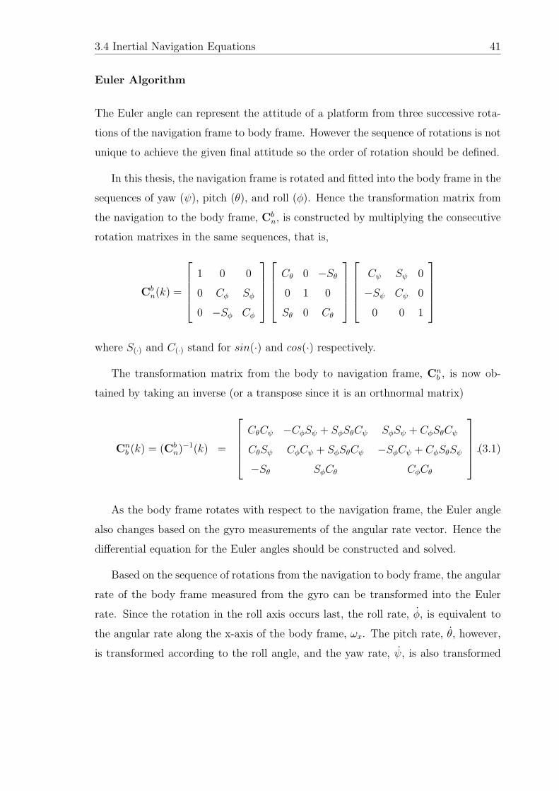
3.4 Inertial Navigation Equations 41
Euler Algorithm
The Euler angle can represent the attitude of a platform from three successive rota-
tions of the navigation frame to body frame. However the sequence of rotations is not
unique to achieve the given final attitude so the order of rotation should be defined.
In this thesis, the navigation frame is rotated and fitted into the body frame in the
sequences of yaw (ψ), pitch (θ), and roll (φ). Hence the transformation matrix from
the navigation to the body frame, Cbn, is constructed by multiplying the consecutive
rotation matrixes in the same sequences, that is,
Cbn(k) =
⎡⎢⎢⎢⎣
1 0 0
0 Cφ Sφ
0 −Sφ Cφ
⎤⎥⎥⎥⎦⎡⎢⎢⎢⎣Cθ 0 −Sθ0 1 0
Sθ 0 Cθ
⎤⎥⎥⎥⎦⎡⎢⎢⎢⎣
Cψ Sψ 0
−Sψ Cψ 0
0 0 1
⎤⎥⎥⎥⎦
where S(·) and C(·) stand for sin(·) and cos(·) respectively.
The transformation matrix from the body to navigation frame, Cnb , is now ob-
tained by taking an inverse (or a transpose since it is an orthnormal matrix)
Cnb (k) = (Cb
n)−1(k) =
⎡⎢⎢⎢⎣CθCψ −CφSψ + SφSθCψ SφSψ + CφSθCψ
CθSψ CφCψ + SφSθCψ −SφCψ + CφSθSψ
−Sθ SφCθ CφCθ
⎤⎥⎥⎥⎦ .(3.1)
As the body frame rotates with respect to the navigation frame, the Euler angle
also changes based on the gyro measurements of the angular rate vector. Hence the
differential equation for the Euler angles should be constructed and solved.
Based on the sequence of rotations from the navigation to body frame, the angular
rate of the body frame measured from the gyro can be transformed into the Euler
rate. Since the rotation in the roll axis occurs last, the roll rate, φ, is equivalent to
the angular rate along the x-axis of the body frame, ωx. The pitch rate, θ, however,
is transformed according to the roll angle, and the yaw rate, ψ, is also transformed
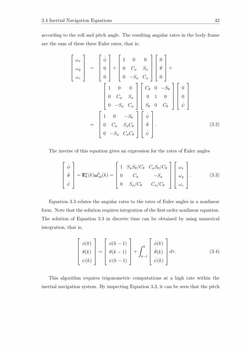
3.4 Inertial Navigation Equations 42
according to the roll and pitch angle. The resulting angular rates in the body frame
are the sum of these three Euler rates, that is:
⎡⎢⎢⎢⎣ωx
ωy
ωz
⎤⎥⎥⎥⎦ =
⎡⎢⎢⎢⎣φ
0
0
⎤⎥⎥⎥⎦+
⎡⎢⎢⎢⎣
1 0 0
0 Cφ Sφ
0 −Sφ Cφ
⎤⎥⎥⎥⎦⎡⎢⎢⎢⎣
0
θ
0
⎤⎥⎥⎥⎦+
⎡⎢⎢⎢⎣
1 0 0
0 Cφ Sφ
0 −Sφ Cφ
⎤⎥⎥⎥⎦⎡⎢⎢⎢⎣Cθ 0 −Sθ0 1 0
Sθ 0 Cθ
⎤⎥⎥⎥⎦⎡⎢⎢⎢⎣
0
0
ψ
⎤⎥⎥⎥⎦
=
⎡⎢⎢⎢⎣
1 0 −Sθ0 Cφ SφCθ
0 −Sφ CφCθ
⎤⎥⎥⎥⎦⎡⎢⎢⎢⎣φ
θ
ψ
⎤⎥⎥⎥⎦ . (3.2)
The inverse of this equation gives an expression for the rates of Euler angles
⎡⎢⎢⎢⎣φ
θ
ψ
⎤⎥⎥⎥⎦ = En
b (k)ωbnb(k) =
⎡⎢⎢⎢⎣
1 SφSθ/Cθ CφSθ/Cθ
0 Cφ −Sφ0 Sφ/Cθ Cφ/Cθ
⎤⎥⎥⎥⎦⎡⎢⎢⎢⎣ωx
ωy
ωz
⎤⎥⎥⎥⎦ . (3.3)
Equation 3.3 relates the angular rates to the rates of Euler angles in a nonlinear
form. Note that the solution requires integration of the first-order nonlinear equation.
The solution of Equation 3.3 in discrete time can be obtained by using numerical
integration, that is,
⎡⎢⎢⎢⎣φ(k)
θ(k)
ψ(k)
⎤⎥⎥⎥⎦ =
⎡⎢⎢⎢⎣φ(k − 1)
θ(k − 1)
ψ(k − 1)
⎤⎥⎥⎥⎦+
∫ k
k−1
⎡⎢⎢⎢⎣φ(k)
θ(k)
ψ(k)
⎤⎥⎥⎥⎦ dτ . (3.4)
This algorithm requires trigonometric computations at a high rate within the
inertial navigation system. By inspecting Equation 3.3, it can be seen that the pitch
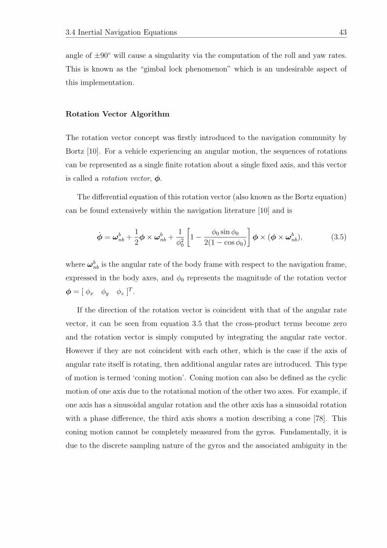
3.4 Inertial Navigation Equations 43
angle of ±90◦ will cause a singularity via the computation of the roll and yaw rates.
This is known as the “gimbal lock phenomenon” which is an undesirable aspect of
this implementation.
Rotation Vector Algorithm
The rotation vector concept was firstly introduced to the navigation community by
Bortz [10]. For a vehicle experiencing an angular motion, the sequences of rotations
can be represented as a single finite rotation about a single fixed axis, and this vector
is called a rotation vector, φ.
The differential equation of this rotation vector (also known as the Bortz equation)
can be found extensively within the navigation literature [10] and is
φ = ωbnb +1
2φ× ωbnb +
1
φ20
[1 − φ0 sinφ0
2(1 − cosφ0)
]φ× (φ× ωbnb), (3.5)
where ωbnb is the angular rate of the body frame with respect to the navigation frame,
expressed in the body axes, and φ0 represents the magnitude of the rotation vector
φ = [ φx φy φz ]T .
If the direction of the rotation vector is coincident with that of the angular rate
vector, it can be seen from equation 3.5 that the cross-product terms become zero
and the rotation vector is simply computed by integrating the angular rate vector.
However if they are not coincident with each other, which is the case if the axis of
angular rate itself is rotating, then additional angular rates are introduced. This type
of motion is termed ‘coning motion’. Coning motion can also be defined as the cyclic
motion of one axis due to the rotational motion of the other two axes. For example, if
one axis has a sinusoidal angular rotation and the other axis has a sinusoidal rotation
with a phase difference, the third axis shows a motion describing a cone [78]. This
coning motion cannot be completely measured from the gyros. Fundamentally, it is
due to the discrete sampling nature of the gyros and the associated ambiguity in the
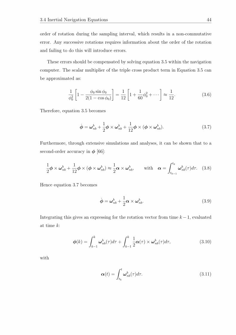
3.4 Inertial Navigation Equations 44
order of rotation during the sampling interval, which results in a non-commutative
error. Any successive rotations requires information about the order of the rotation
and failing to do this will introduce errors.
These errors should be compensated by solving equation 3.5 within the navigation
computer. The scalar multiplier of the triple cross product term in Equation 3.5 can
be approximated as:
1
φ20
[1 − φ0 sinφ0
2(1 − cosφ0)
]=
1
12
[1 +
1
60φ2
0 + · · ·]≈ 1
12. (3.6)
Therefore, equation 3.5 becomes
φ = ωbnb +1
2φ× ωbnb +
1
12φ× (φ× ωbnb). (3.7)
Furthermore, through extensive simulations and analyses, it can be shown that to a
second-order accuracy in φ [66]:
1
2φ× ωbnb +
1
12φ× (φ× ωbnb) ≈
1
2α× ωbnb, with α =
∫ tk
tk−1
ωbnb(τ)dτ. (3.8)
Hence equation 3.7 becomes
φ = ωbnb +1
2α× ωbnb. (3.9)
Integrating this gives an expressing for the rotation vector from time k−1, evaluated
at time k:
φ(k) =
∫ k
k−1
ωbnb(τ)dτ +
∫ k
k−1
1
2α(τ) × ωbnb(τ)dτ, (3.10)
with
α(t) =
∫ t
tk
ωbnb(τ)dτ. (3.11)
3.4 Inertial Navigation Equations 45
That is, the rotation vector can be constructed by integrating the angular rates
measured from the gyros, plus an additional correction term.
If the base motion is known beforehand, then Equation 3.10 can be further op-
timised by minimising the resulting errors. Typically a pure coning motion is as-
sumed and ωbnb(k) is approximated by truncating the series expansion [29, 30, 52].
The fourth-order algorithm presented in [48] is used in this thesis, which can be
written as
φ(k) = (θ1 + θ2 + θ3 + θ4) +54
105(θ1 × θ4) +
92
210(θ1 × θ3 + θ2 × θ4)
+214
315(θ1 × θ2 + θ2 × θ3 + θ3 × θ4) (3.12)
where θ1, θ1, θ3, and θ4 are the four gyro samples within the rotation vector update
interval, i.e, between k − 1 and k.
The attitude parameters, such as the DCM or the quaternion, can be computed
from this rotation vector, however, with much lower rates than the rotation vector
update rates (which is the gyro sample rates).
Direction Cosine Matrix Algorithm
The Direction Cosine Matrix (DCM), Cnb , is defined by the three direction cosine
vectors of the body axes with respect to the navigation frame.
The differential equation of Cnb can be obtained using small angle analyses [11]
and is
Cnb = Cn
b [ωbnb×], (3.13)
where [ωbnb×] is a skew-symmetric matrix for the angular rates of the body frame
3.4 Inertial Navigation Equations 46
with respect to the navigation frame and has a form:
[ωbnb×] =
⎡⎢⎢⎢⎣
0 −ωz ωy
ωz 0 −ωx−ωy ωx 0
⎤⎥⎥⎥⎦ . (3.14)
Equation 3.13 can be solved in the closed-form by applying an integration factor
method:
Cnb (k) = Cn
b (k − 1) exp
(∫ k
k−1
[ωbnb×]dτ
). (3.15)
The integration of the angular rates during the update interval with the coning cor-
rection becomes the rotation vector, φ, which is computed from Equation 3.12. Using
the skew-symmetric form of the rotation vector in Equation 3.15 gives
Cnb (k) = Cn
b (k − 1) exp ([φ×]). (3.16)
Expanding the exponential term into a series and using trigonometric functions gives
Cnb (k) = Cn
b (k − 1)
[I +
sinφ0
φ0
[φ(k)×] +1 − cosφ0
φ20
[φ(k)×]2], (3.17)
where φ0 is the magnitude of φ(k).
Equation 3.17 gives a representation of the DCM from the rotation vector during
the attitude update interval. In some cases (where there is only limited computational
power), the trigonometric coefficients may be expanded and truncated to a low order
polynomial [78]. It is also required to preserve the normality and/or orthogonality
of the DCM. The normalisation of the DCM can be performed by normalising each
column (or row) vector periodically.
The transformation of the vector quantity can now be performed by using this
3.4 Inertial Navigation Equations 47
DCM. The specific force vector in the navigation frame, fn(k), is
fn(k) = Cnb (k)f
b(k), (3.18)
where f b(k) is the specific force vector in the body axes which is the direct measure-
ment from the IMU.
Quaternion Algorithm
The quaternion is used to represent the attitude between the body and navigation
frame, and similar to the Euler and DCM approach, can be used to transform vector
quantities from one frame to another [66]. The quaternion is a four component vector:
q(k) = [ q0 q1 q2 q3 ]T . (3.19)
The quaternion differential equation provides a relation between the input angular
rates and the attitude quaternion and it has a form of
q =1
2q ⊗ ωbnb, (3.20)
where ⊗ represents the quaternion product between two quaternions as in [52], and
ωbnb = [ 0 ωbnb ]T is the quaternion form of the angular rate.
The quaternion equation can also be expressed in matrix form:
q =1
2[q⊗]ωbnb (3.21)
=1
2[ωbnb�]q, (3.22)
3.4 Inertial Navigation Equations 48
where [q⊗] and [ωbnb�] are the matrix forms of q and ωbnb, and are defined as
[q⊗] =
⎡⎢⎢⎢⎢⎢⎣
q0 −q1 −q2 −q3q1 q0 −q3 q2
q2 q3 q0 −q1q3 −q2 q1 q0
⎤⎥⎥⎥⎥⎥⎦ , [ωbnb�] =
⎡⎢⎢⎢⎢⎢⎣
0 −ωx −ωy −ωzωx 0 ωz −ωyωy −ωz 0 ωx
ωz ωy −ωx 0
⎤⎥⎥⎥⎥⎥⎦ (3.23)
and ωx, ωy, and ωz are the components of ωbnb. Note that two matrices have different
forms due to the non-commutativity in the quaternion product.
To solve Equation 3.22, a similar method to that used in the DCM can be applied.
That is, applying the integration factor method, using the rotation vector for the
angle integration during the update interval, and then expanding the exponential
term, gives
q(k) = exp
(1
2
∫ k
k−1
[ωbnb�]dτ
)q(k − 1), (3.24)
= exp
(1
2[φ�]
)q(k − 1), (3.25)
=
[cos
φ0
2[I] +
1
φ0
sinφ0
2[φ�]
]q(k − 1), (3.26)
where [I] is the matrix form of the unit quaternion, [ 1 0 0 0 ]T , and [φ�] is for
the quaternion of the rotation vector, φ = [ 0 φx φy φz ]T .
Two quaternions, I and φ, can be added up into a single quaternion �q(k), then
Equation 3.26 becomes,
q(k) = [�q(k)�]q(k − 1), (3.27)
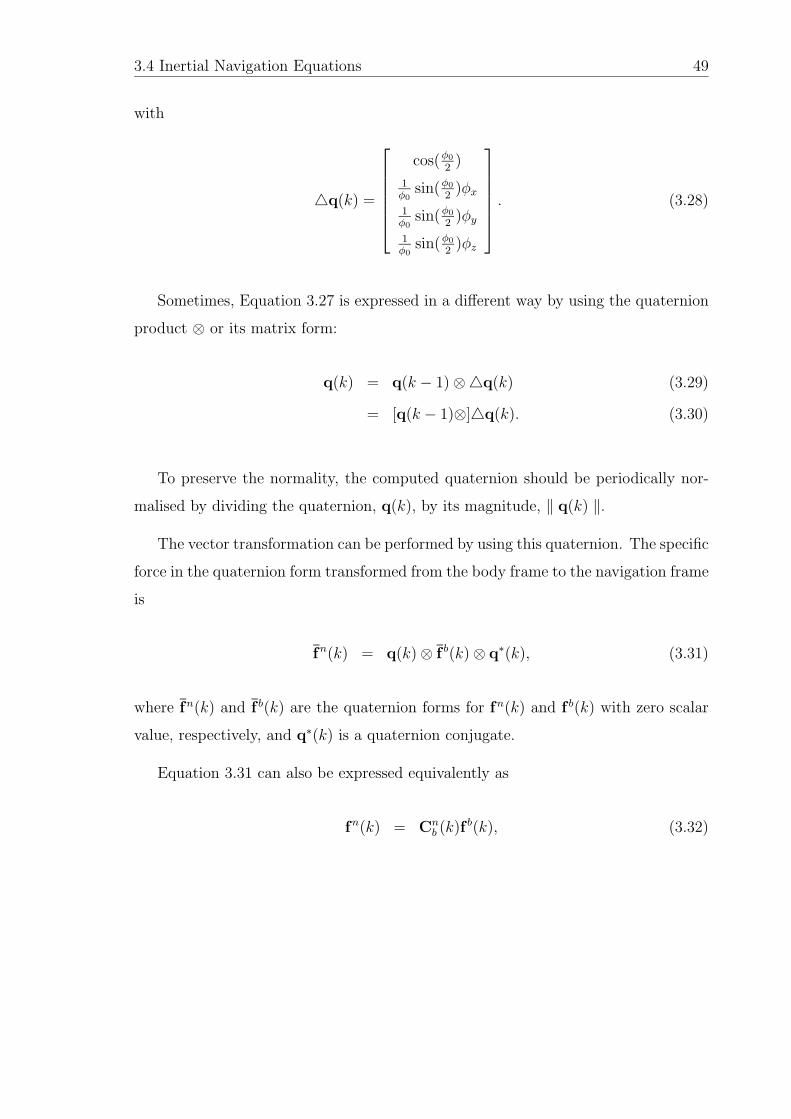
3.4 Inertial Navigation Equations 49
with
�q(k) =
⎡⎢⎢⎢⎢⎢⎣
cos(φ0
2)
1φ0
sin(φ0
2)φx
1φ0
sin(φ0
2)φy
1φ0
sin(φ0
2)φz
⎤⎥⎥⎥⎥⎥⎦ . (3.28)
Sometimes, Equation 3.27 is expressed in a different way by using the quaternion
product ⊗ or its matrix form:
q(k) = q(k − 1) ⊗�q(k) (3.29)
= [q(k − 1)⊗]�q(k). (3.30)
To preserve the normality, the computed quaternion should be periodically nor-
malised by dividing the quaternion, q(k), by its magnitude, ‖ q(k) ‖.
The vector transformation can be performed by using this quaternion. The specific
force in the quaternion form transformed from the body frame to the navigation frame
is
fn(k) = q(k) ⊗ f b(k) ⊗ q∗(k), (3.31)
where fn(k) and f b(k) are the quaternion forms for fn(k) and f b(k) with zero scalar
value, respectively, and q∗(k) is a quaternion conjugate.
Equation 3.31 can also be expressed equivalently as
fn(k) = Cnb (k)f
b(k), (3.32)
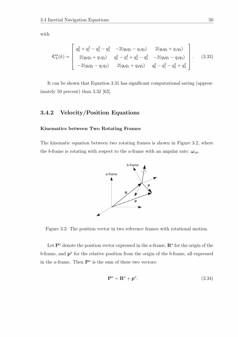
3.4 Inertial Navigation Equations 50
with
Cnb (k) =
⎡⎢⎢⎢⎣q20 + q2
1 − q22 − q2
3 −2(q0q3 − q1q2) 2(q0q2 + q1q3)
2(q0q3 + q1q2) q20 − q2
1 + q22 − q2
3 −2(q0q1 − q2q3)
−2(q0q2 − q1q3) 2(q0q1 + q2q3) q20 − q2
1 − q22 + q2
3
⎤⎥⎥⎥⎦ . (3.33)
It can be shown that Equation 3.31 has significant computational saving (approx-
imately 50 percent) than 3.32 [63].
3.4.2 Velocity/Position Equations
Kinematics between Two Rotating Frames
The kinematic equation between two rotating frames is shown in Figure 3.2, where
the b-frame is rotating with respect to the a-frame with an angular rate: ωab.
P
R
p
a-frame
b-frame
Figure 3.2: The position vector in two reference frames with rotational motion.
Let Pa denote the position vector expressed in the a-frame, Ra for the origin of the
b-frame, and pa for the relative position from the origin of the b-frame, all expressed
in the a-frame. Then Pa is the sum of these two vectors:
Pa = Ra + pa. (3.34)
3.4 Inertial Navigation Equations 51
By using the DCM Cab , the vector pa can be expressed in the b−frame:
Pa = Ra + Cabp
b. (3.35)
Differentiating this with respect to time, gives a velocity equation:
Pa = Ra + Cabp
b + Cab p
b. (3.36)
Applying the derivatives of the DCM, Cab = Ca
b [ωbab×], to the second term, gives
Pa = Ra + Cab
{[ωbab×]pb + pb
}. (3.37)
Differentiating this again and rearranging it, gives
Pa = Ra + Cab [ω
bab×]
{[ωbab×]pb + pb
}+ Ca
b
{ωbab×]pb + [ωab×]pb + pb
}= Ra + Ca
b
{2[ωbab×]pb + [ωbab×][ωbab×]pb + [ωbab×]pb + pb
}(3.38)
Note that Equation 3.38 is a general representation for the kinematics between
two rotating frames, which states that the acceleration in the non-rotating a−frame
is equal to the sum of the various accelerations in the b−frame. The first term in
Equation 3.38 is the acceleration of the frame itself, the second is known as the Coriolis
acceleration, the third is the centripetal acceleration, the fourth is the acceleration
due to the angular acceleration, and the last term is the acceleration in the rotating
frame.
Equation 3.38 forms the basis of inertial navigation. The only difference between
many navigation algorithms is the choice of the reference frame of interest.
3.4 Inertial Navigation Equations 52
Navigation in the Earth-Fixed Local-Tangent Frame
In navigating along with the Earth-Fixed Local-Tangent frame (or simply earth-fixed
navigation frame), the platform’s position and velocity are referenced with respect to
that axes.
Hence, by replacing the a-frame with the inertial frame (i-frame), and the b-frame
with the earth-fixed navigation frame (n-frame), Equation 3.38 becomes
Pi = Ri + Cin {2[ωnin×]pn + [ωnin×][ωnin×]pn + [ωnin×]pn + pn} . (3.39)
In the earth-fixed frame, the only rotational motion occurs from the Earth’s con-
stant rotation, hence the angular acceleration of this frame, [ωnin×], is zero, and the
linear acceleration, Ri, of this frame is also zero. By using these and rearranging in
terms of pn, gives
pn = Cni P
i − 2[ωnin×]pn − [ωnin×][ωnin×]pn. (3.40)
Now Cni P
i is the acceleration with respect to the inertial space, expressed in the
navigation axes. Since the IMU measures this quantity along with the gravitational
acceleration, this term can be expressed as the specific force in the navigation frame
with additional gravitational compensation term, that is,
Pn = Cni P
i = fn + gn(p). (3.41)
Substituting in Equation 3.40 and rearranging gives
pn = fn − 2[ωnin×]pn + {gn(p) − [ωnin×][ωnin×]pn} . (3.42)
Equation 3.42 describes the motion with respect to the navigation frame. The first
term is the specific force in the navigation frame which can be computed from the
3.4 Inertial Navigation Equations 53
body frame by using either the DCM in Equation 3.18 or the quaternion in Equation
3.31. The second term is the Coriolis term due to the rotational motion of the frame
(or the Earth equivalently). The Coriolis effect is proportional to the velocity and is
sometimes ignored, but it can be significant as is the case in this work. As an example,
the average speed of the platform used in this thesis is approximately 50m/s. In this
case, the maximum Coriolis acceleration becomes 0.74mg, which is not a negligible
value (The accelerometer used in this thesis has a bias specification of 1mg). The last
term is the effective local gravitational acceleration which is known as the ‘plumb-bob’
gravity.
Writing pn = vn and using an effective local gravity, Equation 3.42 becomes
vn = fn − 2[ωnin×]vn + gnl , (3.43)
with
gnl = gn(pn) − [ωnin×][ωnin×]pn. (3.44)
Now the velocity in the navigation frame in discrete time k, vn(k), can be com-
puted by integrating Equation 3.43 during the interval k − 1 to k:
vn(k) = vn(k − 1) +
∫ k
k−1
vn(τ)dτ. (3.45)
Finally, the position is computed by integrating the velocity:
pn(k) = pn(k − 1) +
∫ k
k−1
vn(τ)dτ. (3.46)
The choice of integration method is dependent on the applications. For airborne
applications, in which the performance is more demanding factor than the computa-
tional cost, a high order integration method is preferable, such as the Simpson’s rule
3.5 Error Analysis 54
or the fourth-order Runge-Kutta method.
3.5 Error Analysis
The objective of an inertial error analysis is to obtain a set of error equations or to
quantitatively evaluate the propagation and dynamics of the inertial errors. There has
been extensive research activities regarding INS error modelling, particularly within
a geographical frame [9, 24, 67]. In this thesis, the error model on the Earth-fixed
tangent frame is presented based on the work of [71].
3.5.1 Attitude Error Equations
The attitude error, δψn, is defined as the misalignment angle between the estimated
attitude and the true attitude. Hence the estimated attitude, Cnb , can be written as,
Cnb = (I − [δψn×])Cn
b (3.47)
where [δψn×] is a skew-symmetric matrix for the misalignment angle, and Cnb is the
true DCM.
Rearranging Equation 3.47 for [δψn×] gives:
[δψn×] = I − CnbC
nTb (3.48)
and differentiating this gives
[δψn×] = − ˙C
n
bCnTb − Cn
b CnTb . (3.49)
3.5 Error Analysis 55
The derivatives for the estimated and true DCM are, respectively,
˙Cn
b = Cnb [ω
bnb×], Cn
b = Cnb [ω
bnb×]. (3.50)
Substituting these into Equation 3.49 gives
[δψn×] = −(Cn
b [ωbnb×])CnT
b − Cnb (C
nb [ω
bnb×])T
= −Cnb ([ω
bnb×] − [ωbnb×])CnT
b (3.51)
where the skew-symmetric property is used, [ωbnb×]T = −[ωbnb×].
Writing [δωbnb×] = [ωbnb×] − [ωbnb×], then Equation 3.49 becomes
[δψn×] = −Cn
b [δωbnb×]CnT
b (3.52)
Substituting Equation 3.47 for the DCM, gives
[δψn×] = −(I − [δψn×])Cn
b [δωbnb×]CnT
b (3.53)
= −Cnb [δω
bnb×]CnT
b + [δψn×]Cnb [δω
bnb×]CnT
b . (3.54)
The product term of the two error matrixes [δψn×] and [δωbnb×] is insignificant and
assumed to be zero, thus
[δψn×] = −Cn
b [δωbnb×]CnT
b (3.55)
This is the similarity transformation of a matrix from the body to the navigation
frame, thus by using the transformed matrix notation, it can be written as
[δψn×] = −[δωnnb×] (3.56)
3.5 Error Analysis 56
In vector form, this becomes
δψn
= −δωnnb. (3.57)
Equation 3.57 is a general misalignment dynamic equation which states that the
rate of change in the misalignment angle is equal to the error in the angular rate of
the body frame with respect to the navigation frame. The same procedure can also
be performed for the attitude quaternion, which results in the same misalignment
equation in the geographic frame [67]. This equation is also valid regardless of the
choice of the specific navigation frame. In general, the angular rate of the body frame
with respect to the navigation frame, ωnnb, is the angular rate of the body frame with
respect to the inertial frame, ωnib, minus the angular rate of the navigation frame with
respect to the inertial frame, ωnin. Thus its error is
δωnnb = δωnib − δωnin. (3.58)
In the earth-fixed frame system, the navigation frame is fixed to the Earth and
undergoes the same constant rotational motion with the Earth. Thus its error can
be assumed to be zero, and Equation 3.57 becomes
δψn
= −δωnib = −Cnb δω
bib, (3.59)
From this equation, it can be seen that the misalignment error, in the earth-fixed
frame system, is only affected by the gyro errors.
3.5.2 Velocity/Position Error Equations
The velocity/position equations developed in the previous chapter are for the true
state without any errors in the attitude, accelerometers and gravitational model.
3.5 Error Analysis 57
However, the actual state is affected by these errors and hence a similar error analysis
is required.
The errors in the velocity/position are defined as the estimated quantity minus
the true quantity:
δvn � vn − vn (3.60)
δpn � pn − pn. (3.61)
Recall that the true velocity equation is
vn = Cnb fb − 2[ωnin×]vn + gnl , (3.62)
where the DCM is used to transform the specific force.
The estimated quantities contain errors,
˙vn
= Cnb fb − 2ωnin × vn + gnl . (3.63)
Substituting Equation 3.47 and applying the perturbation rule gives:
˙vn
= (I − [δψn×])Cnb (f
b + δf b) − 2(ωnin + δωnin) × (vn + δvn) + (gnl + δgnl ). (3.64)
The product of two error terms can be assumed to be zero. Expanding this and
subtracting it from Equation 3.62 gives an equation for the error:
δvn = −[δψn×]f b + Cnb δf
b − 2(δωnin × vn + ωnin × δvn) + δgnl . (3.65)
Since the navigation frame is fixed on the Earth, the error in the angular rate of the
navigation frame is zero. The gravity error is also assumed to be zero (If the error
contribution of this is significant to the overall performance, it should be included).
Using the vector product notation for [δψn×]f b = −f b× δψn and rearranging Equa-
3.5 Error Analysis 58
tion 3.65 gives,
δvn = −2ωnin × δvn + fn × δψn + Cnb δf
b, (3.66)
Thus the rate of change of the velocity error in the navigation frame, δvn, is equal to
the Coriolis acceleration caused by the velocity error, 2ωnin × δvn, together with the
acceleration caused by the misalignment, fn × δψn, and the errors associated with
the measurement of acceleration, δf b, transformed into the navigation frame.
If the velocity error is maintained within small value, the Coriolis term due to this
error can be ignored. For example, the velocity error in the real flight test, was
maintained below 0.5m/s. In that case, the maximum Coriolis acceleration is 7.44µg
which is an insignificant value compared to the sensor bias error of 1mg for the IMU
implemented in this thesis.
Since the velocity is defined by the derivative of the position, the position error
equation is simply obtained from the velocity error:
δpn = δvn. (3.67)
The INS error equation forms a basis to formulate the indirect filter in this thesis.
Due to the low-dynamic characteristics of the INS error, the prediction rate of the
filter can be lower than that of the IMU. Hence the system can be decoupled into the
high-speed INS module and the low-speed filter module. It also provides an insight of
the system behaviors such as the observability of the system, which is quite hard to
analysis for the nonlinear system directly. That is since the error equation becomes
piecewise constant, the observability of the nonlinear system can be investigated
analytically rather than numerically. It is this INS error equation which will be used
extensively, both in implementing the indirect SLAM in Chapter 4 and the GNSS
aided navigation in Chapter 5.
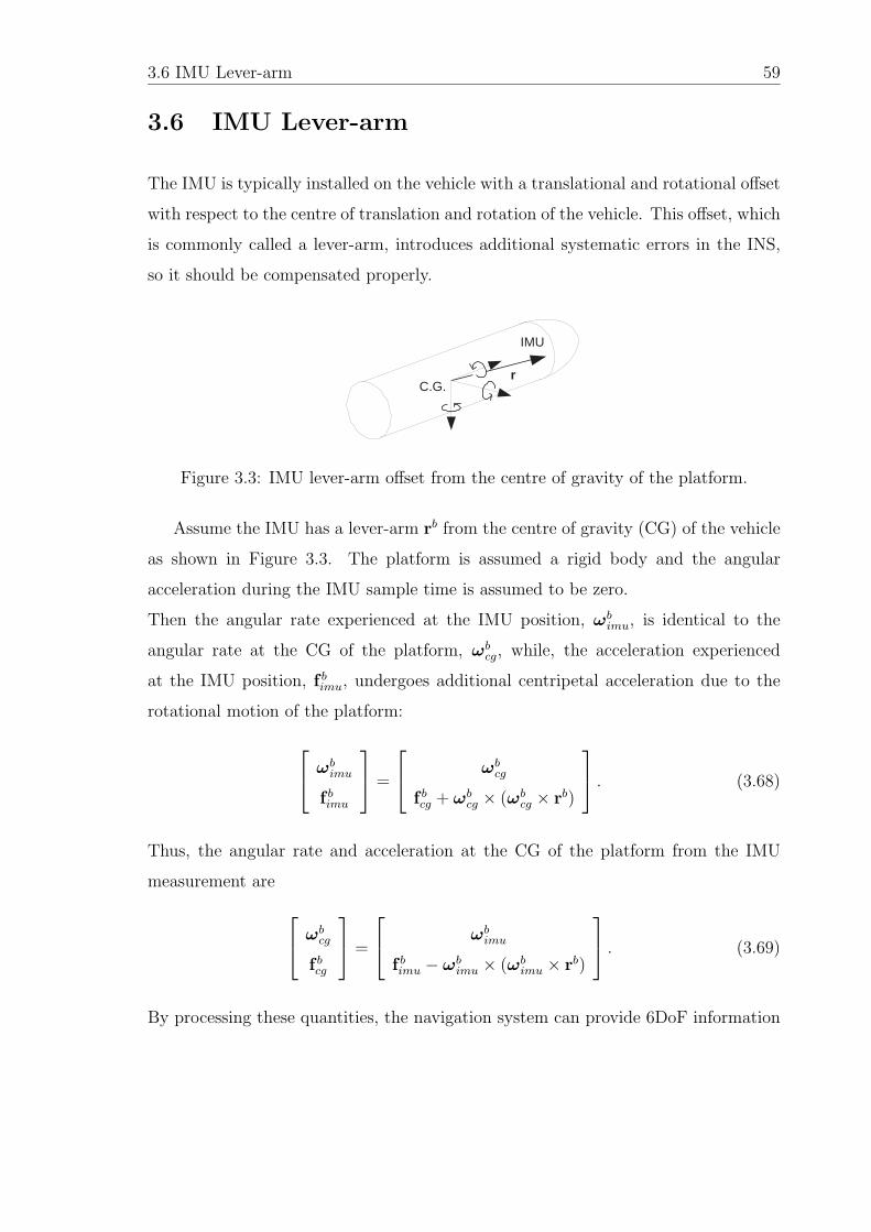
3.6 IMU Lever-arm 59
3.6 IMU Lever-arm
The IMU is typically installed on the vehicle with a translational and rotational offset
with respect to the centre of translation and rotation of the vehicle. This offset, which
is commonly called a lever-arm, introduces additional systematic errors in the INS,
so it should be compensated properly.
r
IMU
C.G.
Figure 3.3: IMU lever-arm offset from the centre of gravity of the platform.
Assume the IMU has a lever-arm rb from the centre of gravity (CG) of the vehicle
as shown in Figure 3.3. The platform is assumed a rigid body and the angular
acceleration during the IMU sample time is assumed to be zero.
Then the angular rate experienced at the IMU position, ωbimu, is identical to the
angular rate at the CG of the platform, ωbcg, while, the acceleration experienced
at the IMU position, f bimu, undergoes additional centripetal acceleration due to the
rotational motion of the platform:
⎡⎣ ωbimu
f bimu
⎤⎦ =
⎡⎣ ωbcg
f bcg + ωbcg × (ωbcg × rb)
⎤⎦ . (3.68)
Thus, the angular rate and acceleration at the CG of the platform from the IMU
measurement are
⎡⎣ ωbcg
f bcg
⎤⎦ =
⎡⎣ ωbimu
f bimu − ωbimu × (ωbimu × rb)
⎤⎦ . (3.69)
By processing these quantities, the navigation system can provide 6DoF information
3.7 Vibration 60
about the CG of the platform. This is important for autonomous operation of the
platform, since the flight control algorithm is based on the dynamics of the platform
at the CG.
As an example, in this thesis the IMU is installed with a lever-arm vector, [ 0.62m −0.06m 0.05m ]T in the body frame, and its sensitive axes are aligned to the body
frame. As the lever-arm vector has a large roll axis component, the pitch and yaw
motion can cause significant centripetal acceleration. The maximum angular rates
measured in the pitch and yaw axes from a typical flight were 0.611rad/s (or 35◦/s)
and 0.820rad/s (or 47◦/s), respectively. Then the maximum centripetal acceleration
computed from this information is -0.648m/s2 (or -65.3mg) along the x-axis. Clearly,
this should be compensated accordingly within the INS algorithm to provide a con-
sistent measurement to the flight controller which controls the vehicle with respect
to the CG of the vehicle.
3.7 Vibration
The vibration profile during flight imposes two issues on the inertial sensors: mini-
mum sampling frequency and coning errors. The minimum sampling rate of sensors
should meet the Nyquist sampling frequency criterion to measure the high frequency
vibration without aliasing. The vibration is also a common source for coning mo-
tion, which in turn introduces drifts in the attitude computation. This coning error
discussed in Section 3.4.1 will be analysed for the real vibration environment. If the
error contribution from the vibration exceeds the performance criterion it should be
compensated algorithmically or mechanically.
3.7.1 Sampling Frequency
The Nyquist sampling theorem provides a minimum sampling interval required to
avoid aliasing. It may be stated simply that the sampling frequency, fs, should be at
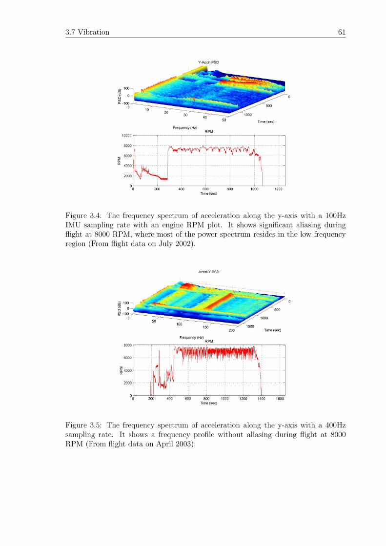
3.7 Vibration 61
Figure 3.4: The frequency spectrum of acceleration along the y-axis with a 100HzIMU sampling rate with an engine RPM plot. It shows significant aliasing duringflight at 8000 RPM, where most of the power spectrum resides in the low frequencyregion (From flight data on July 2002).
Figure 3.5: The frequency spectrum of acceleration along the y-axis with a 400Hzsampling rate. It shows a frequency profile without aliasing during flight at 8000RPM (From flight data on April 2003).
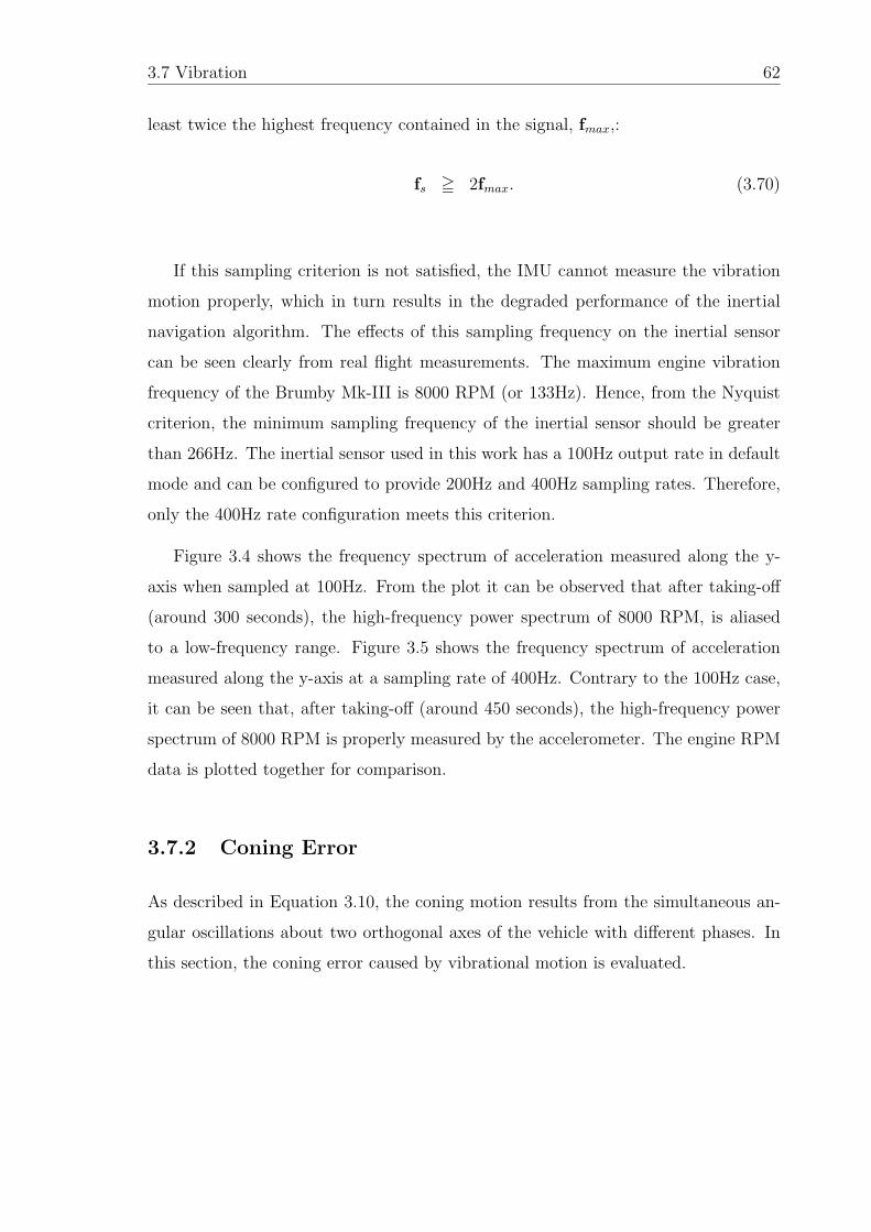
3.7 Vibration 62
least twice the highest frequency contained in the signal, fmax,:
fs � 2fmax. (3.70)
If this sampling criterion is not satisfied, the IMU cannot measure the vibration
motion properly, which in turn results in the degraded performance of the inertial
navigation algorithm. The effects of this sampling frequency on the inertial sensor
can be seen clearly from real flight measurements. The maximum engine vibration
frequency of the Brumby Mk-III is 8000 RPM (or 133Hz). Hence, from the Nyquist
criterion, the minimum sampling frequency of the inertial sensor should be greater
than 266Hz. The inertial sensor used in this work has a 100Hz output rate in default
mode and can be configured to provide 200Hz and 400Hz sampling rates. Therefore,
only the 400Hz rate configuration meets this criterion.
Figure 3.4 shows the frequency spectrum of acceleration measured along the y-
axis when sampled at 100Hz. From the plot it can be observed that after taking-off
(around 300 seconds), the high-frequency power spectrum of 8000 RPM, is aliased
to a low-frequency range. Figure 3.5 shows the frequency spectrum of acceleration
measured along the y-axis at a sampling rate of 400Hz. Contrary to the 100Hz case,
it can be seen that, after taking-off (around 450 seconds), the high-frequency power
spectrum of 8000 RPM is properly measured by the accelerometer. The engine RPM
data is plotted together for comparison.
3.7.2 Coning Error
As described in Equation 3.10, the coning motion results from the simultaneous an-
gular oscillations about two orthogonal axes of the vehicle with different phases. In
this section, the coning error caused by vibrational motion is evaluated.
3.7 Vibration 63
Recall the coning correction term in Equation 3.10 is
δα(t) =1
2
∫ t
tk−1
α(τ) × ω(τ)dτ, with α(t) =
∫ t
tk−1
ω(τ)dτ. (3.71)
As this equation is for the general angular motion, a sinusoidal angular motion with
frequency ω0 is used:
ω(t) =
⎡⎢⎢⎢⎣
ax cos(ω0t)
ay cos(ω0t+ φ1)
az cos(ω0t+ φ2)
⎤⎥⎥⎥⎦ (3.72)
where ax, ay, az are the amplitudes of angular rate in each axis, and φ1, φ2 are the
phase offsets.
Integrating Equation 3.72 and substituting into Equation 3.71 gives
δα(k) =1
2ω0
∫ tk
tk−1
⎡⎢⎢⎢⎣
ax[sin(ω0τ) − sin(ω0tk)]
ay[sin(ω0τ + φ1) − sin(ω0tk + φ1)]
az[sin(ω0τ + φ2) − sin(ω0tk + φ2)]
⎤⎥⎥⎥⎦×
⎡⎢⎢⎢⎣
ax cos(ω0τ)
ay cos(ω0τ + φ1)
az cos(ω0τ + φ2)
⎤⎥⎥⎥⎦ dτ
Performing this integral over the update interval �t, applying trigonometric manip-
ulations, and dividing by �t gives the average coning drift rate in analytic form:
δαav =1
2ω0
⎡⎢⎢⎢⎣ayaz sin(φ2 − φ1)
(1 − sin(ω0�t)
ω0�t
)−azax sin(φ2)
(1 − sin(ω0�t)
ω0�t
)axay sin(φ1)
(1 − sin(ω0�t)
ω0�t
)⎤⎥⎥⎥⎦ . (3.73)
Equation 3.73 describes the error contributions to the coning drift rate:
• The coning drift is proportional to the amplitude of each of the angular rates
measured from the gyros.
• As the attitude update interval decreases, the function(1 − sin(ω0�t)
ω0�t
)decreases
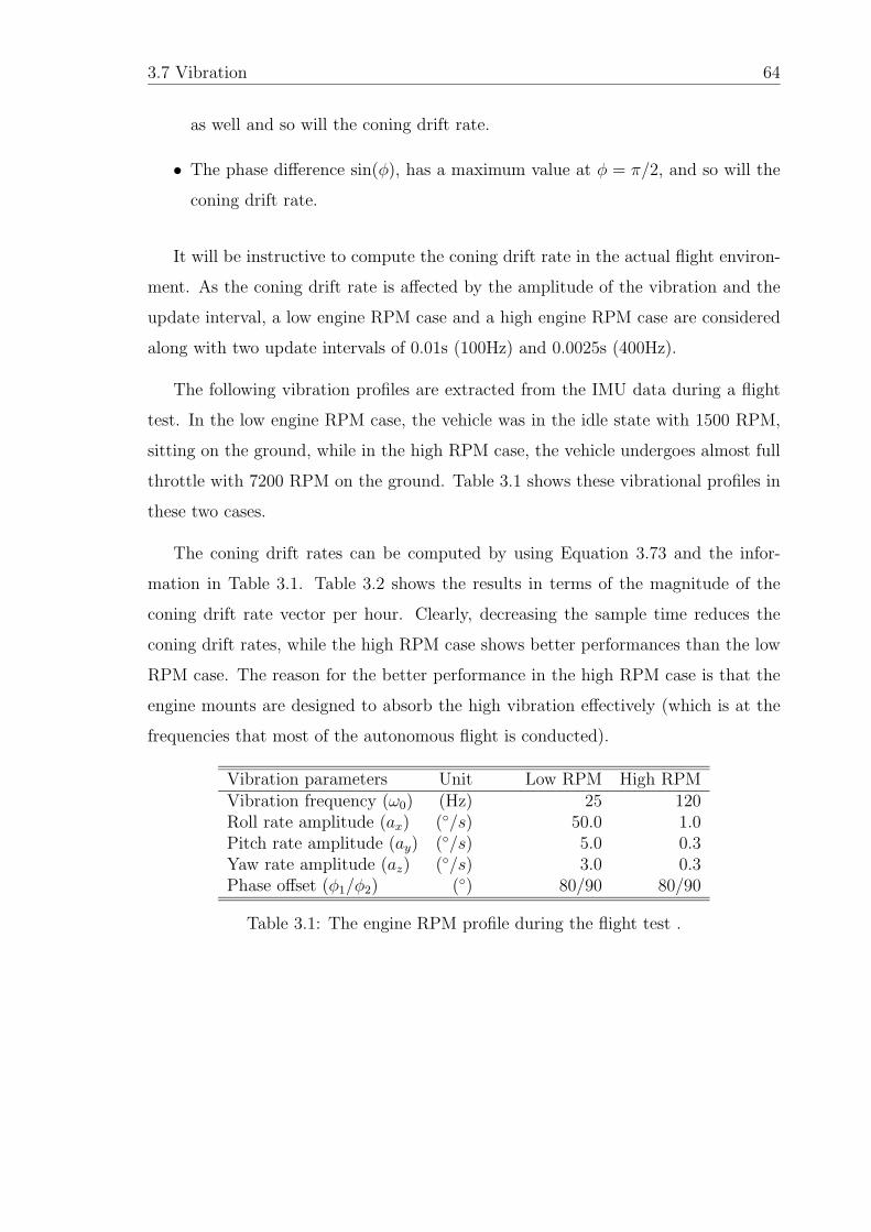
3.7 Vibration 64
as well and so will the coning drift rate.
• The phase difference sin(φ), has a maximum value at φ = π/2, and so will the
coning drift rate.
It will be instructive to compute the coning drift rate in the actual flight environ-
ment. As the coning drift rate is affected by the amplitude of the vibration and the
update interval, a low engine RPM case and a high engine RPM case are considered
along with two update intervals of 0.01s (100Hz) and 0.0025s (400Hz).
The following vibration profiles are extracted from the IMU data during a flight
test. In the low engine RPM case, the vehicle was in the idle state with 1500 RPM,
sitting on the ground, while in the high RPM case, the vehicle undergoes almost full
throttle with 7200 RPM on the ground. Table 3.1 shows these vibrational profiles in
these two cases.
The coning drift rates can be computed by using Equation 3.73 and the infor-
mation in Table 3.1. Table 3.2 shows the results in terms of the magnitude of the
coning drift rate vector per hour. Clearly, decreasing the sample time reduces the
coning drift rates, while the high RPM case shows better performances than the low
RPM case. The reason for the better performance in the high RPM case is that the
engine mounts are designed to absorb the high vibration effectively (which is at the
frequencies that most of the autonomous flight is conducted).
Vibration parameters Unit Low RPM High RPMVibration frequency (ω0) (Hz) 25 120Roll rate amplitude (ax) (◦/s) 50.0 1.0Pitch rate amplitude (ay) (◦/s) 5.0 0.3Yaw rate amplitude (az) (◦/s) 3.0 0.3Phase offset (φ1/φ2) (◦) 80/90 80/90
Table 3.1: The engine RPM profile during the flight test .
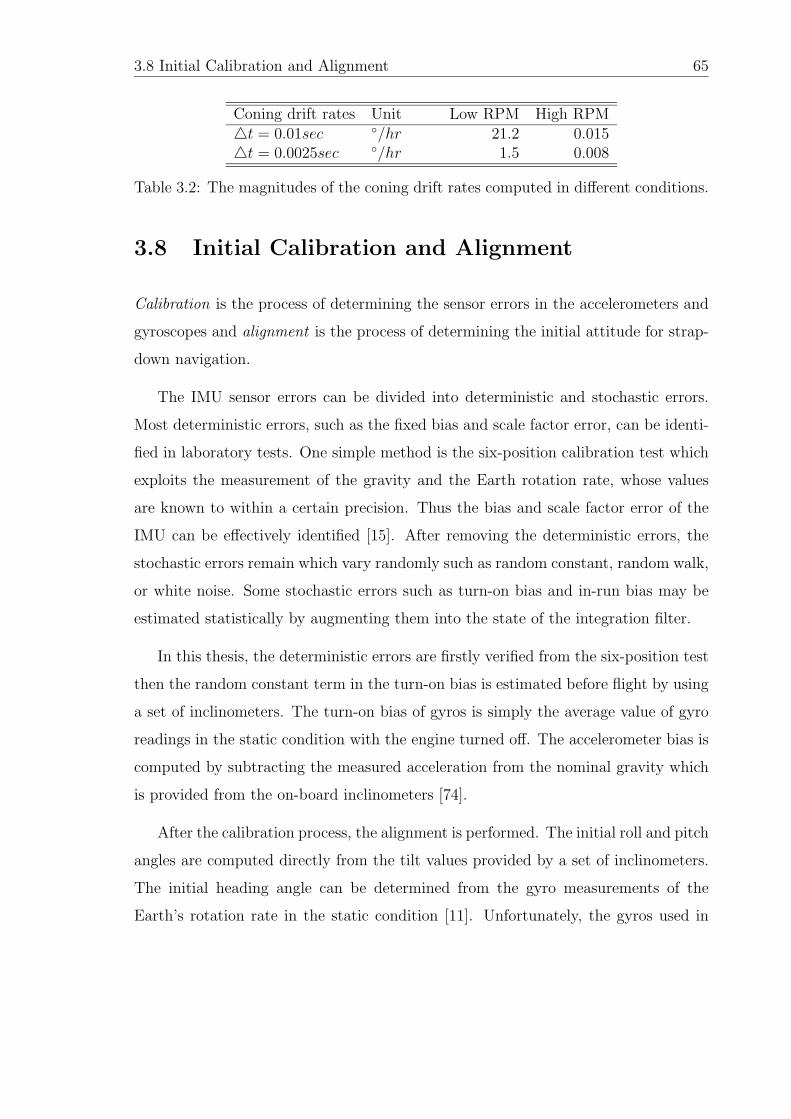
3.8 Initial Calibration and Alignment 65
Coning drift rates Unit Low RPM High RPM�t = 0.01sec ◦/hr 21.2 0.015�t = 0.0025sec ◦/hr 1.5 0.008
Table 3.2: The magnitudes of the coning drift rates computed in different conditions.
3.8 Initial Calibration and Alignment
Calibration is the process of determining the sensor errors in the accelerometers and
gyroscopes and alignment is the process of determining the initial attitude for strap-
down navigation.
The IMU sensor errors can be divided into deterministic and stochastic errors.
Most deterministic errors, such as the fixed bias and scale factor error, can be identi-
fied in laboratory tests. One simple method is the six-position calibration test which
exploits the measurement of the gravity and the Earth rotation rate, whose values
are known to within a certain precision. Thus the bias and scale factor error of the
IMU can be effectively identified [15]. After removing the deterministic errors, the
stochastic errors remain which vary randomly such as random constant, random walk,
or white noise. Some stochastic errors such as turn-on bias and in-run bias may be
estimated statistically by augmenting them into the state of the integration filter.
In this thesis, the deterministic errors are firstly verified from the six-position test
then the random constant term in the turn-on bias is estimated before flight by using
a set of inclinometers. The turn-on bias of gyros is simply the average value of gyro
readings in the static condition with the engine turned off. The accelerometer bias is
computed by subtracting the measured acceleration from the nominal gravity which
is provided from the on-board inclinometers [74].
After the calibration process, the alignment is performed. The initial roll and pitch
angles are computed directly from the tilt values provided by a set of inclinometers.
The initial heading angle can be determined from the gyro measurements of the
Earth’s rotation rate in the static condition [11]. Unfortunately, the gyros used in
3.9 Summary 66
this thesis are of low grade and do not have enough resolution to detect the Earth’s
rotation rate. The resolution of these gyros, or their minimum detectable angular
rate, in the roll (and likewise with pitch) and yaw axes are 0.0167 ◦/s and 0.0067 ◦/s
respectively. However the magnitude of the Earth’s rotation rate is approximately
15 ◦/h (or 0.0042 ◦/s). As a result, the measurement of the Earth’s rotation rate
for short durations of time does not provide sufficient information to compute the
heading orientation of the platform. Hence the autonomous determination of heading
cannot be implemented, and so the initial heading angle is provided by either an
operator or through the use of a multi-antenna GPS attitude system.
3.9 Summary
This chapter has provided the strapdown inertial navigation algorithms which are
used in the airborne navigation algorithms throughout this thesis (and for any other
6DoF motion).
In formulating the inertial navigation equations, the Earth-Fixed Local-Tangent
frame was used as the reference frame. The attitude algorithms were presented by
using the Euler angle, DCM, and quaternion in discrete form. To reduce the coning
error, the rotation vector algorithm was used during the attitude update interval.
The velocity/position algorithms were then formulated from the general kinematic
equations between rotating frames.
The error behaviours of the inertial algorithms were investigated by performing an
error analysis. The error equations will form the basis of the SLAM and GNSS aided
navigation system with the indirect filter structure. The effects from the IMU lever-
arm, sampling frequency and coning error were also analysed and discussed for the
real flight environments. Finally the initialisation techniques for inertial navigation
were discussed.
Chapter 4
Airborne 6DoF SLAM Navigation
4.1 Introduction
Simultaneous Localisation and Mapping (SLAM) is a method for building a navigation
map of an environment from a moving vehicle while simultaneously estimating the
location and trajectory of this platform. This chapter describes the development of
the SLAM algorithm for a 6DoF platform navigating within a 3D environment. Three
SLAM algorithms are developed in this chapter:
• The direct 6DoF SLAM algorithm using the total state and the nonlinear vehicle
and observation model.
• The indirect 6DoF SLAM algorithm using the error state and the linearised
error dynamic model of the vehicle and map.
• The 6DoF SLAM algorithm for multi-vehicle localisation using the 6DoF SLAM
as its local filter and exchanging the 3D map information over the information
network in Decentralised Data Fusion (DDF) framework.
While the 2D platform SLAM algorithm in land vehicles has received considerable
attention in the past few years [14, 19, 26, 49, 77], the SLAM problem in airborne
applications has only recently been addressed [35] and this chapter presents the first
4.2 6DoF SLAM Algorithm 68
developments of SLAM in the full 6DoF UAV platform which runs in real-time and
uses an IMU as part of a complete navigation system.
Furthermore, since the SLAM implementation presented in this thesis makes use
of an inertial navigation system as the driver for the process model, no vehicle model
is required, thus providing a navigation solution which is totally independent of the
vehicle implemented.
In addition, although the DDF SLAM problem in the multi-vehicle platform was
first formulated in [58], it was based on a simple tricycle model used as a land vehicle.
This chapter provides a truly DDF multi-vehicle SLAM algorithm for the 6DoF UAV
platforms in an information filter framework. The resulting structure is relevant for
any vehicle whether navigating in a 2D or 3D environment, and whether it undergoes
3DoF or 6DoF motion.
In this chapter the mathematical development of 6DoF SLAM is presented, with
results provided in Chapter 7.
4.2 6DoF SLAM Algorithm
The mathematical framework of the airborne SLAM algorithm is based on an estima-
tion process which, when given a kinematic/dynamic model of the UAV and relative
observations between the UAV and landmarks, estimates the structure of the map
and the UAV’s position, velocity and attitude within that map [41, 43].
The EKF is used as a state estimator for the vehicle and landmark position. The
structure of the algorithm is illustrated in Figure 4.1. The state and its covariance are
predicted using the control input which typically runs at high-frequency to track the
maneuvering aircraft. Whenever a landmark is observed a data association process is
conducted which checks to see if the landmark has been previously observed. If the
landmark has been previously registered in the filter, the observation is used to update
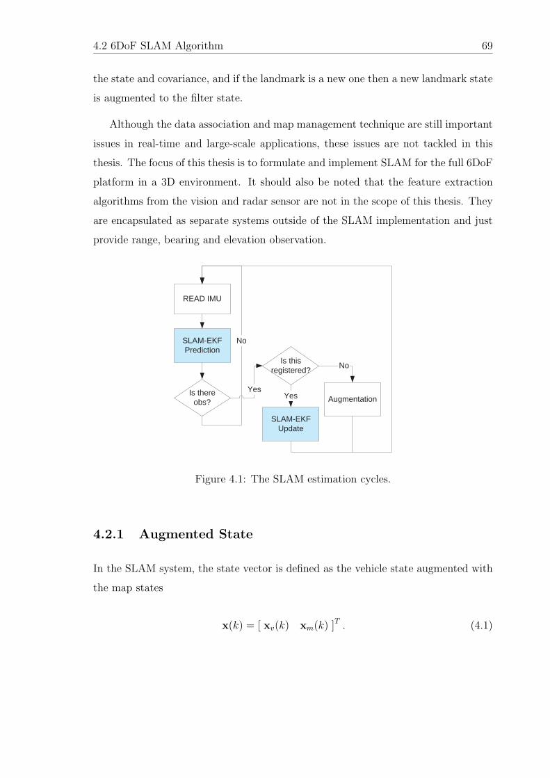
4.2 6DoF SLAM Algorithm 69
the state and covariance, and if the landmark is a new one then a new landmark state
is augmented to the filter state.
Although the data association and map management technique are still important
issues in real-time and large-scale applications, these issues are not tackled in this
thesis. The focus of this thesis is to formulate and implement SLAM for the full 6DoF
platform in a 3D environment. It should also be noted that the feature extraction
algorithms from the vision and radar sensor are not in the scope of this thesis. They
are encapsulated as separate systems outside of the SLAM implementation and just
provide range, bearing and elevation observation.
READ IMU
SLAM-EKFPrediction
Is thereobs? Augmentation
Is thisregistered?
SLAM-EKFUpdate
Yes
No
Yes
No
Figure 4.1: The SLAM estimation cycles.
4.2.1 Augmented State
In the SLAM system, the state vector is defined as the vehicle state augmented with
the map states
x(k) = [ xv(k) xm(k) ]T . (4.1)
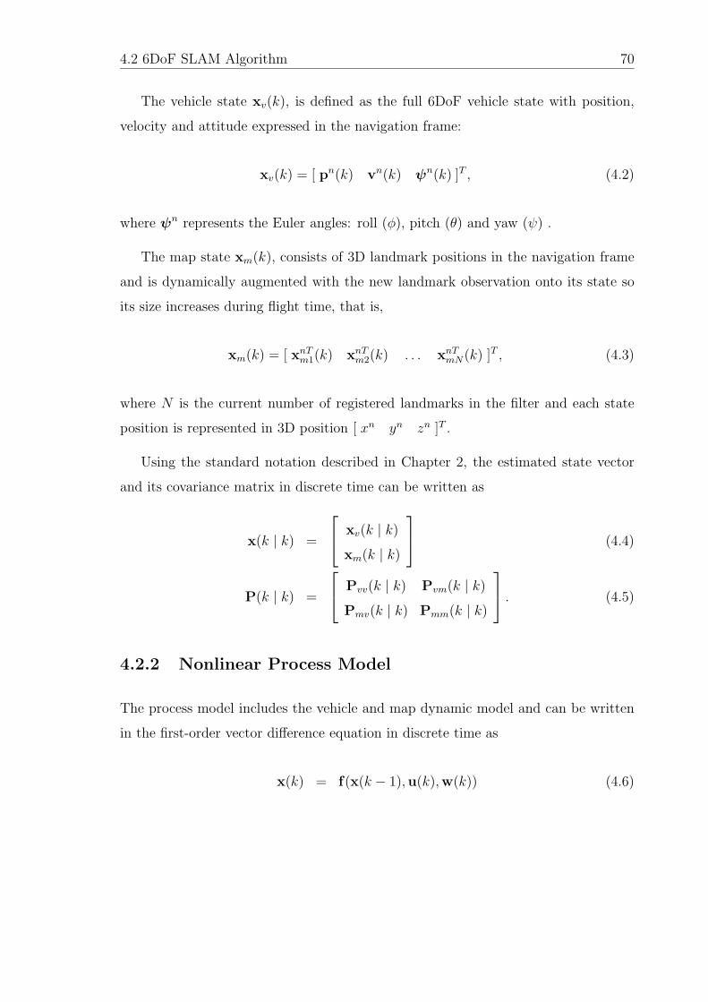
4.2 6DoF SLAM Algorithm 70
The vehicle state xv(k), is defined as the full 6DoF vehicle state with position,
velocity and attitude expressed in the navigation frame:
xv(k) = [ pn(k) vn(k) ψn(k) ]T , (4.2)
where ψn represents the Euler angles: roll (φ), pitch (θ) and yaw (ψ) .
The map state xm(k), consists of 3D landmark positions in the navigation frame
and is dynamically augmented with the new landmark observation onto its state so
its size increases during flight time, that is,
xm(k) = [ xnTm1(k) xnTm2(k) . . . xnTmN(k) ]T , (4.3)
where N is the current number of registered landmarks in the filter and each state
position is represented in 3D position [ xn yn zn ]T .
Using the standard notation described in Chapter 2, the estimated state vector
and its covariance matrix in discrete time can be written as
x(k | k) =
⎡⎣ xv(k | k)
xm(k | k)
⎤⎦ (4.4)
P(k | k) =
⎡⎣ Pvv(k | k) Pvm(k | k)
Pmv(k | k) Pmm(k | k)
⎤⎦ . (4.5)
4.2.2 Nonlinear Process Model
The process model includes the vehicle and map dynamic model and can be written
in the first-order vector difference equation in discrete time as
x(k) = f(x(k − 1),u(k),w(k)) (4.6)
4.2 6DoF SLAM Algorithm 71
where f(·, ·, ·) is a non-linear state transition function at time k which forms the
current vehicle and map state, x(k), from the previous state, x(k − 1), the current
control input, u(k), and the process noise, w(k).
The state transition model can be partitioned into the vehicle state dynamic model
and the map state dynamic model:
⎡⎣ xv(k)
xm(k)
⎤⎦ =
⎡⎣ fv(xv(k − 1),u(k),wv(k))
fm(xm(k − 1),wm(k))]
⎤⎦ . (4.7)
The process noise, wv(k), in Equation 4.7 is modelled as a zero mean Gaussian noise
with the noise strength of sensor errors:
E[wv(k)] = 0
E[wv(k)wv(k)T ] = Q(k) =
⎡⎣ σ2
fb 0
0 σ2ωb
⎤⎦ . (4.8)
The nonlinear vehicle model is a strapdown INS algorithm which computes the
position, velocity and attitude of the aircraft from the inertial measurement inputs.
In the Earth-Fixed Local-Tangent frame formulation with Euler angles as its attitude
parameters, the vehicle model becomes
⎡⎢⎢⎢⎣
pn(k)
vn(k)
ψn(k)
⎤⎥⎥⎥⎦ =
⎡⎢⎢⎢⎣
pn(k − 1) + vn(k − 1)�tvn(k − 1) + {Cn
b (k − 1)[f b(k) + δf b(k)] + gn}�tψn(k − 1) + En
b (k − 1)[ωb(k) + δωb(k)]�t
⎤⎥⎥⎥⎦+
⎡⎢⎢⎢⎣
wpn(k)
wvn(k)
wψn(k)
⎤⎥⎥⎥⎦(4.9)
where pn(k) and vn(k) are the position and velocity in the earth-fixed frame, and
ψn(k) is the Euler angle. f b(k) and ωb(k) is the acceleration and rotation rates
measured in the body frame, and Cnb is the DCM defined in Equation 3.1 and En
b is
the matrix that transforms the rotation rate in the body frame to the Euler angle
rate as defined in Equation 3.3.
4.2 6DoF SLAM Algorithm 72
A stationary landmark dynamic model is used with zero input disturbance. Hence
the state transition equation for the ith landmark in Equation 4.9 simply becomes
xnmi(k) = xnmi(k − 1). (4.10)
The Jacobian ∇fx(k) of the nonlinear vehicle model with respect to the vehicle
state can be computed as,
∇fx(k) =
⎡⎢⎢⎢⎣
∂pn(k)∂pn(k−1)
∂pn(k)∂vn(k−1)
∂pn(k)∂ψn(k−1)
∂vn(k)∂pn(k−1)
∂vn(k)∂vn(k−1)
∂vn(k)∂ψn(k−1)
∂ψn(k)∂pn(k−1)
∂ψn(k)∂vn(k−1)
∂ψn(k)∂ψn(k−1)
⎤⎥⎥⎥⎦ (4.11)
=
⎡⎢⎢⎢⎣
I �tI 0
0 I �t∂(Cnb (k−1)fb(k))
∂ψn(k−1)
0 0 I + �t∂(Enb (k−1)ωb(k))
∂ψn(k−1)
⎤⎥⎥⎥⎦ , (4.12)
where the sub-matrix can also be computed by taking Jacobians of Cnb and En
b with
respect to the Euler angles (ρ, ψ, θ). The Jacobian of Cnb (k − 1)f b(k) are computed
by,
∂(Cnb (k − 1)f b(k))
∂ψn(k − 1)=
⎡⎢⎢⎢⎣
∂fnn (k)
∂φ(k−1)∂fn
n (k)∂θ(k−1)
∂fnn (k)
∂ψ(k−1)
∂fne (k)
∂φ(k−1)∂fn
e (k)∂θ(k−1)
∂fne (k)
∂ψ(k−1)
∂fnd (k)
∂φ(k−1)
∂fnd (k)
∂θ(k−1)
∂fnd (k)
∂ψ(k−1)
⎤⎥⎥⎥⎦ (4.13)
where fn(k) = [fnn fne fnd ]T is used and the elements of the Jacobian can be com-
4.2 6DoF SLAM Algorithm 73
puted by using Equation 3.1:
∂fnn∂φ
= f by(SφSψ + CφSθCψ) + f bz (CφSψ − SφSθCψ)
∂fnn∂θ
= −f bxSθCψ + f bySφCθCψ + f bzCφCθCψ
∂fnn∂ψ
= −f bxCθSψ − f by(CφCψ + SφSθSψ) + f bz [SφCψ − CφSθSψ]
∂fne∂φ
= −f by(SφCψ − CφSθSψ) − f bz (CφCψ + SφSθSψ)
∂fne∂θ
= −f bxSθSψ + f bySφCθSψ + f bzCφCθSψ
∂fne∂ψ
= f bxCθCψ + f by(−CφSψ + SφSθCψ) + f bz (SφSψ + CφSθCψ)
∂fnd∂φ
= f byCφ − f bzSφCθ
∂fnd∂θ
= −f bxCθ − f bySφSθ − f bzCφSθ
∂fnd∂ψ
= 0
The Jacobian of Enb (k − 1)ωb(k) in Equation 4.12 is computed by
∂Enb (k − 1)ωb(k)
∂ψn(k − 1)=
⎡⎢⎢⎢⎣
∂φ(k)∂φ(k−1)
∂φ(k)∂θ(k−1)
∂φ(k)∂ψ(k−1)
∂θ(k)∂φ(k−1)
∂θ(k)∂θ(k−1)
∂θ(k)∂ψ(k−1)
∂ψ(k)∂φ(k−1)
∂ψ(k)∂θ(k−1)
∂ψ(k)∂ψ(k−1)
⎤⎥⎥⎥⎦ (4.14)
where the elements of the matrix are computed as
∂φ
∂φ=
SθCθ
(ωbyCφ − ωbzSφ),∂φ
∂θ=
1
C2θ
(ωbySφ + ωbzCφ),∂φ
∂ψ= 0
∂θ
∂φ= −ωbySφ − ωbzCφ,
∂θ
∂θ= 0,
∂θ
∂ψ= 0
∂ψ
∂φ=
1
Cθ(ωbyCφ − ωbzSφ),
∂ψ
∂θ=SθC2θ
(ωbySφ + ωbzCφ),∂ψ
∂ψ= 0
The Jacobian ∇fw(k) of the nonlinear process model is computed with respect to
4.2 6DoF SLAM Algorithm 74
the current sensor inputs, that is the specific force and angular rate:
∇fw(k) =
⎡⎢⎢⎢⎣
∂pn(k)∂fb(k)
∂pn(k)∂ωb(k)
∂vn(k)∂fb(k)
∂vn(k)∂ωb(k)
∂ψn(k)∂fb(k)
∂ψn(k)∂ωb(k)
⎤⎥⎥⎥⎦ (4.15)
=
⎡⎢⎢⎢⎣
0 0√�tCn
b (k − 1) 0
0√�tEn
b (k − 1)
⎤⎥⎥⎥⎦ . (4.16)
4.2.3 Relationship between Observation and Landmarks
Before deriving the observation model, the nonlinear relationship should be investi-
gated between the observation from the sensor and the actual landmark position. The
on-board range, bearing and elevation sensor provides relative observations between
the vehicle and landmarks defined in the sensor frame. The relationship between
range, bearing and elevation in the sensor frame and the location of the landmark in
the navigation frame is illustrated in Figure 4.2. The objective is to get a nonlinear
equation of the landmark position from the vehicle state and map information.
The range, bearing and elevation observation in the sensor frame, zsi (k) = [ ρ ϕ ϑ ],
can be related to the ith landmark position (xnmi) through a nonlinear function as
xnmi(k) = g1(pn(k),ψn(k), zs(k))
= pn(k) + Cnb (k)p
bsb + Cn
b (k)Cbs(k)p
sms(z
s(k)), (4.17)
where pn is the vehicle position in navigation frame, pbsb is the sensor’s lever-arm
offset from the CG of the vehicle in the body frame, psms is the Cartesian distance of
the landmark from the sensor in the sensor frame, and Cbs(k) is the transformation
matrix from the sensor frame to the body frame.
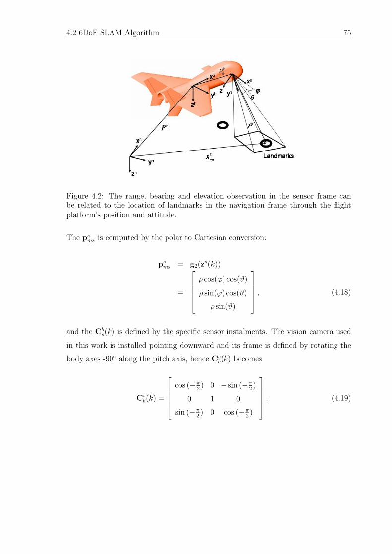
4.2 6DoF SLAM Algorithm 75
Figure 4.2: The range, bearing and elevation observation in the sensor frame canbe related to the location of landmarks in the navigation frame through the flightplatform’s position and attitude.
The psms is computed by the polar to Cartesian conversion:
psms = g2(zs(k))
=
⎡⎢⎢⎢⎣ρ cos(ϕ) cos(ϑ)
ρ sin(ϕ) cos(ϑ)
ρ sin(ϑ)
⎤⎥⎥⎥⎦ , (4.18)
and the Cbs(k) is defined by the specific sensor instalments. The vision camera used
in this work is installed pointing downward and its frame is defined by rotating the
body axes -90◦ along the pitch axis, hence Csb(k) becomes
Csb(k) =
⎡⎢⎢⎢⎣
cos (−π2) 0 − sin (−π
2)
0 1 0
sin (−π2) 0 cos (−π
2)
⎤⎥⎥⎥⎦ . (4.19)
4.2 6DoF SLAM Algorithm 76
Then Cbs(k) is the transpose of this matrix:
Cbs(k) = CsT
b (k) =
⎡⎢⎢⎢⎣
0 0 −1
0 1 0
1 0 0
⎤⎥⎥⎥⎦ . (4.20)
4.2.4 Nonlinear Observation Model
The on-board range, bearing and elevation sensor provides relative observations be-
tween vehicle and landmarks. The nonlinear observation model relates these obser-
vations to the state as
z(k) = h(x(k),v(k)), (4.21)
where h(·, ·) is the non-linear observation model at time k, and v(k) is the observation
noise vector.
As the observation model predicts the range, bearing, and elevation for the ith
landmark, it becomes only a function of the ith landmark state and vehicle state.
Additionally, the sensor noise in range, bearing and elevation can be assumed additive.
Thus Equation 4.21 is further simplified as
zi(k) = h(xv(k),xmi(k)) + vi(k), (4.22)
where zi(k) and vi(k) are the ith observation and its associated noise in range, bearing
and elevation with zero mean and variance of R(k).
The predicted range, bearing, and elevation between the vehicle and ith landmark
4.2 6DoF SLAM Algorithm 77
can be obtained by taking an inverse of Equations 4.17 and 4.18:
zi(k) =[
zρ(k) zϕ(k) zϑ(k)]T
= g−12 (g−1
1 (xv,xmi))
= (g−12 ◦ g−1
1 )(xv,xmi), (4.23)
where the inverse functions are obtained as
g−12 (k) =
⎡⎢⎢⎢⎣
√x2 + y2 + z2
tan−1(y/x)
tan−1(z/√x2 + y2)
⎤⎥⎥⎥⎦ , (4.24)
with psms = [ x y z ]T obtained from the inverse function of g1(k) as,
g−11 (k) = Cs
b(k)Cbn(k)
[xnmi(k) − pn(k) − Cn
b (k)pbsb
]. (4.25)
The Jacobian of ∇hx(k) with respect to the current vehicle and map state can be
derived from the nonlinear observation Equation 4.21 by applying a chain rule to the
composite inverse function,
∇hx(k) =
⎡⎢⎢⎢⎣
∂ρ(k)∂pn(k)
∂ρ(k)∂vn(k)
∂ρ(k)∂ψn(k)
∂ϕ(k)∂pn(k)
∂ϕ(k)∂vn(k)
∂ϕ(k)∂ψn(k)
∂ϑ(k)∂pn(k)
∂ϑ(k)∂vn(k)
∂ϑ(k)∂ψn(k)
⎤⎥⎥⎥⎦ (4.26)
= ∇xg−12 (g−1
1 (x(k))) (4.27)
= [∇yg−12 (y(k))][∇xg
−11 (x(k))] (4.28)
where y(k) = g−11 ((x(k))) is defined in Equation 4.25 and g−1
2 (k) is defined in Equa-
4.2 6DoF SLAM Algorithm 78
tion 4.24. The Jacobians of these functions are computed as,
∇g−12 (k) =
⎡⎢⎢⎢⎢⎣
x√x2+y2+z2
y√x2+y2+z2
z√x2+y2+z2
−yx2+y2
xx2+y2
0
−xz(x2+y2+z2)
√x2+y2
−yz(x2+y2+z2)
√x2+y2
√x2+y2
x2+y2+z2
⎤⎥⎥⎥⎥⎦ (4.29)
∇g−11 (k) =
[−(Cn
bCbs)T 0
∂CsbC
bn(xmi−p)
∂ψn(k−1)· · · (Cn
bCbs)T · · ·
]. (4.30)
The sub-matrix in the third column is also a Jacobian of the relative position in the
sensor frame with respect to the Euler angle and can also be computed using a similar
method as in Equation 4.13,
∂{Csb(k)C
bn(k)(x
nmi(k) − pnv (k))}
∂ψn(k)=
⎡⎢⎢⎢⎣
∂xs(k)∂φ(k)
∂xs(k)∂θ(k)
∂xs(k)∂ψ(k)
∂ys(k)∂φ(k)
∂ys(k)∂θ(k)
∂ys(k)∂ψ(k)
∂zs(k)∂φ(k)
∂zs(k)∂θ(k)
∂zs(k)∂ψ(k)
⎤⎥⎥⎥⎦ (4.31)
where [ xs ys zs ]T = CsbC
bn(xmi − p) is used. Then the elements of this Jacobian
are
∂xs
∂φ= xn(CφSψ − SφSθCψ) + yn(−CφCψ − SφSθSψ) − zn(SφCθ)
∂xs
∂θ= xn(CφCθCψ) + yn(CφCθSψ) − zn(CφSθ)
∂xs
∂ψ= xn(SφCψ − CφSθSψ) + yn(SφSψ + CφSθCψ)
∂ys
∂φ= xn(SφSψ + CφSθCψ) + yn(−SφCψ + CφSθSψ) + znCφCθ;
∂ys
∂θ= xn(SφCθCψ) + yn(SφCθSψ) − zn(SφSθ)
∂ys
∂ψ= xn(−CφCψ − SφSθSψ) + yn(−CφSψ + SφSθCψ)

4.2 6DoF SLAM Algorithm 79
∂zs
∂φ= 0
∂zs
∂θ= xn(SθCψ) + yn(SθSψ) + zn(Cθ)
∂zs
∂ψ= xn(CθSψ) − yn(CθCψ),
where [ xn yn zn ]T = xmi(k) − p(k) is used for simplicity.
4.2.5 Prediction
Now the state estimate and its covariance matrix from time k − 1 to time k can be
propagated using the nonlinear process model and its associated Jacobian matrices:
x(k | k − 1) = f(x(k − 1 | k − 1),u(k),0) (4.32)
P(k | k − 1) = ∇fx(k)P(k − 1|k − 1)∇fx(k)T + ∇fw(k)Q(k)∇fw(k)T . (4.33)
4.2.6 Estimation
When an observation occurs, and if it is successfully associated with one of the land-
marks registered within the filter, then the observation is used to update the state
vector and its covariance matrix,
x(k | k) = x(k | k − 1) + W(k)ν(k) (4.34)
P(k | k) = [I − W(k)∇hx(k)]P(k | k − 1)[I − W(k)∇hx(k)]T
+W(k)R(k)WT (k). (4.35)
4.2 6DoF SLAM Algorithm 80
where the innovation vector, ν(k), Kalman gain, W(k), and innovation covariance,
S(k) are computed by
ν(k) = z(k) − h(x(k | k − 1),0) (4.36)
W(k) = P(k | k − 1)∇hxT (k)S−1(k) (4.37)
S(k) = ∇hx(k)P(k | k − 1)∇hxT (k) + R(k). (4.38)
4.2.7 Data Association
Data association is a process that finds out the correspondence between observations
at time k and landmarks registered within the filter state. Correct correspondence of
the sensed landmark observations to mapped landmarks is essential for consistent map
construction, and a single false match will invalidate the entire estimation process.
Association validation is performed in observation space. As a statistical valida-
tion gate, the Normalised Innovation Square (NIS) (also known as the Mahalanobis
distance) is used to associate observations [8]. The NIS (γ) is computed by
γ = ν(k)TS−1(k)ν(k). (4.39)
Given an innovation and its covariance with the assumption of Gaussian distribution,
γ forms a χ2 (chi-square) distribution. If γ is less than a predefined threshold, then the
observation and the landmark that were used to form the innovation are associated.
The threshold value is obtained from the standard χ2 tables and is chosen based on
the confidence level required. Thus for example, a 99.5% confidence level, and for
a state vector which includes three states of range, bearing, and elevation, then the
threshold is 12.8. The associated innovation is now used to update the state and
covariance.
4.2 6DoF SLAM Algorithm 81
4.2.8 New Landmark Augmentation
If an observation is not matched to any registered landmarks, then it is a new land-
mark observation. It is then dynamically augmented into both the state vector and
the covariance matrix through an initialisation function g1(k) defined in Equation
4.17. The augmented state can be represented as
xaug(k) = G(xv(k),xm(k), z(k)) (4.40)
=
⎡⎢⎢⎢⎣
xv(k)
xm(k)
g1(xv(k), z(k))
⎤⎥⎥⎥⎦ (4.41)
where the initialised landmark position is only dependent on the vehicle state and
observation which results in sparse matrix in g1(k).
The initialised landmark state becomes highly correlated to the vehicle state. That
is the vehicle uncertainty in position and attitude directly affects the uncertainty
in initialised landmark position. Due to this fact, the cross-correlation should be
calculated properly in the augmented covariance matrix.
The augmented covariance matrix can now be obtained using the covariance trans-
formation method using the Jacobian of the initialisation function, such as,
Paug(k) = ∇G
⎡⎢⎢⎢⎣
Pvv(k) Pvm(k) 0
Pmv(k) Pmm(k) 0
0 0 R(k)
⎤⎥⎥⎥⎦∇GT (4.42)
where ∇G is computed from Equation 4.40 by
∇G =
⎡⎢⎢⎢⎣
Iv 0 0
0 Im 0
∇vg1(k) 0 ∇zg1(k)
⎤⎥⎥⎥⎦ (4.43)
4.2 6DoF SLAM Algorithm 82
Hence Equation 4.42 becomes
Paug(k) =
⎡⎢⎢⎢⎣
Pvv(k) Pvm(k) (∇vg1(k)Pvv(k))T
Pmv(k) Pmm(k) (∇vg1(k)Pvm(k))T
∇vg1(k)Pvv(k) ∇vg1(k)Pvm(k) Υ(k)
⎤⎥⎥⎥⎦ (4.44)
where
Υ(k) = ∇vg1(k)Pvv(k)∇vg1(k)T + ∇zg1(k)R(k)∇zg1(k)
T (4.45)
and ∇vg1(k) and ∇zg1(k) are Jacobians for the landmark initialisation function with
respect to the vehicle state and observation, respectively:
∇vg1(k) =[
I 0∂{Cn
b (k)(pbsb+Cb
s(k)psms(k))}
∂ψ(k)
](4.46)
∇zg1(k) = (CnbC
bs)(∇zg2(k)) (4.47)
and the Jacobian of the initialisation function with respect to the Euler angle has the
same form as in Equation 4.13 by replacing the fn(k) with xb(k) = pbsb + Cbsp
sms.
From Equation 4.44, the correlation between the vehicle and the landmark can
be clearly observed. This correlation structure is maintained and evolved during the
SLAM operation. When the vehicle closes the navigation loop with a detection of a
former landmark, the accumulated INS drifts during this loop become observable and
can be estimated, which in turn reduces the uncertainties in landmarks via this cor-
relation. By doing this, the initial uncertainty in the landmark due to the INS errors
can be effectively removed and it monotonically decreases toward the lower bound
which is determined by the initial vehicle uncertainty upon the first observation.
Using these equations the 6DoF EKF SLAM can fulfill its cycle of prediction and
estimation.
4.2 6DoF SLAM Algorithm 83
4.2.9 Error Analysis on the Initialised Landmarks
The initialised new landmark position contains errors due to various error sources
such as the platform’s position and attitude error, sensor measurement error, sensor
misalignment error and sensor lever-arm error. As the initialised landmark positions
are again used to estimate the platform’s state in the SLAM filter, it will be instructive
to analyse the individual error contribution to the landmark position in Equation 4.17
[72].
The error in the landmark position is defined as the difference between the pre-
dicted position pnm and true position pnm:
δpnm � pnm − pnm (4.48)
Perturbing Equation 4.17 with the errors and subtracting it from the true landmark
position gives
δpnm = (pn − pn) + (Cnb p
bsb − Cn
bpbsb) + (Cn
b Cbsp
sms − Cn
bCbsp
sms) (4.49)
Using the predicted DCM as the true DCM misaligned by errors:
Cnb � (I − [δψn×])Cn
b (4.50)
Cbs � (I − [δθbs×])Cb
s (4.51)
where [δψn×] and [δθbs×] are the INS attitude error and sensor misalignment error
expressed in skew-symmetric form, respectively. Using these, Equation 4.49 can now
be rewritten as
δpnm = δpn + Cnb δp
bsb +
Cnb [p
bsb×]δψn + Cn
bCbsδp
sms + Cn
bCbs[p
sms×](δψn + δθbs). (4.52)
4.2 6DoF SLAM Algorithm 84
Equation 4.52 relates each error contribution to the targeting accuracy of the
landmark where
• δpn is the position error of the INS in the navigation frame.
• Cnb δp
bsb is the position error in the navigation frame due to uncertainty in the
lever-arm vector between sensor instalments position and the vehicle centre.
This error can be reduced by precisely measuring the lever-arm vector.
• Cnb [p
bsb×]δψn is the position error in the navigation frame due to the INS atti-
tude error, scaled by the sensor lever-arm vector.
• CnbC
bsδp
sms is the error in the relative position between the vehicle and the
landmark in the navigation frame, which is computed from the range, bearing
and elevation measurement.
• CnbC
bs[p
sms×](δψn + δθbs) is the landmark positioning error due to the INS at-
titude error and the sensor misalignment, scaled by the measured relative dis-
tance.
From this analysis, it can be observed that the position error of the vehicle is
directly reflected to the initialised landmark position error, which establishes the cor-
relation structure between the vehicle and the landmark. It can also be seen that
the dominant error source is the last term where the attitude error and sensor mis-
alignment are scaled by the relative distance between the vehicle and the landmark.
That is, the further the landmark is located from the vehicle, the larger the landmark
position error introduced. Hence to minimise this error, accurate gyros are required
within the IMU, however, this in turn increases the cost of the sensor. Alternatively,
if there are constant observations of landmarks occurring, the growth of the attitude
error of the platform can be constrained effectively.
4.3 Indirect 6DoF SLAM Algorithm 85
4.3 Indirect 6DoF SLAM Algorithm
This section provides an alternative solution to SLAM’s computational complexity,
not from the perspective of map management techniques, but by focusing on the
filter’s structure and model, and recasting the SLAM algorithm into an indirect filter
implementation [42]. In doing so the navigation structure provided is exceedingly
computationally efficient even for highly non-linear, highly dynamic systems.
The problem is solved by separating the SLAM filter from the main navigation
loop and, instead of estimating the states of the vehicle and landmarks, the filter
estimates the errors in these states. This is accomplished by perturbing the dynamic
equations which govern the platform and map models, hence linearising an otherwise
highly non-linear system. Figure 4.3 compares the flow diagrams for both the direct
and indirect filter structures. Although the heart of the SLAM algorithm is exactly
the same, the major differences include the ability to constantly have navigation
information since this is provided outside of the filter structure. The benefits of the
indirect SLAM can be summarised:
• The system becomes more suitable for real-time processing. The main INS
loop can provide continuous navigation data within fixed time intervals. The
SLAM update cycle whose computation time increases according to the map
size won’t disrupt the main INS loop and time propagation algorithms can be
used to match information at appropriate times.
• The SLAM prediction cycle exploits the low-dynamic characteristics of the INS
errors. As a result the sample rate for the SLAM prediction cycle is much lower
than that of the direct filter. The better the accuracy of the IMU, the less
frequently the prediction cycle needs to run. It is for this reason that most
of the research conducted on INS applications has focused on error analysis
techniques [24]. Furthermore, if the only modelled error in both the INS and
the map is Gaussian white noise (no deterministic errors such as bias) then only
the covariance matrix needs to be propagated through the prediction cycle.
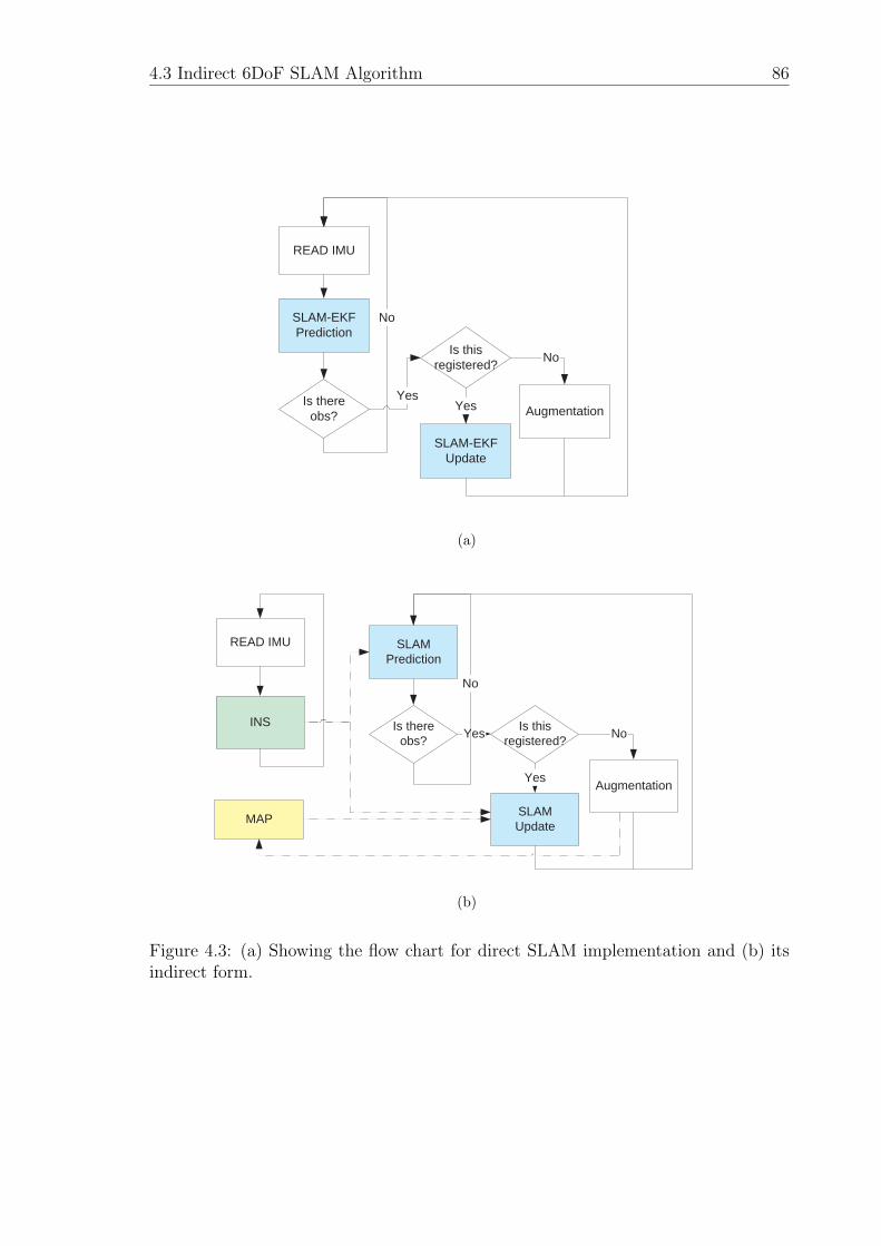
4.3 Indirect 6DoF SLAM Algorithm 86
READ IMU
SLAM-EKFPrediction
Is thereobs? Augmentation
Is thisregistered?
SLAM-EKFUpdate
Yes
No
Yes
No
(a)
READ IMU
INS Is thereobs?
Augmentation
Is thisregistered?
SLAMUpdate
Yes
NoYes
No
SLAMPrediction
MAP
(b)
Figure 4.3: (a) Showing the flow chart for direct SLAM implementation and (b) itsindirect form.
4.3 Indirect 6DoF SLAM Algorithm 87
• The system is more robust to faults. When faults occur within the SLAM filter,
due to mismatch in observations, the INS loop can still provide a continuous
navigation solution to other tasks. The faults may be isolated, and the SLAM
filter can be re-initialised which would in turn increase system integrity.
• The system takes on a greater level of modularity. The INS error model has
been well developed and is fairly independent of specific INS algorithms [24].
As a result, the SLAM filter can be easily augmented to existing navigation
systems, and in fact other aiding filters can be attached easily.
4.3.1 External Inertial Navigation Loop
In the indirect SLAM structure, the SLAM filter aids the external INS loop in a
complementary fashion. The inertial navigation algorithms developed in Chapter 3
are used to predict the high-dynamic vehicle states from the IMU measurements.
In this implementation a quaternion based strapdown INS algorithm is used:
⎡⎢⎢⎢⎣
pn(k)
vn(k)
q(k)
⎤⎥⎥⎥⎦ =
⎡⎢⎢⎢⎣
pn(k − 1) + vn(k − 1)�tvn(k − 1) + [q(k − 1) ⊗ f b(k) ⊗ q∗(k − 1) + gn]�t
q(k − 1) ⊗�q(k)
⎤⎥⎥⎥⎦ ,(4.53)
where the first-order integration is used with �t being the time for the position and
velocity update interval, q∗(k − 1) is a quaternion conjugate for the vector trans-
formation, and �q(k) is a delta quaternion during the attitude update interval as
defined in Equation 3.28.
4.3.2 External Map
In the indirect SLAM structure, the map is maintained outside the SLAM filter and
is treated as an external map database. The SLAM filter estimates the errors in the
4.3 Indirect 6DoF SLAM Algorithm 88
map and feeds back the correction term. If a new landmark is observed, the external
map is dynamically augmented with the new landmark position, and the SLAM filter
covariance is also augmented with an initial uncertainty and correlation.
4.3.3 Augmented Error State
In indirect SLAM, the state vector in Equation 4.1 is now defined as the error state:
δx(k) = [ δxv(k) δxm(k) ]T . (4.54)
The error state of the vehicle, δxv(k), comprises the errors in the INS indicated
position, velocity and attitude expressed in the navigation frame:
δxv(k) = [ δpn(k) δvn(k) δψn(k) ]T . (4.55)
The error state of the map, δxm(k), also comprises the errors in 3D landmark
positions in the navigation frame. The size of state is also dynamically augmented
with the new landmark error after the initialisation process,
δxm(k) = [ δxnTm1(k) δxnTm2(k) . . . δxnTmN(k) ]T , (4.56)
where N is the current number of registered landmarks in the filter and each state
consists of a 3D position error [ δxn δyn δzn ]T .
4.3.4 Error Process Model
The linearised SLAM system in discrete time can be written as
δx(k) = F(k)δx(k − 1) + G(k)w(k) (4.57)
4.3 Indirect 6DoF SLAM Algorithm 89
where δx is the error state vector, F(k) is the system transition matrix, G(k) is the
system noise input matrix and w(k) is the system noise vector which represents the
instrument noise with any unmodelled errors with noise strength Q(k).
This equation can be obtained by discretising the continuous SLAM error model.
Since the landmarks are assumed stationary, their errors can be modelled as a random
constant:
δxnm = 0m. (4.58)
Using this landmark error model and the INS error models from Equations 3.59,
3.66, and 3.67, the SLAM error equation can now be constructed in continuous time:
⎡⎢⎢⎢⎢⎢⎣
δpn
δvn
δψn
δxnm
⎤⎥⎥⎥⎥⎥⎦ =
⎡⎢⎢⎢⎢⎢⎣
δvn
−2ωnin × δvn + Cnb fb × δψn + Cn
b δfb
−Cnb δω
bib
0m
⎤⎥⎥⎥⎥⎥⎦ . (4.59)
The discrete state transition function, F(tk), can be computed by applying an
integration factor method and a first-order integration during time �t (note the low
dynamic characteristics of the INS error which makes this approximation a valid one):
F(tk) = exp
(∫ tk
tk−1
f(t)dt
)≈ exp (f(tk−1)�t), (4.60)
where f(t) is the state transition function in continuous time which is defined from
Equation 4.59. Expanding the exponential function and approximating to the second-
order term gives
F(tk) ≈ I + f(tk−1)�t+(f(tk−1)�t)2
2!. (4.61)
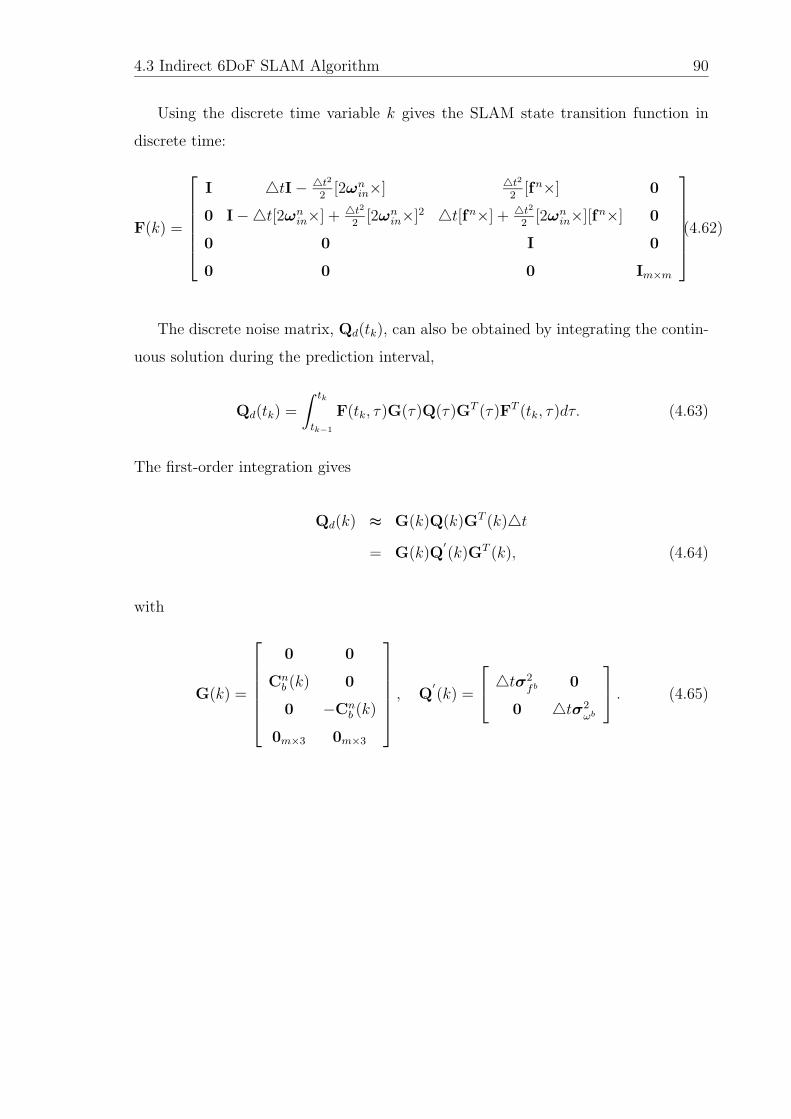
4.3 Indirect 6DoF SLAM Algorithm 90
Using the discrete time variable k gives the SLAM state transition function in
discrete time:
F(k) =
⎡⎢⎢⎢⎢⎢⎣
I �tI − �t22
[2ωnin×] �t22
[fn×] 0
0 I −�t[2ωnin×] + �t22
[2ωnin×]2 �t[fn×] + �t22
[2ωnin×][fn×] 0
0 0 I 0
0 0 0 Im×m
⎤⎥⎥⎥⎥⎥⎦ .(4.62)
The discrete noise matrix, Qd(tk), can also be obtained by integrating the contin-
uous solution during the prediction interval,
Qd(tk) =
∫ tk
tk−1
F(tk, τ)G(τ)Q(τ)GT (τ)FT (tk, τ)dτ. (4.63)
The first-order integration gives
Qd(k) ≈ G(k)Q(k)GT (k)�t= G(k)Q
′(k)GT (k), (4.64)
with
G(k) =
⎡⎢⎢⎢⎢⎢⎣
0 0
Cnb (k) 0
0 −Cnb (k)
0m×3 0m×3
⎤⎥⎥⎥⎥⎥⎦ , Q
′(k) =
⎡⎣ �tσ2
fb 0
0 �tσ2ωb
⎤⎦ . (4.65)
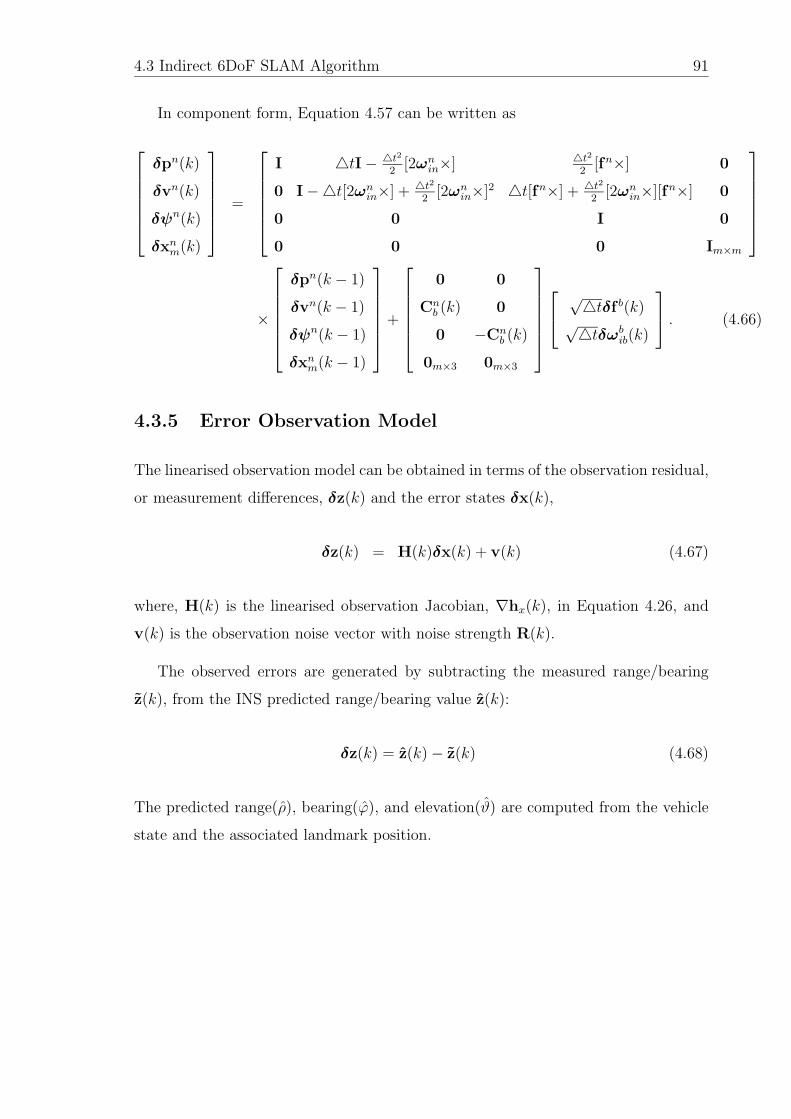
4.3 Indirect 6DoF SLAM Algorithm 91
In component form, Equation 4.57 can be written as
⎡⎢⎢⎢⎢⎢⎣
δpn(k)
δvn(k)
δψn(k)
δxnm(k)
⎤⎥⎥⎥⎥⎥⎦ =
⎡⎢⎢⎢⎢⎢⎣
I �tI − �t22
[2ωnin×] �t22
[fn×] 0
0 I −�t[2ωnin×] + �t22
[2ωnin×]2 �t[fn×] + �t22
[2ωnin×][fn×] 0
0 0 I 0
0 0 0 Im×m
⎤⎥⎥⎥⎥⎥⎦
×
⎡⎢⎢⎢⎢⎢⎣
δpn(k − 1)
δvn(k − 1)
δψn(k − 1)
δxnm(k − 1)
⎤⎥⎥⎥⎥⎥⎦+
⎡⎢⎢⎢⎢⎢⎣
0 0
Cnb (k) 0
0 −Cnb (k)
0m×3 0m×3
⎤⎥⎥⎥⎥⎥⎦⎡⎣ √�tδf b(k)
√�tδωbib(k)
⎤⎦ . (4.66)
4.3.5 Error Observation Model
The linearised observation model can be obtained in terms of the observation residual,
or measurement differences, δz(k) and the error states δx(k),
δz(k) = H(k)δx(k) + v(k) (4.67)
where, H(k) is the linearised observation Jacobian, ∇hx(k), in Equation 4.26, and
v(k) is the observation noise vector with noise strength R(k).
The observed errors are generated by subtracting the measured range/bearing
z(k), from the INS predicted range/bearing value z(k):
δz(k) = z(k) − z(k) (4.68)
The predicted range(ρ), bearing(ϕ), and elevation(ϑ) are computed from the vehicle
state and the associated landmark position.
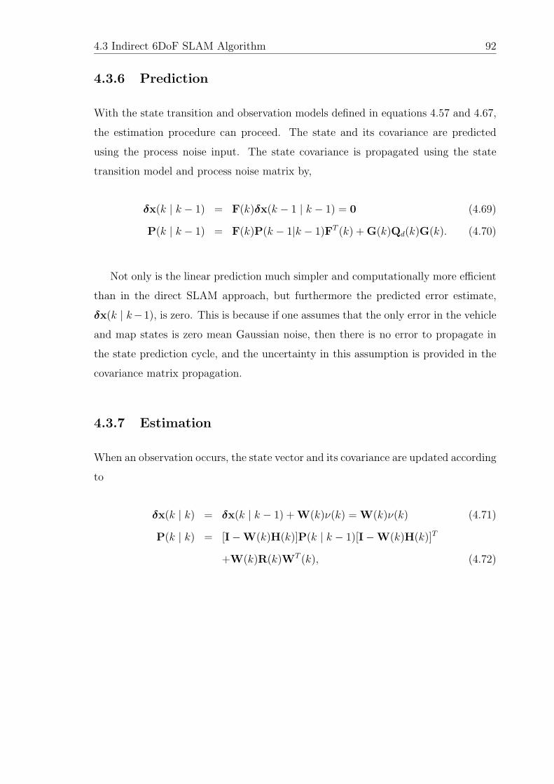
4.3 Indirect 6DoF SLAM Algorithm 92
4.3.6 Prediction
With the state transition and observation models defined in equations 4.57 and 4.67,
the estimation procedure can proceed. The state and its covariance are predicted
using the process noise input. The state covariance is propagated using the state
transition model and process noise matrix by,
δx(k | k − 1) = F(k)δx(k − 1 | k − 1) = 0 (4.69)
P(k | k − 1) = F(k)P(k − 1|k − 1)FT (k) + G(k)Qd(k)G(k). (4.70)
Not only is the linear prediction much simpler and computationally more efficient
than in the direct SLAM approach, but furthermore the predicted error estimate,
δx(k | k−1), is zero. This is because if one assumes that the only error in the vehicle
and map states is zero mean Gaussian noise, then there is no error to propagate in
the state prediction cycle, and the uncertainty in this assumption is provided in the
covariance matrix propagation.
4.3.7 Estimation
When an observation occurs, the state vector and its covariance are updated according
to
δx(k | k) = δx(k | k − 1) + W(k)ν(k) = W(k)ν(k) (4.71)
P(k | k) = [I − W(k)H(k)]P(k | k − 1)[I − W(k)H(k)]T
+W(k)R(k)WT (k), (4.72)
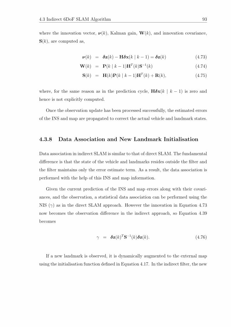
4.3 Indirect 6DoF SLAM Algorithm 93
where the innovation vector, ν(k), Kalman gain, W(k), and innovation covariance,
S(k), are computed as,
ν(k) = δz(k) − Hδx(k | k − 1) = δz(k) (4.73)
W(k) = P(k | k − 1)HT (k)S−1(k) (4.74)
S(k) = H(k)P(k | k − 1)HT (k) + R(k), (4.75)
where, for the same reason as in the prediction cycle, Hδx(k | k − 1) is zero and
hence is not explicitly computed.
Once the observation update has been processed successfully, the estimated errors
of the INS and map are propagated to correct the actual vehicle and landmark states.
4.3.8 Data Association and New Landmark Initialisation
Data association in indirect SLAM is similar to that of direct SLAM. The fundamental
difference is that the state of the vehicle and landmarks resides outside the filter and
the filter maintains only the error estimate term. As a result, the data association is
performed with the help of this INS and map information.
Given the current prediction of the INS and map errors along with their covari-
ances, and the observation, a statistical data association can be performed using the
NIS (γ) as in the direct SLAM approach. However the innovation in Equation 4.73
now becomes the observation difference in the indirect approach, so Equation 4.39
becomes
γ = δz(k)TS−1(k)δz(k). (4.76)
If a new landmark is observed, it is dynamically augmented to the external map
using the initialisation function defined in Equation 4.17. In the indirect filter, the new
4.3 Indirect 6DoF SLAM Algorithm 94
landmark error state is initialised with a zero vector and the covariance is initialised
using Equation 4.42 as in the direct SLAM approach.
4.3.9 Feedback Error Correction
Once the observation estimation has been processed successfully, the estimated errors
are now fed to the external INS loop and the map for correction.
From the definitions of the error in position and velocity of the INS as in Equation
3.60, the corrected position, pnc (k), and corrected velocity, vnc (k), are obtained by
subtracting the errors:
pnc (k) = pn(k) − δpn(k) (4.77)
vnc (k) = vn(k) − δvn(k). (4.78)
The attitude correction is performed from the estimated misalignment angle. Since
the quaternion is used as the attitude parameter in the external INS loop, an equiva-
lent error quaternion, δq(k), should be constructed from the estimated misalignment
angles, that is,
δq(k) =
⎡⎢⎢⎢⎢⎢⎣
cos( δψx
2) cos( δψy
2) cos( δψz
2) + sin( δψx
2) sin( δψy
2) sin( δψz
2)
sin( δψx
2) cos( δψy
2) cos( δψz
2) − cos( δψx
2) sin( δψy
2) sin( δψz
2)
cos( δψx
2) sin( δψy
2) cos( δψz
2) + sin( δψx
2) cos( δψy
2) sin( δψz
2)
cos( δψx
2) cos( δψy
2) sin( δψz
2) + sin( δψx
2) sin( δψy
2) cos( δψz
2)
⎤⎥⎥⎥⎥⎥⎦ , (4.79)
with the misalignment angles, δψn(k) = [δψx δψy δψz ]T . Applying the small angle
approximation for the trigonometric functions and ignoring the product terms of two
4.4 DDF 6DoF SLAM 95
small angles, gives
δq(k) ≈
⎡⎢⎢⎢⎢⎢⎣
1
δψx
2
δψy
2
δψz
2
⎤⎥⎥⎥⎥⎥⎦ . (4.80)
Therefore the corrected quaternion, qc(k), is obtained by multiplying the error
quaternion to the current quaternion:
qc(k) = δq(k) ⊗ q(k). (4.81)
The corrected map positions are directly obtained by subtracting the estimated
map position errors from the current positions:
(xnm)c(k) = xnm(k) − δxnm(k). (4.82)
Using these equations the indirect 6DoF SLAM filter can fulfill its cycle of pre-
diction and estimation with the external INS loop and the map.
4.4 DDF 6DoF SLAM
Previous works on DDF SLAM were only for a 3DoF platform using a tricycle model
[59]. In this thesis, DDF SLAM is expanded to the full 6DoF model with the same
information filter framework described in Section 2.6 [39] and the details of the DDF
architecture can be found in [59].
In this architecture the information is propagated to all vehicles or nodes in the
network via point-to-point links with no loops in the network, as illustrated in Figure
4.4 DDF 6DoF SLAM 96
4.4(a). The internal structure of each of these sensing nodes is illustrated in Figure
4.4(b) where each node contains a local filter node, a channel manager and a channel
filter. The details of these modules are provided in [59, 73].
In DDF 6DoF SLAM, two important facts can be exploited [59]:
• The platform to platform cross information is zero provided the vehicles do not
sense each other.
• The global map information is the sum of the map information on each platform
in the system.
It should be noted that although the assumption was made that the platforms do not
sense each other, they are correlated in state space as they are navigating using a
common map. In information space however, the cross information between platforms
becomes zero. This is due to the fact that having information about one platform
does not provide any information about any other platforms if platforms do not use
relative observations of each other for localisation.
In addition, as the global map information is simply the sum of the contributions
from each platform (which is the result from the additive property in the information
filter update), the map information is all that needs to be communicated between
platforms. As the cross information between multiple platforms is zero, it is not
necessary for a platform to augment the vehicle states of any other node. Platforms
merely receive map information from others in the network and fuse this with their
own local map. The DDF SLAM problem can be depicted as shown in Figure 4.5
where multiple aircraft are all communicating map information and localising them-
selves within the common map.
In the hybrid-space SLAM architecture as discussed in [59], the local SLAM node
operates in state space, but the inter-platform updates is performed in information
space. Hence the 6DoF SLAM algorithm developed in Section 4.2 can be directly
applied to the local SLAM node. Firstly, the estimated map and its covariance from
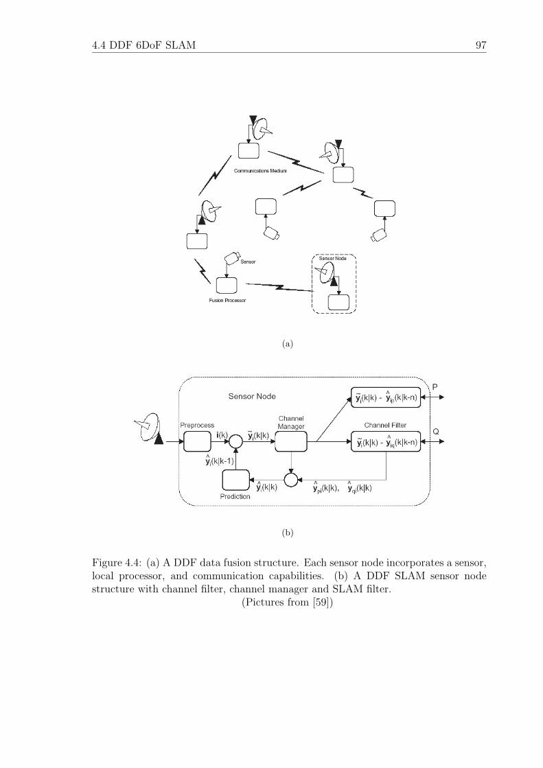
4.4 DDF 6DoF SLAM 97
(a)
(b)
Figure 4.4: (a) A DDF data fusion structure. Each sensor node incorporates a sensor,local processor, and communication capabilities. (b) A DDF SLAM sensor nodestructure with channel filter, channel manager and SLAM filter.
(Pictures from [59])
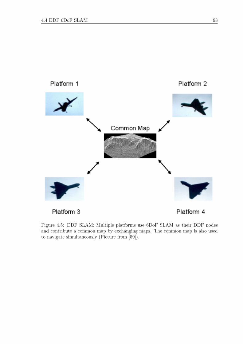
4.4 DDF 6DoF SLAM 98
Figure 4.5: DDF SLAM: Multiple platforms use 6DoF SLAM as their DDF nodesand contribute a common map by exchanging maps. The common map is also usedto navigate simultaneously (Picture from [59]).
4.4 DDF 6DoF SLAM 99
the local SLAM node are converted into its information equivalent for propagation.
That is, given the map estimate, xm(k | k), and covariance matrix, Pmm(k | k),defined in Equation 4.4 in local 6DoF SLAM, the information matrix and estimate
of the map are constructed as
Ymm(k | k) = P−1mm(k | k) (4.83)
ym(k | k) = P−1mm(k | k)xm(k | k). (4.84)
It is the map information quantities Ymm(k | k) and ym(k | k) that are communicated
between nodes (It should be noted that they are not simply the map component of
the information estimate and matrix due to the matrix inversion of P(k | k) [59]).
A channel filter is then used to keep a record of the map information that nodes
have in common. When information arrives to the channel filter, it determines the
information gain to send by subtracting the existing channel estimate from the newly
arrived data. This new information, written as Imm(k | k) and im(k | k) is the output
from the channel filter which is propagated to the network [59].
In other nodes in the DDF network, this transmitted map information is firstly
processed within the channel filter to form the new information and is then used to
update its local filter in information space:
Y(k | k) =
⎡⎣ Yvv(k | k) Yvm(k | k)
Ymv(k | k) Ymm(k | k)
⎤⎦+
⎡⎣ 0vv 0vm
0mv Imm(k | k)
⎤⎦ (4.85)
y(k | k) =
⎡⎣ yv(k | k)
ym(k | k)
⎤⎦+
⎡⎣ 0v
im(k | k)
⎤⎦ . (4.86)
The local SLAM estimate in information space is then converted back to state
space:
P(k | k) = Y−1(k | k)x(k | k) = P(k | k)y(k | k). (4.87)
4.5 Summary 100
The local SLAM node continues its cycle using the local inertial data and local
observations in state space, however with a common global map. If the vehicles build
maps in completely separate areas, the common map is simply the addition of each
adjoint map. However, if the vehicles share some part of the map, the accuracy of
the global map will be improved, and the vehicle accuracy as well because of the cor-
relation structure between the vehicle and map. This DDF map building approach
however, has a limitation in that the vehicles should start navigation from initial
locations expressed in common coordinates. If each vehicle starts its navigation at a
completely unknown location, then the map information cannot be exchanged with
other maps because the landmarks are represented in two different coordinate sys-
tems, hence they cannot be associated to other maps. This problem can be overcame
by matching the geometry of features between maps, or by at least knowing the ini-
tial pose of the UAVs with respect to some origin (as it is conducted in this thesis,
where the vehicle initial locations are known but the mission is in a GPS denied en-
vironment). It however requires a way to choose or negotiate the common coordinate
system in implementing a fully decentralised and modular SLAM network.
4.5 Summary
This chapter has developed the underlying algorithm structures for airborne SLAM
that will be used in subsequent chapters.
The SLAM algorithm was developed using the INS equations in the earth-fixed
frame (represented here as the navigation frame) and Euler or quaternion angle atti-
tude representation. The nonlinear sensor observation model was also provided from
the vehicle state and landmark position. The Jacobian matrices were explicitly de-
rived from the nonlinear vehicle model and range/bearing observation model. The
data association and new feature augmentation method were provided. The accuracy
of the initialised landmark position was also analysed from the nonlinear relationship
between the vehicle and landmark. The indirect 6DoF SLAM algorithm, which is
4.5 Summary 101
defined not on the total state but on the error state of the vehicle and map, was also
developed. This SLAM structure becomes quite suitable for real-time SLAM imple-
mentation due to the filter structure being decoupled from the main INS loop. Finally,
the DDF SLAM algorithm for airborne applications was provided by using the 6DoF
SLAM algorithm for the local node and exchanging map information between other
nodes on other platforms.
Chapter 5
GNSS/Inertial AirborneNavigation
5.1 Introduction
The Global Navigation Satellite System (GNSS) is a spaceborne, radio navigation
system. Its world-wide coverage, availability, and high accuracy makes it one of
history’s most revolutionary developments. In airborne navigation, its complementary
characteristics to the inertial navigation system make it an excellent aiding source.
Although the theory of GNSS aided inertial navigation is not new, its success-
ful implementation to autonomous airborne systems using low-cost sensors is still a
challenging area, and it requires theoretical and practical considerations regarding
sensor quality, fusion algorithm and structure, and an understanding of the dynamic
environments. This chapter will provide details of the GNSS/Inertial algorithm along
with the theoretical and practical solutions to the related problems.
Firstly, a fusion structure for a GNSS/Inertial system will be presented. The
indirect filter structure is presented by using the linearised error dynamic model of
the INS and the navigation outputs from the GNSS system.
Secondly, the spatial/temporal observation matching processes between the GNSS
measured and INS predicted observation are provided. The spatial offset arises from
5.2 GNSS Overview 103
the lever-arm of the GNSS antenna, and the temporal offset results from the latency
in the GNSS solution. Their error contributions is analysed for the real system.
Finally, the altitude vulnerability of the GNSS is described from real-flight results.
To overcome this, a baro-altimeter is augmented to the GNSS/Inertial system by
formulating the baro-altimeter error model.
5.2 GNSS Overview
GNSS utilises the concept of time-of-arrival (TOA) measurements from the satellites
to the user’s antenna to determine the user’s position, velocity and time [36]. That
is, by precisely measuring the time it takes for a signal transmitted by satellites at a
known location to reach a user receiver, then multiplied by the speed of the light, the
range information can be obtained. From multiple range measurements, the user’s
position can be computed [36].
Two GNSS are currently operational: The Global Positioning System (GPS) and
the Global Navigation Satellite System (GLONASS) developed respectively by the
United States and the Russian Federation. In addition, the European Union (EU)
has a plan to launch its first experimental satellite for the GALILEO system, the
European GNSS, in 2005 and to achieve full operational capability by 2008 [21].
More detailed information can be found in [3, 54, 61]. As GLONASS is functionally
similar to GPS with slightly different technical specifications, only a brief overview
about GPS is presented.
GPS is managed by the United States Air Force, providing significant benefits to
civilian applications. The Standard Positioning Service (SPS), which utilises a coarse
acquisition (C/A) code on the 1575.42Mhz (L1) frequency, is designed to provide
accurate positioning capability for civilian users throughout the world. A Precise
Position Service (PPS), which utilises the Precise Code (P-code) on the 1227.60Mhz
(L2) frequency which has not been authorised for public use, is designed to provide
5.3 GNSS/Inertial Integration 104
more accurate positioning capability to users authorised by the Unites States Depart-
ment of Defense (DoD). The 24 satellites operate in near circular orbits at 20, 200km
with an inclination angle of 55◦ to the equator and each satellite completes an orbit
in 12hr sidereal time. Each satellite broadcasts a pseudo-random code with a data
message that the user receiver processes to obtain satellite position and status. The
ephemeris data of each satellite is broadcasted as part of the data message and the
user can calculate the satellite location precisely. By precisely matching the pseudo-
random code generated in the receiver and satellite, the TOA can be computed. With
the information of the satellite position and the TOA measurements from at least four
satellites, the user position and time bias can be computed.
A GPS modernisation plan was announced in January 1999 to extend the capabil-
ity. The main components in this plan consist of adding two new navigation signals
that will be available for civilian use: another C/A code at 1227.60Mhz (L2) and a
new signal at 1176.45Mhz (L5). The L5 signal will provide significant benefits for
civilian aviation with the existing L1 C/A signal via its increased availability, iono-
spheric correction and interference mitigation. All three civil signals will be available
for initial operational capability by 2010, and for full operational capability by around
2013.
5.3 GNSS/Inertial Integration
There have been extensive theoretical and practical research activities focussing on
the fusion of GNSS and INS to improve the accuracy and reduce the cost of navigation
systems [40, 62, 69, 74]. The synergistic effects in the GNSS/Inertial integrated system
are well reported in many studies [25, 78]. The current trends are incorporating a lower
cost, or equivalently lower quality, inertial sensor with a higher performance GNSS
sensor with deeply-coupled integration structures [62].
The low-cost, light, and compact-sized GNSS/Inertial system is an ideal naviga-
tion system for the UAV platform which has only a limited payload capacity and also
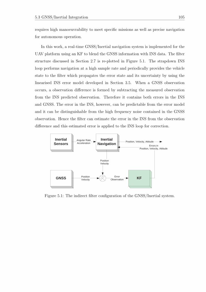
5.3 GNSS/Inertial Integration 105
requires high manoeuvrability to meet specific missions as well as precise navigation
for autonomous operation.
In this work, a real-time GNSS/Inertial navigation system is implemented for the
UAV platform using an KF to blend the GNSS information with INS data. The filter
structure discussed in Section 2.7 is re-plotted in Figure 5.1. The strapdown INS
loop performs navigation at a high sample rate and periodically provides the vehicle
state to the filter which propagates the error state and its uncertainty by using the
linearised INS error model developed in Section 3.5. When a GNSS observation
occurs, a observation difference is formed by subtracting the measured observation
from the INS predicted observation. Therefore it contains both errors in the INS
and GNSS. The error in the INS, however, can be predictable from the error model
and it can be distinguishable from the high frequency noise contained in the GNSS
observation. Hence the filter can estimate the error in the INS from the observation
difference and this estimated error is applied to the INS loop for correction.
InertialSensors
InertialNavigation
GNSS KF
Angular RateAcceleration
PositionVelocity
Errors inPosition, Velocity, Attitude
PositionVelocity
ErrorObservation
Position, Velocity, Attitude
Figure 5.1: The indirect filter configuration of the GNSS/Inertial system.
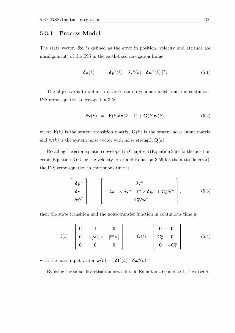
5.3 GNSS/Inertial Integration 106
5.3.1 Process Model
The state vector, δx, is defined as the error in position, velocity and attitude (or
misalignment) of the INS in the earth-fixed navigation frame:
δx(k) = [ δpn(k) δvn(k) δψn(k) ]T . (5.1)
The objective is to obtain a discrete state dynamic model from the continuous
INS error equations developed in 3.5:
δx(k) = F(k)δx(k − 1) + G(k)w(k), (5.2)
where F(k) is the system transition matrix, G(k) is the system noise input matrix
and w(k) is the system noise vector with noise strength Q(k).
Recalling the error equation developed in Chapter 3 (Equation 3.67 for the position
error, Equation 3.66 for the velocity error and Equation 3.59 for the attitude error),
the INS error equation in continuous time is
⎡⎢⎢⎢⎣δpn
δvn
δψn
⎤⎥⎥⎥⎦ =
⎡⎢⎢⎢⎣
δvn
−2ωnin × δvn + fn × δψn + Cnb δf
b
−Cnb δω
b
⎤⎥⎥⎥⎦ , (5.3)
then the state transition and the noise transfer function in continuous time is
f(t) =
⎡⎢⎢⎢⎣
0 I 0
0 −2[ωnin×] [fn×]
0 0 0
⎤⎥⎥⎥⎦ , G(t) =
⎡⎢⎢⎢⎣
0 0
Cnb 0
0 −Cnb
⎤⎥⎥⎥⎦ (5.4)
with the noise input vector w(k) = [ δf b(k) δωb(k) ]T .
By using the same discretisation procedure in Equation 4.60 and 4.61, the discrete
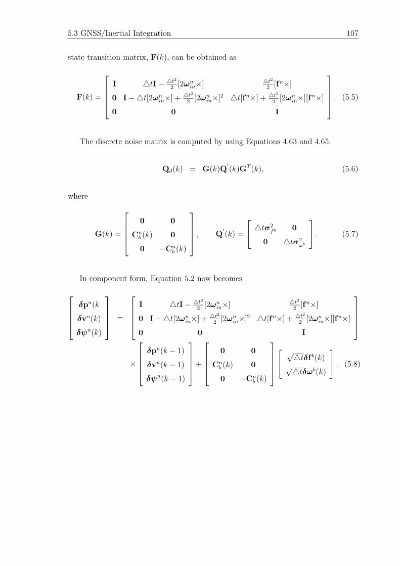
5.3 GNSS/Inertial Integration 107
state transition matrix, F(k), can be obtained as
F(k) =
⎡⎢⎢⎢⎣
I �tI − �t22
[2ωnin×] �t22
[fn×]
0 I −�t[2ωnin×] + �t22
[2ωnin×]2 �t[fn×] + �t22
[2ωnin×][fn×]
0 0 I
⎤⎥⎥⎥⎦ . (5.5)
The discrete noise matrix is computed by using Equations 4.63 and 4.65:
Qd(k) = G(k)Q′(k)GT (k), (5.6)
where
G(k) =
⎡⎢⎢⎢⎣
0 0
Cnb (k) 0
0 −Cnb (k)
⎤⎥⎥⎥⎦ , Q
′(k) =
⎡⎣ �tσ2
fb 0
0 �tσ2ωb
⎤⎦ . (5.7)
In component form, Equation 5.2 now becomes
⎡⎢⎢⎢⎣δpn(k
δvn(k)
δψn(k)
⎤⎥⎥⎥⎦ =
⎡⎢⎢⎢⎣
I �tI − �t22
[2ωnin×] �t22
[fn×]
0 I −�t[2ωnin×] + �t22
[2ωnin×]2 �t[fn×] + �t22
[2ωnin×][fn×]
0 0 I
⎤⎥⎥⎥⎦
×
⎡⎢⎢⎢⎣δpn(k − 1)
δvn(k − 1)
δψn(k − 1)
⎤⎥⎥⎥⎦+
⎡⎢⎢⎢⎣
0 0
Cnb (k) 0
0 −Cnb (k)
⎤⎥⎥⎥⎦⎡⎣ √�tδf b(k)
√�tδωb(k)
⎤⎦ . (5.8)
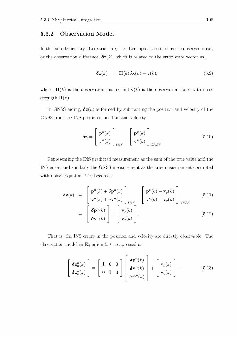
5.3 GNSS/Inertial Integration 108
5.3.2 Observation Model
In the complementary filter structure, the filter input is defined as the observed error,
or the observation difference, δz(k), which is related to the error state vector as,
δz(k) = H(k)δx(k) + v(k), (5.9)
where, H(k) is the observation matrix and v(k) is the observation noise with noise
strength R(k).
In GNSS aiding, δz(k) is formed by subtracting the position and velocity of the
GNSS from the INS predicted position and velocity:
δz =
⎡⎣ pn(k)
vn(k)
⎤⎦INS
−⎡⎣ pn(k)
vn(k)
⎤⎦GNSS
. (5.10)
Representing the INS predicted measurement as the sum of the true value and the
INS error, and similarly the GNSS measurement as the true measurement corrupted
with noise, Equation 5.10 becomes,
δz(k) =
⎡⎣ pn(k) + δpn(k)
vn(k) + δvn(k)
⎤⎦INS
−⎡⎣ pn(k) − vp(k)
vn(k) − vv(k)
⎤⎦GNSS
(5.11)
=
⎡⎣ δpn(k)δvn(k)
⎤⎦+
⎡⎣ vp(k)
vv(k)
⎤⎦ . (5.12)
That is, the INS errors in the position and velocity are directly observable. The
observation model in Equation 5.9 is expressed as
⎡⎣ δznp (k)δznv (k)
⎤⎦ =
⎡⎣ I 0 0
0 I 0
⎤⎦⎡⎢⎢⎢⎣δpn(k)
δvn(k)
δψn(k)
⎤⎥⎥⎥⎦+
⎡⎣ vp(k)
vv(k)
⎤⎦ . (5.13)
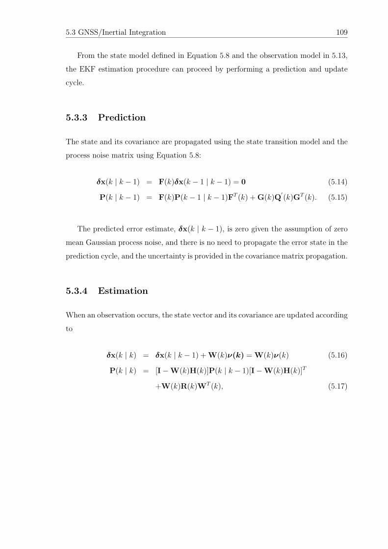
5.3 GNSS/Inertial Integration 109
From the state model defined in Equation 5.8 and the observation model in 5.13,
the EKF estimation procedure can proceed by performing a prediction and update
cycle.
5.3.3 Prediction
The state and its covariance are propagated using the state transition model and the
process noise matrix using Equation 5.8:
δx(k | k − 1) = F(k)δx(k − 1 | k − 1) = 0 (5.14)
P(k | k − 1) = F(k)P(k − 1 | k − 1)FT (k) + G(k)Q′(k)GT (k). (5.15)
The predicted error estimate, δx(k | k − 1), is zero given the assumption of zero
mean Gaussian process noise, and there is no need to propagate the error state in the
prediction cycle, and the uncertainty is provided in the covariance matrix propagation.
5.3.4 Estimation
When an observation occurs, the state vector and its covariance are updated according
to
δx(k | k) = δx(k | k − 1) + W(k)ν(k) = W(k)ν(k) (5.16)
P(k | k) = [I − W(k)H(k)]P(k | k − 1)[I − W(k)H(k)]T
+W(k)R(k)WT (k), (5.17)
5.3 GNSS/Inertial Integration 110
where the innovation vector, ν(k), the Kalman weight, W(k), and the innovation
covariance, S(k), are computed as,
ν(k) = δz(k) − Hδx(k | k − 1) = δz(k) (5.18)
W(k) = P(k | k − 1)HT (k)S−1(k) (5.19)
S(k) = H(k)P(k | k − 1)HT (k) + R(k). (5.20)
For the same reason as in the prediction cycle, H(k)δx(k | k− 1) is zero and hence is
not computed, the estimated error becomes simply a weighted measurement residual.
5.3.5 Feedback Error Correction
Once the observation update has been processed successfully, the estimated errors of
the INS are propagated to correct the external INS loop.
Similar to indirect SLAM, the corrected position and velocity are
pnc (k) = pn(k) − δpn(k) (5.21)
vnc (k) = vn(k) − δvn(k). (5.22)
For attitude correction, if a quaternion approach is used, the corrected quaternion,
qc(k), is
qc(k) = δq(k) ⊗ q(k), (5.23)
where the error quaternion
δq(k) ≈
[1 δψx
2
δψy
2δψz
2
]T(5.24)
and the misalignment angles are δψn(k) = [ δψx δψy δψz ]T .
5.4 Observation Matching 111
If the DCM approach is used, the attitude correction can be directly applied from
the definition of the misalignment angle
(Cnb )c(k) = (I − [δψ(k)×])−1Cn
b (k) (5.25)
= (I + [δψ(k)×])Cnb (k), (5.26)
where [δψ(k)×] is a skew symmetric matrix.
5.4 Observation Matching
The observation matching process is required in Equation 5.10, where the INS indi-
cated observation is subtracted from the GNSS observation to generate the observa-
tion difference. As with any statistical estimation algorithm, a biased observation will
cause significant errors in the filter performance. Two issues in observation match-
ing are considered: 1) observation latency and 2) the lever-arm offset. Their error
contributions to the real system implemented in this thesis are analysed.
5.4.1 Observation Latency
Latency in the GNSS solution is inevitable due to the internal signal processing
and computational time. Data transmission over the serial link also introduces an
additional latency in the GNSS output. The delay varies depending on receiver types
but typical values are 50ms for internal computation and 30ms for serial output
processing, resulting in 80ms delay. In airborne applications, such as the Brumby
Mk-III which flies at a speed of 50m/s, an 80ms delay can cause a 4m position error
between the GNSS and INS. More importantly, the velocity vector can change its
direction rapidly during maneuvers, which can result in a significant mismatch in the
velocity observation. As the INS attitude error is highly correlated to the velocity
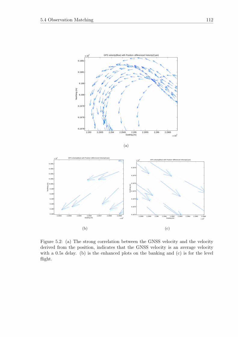
5.4 Observation Matching 112
2.293 2.2935 2.294 2.2945 2.295 2.2955 2.296 2.2965
x 105
6.1678
6.1678
6.1679
6.168
6.168
6.1681
6.1681
x 106
Easting (m)
Nor
thin
g (m
)
GPS velocity(Blue) with Position−differenced Velocity(Cyan)
(a)
2.2933 2.2934 2.2935 2.2936 2.2937 2.2938 2.2939
x 105
6.168
6.168
6.168
6.168
6.168
6.168
6.1681
6.1681
6.1681
6.1681
6.1681
x 106
Easting (m)
Nor
thin
g (m
)
GPS velocity(Blue) with Position−differenced Velocity(Cyan)
(b)
2.2958 2.2959 2.296 2.2961 2.2962 2.2963 2.2964 2.2965 2.2966
x 105
6.1675
6.1675
6.1675
6.1675
6.1676
6.1676
6.1676
x 106
Easting (m)
Nor
thin
g (m
)
GPS velocity(Blue) with Position−differenced Velocity(Cyan)
(c)
Figure 5.2: (a) The strong correlation between the GNSS velocity and the velocityderived from the position, indicates that the GNSS velocity is an average velocitywith a 0.5s delay. (b) is the enhanced plots on the banking and (c) is for the levelflight.
5.4 Observation Matching 113
error, this incorrectly observed velocity error can result in a incorrectly estimated
attitude error.
To overcome this latency, most GNSS receivers provide a 1 Pulse Per Second
(1PPS) hardware signal which is precisely aligned to the GNSS time. Only the
interrupt latency in the navigation computer contributes to the delay in processing
this signal. The real-time kernel used in this work has an interrupt latency under
a microsecond. An interrupt handler wakes up on this hardware signal and fetches
the INS solution which corresponds to the GNSS observation. To get more precise
synchronisation at the 1PPS event, an interpolation algorithm can be used from the
last updated INS solution and the elapsed time till the 1PPS event. By this method,
the GNSS observation is precisely synchronised to the INS data within a half sampling
time of the IMU, that is 1.2ms.
In addition to the latency mentioned above, a different type of latency can also
occur in the GNSS velocity. If the velocity is computed from the position solution,
instead of from the Doppler shift measurement, the data can be delayed approxi-
mately half a second compared to the position. Figure 5.2 shows the velocity latency
observed in the real system. The measured velocity shows a strong correlation with
the computed velocity derived from the position difference. Thus it is obvious that
the velocity from the GNSS receiver used in this work is averaged velocity, while the
velocity of the INS is an instantaneous quantity. Hence there will always be the pos-
sibility of observation matching errors especially under maneuvering. In the actual
GNSS/Inertial implementation described in Chapter 6, the GNSS velocity observa-
tion is matched with a half-second old INS velocity from the 1PPS event. However, its
contribution to the filter update is devalued by increasing the velocity measurement
noise in Rv(k).
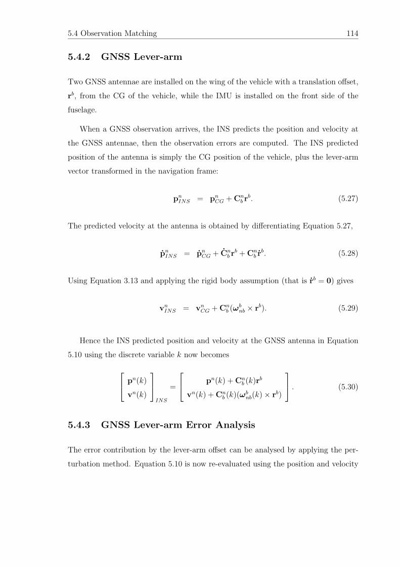
5.4 Observation Matching 114
5.4.2 GNSS Lever-arm
Two GNSS antennae are installed on the wing of the vehicle with a translation offset,
rb, from the CG of the vehicle, while the IMU is installed on the front side of the
fuselage.
When a GNSS observation arrives, the INS predicts the position and velocity at
the GNSS antennae, then the observation errors are computed. The INS predicted
position of the antenna is simply the CG position of the vehicle, plus the lever-arm
vector transformed in the navigation frame:
pnINS = pnCG + Cnb r
b. (5.27)
The predicted velocity at the antenna is obtained by differentiating Equation 5.27,
pnINS = pnCG + Cnb r
b + Cnb r
b. (5.28)
Using Equation 3.13 and applying the rigid body assumption (that is rb = 0) gives
vnINS = vnCG + Cnb (ω
bnb × rb). (5.29)
Hence the INS predicted position and velocity at the GNSS antenna in Equation
5.10 using the discrete variable k now becomes
⎡⎣ pn(k)
vn(k)
⎤⎦INS
=
⎡⎣ pn(k) + Cn
b (k)rb
vn(k) + Cnb (k)(ω
bnb(k) × rb)
⎤⎦ . (5.30)
5.4.3 GNSS Lever-arm Error Analysis
The error contribution by the lever-arm offset can be analysed by applying the per-
turbation method. Equation 5.10 is now re-evaluated using the position and velocity
5.4 Observation Matching 115
observation compensated for by the lever-arm.
Firstly, the position observation is computed by substituting Equation 5.27 into
Equation 5.10 for the INS predicted quantities, and by using the perturbation method:
δznp = (pn + Cnb r
b)INS − pnGNSS (5.31)
= {(pn + δpn) + (I − [δψn×])Cnb (r
b + δrb)}INS−{pn − vp}GNSS. (5.32)
After manipulation and ignoring the product of two small error terms, gives
δznp = δpn + Cnb [r
b×]δψn + Cnb δr
b + vp. (5.33)
Equation 5.33 relates each error contribution to the position error in the filter input:
• δpn is the position error in the INS.
• Cnb [r
b×]δψn is the position error from the INS attitude error scaled by the
GNSS lever-arm vector.
• Cbnδr
nb is the position error from the error in the lever-arm vector.
• vp is the position error in the GNSS position which is assumed to be an unbiased
high frequency noise.
The first term is what the filter tries to estimate from the error dynamic model and
the second term relates the attitude error to the filter observation via the lever-arm
vector. The third term can be minimised by measuring the lever-arm vector precisely.
The velocity observation to the filter can also be obtained by using a similar
5.4 Observation Matching 116
method. Perturbing Equation 5.29 gives,
δznv = {vn + Cnb (ω
bnb × rb)}INS − vnGNSS (5.34)
= {(vn + δvn) + (I − [δψn×])Cnb (ω
bnb + δωbnb) × (rb + δrb)}INS
−{vn − vv}GNSS. (5.35)
Ignoring the product of two small error terms gives
δznv = δvn + Cnb [ω
bnb×][rb×]δψn + Cn
b [ωbnb×]δrb − Cn
b [rb×]δωbnb + vv. (5.36)
Equation 5.36 relates each error contribution to the velocity difference to the filter
input:
• δvn is the velocity error in the INS.
• Cnb [ω
bnb×][rb×]δψn is the velocity error from the INS attitude error scaled by
the lever-arm vector and the rotation rate of the vehicle.
• Cnb [ω
bnb×]δrb is the velocity error from the error in the lever-arm vector.
• Cnb [r
b×]δωbnb is the velocity error from the angular rate’s error, which is equal
to the gyro error in the earth fixed frame.
• vv is the error in the GNSS velocity which is assumed to be an unbiased high
frequency noise.
Hence the more precise observation model for Equation 5.10 can be obtained by
using Equations 5.33 and 5.36,
δz =
⎡⎣ δpn + Cn
b [rb×]δψn + Cn
b δrb
δvn + Cnb [ω
bnb×][rb×]δψn + Cn
b [ωbnb×]δrb − Cn
b [rb×]δωbnb
⎤⎦+
⎡⎣ vp
vv
⎤⎦(5.37)
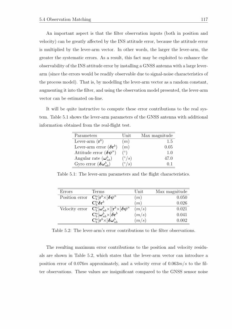
5.4 Observation Matching 117
An important aspect is that the filter observation inputs (both in position and
velocity) can be greatly affected by the INS attitude error, because the attitude error
is multiplied by the lever-arm vector. In other words, the larger the lever-arm, the
greater the systematic errors. As a result, this fact may be exploited to enhance the
observability of the INS attitude error by installing a GNSS antenna with a large lever-
arm (since the errors would be readily observable due to signal-noise characteristics of
the process model). That is, by modelling the lever-arm vector as a random constant,
augmenting it into the filter, and using the observation model presented, the lever-arm
vector can be estimated on-line.
It will be quite instructive to compute these error contributions to the real sys-
tem. Table 5.1 shows the lever-arm parameters of the GNSS antenna with additional
information obtained from the real-flight test.
Parameters Unit Max magnitudeLever-arm (rb) (m) 1.5Lever-arm error (δrb) (m) 0.05Attitude error (δψn) (◦) 1.0Angular rate (ωbnb) (◦/s) 47.0Gyro error (δωbnb) (◦/s) 0.1
Table 5.1: The lever-arm parameters and the flight characteristics.
Errors Terms Unit Max magnitudePosition error Cn
b [rb×]δψn (m) 0.050
Cnb δr
b (m) 0.026Velocity error Cn
b [ωbnb×][rb×]δψn (m/s) 0.021
Cnb [ω
bnb×]δrb (m/s) 0.041
Cnb [r
b×]δωbnb (m/s) 0.002
Table 5.2: The lever-arm’s error contributions to the filter observations.
The resulting maximum error contributions to the position and velocity residu-
als are shown in Table 5.2, which states that the lever-arm vector can introduce a
position error of 0.076m approximately, and a velocity error of 0.063m/s to the fil-
ter observations. These values are insignificant compared to the GNSS sensor noise
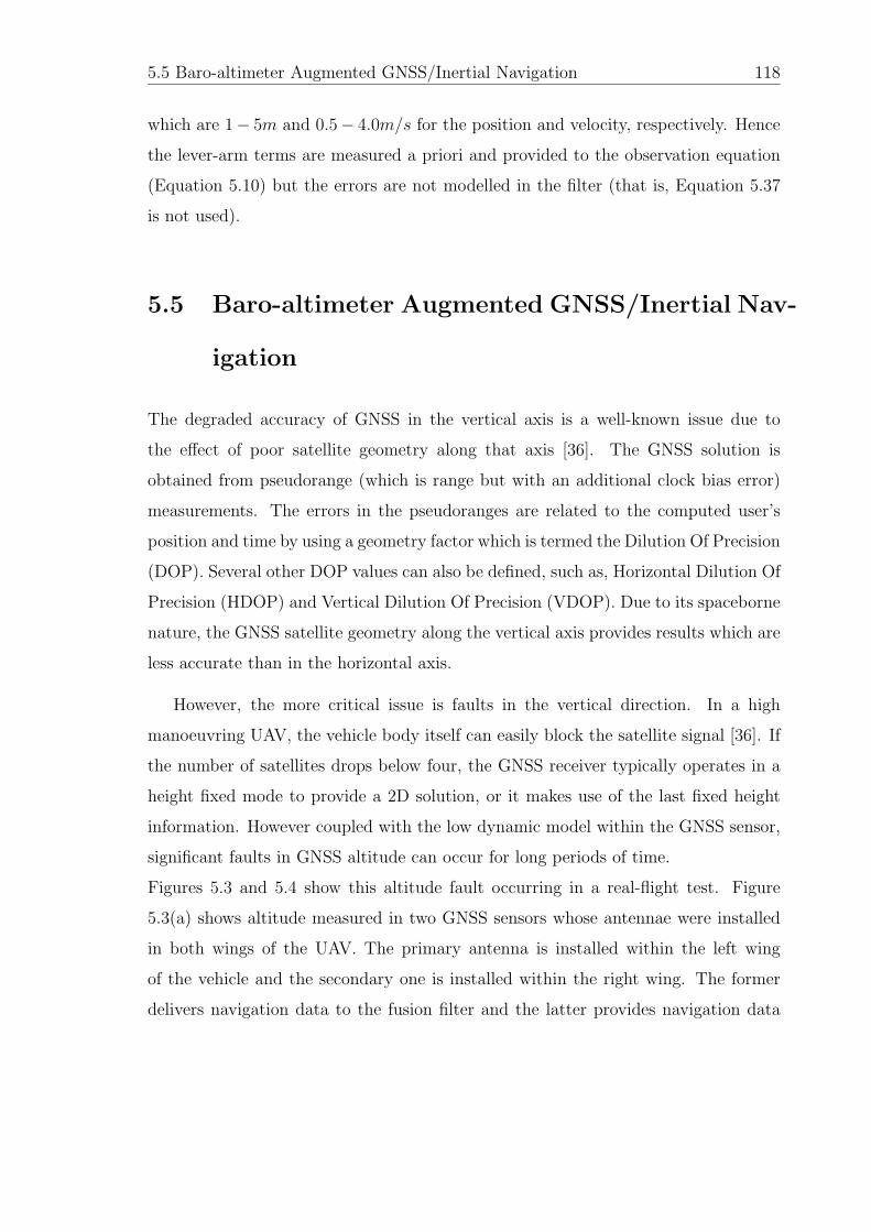
5.5 Baro-altimeter Augmented GNSS/Inertial Navigation 118
which are 1− 5m and 0.5− 4.0m/s for the position and velocity, respectively. Hence
the lever-arm terms are measured a priori and provided to the observation equation
(Equation 5.10) but the errors are not modelled in the filter (that is, Equation 5.37
is not used).
5.5 Baro-altimeter Augmented GNSS/Inertial Nav-
igation
The degraded accuracy of GNSS in the vertical axis is a well-known issue due to
the effect of poor satellite geometry along that axis [36]. The GNSS solution is
obtained from pseudorange (which is range but with an additional clock bias error)
measurements. The errors in the pseudoranges are related to the computed user’s
position and time by using a geometry factor which is termed the Dilution Of Precision
(DOP). Several other DOP values can also be defined, such as, Horizontal Dilution Of
Precision (HDOP) and Vertical Dilution Of Precision (VDOP). Due to its spaceborne
nature, the GNSS satellite geometry along the vertical axis provides results which are
less accurate than in the horizontal axis.
However, the more critical issue is faults in the vertical direction. In a high
manoeuvring UAV, the vehicle body itself can easily block the satellite signal [36]. If
the number of satellites drops below four, the GNSS receiver typically operates in a
height fixed mode to provide a 2D solution, or it makes use of the last fixed height
information. However coupled with the low dynamic model within the GNSS sensor,
significant faults in GNSS altitude can occur for long periods of time.
Figures 5.3 and 5.4 show this altitude fault occurring in a real-flight test. Figure
5.3(a) shows altitude measured in two GNSS sensors whose antennae were installed
in both wings of the UAV. The primary antenna is installed within the left wing
of the vehicle and the secondary one is installed within the right wing. The former
delivers navigation data to the fusion filter and the latter provides navigation data
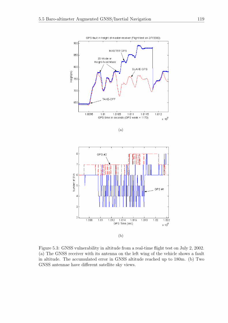
5.5 Baro-altimeter Augmented GNSS/Inertial Navigation 119
(a)
(b)
Figure 5.3: GNSS vulnerability in altitude from a real-time flight test on July 2, 2002.(a) The GNSS receiver with its antenna on the left wing of the vehicle shows a faultin altitude. The accumulated error in GNSS altitude reached up to 180m. (b) TwoGNSS antennae have different satellite sky views.
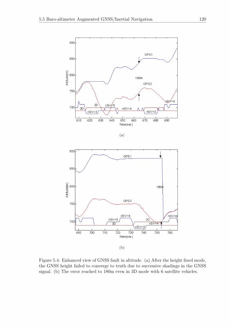
5.5 Baro-altimeter Augmented GNSS/Inertial Navigation 120
(a)
(b)
Figure 5.4: Enhanced view of GNSS fault in altitude. (a) After the height fixed mode,the GNSS height failed to converge to truth due to successive shadings in the GNSSsignal. (b) The error reached to 180m even in 3D mode with 6 satellite vehicles.
5.5 Baro-altimeter Augmented GNSS/Inertial Navigation 121
with additional raw measurement data. During flight, the vehicle undergoes successive
negative banking in the counter-clockwise direction. This imposes more signal shading
to the primary antenna and the number of satellites seen from it frequently drops
below four. In contrast, the secondary antenna has a better sky view than the primary
one and always sees more than six satellites as in Figure 5.3(b). During the first
several rounds, the primary receiver recovered the altitude accuracy within at most
ten seconds after the height fixed mode. After successive banking, however, the
height error failed to converge as in Figure 5.4(a). This is not a surprise because
low-cost GNSS sensors typically exploit a low-dynamic model and it takes time to
converge to the actual height from the fixed height mode. In land applications, the
height difference may be negligible if the undulation in terrain profile is not severe.
In airborne applications, however, there can be significant differences between the
GNSS indicated height and the actual height after the height-fixed mode. Around
181050sec (in GNSS second with week number 1173) in the plot, the error between
two GNSS outputs was around 100m after height-fixed operation. This error in the
primary receiver is accumulated during successive maneuvering and finally reached up
to 180m as shown in Figure 5.4(b). The nominal flight height is 110m above ground
and this kind of error is catastrophic for a low-altitude flying UAV.
There are several ways of tackling this fault: a statistical fault detection technique
as in [74], a redundant GNSS system (if for example a second GNSS receiver is placed
on the other wing to maximise the sky coverage, or below the wing), fusion of GNSS
raw measurement data (which does not require any low-dynamic assumption), or a
barometric altimeter augmentation.
In this thesis, a barometric altimeter (or baro-altimeter) is augmented to the
GNSS/Inertial system to enhance the altitude accuracy as shown in Figure 5.5. This
approach has several advantages:
• A baro-altimeter is a low-cost sensor (basically it is an air pressure sensor)
and is readily available for most airborne systems. It consists of an air pres-
sure/temperature sensor and a data acquisition system. From the measured air
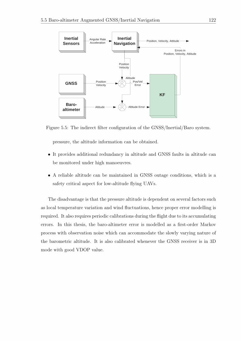
5.5 Baro-altimeter Augmented GNSS/Inertial Navigation 122
InertialSensors
InertialNavigation
GNSS
KF
Angular RateAcceleration
PositionVelocity
Errors inPosition, Velocity, Attitude
PositionVelocity
Pos/VelError
Position, Velocity, Attitude
Baro-altimeter
Altitude Altitude Error
Altitude
Figure 5.5: The indirect filter configuration of the GNSS/Inertial/Baro system.
pressure, the altitude information can be obtained.
• It provides additional redundancy in altitude and GNSS faults in altitude can
be monitored under high manoeuvres.
• A reliable altitude can be maintained in GNSS outage conditions, which is a
safety critical aspect for low-altitude flying UAVs.
The disadvantage is that the pressure altitude is dependent on several factors such
as local temperature variation and wind fluctuations, hence proper error modelling is
required. It also requires periodic calibrations during the flight due to its accumulating
errors. In this thesis, the baro-altimeter error is modelled as a first-order Markov
process with observation noise which can accommodate the slowly varying nature of
the barometric altitude. It is also calibrated whenever the GNSS receiver is in 3D
mode with good VDOP value.
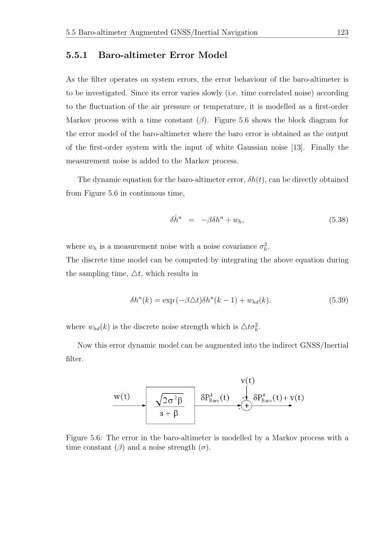
5.5 Baro-altimeter Augmented GNSS/Inertial Navigation 123
5.5.1 Baro-altimeter Error Model
As the filter operates on system errors, the error behaviour of the baro-altimeter is
to be investigated. Since its error varies slowly (i.e. time correlated noise) according
to the fluctuation of the air pressure or temperature, it is modelled as a first-order
Markov process with a time constant (β). Figure 5.6 shows the block diagram for
the error model of the baro-altimeter where the baro error is obtained as the output
of the first-order system with the input of white Gaussian noise [13]. Finally the
measurement noise is added to the Markov process.
The dynamic equation for the baro-altimeter error, δh(t), can be directly obtained
from Figure 5.6 in continuous time,
δhn = −βδhn + wh, (5.38)
where wh is a measurement noise with a noise covariance σ2h.
The discrete time model can be computed by integrating the above equation during
the sampling time, �t, which results in
δhn(k) = exp (−β�t)δhn(k − 1) + whd(k). (5.39)
where whd(k) is the discrete noise strength which is �tσ2h.
Now this error dynamic model can be augmented into the indirect GNSS/Inertial
filter.
Figure 5.6: The error in the baro-altimeter is modelled by a Markov process with atime constant (β) and a noise strength (σ).
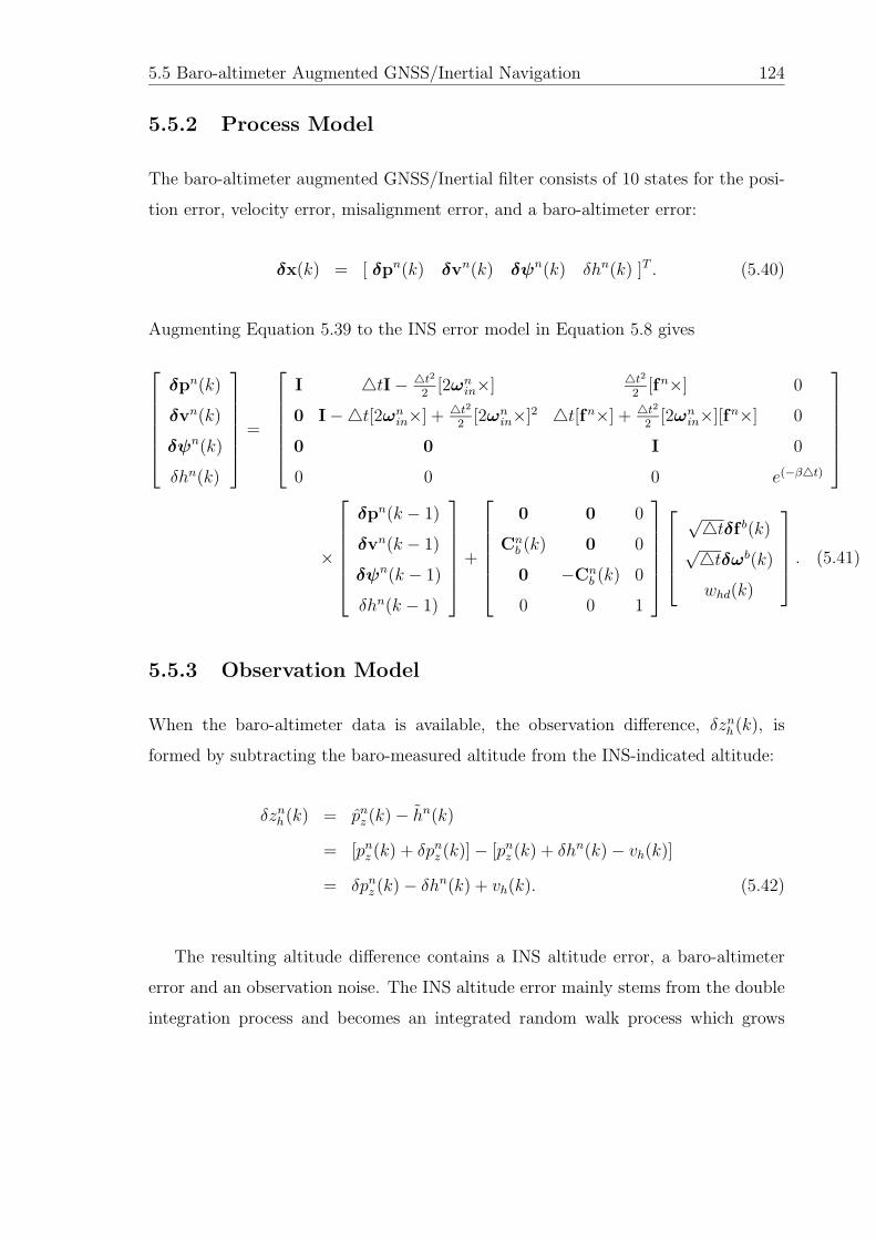
5.5 Baro-altimeter Augmented GNSS/Inertial Navigation 124
5.5.2 Process Model
The baro-altimeter augmented GNSS/Inertial filter consists of 10 states for the posi-
tion error, velocity error, misalignment error, and a baro-altimeter error:
δx(k) = [ δpn(k) δvn(k) δψn(k) δhn(k) ]T . (5.40)
Augmenting Equation 5.39 to the INS error model in Equation 5.8 gives
⎡⎢⎢⎢⎢⎢⎣
δpn(k)
δvn(k)
δψn(k)
δhn(k)
⎤⎥⎥⎥⎥⎥⎦ =
⎡⎢⎢⎢⎢⎢⎣
I �tI − �t22
[2ωnin×] �t22
[fn×] 0
0 I −�t[2ωnin×] + �t22
[2ωnin×]2 �t[fn×] + �t22
[2ωnin×][fn×] 0
0 0 I 0
0 0 0 e(−β�t)
⎤⎥⎥⎥⎥⎥⎦
×
⎡⎢⎢⎢⎢⎢⎣
δpn(k − 1)
δvn(k − 1)
δψn(k − 1)
δhn(k − 1)
⎤⎥⎥⎥⎥⎥⎦+
⎡⎢⎢⎢⎢⎢⎣
0 0 0
Cnb (k) 0 0
0 −Cnb (k) 0
0 0 1
⎤⎥⎥⎥⎥⎥⎦
⎡⎢⎢⎢⎣
√�tδf b(k)√�tδωb(k)whd(k)
⎤⎥⎥⎥⎦ . (5.41)
5.5.3 Observation Model
When the baro-altimeter data is available, the observation difference, δznh(k), is
formed by subtracting the baro-measured altitude from the INS-indicated altitude:
δznh(k) = pnz (k) − hn(k)
= [pnz (k) + δpnz (k)] − [pnz (k) + δhn(k) − vh(k)]
= δpnz (k) − δhn(k) + vh(k). (5.42)
The resulting altitude difference contains a INS altitude error, a baro-altimeter
error and an observation noise. The INS altitude error mainly stems from the double
integration process and becomes an integrated random walk process which grows
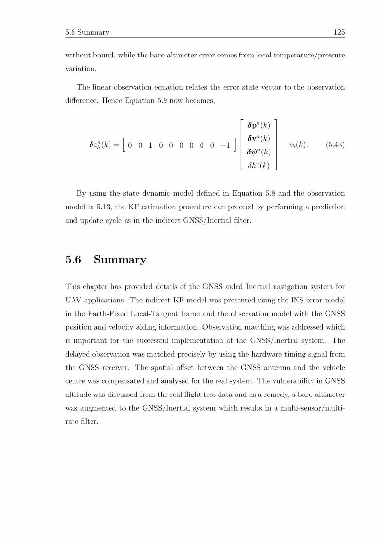
5.6 Summary 125
without bound, while the baro-altimeter error comes from local temperature/pressure
variation.
The linear observation equation relates the error state vector to the observation
difference. Hence Equation 5.9 now becomes,
δznh(k) =[
0 0 1 0 0 0 0 0 0 −1]⎡⎢⎢⎢⎢⎢⎣
δpn(k)
δvn(k)
δψn(k)
δhn(k)
⎤⎥⎥⎥⎥⎥⎦+ vh(k). (5.43)
By using the state dynamic model defined in Equation 5.8 and the observation
model in 5.13, the KF estimation procedure can proceed by performing a prediction
and update cycle as in the indirect GNSS/Inertial filter.
5.6 Summary
This chapter has provided details of the GNSS aided Inertial navigation system for
UAV applications. The indirect KF model was presented using the INS error model
in the Earth-Fixed Local-Tangent frame and the observation model with the GNSS
position and velocity aiding information. Observation matching was addressed which
is important for the successful implementation of the GNSS/Inertial system. The
delayed observation was matched precisely by using the hardware timing signal from
the GNSS receiver. The spatial offset between the GNSS antenna and the vehicle
centre was compensated and analysed for the real system. The vulnerability in GNSS
altitude was discussed from the real flight test data and as a remedy, a baro-altimeter
was augmented to the GNSS/Inertial system which results in a multi-sensor/multi-
rate filter.
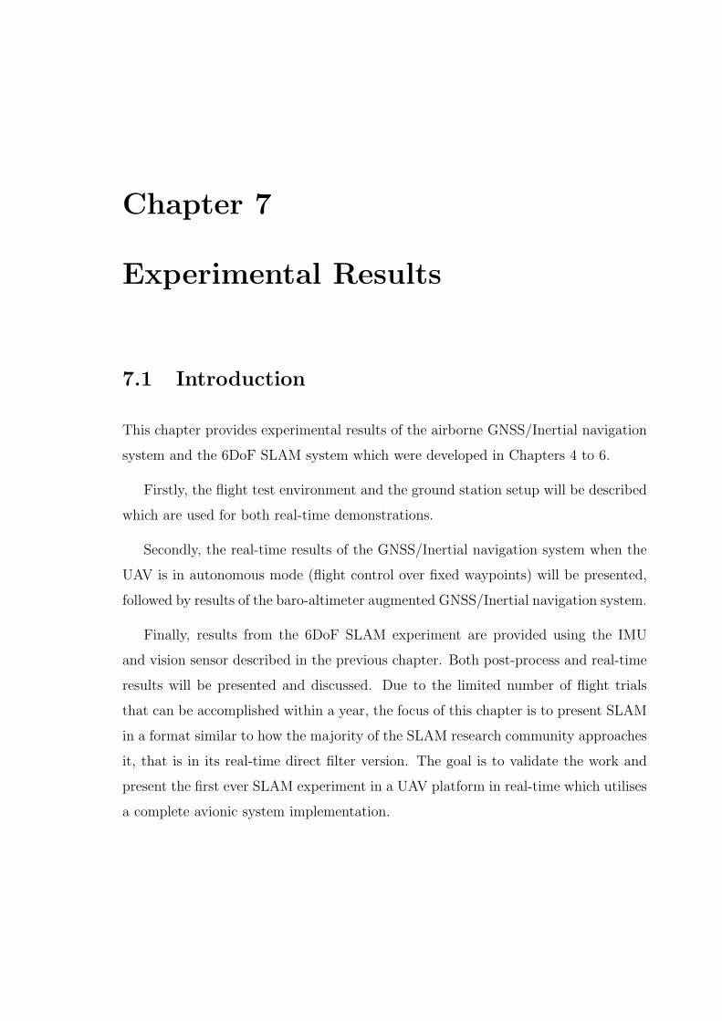
Chapter 7
Experimental Results
7.1 Introduction
This chapter provides experimental results of the airborne GNSS/Inertial navigation
system and the 6DoF SLAM system which were developed in Chapters 4 to 6.
Firstly, the flight test environment and the ground station setup will be described
which are used for both real-time demonstrations.
Secondly, the real-time results of the GNSS/Inertial navigation system when the
UAV is in autonomous mode (flight control over fixed waypoints) will be presented,
followed by results of the baro-altimeter augmented GNSS/Inertial navigation system.
Finally, results from the 6DoF SLAM experiment are provided using the IMU
and vision sensor described in the previous chapter. Both post-process and real-time
results will be presented and discussed. Due to the limited number of flight trials
that can be accomplished within a year, the focus of this chapter is to present SLAM
in a format similar to how the majority of the SLAM research community approaches
it, that is in its real-time direct filter version. The goal is to validate the work and
present the first ever SLAM experiment in a UAV platform in real-time which utilises
a complete avionic system implementation.
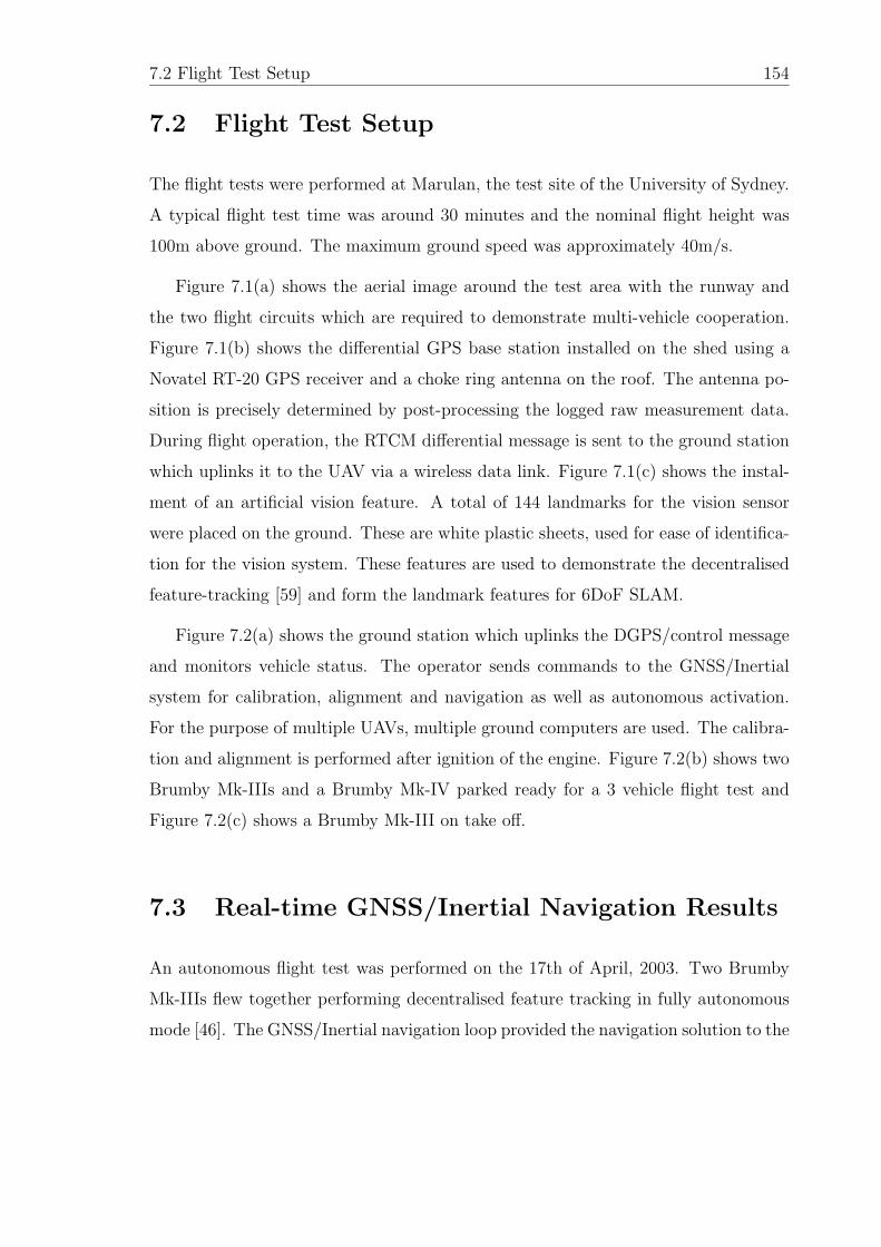
7.2 Flight Test Setup 154
7.2 Flight Test Setup
The flight tests were performed at Marulan, the test site of the University of Sydney.
A typical flight test time was around 30 minutes and the nominal flight height was
100m above ground. The maximum ground speed was approximately 40m/s.
Figure 7.1(a) shows the aerial image around the test area with the runway and
the two flight circuits which are required to demonstrate multi-vehicle cooperation.
Figure 7.1(b) shows the differential GPS base station installed on the shed using a
Novatel RT-20 GPS receiver and a choke ring antenna on the roof. The antenna po-
sition is precisely determined by post-processing the logged raw measurement data.
During flight operation, the RTCM differential message is sent to the ground station
which uplinks it to the UAV via a wireless data link. Figure 7.1(c) shows the instal-
ment of an artificial vision feature. A total of 144 landmarks for the vision sensor
were placed on the ground. These are white plastic sheets, used for ease of identifica-
tion for the vision system. These features are used to demonstrate the decentralised
feature-tracking [59] and form the landmark features for 6DoF SLAM.
Figure 7.2(a) shows the ground station which uplinks the DGPS/control message
and monitors vehicle status. The operator sends commands to the GNSS/Inertial
system for calibration, alignment and navigation as well as autonomous activation.
For the purpose of multiple UAVs, multiple ground computers are used. The calibra-
tion and alignment is performed after ignition of the engine. Figure 7.2(b) shows two
Brumby Mk-IIIs and a Brumby Mk-IV parked ready for a 3 vehicle flight test and
Figure 7.2(c) shows a Brumby Mk-III on take off.
7.3 Real-time GNSS/Inertial Navigation Results
An autonomous flight test was performed on the 17th of April, 2003. Two Brumby
Mk-IIIs flew together performing decentralised feature tracking in fully autonomous
mode [46]. The GNSS/Inertial navigation loop provided the navigation solution to the
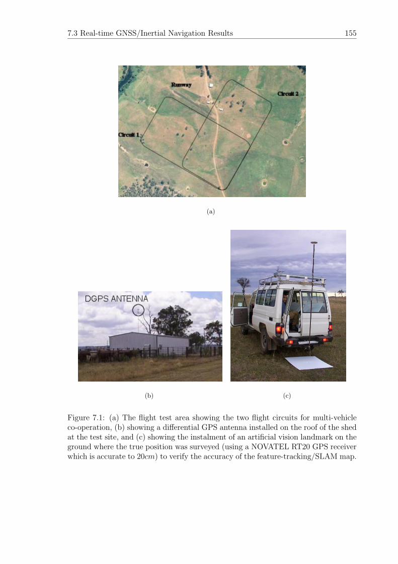
7.3 Real-time GNSS/Inertial Navigation Results 155
(a)
(b) (c)
Figure 7.1: (a) The flight test area showing the two flight circuits for multi-vehicleco-operation, (b) showing a differential GPS antenna installed on the roof of the shedat the test site, and (c) showing the instalment of an artificial vision landmark on theground where the true position was surveyed (using a NOVATEL RT20 GPS receiverwhich is accurate to 20cm) to verify the accuracy of the feature-tracking/SLAM map.
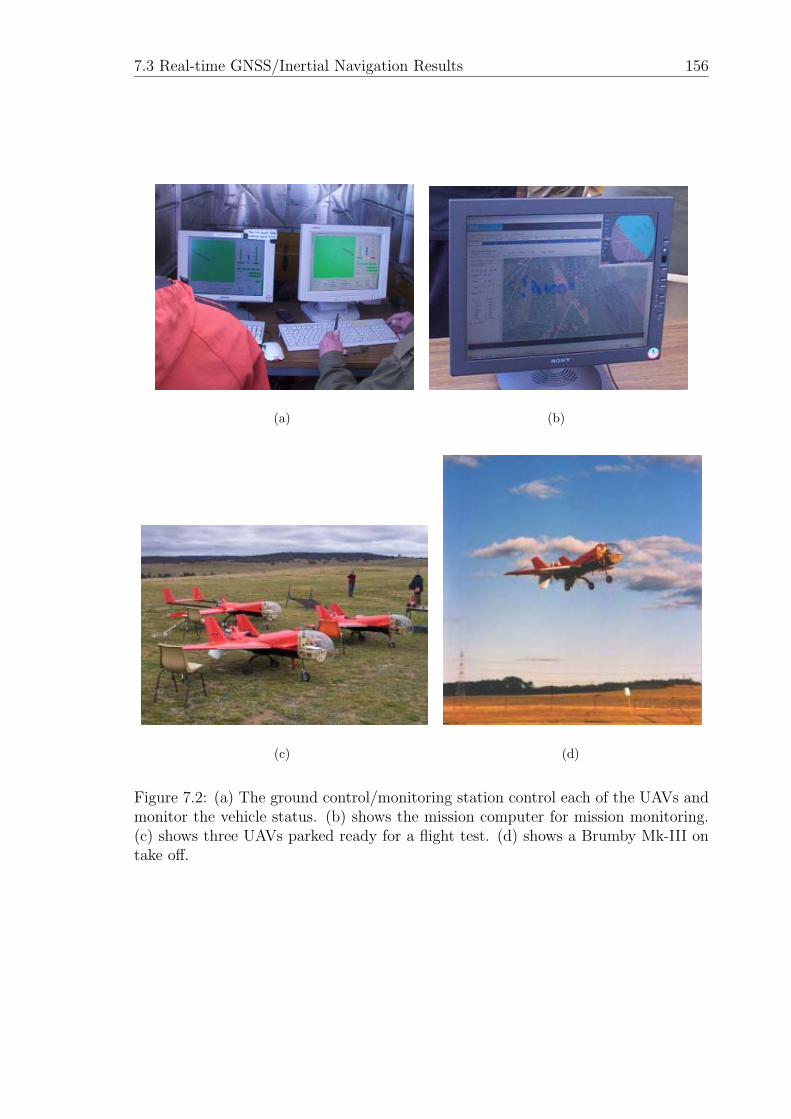
7.3 Real-time GNSS/Inertial Navigation Results 156
(a) (b)
(c) (d)
Figure 7.2: (a) The ground control/monitoring station control each of the UAVs andmonitor the vehicle status. (b) shows the mission computer for mission monitoring.(c) shows three UAVs parked ready for a flight test. (d) shows a Brumby Mk-III ontake off.
7.3 Real-time GNSS/Inertial Navigation Results 157
guidance and control loop as well as to the vision node for use in feature registration.
The visibility of GPS Satellite Vehicles (SV) varied from 4 to 8 during flight. The
maximum bank angle was limited to 60◦, which was required to meet the mission
profile. This steep banking typically caused the number of SVs to drop to 4 as can
be seen in Figure 7.5(a). Hence no significant error in GPS height was not observed.
Figure 7.3 presents the trajectory of a UAV on circuit-1 plotted with the GPS
position for comparison. The landmarks were installed under circuit-1 and circuit-2.
Figure 7.4 shows the 3D trajectory from the GNSS/Inertial system. Figure 7.5(b)
presents the GPS Figure Of Merit (FOM) data reported from the GPS receiver. The
FOM values are used as the strength of the measurement noise in the GNSS/Inertial
integration filter.
The autonomous flight trajectory is shown in more detail in Figures 7.6, 7.7, and
7.8. The vehicle took off in remote control mode and then put into loiter mode. After
one round, autonomous mode was activated and the vehicle underwent autonomous
control using way-point information uploaded before the flight. Different sets of
way-points were tried which imposed different flight trajectories. In this flight test
there were two particular trajectories sought after. The first was a benign race track
trajectory where the bank angles were kept to a minimum. In the second part of
the flight trial the vehicle was commanded to undertake more aggressive maneuvers.
After the mission completion the vehicle is commanded back to remote control mode
for landing.
The height is reported in the WGS-84 system which defines the height above the
ellipsoidal surface of the Earth. Figure 7.9 shows the vehicle height during manual
control and autonomous mode under benign flight conditions. Figure 7.10 presents
the height under the second component of the flight trial. It can be seen that the
GPS height is worse in the second component when compared to the first, due to the
frequent sharp bankings. In the following section it will be shown how these errors
can be minimised when using baro-altimeter aiding.
Figures 7.11 and 7.12 present the filter innovations computed on-line. The filter
7.3 Real-time GNSS/Inertial Navigation Results 158
innovations along the horizontal axes show some correlated dynamics which result
from the use of GPS velocity which is delayed and correlated to the position informa-
tion. This makes the filter tuning difficult due to its unknown covariance structure.
In fact it can be shown that in such situations position only information will pro-
vide similar results. The purpose of using velocity information here is because of the
constraints in the software structure which is designed to implement position and
velocity information from separate uncorrelated sources.
Figures 7.13, 7.14, and 7.15 show the estimated filter error state with its 1σ
uncertainty. In the error state filter configuration, the predicted state becomes zero
and the updated state is just the weighted innovation which means the error state
and innovation will show similar transition patterns. An important aspect in the
GNSS/Inertial system is the attitude error state which is estimated indirectly from the
velocity error. From Figure 7.15, the quality of the estimated attitude error, typically
the heading error, is dependent on vehicle dynamics [45]. In stationary conditions,
the heading uncertainty increases which means the heading is not observable from
the position/velocity observation. As soon as the vehicle moves, the heading error
becomes observable and the covariance decreases rapidly. This also happens during
flight, that is, under straight and level flight when no acceleration is experienced,
the heading uncertainty increases and any banking or acceleration in turn causes the
heading uncertainty to decrease as it becomes observable. In the following chapter
further insight into the observability of such systems will be discussed.
Figures 7.16 and 7.17 depict the raw IMU data measured in the body frame. From
the plots, the Y and Z acceleration show greater values than the X axis acceleration
due to the excessive rolling motions which introduce gravity acceleration in the Y
and Z axes. The structure of the engine which has a vertical piston also introduces
more vibration noise in these axes. Figure 7.18 and 7.19 presents the power spectral
density for the angular velocity along the X axis. The engine vibration can be clearly
observed from the high frequency region at around 110Hz (6600RPM). The impacts
during take off and landing can also be seen from the constant level of energy (or
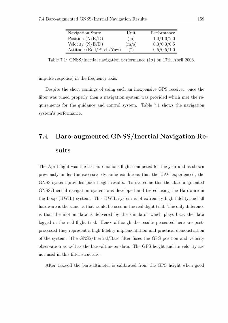
7.4 Baro-augmented GNSS/Inertial Navigation Results 159
Navigation State Unit PerformancePosition (N/E/D) (m) 1.0/1.0/2.0Velocity (N/E/D) (m/s) 0.3/0.3/0.5Attitude (Roll/Pitch/Yaw) (◦) 0.5/0.5/1.0
Table 7.1: GNSS/Inertial navigation performance (1σ) on 17th April 2003.
impulse response) in the frequency axis.
Despite the short comings of using such an inexpensive GPS receiver, once the
filter was tuned properly then a navigation system was provided which met the re-
quirements for the guidance and control system. Table 7.1 shows the navigation
system’s performance.
7.4 Baro-augmented GNSS/Inertial Navigation Re-
sults
The April flight was the last autonomous flight conducted for the year and as shown
previously under the excessive dynamic conditions that the UAV experienced, the
GNSS system provided poor height results. To overcome this the Baro-augmented
GNSS/Inertial navigation system was developed and tested using the Hardware in
the Loop (HWIL) system. This HWIL system is of extremely high fidelity and all
hardware is the same as that would be used in the real flight trial. The only difference
is that the motion data is delivered by the simulator which plays back the data
logged in the real flight trial. Hence although the results presented here are post-
processed they represent a high fidelity implementation and practical demonstration
of the system. The GNSS/Inertial/Baro filter fuses the GPS position and velocity
observation as well as the baro-altimeter data. The GPS height and its velocity are
not used in this filter structure.
After take-off the baro-altimeter is calibrated from the GPS height when good
7.4 Baro-augmented GNSS/Inertial Navigation Results 160
VDOP is available. Then the baro-altimeter is used for vertical aiding while the GPS
data is used for horizontal aiding. Figure 7.20 shows the estimated 2D trajectory
which shows similar performance to the GNSS/Inertial horizontal trajectory. Figures
7.21 to 7.24 compare the estimated height between the GNSS/Inertial/Baro filter
and the GNSS/Inertial filter under the same flight conditions presented in the previ-
ous section. Figure 7.21 shows the height during taking-off and climbing where the
baro-altimeter shows some overshoot. Figure 7.22 shows additional height error in
the baro-altitude which occurred during the autonomous mode flight. Whenever the
vehicle descends rapidly, the baro-altimeter shows some errors. The reason is not
clear, however the pressure sensors on the fuselage seemed not to be firmly attached,
hence they could be affected by the vehicle dynamics and internal air flow. However,
the improvement of baro aiding can be seen clearly in Figure 7.23 where the vehicle
underwent excessive banking and introduced errors in the GNSS altitude solution
during autonomous flight. The baro-aided GNSS/Inertial solution showed more reli-
able results then when compared to the non-Baro aided system. Figure 7.24 presents
the height data during landing where the baro-altimeter, and GNSS/Inertial/Baro as
well, show some drift compared to the GPS height because the baro-altimeter was
initialised only at the beginning of the flight. This drift however, can be overcame
by periodically resetting the baro-altimeter by using the GNSS height whenever it is
under good quality.
In conclusion, as there were more than four satellites in this flight trial, no signifi-
cant errors in GPS height occurred under the benign flight condition. During this pe-
riod the GNSS/Inertial/Baro showed a comparable performance to the GNSS/Inertial
navigation. However during sharp banking periods, the GNSS/Inertial/Baro fil-
ter provided much smoother and more reliable results compared to those of the
GNSS/Inertial.
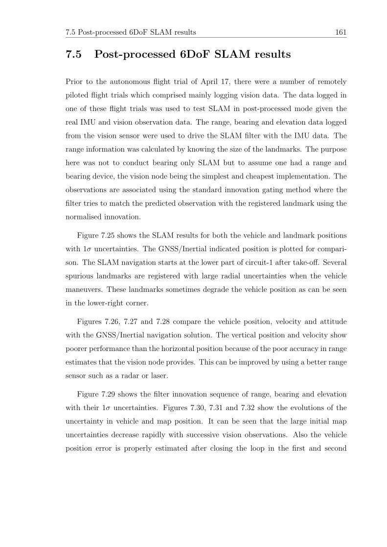
7.5 Post-processed 6DoF SLAM results 161
7.5 Post-processed 6DoF SLAM results
Prior to the autonomous flight trial of April 17, there were a number of remotely
piloted flight trials which comprised mainly logging vision data. The data logged in
one of these flight trials was used to test SLAM in post-processed mode given the
real IMU and vision observation data. The range, bearing and elevation data logged
from the vision sensor were used to drive the SLAM filter with the IMU data. The
range information was calculated by knowing the size of the landmarks. The purpose
here was not to conduct bearing only SLAM but to assume one had a range and
bearing device, the vision node being the simplest and cheapest implementation. The
observations are associated using the standard innovation gating method where the
filter tries to match the predicted observation with the registered landmark using the
normalised innovation.
Figure 7.25 shows the SLAM results for both the vehicle and landmark positions
with 1σ uncertainties. The GNSS/Inertial indicated position is plotted for compari-
son. The SLAM navigation starts at the lower part of circuit-1 after take-off. Several
spurious landmarks are registered with large radial uncertainties when the vehicle
maneuvers. These landmarks sometimes degrade the vehicle position as can be seen
in the lower-right corner.
Figures 7.26, 7.27 and 7.28 compare the vehicle position, velocity and attitude
with the GNSS/Inertial navigation solution. The vertical position and velocity show
poorer performance than the horizontal position because of the poor accuracy in range
estimates that the vision node provides. This can be improved by using a better range
sensor such as a radar or laser.
Figure 7.29 shows the filter innovation sequence of range, bearing and elevation
with their 1σ uncertainties. Figures 7.30, 7.31 and 7.32 show the evolutions of the
uncertainty in vehicle and map position. It can be seen that the large initial map
uncertainties decrease rapidly with successive vision observations. Also the vehicle
position error is properly estimated after closing the loop in the first and second
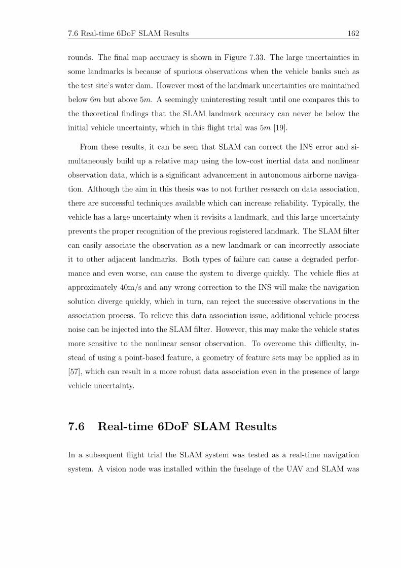
7.6 Real-time 6DoF SLAM Results 162
rounds. The final map accuracy is shown in Figure 7.33. The large uncertainties in
some landmarks is because of spurious observations when the vehicle banks such as
the test site’s water dam. However most of the landmark uncertainties are maintained
below 6m but above 5m. A seemingly uninteresting result until one compares this to
the theoretical findings that the SLAM landmark accuracy can never be below the
initial vehicle uncertainty, which in this flight trial was 5m [19].
From these results, it can be seen that SLAM can correct the INS error and si-
multaneously build up a relative map using the low-cost inertial data and nonlinear
observation data, which is a significant advancement in autonomous airborne naviga-
tion. Although the aim in this thesis was to not further research on data association,
there are successful techniques available which can increase reliability. Typically, the
vehicle has a large uncertainty when it revisits a landmark, and this large uncertainty
prevents the proper recognition of the previous registered landmark. The SLAM filter
can easily associate the observation as a new landmark or can incorrectly associate
it to other adjacent landmarks. Both types of failure can cause a degraded perfor-
mance and even worse, can cause the system to diverge quickly. The vehicle flies at
approximately 40m/s and any wrong correction to the INS will make the navigation
solution diverge quickly, which in turn, can reject the successive observations in the
association process. To relieve this data association issue, additional vehicle process
noise can be injected into the SLAM filter. However, this may make the vehicle states
more sensitive to the nonlinear sensor observation. To overcome this difficulty, in-
stead of using a point-based feature, a geometry of feature sets may be applied as in
[57], which can result in a more robust data association even in the presence of large
vehicle uncertainty.
7.6 Real-time 6DoF SLAM Results
In a subsequent flight trial the SLAM system was tested as a real-time navigation
system. A vision node was installed within the fuselage of the UAV and SLAM was
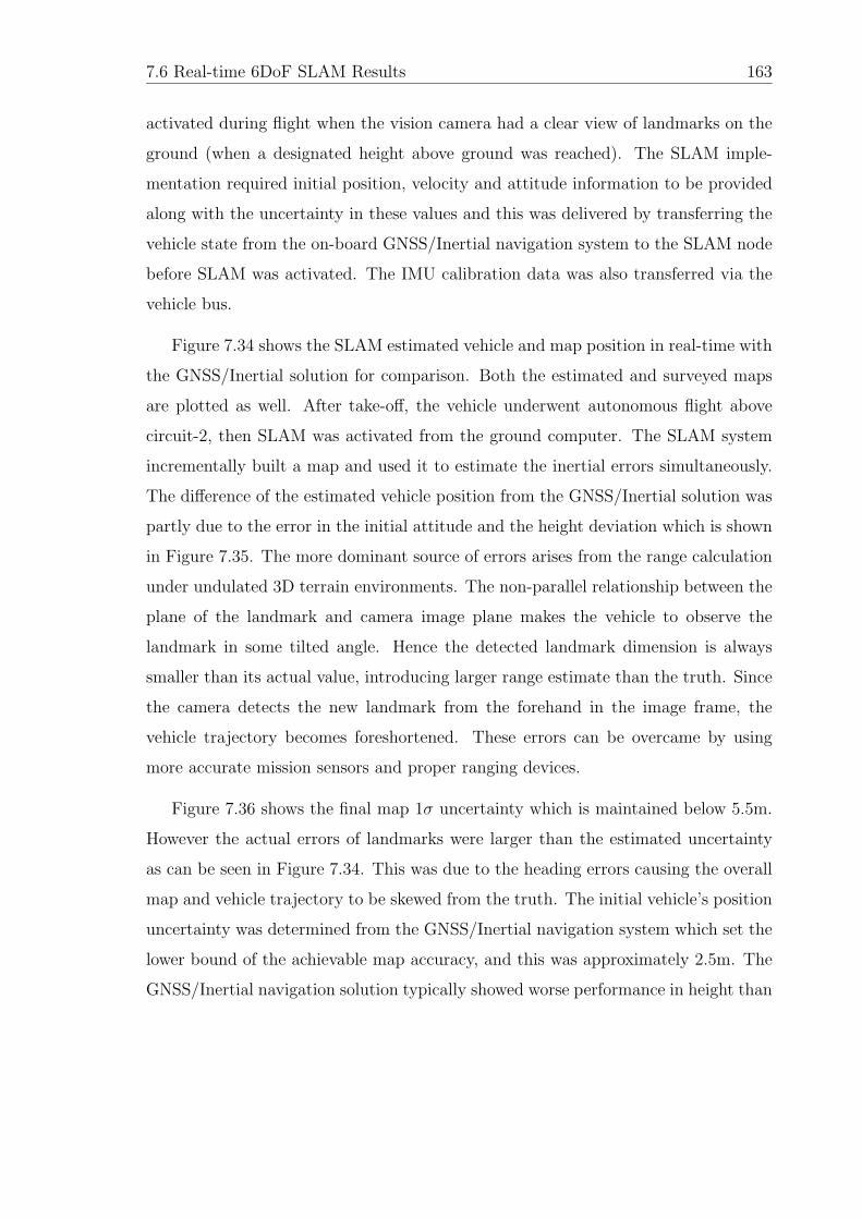
7.6 Real-time 6DoF SLAM Results 163
activated during flight when the vision camera had a clear view of landmarks on the
ground (when a designated height above ground was reached). The SLAM imple-
mentation required initial position, velocity and attitude information to be provided
along with the uncertainty in these values and this was delivered by transferring the
vehicle state from the on-board GNSS/Inertial navigation system to the SLAM node
before SLAM was activated. The IMU calibration data was also transferred via the
vehicle bus.
Figure 7.34 shows the SLAM estimated vehicle and map position in real-time with
the GNSS/Inertial solution for comparison. Both the estimated and surveyed maps
are plotted as well. After take-off, the vehicle underwent autonomous flight above
circuit-2, then SLAM was activated from the ground computer. The SLAM system
incrementally built a map and used it to estimate the inertial errors simultaneously.
The difference of the estimated vehicle position from the GNSS/Inertial solution was
partly due to the error in the initial attitude and the height deviation which is shown
in Figure 7.35. The more dominant source of errors arises from the range calculation
under undulated 3D terrain environments. The non-parallel relationship between the
plane of the landmark and camera image plane makes the vehicle to observe the
landmark in some tilted angle. Hence the detected landmark dimension is always
smaller than its actual value, introducing larger range estimate than the truth. Since
the camera detects the new landmark from the forehand in the image frame, the
vehicle trajectory becomes foreshortened. These errors can be overcame by using
more accurate mission sensors and proper ranging devices.
Figure 7.36 shows the final map 1σ uncertainty which is maintained below 5.5m.
However the actual errors of landmarks were larger than the estimated uncertainty
as can be seen in Figure 7.34. This was due to the heading errors causing the overall
map and vehicle trajectory to be skewed from the truth. The initial vehicle’s position
uncertainty was determined from the GNSS/Inertial navigation system which set the
lower bound of the achievable map accuracy, and this was approximately 2.5m. The
GNSS/Inertial navigation solution typically showed worse performance in height than
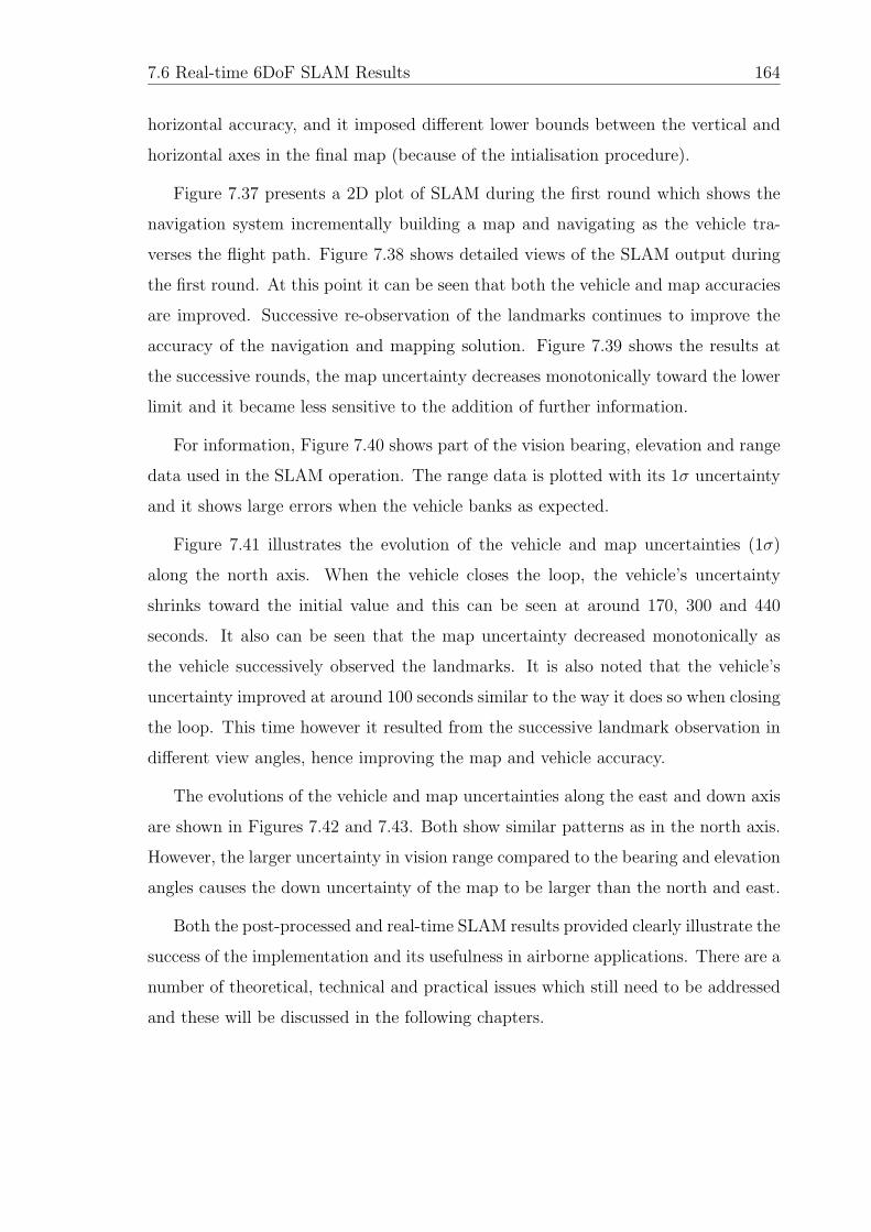
7.6 Real-time 6DoF SLAM Results 164
horizontal accuracy, and it imposed different lower bounds between the vertical and
horizontal axes in the final map (because of the intialisation procedure).
Figure 7.37 presents a 2D plot of SLAM during the first round which shows the
navigation system incrementally building a map and navigating as the vehicle tra-
verses the flight path. Figure 7.38 shows detailed views of the SLAM output during
the first round. At this point it can be seen that both the vehicle and map accuracies
are improved. Successive re-observation of the landmarks continues to improve the
accuracy of the navigation and mapping solution. Figure 7.39 shows the results at
the successive rounds, the map uncertainty decreases monotonically toward the lower
limit and it became less sensitive to the addition of further information.
For information, Figure 7.40 shows part of the vision bearing, elevation and range
data used in the SLAM operation. The range data is plotted with its 1σ uncertainty
and it shows large errors when the vehicle banks as expected.
Figure 7.41 illustrates the evolution of the vehicle and map uncertainties (1σ)
along the north axis. When the vehicle closes the loop, the vehicle’s uncertainty
shrinks toward the initial value and this can be seen at around 170, 300 and 440
seconds. It also can be seen that the map uncertainty decreased monotonically as
the vehicle successively observed the landmarks. It is also noted that the vehicle’s
uncertainty improved at around 100 seconds similar to the way it does so when closing
the loop. This time however it resulted from the successive landmark observation in
different view angles, hence improving the map and vehicle accuracy.
The evolutions of the vehicle and map uncertainties along the east and down axis
are shown in Figures 7.42 and 7.43. Both show similar patterns as in the north axis.
However, the larger uncertainty in vision range compared to the bearing and elevation
angles causes the down uncertainty of the map to be larger than the north and east.
Both the post-processed and real-time SLAM results provided clearly illustrate the
success of the implementation and its usefulness in airborne applications. There are a
number of theoretical, technical and practical issues which still need to be addressed
and these will be discussed in the following chapters.
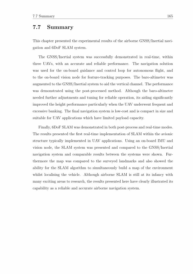
7.7 Summary 165
7.7 Summary
This chapter presented the experimental results of the airborne GNSS/Inertial navi-
gation and 6DoF SLAM system.
The GNSS/Inertial system was successfully demonstrated in real-time, within
three UAVs, with an accurate and reliable performance. The navigation solution
was used for the on-board guidance and control loop for autonomous flight, and
to the on-board vision node for feature-tracking purposes. The baro-altimeter was
augmented to the GNSS/Inertial system to aid the vertical channel. The performance
was demonstrated using the post-processed method. Although the baro-altimeter
needed further adjustments and tuning for reliable operation, its aiding significantly
improved the height performance particularly when the UAV underwent frequent and
excessive banking. The final navigation system is low-cost and is compact in size and
suitable for UAV applications which have limited payload capacity.
Finally, 6DoF SLAM was demonstrated in both post-process and real-time modes.
The results presented the first real-time implementation of SLAM within the avionic
structure typically implemented in UAV applications. Using an on-board IMU and
vision node, the SLAM system was presented and compared to the GNSS/Inertial
navigation system and comparable results between the systems were shown. Fur-
thermore the map was compared to the surveyed landmarks and also showed the
ability for the SLAM algorithm to simultaneously build a map of the environment
whilst localising the vehicle. Although airborne SLAM is still at its infancy with
many exciting areas to research, the results presented here have clearly illustrated its
capability as a reliable and accurate airborne navigation system.
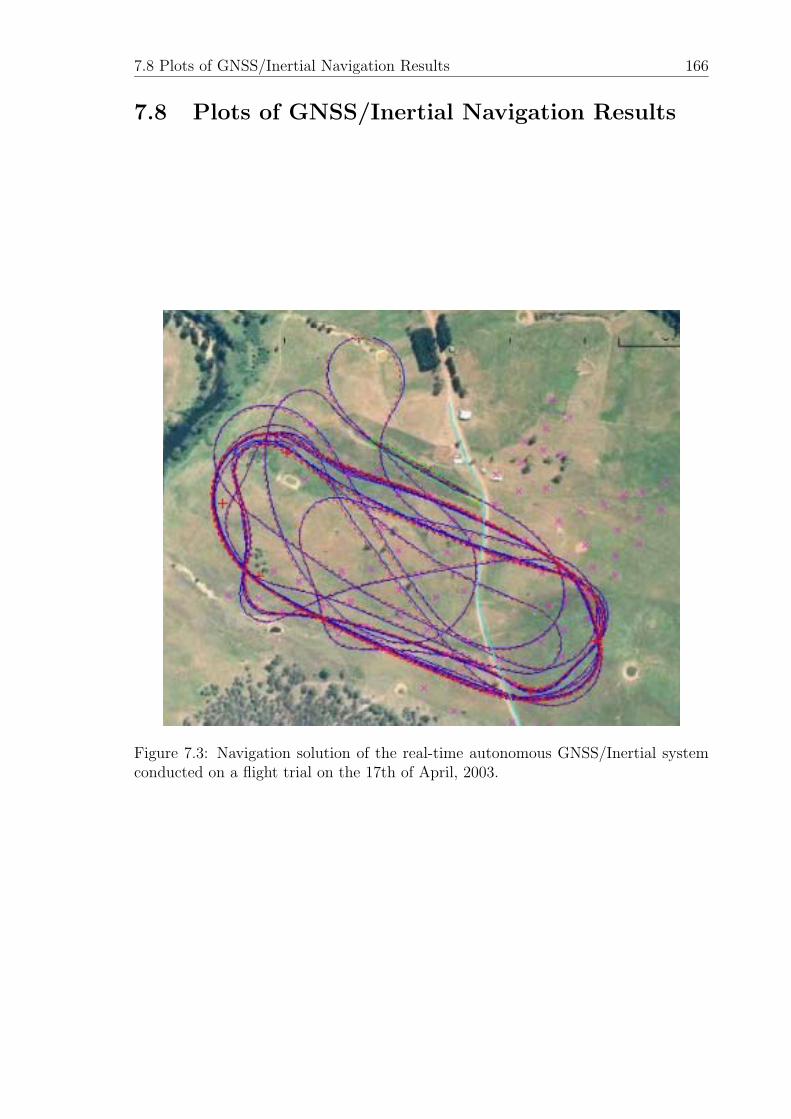
7.8 Plots of GNSS/Inertial Navigation Results 166
7.8 Plots of GNSS/Inertial Navigation Results
Figure 7.3: Navigation solution of the real-time autonomous GNSS/Inertial systemconducted on a flight trial on the 17th of April, 2003.
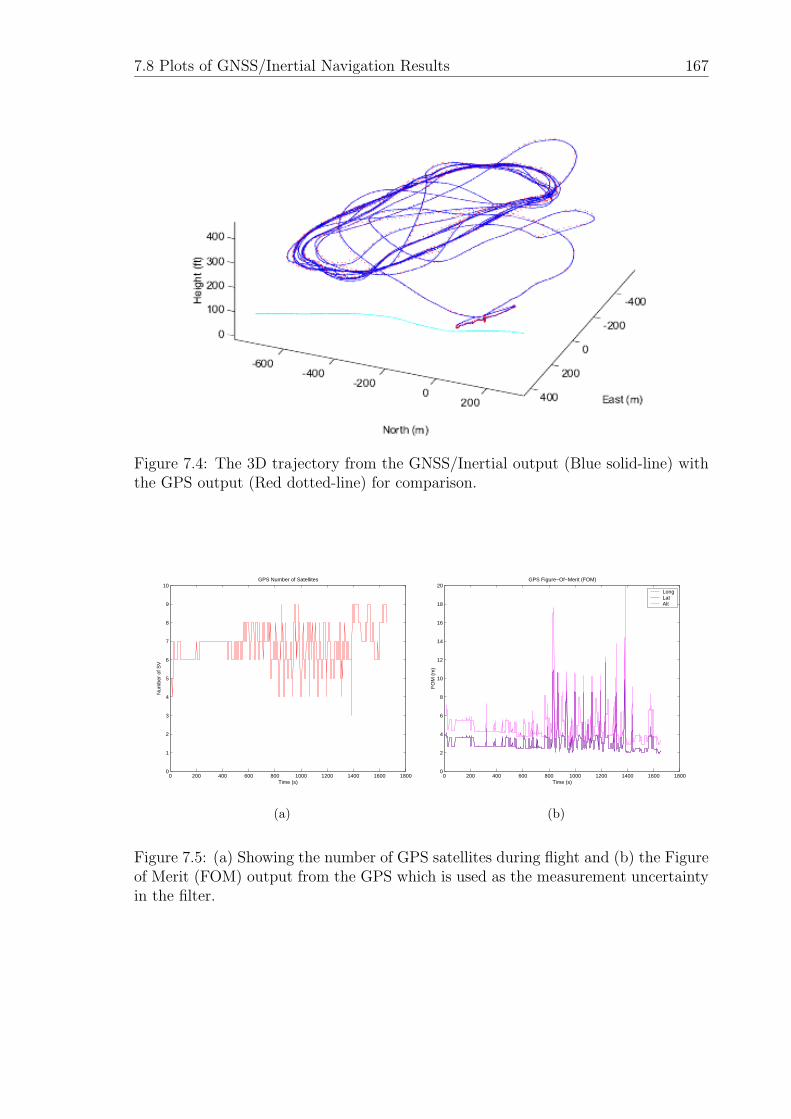
7.8 Plots of GNSS/Inertial Navigation Results 167
Figure 7.4: The 3D trajectory from the GNSS/Inertial output (Blue solid-line) withthe GPS output (Red dotted-line) for comparison.
0 200 400 600 800 1000 1200 1400 1600 18000
1
2
3
4
5
6
7
8
9
10GPS Number of Satellites
Num
ber
of S
V
Time (s)
(a)
0 200 400 600 800 1000 1200 1400 1600 18000
2
4
6
8
10
12
14
16
18
20GPS Figure−Of−Merit (FOM)
Time (s)
FO
M (
m)
LongLatAlt
(b)
Figure 7.5: (a) Showing the number of GPS satellites during flight and (b) the Figureof Merit (FOM) output from the GPS which is used as the measurement uncertaintyin the filter.
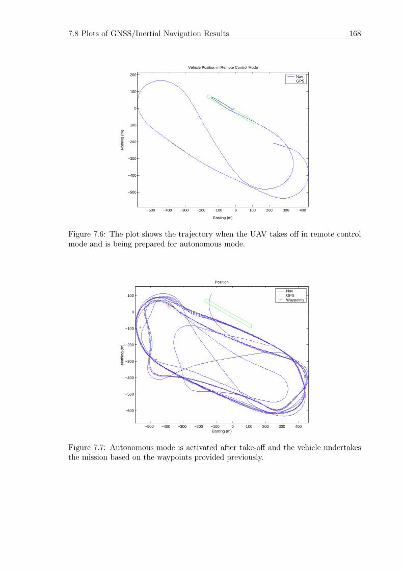
7.8 Plots of GNSS/Inertial Navigation Results 168
−500 −400 −300 −200 −100 0 100 200 300 400
−500
−400
−300
−200
−100
0
100
200
Vehicle Position in Remote Control Mode
Not
hing
(m
)
Easting (m)
NavGPS
Figure 7.6: The plot shows the trajectory when the UAV takes off in remote controlmode and is being prepared for autonomous mode.
−500 −400 −300 −200 −100 0 100 200 300 400
−600
−500
−400
−300
−200
−100
0
100
Position
Not
hing
(m
)
Easting (m)
NavGPSWaypoints
Figure 7.7: Autonomous mode is activated after take-off and the vehicle undertakesthe mission based on the waypoints provided previously.
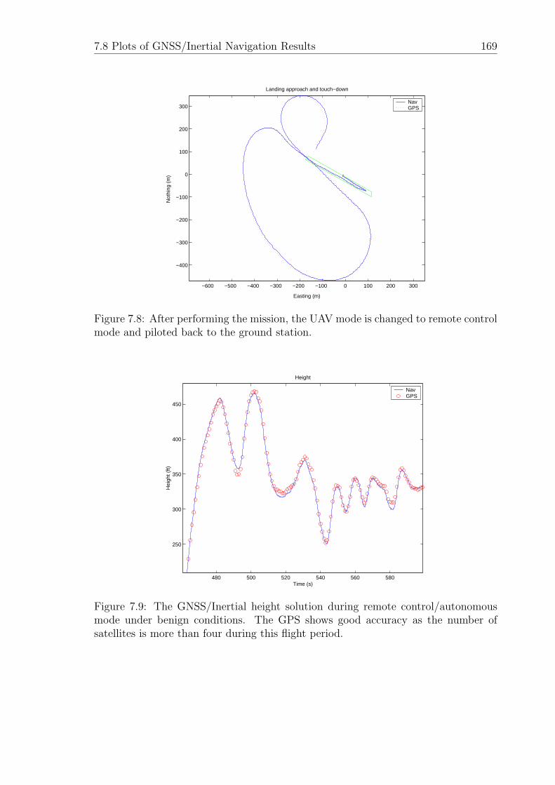
7.8 Plots of GNSS/Inertial Navigation Results 169
−600 −500 −400 −300 −200 −100 0 100 200 300
−400
−300
−200
−100
0
100
200
300
Landing approach and touch−down
Not
hing
(m
)
Easting (m)
NavGPS
Figure 7.8: After performing the mission, the UAV mode is changed to remote controlmode and piloted back to the ground station.
480 500 520 540 560 580
250
300
350
400
450
Height
Hei
ght (
ft)
Time (s)
NavGPS
Figure 7.9: The GNSS/Inertial height solution during remote control/autonomousmode under benign conditions. The GPS shows good accuracy as the number ofsatellites is more than four during this flight period.
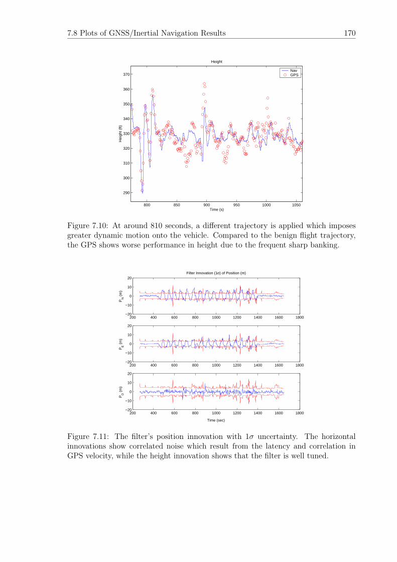
7.8 Plots of GNSS/Inertial Navigation Results 170
800 850 900 950 1000 1050
290
300
310
320
330
340
350
360
370
Height
Hei
ght (
ft)
Time (s)
NavGPS
Figure 7.10: At around 810 seconds, a different trajectory is applied which imposesgreater dynamic motion onto the vehicle. Compared to the benign flight trajectory,the GPS shows worse performance in height due to the frequent sharp banking.
200 400 600 800 1000 1200 1400 1600 1800−20
−10
0
10
20Filter Innovation (1σ) of Position (m)
PN
(m
)
200 400 600 800 1000 1200 1400 1600 1800−20
−10
0
10
20
PE (
m)
200 400 600 800 1000 1200 1400 1600 1800−20
−10
0
10
20
PD
(m
)
Time (sec)
Figure 7.11: The filter’s position innovation with 1σ uncertainty. The horizontalinnovations show correlated noise which result from the latency and correlation inGPS velocity, while the height innovation shows that the filter is well tuned.
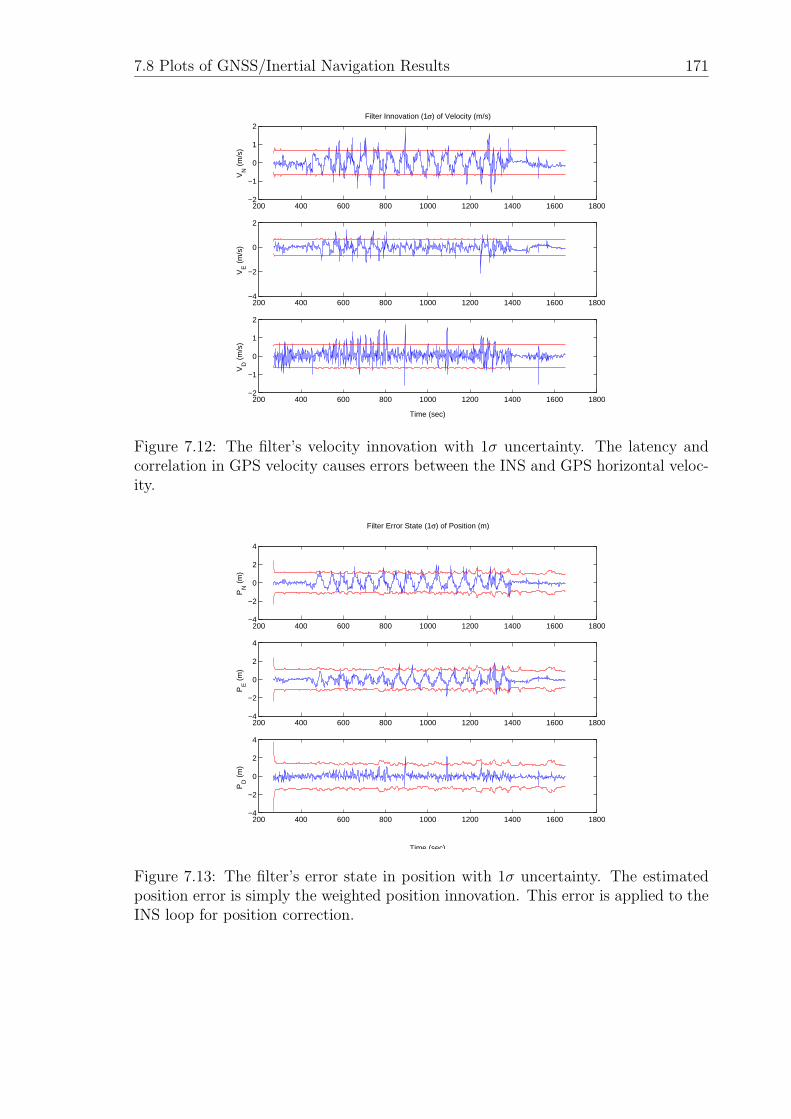
7.8 Plots of GNSS/Inertial Navigation Results 171
200 400 600 800 1000 1200 1400 1600 1800−2
−1
0
1
2Filter Innovation (1σ) of Velocity (m/s)
VN
(m
/s)
200 400 600 800 1000 1200 1400 1600 1800−4
−2
0
2
VE (
m/s
)
200 400 600 800 1000 1200 1400 1600 1800−2
−1
0
1
2
VD
(m
/s)
Time (sec)
Figure 7.12: The filter’s velocity innovation with 1σ uncertainty. The latency andcorrelation in GPS velocity causes errors between the INS and GPS horizontal veloc-ity.
200 400 600 800 1000 1200 1400 1600 1800−4
−2
0
2
4
Filter Error State (1σ) of Position (m)
PN
(m
)
200 400 600 800 1000 1200 1400 1600 1800−4
−2
0
2
4
PE (
m)
200 400 600 800 1000 1200 1400 1600 1800−4
−2
0
2
4
PD
(m
)
Time (sec)
Figure 7.13: The filter’s error state in position with 1σ uncertainty. The estimatedposition error is simply the weighted position innovation. This error is applied to theINS loop for position correction.
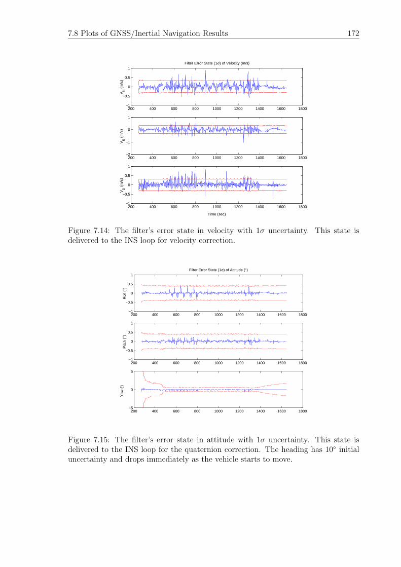
7.8 Plots of GNSS/Inertial Navigation Results 172
200 400 600 800 1000 1200 1400 1600 1800−1
−0.5
0
0.5
1Filter Error State (1σ) of Velocity (m/s)
VN
(m
/s)
200 400 600 800 1000 1200 1400 1600 1800−2
−1
0
1V
E (
m/s
)
200 400 600 800 1000 1200 1400 1600 1800−1
−0.5
0
0.5
1
VD
(m
/s)
Time (sec)
Figure 7.14: The filter’s error state in velocity with 1σ uncertainty. This state isdelivered to the INS loop for velocity correction.
200 400 600 800 1000 1200 1400 1600 1800−1
−0.5
0
0.5
1Filter Error State (1σ) of Attitude (°)
Rol
l (°)
200 400 600 800 1000 1200 1400 1600 1800−1
−0.5
0
0.5
1
Pitc
h (°
)
200 400 600 800 1000 1200 1400 1600 1800−5
0
5
Yaw
(°)
Figure 7.15: The filter’s error state in attitude with 1σ uncertainty. This state isdelivered to the INS loop for the quaternion correction. The heading has 10◦ initialuncertainty and drops immediately as the vehicle starts to move.
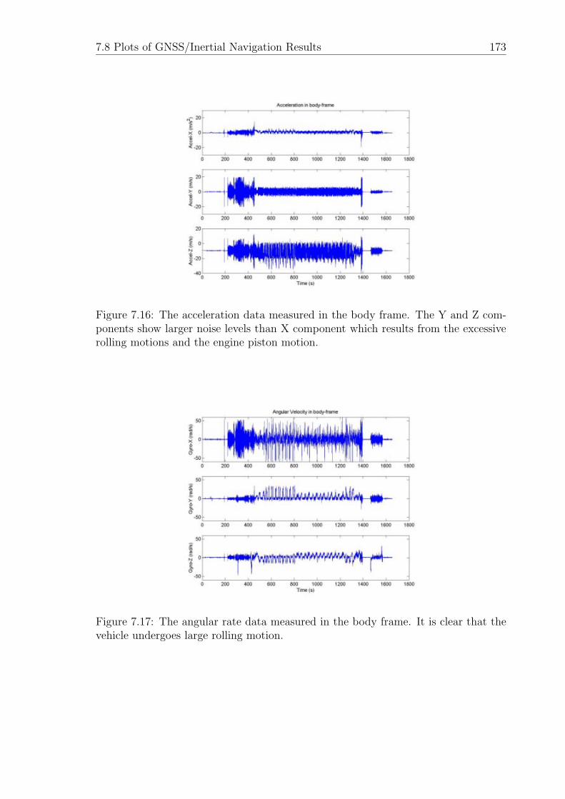
7.8 Plots of GNSS/Inertial Navigation Results 173
Figure 7.16: The acceleration data measured in the body frame. The Y and Z com-ponents show larger noise levels than X component which results from the excessiverolling motions and the engine piston motion.
Figure 7.17: The angular rate data measured in the body frame. It is clear that thevehicle undergoes large rolling motion.
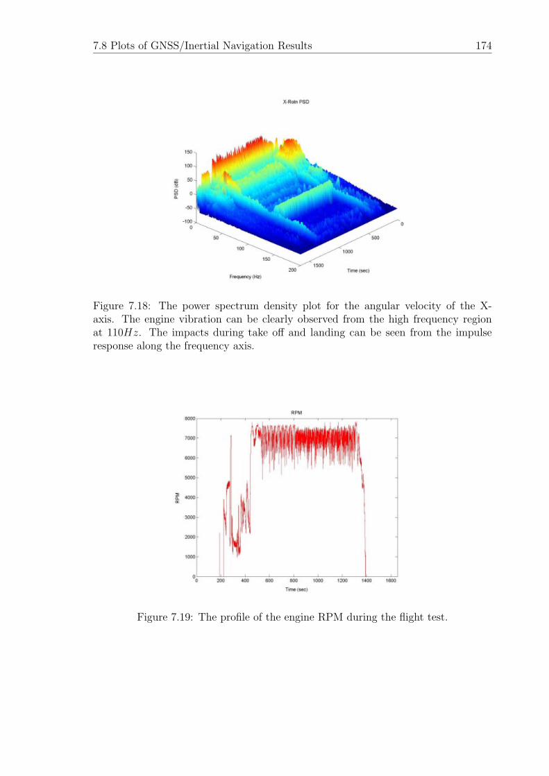
7.8 Plots of GNSS/Inertial Navigation Results 174
Figure 7.18: The power spectrum density plot for the angular velocity of the X-axis. The engine vibration can be clearly observed from the high frequency regionat 110Hz. The impacts during take off and landing can be seen from the impulseresponse along the frequency axis.
Figure 7.19: The profile of the engine RPM during the flight test.
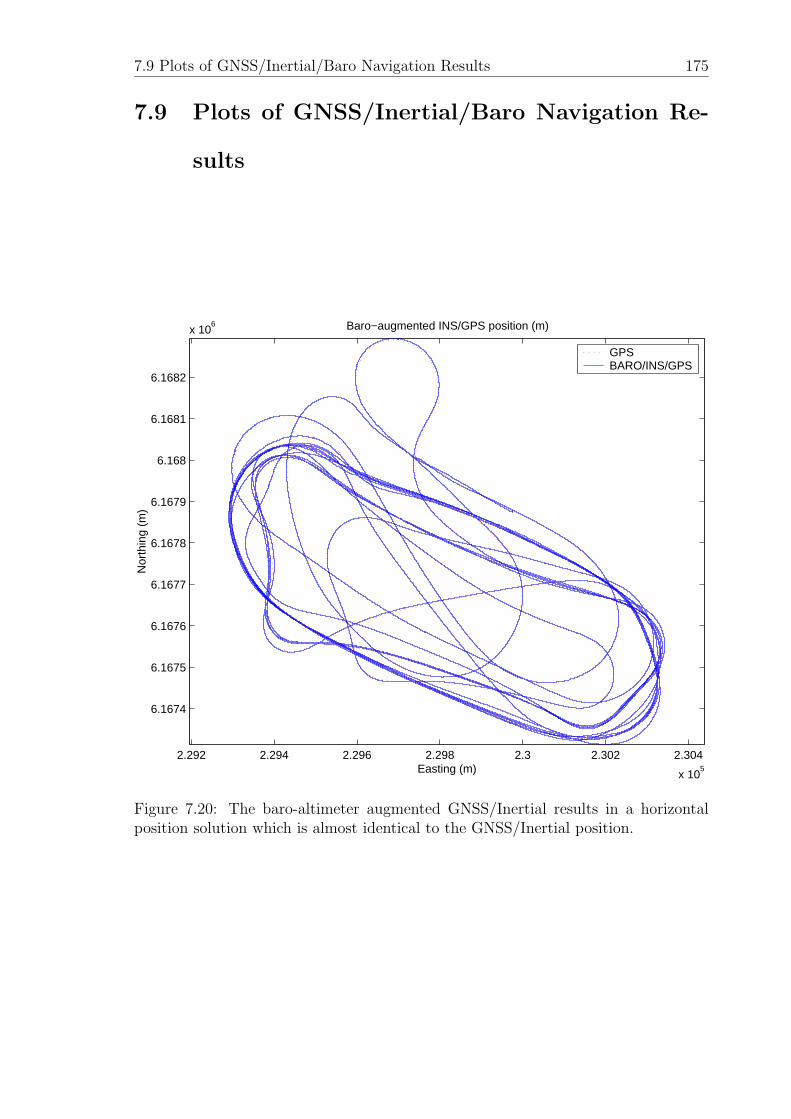
7.9 Plots of GNSS/Inertial/Baro Navigation Results 175
7.9 Plots of GNSS/Inertial/Baro Navigation Re-
sults
2.292 2.294 2.296 2.298 2.3 2.302 2.304
x 105
6.1674
6.1675
6.1676
6.1677
6.1678
6.1679
6.168
6.1681
6.1682
x 106
Easting (m)
Nor
thin
g (m
)
Baro−augmented INS/GPS position (m)
GPSBARO/INS/GPS
Figure 7.20: The baro-altimeter augmented GNSS/Inertial results in a horizontalposition solution which is almost identical to the GNSS/Inertial position.
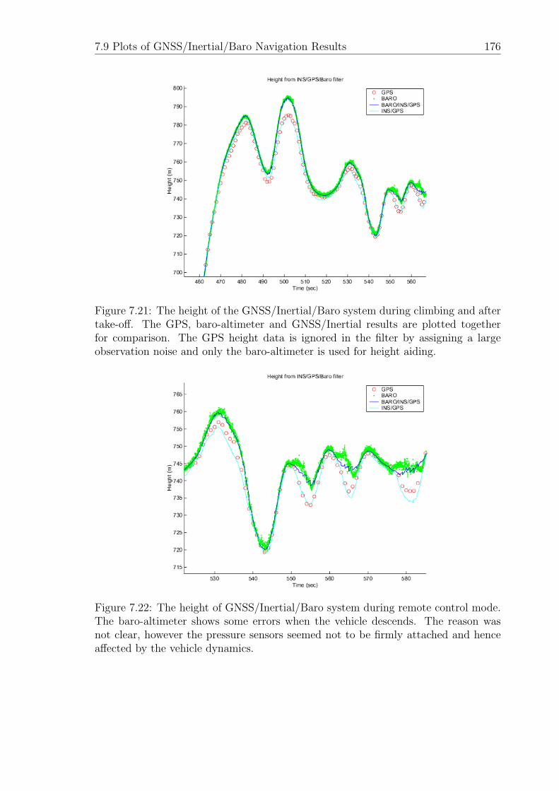
7.9 Plots of GNSS/Inertial/Baro Navigation Results 176
Figure 7.21: The height of the GNSS/Inertial/Baro system during climbing and aftertake-off. The GPS, baro-altimeter and GNSS/Inertial results are plotted togetherfor comparison. The GPS height data is ignored in the filter by assigning a largeobservation noise and only the baro-altimeter is used for height aiding.
Figure 7.22: The height of GNSS/Inertial/Baro system during remote control mode.The baro-altimeter shows some errors when the vehicle descends. The reason wasnot clear, however the pressure sensors seemed not to be firmly attached and henceaffected by the vehicle dynamics.
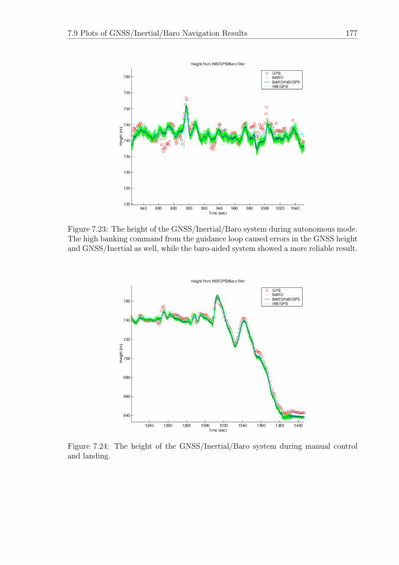
7.9 Plots of GNSS/Inertial/Baro Navigation Results 177
Figure 7.23: The height of the GNSS/Inertial/Baro system during autonomous mode.The high banking command from the guidance loop caused errors in the GNSS heightand GNSS/Inertial as well, while the baro-aided system showed a more reliable result.
Figure 7.24: The height of the GNSS/Inertial/Baro system during manual controland landing.
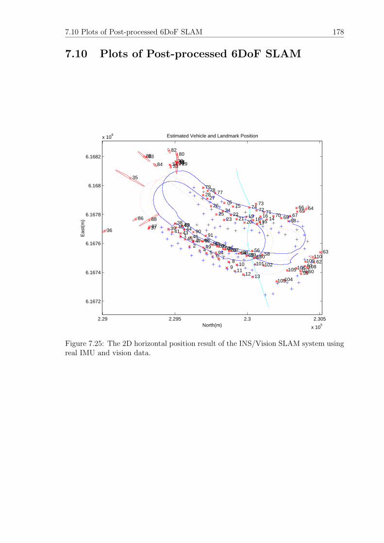
7.10 Plots of Post-processed 6DoF SLAM 178
7.10 Plots of Post-processed 6DoF SLAM
2.29 2.295 2.3 2.305
x 105
6.1672
6.1674
6.1676
6.1678
6.168
6.1682
x 106 Estimated Vehicle and Landmark Position
1
2 3
4 5 6 7
8 9
10 11
12 13
14 15 16
17 18
19 20
21 22
23
24 25
26
27 28
29 30 31 32
33 34
35
36 37 38
39 40 41
42
43 44
45 46 47 48
49 50 51 52 53 54 55
56 57
58
59 60 61
62
63
64 65 66
67 68
69 70 71 72
73 74 75
76
77 78 79
80
81
82 83
84
85
86
87
88 89
90 91
92 93
94 95 96 97 98 99100
101102
103104
105 106107108
109110
North(m)
Eas
t(m
)
Figure 7.25: The 2D horizontal position result of the INS/Vision SLAM system usingreal IMU and vision data.
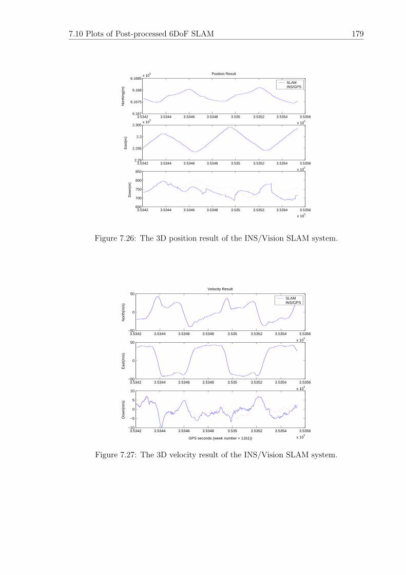
7.10 Plots of Post-processed 6DoF SLAM 179
3.5342 3.5344 3.5346 3.5348 3.535 3.5352 3.5354 3.5356
x 105
6.167
6.1675
6.168
6.1685x 10
6 Position Result
Nor
thin
g(m
)
SLAMINS/GPS
3.5342 3.5344 3.5346 3.5348 3.535 3.5352 3.5354 3.5356
x 105
2.29
2.295
2.3
2.305x 10
5
Eas
t(m
)
3.5342 3.5344 3.5346 3.5348 3.535 3.5352 3.5354 3.5356
x 105
650
700
750
800
850
Dow
n(m
)
Figure 7.26: The 3D position result of the INS/Vision SLAM system.
3.5342 3.5344 3.5346 3.5348 3.535 3.5352 3.5354 3.5356
x 105
−50
0
50Velocity Result
Nor
th(m
/s)
SLAMINS/GPS
3.5342 3.5344 3.5346 3.5348 3.535 3.5352 3.5354 3.5356
x 105
−50
0
50
Eas
t(m
/s)
3.5342 3.5344 3.5346 3.5348 3.535 3.5352 3.5354 3.5356
x 105
−10
−5
0
5
10
Dow
n(m
/s)
GPS seconds (week number = 1161))
Figure 7.27: The 3D velocity result of the INS/Vision SLAM system.
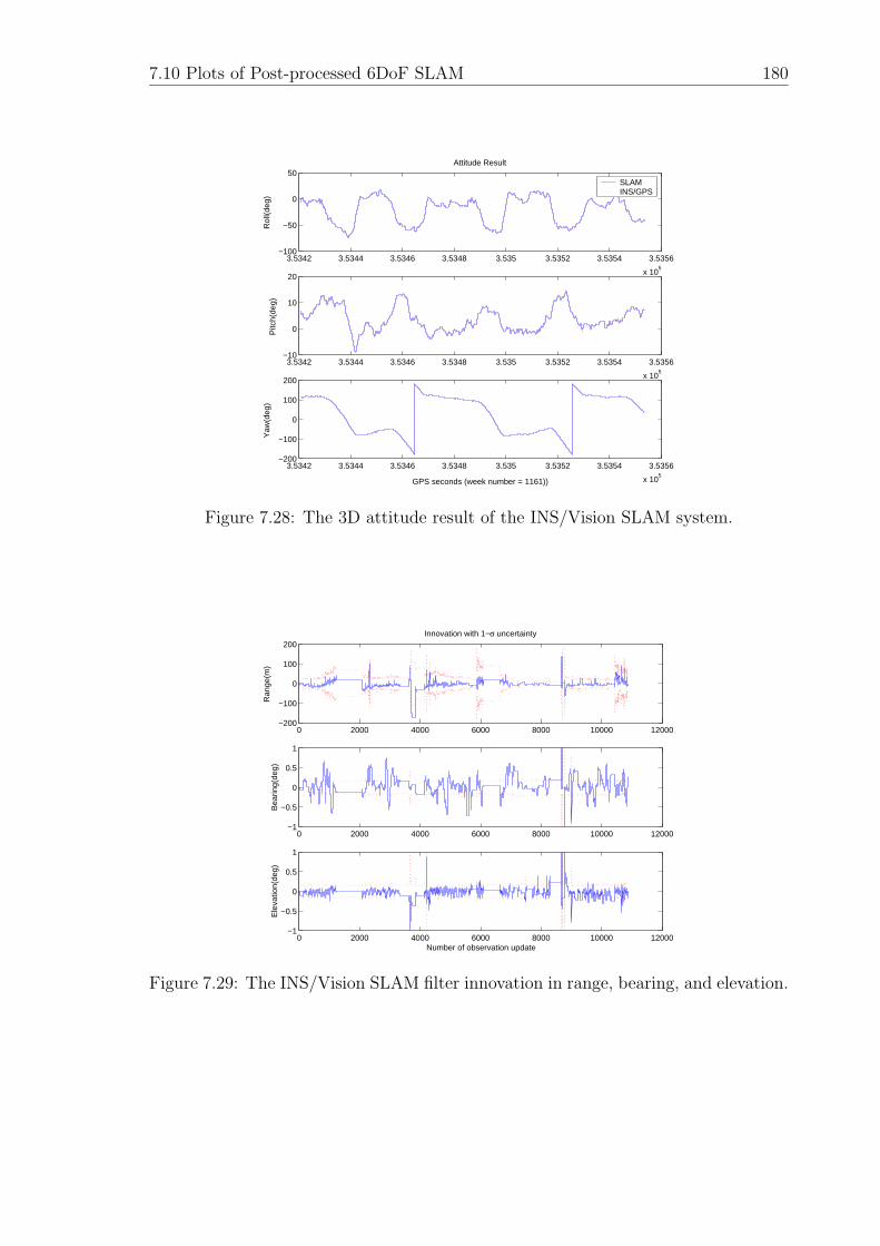
7.10 Plots of Post-processed 6DoF SLAM 180
3.5342 3.5344 3.5346 3.5348 3.535 3.5352 3.5354 3.5356
x 105
−100
−50
0
50Attitude Result
Rol
l(deg
)
SLAMINS/GPS
3.5342 3.5344 3.5346 3.5348 3.535 3.5352 3.5354 3.5356
x 105
−10
0
10
20P
itch(
deg)
3.5342 3.5344 3.5346 3.5348 3.535 3.5352 3.5354 3.5356
x 105
−200
−100
0
100
200
Yaw
(deg
)
GPS seconds (week number = 1161))
Figure 7.28: The 3D attitude result of the INS/Vision SLAM system.
0 2000 4000 6000 8000 10000 12000−200
−100
0
100
200Innovation with 1−σ uncertainty
Ran
ge(m
)
0 2000 4000 6000 8000 10000 12000−1
−0.5
0
0.5
1
Bea
ring(
deg)
0 2000 4000 6000 8000 10000 12000−1
−0.5
0
0.5
1
Ele
vatio
n(de
g)
Number of observation update
Figure 7.29: The INS/Vision SLAM filter innovation in range, bearing, and elevation.
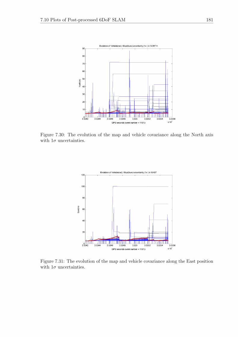
7.10 Plots of Post-processed 6DoF SLAM 181
Figure 7.30: The evolution of the map and vehicle covariance along the North axiswith 1σ uncertainties.
Figure 7.31: The evolution of the map and vehicle covariance along the East positionwith 1σ uncertainties.
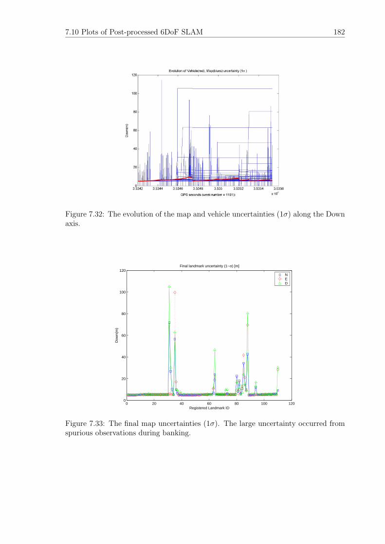
7.10 Plots of Post-processed 6DoF SLAM 182
Figure 7.32: The evolution of the map and vehicle uncertainties (1σ) along the Downaxis.
0 20 40 60 80 100 1200
20
40
60
80
100
120Final landmark uncertainty (1−σ) [m]
Dow
n(m
)
Registered Landmark ID
NED
Figure 7.33: The final map uncertainties (1σ). The large uncertainty occurred fromspurious observations during banking.
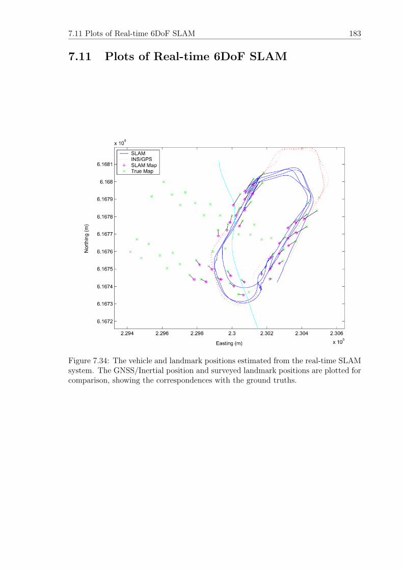
7.11 Plots of Real-time 6DoF SLAM 183
7.11 Plots of Real-time 6DoF SLAM
Figure 7.34: The vehicle and landmark positions estimated from the real-time SLAMsystem. The GNSS/Inertial position and surveyed landmark positions are plotted forcomparison, showing the correspondences with the ground truths.
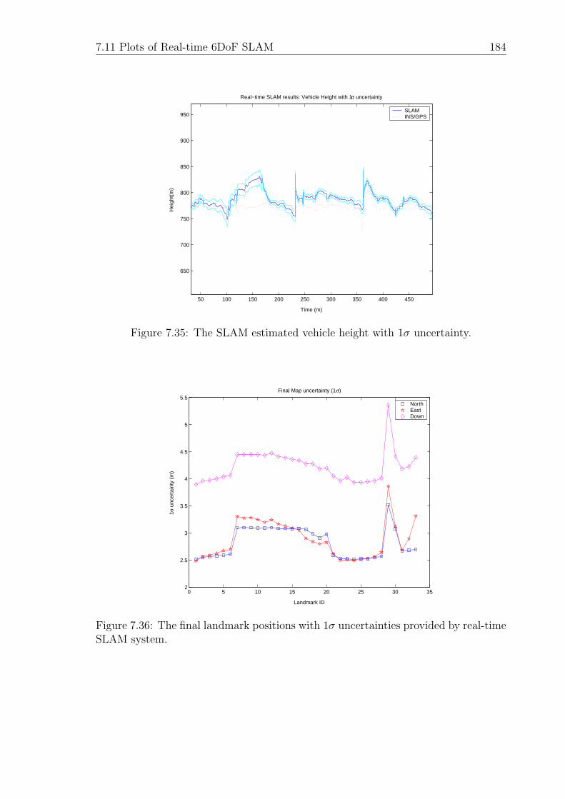
7.11 Plots of Real-time 6DoF SLAM 184
50 100 150 200 250 300 350 400 450
650
700
750
800
850
900
950
Real−time SLAM results: Vehicle Height with 1σ uncertainty
Time (m)
Hei
ght(
m)
SLAMINS/GPS
Figure 7.35: The SLAM estimated vehicle height with 1σ uncertainty.
0 5 10 15 20 25 30 352
2.5
3
3.5
4
4.5
5
5.5Final Map uncertainty (1σ)
Landmark ID
1σ u
ncer
tain
ty (
m)
NorthEastDown
Figure 7.36: The final landmark positions with 1σ uncertainties provided by real-timeSLAM system.
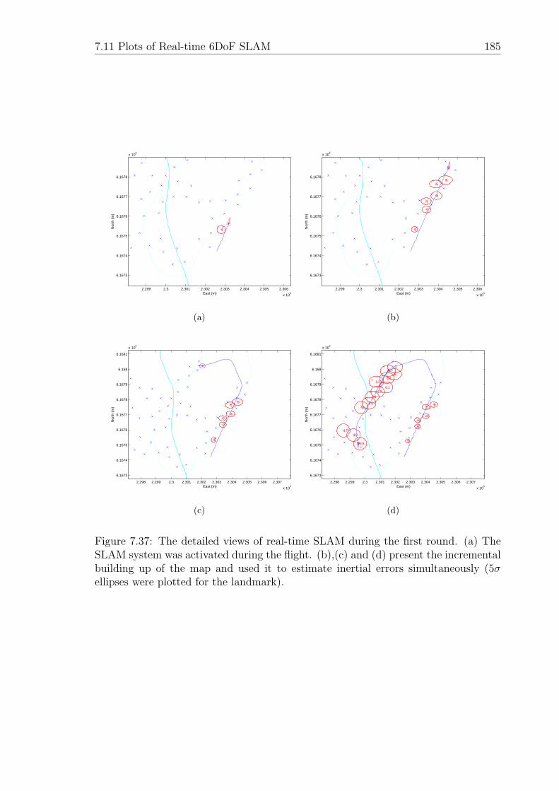
7.11 Plots of Real-time 6DoF SLAM 185
2.299 2.3 2.301 2.302 2.303 2.304 2.305 2.306
x 105
6.1673
6.1674
6.1675
6.1676
6.1677
6.1678
x 106
East (m)
Nor
th (
m)
1
(a)
2.299 2.3 2.301 2.302 2.303 2.304 2.305 2.306
x 105
6.1673
6.1674
6.1675
6.1676
6.1677
6.1678
x 106
East (m)
Nor
th (
m)
1
2
3
4
56
(b)
2.298 2.299 2.3 2.301 2.302 2.303 2.304 2.305 2.306 2.307
x 105
6.1673
6.1674
6.1675
6.1676
6.1677
6.1678
6.1679
6.168
6.1681
x 106
East (m)
Nor
th (
m)
1
2
34
56
(c)
2.298 2.299 2.3 2.301 2.302 2.303 2.304 2.305 2.306 2.307
x 105
6.1673
6.1674
6.1675
6.1676
6.1677
6.1678
6.1679
6.168
6.1681
x 106
East (m)
Nor
th (
m)
1
2
34
56
7
89
10
11
12
1314
1516
1718
19
(d)
Figure 7.37: The detailed views of real-time SLAM during the first round. (a) TheSLAM system was activated during the flight. (b),(c) and (d) present the incrementalbuilding up of the map and used it to estimate inertial errors simultaneously (5σellipses were plotted for the landmark).
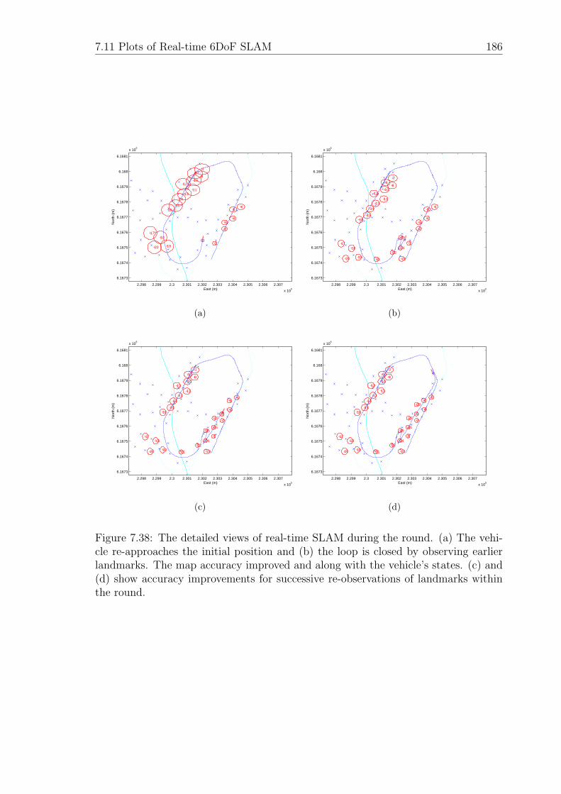
7.11 Plots of Real-time 6DoF SLAM 186
2.298 2.299 2.3 2.301 2.302 2.303 2.304 2.305 2.306 2.307
x 105
6.1673
6.1674
6.1675
6.1676
6.1677
6.1678
6.1679
6.168
6.1681
x 106
East (m)
Nor
th (
m)
1
2
34
56
7
89
10
11
12
1314
1516
1718
1920
(a)
2.298 2.299 2.3 2.301 2.302 2.303 2.304 2.305 2.306 2.307
x 105
6.1673
6.1674
6.1675
6.1676
6.1677
6.1678
6.1679
6.168
6.1681
x 106
East (m)
Nor
th (
m)
1
2
34
56
7
89
10
11
12
13
14
1516
1718
1920 21
22
23
24
25
(b)
2.298 2.299 2.3 2.301 2.302 2.303 2.304 2.305 2.306 2.307
x 105
6.1673
6.1674
6.1675
6.1676
6.1677
6.1678
6.1679
6.168
6.1681
x 106
East (m)
Nor
th (
m)
1
2
34
56
7
89
10
11
12
13
14
1516
1718
1920 21
22
23
24
2526
27
(c)
2.298 2.299 2.3 2.301 2.302 2.303 2.304 2.305 2.306 2.307
x 105
6.1673
6.1674
6.1675
6.1676
6.1677
6.1678
6.1679
6.168
6.1681
x 106
East (m)
Nor
th (
m)
1
2
34
56
7
89
10
11
12
13
14
1516
1718
1920 21
22
23
24
2526
27
28
(d)
Figure 7.38: The detailed views of real-time SLAM during the round. (a) The vehi-cle re-approaches the initial position and (b) the loop is closed by observing earlierlandmarks. The map accuracy improved and along with the vehicle’s states. (c) and(d) show accuracy improvements for successive re-observations of landmarks withinthe round.
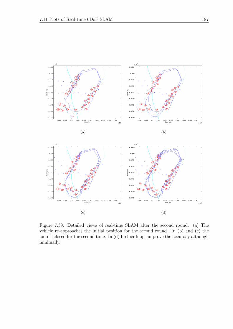
7.11 Plots of Real-time 6DoF SLAM 187
2.298 2.299 2.3 2.301 2.302 2.303 2.304 2.305 2.306 2.307
x 105
6.1673
6.1674
6.1675
6.1676
6.1677
6.1678
6.1679
6.168
6.1681
x 106
East (m)
Nor
th (
m)
1
2
34
56
7
89
10
1112
13
14
1516
1718
1920 21
22
23
24
2526
27
28
29
(a)
2.298 2.299 2.3 2.301 2.302 2.303 2.304 2.305 2.306 2.307
x 105
6.1673
6.1674
6.1675
6.1676
6.1677
6.1678
6.1679
6.168
6.1681
x 106
East (m)
Nor
th (
m)
1
2
34
56
7
89
10
1112
13
14
1516
1718
1920 21
2223
24
2526
27
28
29
(b)
2.298 2.299 2.3 2.301 2.302 2.303 2.304 2.305 2.306 2.307
x 105
6.1673
6.1674
6.1675
6.1676
6.1677
6.1678
6.1679
6.168
6.1681
x 106
East (m)
Nor
th (
m)
1
2
34
56
7
89
10
1112
13
14
1516
1718
1920 21
2223
24
2526
27
28
29
30
31
32
33
(c)
2.298 2.299 2.3 2.301 2.302 2.303 2.304 2.305 2.306 2.307
x 105
6.1673
6.1674
6.1675
6.1676
6.1677
6.1678
6.1679
6.168
6.1681
x 106
East (m)
Nor
th (
m)
1
2
34
56
7
89
10
1112
13
14
1516
1718
1920 21
2223
24
2526
27
28
29
30
31
32
33
(d)
Figure 7.39: Detailed views of real-time SLAM after the second round. (a) Thevehicle re-approaches the initial position for the second round. In (b) and (c) theloop is closed for the second time. In (d) further loops improve the accuracy althoughminimally.
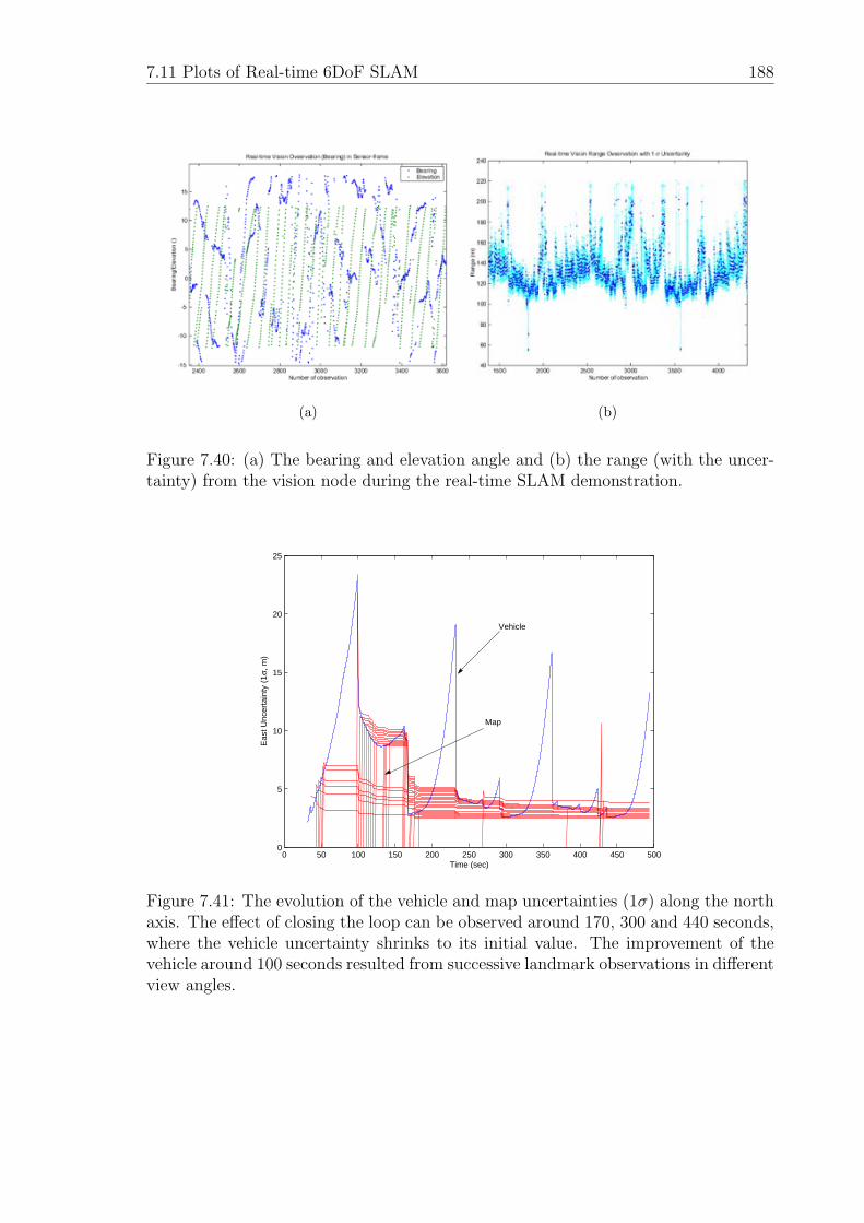
7.11 Plots of Real-time 6DoF SLAM 188
(a) (b)
Figure 7.40: (a) The bearing and elevation angle and (b) the range (with the uncer-tainty) from the vision node during the real-time SLAM demonstration.
0 50 100 150 200 250 300 350 400 450 5000
5
10
15
20
25
Time (sec)
Eas
t Unc
erta
inty
(1
σ, m
)
Vehicle
Map
Figure 7.41: The evolution of the vehicle and map uncertainties (1σ) along the northaxis. The effect of closing the loop can be observed around 170, 300 and 440 seconds,where the vehicle uncertainty shrinks to its initial value. The improvement of thevehicle around 100 seconds resulted from successive landmark observations in differentview angles.
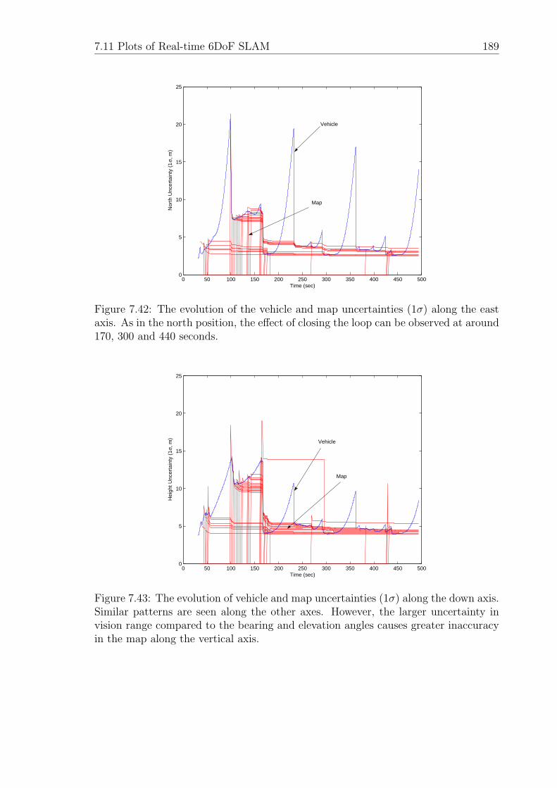
7.11 Plots of Real-time 6DoF SLAM 189
0 50 100 150 200 250 300 350 400 450 5000
5
10
15
20
25
Time (sec)
Nor
th U
ncer
tain
ty (
1σ,
m)
Vehicle
Map
Figure 7.42: The evolution of the vehicle and map uncertainties (1σ) along the eastaxis. As in the north position, the effect of closing the loop can be observed at around170, 300 and 440 seconds.
0 50 100 150 200 250 300 350 400 450 5000
5
10
15
20
25
Time (sec)
Hei
ght U
ncer
tain
ty (
1σ,
m)
Vehicle
Map
Figure 7.43: The evolution of vehicle and map uncertainties (1σ) along the down axis.Similar patterns are seen along the other axes. However, the larger uncertainty invision range compared to the bearing and elevation angles causes greater inaccuracyin the map along the vertical axis.
Chapter 8
Further Analysis on AirborneSLAM
8.1 Introduction
The previous chapter presented results on airborne SLAM which illustrated its use-
fulness as an autonomous navigation system. This chapter provides further analysis
to verify and assess the 6DoF SLAM algorithms under various scenarios and different
filter configurations.
Firstly, an analysis of the effect on SLAM performance will be provided given
different environment sensors, in particular focusing on a vision and radar sensor
with different field-of-views (or coverage) and observation accuracies.
Secondly, the indirect SLAM algorithm which was developed in Chapter 4 will be
compared to the nonlinear direct implementation. The main benefit of this approach
is the computational savings encountered in the prediction cycle, and hence results
are presented with various prediction rates.
Thirdly, the DDF 6DoF SLAM results will be provide two platforms platforms
undertaking SLAM which also share map information with one another. The result
of full map communication is compared to the case when no maps are communicated.
8.2 Analysis of Varying Sensor Characteristics on SLAM 191
Finally, since the process model in indirect SLAM is of a linear time-variant na-
ture, questions can now be asked about the observability of SLAM. The observability
analysis will be conducted and some interesting results presented.
In this chapter the analysis of SLAM will be presented using the Hardware in
the Loop system presented in the previous chapter which was used to validate the
algorithms before flight demonstrations.
8.2 Analysis of Varying Sensor Characteristics on
SLAM
This section looks at how varying the characteristics of the mission sensor affects
SLAM performance in localisation and mapping. Two kinds of on-board sensors are
simulated: a vision sensor (CASE I) and a radar sensor (CASE II).
CASE I simulates the vision sensor used in the real system with predicted range
based on knowledge of target size. CASE II simulates a proposed radar sensor which
is to be developed for the project. Figure 8.1 compares the FOV between these two
sensors.
The vision observation is expressed in a camera frame which requires coordinate
transformation to be processed in the SLAM node. However, the observation from
the radar sensor is expressed in its gimbal frame where the X and Y axes coincide
with the local-level frame and the Z axis coincides with yaw axis of the vehicle. Hence
the sensor to body transformation matrix differs in each sensor.
The simulation parameters are listed in Table 8.1. The table also includes a
vision/laser sensor which is also to be developed for the project in order to improve
range accuracy, and this will be presented in the following section for the analysis on
indirect SLAM. The flight trajectory is a “figure of eight” with an altitude of 100m.
The flight time is 300 seconds and the average flight speed is 40m/s.
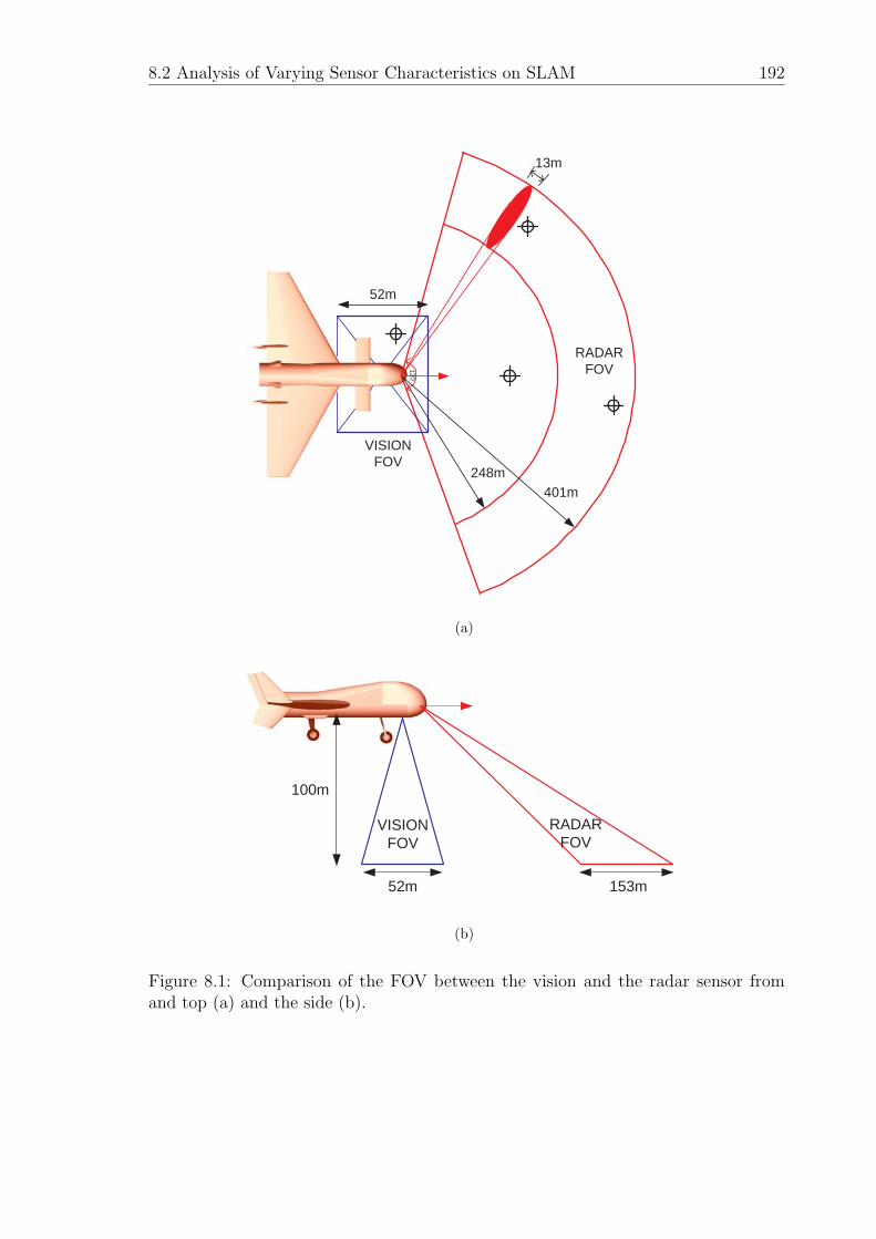
8.2 Analysis of Varying Sensor Characteristics on SLAM 192
13m
120
52m
401m248m
RADARFOV
VISIONFOV
(a)
100m
52m 153m
RADARFOV
VISIONFOV
(b)
Figure 8.1: Comparison of the FOV between the vision and the radar sensor fromand top (a) and the side (b).
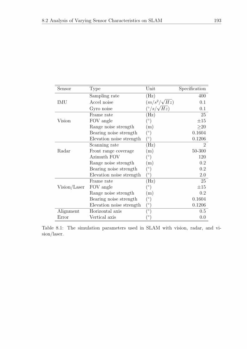
8.2 Analysis of Varying Sensor Characteristics on SLAM 193
Sensor Type Unit Specification
Sampling rate (Hz) 400
IMU Accel noise (m/s2/√Hz) 0.1
Gyro noise (◦/s/√Hz) 0.1
Frame rate (Hz) 25Vision FOV angle (◦) ±15
Range noise strength (m) ≥20Bearing noise strength (◦) 0.1604Elevation noise strength (◦) 0.1206Scanning rate (Hz) 2
Radar Front range coverage (m) 50-300Azimuth FOV (◦) 120Range noise strength (m) 0.2Bearing noise strength (◦) 0.2Elevation noise strength (◦) 2.0Frame rate (Hz) 25
Vision/Laser FOV angle (◦) ±15Range noise strength (m) 0.2Bearing noise strength (◦) 0.1604Elevation noise strength (◦) 0.1206
Alignment Horizontal axis (◦) 0.5Error Vertical axis (◦) 0.0
Table 8.1: The simulation parameters used in SLAM with vision, radar, and vi-sion/laser.
8.2 Analysis of Varying Sensor Characteristics on SLAM 194
8.2.1 A Comparison Between the Vision and Radar Sensors
The results using a vision sensor are plotted in Figures 8.3 to 8.9. The vision sensor
detects the landmark below the vehicle and registers 19 landmarks from the total of
50 landmarks on the ground. The landmark extraction rate is 25Hz, but due to the
limited FOV and sparse placement of the landmarks, the vehicle covariance increases
and results in a 20m correction at the end of the first round as shown in Figure 8.4.
It can be seen from Figure 8.7 that the initial alignment error on the roll and pitch
axes are observable and corrected within one round while the heading begins to be
corrected after the first round. Figure 8.8 depicts the map covariance changes during
flight. In the first two rounds, the map has large uncertainty because it is initialised
from the vehicle which also has large uncertainty. After the second loop, the map
improves and constrains the drift rates of the vehicle whenever an observation occurs.
The final map accuracy achieved was under 5.8m where the initial vehicle uncertainty
was 5m.
The SLAM results using a radar sensor are presented from Figure 8.10 to 8.18. The
radar has 50-300m range coverage and 120◦ foreground scanning coverage. Figure 8.10
shows that the vehicle registered all of the landmarks during flight with accuracies as
shown in Figure 8.18. Figures 8.11 to 8.13 shows that better estimates of the vehicle
states occurs. Figures 8.15 to 8.17 present the map covariance changes where trends
are similar to Case I but show better accuracy.
The analysis between CASE I and CASE II is summarised in Table 8.2. From
this result, it can be seen that the vehicle accuracy is greatly affected by the FOV
of the environment sensor. The wider FOV guarantees longer observation time for
landmarks which in turn provides a better capability of constraining the INS error.
In contrast the limited FOV in Case I introduced larger a horizontal drift until the
vehicle closed the loop.
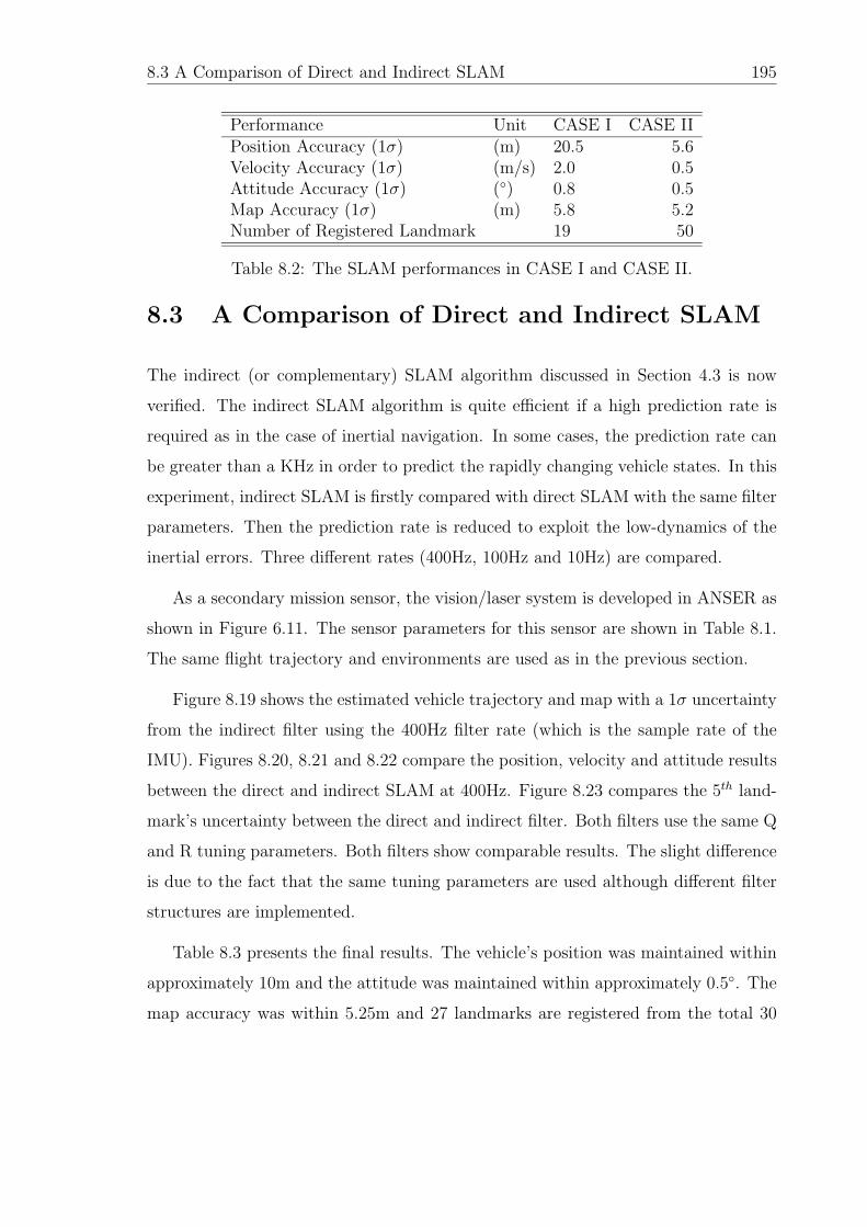
8.3 A Comparison of Direct and Indirect SLAM 195
Performance Unit CASE I CASE IIPosition Accuracy (1σ) (m) 20.5 5.6Velocity Accuracy (1σ) (m/s) 2.0 0.5Attitude Accuracy (1σ) (◦) 0.8 0.5Map Accuracy (1σ) (m) 5.8 5.2Number of Registered Landmark 19 50
Table 8.2: The SLAM performances in CASE I and CASE II.
8.3 A Comparison of Direct and Indirect SLAM
The indirect (or complementary) SLAM algorithm discussed in Section 4.3 is now
verified. The indirect SLAM algorithm is quite efficient if a high prediction rate is
required as in the case of inertial navigation. In some cases, the prediction rate can
be greater than a KHz in order to predict the rapidly changing vehicle states. In this
experiment, indirect SLAM is firstly compared with direct SLAM with the same filter
parameters. Then the prediction rate is reduced to exploit the low-dynamics of the
inertial errors. Three different rates (400Hz, 100Hz and 10Hz) are compared.
As a secondary mission sensor, the vision/laser system is developed in ANSER as
shown in Figure 6.11. The sensor parameters for this sensor are shown in Table 8.1.
The same flight trajectory and environments are used as in the previous section.
Figure 8.19 shows the estimated vehicle trajectory and map with a 1σ uncertainty
from the indirect filter using the 400Hz filter rate (which is the sample rate of the
IMU). Figures 8.20, 8.21 and 8.22 compare the position, velocity and attitude results
between the direct and indirect SLAM at 400Hz. Figure 8.23 compares the 5th land-
mark’s uncertainty between the direct and indirect filter. Both filters use the same Q
and R tuning parameters. Both filters show comparable results. The slight difference
is due to the fact that the same tuning parameters are used although different filter
structures are implemented.
Table 8.3 presents the final results. The vehicle’s position was maintained within
approximately 10m and the attitude was maintained within approximately 0.5◦. The
map accuracy was within 5.25m and 27 landmarks are registered from the total 30
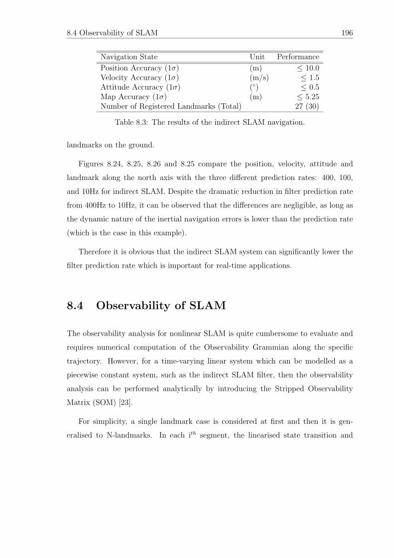
8.4 Observability of SLAM 196
Navigation State Unit Performance
Position Accuracy (1σ) (m) ≤ 10.0Velocity Accuracy (1σ) (m/s) ≤ 1.5Attitude Accuracy (1σ) (◦) ≤ 0.5Map Accuracy (1σ) (m) ≤ 5.25Number of Registered Landmarks (Total) 27 (30)
Table 8.3: The results of the indirect SLAM navigation.
landmarks on the ground.
Figures 8.24, 8.25, 8.26 and 8.25 compare the position, velocity, attitude and
landmark along the north axis with the three different prediction rates: 400, 100,
and 10Hz for indirect SLAM. Despite the dramatic reduction in filter prediction rate
from 400Hz to 10Hz, it can be observed that the differences are negligible, as long as
the dynamic nature of the inertial navigation errors is lower than the prediction rate
(which is the case in this example).
Therefore it is obvious that the indirect SLAM system can significantly lower the
filter prediction rate which is important for real-time applications.
8.4 Observability of SLAM
The observability analysis for nonlinear SLAM is quite cumbersome to evaluate and
requires numerical computation of the Observability Grammian along the specific
trajectory. However, for a time-varying linear system which can be modelled as a
piecewise constant system, such as the indirect SLAM filter, then the observability
analysis can be performed analytically by introducing the Stripped Observability
Matrix (SOM) [23].
For simplicity, a single landmark case is considered at first and then it is gen-
eralised to N-landmarks. In each ith segment, the linearised state transition and
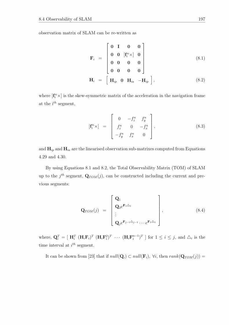
8.4 Observability of SLAM 197
observation matrix of SLAM can be re-written as
Fi =
⎡⎢⎢⎢⎢⎢⎣
0 I 0 0
0 0 [fni ×] 0
0 0 0 0
0 0 0 0
⎤⎥⎥⎥⎥⎥⎦ (8.1)
Hi =[
Hip 0 Hia −Hip
], (8.2)
where [fni ×] is the skew-symmetric matrix of the acceleration in the navigation frame
at the ith segment,
[fni ×] =
⎡⎢⎢⎢⎣
0 −fnz fny
fnz 0 −fnx−fny fnx 0
⎤⎥⎥⎥⎦ , (8.3)
and Hip and Hia are the linearised observation sub-matrixes computed from Equations
4.29 and 4.30.
By using Equations 8.1 and 8.2, the Total Observability Matrix (TOM) of SLAM
up to the jth segment, QTOM(j), can be constructed including the current and pre-
vious segments:
QTOM(j) =
⎡⎢⎢⎢⎢⎢⎣
Q1
Q2eF1�1
...
QjeFj−1�j−1 · · · eF1�1
⎤⎥⎥⎥⎥⎥⎦ , (8.4)
where, QTi = [ HT
i (HiFi)T (HiF
2i )T · · · (HiF
n−1i )T ] for 1 ≤ i ≤ j, and �i is the
time interval at ith segment.
It can be shown from [23] that if null(Qi) ⊂ null(Fi), ∀i, then rank(QTOM(j)) =
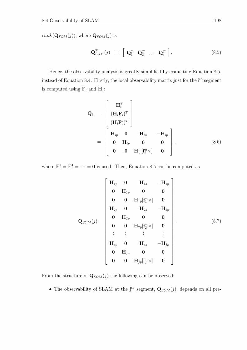
8.4 Observability of SLAM 198
rank(QSOM(j)), where QSOM(j) is
QTSOM(j) =
[QT
1 QT2 . . . QT
j
]. (8.5)
Hence, the observability analysis is greatly simplified by evaluating Equation 8.5,
instead of Equation 8.4. Firstly, the local observability matrix just for the ith segment
is computed using Fi and Hi:
Qi =
⎡⎢⎢⎢⎣
HTi
(HiFi)T
(HiF2i )T
⎤⎥⎥⎥⎦
=
⎡⎢⎢⎢⎣
Hip 0 Hia −Hip
0 Hip 0 0
0 0 Hip[fni ×] 0
⎤⎥⎥⎥⎦ , (8.6)
where F3i = F4
i = · · · = 0 is used. Then, Equation 8.5 can be computed as
QSOM(j) =
⎡⎢⎢⎢⎢⎢⎢⎢⎢⎢⎢⎢⎢⎢⎢⎢⎢⎢⎢⎢⎢⎢⎢⎢⎣
H1p 0 H1a −H1p
0 H1p 0 0
0 0 H1p[fn1 ×] 0
H2p 0 H2a −H2p
0 H2p 0 0
0 0 H2p[fn2 ×] 0
......
......
Hjp 0 Hja −Hjp
0 Hjp 0 0
0 0 Hjp[fnj ×] 0
⎤⎥⎥⎥⎥⎥⎥⎥⎥⎥⎥⎥⎥⎥⎥⎥⎥⎥⎥⎥⎥⎥⎥⎥⎦
. (8.7)
From the structure of QSOM(j) the following can be observed:
• The observability of SLAM at the jth segment, QSOM(j), depends on all pre-
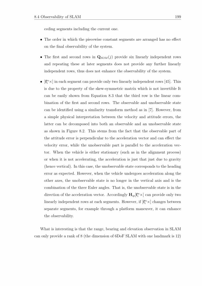
8.4 Observability of SLAM 199
ceding segments including the current one.
• The order in which the piecewise constant segments are arranged has no effect
on the final observability of the system.
• The first and second rows in QSOM(j) provide six linearly independent rows
and repeating these at later segments does not provide any further linearly
independent rows, thus does not enhance the observability of the system.
• [fni ×] in each segment can provide only two linearly independent rows [45]. This
is due to the property of the skew-symmetric matrix which is not invertible It
can be easily shown from Equation 8.3 that the third row is the linear com-
bination of the first and second rows. The observable and unobservable state
can be identified using a similarity transform method as in [7]. However, from
a simple physical interpretation between the velocity and attitude errors, the
latter can be decomposed into both an observable and an unobservable state
as shown in Figure 8.2. This stems from the fact that the observable part of
the attitude error is perpendicular to the acceleration vector and can effect the
velocity error, while the unobservable part is parallel to the acceleration vec-
tor. When the vehicle is either stationary (such as in the alignment process)
or when it is not accelerating, the acceleration is just that just due to gravity
(hence vertical). In this case, the unobservable state corresponds to the heading
error as expected. However, when the vehicle undergoes acceleration along the
other axes, the unobservable state is no longer in the vertical axis and is the
combination of the three Euler angles. That is, the unobservable state is in the
direction of the acceleration vector. Accordingly Hip[fni ×] can provide only two
linearly independent rows at each segments. However, if [fni ×] changes between
separate segments, for example through a platform maneuver, it can enhance
the observability.
What is interesting is that the range, bearing and elevation observation in SLAM
can only provide a rank of 8 (the dimension of 6DoF SLAM with one landmark is 12)
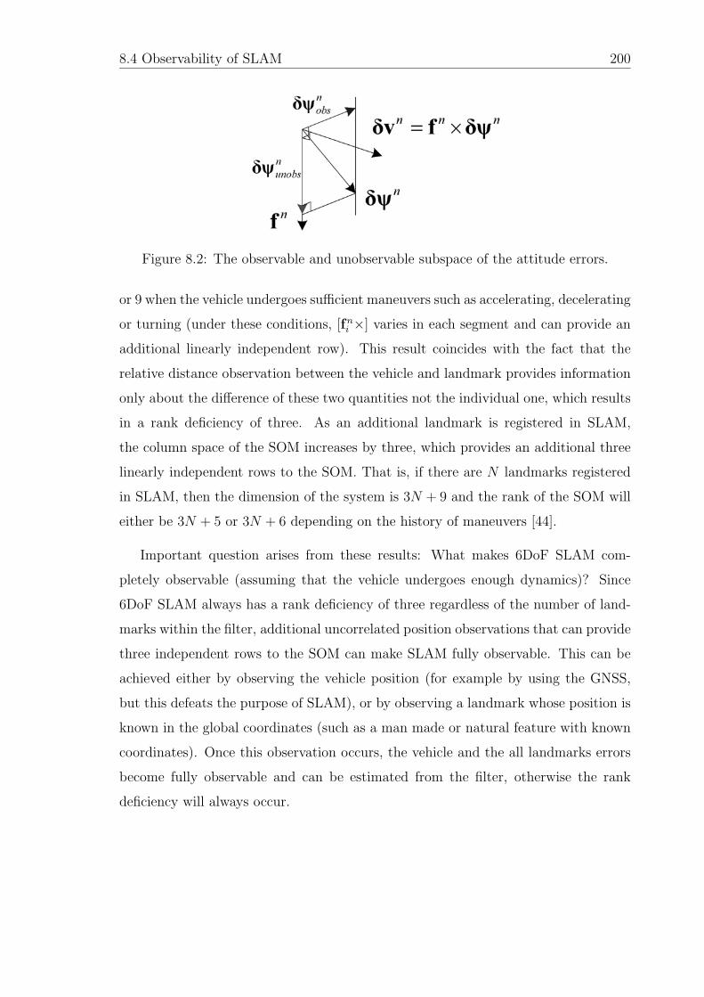
8.4 Observability of SLAM 200
Figure 8.2: The observable and unobservable subspace of the attitude errors.
or 9 when the vehicle undergoes sufficient maneuvers such as accelerating, decelerating
or turning (under these conditions, [fni ×] varies in each segment and can provide an
additional linearly independent row). This result coincides with the fact that the
relative distance observation between the vehicle and landmark provides information
only about the difference of these two quantities not the individual one, which results
in a rank deficiency of three. As an additional landmark is registered in SLAM,
the column space of the SOM increases by three, which provides an additional three
linearly independent rows to the SOM. That is, if there are N landmarks registered
in SLAM, then the dimension of the system is 3N + 9 and the rank of the SOM will
either be 3N + 5 or 3N + 6 depending on the history of maneuvers [44].
Important question arises from these results: What makes 6DoF SLAM com-
pletely observable (assuming that the vehicle undergoes enough dynamics)? Since
6DoF SLAM always has a rank deficiency of three regardless of the number of land-
marks within the filter, additional uncorrelated position observations that can provide
three independent rows to the SOM can make SLAM fully observable. This can be
achieved either by observing the vehicle position (for example by using the GNSS,
but this defeats the purpose of SLAM), or by observing a landmark whose position is
known in the global coordinates (such as a man made or natural feature with known
coordinates). Once this observation occurs, the vehicle and the all landmarks errors
become fully observable and can be estimated from the filter, otherwise the rank
deficiency will always occur.
8.5 DDF 6DoF SLAM 201
It should be noted that the rank deficiency of three in SLAM is not a problem
for the purpose of localisation and relative mapping. With sufficient re-observations,
the relative errors between the vehicle and landmark will converge to zero, while the
actual state errors will not due to their initial errors. In other words, if the relative
errors become zero, the filter will not generate corrections, which will result in perfect
localisation within the relative map. However, there will still exist uncertainties
in the vehicle state and map position which the rank deficiency is implying. Any
uncorrelated observation of the vehicle or landmark position will make their errors
observable.
If SLAM is fully observable, then the ability to estimate the state of SLAM is only
dependent on 1) the statistical characteristics of the noise both in the process and
observation model and 2) the relative geometry between the vehicle and landmarks.
The former factor can be analysed through the probability density distribution of the
noise. The latter one is related to the sensitivity of the observation matrix and can
be studied by analysing the information contributions from the spatially distributed
information sources (this issue is not tackled in this paper. However the concept was
applied to the optimal configuration of the skewed redundant inertial sensors and can
be seen in [71]).
8.5 DDF 6DoF SLAM
This section presents results for the DDF SLAM algorithm for a 6DoF platform which
uses the information filter.
The same simulation parameters which are shown in Table 8.1 are used to demon-
strate airborne DDF SLAM using the INS and vision sensor. In the simulation, two
flight vehicles undergo part of a figure-of-eight trajectory approximately 100m above
the ground with average flight speeds of 40m/s. In each DDF local filter, the vehicle
model is updated every 400Hz, the vision landmark extraction rate is 25Hz and the
observation model is updated at 25Hz. The DDF SLAM update is performed every
8.5 DDF 6DoF SLAM 202
2 seconds. DDF SLAM with map communication is compared to SLAM without any
information communicated.
Figure 8.28 illustrates the 6DoF DDF SLAM result of UAV-1 with the estimated
vehicle and landmark position (5σ ellipsoids were used for clarification) and the final
landmark uncertainty. Since UAV-2 flies the other part of the figure-of-eight and is in
communication with UAV-1, the resulting map includes landmarks which this UAV
has not seen. The large uncertainty in landmark 3 was due to the high bank angle
during observation. Figure 8.29 shows the DDF SLAM result of UAV-2 with the
estimated vehicle and landmark position and the final landmark uncertainty.
Figures 8.30 and 8.31 present the standalone SLAM results without map commu-
nication. Both vehicles built maps with less landmarks and with larger uncertainty
than the DDF map. Landmark 9 in Figure 8.30(b) and landmark 1 in Figure 8.31(b)
correspond to the landmark-3 in the DDF map.
Figure 8.32 compares the vehicle position uncertainty with (dashed line) and with-
out (solid line) map communication. It can be observed that when map communi-
cation occurs, the accuracy of both vehicle positions improves immediately. Similar
results were obtained in velocity.
Figure 8.33 presents the heading angle result. As in the position result, both
vehicle headings are also improved. The rapid decrease of heading uncertainty in
UAV-1 at the beginning was due to the high maneuvers of UAV-1 at start time which
enhanced its heading observability, while UAV-2 undergoes relatively low maneuvers
at start time, resulting in a slower convergence rate.
From these results it is obvious that the DDF SLAM system can significantly
enhance the map and vehicle accuracy, since the communicated map information
improves the quality of the map and hence also indirectly the localisation accuracy
of the vehicle.
8.6 Summary 203
8.6 Summary
This chapter has provided further analysis airborne 6DoF SLAM. A vision and radar
sensor were simulated and compared. The results illustrated that both 6DoF SLAM
systems had the capability to estimate the INS drift and to build a map, while
the radar sensor showed better performance due to its wider field-of-view angle and
accuracy.
The indirect SLAM algorithm was then presented and compared to the direct
version. Three reduced filter prediction rates were applied to the indirect filter to
exploit the low frequency dynamics of the inertial errors. The results showed that
the performance of the indirect filter was comparable to the direct one, and it was
shown that the filter prediction rate can be reduced dramatically from 400Hz to 10Hz
without any significant degradation, which showed the efficiency of indirect SLAM.
An observability analysis of 6DoF SLAM was then performed. The results showed
that if there are N landmarks registered in SLAM, then the degree of observability
becomes either 3N + 5 or 3N + 6 (with 3N + 9 being full rank) depending on the
history of the maneuvers.
Finally, DDF 6DoF SLAM was then demonstrated. The complete map commu-
nication case was compared to the case without communication. It was shown that
through communication the enhancement of map accuracy indirectly improved the
vehicle’s position, velocity and attitude accuracy as well.
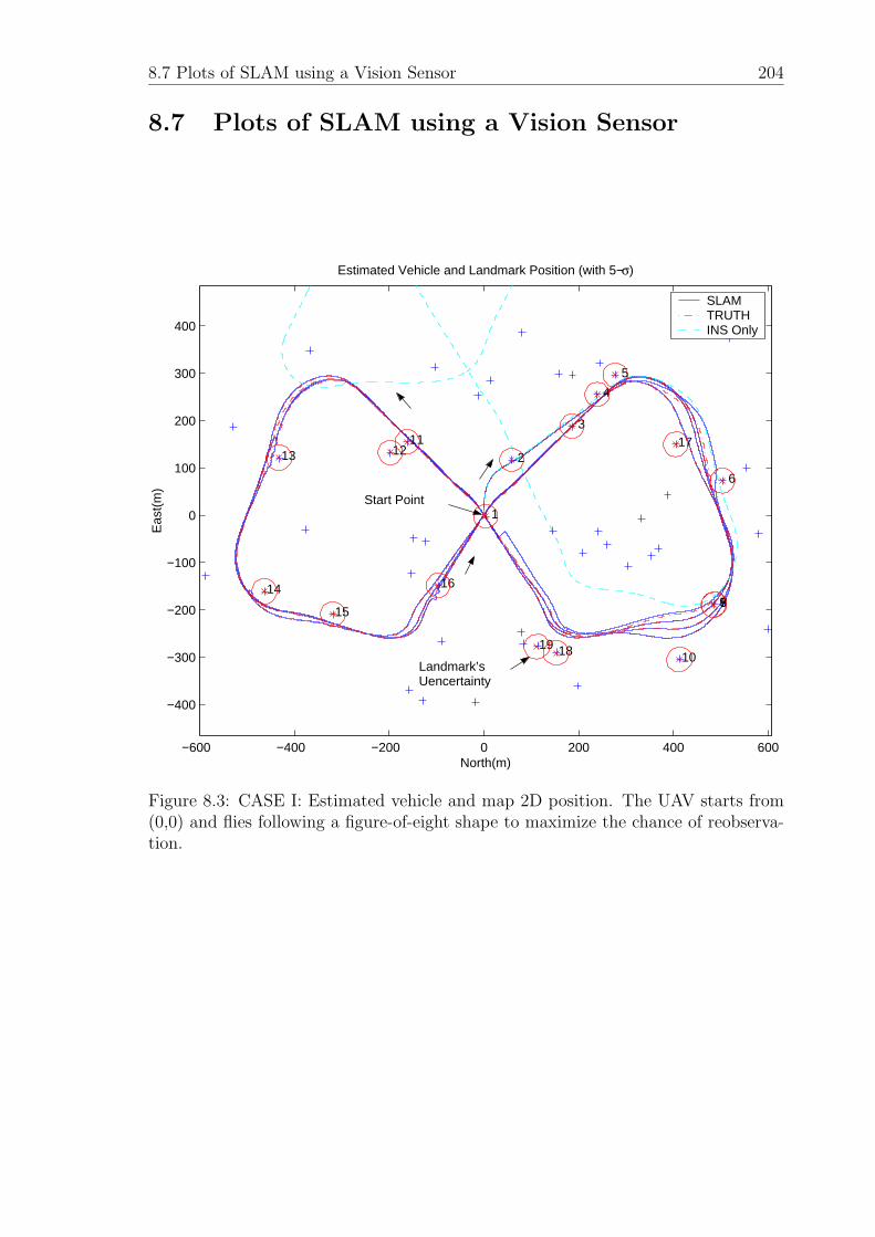
8.7 Plots of SLAM using a Vision Sensor 204
8.7 Plots of SLAM using a Vision Sensor
−600 −400 −200 0 200 400 600
−400
−300
−200
−100
0
100
200
300
400
Estimated Vehicle and Landmark Position (with 5−σ)
1
2
3
4
5
6
7 8 9
10
111213
14
15
16
17
1819
North(m)
Eas
t(m
)
SLAMTRUTHINS Only
Start Point
Landmark’s Uencertainty
Figure 8.3: CASE I: Estimated vehicle and map 2D position. The UAV starts from(0,0) and flies following a figure-of-eight shape to maximize the chance of reobserva-tion.
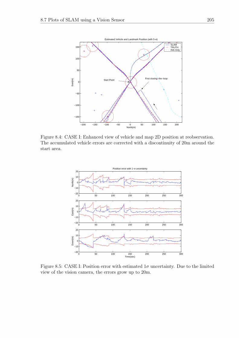
8.7 Plots of SLAM using a Vision Sensor 205
−200 −150 −100 −50 0 50 100 150 200
−150
−100
−50
0
50
100
150
Estimated Vehicle and Landmark Position (with 5−σ)
North(m)
Eas
t(m
)
SLAMTRUTHINS Only
First closing−the−loop Start Point
Figure 8.4: CASE I: Enhanced view of vehicle and map 2D position at reobservation.The accumulated vehicle errors are corrected with a discontinuity of 20m around thestart area.
0 50 100 150 200 250 300−20
−10
0
10
20Position error with 1−σ uncertainty
Nor
th(m
)
0 50 100 150 200 250 300−20
−10
0
10
20
Eas
t(m
)
0 50 100 150 200 250 300−20
−10
0
10
20
Dow
n(m
)
Time(sec)
Figure 8.5: CASE I: Position error with estimated 1σ uncertainty. Due to the limitedview of the vision camera, the errors grow up to 20m.
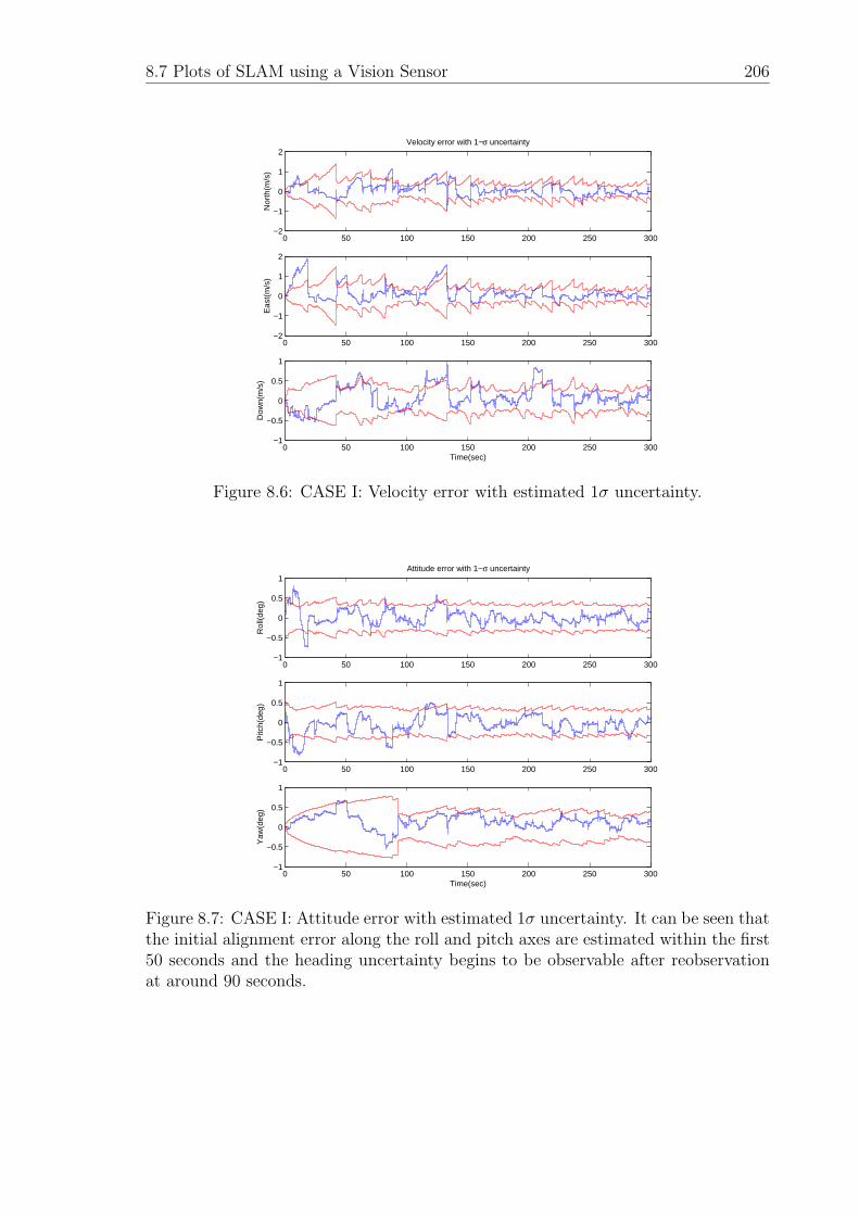
8.7 Plots of SLAM using a Vision Sensor 206
0 50 100 150 200 250 300−2
−1
0
1
2Velocity error with 1−σ uncertainty
Nor
th(m
/s)
0 50 100 150 200 250 300−2
−1
0
1
2E
ast(
m/s
)
0 50 100 150 200 250 300−1
−0.5
0
0.5
1
Dow
n(m
/s)
Time(sec)
Figure 8.6: CASE I: Velocity error with estimated 1σ uncertainty.
0 50 100 150 200 250 300−1
−0.5
0
0.5
1Attitude error with 1−σ uncertainty
Rol
l(deg
)
0 50 100 150 200 250 300−1
−0.5
0
0.5
1
Pitc
h(de
g)
0 50 100 150 200 250 300−1
−0.5
0
0.5
1
Yaw
(deg
)
Time(sec)
Figure 8.7: CASE I: Attitude error with estimated 1σ uncertainty. It can be seen thatthe initial alignment error along the roll and pitch axes are estimated within the first50 seconds and the heading uncertainty begins to be observable after reobservationat around 90 seconds.
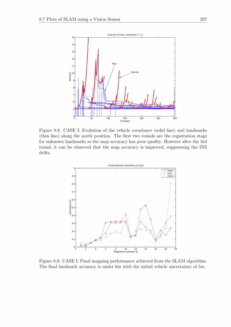
8.7 Plots of SLAM using a Vision Sensor 207
Figure 8.8: CASE I: Evolution of the vehicle covariance (solid line) and landmarks(thin line) along the north position. The first two rounds are the registration stagefor unknown landmarks so the map accuracy has poor quality. However after the 3rdround, it can be observed that the map accuracy is improved, suppressing the INSdrifts.
0 2 4 6 8 10 12 14 16 18 205
5.1
5.2
5.3
5.4
5.5
5.6
5.7
5.8
5.9
6Final landmark uncertainty (1σ) [m]
Unc
erta
inty
(m
)
Registered Landmark ID
NorthEastDown
Figure 8.9: CASE I: Final mapping performance achieved from the SLAM algorithm.The final landmark accuracy is under 6m with the initial vehicle uncertainty of 5m.
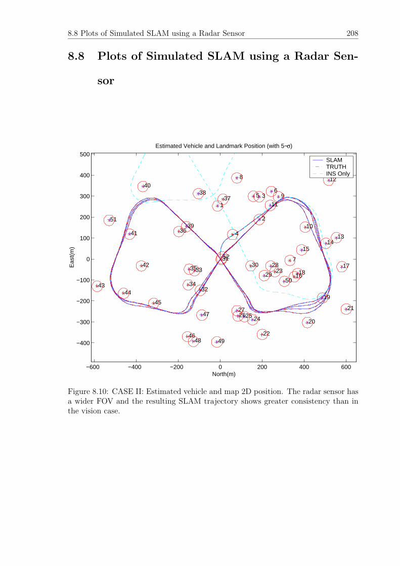
8.8 Plots of Simulated SLAM using a Radar Sensor 208
8.8 Plots of Simulated SLAM using a Radar Sen-
sor
−600 −400 −200 0 200 400 600
−400
−300
−200
−100
0
100
200
300
400
500Estimated Vehicle and Landmark Position (with 5−σ)
1
2
3
4
5 6
7
8
9
10
11
12
1314
15
16
1718
19
20
21
22
23
24252627
28
29
3031
32
33
34
35
36
3738
39
40
41
42
4344
45
46
47
48 49
50
51
52
North(m)
Eas
t(m
)
SLAMTRUTHINS Only
Figure 8.10: CASE II: Estimated vehicle and map 2D position. The radar sensor hasa wider FOV and the resulting SLAM trajectory shows greater consistency than inthe vision case.
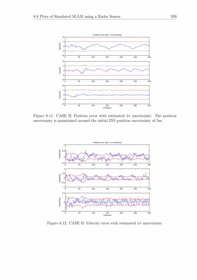
8.8 Plots of Simulated SLAM using a Radar Sensor 209
0 50 100 150 200 250 300−10
−5
0
5
10Position error with 1−σ uncertainty
Nor
th(m
)
0 50 100 150 200 250 300−10
−5
0
5
10E
ast(
m)
0 50 100 150 200 250 300−10
−5
0
5
10
Dow
n(m
)
Time(sec)
Figure 8.11: CASE II: Position error with estimated 1σ uncertainty. The positionuncertainty is maintained around the initial INS position uncertainty of 5m.
0 50 100 150 200 250 300−0.5
0
0.5
1Velocity error with 1−σ uncertainty
Nor
th(m
/s)
0 50 100 150 200 250 300−1
−0.5
0
0.5
1
Eas
t(m
/s)
0 50 100 150 200 250 300−0.5
0
0.5
Dow
n(m
/s)
Time(sec)
Figure 8.12: CASE II: Velocity error with estimated 1σ uncertainty.
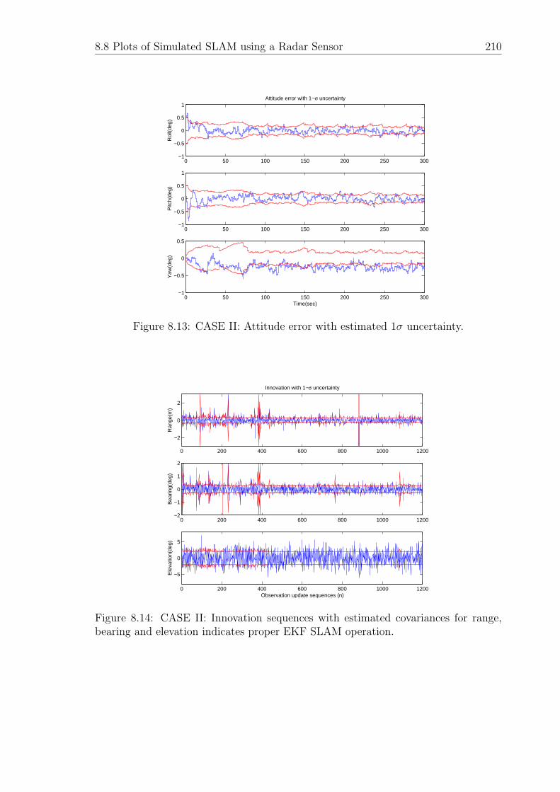
8.8 Plots of Simulated SLAM using a Radar Sensor 210
0 50 100 150 200 250 300−1
−0.5
0
0.5
1Attitude error with 1−σ uncertainty
Rol
l(deg
)
0 50 100 150 200 250 300−1
−0.5
0
0.5
1P
itch(
deg)
0 50 100 150 200 250 300−1
−0.5
0
0.5
Yaw
(deg
)
Time(sec)
Figure 8.13: CASE II: Attitude error with estimated 1σ uncertainty.
0 200 400 600 800 1000 1200
−2
0
2
Innovation with 1−σ uncertainty
Ran
ge(m
)
0 200 400 600 800 1000 1200−2
−1
0
1
2
Bea
ring(
deg)
0 200 400 600 800 1000 1200
−5
0
5
Ele
vatio
n(de
g)
Observation update sequences (n)
Figure 8.14: CASE II: Innovation sequences with estimated covariances for range,bearing and elevation indicates proper EKF SLAM operation.
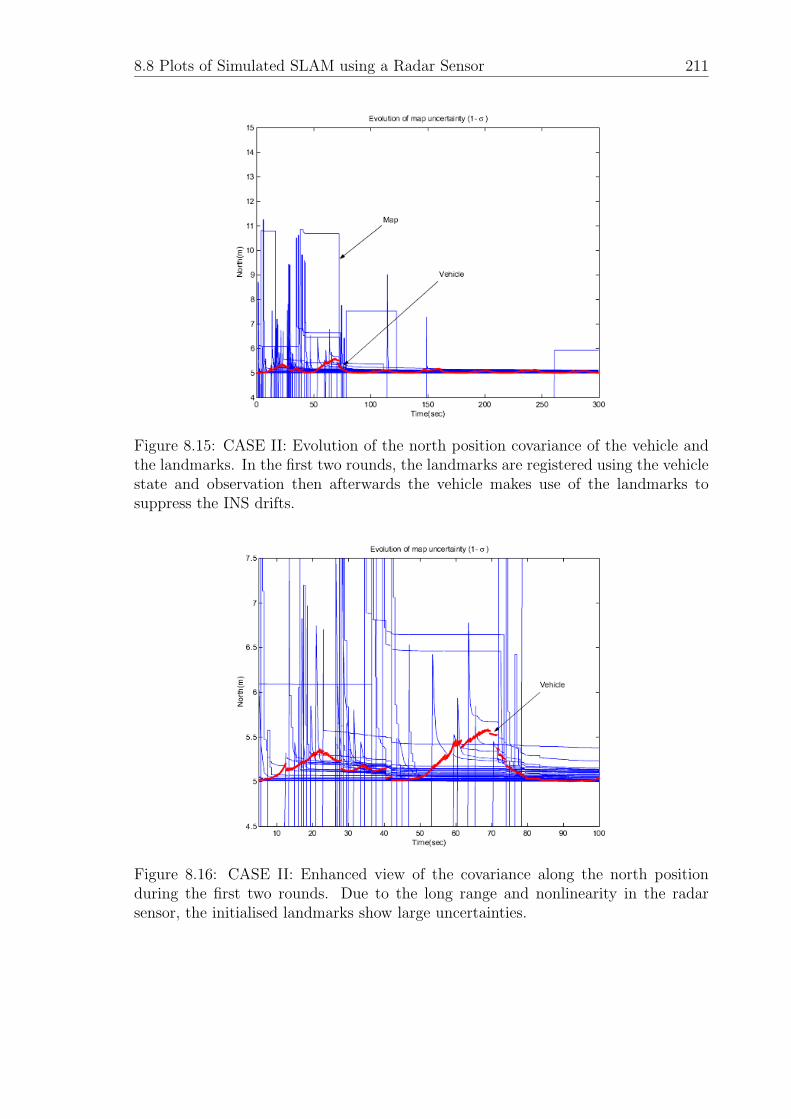
8.8 Plots of Simulated SLAM using a Radar Sensor 211
Figure 8.15: CASE II: Evolution of the north position covariance of the vehicle andthe landmarks. In the first two rounds, the landmarks are registered using the vehiclestate and observation then afterwards the vehicle makes use of the landmarks tosuppress the INS drifts.
Figure 8.16: CASE II: Enhanced view of the covariance along the north positionduring the first two rounds. Due to the long range and nonlinearity in the radarsensor, the initialised landmarks show large uncertainties.
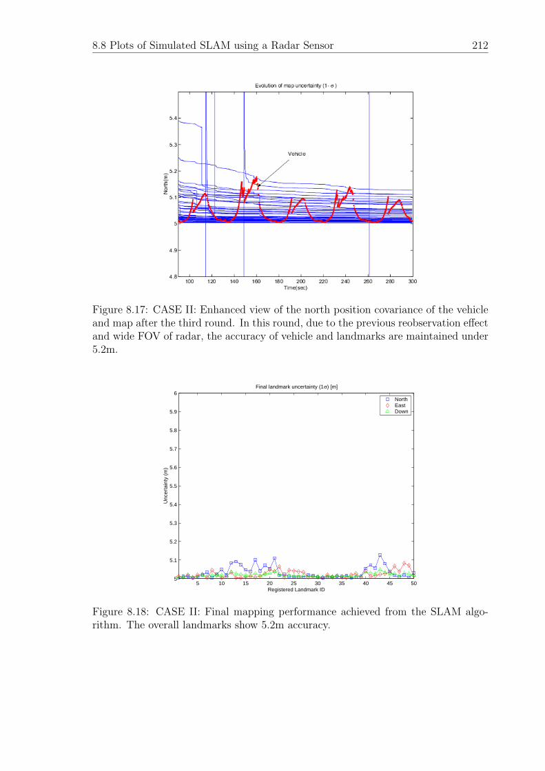
8.8 Plots of Simulated SLAM using a Radar Sensor 212
Figure 8.17: CASE II: Enhanced view of the north position covariance of the vehicleand map after the third round. In this round, due to the previous reobservation effectand wide FOV of radar, the accuracy of vehicle and landmarks are maintained under5.2m.
5 10 15 20 25 30 35 40 45 505
5.1
5.2
5.3
5.4
5.5
5.6
5.7
5.8
5.9
6Final landmark uncertainty (1σ) [m]
Unc
erta
inty
(m
)
Registered Landmark ID
NorthEastDown
Figure 8.18: CASE II: Final mapping performance achieved from the SLAM algo-rithm. The overall landmarks show 5.2m accuracy.
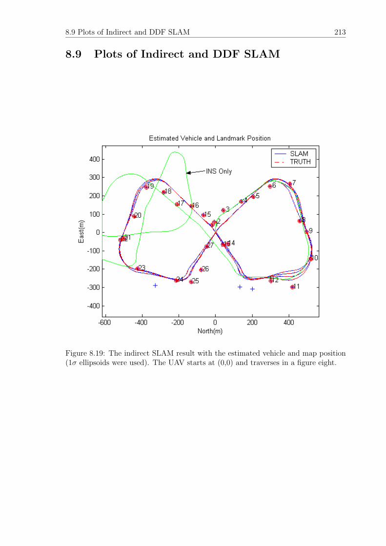
8.9 Plots of Indirect and DDF SLAM 213
8.9 Plots of Indirect and DDF SLAM
Figure 8.19: The indirect SLAM result with the estimated vehicle and map position(1σ ellipsoids were used). The UAV starts at (0,0) and traverses in a figure eight.
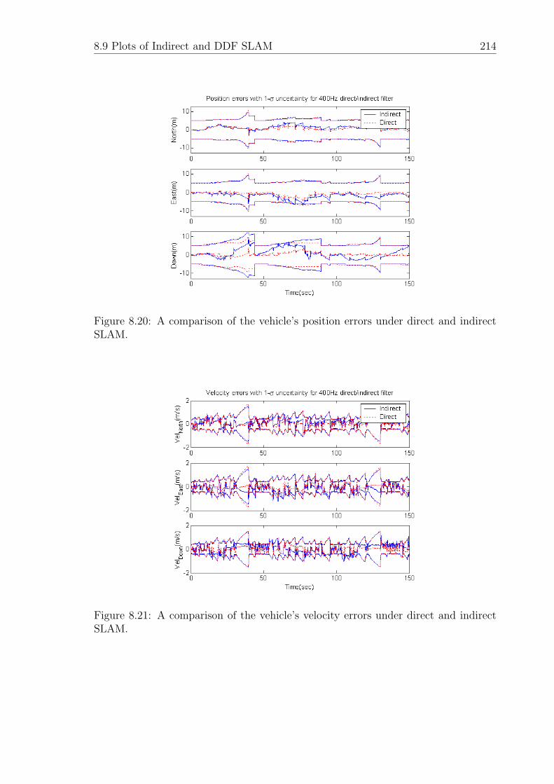
8.9 Plots of Indirect and DDF SLAM 214
Figure 8.20: A comparison of the vehicle’s position errors under direct and indirectSLAM.
Figure 8.21: A comparison of the vehicle’s velocity errors under direct and indirectSLAM.
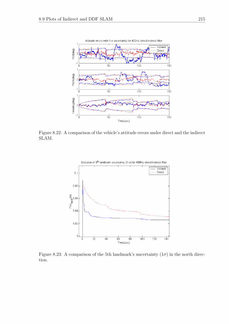
8.9 Plots of Indirect and DDF SLAM 215
Figure 8.22: A comparison of the vehicle’s attitude errors under direct and the indirectSLAM.
Figure 8.23: A comparison of the 5th landmark’s uncertainty (1σ) in the north direc-tion.
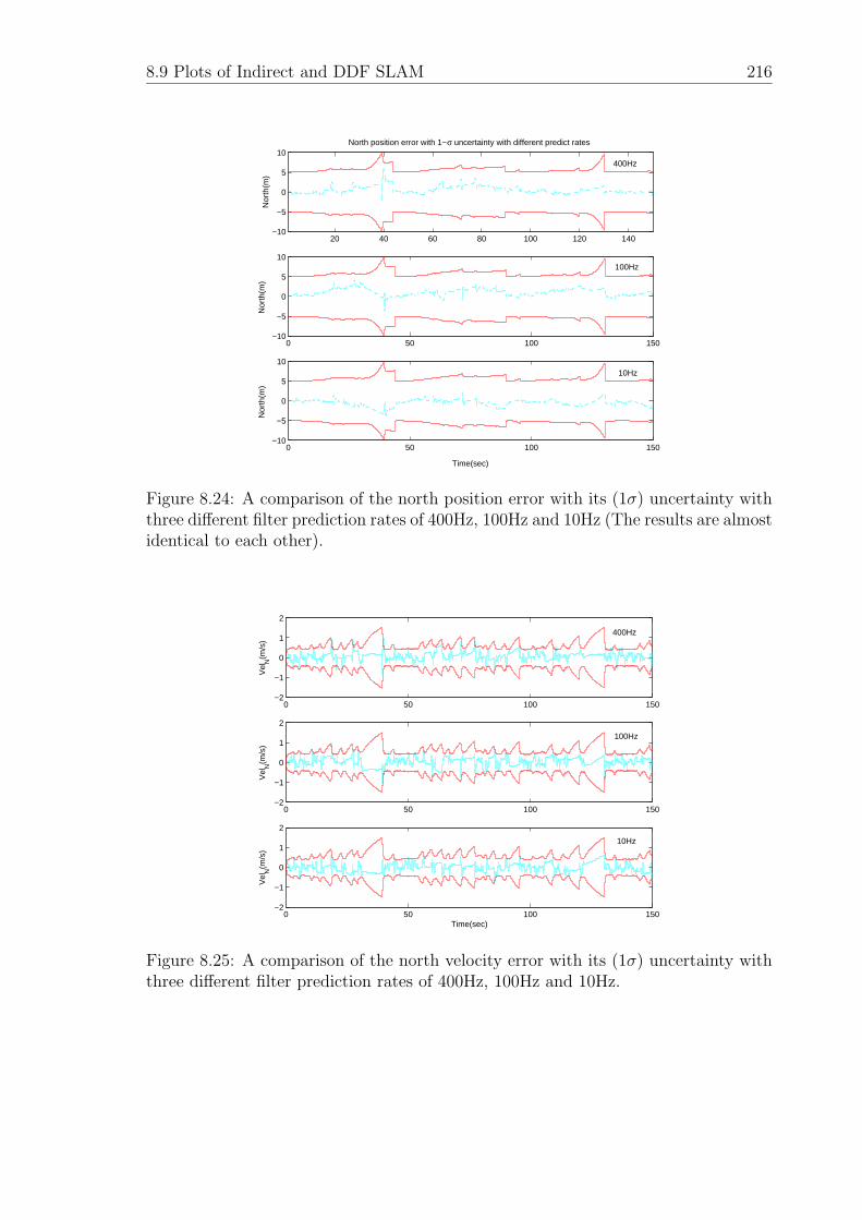
8.9 Plots of Indirect and DDF SLAM 216
20 40 60 80 100 120 140−10
−5
0
5
10
Nor
th(m
)
North position error with 1−σ uncertainty with different predict rates
0 50 100 150−10
−5
0
5
10N
orth
(m)
0 50 100 150−10
−5
0
5
10
Time(sec)
Nor
th(m
)
400Hz
100Hz
10Hz
Figure 8.24: A comparison of the north position error with its (1σ) uncertainty withthree different filter prediction rates of 400Hz, 100Hz and 10Hz (The results are almostidentical to each other).
0 50 100 150−2
−1
0
1
2
Vel
N(m
/s)
0 50 100 150−2
−1
0
1
2
Vel
N(m
/s)
0 50 100 150−2
−1
0
1
2
Vel
N(m
/s)
Time(sec)
400Hz
100Hz
10Hz
Figure 8.25: A comparison of the north velocity error with its (1σ) uncertainty withthree different filter prediction rates of 400Hz, 100Hz and 10Hz.
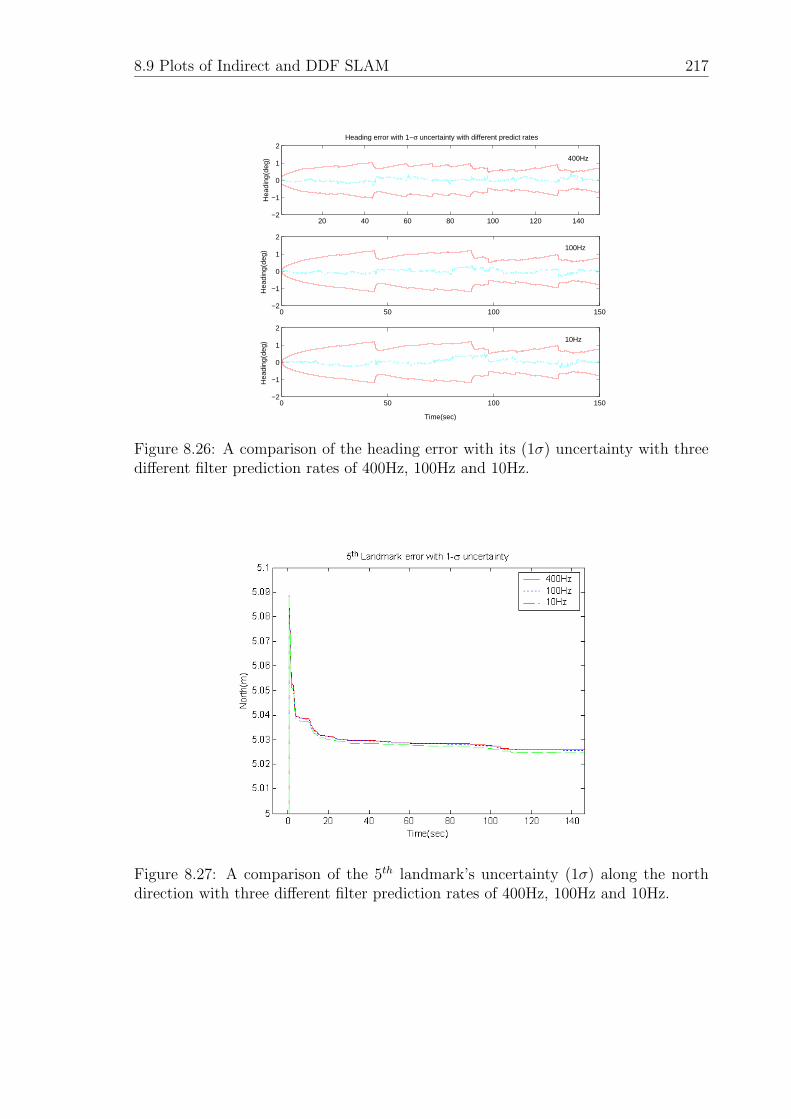
8.9 Plots of Indirect and DDF SLAM 217
20 40 60 80 100 120 140−2
−1
0
1
2Heading error with 1−σ uncertainty with different predict rates
Hea
ding
(deg
)
0 50 100 150−2
−1
0
1
2
Hea
ding
(deg
)
0 50 100 150−2
−1
0
1
2
Hea
ding
(deg
)
Time(sec)
400Hz
100Hz
10Hz
Figure 8.26: A comparison of the heading error with its (1σ) uncertainty with threedifferent filter prediction rates of 400Hz, 100Hz and 10Hz.
Figure 8.27: A comparison of the 5th landmark’s uncertainty (1σ) along the northdirection with three different filter prediction rates of 400Hz, 100Hz and 10Hz.
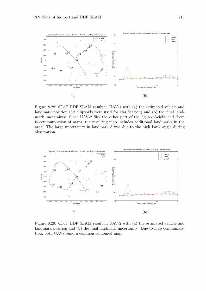
8.9 Plots of Indirect and DDF SLAM 218
−500 −400 −300 −200 −100 0 100 200 300 400 500
−400
−300
−200
−100
0
100
200
300
400
Estimated Vehicle and Landmark Position − Aircraft 1 with Map Communication
1
2
3
4
5 6
7
8 9
10
11
12
13
14
15
North(m)
Eas
t(m
)
SLAMTRUTH
(a)
0 5 10 153
4
5
6
7
8
9Final landmark uncertainty − Aircraft 1 with Map Communication
Unc
erta
inty
of t
arge
t(m
)
Registered Landmark ID
NorthEastDown
(b)
Figure 8.28: 6DoF DDF SLAM result in UAV-1 with (a) the estimated vehicle andlandmark position (5σ ellipsoids were used for clarification) and (b) the final land-mark uncertainty. Since UAV-2 flies the other part of the figure-of-eight and thereis communication of maps, the resulting map includes additional landmarks in thearea. The large uncertainty in landmark 3 was due to the high bank angle duringobservation.
−500 −400 −300 −200 −100 0 100 200 300 400 500
−400
−300
−200
−100
0
100
200
300
400
Estimated Vehicle and Landmark Position − Aircraft 2 with Map Communication
1
2
3
4
5 6
7
8 9
10
11
12
13
14
15
North(m)
Eas
t(m
)
SLAMTRUTH
(a)
0 5 10 153
4
5
6
7
8
9Final landmark uncertainty − Aircraft 2 with Map Communication
Unc
erta
inty
of t
arge
t(m
)
Registered Landmark ID
NorthEastDown
(b)
Figure 8.29: 6DoF DDF SLAM result in UAV-2 with (a) the estimated vehicle andlandmark position and (b) the final landmark uncertainty. Due to map communica-tion, both UAVs build a common combined map.
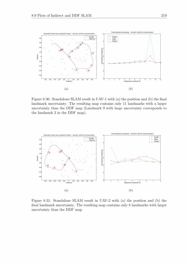
8.9 Plots of Indirect and DDF SLAM 219
−500 −400 −300 −200 −100 0 100 200 300 400 500
−400
−300
−200
−100
0
100
200
300
400
Estimated Vehicle and Landmark Position − Aircraft 1 with No Communication
1
2
3
4 5
6
7
8 9
1011
North(m)
Eas
t(m
)SLAMTRUTH
(a)
0 1 2 3 4 5 6 7 8 9 10 113
4
5
6
7
8
9Final landmark uncertainty − Aircraft 1 with No Communication
Unc
erta
inty
of t
arge
t(m
)
Registered Landmark ID
NorthEastDown
(b)
Figure 8.30: Standalone SLAM result in UAV-1 with (a) the position and (b) the finallandmark uncertainty. The resulting map contains only 11 landmarks with a largeruncertainty than the DDF map (Landmark 9 with large uncertainty corresponds tothe landmark 3 in the DDF map).
−500 −400 −300 −200 −100 0 100 200 300 400 500
−400
−300
−200
−100
0
100
200
300
400
Estimated Vehicle and Landmark Position − Aircraft 2 with No Communication
1
2
345
67
8
North(m)
Eas
t(m
)
SLAMTRUTH
(a)
0 1 2 3 4 5 6 7 83
4
5
6
7
8
9Final landmark uncertainty − Aircraft 2 with No Communication
Unc
erta
inty
of t
arge
t(m
)
Registered Landmark ID
NorthEastDown
(b)
Figure 8.31: Standalone SLAM result in UAV-2 with (a) the position and (b) thefinal landmark uncertainty. The resulting map contains only 8 landmarks with largeruncertainty than the DDF map.
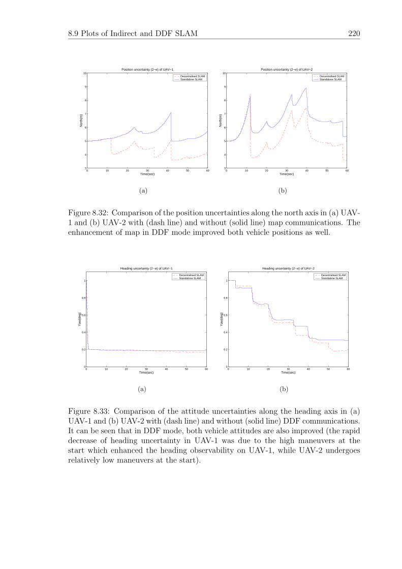
8.9 Plots of Indirect and DDF SLAM 220
0 10 20 30 40 50 603
4
5
6
7
8
9
10
Nor
th(m
)
Time(sec)
Position uncertainty (2−σ) of UAV−1
Decentralised SLAMStandalone SLAM
(a)
0 10 20 30 40 50 603
4
5
6
7
8
9
10
Nor
th(m
)
Time(sec)
Position uncertainty (2−σ) of UAV−2
Decentralised SLAMStandalone SLAM
(b)
Figure 8.32: Comparison of the position uncertainties along the north axis in (a) UAV-1 and (b) UAV-2 with (dash line) and without (solid line) map communications. Theenhancement of map in DDF mode improved both vehicle positions as well.
0 10 20 30 40 50 600
0.2
0.4
0.6
0.8
1
Yaw
(deg
)
Time(sec)
Heading uncertainty (2−σ) of UAV−1
Decentralised SLAMStandalone SLAM
(a)
0 10 20 30 40 50 600
0.2
0.4
0.6
0.8
1
Yaw
(deg
)
Time(sec)
Heading uncertainty (2−σ) of UAV−2
Decentralised SLAMStandalone SLAM
(b)
Figure 8.33: Comparison of the attitude uncertainties along the heading axis in (a)UAV-1 and (b) UAV-2 with (dash line) and without (solid line) DDF communications.It can be seen that in DDF mode, both vehicle attitudes are also improved (the rapiddecrease of heading uncertainty in UAV-1 was due to the high maneuvers at thestart which enhanced the heading observability on UAV-1, while UAV-2 undergoesrelatively low maneuvers at the start).
Chapter 9
Contributions, Conclusion andFuture Research
The focus of this thesis was to develop and demonstrate an autonomous localisa-
tion system for 6DoF UAV platforms. This was achieved by developing the 6DoF
SLAM algorithm using inertial navigation equations as the driving function for the
vehicle model. This expanded the SLAM paradigm to the full 6DoF framework work-
ing within 3D environments, which significantly enhanced the degree of autonomy in
airborne navigation by not relying on any external aiding information like GNSS or
terrain maps. In addition, the 6DoF SLAM algorithm was recast to the indirect struc-
ture which resulted in a more robust and suitable form for real-time implementation
in such environments. Furthermore, the 6DoF SLAM algorithm was also expanded
to the multi-vehicle SLAM domain by using Decentralised Data Fusion (DDF) tech-
niques, which resulted in an improvement to both the map accuracy and the vehicles’
locations. The real-time implementation of this system provided additional contribu-
tions to the engineering knowledge.
The main achievements in this thesis are:
• The development of a 6DoF SLAM algorithm which can autonomously localise
the UAV platform whilst simultaneously building a 3D environment map,
• The development of a computationally efficient 6DoF SLAM algorithm through
Contributions, Conclusion and Future Research 222
the use of the indirect structure,
• An understanding of the effect of sensor field of view to the performance of
SLAM,
• An observability analysis of SLAM which provided a deeper understanding to
its information structure.
• The enhancement of DDF 6DoF SLAM by incorporating the 6DoF model into
the multi-vehicle SLAM problem,
• The real-time implementation of the 6DoF SLAM system for UAV platforms,
• The real-time implementation of a low quality GNSS/Inertial navigation system
for UAV platforms,
• The development of a baro-altimeter aided GNSS/Inertial system to enhance
altitude accuracy whose degradation is normally encountered in highly dynamic
UAVs, and
• The understanding of the error contributions of the lever-arm and vibrations to
the performance of the real system.
Each chapter provided the details of these achievements.
Chapter 3 was concerned with the inertial navigation algorithm which formed a
basis for the airborne application. To estimate the INS error from the filter, the non-
linear INS equations were perturbed and the linearised error equations were obtained.
The lever-arm compensation algorithm was presented and its effects were analysed.
Vibration is an important issue in these types of platforms. It introduces coning
errors to the INS algorithm and degrades the system performance. The effects of the
vibrations and the associated inertial sampling rate were analysed for the real-flight
data and its compensation algorithm was provided. Contributions of this chapter to
this thesis were:
Contributions, Conclusion and Future Research 223
• The development of an INS algorithm in an earth-fixed local-tangent frame.
• The development of an INS error model in an earth-fixed local-tangent frame.
• The analysis of the lever-arm, sampling frequency, and vibration effects in a
real flight environment.
Chapter 4 provided the SLAM algorithm for 6DoF airborne platforms. The
SLAM filter was designed in the EKF framework by using the nonlinear INS and
observation equation. The nonlinear Euler angle equation was used in the filter
prediction and the Jacobians are derived explicitly from that equation. The filter
observation was also performed by using the nonlinear observation model between
the vehicle and landmark. The data association and new feature initialisation in 3D
environment were also formulated. The SLAM algorithm, which is in the direct form,
ran at the sample rate of the IMU data which was 400Hz. Due to its dimensionality
of nine and the high sample rate, the filter prediction computation is not trivial. To
overcome this, the indirect SLAM filter was developed by defining the error as the
filter state. The filter prediction and update was defined on the error dynamic model.
Finally, the SLAM algorithm for a single vehicle was expanded to multiple vehicle
applications by using the information filter in DDF framework. The 6DoF SLAM
algorithm was used as a local filter and the map information is exchanged across the
global information network. Contributions of this chapter were:
• Development of a 6DoF direct SLAM algorithm using a nonlinear vehicle and
observation model.
• Development of a 6DoF indirect (or complementary) SLAM algorithm using a
linearized SLAM error model.
• Development of a decentralised 6DoF SLAM algorithm by using the direct
SLAM as its local filter and using concepts in DDF theory.
Chapter 5 provided the multi-sensor aided inertial navigation algorithms. The
GPS and baro-altimeter sensor were used to observe the INS error from the filter. The
Contributions, Conclusion and Future Research 224
position and velocity solution from the GPS receiver was used as aiding information
which is commonly called a loosely-coupled structure. Although the resulting system
is sub-optimal due to the unknown correlation structure in the GPS solution, it can
greatly reduce the development cycle with enhanced redundancy. In practical airborne
applications, the observation matching is a crucial issue and the timing and spatial
offset between the INS and GPS outputs should be matched precisely to minimise
the observation error. The error contributions were analysed for the real system.
The vulnerability of the GPS vertical channel was addressed, and as a remedy, baro-
altimeter data was augmented to the GNSS/Inertial system for altitude stabilisation.
Contributions of this chapter were:
• The development of a GNSS aided inertial navigation system and an under-
standing of the error contributions in the real system.
• The analysis of the observation matching process to minimise the temporal and
spatial offsets.
• The development of a baro-altimeter augmented GNSS/Inertial navigation sys-
tem.
Chapter 6 provided the details of the hardware and software implementation
of the airborne SLAM system and the GNSS/Inertial system on the Brumby UAV.
The flight vehicle and the sensor systems were presented and the development of
real-time software and the embedded hardware structures were provided in detail.
Contributions of this chapter were:
• The implementation of the GNSS/Inertial navigation system on the Brumby
UAV platform.
• The implementation of the airborne 6DoF SLAM system on the Brumby UAV
platform.
Contributions, Conclusion and Future Research 225
Chapter 7 provided the experiment results of the airborne GNSS/Inertial and
6DoF SLAM navigation systems.
Although the GNSS/Inertial implementation of this system was not the major
contribution of this thesis, it forms the basis for the autonomous guidance and flight
control of the UAV, and the comparison method for the SLAM demonstration. Real-
time results clearly confirmed that the system operates reliably, correcting its inertial
navigation error from the GNSS observation. This system was successfully used in
demonstrating the real-time DDF/feature-tracking on three UAV platforms which
was also recognised as a world first in cooperative UAVs [58]. Additionally, alti-
tude vulnerability of GNSS was observed from real-flight data. To overcome this,
baro-altimeter data was augmented to the GNSS/Inertial system. Off-line processing
results illustrated that the baro-aiding could enhance the height performance partic-
ularly when the UAV underwent frequent banking.
Then the post-processed and real-time SLAM results on the Brumby MK-III plat-
form were presented using an onboard vision sensor and IMU. Although there are
issues for reliable loop closure and the altitude error which resulted from the large
uncertainty in the vision estimate of range, the demonstrations clearly illustrated that
6DoF SLAM in direct form could perform navigation accurately on a UAV platform,
constraining its inertial navigation errors. The results are the first ever flight of real-
time SLAM on a UAV platform using the standard avionic architectures found on
such platforms, and is a substantial contribution of this thesis. Contributions of this
chapter were:
• Real-time demonstration of the GNSS/Inertial system on a UAV platform,
which was successfully used in the guidance/control of a UAV and for feature-
tracking.
• Post-processed results of the baro-altimeter augmented GNSS/Inertial which
showed improved performance in height.
• Post-processed and real-time demonstration of the direct 6DoF SLAM which
Contributions, Conclusion and Future Research 226
showed the success of the airborne SLAM implementation.
Chapter 8 provided further analysis into 6DoF SLAM with the aim of developing
a greater understanding of the algorithm in airborne implementations and to pave
the way for further research.
Firstly, simulated results were presented to verify the direct and indirect form of
6DoF SLAM. It was clearly shown that the indirect form provided almost similar
results to the direct implementation however with significant computational gains.
Secondly, a comparison was conducted between two sensors with different Field of
Views (FOVs) in order to understand the performance differences given these sensors.
The results illustrated that the field-of-view of the environment sensor greatly affected
the localisation performance of the vehicle by providing longer observation time to the
vehicle and hence by constraining the INS error effectively. As part of this analysis
an observability test was conducted, the first of its kind, which demonstrated to what
degree states are observable. In 6DoF SLAM, the degree of observability becomes
either 3N + 5 or 3N + 6 depending on the history of maneuvers, given the dimension
of the system of 3N + 9.
Finally, results of the decentralised SLAM algorithm in a 3D environment were
presented. It illustrated that 6DoF SLAM within the decentralised architecture on
multiple platforms could improve the estimates of both the map and the platform
when compared to the case where platforms performed SLAM independently.
Contributions of this chapter were:
• Simulation results of the 6DoF SLAM algorithms in direct and indirect config-
uration showing that the indirect form can operate in a reduced prediction rate
(10Hz from 400Hz) with comparable performance,
• Simulation results of the decentralised 6DoF SLAM algorithm on two UAV
platforms with improved performance on both of the map and the platform,
Contributions, Conclusion and Future Research 227
• An understanding of the effect of the sensor accuracy and field-of-view on 6DoF
SLAM performance, and
• An observability analysis of SLAM which showed that 6DoF SLAM has three
degrees of rank deficiency.
With this background, ideas for future research will be on the further understand-
ing of the observability of 6DoF SLAM when inertial sensor errors are augmented into
the state vector, in order to improve the integrity and reliability of 6DoF SLAM for
real environment implementations. The aiding of SLAM through the use of a vehicle
dynamic model should also be investigated to constrain the SLAM error for the cases
when extended durations of time of flight occur without any sensor observations. The
focus would be on:
• If the system is completely observable, the ability to estimate the state of SLAM
is dependent on the statistical characteristics of the noise both in the process
and observation model, and the relative geometry between the vehicle and land-
marks. If not, any additional aiding information (including vehicle maneuvers)
that turns the system completely observable should be identified and incorpo-
rated. Otherwise, the 6DoF SLAM filter should be re-designed in a reduced-
order filter by using the observable states to minimise the unnecessary com-
putation. The indirect 6DoF SLAM algorithm can be used effectively for this
observability analysis from the piecewise constant nature of its error model.
• The effects of relative geometry between the vehicle and landmarks in a 3D
environment on the SLAM performance. This is related to the sensitivity of
the SLAM observation matrix and can be studied by analysing the information
contributions from the spatially distributed information sources. Some work
has been done for the optimal configuration of the skewed inertial sensors by
[71], however, SLAM imposes more difficulty due to its complex observation
matrix. By selecting the most informative set of observations for the current
SLAM state, the SLAM efficiency can be enhanced.
Contributions, Conclusion and Future Research 228
• The focus of the work presented in this thesis was on the formulation and
implementation of a 6DoF SLAM system in an airborne environment. Hence,
most of the complexity was directed at the 6DoF algorithm and structure rather
than data association and map management. Indirect 6DoF SLAM developed in
this thesis with map management techniques can greatly increase the efficiency.
This is important in implementing DDF/SLAM on multiple UAVs where the
scale of map can be much larger than the single UAV case. Hence future efforts
should be made into these areas.
• The aiding of an aircraft dynamic model to 6DoF SLAM to enhance the integrity
and reliability when there are no sensor observations for extended time, for
example, due to the lack of the features or due to the difficulty in closing the
loop. In this case, the 6DoF SLAM algorithm will diverge significantly and
hence additional aiding information will be required. Some work has been done
by [47] on aircraft dynamic model aided INS, and its usage to SLAM can enhance
the overall reliability (choosing the next feature to go to will also help although
this can be difficult with fixed wing platforms).
Inertial navigation has been widely used as a means of 6DoF navigation in most
airborne applications. Despite of its advantage being a self-contained system, its un-
bounded error growth has forced it to incorporate external aiding information such
as GNSS, beacon, or a priori terrain map. The aided INS however, becomes greatly
dependant on the signal (or map) availability which restricts the system to operate
in the signal interfered/blocked area such as within a military scenario, or for under-
water systems, or whether on another planet. However, through the use of filtering
techniques, inertial navigation and relative observations, 6DoF SLAM can provide a
means of navigation without relying on any external aiding, whether it is in 2D or
3D environment, or whether it undergoes 3DoF or 6DoF motion.
Bibliography
[1] S. Alban, D.M. Akos, and S.M. Rock. Performance analysis and architectures forins-aided gps tracking loops. In National Technical Meeting, California, UnitedStates, January 2003.
[2] B. Anderson. Optimal Control. Prentice Hall International, Englewood Cliffs,1990.
[3] ARINC Research Corporation. GPS Interface Control Document: ICD-GPS-200C, 1993.
[4] BAE Systems Canada Inc. User’s Manual: Allstar, No. 1200-GEN-0101B, April2000.
[5] W. Baker and R. Clem. Terrain contour matching (TERCOM) premier. NumberASP-TR-77-61. Aeronautical Systems Division, Wright-Patterson, August 1997.
[6] I.Y. Bar-Itzhack. Optimal updating of INS using landmarks. In American Insti-tute of Aeronautics and Astronautics, Inc., pages 492–502, August 1977.
[7] I.Y. Bar-Itzhack and N. Bergman. Control Theoretic Approach to Inertial Nav-igation Systems. Journal of Guidance and Control, 11(3):237–245, 1988.
[8] Y. Bar-Shalom, X. Li, and T. Kirubarajan. Estimation with Applications toTracking and Navigation. John Wiley and Sons, 2001.
[9] D. Benson. A Comparison of Two Approaches to Pure-Inertial and Doppler-Inertial Error Analysis. IEEE Transactions on Aerospace and Electronic Systems,11(4):447–455, July 1975.
[10] J. Bortz. A New Mathematical Formulation for Strapdown Inertial Navigation.IEEE Transactions on Aerospace and Electronic Systems, AES-7(1):61–66, 1971.
[11] K. Britting. Inertial Navigation System Analysis. John Wiley and Sons, Inc,1971.
[12] G. Brooker. Technical Manual: ANSER Radar Node. BAE Systems Australia,2001.
BIBLIOGRAPHY 230
[13] R. Brown and Y. Hwang. Introduction to Random Signals and Applied KalmanFiltering. Wiley, New York, 1992.
[14] J. Castellanos, J. Montiel, and J. Tardos. Sensor Influence in the Performanceof Simultaneous Mobile Robot Localization and Map Building. ExperimentalRobotics, IV, 2000.
[15] A. Chatfield. Fundamentals of High Accuracy Inertial Guidance. American In-stitute of Aeronautics and Astronautics, Inc, 1997.
[16] M. Csorba. Simultaneous Localisation and Map Building. PhD thesis, AustralianCentre for Field Robotics, The University of Oxford, 1997.
[17] J. Dezert and C. Hailey. Multitarget-Multisensor Tracking: Applications andAdvances, volume 2, chapter Autonomous navigation with uncertain referencepoints using the PDAF. 1992.
[18] M. Dissanayake, P. Newman, H. Durrant-Whyte, S. Clark, and M. Csorba. Anexperimental and theoretical investigation into simultaneous localisation andmap building. Experimental Robotics, IV:265–274, 2000.
[19] M. Dissanayake, P. Newman, H. Durrant-Whyte, S. Clark, and M. Csorba. Asolution to the simultaneous localisation and map building problem. IEEE Trans-actions on Robotics and Automation, 17(3):229–241, June 2001.
[20] R. Duda and P. Hart. Pattern Classification and Scene Analysis. John Wileyand Sons, 1973.
[21] European Commission. The GALILEI Project: GALILEO Design Consolidation,2003.
[22] N. Gordon, D. Salmond, and A. Smith. Novel approach to nonlinear/non–Gaussian Bayesian state estimation. In IEE Proceedings-F, pages 107–113, 1993.
[23] D. Goshen-Meskin and I.Y. Bar-Itzhack. Observability Analysis of Piece-wiseConstant Systems-Part I: Theory. IEEE Transactions on Aerospace and Elec-tronic Systems, 28(4):1056–1067, 1992.
[24] D. Goshen-Meskin and I.Y. Bar-Itzhack. Unified Approach to Inertial Navi-gation System Error Modelling. Journal of Guidance, Control, and Dynamics,15(3):648–653, May-June 1992.
[25] R. Greenspan. GPS and Inertial Navigation, chapter 7. American Institute ofAeronautics and Astronautics, Inc, 1996.
[26] J. Guivant and E. Nebot. Optimization of the simultaneous localisation and mapbuilding algorithm for real-time implementation. IEEE Transactions on Roboticsand Automation, 17(3):242–257, 2001.
BIBLIOGRAPHY 231
[27] A. Henley. Terrain aided navigation: current status, techniques for flat terrainand reference data requirements. In IEEE Position Location and NavigationSymposium, pages 608–615, March 1990.
[28] L. Hostetler and R. Beckmann. Nonlinear Kalman filtering techniques for terrain-aided navigation. pages 315–323, march 1983.
[29] M. Ignagni. Efficient Class of Optimized Coning Compensation Algorithm. Jour-nal of Guidance, Control, and Dynamics, 19(2):424–429, March-April 1996.
[30] M. Ignagni. Duality of Optimal Strapdown Sculling and Coning CompensationAlgorithms. Journal of the ION, 45(2), Summer 1998.
[31] Inertial Science Inc. Technical Manual: Inertial Measurement Unit, ISIS Rev.C,1999.
[32] Integrated Systems Inc. Developing pSOSystem Applications Version 2.22, 1998.
[33] Inter-Governmental Committee on Surveying and Mapping. Geocentric Datumof Australia Technical Manual Version 2.2 .
[34] Snyder J. Map Projections used by the U.S. Geological Survey. United Statesof America Department of Interior, U.S. Geological Survey Bulletin 1532, 2ndEdition, 1984.
[35] I. Jung and S. Lacroix. High resolution terrain mapping using low altitudeaerial stereo imagery. In The Ninth IEEE International Conference on ComputerVision, 2003.
[36] E.D. Kaplan. Understanding GPS: Principles and Applications. Artech House,Inc., 1996.
[37] J. Kim, S. W. Moon, S. H. Kim, D. H. Hwang, S. J. Lee, M. S. Oh, and S. W. Ra.Design of a loosely-coupled GPS/INS integration system. Journal of the KoreaInstitute of Military Science and Technology, 2(2):186–196, December 1999.
[38] J. Kim, S. W. Moon, S. H. Lee, S. H. Kim, D. H. Hwang, S. J. Lee, and S. W.Ra. Implementation of an Initial Alignment Algorithm for a Strapdown InertialNavigation System. Journal of Institute of Control, Automation and SystemsEngineering, Korea, 6(2):138–145, February 2000.
[39] J. Kim, Sharon Ong, E. Nettleton, and S. Sukkarieh. Decentralised approachto UAV navigation: without the use of GPS and preloaded maps. Journal ofAerospace Engineering, In press.
BIBLIOGRAPHY 232
[40] J. Kim and S. Sukkarieh. Flight Test Results of GPS/INS Navigation Loop foran Autonomous Unmanned Aerial Vehicle (UAV). In International TechnicalMeeting of the Satellite Division of the Institute of Navigation (ION), pages510–517, Portland, OR, USA, September 2002.
[41] J. Kim and S. Sukkarieh. Airborne Simultaneous Localisation and Map Building.In IEEE International Conference on Robotics and Automation, Taipei, Taiwan,2003.
[42] J. Kim and S. Sukkarieh. Recasting SLAM - Towards Improving Efficiencyand Platform Independency. In International Symposium on Robotics Research,Siena, Italy, 2003.
[43] J. Kim and S. Sukkarieh. Autonomous Airborne Navigation in Unknown Ter-rain Environments. IEEE Transactions on Aerospace and Electronic Systems,40(3):1031–1045, July 2004.
[44] J. Kim and S. Sukkarieh. Improving the Real-Time Efficiency of Inertial SLAMand Understanding its Observability. In IEEE/RSJ International Conference onIntelligent Robots and Systems, Sendai, Japan, 2004.
[45] J. Kim, S. Sukkarieh, E. Nebot, and J. Guivant. On the Effects of using Head-ing Information during In-flight Alignment of a Low-cost IMU/GPS IntegratedSystem. In International Conference of Field and Service Robotics, pages 55–60,Helsinki, Finland, June 2001.
[46] J. Kim, S. Sukkarieh, and S. Wishart. Real-time Navigation, Guidance andControl of a UAV using Low-cost Sensors. In International Conference of Fieldand Service Robotics, pages 95–100, Yamanashi, Japan, July 2003.
[47] M. Koifman and I.Y. Bar-Itzhack. Inertial Navigation System Aided by AircraftDynamics. Journal of Guidance and Control, 7(4):487–493, 1999.
[48] J. G. Lee, Y. J. Yoon, J. G. Mark, and D. A. Tazartes. Extension of Strap-down Attitude Algorithm for High-Frequency Base Motion. Journal of DynamicSystems, Measurement and Control, 13(4):738–743, 1990.
[49] J. Leonard and H. Feder. Experimental analysis of adaptive concurrent mappingand localisation using sonar. International Symposium on Experimental Robotics,1999.
[50] S. Majumder. Sensor Fusion and Feature Based Navigation for Subsea Robots.PhD thesis, Australian Centre for Field Robotics, The University of Sydney,2001.
[51] P. Maybeck. Stochastic Models, Estimations and Control, volume 1,2. AcademicPress, 1982.
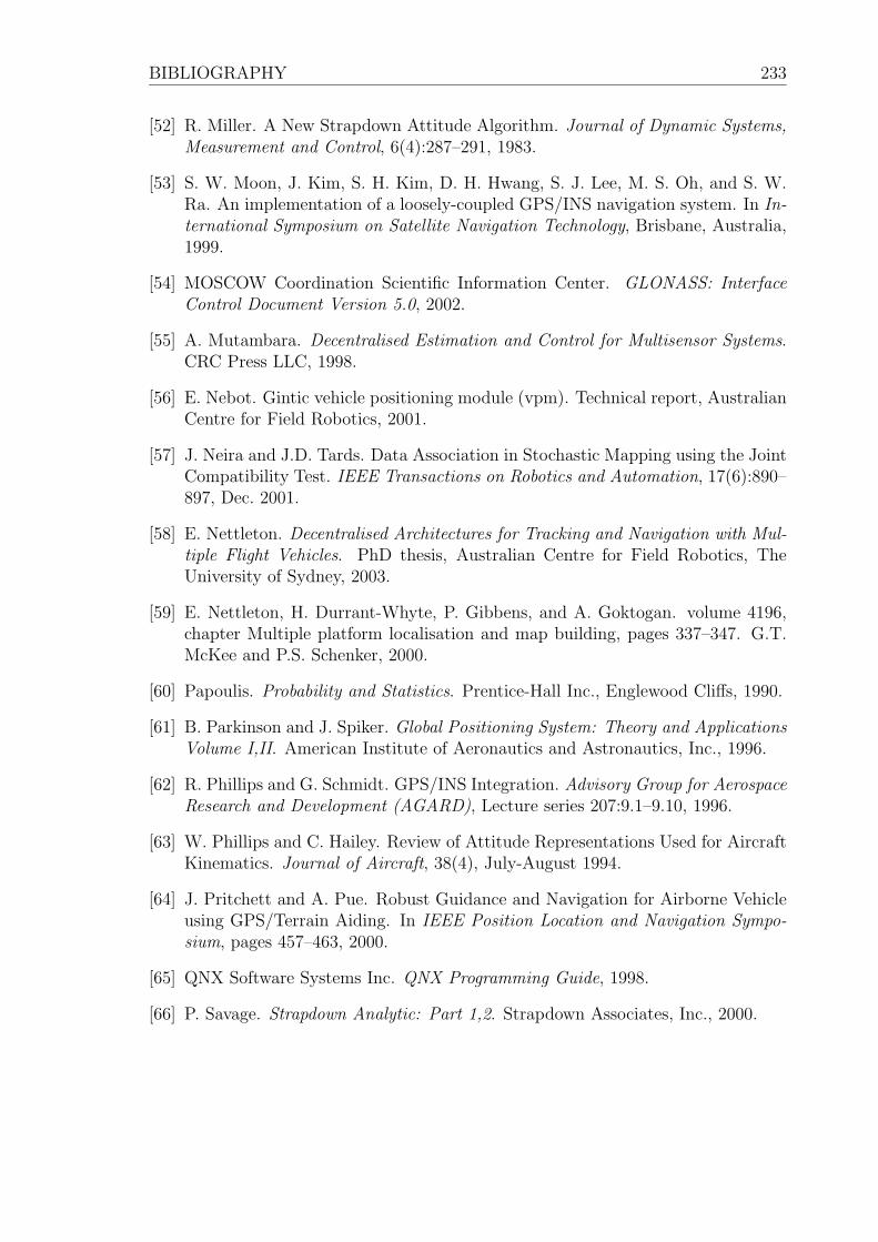
BIBLIOGRAPHY 233
[52] R. Miller. A New Strapdown Attitude Algorithm. Journal of Dynamic Systems,Measurement and Control, 6(4):287–291, 1983.
[53] S. W. Moon, J. Kim, S. H. Kim, D. H. Hwang, S. J. Lee, M. S. Oh, and S. W.Ra. An implementation of a loosely-coupled GPS/INS navigation system. In In-ternational Symposium on Satellite Navigation Technology, Brisbane, Australia,1999.
[54] MOSCOW Coordination Scientific Information Center. GLONASS: InterfaceControl Document Version 5.0, 2002.
[55] A. Mutambara. Decentralised Estimation and Control for Multisensor Systems.CRC Press LLC, 1998.
[56] E. Nebot. Gintic vehicle positioning module (vpm). Technical report, AustralianCentre for Field Robotics, 2001.
[57] J. Neira and J.D. Tards. Data Association in Stochastic Mapping using the JointCompatibility Test. IEEE Transactions on Robotics and Automation, 17(6):890–897, Dec. 2001.
[58] E. Nettleton. Decentralised Architectures for Tracking and Navigation with Mul-tiple Flight Vehicles. PhD thesis, Australian Centre for Field Robotics, TheUniversity of Sydney, 2003.
[59] E. Nettleton, H. Durrant-Whyte, P. Gibbens, and A. Goktogan. volume 4196,chapter Multiple platform localisation and map building, pages 337–347. G.T.McKee and P.S. Schenker, 2000.
[60] Papoulis. Probability and Statistics. Prentice-Hall Inc., Englewood Cliffs, 1990.
[61] B. Parkinson and J. Spiker. Global Positioning System: Theory and ApplicationsVolume I,II. American Institute of Aeronautics and Astronautics, Inc., 1996.
[62] R. Phillips and G. Schmidt. GPS/INS Integration. Advisory Group for AerospaceResearch and Development (AGARD), Lecture series 207:9.1–9.10, 1996.
[63] W. Phillips and C. Hailey. Review of Attitude Representations Used for AircraftKinematics. Journal of Aircraft, 38(4), July-August 1994.
[64] J. Pritchett and A. Pue. Robust Guidance and Navigation for Airborne Vehicleusing GPS/Terrain Aiding. In IEEE Position Location and Navigation Sympo-sium, pages 457–463, 2000.
[65] QNX Software Systems Inc. QNX Programming Guide, 1998.
[66] P. Savage. Strapdown Analytic: Part 1,2. Strapdown Associates, Inc., 2000.
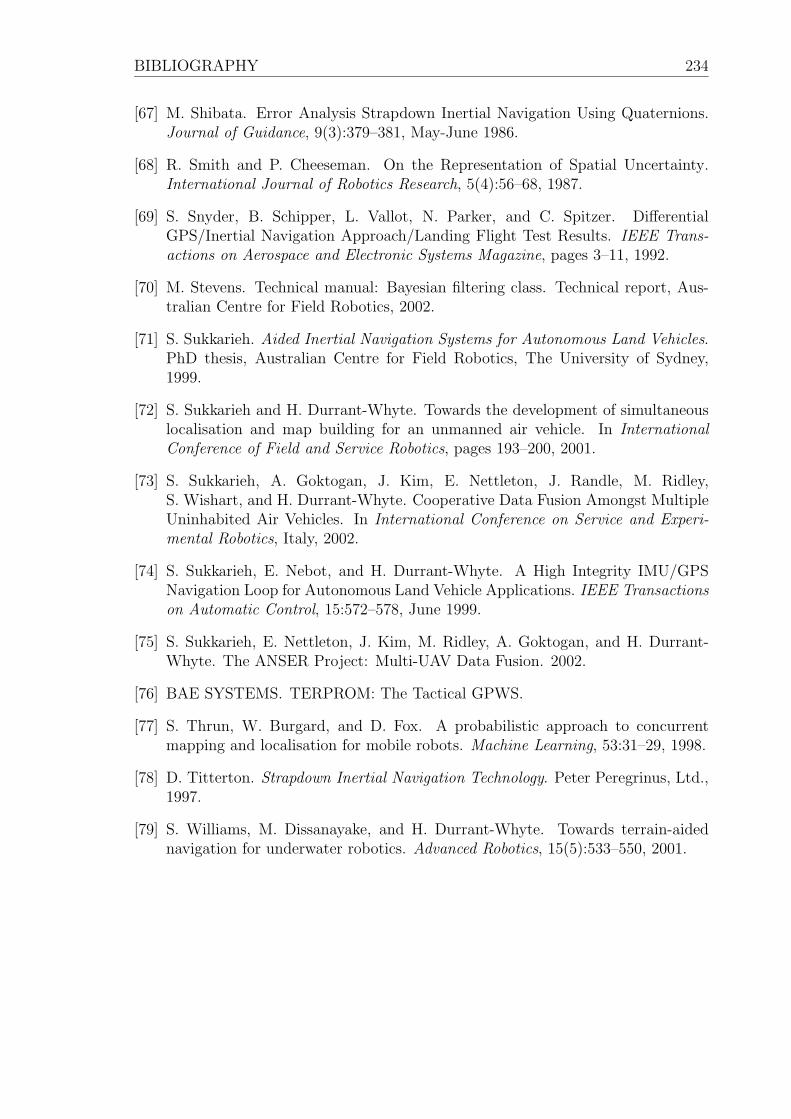
BIBLIOGRAPHY 234
[67] M. Shibata. Error Analysis Strapdown Inertial Navigation Using Quaternions.Journal of Guidance, 9(3):379–381, May-June 1986.
[68] R. Smith and P. Cheeseman. On the Representation of Spatial Uncertainty.International Journal of Robotics Research, 5(4):56–68, 1987.
[69] S. Snyder, B. Schipper, L. Vallot, N. Parker, and C. Spitzer. DifferentialGPS/Inertial Navigation Approach/Landing Flight Test Results. IEEE Trans-actions on Aerospace and Electronic Systems Magazine, pages 3–11, 1992.
[70] M. Stevens. Technical manual: Bayesian filtering class. Technical report, Aus-tralian Centre for Field Robotics, 2002.
[71] S. Sukkarieh. Aided Inertial Navigation Systems for Autonomous Land Vehicles.PhD thesis, Australian Centre for Field Robotics, The University of Sydney,1999.
[72] S. Sukkarieh and H. Durrant-Whyte. Towards the development of simultaneouslocalisation and map building for an unmanned air vehicle. In InternationalConference of Field and Service Robotics, pages 193–200, 2001.
[73] S. Sukkarieh, A. Goktogan, J. Kim, E. Nettleton, J. Randle, M. Ridley,S. Wishart, and H. Durrant-Whyte. Cooperative Data Fusion Amongst MultipleUninhabited Air Vehicles. In International Conference on Service and Experi-mental Robotics, Italy, 2002.
[74] S. Sukkarieh, E. Nebot, and H. Durrant-Whyte. A High Integrity IMU/GPSNavigation Loop for Autonomous Land Vehicle Applications. IEEE Transactionson Automatic Control, 15:572–578, June 1999.
[75] S. Sukkarieh, E. Nettleton, J. Kim, M. Ridley, A. Goktogan, and H. Durrant-Whyte. The ANSER Project: Multi-UAV Data Fusion. 2002.
[76] BAE SYSTEMS. TERPROM: The Tactical GPWS.
[77] S. Thrun, W. Burgard, and D. Fox. A probabilistic approach to concurrentmapping and localisation for mobile robots. Machine Learning, 53:31–29, 1998.
[78] D. Titterton. Strapdown Inertial Navigation Technology. Peter Peregrinus, Ltd.,1997.
[79] S. Williams, M. Dissanayake, and H. Durrant-Whyte. Towards terrain-aidednavigation for underwater robotics. Advanced Robotics, 15(5):533–550, 2001.