Embed Size (px)
Citation preview
Benchmarking OpenVG implementations
–
Paint performances of a
2D vector graphics hardware accelerated API
–
JEROME
FRANCISCO
DUBOIS GARCIA
Academic project. Supervisor: LETIZIA JACCHERI. Autumn 2006

Benchmarking OpenVG implementations Jerome Dubois and Francisco Garcia
Autumn 2006 Page 2/114
– Blank page –

Benchmarking OpenVG implementations Jerome Dubois and Francisco Garcia
Autumn 2006 Page 3/114
ACKNOWLEDGMENT
We have appreciated working and collaborating with the other stakeholders, so we wish to thank them. First, our thanks go to our supervisor Letizia Jaccheri for her valuable advices and feedbacks concerning the way to conduct the project.
We would also like to thank Mario Blazevic from ARM, for proposing the project and providing technical feedbacks. We would like to extend our thanks to Espen and Thomas, from ARM, for their OpenVG demonstration and review of the test’s concepts.
We have appreciated to collaborate with Brice and thank him for his help, especially for helping us to start the project.

Benchmarking OpenVG implementations Jerome Dubois and Francisco Garcia
Autumn 2006 Page 4/114
PREAMBLE
This document is the report of a university project carried out by two students: Jerome Dubois and Francisco Garcia.
We are students in semester 9 (5th year) in a Master curriculum:
University NTNU: Norwegian University of Science and Technology Location Trondheim, Norway Faculty Faculty of Information technology, Mathematics and Electrical engineering
(IME) Department Department of Computer and Information Science (IDI)
This project is a 15 ECTS (European Credit) project, and has been carried out during one semester, witch means that it took half of our study (One semester is 30 ECTS). It was carried out from September 2006 to December 2006.
This project is supervised by a NTNU teacher:
! Mrs. Letizia Jaccheri ([email protected]) (http://www.idi.ntnu.no/~letizia/)
This project has been carried out in collaboration with ARM Norway (http://www.falanx.no/).
We are both foreign students at the NTNU, as part of exchanges programs between universities.
! Jerome Dubois comes from University INPG (http://www.inpg.fr/): Grenoble Institute of Technology School ENSIMAG (http://www.ensimag.fr/):
French engineering school of “IT and applied mathematics” of Grenoble Location Grenoble, France
! Francisco Garcia comes from University University of Murcia (www.um.es) Faculty Faculty of informatics (www.um.es/informatica) Location Murcia, Spain
Benchmarking OpenVG implementations Jerome Dubois and Francisco Garcia
Autumn 2006 Page 5/114
ABSTRACT .
The portable device domain is going to change with the arrival of OpenVG, a graphical API for hardware accelerated 2D vector graphics. Introduced by the Khronos Group, this API allows the graphic application developers to abstract the hardware while beneficiating good performance due to the use of a GPU and hardware acceleration.
OpenVG deals with paths, paints, and images, and offers a set of useful transformations and options.
The project consists in creating a benchmark for OpenVG implementations.
Benchmarking is a delicate task, though important when considering performances. It deals with evaluating a system, most of the time to compare it with concurrent systems.
We have designed, implemented and run a first draft benchmark, to gain the basics of benchmarking OpenVG.
Then, we have worked on a second iteration in which the benchmark measures Paint performances of OpenVG implementations, based on a pixel per second metric.
The framework of the benchmark can be reused easily for similar projects.
Benchmarking OpenVG implementations Jerome Dubois and Francisco Garcia
Autumn 2006 Page 6/114
TABLE OF CONTENT
Acknowledgment ...................................................................................................................... 3 Preamble ................................................................................................................................... 4 Abstract . ................................................................................................................................... 5 Table of content ........................................................................................................................ 6 Table of figures ....................................................................................................................... 10 1. Introduction ............................................................................................................ 11
1.1. Motivation................................................................................................................ 11 1.2. Vector graphic ......................................................................................................... 12 1.3. Portable devices ....................................................................................................... 12 1.4. Benchmark............................................................................................................... 13 1.5. Structure of the work............................................................................................... 13
Part I. Project .......................................... 14 2. Context of our work ............................................................................................... 15
2.1. Place of this project in our education..................................................................... 15 2.2. Stakeholders............................................................................................................. 15 2.3. Environment ............................................................................................................ 15 2.4. Release ..................................................................................................................... 16
3. Researching work................................................................................................... 17 3.1. Task: definition and evolution................................................................................ 17 3.2. Reflections about the researching work ................................................................. 17 3.3. Plan .......................................................................................................................... 19 3.4. Research Goals and questions ................................................................................ 19 3.5. Practical goals ......................................................................................................... 19
4. State of the Art........................................................................................................ 21 4.1. OpenVG literature and code review........................................................................ 21 4.2. OpenVG implementations review ........................................................................... 22 4.3. Benchmark literature review................................................................................... 22
Part II. Study ........................................... 23
5. OpenVG................................................................................................................... 24 5.1. The ideal pipeline .................................................................................................... 24
5.1.1. Stage 1: Path, Transformation, Stroke and Paint ............................................ 24 5.1.2. Stage 2: Stroked Path Generation.................................................................... 25 5.1.3. Stage 3: Transformation................................................................................... 25 5.1.4. Stage 4: Rasterization ...................................................................................... 25 5.1.5. Stage 5: Clipping and Masking........................................................................ 25 5.1.6. Stage 6: Paint Generation................................................................................ 26
Benchmarking OpenVG implementations Jerome Dubois and Francisco Garcia
Autumn 2006 Page 7/114
5.1.7. Stage 7: Image Interpolation............................................................................ 26 5.1.8. Stage 8: Blending and Antialiasing.................................................................. 26
5.2. OpenVG and EGL ................................................................................................... 27 5.2.1. Layer organization of an OpenVG framework................................................. 27 5.2.2. From EGL to the screen ................................................................................... 28 5.2.3. OpenVG collaborating with others APIs ......................................................... 29 5.2.4. EGL provides a drawing context...................................................................... 29
5.3. General Notions....................................................................................................... 30 5.3.1. OpenVG Objects: handles. ............................................................................... 30 5.3.2. OpenVG parameters......................................................................................... 31 5.3.3. Handle parameters ........................................................................................... 32 5.3.4. Coordinate systems and transformations......................................................... 32 5.3.5. All OpenVG parameters ................................................................................... 33
5.4. Transformations ...................................................................................................... 33 5.4.1. When do the transformations occur? ............................................................... 33 5.4.2. Homogeneous coordinates and transformation matrixes ................................ 34 5.4.3. Affine transformations explained ..................................................................... 34 5.4.4. Matrix manipulations ....................................................................................... 38 5.4.5. Matrix functions ............................................................................................... 40 5.4.6. Benefit of hardware accelerated transformation ............................................. 41
5.5. Colors ....................................................................................................................... 42 5.5.1. Color spaces..................................................................................................... 42 5.5.2. Premultiplied and non-premultiplied color values .......................................... 44 5.5.3. Colors in OpenVG............................................................................................ 44
5.6. Gradients.................................................................................................................. 45 5.6.1. Linear Gradients .............................................................................................. 45 5.6.2. Radial Gradients .............................................................................................. 45 5.6.3. Color Ramps..................................................................................................... 46
5.7. Paths......................................................................................................................... 47 5.7.1. What is a path................................................................................................... 47 5.7.2. Segment commands .......................................................................................... 49 5.7.3. Paths operations and capabilities .................................................................... 49 5.7.4. Stroking a path ................................................................................................. 50 5.7.5. Filling a path.................................................................................................... 51 5.7.6. Example of code ............................................................................................... 53 5.7.7. All explicit and implicit parameters of a path.................................................. 53 5.7.8. Paths functions ................................................................................................. 54
5.8. Paints ....................................................................................................................... 55 5.8.1. Binding Paint to the context ............................................................................. 55 5.8.2. Paint parameters .............................................................................................. 56 5.8.3. Paint functions.................................................................................................. 57
5.9. Images...................................................................................................................... 57 5.9.1. Modifying Image pixels .................................................................................... 59 5.9.2. Image filters...................................................................................................... 59 5.9.3. Image functions ................................................................................................ 60
5.10. Conclusions ............................................................................................................. 61 6. Benchmarking......................................................................................................... 62
Benchmarking OpenVG implementations Jerome Dubois and Francisco Garcia
Autumn 2006 Page 8/114
6.1. Definition and Goals of benchmarking.................................................................. 62 6.1.1. Definition of Benchmarking ............................................................................. 62 6.1.2. Goals of Benchmarking.................................................................................... 62 6.1.3. Need for a reference......................................................................................... 63 6.1.4. Performance evaluation and Benchmarking.................................................... 63
6.2. Neutral point of view and benchmark business ..................................................... 63 6.3. Metrics ..................................................................................................................... 64
6.3.1. Characteristics of a good performance metric ................................................ 64 6.3.2. Example of metrics ........................................................................................... 65 6.3.3. Speedup and relative change............................................................................ 66
6.4. Measurements.......................................................................................................... 67 6.5. Benchmark programs.............................................................................................. 69
6.5.1. Types of benchmark applications..................................................................... 69 6.5.2. Strategies for benchmark applications............................................................. 71 6.5.3. Amdahl’s law.................................................................................................... 72
6.6. Computing performances into a single number..................................................... 73 6.6.1. Different means ................................................................................................ 73 6.6.2. Choice of the method........................................................................................ 74 6.6.3. Think about....................................................................................................... 74 6.6.4. Statistical dispersion ........................................................................................ 74
6.7. Interpretation and use of the data measured ......................................................... 75 Part III. Benchmark documentation...... 76
7. Benchmark – Specifications .................................................................................. 77 7.1. Metrics and measurement issues ............................................................................ 77
7.1.1. Metrics.............................................................................................................. 77 7.1.2. Test repetition and result.................................................................................. 77 7.1.3. Overview of the process from measurement to final mark............................... 79 7.1.4. Combination of all test’s measurements for the test result .............................. 79 7.1.5. Combination of all tests results for the final mark........................................... 81
7.2. Portability issues...................................................................................................... 86 7.3. Output of the benchmark ........................................................................................ 86
7.3.1. Choice of the information for the output.......................................................... 86 7.3.2. Output format ................................................................................................... 87 7.3.3. Dumping frame buffer ...................................................................................... 88
7.4. User’s manual.......................................................................................................... 88 8. Benchmark – Architecture .................................................................................... 90
8.1. Random Number Generator ................................................................................... 90 8.2. Files.......................................................................................................................... 91
8.2.1. vgb06_header.h ................................................................................................ 91 8.2.2. main.cpp ........................................................................................................... 93 8.2.3. vgb06_main.cpp ............................................................................................... 94 8.2.4. Test files............................................................................................................ 95
9. Benchmark – Test design....................................................................................... 96 9.1. Categories of features.............................................................................................. 96
Benchmarking OpenVG implementations Jerome Dubois and Francisco Garcia
Autumn 2006 Page 9/114
9.2. Identifying appropriate parameters ........................................................................ 97 9.2.1. Parameter A: Opacity ...................................................................................... 97 9.2.2. Parameter B: Number of color stops ............................................................... 97 9.2.3. Parameter C: Ramp spread mode.................................................................... 97 9.2.4. Parameter D: Paint type .................................................................................. 98 9.2.5. Parameter E: Blending mode........................................................................... 98 9.2.6. Parameter F: Paint transformations................................................................ 98 9.2.7. Parameter G: Surface affected......................................................................... 99 9.2.8. General parameters.......................................................................................... 99
9.3. Tests architecture .................................................................................................... 99 10. Benchmark – Test implementation..................................................................... 101
10.1. Macros for parameter values ................................................................................ 101 10.2. Main function ........................................................................................................ 102 10.3. Paths generation.................................................................................................... 103 10.4. Paint generation .................................................................................................... 103 10.5. SeTting blending modes and Paint transformations ........................................... 104 10.6. Skipping parameter combinations ........................................................................ 105 10.7. Performing the tests............................................................................................... 105
11. Conclusion............................................................................................................. 107 11.1. What is not finished?............................................................................................. 107
11.1.1. About the benchmark...................................................................................... 107 11.1.2. About the report ............................................................................................. 108
11.2. Future benchmarks ............................................................................................... 109 11.3. Evaluation of the benchmark................................................................................ 109 11.4. Evaluation of the project ....................................................................................... 110
Bibliography ......................................................................................................................... 111 Annexes . ............................................................................................................................... 114
A. Annex: a SVG example ......................................................................................... 114 B. Annex: vector graphic and mapping application................................................. 114
Benchmarking OpenVG implementations Jerome Dubois and Francisco Garcia
Autumn 2006 Page 10/114
TABLE OF FIGURES
Figure 1: Tiger example ........................................................................................................... 21 Figure 2: OpenVG environment............................................................................................... 28 Figure 3: VGHandle ................................................................................................................. 31 Figure 4: Drawing surface........................................................................................................ 33 Figure 5: Formula for affine transformation ............................................................................ 35 Figure 6: Formula of rotation transformation .......................................................................... 38 Figure 7: additive colors........................................................................................................... 42 Figure 8: sRGB space color ..................................................................................................... 43 Figure 9: linear gradient ........................................................................................................... 45 Figure 10: radial gradient description ...................................................................................... 46 Figure 11: radial gradient ......................................................................................................... 46 Figure 12: color ramp............................................................................................................... 47 Figure 13: cross ........................................................................................................................ 47 Figure 14: detailed Path for drawing a cross............................................................................ 48 Figure 15: Filling: initial Path .................................................................................................. 51 Figure 16: Filling: assigning a number to areas ....................................................................... 51 Figure 17: Time intervals ......................................................................................................... 69 Figure 18: Amdal's law formula............................................................................................... 72 Figure 19: Amdal's law ............................................................................................................ 72
Benchmarking OpenVG implementations Jerome Dubois and Francisco Garcia
Autumn 2006 Page 11/114
1. INTRODUCTION
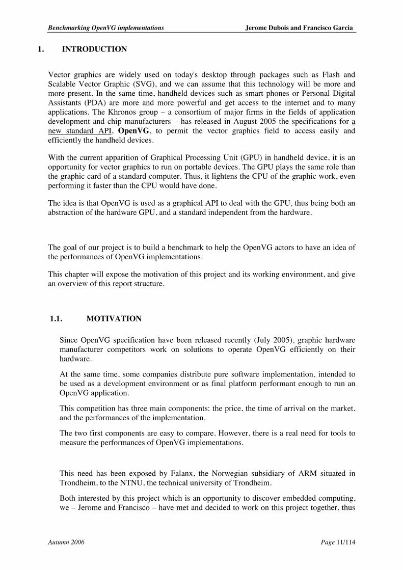
Vector graphics are widely used on today's desktop through packages such as Flash and Scalable Vector Graphic (SVG), and we can assume that this technology will be more and more present. In the same time, handheld devices such as smart phones or Personal Digital Assistants (PDA) are more and more powerful and get access to the internet and to many applications. The Khronos group – a consortium of major firms in the fields of application development and chip manufacturers – has released in August 2005 the specifications for a new standard API, OpenVG, to permit the vector graphics field to access easily and efficiently the handheld devices.
With the current apparition of Graphical Processing Unit (GPU) in handheld device, it is an opportunity for vector graphics to run on portable devices. The GPU plays the same role than the graphic card of a standard computer. Thus, it lightens the CPU of the graphic work, even performing it faster than the CPU would have done.
The idea is that OpenVG is used as a graphical API to deal with the GPU, thus being both an abstraction of the hardware GPU, and a standard independent from the hardware.
The goal of our project is to build a benchmark to help the OpenVG actors to have an idea of the performances of OpenVG implementations.
This chapter will expose the motivation of this project and its working environment, and give an overview of this report structure.
1.1. MOTIVATION
Since OpenVG specification have been released recently (July 2005), graphic hardware manufacturer competitors work on solutions to operate OpenVG efficiently on their hardware.
At the same time, some companies distribute pure software implementation, intended to be used as a development environment or as final platform performant enough to run an OpenVG application.
This competition has three main components: the price, the time of arrival on the market, and the performances of the implementation.
The two first components are easy to compare. However, there is a real need for tools to measure the performances of OpenVG implementations.
This need has been exposed by Falanx, the Norwegian subsidiary of ARM situated in Trondheim, to the NTNU, the technical university of Trondheim.
Both interested by this project which is an opportunity to discover embedded computing, we – Jerome and Francisco – have met and decided to work on this project together, thus
Benchmarking OpenVG implementations Jerome Dubois and Francisco Garcia
Autumn 2006 Page 12/114
going further than if it was a single project, while keeping the opportunity for each of us to understand the whole project.
Due to the youngness of OpenVG, the literature and code samples are few. We hope our work will help people interested in OpenVG to have a first global understanding of it, before going through the specifications or other reading.
1.2. VECTOR GRAPHIC
“Vector graphics is the use of geometrical primitives such as points, lines, curves, and polygons, which are all based upon mathematical equations to represent images in computer graphics. It is used by contrast to the term raster graphics, which is the representation of images as a collection of pixels.”[B11]
The most known advantage of vector graphics is that one can zoom infinity and still have smooth shapes, whereas with raster graphic the pixels are distinguishable.
To draw a circle in vector graphic, the order is “Draw a circle of radius r and center (x,y) in red with a width of 1mm”. In raster graphic, every pixel to be drawn has to be described.
The information stored in a vector graphic format occupies less space. On the other hand, a vector graphic viewer takes more time to compute the image to be drawn.
Yet another benefit of vector graphic is that it is much more practical for some applications to deal with graphical objects (circle, lines), since a lot of transformations can be applied to them before drawing.
1.3. PORTABLE DEVICES
Mobile devices are a quick growing field. These are not only mobile telephones but smart phones or Personal Digital Assistants (PDA), with an advanced operating system and graphic interface. Their use has been growing and they provide more and more function and application.
As their capacities were high enough to run bigger software, we saw the same problem than for computers before the apparition of graphic cards. Then, the GPU, Graphical Process Unit, arrived in mobile devices to help the CPU, Central Process Unit, to deal with the graphic aspects. This provides more efficient ways to compute graphic, since GPU have been designed on this specific purpose, whereas CPU are for general applications. At the same time, this lightens the CPU task, permitting it to concentrate on other jobs. It also uses less power, which is a challenge in portable devices world.
With the apparition of multimedia on mobile devices, and the growth of their screen, efficient ways of dealing graphics had to be founded. Khronos, a consortium of major graphic actors of the market, has then designed a solution with OpenGL ES, a 2D-3D graphic API for embedded systems, which is a subset of desktop OpenGL API. This API is a success, and within four years, it has become the standard for embedded accelerated 3D Graphics [khronos.org].
Benchmarking OpenVG implementations Jerome Dubois and Francisco Garcia
Autumn 2006 Page 13/114
As we have seen before, vector graphics are very much better to use for some applications. As there is a need for it on embedded devices, Khronos decided to deliver another API, OpenVG, to deal with 2D vector graphics.
The applications which can benefit of it are viewers for vector graphic images or animations (SVG, Java2D, and Flash), portable mapping applications (Galileo, GPS), E-book, games, graphic user interfaces, and others.
1.4. BENCHMARK
Benchmarking is not a goal but a mean to measure system performances. Benchmark programs are appreciated because they provide an easy way to compare products. However, a benchmark whose aim to be representative of the actual performance should respect some characteristics such as consistency and independence. We shall look deeper at benchmarking concepts in chapter 6.
A benchmark consists on running tests, and measuring aspects, and computing results.
In this report, the word “test” can endorse two meanings. It can refer to:
! A test of the program that we wrote – the benchmark – to check it. ! A part of code inside the benchmark that execute OpenVG code in order to measure its
execution time. Most of the occurrences of “test” endorse this meaning.
1.5. STRUCTURE OF THE WORK
This report has three main parts. In Part I, we present the project and its context. Part II reflect the study phase of the project by introducing OpenVG technically and presenting a few benchmarking concepts. Part III is the benchmark documentation, and cover design and architecture of both the benchmark core and the tests.
If the reader is an OpenVG expert interested by the benchmark, he can jump to Part III, maybe after having read benchmarking concepts in Chapter 6.
If the reader is an OpenVG interested beginner, Chapter 5 is a tutorial for him. The introduction (this chapter) and state of the art (Chapter 4) can help him too.

Benchmarking OpenVG implementations Jerome Dubois and Francisco Garcia
Autumn 2006 Page 14/114
PART I.
PROJECT
Benchmarking OpenVG implementations Jerome Dubois and Francisco Garcia
Autumn 2006 Page 15/114
2. CONTEXT OF OUR WORK
2.1. PLACE OF THIS PROJECT IN OUR EDUCATION
As we said in the Preamble, this project is part of our Master study in the 9th semester at NTNU.
Beside this project, we both follow a course entitled “Development of mobile application” of 3.75 ECTS. This course consists in reading papers about mobile application frameworks technologies, challenges (wireless, performance, energy), and context and location awareness. It is hard to find connections between this course and our project, since OpenVG operates in a very specific field of computing science, at a lower level. Still, it gave us a global overview of this part of computer science and warned us about the capacity (memory…) of handheld device, on which our benchmark should be able to run.
We also each follow two other courses, and in addition to our regular study, we followed Norwegian courses.
Before in our education, we have participated in projects. The present project is different. The main difference is that it is a research project, which includes a different methodology and process. Some of its characteristics are also to be a long-period part-time project.
2.2. STAKEHOLDERS
Involved in this project are:
! Us, Jerome Dubois and Francisco Garcia ! The NTNU, our university, and more precisely professor Letizia Jaccheri, which is our
supervisor. ! ARM Norway (Falanx): The Company which proposed the project. Our main contact is
Mr. Mario Blazevic, team leader. ! We collaborated with Brice Chevillard, a NTNU student doing his Master Thesis on a
similar subject. One of his tasks is to do a benchmark for OpenVG implementation too. We collaborated so that our benchmarks don’t overlap, and so that they cover nearly all OpenVG features. Brice began about two months before us and will finish about two months after us. A part of his thesis deal with artistic considerations.
2.3. ENVIRONMENT
We and Brice had each access to a computer in a laboratory of the NTNU. We could work there, and it was an occasion to collaborate with Brice. However, these computers were very limited: Their speed and even more their memory make difficult to work efficiently; we did not have the full administrator writes; on one of them, we did not manage to see the result of OpenVG programs, probably because of the graphic card properties or
Benchmarking OpenVG implementations Jerome Dubois and Francisco Garcia
Autumn 2006 Page 16/114
parameters (we had a black window). Consequently, we mainly worked at home, on our private computers, more powerful.
During the semester, we had meetings with our supervisor and others with all stakeholders. After each meeting, we have made a meeting report with a summary of the points discussed.
We performed with Brice a one hour presentation of OpenVG to other NTNU students, and a ten minutes presentation of OpenVG and digital art issues at the MASKIN festival (http://matchmaking.teks.no/wp/?page_id=338). The slides we made for these presentations are available on the Internet [B15].
2.4. RELEASE
We now release the project unfinished because of time consideration. The report and the code are not to be published. They are under a secret agreement with ARM Norway. As we liked this project and would like it to be published, we plan to work on in January in our free time, and publish some part of the project publicly. We should think more about it, but an idea is to publish on one side the benchmark with the benchmark documentation (Part III of this report), and on the other side a tutorial of OpenVG (Chapter 5 of the report).
We would like our work to be published for several reasons. First, we identify a lack of OpenVG literature and wish to help the OpenVG community with a tutorial, which we think can be useful for OpenVG learners. Second, we are proud of our work, though it is not outstanding, and would like to be able to publish it for self promotion when looking for a job. Third, the aim of the project was to do a benchmark that the community could use.
What we will now do is not of concern of the NTNU (though we will collaborate a bit with our supervisor) and of the academic project, but is a decision between ARM and us.
Benchmarking OpenVG implementations Jerome Dubois and Francisco Garcia
Autumn 2006 Page 17/114
3. RESEARCHING WORK
This chapter describes our project under its research aspects: What were its goals and how we achieved them and lead the project.
3.1. TASK: DEFINITION AND EVOLUTION
The original task has been defined by ARM Norway. It consisted in doing a benchmark for OpenVG, which can be used by ARM and the OpenVG community. This benchmark is going to be used to compare the performance of different OpenVG implementations. ARM is interested on it as a tool to use when they develop new platforms that implements OpenVG.
Fortunately, this task has not changed. It has however been specified. Indeed, we chose to test a subset of OpenVG, instead to try to test everything, in order to release a good product and to finish it on time.
Our final task is thus to do a benchmark that focus on Paint features, for OpenVG implementations.
This document does not focus on Paints until chapter 9, where we design the tests done by the benchmark. Our study of OpenVG and Benchmarking, as well as the benchmark framework issues (chapters 5, 6, 7 and 8) are independents of the actual features to test.
We identified two different visions of our project:
! The academic project: doing research, write a good report, have an appropriate process, learn with the project… We could say that if we do a bad benchmark and demonstrate why it is bad, and we do it rigorously, it is not a bad academic project.
! The technical project: the company is really interested in a good product to use in the real world.
3.2. REFLECTIONS ABOUT THE RESEARCHING WORK
At the beginning, we began the project without having a research method. We were not expert of OpenVG and Benchmarking, and graphics and embedded technologies were also new for us. So it was a natural idea to do a study phase before working on the benchmark itself.
We started our theoretical study, and we presented to our supervisor an initial plan for the project. For us, it was good enough: it had some weeks to theoretical study about OpenVG and Benchmarking, some weeks to design and implement the benchmark, and some weeks more to obtain the results and conclusions.
Our supervisor quickly realized one thing: there was no time for feedback. If in the last stage of the project, after our implementation of the benchmark, something was wrong, there was no time to reaction. Then we decided with our supervisor to proceed by an incremental method. This method is closed to action research [A1][A2] that involves in a loop of planning, practice, and evaluation. It is applied research.
Benchmarking OpenVG implementations Jerome Dubois and Francisco Garcia
Autumn 2006 Page 18/114
So, we continued having the first stage of study and learning of OpenVG and Benchmarking. After this, we defined two iterations to develop the benchmark. During the first one, we could implement the framework, and the main ideas about the structure of the tests. After this first iteration, we could present our results to our supervisor and ARM professionals, to get valuable information to continue with the second one. We arrange an important meeting with this purpose at the end of the first iteration. During the second iteration, we could have all this information into account to finish the implementation. During the different stages, we performed the next tasks:
The phase of learning OpenVG consisted in:
! Look for documentation and examples of code. ! Read the OpenVG specification and other documents. ! Create small programs and play with some features. ! Write an OpenVG tutorial, which is the chapter 5 of this document.
The phase of learning Benchmarking consisted in:
! Look for documentation and existing similar benchmarks. ! Read these documents. ! Write the chapter 6 about Benchmarking.
The first iteration was focused on the benchmark framework. It consisted in:
! Define the specifications. ! Choose statistical tools. ! Architecture design (looking for portability, extensibility, scalability and significant
results). ! Architecture implementation. ! Creating a few simple tests.
Presentation of our first results in a meeting. Ask for feedback.
The second iteration implied corrections of the framework and a deep focus on the tests. It consisted in:
! Improve the framework according to the feedbacks. ! Redesign some aspects of the architecture. ! Identify important features to test. ! Choose an appropriate metric. ! Implement real tests.
Benchmarking OpenVG implementations Jerome Dubois and Francisco Garcia
Autumn 2006 Page 19/114
Actually, we have received more feedback during the development of the second iteration itself, in order to obtain more information to achieve better results.
With the evolution of the project, the feedback has become the most important help for us. And we have learned an important lesson: it is very important to have the client very near during the development of software.
3.3. PLAN
There was three phases in the project:
! Study (7 weeks) ! We have first spent one week to discover OpenVG, define, plan and organize the
project. ! Then, we devoted 4 weeks to “learn” OpenVG, ! And two more weeks for studying benchmarking.
! Development (6 weeks) ! In order to gain experience, we began this phase by design, implement, and test, a
small benchmark. This took one week. ! Then we went on the real benchmark, which we have designed during two weeks, ! And implemented the following week. ! After feedbacks by email, we continued with the tests (2 weeks).
! Finalization (2 weeks) ! We finalize this documentation and the sources code resulting of the project.
3.4. RESEARCH GOALS AND QUESTIONS
Since our research goal was to create a benchmark to compare OpenVG implementations, we defined the following research questions:
! Which subset of OpenVG we should focus on: OpenVG is a wide specification, plenty of interesting characteristics. We know that we should split it, and choose a subset of them, in order to be able to approach a realistic goal.
! How to identify the OpenVG features to test: once we are focused on a subset of characteristics, we should identify the relevant features of it for real OpenVG applications.
! How to do a good OpenVG Benchmark: how to implement good tests to measure the performance of the important features identified. We should also define an appropriate way to express the results.
3.5. PRACTICAL GOALS

Benchmarking OpenVG implementations Jerome Dubois and Francisco Garcia
Autumn 2006 Page 20/114
Our practical goals are, of course, related to the task: We want to achieve a good benchmark, whose result reflects the actual performance of the implementations on which it runs. Portability and extensibility aspects are very important for us, if we want a useful product.
While studying OpenVG, we identified a lack of related resources. OpenVG is a new technology, so, there is no documentation available. The desire of contribute filling this lack came into our minds. We designed our chapter 5 to be an OpenVG introduction for new users.
Benchmarking OpenVG implementations Jerome Dubois and Francisco Garcia
Autumn 2006 Page 21/114
4. STATE OF THE ART
OpenVG is new (specifications 1.0 of OpenVG released the 28th of July 2005). Therefore, the state of the art is reduced. However, it does not mean that it is a poor technology known and used only by a few isolated people. It is supported by numerous international companies and we believe it will be widely spread.
4.1. OPENVG LITERATURE AND CODE REVIEW
The better source of information about OpenVG up to now is the specifications [B1]. However, the purpose of a specification is not to be didactic, but complete and unambiguous. Donald Lewine had these words about standards [B8]:
“Not many people actually read a standard, nor are they expected to. It is more like reading an insurance policy. When a standards organization […] publishes a standards document, they view it as a formal document in which the primary aim is to be unambiguous.”
Why do we insist on than point? It’s because the rest of the literature is very poor. Both ACM and IEEE online libraries do not contain literature about OpenVG. We have found no book and no tutorial about OpenVG, and we believe that there is no.
But OpenVG is not so unknown. Many blogs and articles present it [B12][B13]. The better way to have a presentation is in our opinion the official page on Khronos web site [B2]. This web site also contains a few presentation-slides about OpenVG.
We complained about this lack of literature, but we have to admit that the specifications are well done. It reminds briefly most of the concepts used and sometime gives a few lines of sample code.
The reference implementation (see next section and [B5]) is released with an example which is more likely to become famous into OpenVG world, and which represent a tiger. Though very nice looking and good at showing OpenVG possibilities, it is for many reasons not exploitable by a non OpenVG expert.
Figure 1: Tiger example
http://www.amanithvg.com/images/Tiger_02_t.png
Benchmarking OpenVG implementations Jerome Dubois and Francisco Garcia
Autumn 2006 Page 22/114
4.2. OPENVG IMPLEMENTATIONS REVIEW
OpenVG is young, but there are already a few available implementations. They are all pure software implementation. It could be that mobile phone with an (hardware accelerated) OpenVG implementation would be released to the general public next Christmas (2007). The implementations we heard about are:
! Reference implementation [B5]: It is a pure software implementation done by Hybrid, a finish subsidiary of NVIDIA part of the Khronos Group. This implementation has been designed for clarifying the specifications (in case of ambiguity) and promoting OpenVG. It has been design so that the code is easy to understand. It runs on a Microsoft Windows®1. The source code is released with the library libOpenVG.dll and the example tiger.exe. In order to compile the source code, Microsoft Visual Studio is needed.
! Hybrid Rasteroid implementation [B5]: It is another software implementation from Hybrid. This one is designed to achieve good performance. It is a commercial product, whose source code is not available. However, the implementation (Libraries) is downloadable on there web site and can be used under certain conditions (see the licence). It is released with libraries and sample example for many different platforms, and includes some examples (binaries plus code). It does not only implement OpenVG API, but also OpenGL ES.
! AmanithVG [B4]: It is an OpenVG implementation different from the other actual implementations. It is working on top of OpenGL ES. Although OpenVG is 2D and OpenGL ES is 3D, they managed to map OpenVG function into OpenGL ES that use the 3D hardware to accelerate the process. Since AmanithVG is based in top of OpenGL ES, it is a pure software implementation, even if it can beneficiate OpenGL|ES (3D) hardware accelerator.
! AlexVG [B14] is a software OpenVG 1.0 implementation done by Huone Inc.
4.3. BENCHMARK LITERATURE REVIEW
When looking for Benchmark literature, there is no starvation problem. IEEE Explore and ACM Digital Libraries give respectively 878 and 16803 results for “Benchmarking”.
Much of Benchmark literature speaks about the performances of CPU, memory, 3D graphic, operating system. We have not found literature about benchmarking 2D graphic. Benchmarking is often called “performance evaluation”. In order to learn benchmarking basis, we used the book “Measuring Computer Performance: A Practitioner’s Guide”, by David J. Lilja, to which we had access on the Ebrary digital library [C1]. This book gives a general introduction to performance evaluation (benchmarking), with consideration of the quality of the result and of mathematical tools.
1 Microsoft and Windows are registered trademarks of Microsoft Corporation, U.S. Patent No 4,974,159

Benchmarking OpenVG implementations Jerome Dubois and Francisco Garcia
Autumn 2006 Page 23/114
PART II.
STUDY
Benchmarking OpenVG implementations Jerome Dubois and Francisco Garcia
Autumn 2006 Page 24/114
5. OPENVG
We saw before that OpenVG is an API for 2D hardware accelerated vector graphic on mobile devices.
This chapter presents some technical aspects of OpenVG and what it is made for. However, it does not enter all details and explain more the notions of OpenVG. If the reader wants to program in OpenVG, it is a good idea to read this chapter since it explains more easily than the specifications [B1] and gives some examples, but he will have to read through the specifications as well.
The profile of all functions are however given with a short description, and can be used as a guideline for understanding OpenVG code or as an index to know which function to read about in the specifications for achieving a particular task.
5.1. THE IDEAL PIPELINE
Internally, OpenVG carries out all the work in a serial way. It defines a group of stages, in which a piece of the total work is done. The input of each stage is the output of the previous one.
OpenVG specification defines an ideal pipeline. But every concrete implementation is free to make internal modifications suitable to obtain better optimizations and performance. However, the external result has to be exactly the same as if the ideal pipeline were actually executed.
This paragraph may be difficult to understand the first time, since it covers most of OpenVG mechanisms that are explained in the document. We chose however to present the ideal pipeline first to give an overview of OpenVG mechanisms. Some notions are briefly explained as well.
The ideal pipeline consists in eight stages; each of them designed to carry out some specific operations. We present now these stages.
5.1.1. Stage 1: Path, Transformation, Stroke and Paint
The application starts drawing through a call to vgDrawPath or vgDrawImage. Before this, the application must set all the API parameters needed to achieve the desired results. These API parameters are about transformation, stroking, and paints. If they are not specified, they are left to their defaults values. The coordinates could be absolute or relative. What we call a Path is a set of lines to be drawn: straight lines and curves. Filling a path means fill with a Paint (color, gradient, or image) the area of the screen inside a closed Path. Stroke a path means widen the lines. When the application calls vgDrawPath, the rendering process starts. A parameter of this function indicates whether the path is going to be filled, stroked or both. If both of
Benchmarking OpenVG implementations Jerome Dubois and Francisco Garcia
Autumn 2006 Page 25/114
them are indicated, then, the rest of the pipeline is invoked twice: once to fill the path, and once to stroke it. If the application calls to vgDrawImage, the current path is set to a rectangle bounding the image.
5.1.2. Stage 2: Stroked Path Generation
A path is something invisible by itself, because it has a width of zero if not specified. It needs to be stroked to become visible. Stroking determines the following aspects: ! Line width. ! End cap style (butt, round, square). ! Line join style (bevel, round or miter). ! Miter limit (to convert long miters to bevels). ! Dash array and offset. If the path is to be stroked, all the parameters relative to it are applied in this stage in the user coordinate system. As a result, a new path is formed, with all the values for stroking. This path replaces the original path in the rest of the pipeline.
5.1.3. Stage 3: Transformation
The user does not work in the real coordinate system of the screen or the window. He works in his own coordinate system. Transformations between coordinate systems of user and surface take place in this stage: ! If the pipeline is drawing a path, the path-user-to-surface is applied to the current
path, producing surface coordinates. ! If the pipeline is drawing an image, the transformation image-user-to-surface is used
to transform the outline of the image.
5.1.4. Stage 4: Rasterization
Internally, OpenVG works with Cartesian coordinates. In the process of drawing this internal representation on the screen, rasterization is the task to convert vector shapes into a set of pixels. Internally, this conversion can be achieved through different algorithms, in order to draw different kind of graphic elements, like straight lines, curves, ellipses, and different performance degrees. The goal of this stage is to obtain a coverage value for each pixel affected by the path to be drawn, using the geometry of this path. This coverage value consists in an alpha value for the pixel, and will be used in the antialiasing stage (stage 8).
5.1.5. Stage 5: Clipping and Masking
Benchmarking OpenVG implementations Jerome Dubois and Francisco Garcia
Autumn 2006 Page 26/114
In this stage, take place two important actions: ! Clipping: Pixels that are not visible are not drawn. That is, pixels that are out of the
drawing surface, or out of the intersection of scissor rectangles, are not affected by any drawing operation, so they receive a coverage value of 0. Clipping tell only whether a given pixel will be written, without affecting its value if it is drawn. This permits to focus the resources only on the elements that will be drawn, in order to optimize the execution time.
! Masking: Every drawing operation can be affected by an alpha masking. In this case, the application indicates an alpha mask image, and then, an additional alpha value is applied over each pixel on the surface. This can be seen as an image of the same size than the drawing surface that is only formed by alpha values. Thus, each alpha value of each pixel is multiplied by the corresponding alpha value of the mask image for that pixel, in order to obtain a new coverage value.
5.1.6. Stage 6: Paint Generation
This stage only concerns elements affected by paints defined in the context. Colors are generated at each pixel using the corresponding paint values, according whether the path is going to be filled and/or stroked, obtaining a color and an alpha value. The alpha computed in the previous stage, as a coverage value, is used in this stage to determine how much color to apply. OpenVG supports four types of paints: ! Flat color paint ! Linear gradient paint ! Radial gradient paint ! Pattern paint based on an image and a tiling mode
5.1.7. Stage 7: Image Interpolation
When an image is going to be drawn, interpolation always occurs. Interpolation is necessary to transform the image from one pixel representation to another. In this stage, color and alpha values of each pixel of the image are computed using the inverse of the current image-user-to-surface transformation. The results are combined with the colors and alpha values according to the current image drawing mode. This mode determines how the colors are merged. If none of the images are going to be drawn, the results of the previous stage, paint generation, will pass unchanged to the next stage.
5.1.8. Stage 8: Blending and Antialiasing
In this stage occur:
Benchmarking OpenVG implementations Jerome Dubois and Francisco Garcia
Autumn 2006 Page 27/114
! Dithering ! Blending ! Antialiasing The precision of the colors values that one pixel can have, is known as bit depth of a pixel. Dithering is the task of adapting graphics with a higher quantity of colors, to a representation with a lower quantity of colors. This occurs in this stage. The source color and alpha values of every pixel to be drawn are transformed to the destination color and alpha space, according to the blending rule. There are eight blending rules, indicate how to perform this task. When a high quality image is going to be drawn in a destination with lower quality, it appears an effect known as aliasing. This effect is a kind of distortion on the image. With antialiasing algorithms, is possible to remove, or at least to reduce, these distortions on the result. For example, when we try to draw an image on a screen that cannot support its detail level, this kind of distortions appears. It is better in that case, instead of trying to represent every pixel on the screen as it is actually on the image, to use the average intensity of a rectangular area where that pixel is included. This produces an intermediate color, that simulates better the real image and achieve a better final result. To produce an antialiased result, the coverage value computed in stage 5 is used to linearly interpolate between the blended result and the previous assigned color at the pixel.
5.2. OPENVG AND EGL
Last chapter gave an overview of OpenVG mechanisms. Before exposing the first programming notions, we present the environment of an OpenVG implementation.
EGL [B3] (Native Platform Graphics Interface) is an API that stand as a layer abstracting the native platform window system.
OpenVG needs two things provided by EGL: a drawing surface and a drawing context.
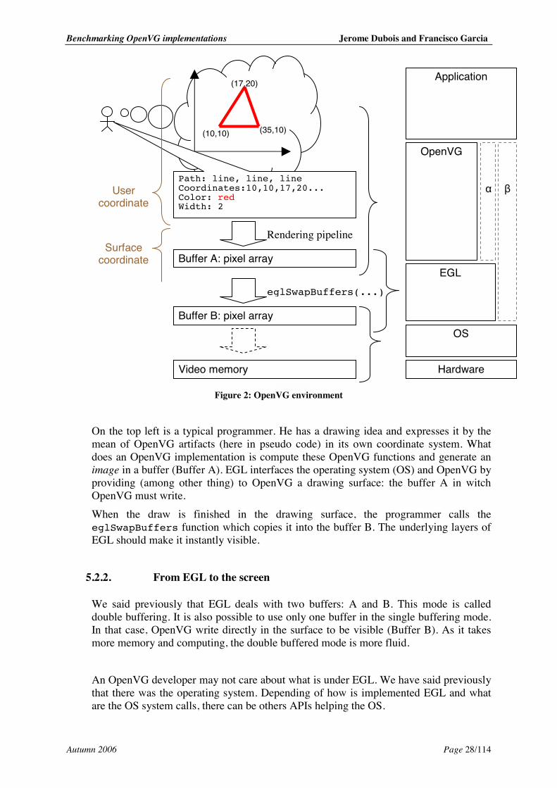
5.2.1. Layer organization of an OpenVG framework
OpenVG is system and hardware independent. This is a huge quality, but this also means that there is a set of others layers system dependant underlying it. Just under OpenVG is an API called EGL, released by Khronos as well. We present here a scheme representing the OpenVG and EGL environment and how they interact. On the right is the layered organization of the platform and on the left is an outline of what is done at each stage.
Benchmarking OpenVG implementations Jerome Dubois and Francisco Garcia
Autumn 2006 Page 28/114
Figure 2: OpenVG environment
On the top left is a typical programmer. He has a drawing idea and expresses it by the mean of OpenVG artifacts (here in pseudo code) in its own coordinate system. What does an OpenVG implementation is compute these OpenVG functions and generate an image in a buffer (Buffer A). EGL interfaces the operating system (OS) and OpenVG by providing (among other thing) to OpenVG a drawing surface: the buffer A in witch OpenVG must write. When the draw is finished in the drawing surface, the programmer calls the eglSwapBuffers function which copies it into the buffer B. The underlying layers of EGL should make it instantly visible.
5.2.2. From EGL to the screen
We said previously that EGL deals with two buffers: A and B. This mode is called double buffering. It is also possible to use only one buffer in the single buffering mode. In that case, OpenVG write directly in the surface to be visible (Buffer B). As it takes more memory and computing, the double buffered mode is more fluid. An OpenVG developer may not care about what is under EGL. We have said previously that there was the operating system. Depending of how is implemented EGL and what are the OS system calls, there can be others APIs helping the OS.
(10,10)
(17,20)
(35,10)
Path: line, line, line Coordinates:10,10,17,20... Color: red Width: 2
Buffer A: pixel array
Buffer B: pixel array
Video memory
Hardware
OS
EGL
OpenVG
Application
User
coordinates
Surface coordinate
s
Rendering pipeline
eglSwapBuffers(...)
Benchmarking OpenVG implementations Jerome Dubois and Francisco Garcia
Autumn 2006 Page 29/114
Most of the time, EGL implementations use the C API called GLUT (OpenGL Utility Toolkit). This API is widely used by OpenGL developers. According to its author, it has two purposes [B6]: “provides a way to write OpenGL programs without the complexity entailed by the details of the native window system APIs […], demonstrate proper handling of a variety of OpenGL and X integration issues”. Most EGL implementations rely or require the use of GLUT. It provides to EGL a system window and deals with events and time [B7]. The user application can use it as a scheduler: every time an event arrives (a key has been pressed on the keyboard, the window has been resized, a timer has ended…), GLUT calls the appropriate OpenVG code to possibly redraw an image. Inside the OS is a complicate structure, and we should relativize the instantaneous apparition on the screen of the buffer B. Indeed, the window manager and graphic environments (X Window, explorer.exe, KDE, Gnome…) can store the image somewhere in memory and really make it visible when the window is maximized. On the other hand, on an embedded device, the buffer B in which EGL or OpenVG writes may be directly the video memory, if the graphic interface is programmed over OpenVG for example. The nice thing about OpenVG is that the application developers do not need to be aware of the EGL underlying architecture.
5.2.3. OpenVG collaborating with others APIs
• OpenGL ES or other graphical API
OpenVG is a 2D vector graphic API. Maybe the programmer needs some raster graphic tools; maybe he wants to use another graphical API! It is possible by different means.
On the Figure 2, we have drawn a rectangular called representing a possible other API, most of the time OpenGL ES (2D-3D raster graphic API).
These APIs can interact together by three ways, maybe more:
! Both APIs use the same rendering surface (Buffer B) ! The OpenVG rendering surface is a buffer in memory used by OpenGL ES as an
image, a texture… ! OpenGL ES writes in a buffer (its rendering surface) used by OpenVG as an
image, a tilling pattern…
• Non graphical APIs
To make our layered description complete, we have drawn a rectangle called on the Figure 2. This includes many tools which can deal with sound, advanced mathematic functions, network, time and so forth. The graphical aspect of the application is maybe only a small part (though important!).
A part of GLUT is here as well.
5.2.4. EGL provides a drawing context
Benchmarking OpenVG implementations Jerome Dubois and Francisco Garcia
Autumn 2006 Page 30/114
Providing a drawing surface – a buffer to draw on – is not the only service given by EGL to OpenVG. It also created the drawing context in witch OpenVG works, and binds it to an execution flow (thread) in witch OpenVG functions run. Associated with a context is a set of fields representing the state of OpenVG execution. For example, the drawing context state describes the transformation to apply on images, the color used to clear the screen, or the latest unreported error code (equivalent of the C errno). It may be possible not to use EGL even if it has strongly been thought to be used. In that case, the host framework must provide some similar services.
At this point of the document, it may be interesting for the reader to read the two Khronos web pages about OpenVG and EGL. This is neither so long nor complicated.
5.3. GENERAL NOTIONS
OpenVG is an API for C and C++ programming language. All its given types and function are defined or accessible using the header openvg.h. Implementations just have to provide a (dynamic) library to link with. For the use of EGL, the header egl.h is included. Most of the quoted C definitions below are from openvg.h, and the application code is from us.
OpenVG specifications define a set of types used everywhere in a code using OpenVG API: typedef float VGfloat; typedef signed char VGbyte; typedef unsigned char VGubyte; typedef short VGshort; typedef int VGint; typedef unsigned int VGuint; typedef unsigned int VGbitfield; typedef enum { VG_FALSE = 0, VG_TRUE = 1 } VGboolean;
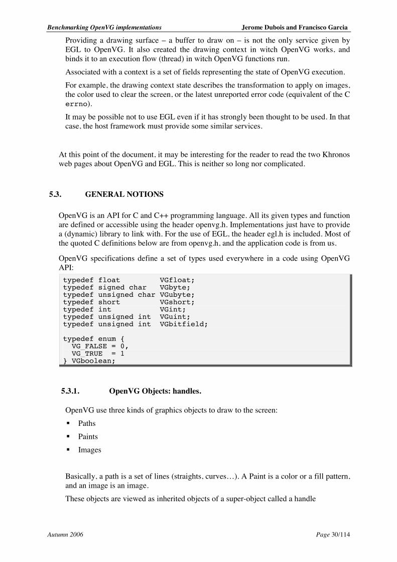
5.3.1. OpenVG Objects: handles.
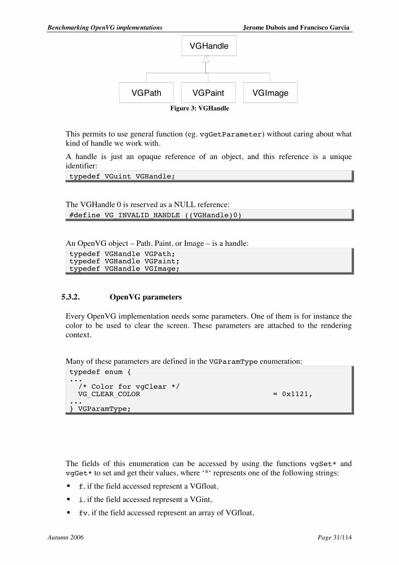
OpenVG use three kinds of graphics objects to draw to the screen: ! Paths ! Paints ! Images Basically, a path is a set of lines (straights, curves…). A Paint is a color or a fill pattern, and an image is an image. These objects are viewed as inherited objects of a super-object called a handle
Benchmarking OpenVG implementations Jerome Dubois and Francisco Garcia
Autumn 2006 Page 31/114
VGHandle
VGPaintVGPath VGImage
Figure 3: VGHandle
This permits to use general function (eg. vgGetParameter) without caring about what kind of handle we work with. A handle is just an opaque reference of an object, and this reference is a unique identifier: typedef VGuint VGHandle;
The VGHandle 0 is reserved as a NULL reference: #define VG_INVALID_HANDLE ((VGHandle)0)
An OpenVG object – Path, Paint, or Image – is a handle: typedef VGHandle VGPath; typedef VGHandle VGPaint; typedef VGHandle VGImage;
5.3.2. OpenVG parameters
Every OpenVG implementation needs some parameters. One of them is for instance the color to be used to clear the screen. These parameters are attached to the rendering context. Many of these parameters are defined in the VGParamType enumeration: typedef enum { ... /* Color for vgClear */ VG_CLEAR_COLOR = 0x1121, ... } VGParamType;
The fields of this enumeration can be accessed by using the functions vgSet* and vgGet* to set and get their values, where ‘*‘ represents one of the following strings: ! f, if the field accessed represent a VGfloat, ! i, if the field accessed represent a VGint, ! fv, if the field accessed represent an array of VGfloat,
Benchmarking OpenVG implementations Jerome Dubois and Francisco Garcia
Autumn 2006 Page 32/114
! iv, if the field accessed represent an array of VGint. For changing the color used to clean the surface, the code will be: VGfloat clearColor [4]={0.5, 0.5, 1, 0.8}; vgSetfv(VG_CLEAR_COLOR, 4, clearColor);
5.3.3. Handle parameters
With the same idea of OpenVG parameters, each created handle has a set of parameters attached. They are defined in one of the three enumerations ! VGPathParamType ! VGPaintParamType ! VGImageParamType They can be accessed by the functions vgSetParameter* and vgGetParameter*, where ‘*‘ is ‘f’, ‘i’, “fv” or “iv” with the same meaning as for OpenVG parameters in previous section (5.3.2). Some of the handle parameters are vectors of undefined size. The function vgGetParameterVectorSize permits to know the size of the actual vector value.
5.3.4. Coordinate systems and transformations
As seen in Figure 2 page 28, we use different coordinate systems: ! User (Path)
The user expresses the paths coordinates in its own coordinate system.
! User (Images) The user expresses the images coordinates in a particular coordinate system.
! Paint The user express the Paint coordinates in a particular coordinate system.
! Surface These are the coordinates in the rendering surface. They are screen or window dependant.
During the stage 6 of the rendering pipeline, the Paint coordinates are transformed into surface-coordinates using a combination of the transformations called Paint-to-user and Path-user-to-surface. During the stage 7 of the rendering pipeline, the user Image coordinates are transformed into surface-coordinates using a transformation called Image-user-to-surface. During the stage 3 of the rendering pipeline, the user Path coordinates are transformed into surface-coordinates using a transformation called Path-user-to-surface.
Benchmarking OpenVG implementations Jerome Dubois and Francisco Garcia
Autumn 2006 Page 33/114
5.3.5. All OpenVG parameters
In addition to the fields of the enumeration VGParamType (cf. 5.3.2), the parameters attached to the rendering context are: ! The drawing surface ! The 4 transformation matrixes (cf. 5.4.4) ! The oldest unreported error ! The Mask and the mask enable flag ! Paints (Stroking and filling Paints)
5.4. TRANSFORMATIONS
5.4.1. When do the transformations occur?
• User to surface transformations
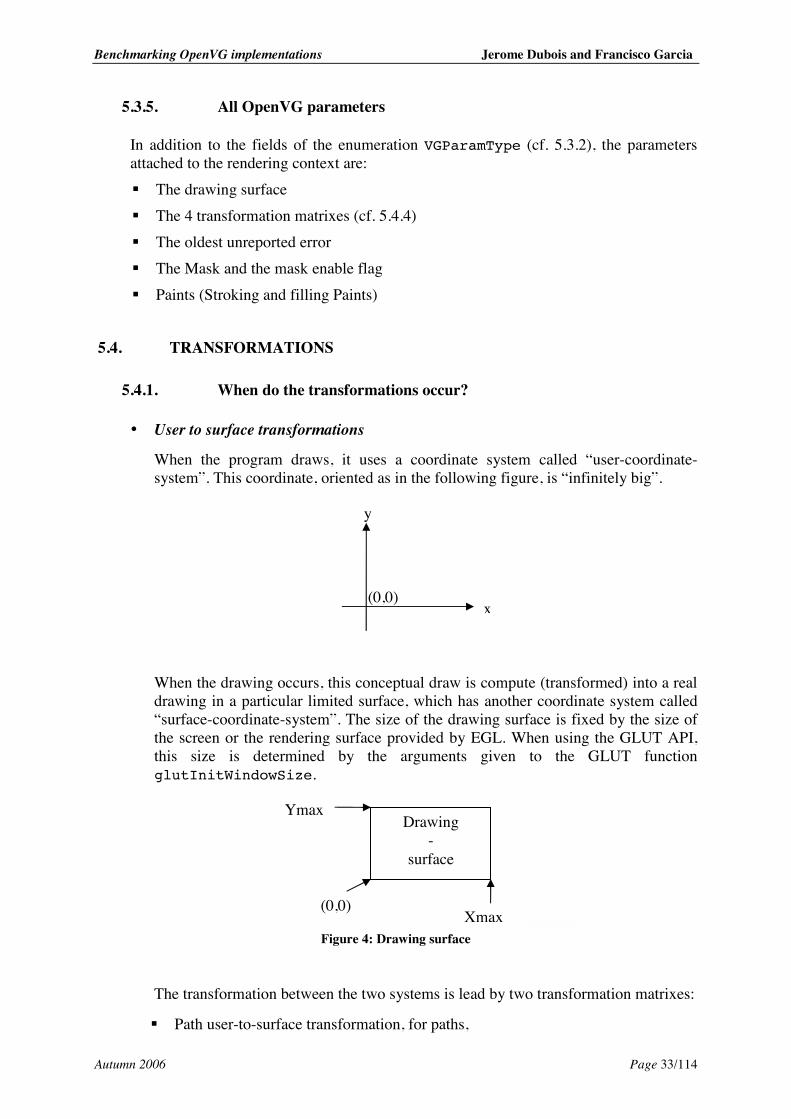
When the program draws, it uses a coordinate system called “user-coordinate-system”. This coordinate, oriented as in the following figure, is “infinitely big”.
When the drawing occurs, this conceptual draw is compute (transformed) into a real drawing in a particular limited surface, which has another coordinate system called “surface-coordinate-system”. The size of the drawing surface is fixed by the size of the screen or the rendering surface provided by EGL. When using the GLUT API, this size is determined by the arguments given to the GLUT function glutInitWindowSize.
Figure 4: Drawing surface
The transformation between the two systems is lead by two transformation matrixes:
! Path user-to-surface transformation, for paths,
x
y
(0,0)
Ymax
(0,0)
Drawing -
surface
Xmax
Benchmarking OpenVG implementations Jerome Dubois and Francisco Garcia
Autumn 2006 Page 34/114
! Paint user-to-surface transformation, for paints.
In this section (5.4), we will focus more on Path user-to-surface transformation, though it is similar for Paints.
The nice consequence of this mechanism is that the application is independent of the actual size of the screen. Thus, application developers can choose their own coordinate system, and simply use the right transformation so that it fits the actual screen. In a window environment where the size of the window can change, this can avoid lots of pitfalls.
• Paint to user transformations
When working on Paint (cf. 5.8), the programmer uses yet another coordinate system. The Paint coordinates are transformed to the user coordinates using the matrixes Fill-Paint-to-user and Stroke-Paint-to-user, depending whether the Paint is used to fill or stroke a Path.
5.4.2. Homogeneous coordinates and transformation matrixes
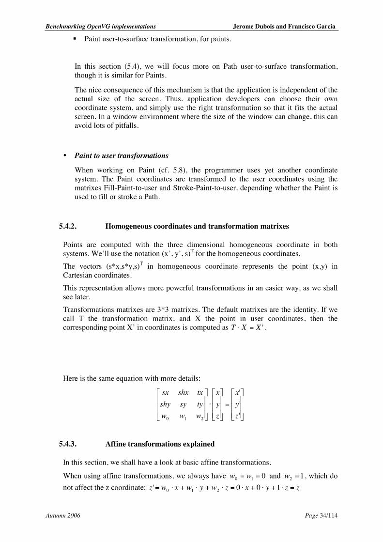
Points are computed with the three dimensional homogeneous coordinate in both systems. We’ll use the notation (x’, y’, s)T for the homogeneous coordinates. The vectors (s*x,s*y,s)T in homogeneous coordinate represents the point (x,y) in Cartesian coordinates. This representation allows more powerful transformations in an easier way, as we shall see later. Transformations matrixes are 3*3 matrixes. The default matrixes are the identity. If we call T the transformation matrix, and X the point in user coordinates, then the corresponding point X’ in coordinates is computed as 'XXT =⋅ . Here is the same equation with more details:
=
⋅
'''
210 zyx
zyx
wwwtysyshytxshxsx
5.4.3. Affine transformations explained
In this section, we shall have a look at basic affine transformations.
When using affine transformations, we always have 010 == ww and 12 =w , which do not affect the z coordinate: zzyxzwywxwz =⋅+⋅+⋅=⋅+⋅+⋅= 100' 210
Benchmarking OpenVG implementations Jerome Dubois and Francisco Garcia
Autumn 2006 Page 35/114
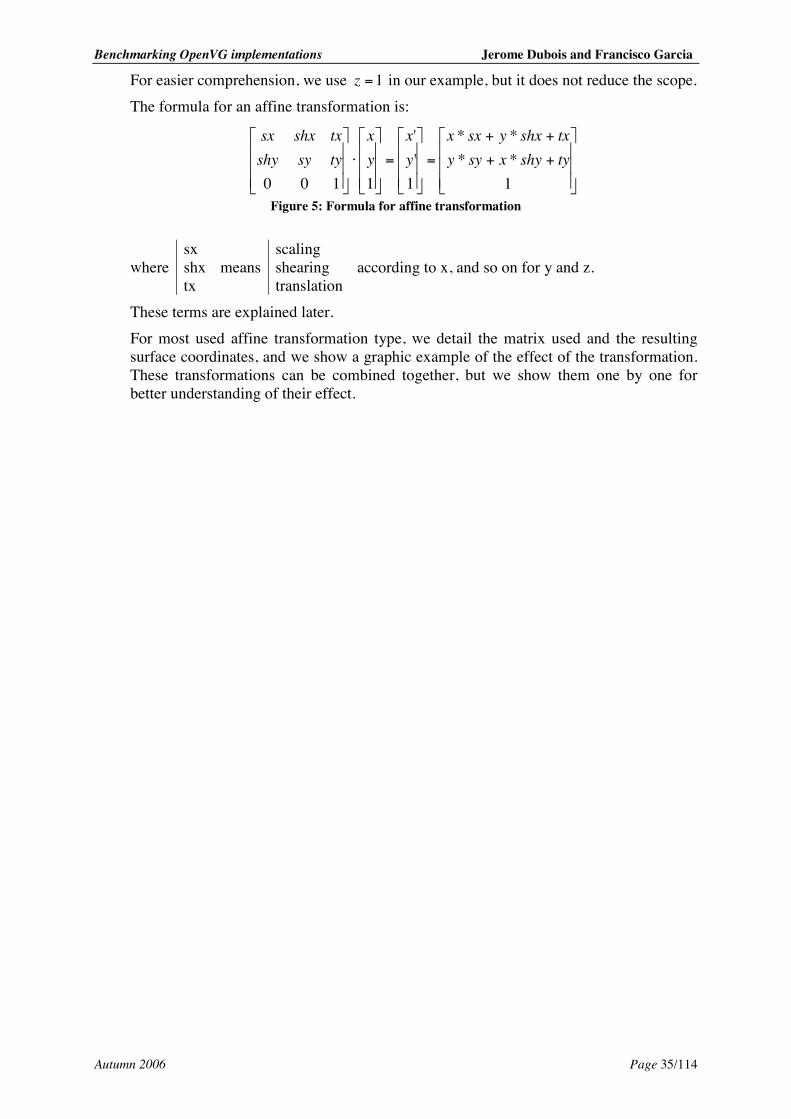
For easier comprehension, we use 1=z in our example, but it does not reduce the scope. The formula for an affine transformation is:
++
++
=
=
⋅
1****
1''
1100tyshyxsyytxshxysxx
yx
yx
tysyshytxshxsx
Figure 5: Formula for affine transformation
where sx shx tx
means scaling shearing translation
according to x, and so on for y and z.
These terms are explained later. For most used affine transformation type, we detail the matrix used and the resulting surface coordinates, and we show a graphic example of the effect of the transformation. These transformations can be combined together, but we show them one by one for better understanding of their effect.
Benchmarking OpenVG implementations Jerome Dubois and Francisco Garcia
Autumn 2006 Page 36/114
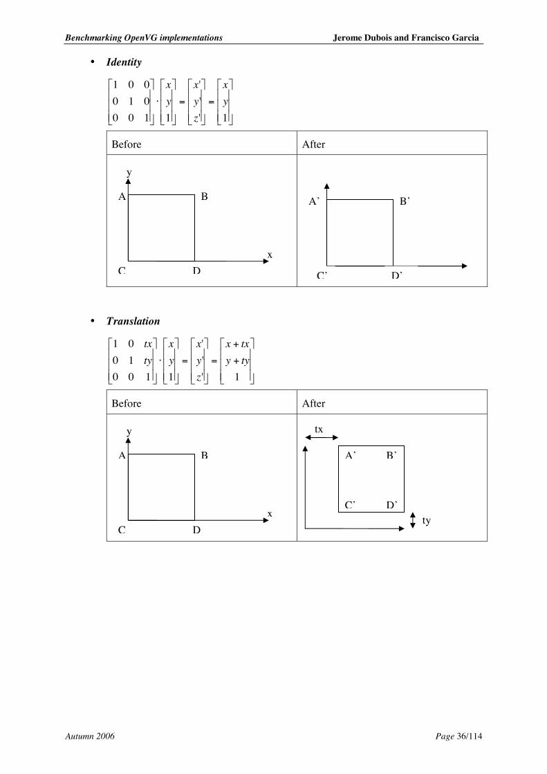
• Identity
=
=
⋅
1'''
1100010001
yx
zyx
yx
Before After
• Translation
+
+
=
=
⋅
1'''
11001001
tyytxx
zyx
yx
tytx
Before After
B’ A’
C’ D’
tx
ty
y
Dx
B A
C
y
Dx
B A
C
B’ A’
C’ D’
Benchmarking OpenVG implementations Jerome Dubois and Francisco Garcia
Autumn 2006 Page 37/114
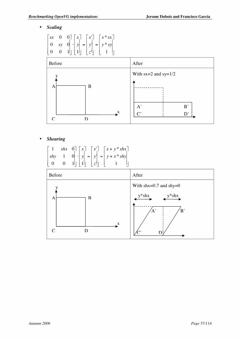
• Scaling
=
=
⋅
1**
'''
11000000
syysxx
zyx
yx
sysx
Before After
With sx=2 and sy=1/2
• Shearing
+
+
=
=
⋅
1**
'''
11000101
shyxyshxyx
zyx
yx
shyshx
Before After
With shx=0.7 and shy=0
y
Dx
B A
C
y
Dx
B A
C
B’ A’ C’ D’
C’
A’
D’
B’
y*shx y*shx
Benchmarking OpenVG implementations Jerome Dubois and Francisco Garcia
Autumn 2006 Page 38/114
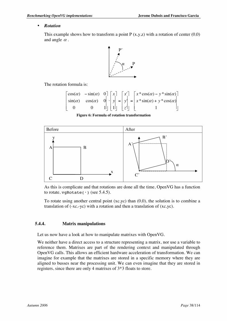
• Rotation
This example shows how to transform a point P (x,y,z) with a rotation of center (0,0) and angle α .
The rotation formula is:
+
−
=
=
⋅
−
1)cos(*)sin(*)sin(*)cos(*
'''
11000)cos()sin(0)sin()cos(
αα
αα
αα
αα
yxyx
zyx
yx
Figure 6: Formula of rotation transformation
Before After
As this is complicate and that rotations are done all the time, OpenVG has a function to rotate, vgRotate(•) (see 5.4.5).
To rotate using another central point (xc,yc) than (0,0), the solution is to combine a translation of (-xc,-yc) with a rotation and then a translation of (xc,yc).
5.4.4. Matrix manipulations
Let us now have a look at how to manipulate matrixes with OpenVG. We neither have a direct access to a structure representing a matrix, nor use a variable to reference them. Matrixes are part of the rendering context and manipulated through OpenVG calls. This allows an efficient hardware acceleration of transformation. We can imagine for example that the matrixes are stored in a specific memory where they are aligned to busses near the processing unit. We can even imagine that they are stored in registers, since there are only 4 matrixes of 3*3 floats to store.
P’
P
y
Dx
B A
C
D’
B’ A’
C’
Benchmarking OpenVG implementations Jerome Dubois and Francisco Garcia
Autumn 2006 Page 39/114
Four matrixes we said? Yes, and we can refer to them with this enumeration: typedef enum { VG_MATRIX_PATH_USER_TO_SURFACE = 0x1400, VG_MATRIX_IMAGE_USER_TO_SURFACE = 0x1401, VG_MATRIX_FILL_PAINT_TO_USER = 0x1402, VG_MATRIX_STROKE_PAINT_TO_USER = 0x1403 } VGMatrixMode;
Where: ! VG_MATRIX_PATH_USER_TO_SURFACE refers the matrix used on Path when
transforming them from user coordinates to surface coordinates; ! VG_MATRIX_IMAGE_USER_TO_SURFACE refers the matrix used on Images when
transforming them from user coordinates to surface coordinates; ! VG_MATRIX_FILL_PAINT_TO_USER refers the matrix used on Paints used for
filling Paths, when transforming them from Paint user coordinates to user coordinates;
! VG_MATRIX_STROKE_PAINT_TO_USER refers the matrix used on Paints used for stroking Paths, when transforming them from Paint user coordinates to user coordinates.
• Set a current matrix
We use these constants to define a “current matrix”, and all matrix manipulation functions work implicitly on the current matrix.
For setting VG_MATRIX_IMAGE_USER_TO_SURFACE as the current matrix for example, the code is: vgSeti(VG_MATRIX_MODE, VG_MATRIX_IMAGE_USER_TO_SURFACE) ;
• Manipulate the current matrix
We present here some of OpenVG functions to manipulate the current matrix.
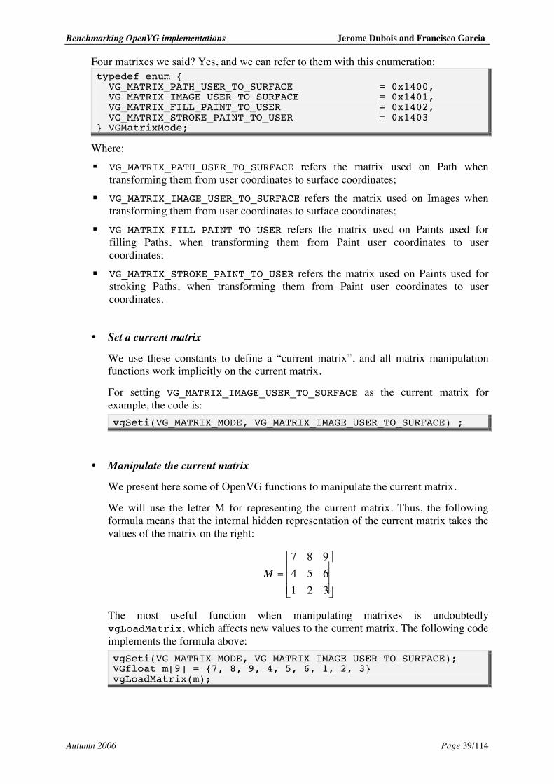
We will use the letter M for representing the current matrix. Thus, the following formula means that the internal hidden representation of the current matrix takes the values of the matrix on the right:
=
321654987
M
The most useful function when manipulating matrixes is undoubtedly vgLoadMatrix, which affects new values to the current matrix. The following code implements the formula above: vgSeti(VG_MATRIX_MODE, VG_MATRIX_IMAGE_USER_TO_SURFACE); VGfloat m[9] = {7, 8, 9, 4, 5, 6, 1, 2, 3} vgLoadMatrix(m);
Benchmarking OpenVG implementations Jerome Dubois and Francisco Garcia
Autumn 2006 Page 40/114
Another function is vgGetMatrix, which is useful to know the values of the current matrix: vgGetMatrix(m);
The last function we will detail permits to multiply the current matrix by another, in order to combine the old transformation with a new one:
⋅=
1006.8527.0
420
oldnew MM
The corresponding code is: VGfloat m[9] = {0, 2, 4, 0.27, 5, 8.6, 0, 0, 1} vgMultMatrix(m);
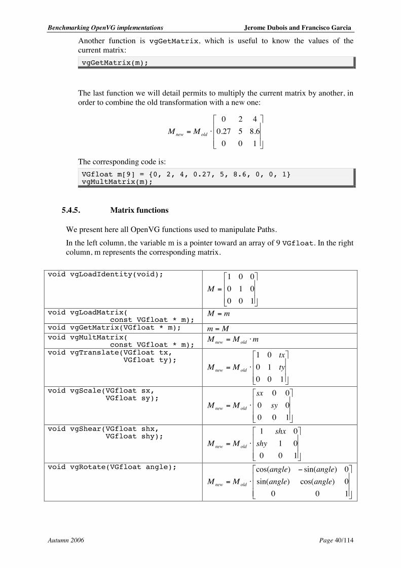
5.4.5. Matrix functions
We present here all OpenVG functions used to manipulate Paths. In the left column, the variable m is a pointer toward an array of 9 VGfloat. In the right column, m represents the corresponding matrix.
void vgLoadIdentity(void);
=
100010001
M
void vgLoadMatrix( const VGfloat * m);
mM =
void vgGetMatrix(VGfloat * m); Mm = void vgMultMatrix( const VGfloat * m);
mMM oldnew ⋅= void vgTranslate(VGfloat tx, VGfloat ty);
⋅=
1001001
tytx
MM oldnew
void vgScale(VGfloat sx, VGfloat sy);
⋅=
1000000
sysx
MM oldnew
void vgShear(VGfloat shx, VGfloat shy);
⋅=
1000101
shyshx
MM oldnew
void vgRotate(VGfloat angle);
−
⋅=
1000)cos()sin(0)sin()cos(
angleangleangleangle
MM oldnew
Benchmarking OpenVG implementations Jerome Dubois and Francisco Garcia
Autumn 2006 Page 41/114
5.4.6. Benefit of hardware accelerated transformation
The functions presented in the previous section are supposed to be hardware accelerated. It is thus a good idea for the programmer to use them, rather than computing matrixes directly in C or with other software tools. Let us explain in a simple example how they can be useful. As we explained earlier, if we want to rotate a draw with center C (cx,cy) and angle , we have to: ! translate with vector (-cx,-cy), ! rotate with angle , ! translate with vector (cx,cy). Let us call Ti, Rii, and Tiii the three corresponding transformation matrixes. A good idea is to wonder if we know statically the center and the angle of the rotation. If the answer is yes, we should compute them statically: TiRiiTiiiN ⋅⋅= and use vgLoadMatrix(N) (informal notation), with the values of N written in the code. If we don’t know these values statically, we cannot proceed like that. This case can happen in a game when the programmer wants to rotate a draw according to the action of the player for instance. In that case, we have two solutions: ! compute outside OpenVG:
TiRiiTiiiN ⋅⋅= /* informal notation */ vgMultMatrix(N)
! compute inside OpenVG vgMultMatrix(Ti ) vgMultMatrix(Rii ) vgMultMatrix(Tiii)
In the first solution, the computation of the three matrixes is done by software tools. In the second, it is done by OpenVG API, probably hardware accelerated.
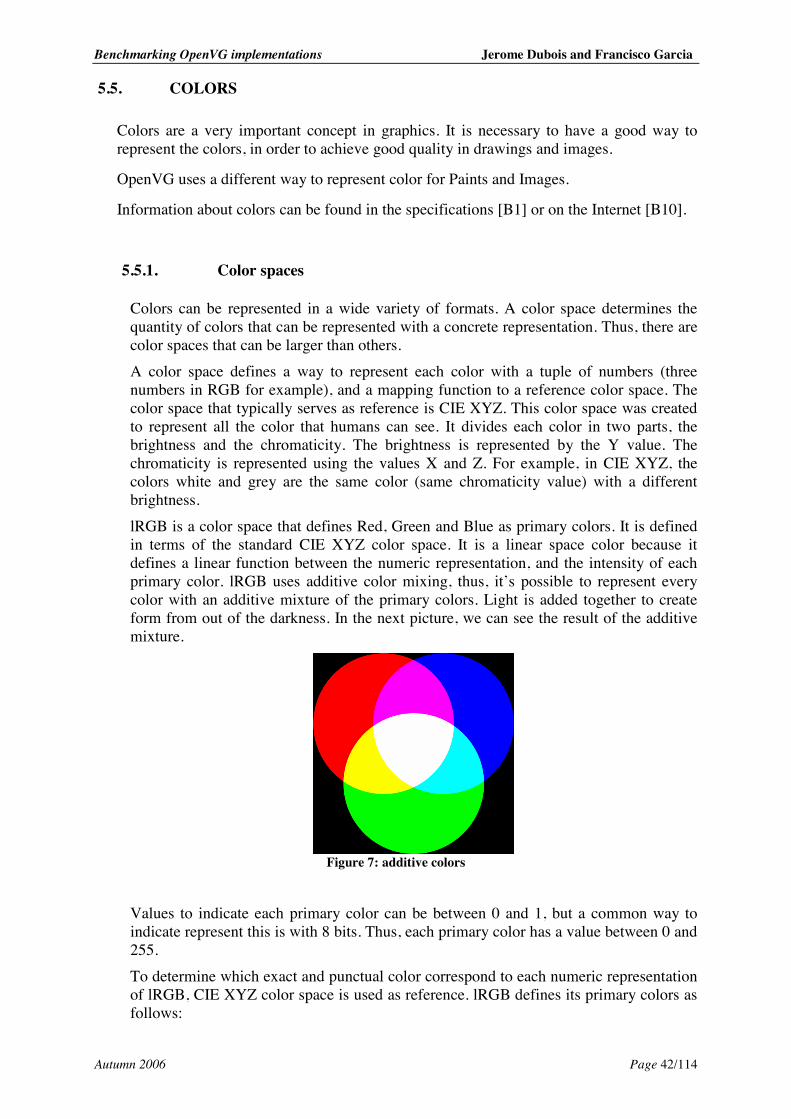
Benchmarking OpenVG implementations Jerome Dubois and Francisco Garcia
Autumn 2006 Page 42/114
5.5. COLORS
Colors are a very important concept in graphics. It is necessary to have a good way to represent the colors, in order to achieve good quality in drawings and images.
OpenVG uses a different way to represent color for Paints and Images.
Information about colors can be found in the specifications [B1] or on the Internet [B10].
5.5.1. Color spaces
Colors can be represented in a wide variety of formats. A color space determines the quantity of colors that can be represented with a concrete representation. Thus, there are color spaces that can be larger than others. A color space defines a way to represent each color with a tuple of numbers (three numbers in RGB for example), and a mapping function to a reference color space. The color space that typically serves as reference is CIE XYZ. This color space was created to represent all the color that humans can see. It divides each color in two parts, the brightness and the chromaticity. The brightness is represented by the Y value. The chromaticity is represented using the values X and Z. For example, in CIE XYZ, the colors white and grey are the same color (same chromaticity value) with a different brightness. lRGB is a color space that defines Red, Green and Blue as primary colors. It is defined in terms of the standard CIE XYZ color space. It is a linear space color because it defines a linear function between the numeric representation, and the intensity of each primary color. lRGB uses additive color mixing, thus, it’s possible to represent every color with an additive mixture of the primary colors. Light is added together to create form from out of the darkness. In the next picture, we can see the result of the additive mixture.
Figure 7: additive colors
Values to indicate each primary color can be between 0 and 1, but a common way to indicate represent this is with 8 bits. Thus, each primary color has a value between 0 and 255. To determine which exact and punctual color correspond to each numeric representation of lRGB, CIE XYZ color space is used as reference. lRGB defines its primary colors as follows:
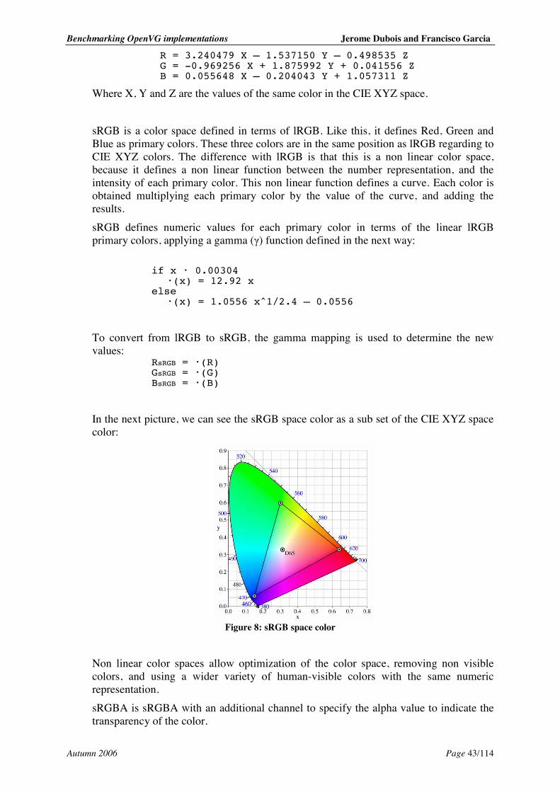
Benchmarking OpenVG implementations Jerome Dubois and Francisco Garcia
Autumn 2006 Page 43/114
R = 3.240479 X – 1.537150 Y – 0.498535 Z G = -0.969256 X + 1.875992 Y + 0.041556 Z B = 0.055648 X – 0.204043 Y + 1.057311 Z
Where X, Y and Z are the values of the same color in the CIE XYZ space. sRGB is a color space defined in terms of lRGB. Like this, it defines Red, Green and Blue as primary colors. These three colors are in the same position as lRGB regarding to CIE XYZ colors. The difference with lRGB is that this is a non linear color space, because it defines a non linear function between the number representation, and the intensity of each primary color. This non linear function defines a curve. Each color is obtained multiplying each primary color by the value of the curve, and adding the results. sRGB defines numeric values for each primary color in terms of the linear lRGB primary colors, applying a gamma () function defined in the next way:
if x • 0.00304 •(x) = 12.92 x else •(x) = 1.0556 x^1/2.4 – 0.0556
To convert from lRGB to sRGB, the gamma mapping is used to determine the new values:
RsRGB = •(R) GsRGB = •(G) BsRGB = •(B)
In the next picture, we can see the sRGB space color as a sub set of the CIE XYZ space color:
Figure 8: sRGB space color
Non linear color spaces allow optimization of the color space, removing non visible colors, and using a wider variety of human-visible colors with the same numeric representation. sRGBA is sRGBA with an additional channel to specify the alpha value to indicate the transparency of the color.
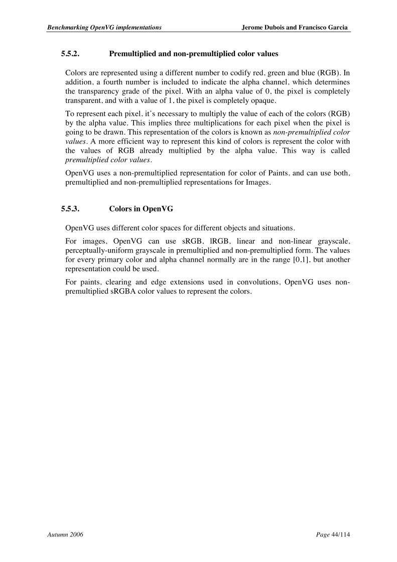
Benchmarking OpenVG implementations Jerome Dubois and Francisco Garcia
Autumn 2006 Page 44/114
5.5.2. Premultiplied and non-premultiplied color values
Colors are represented using a different number to codify red, green and blue (RGB). In addition, a fourth number is included to indicate the alpha channel, which determines the transparency grade of the pixel. With an alpha value of 0, the pixel is completely transparent, and with a value of 1, the pixel is completely opaque. To represent each pixel, it’s necessary to multiply the value of each of the colors (RGB) by the alpha value. This implies three multiplications for each pixel when the pixel is going to be drawn. This representation of the colors is known as non-premultiplied color values. A more efficient way to represent this kind of colors is represent the color with the values of RGB already multiplied by the alpha value. This way is called premultiplied color values. OpenVG uses a non-premultiplied representation for color of Paints, and can use both, premultiplied and non-premultiplied representations for Images.
5.5.3. Colors in OpenVG
OpenVG uses different color spaces for different objects and situations. For images, OpenVG can use sRGB, lRGB, linear and non-linear grayscale, perceptually-uniform grayscale in premultiplied and non-premultiplied form. The values for every primary color and alpha channel normally are in the range [0,1], but another representation could be used. For paints, clearing and edge extensions used in convolutions, OpenVG uses non-premultiplied sRGBA color values to represent the colors.
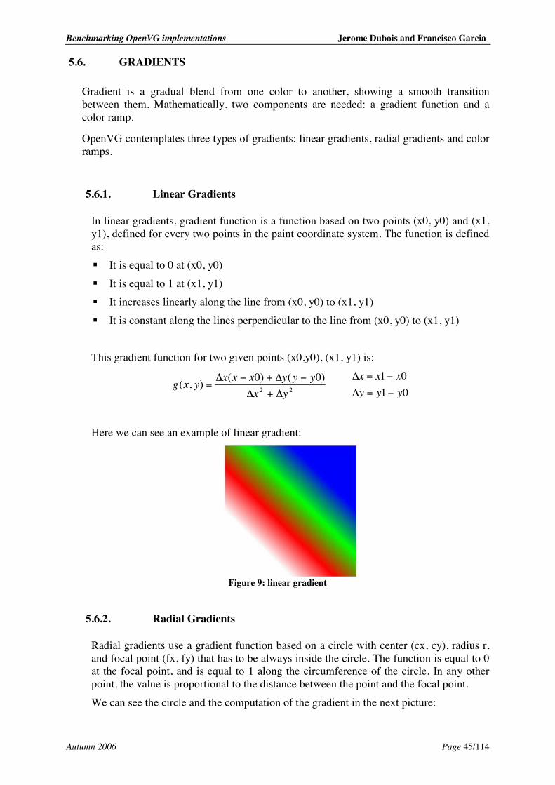
Benchmarking OpenVG implementations Jerome Dubois and Francisco Garcia
Autumn 2006 Page 45/114
5.6. GRADIENTS
Gradient is a gradual blend from one color to another, showing a smooth transition between them. Mathematically, two components are needed: a gradient function and a color ramp.
OpenVG contemplates three types of gradients: linear gradients, radial gradients and color ramps.
5.6.1. Linear Gradients
In linear gradients, gradient function is a function based on two points (x0, y0) and (x1, y1), defined for every two points in the paint coordinate system. The function is defined as: ! It is equal to 0 at (x0, y0) ! It is equal to 1 at (x1, y1) ! It increases linearly along the line from (x0, y0) to (x1, y1) ! It is constant along the lines perpendicular to the line from (x0, y0) to (x1, y1) This gradient function for two given points (x0,y0), (x1, y1) is:
22
)0()0(),(yx
yyyxxxyxgΔ+Δ
−Δ+−Δ=
0101
yyyxxx
−=Δ
−=Δ
Here we can see an example of linear gradient:
Figure 9: linear gradient
5.6.2. Radial Gradients
Radial gradients use a gradient function based on a circle with center (cx, cy), radius r, and focal point (fx, fy) that has to be always inside the circle. The function is equal to 0 at the focal point, and is equal to 1 along the circumference of the circle. In any other point, the value is proportional to the distance between the point and the focal point. We can see the circle and the computation of the gradient in the next picture:
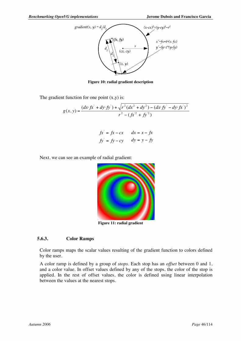
Benchmarking OpenVG implementations Jerome Dubois and Francisco Garcia
Autumn 2006 Page 46/114
Figure 10: radial gradient description
The gradient function for one point (x,y) is:
)()··()()··(
),( 2'2'2
2''222''
fyfxrfxdyfydxdydxrfydyfxdx
yxg+−
−−+++=
cyfyfycxfxfx
−=
−='
'
fyydyfxxdx
−=
−=
Next, we can see an example of radial gradient:
Figure 11: radial gradient
5.6.3. Color Ramps
Color ramps maps the scalar values resulting of the gradient function to colors defined by the user. A color ramp is defined by a group of stops. Each stop has an offset between 0 and 1, and a color value. In offset values defined by any of the stops, the color of the stop is applied. In the rest of offset values, the color is defined using linear interpolation between the values at the nearest stops.
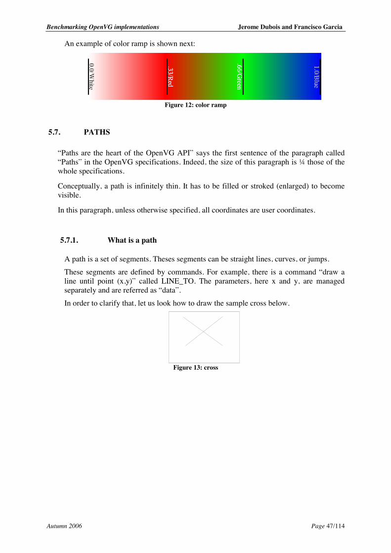
Benchmarking OpenVG implementations Jerome Dubois and Francisco Garcia
Autumn 2006 Page 47/114
An example of color ramp is shown next:
Figure 12: color ramp
5.7. PATHS
“Paths are the heart of the OpenVG API” says the first sentence of the paragraph called “Paths” in the OpenVG specifications. Indeed, the size of this paragraph is ¼ those of the whole specifications.
Conceptually, a path is infinitely thin. It has to be filled or stroked (enlarged) to become visible.
In this paragraph, unless otherwise specified, all coordinates are user coordinates.
5.7.1. What is a path
A path is a set of segments. Theses segments can be straight lines, curves, or jumps. These segments are defined by commands. For example, there is a command “draw a line until point (x,y)” called LINE_TO. The parameters, here x and y, are managed separately and are referred as “data”. In order to clarify that, let us look how to draw the sample cross below.
Figure 13: cross
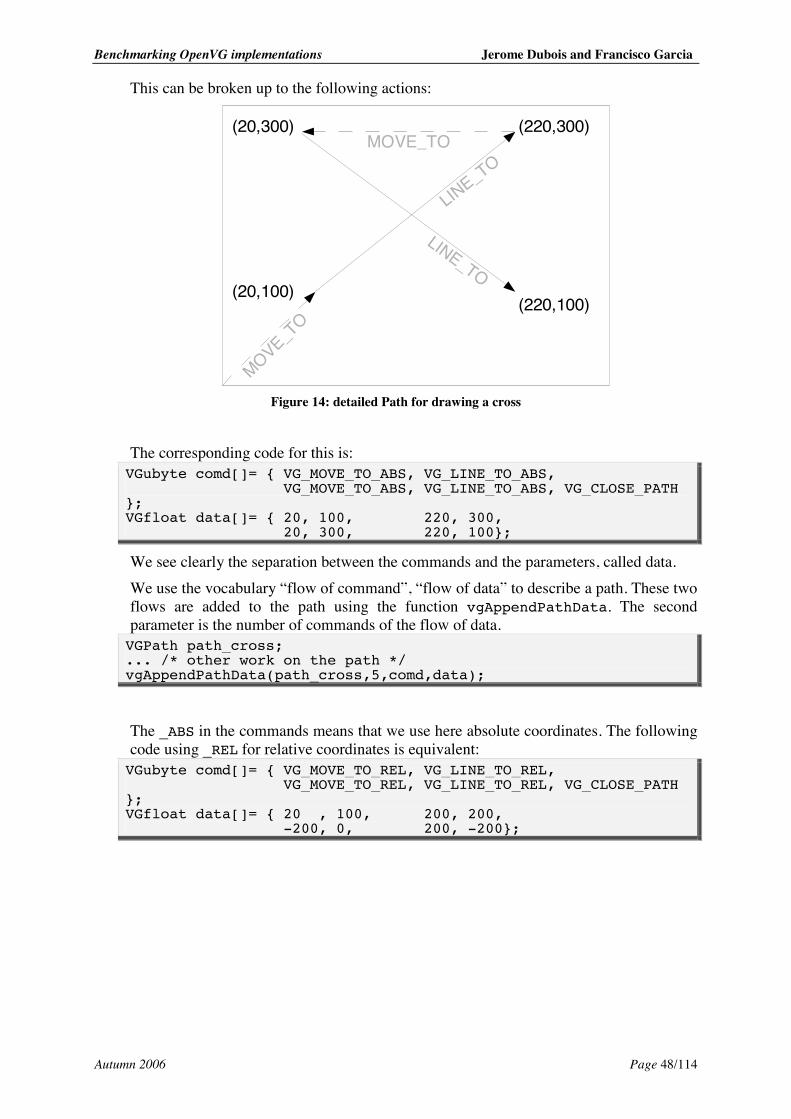
Benchmarking OpenVG implementations Jerome Dubois and Francisco Garcia
Autumn 2006 Page 48/114
This can be broken up to the following actions:
MOVE_TO
LINE_TO
MOVE_TO LINE_TO
(20,100)
(20,300) (220,300)
(220,100)
Figure 14: detailed Path for drawing a cross
The corresponding code for this is: VGubyte comd[]= { VG_MOVE_TO_ABS, VG_LINE_TO_ABS, VG_MOVE_TO_ABS, VG_LINE_TO_ABS, VG_CLOSE_PATH }; VGfloat data[]= { 20, 100, 220, 300, 20, 300, 220, 100};
We see clearly the separation between the commands and the parameters, called data. We use the vocabulary “flow of command”, “flow of data” to describe a path. These two flows are added to the path using the function vgAppendPathData. The second parameter is the number of commands of the flow of data. VGPath path_cross; ... /* other work on the path */ vgAppendPathData(path_cross,5,comd,data);
The _ABS in the commands means that we use here absolute coordinates. The following code using _REL for relative coordinates is equivalent: VGubyte comd[]= { VG_MOVE_TO_REL, VG_LINE_TO_REL, VG_MOVE_TO_REL, VG_LINE_TO_REL, VG_CLOSE_PATH }; VGfloat data[]= { 20 , 100, 200, 200, -200, 0, 200, -200};
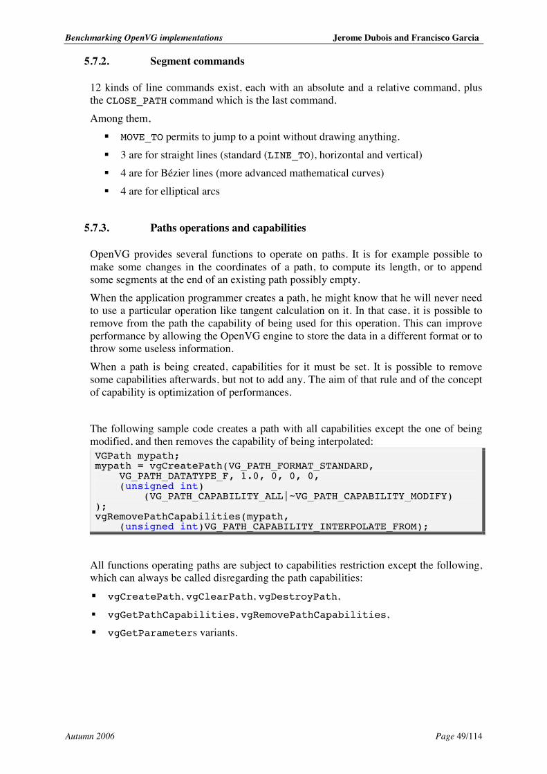
Benchmarking OpenVG implementations Jerome Dubois and Francisco Garcia
Autumn 2006 Page 49/114
5.7.2. Segment commands
12 kinds of line commands exist, each with an absolute and a relative command, plus the CLOSE_PATH command which is the last command. Among them,
! MOVE_TO permits to jump to a point without drawing anything. ! 3 are for straight lines (standard (LINE_TO), horizontal and vertical) ! 4 are for Bézier lines (more advanced mathematical curves) ! 4 are for elliptical arcs
5.7.3. Paths operations and capabilities
OpenVG provides several functions to operate on paths. It is for example possible to make some changes in the coordinates of a path, to compute its length, or to append some segments at the end of an existing path possibly empty. When the application programmer creates a path, he might know that he will never need to use a particular operation like tangent calculation on it. In that case, it is possible to remove from the path the capability of being used for this operation. This can improve performance by allowing the OpenVG engine to store the data in a different format or to throw some useless information. When a path is being created, capabilities for it must be set. It is possible to remove some capabilities afterwards, but not to add any. The aim of that rule and of the concept of capability is optimization of performances. The following sample code creates a path with all capabilities except the one of being modified, and then removes the capability of being interpolated: VGPath mypath; mypath = vgCreatePath(VG_PATH_FORMAT_STANDARD, VG_PATH_DATATYPE_F, 1.0, 0, 0, 0, (unsigned int) (VG_PATH_CAPABILITY_ALL|~VG_PATH_CAPABILITY_MODIFY) ); vgRemovePathCapabilities(mypath, (unsigned int)VG_PATH_CAPABILITY_INTERPOLATE_FROM);
All functions operating paths are subject to capabilities restriction except the following, which can always be called disregarding the path capabilities: ! vgCreatePath, vgClearPath, vgDestroyPath, ! vgGetPathCapabilities, vgRemovePathCapabilities, ! vgGetParameters variants.
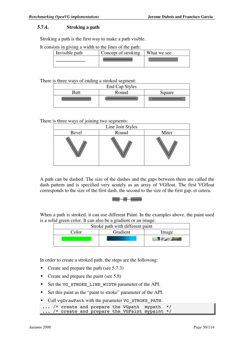
Benchmarking OpenVG implementations Jerome Dubois and Francisco Garcia
Autumn 2006 Page 50/114
5.7.4. Stroking a path
Stroking a path is the first way to make a path visible. It consists in giving a width to the lines of the path:
Invisible path Concept of stroking What we see
There is three ways of ending a stroked segment:
End Cap Styles Butt Round Square
There is three ways of joining two segments:
Line Join Styles Bevel Round Miter
A path can be dashed. The size of the dashes and the gaps between them are called the dash pattern and is specified very acutely as an array of VGfloat. The first VGfloat corresponds to the size of the first dash, the second to the size of the first gap, et cetera.
When a path is stroked, it can use different Paint. In the examples above, the paint used is a solid green color. It can also be a gradient or an image:
Stroke path with different paint Color Gradient Image
In order to create a stroked path, the steps are the following: ! Create and prepare the path (see 5.7.3) ! Create and prepare the paint (see 5.8) ! Set the VG_STROKE_LINE_WIDTH parameter of the API. ! Set this paint as the “paint to stroke” parameter of the API. ! Call vgDrawPath with the parameter VG_STROKE_PATH. ... /* create and prepare the VGpath mypath */ ... /* create and prepare the VGPaint mypaint */
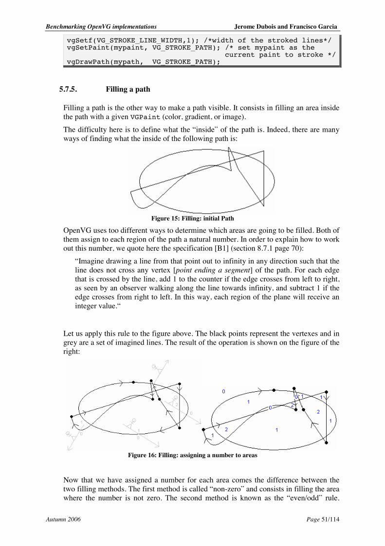
Benchmarking OpenVG implementations Jerome Dubois and Francisco Garcia
Autumn 2006 Page 51/114
vgSetf(VG_STROKE_LINE_WIDTH,1); /*width of the stroked lines*/ vgSetPaint(mypaint, VG_STROKE_PATH); /* set mypaint as the current paint to stroke */ vgDrawPath(mypath, VG_STROKE_PATH);
5.7.5. Filling a path
Filling a path is the other way to make a path visible. It consists in filling an area inside the path with a given VGPaint (color, gradient, or image). The difficulty here is to define what the “inside” of the path is. Indeed, there are many ways of finding what the inside of the following path is:
Figure 15: Filling: initial Path
OpenVG uses too different ways to determine which areas are going to be filled. Both of them assign to each region of the path a natural number. In order to explain how to work out this number, we quote here the specification [B1] (section 8.7.1 page 70):
“Imagine drawing a line from that point out to infinity in any direction such that the line does not cross any vertex [point ending a segment] of the path. For each edge that is crossed by the line, add 1 to the counter if the edge crosses from left to right, as seen by an observer walking along the line towards infinity, and subtract 1 if the edge crosses from right to left. In this way, each region of the plane will receive an integer value.“
Let us apply this rule to the figure above. The black points represent the vertexes and in grey are a set of imagined lines. The result of the operation is shown on the figure of the right:
Figure 16: Filling: assigning a number to areas
Now that we have assigned a number for each area comes the difference between the two filling methods. The first method is called “non-zero” and consists in filling the area where the number is not zero. The second method is known as the “even/odd” rule.
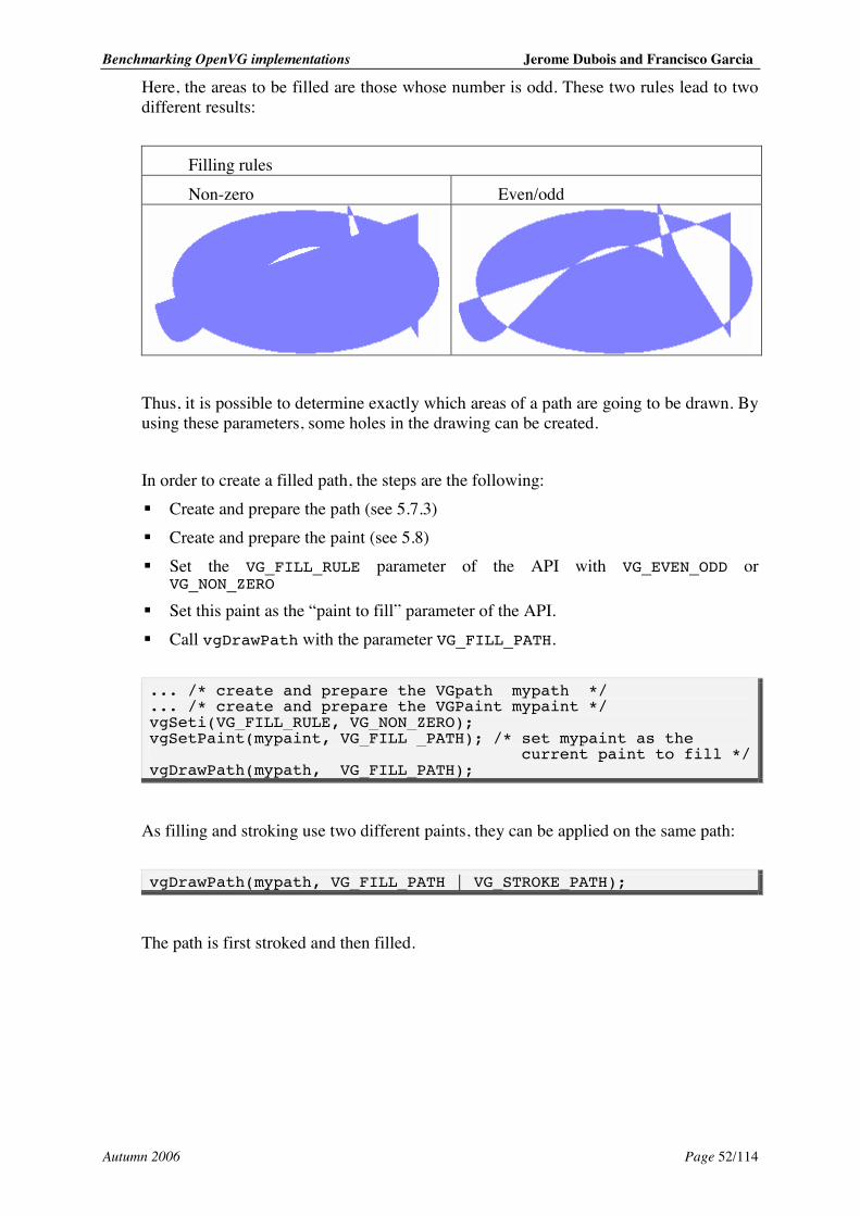
Benchmarking OpenVG implementations Jerome Dubois and Francisco Garcia
Autumn 2006 Page 52/114
Here, the areas to be filled are those whose number is odd. These two rules lead to two different results:
Filling rules
Non-zero Even/odd
Thus, it is possible to determine exactly which areas of a path are going to be drawn. By using these parameters, some holes in the drawing can be created. In order to create a filled path, the steps are the following: ! Create and prepare the path (see 5.7.3) ! Create and prepare the paint (see 5.8) ! Set the VG_FILL_RULE parameter of the API with VG_EVEN_ODD or
VG_NON_ZERO ! Set this paint as the “paint to fill” parameter of the API. ! Call vgDrawPath with the parameter VG_FILL_PATH. ... /* create and prepare the VGpath mypath */ ... /* create and prepare the VGPaint mypaint */ vgSeti(VG_FILL_RULE, VG_NON_ZERO); vgSetPaint(mypaint, VG_FILL _PATH); /* set mypaint as the current paint to fill */ vgDrawPath(mypath, VG_FILL_PATH);
As filling and stroking use two different paints, they can be applied on the same path: vgDrawPath(mypath, VG_FILL_PATH | VG_STROKE_PATH);
The path is first stroked and then filled.
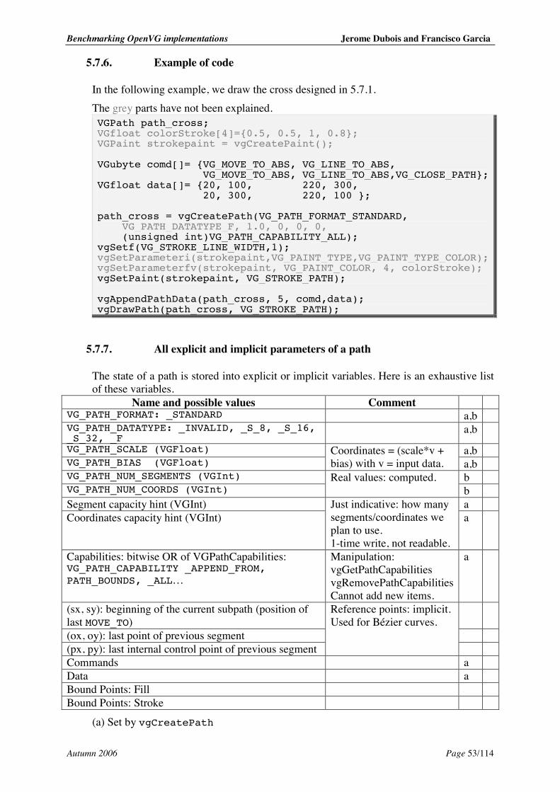
Benchmarking OpenVG implementations Jerome Dubois and Francisco Garcia
Autumn 2006 Page 53/114
5.7.6. Example of code
In the following example, we draw the cross designed in 5.7.1. The grey parts have not been explained. VGPath path_cross; VGfloat colorStroke[4]={0.5, 0.5, 1, 0.8}; VGPaint strokepaint = vgCreatePaint(); VGubyte comd[]= {VG_MOVE_TO_ABS, VG_LINE_TO_ABS, VG_MOVE_TO_ABS, VG_LINE_TO_ABS,VG_CLOSE_PATH}; VGfloat data[]= {20, 100, 220, 300, 20, 300, 220, 100 }; path_cross = vgCreatePath(VG_PATH_FORMAT_STANDARD, VG_PATH_DATATYPE_F, 1.0, 0, 0, 0, (unsigned int)VG_PATH_CAPABILITY_ALL); vgSetf(VG_STROKE_LINE_WIDTH,1); vgSetParameteri(strokepaint,VG_PAINT_TYPE,VG_PAINT_TYPE_COLOR); vgSetParameterfv(strokepaint, VG_PAINT_COLOR, 4, colorStroke); vgSetPaint(strokepaint, VG_STROKE_PATH); vgAppendPathData(path_cross, 5, comd,data); vgDrawPath(path_cross, VG_STROKE_PATH);
5.7.7. All explicit and implicit parameters of a path
The state of a path is stored into explicit or implicit variables. Here is an exhaustive list of these variables.
Name and possible values Comment VG_PATH_FORMAT: _STANDARD a,b VG_PATH_DATATYPE: _INVALID, _S_8, _S_16, _S_32, _F
a,b
VG_PATH_SCALE (VGFloat) a,b VG_PATH_BIAS (VGFloat)
Coordinates = (scale*v + bias) with v = input data. a,b
VG_PATH_NUM_SEGMENTS (VGInt) b VG_PATH_NUM_COORDS (VGInt)
Real values: computed. b
Segment capacity hint (VGInt) a Coordinates capacity hint (VGInt)
Just indicative: how many segments/coordinates we plan to use. 1-time write, not readable.
a
Capabilities: bitwise OR of VGPathCapabilities: VG_PATH_CAPABILITY _APPEND_FROM, PATH_BOUNDS, _ALL…
Manipulation: vgGetPathCapabilities vgRemovePathCapabilities Cannot add new items.
a
(sx, sy): beginning of the current subpath (position of last MOVE_TO)
(ox, oy): last point of previous segment (px, py): last internal control point of previous segment
Reference points: implicit. Used for Bézier curves.
Commands a Data a Bound Points: Fill Bound Points: Stroke
(a) Set by vgCreatePath
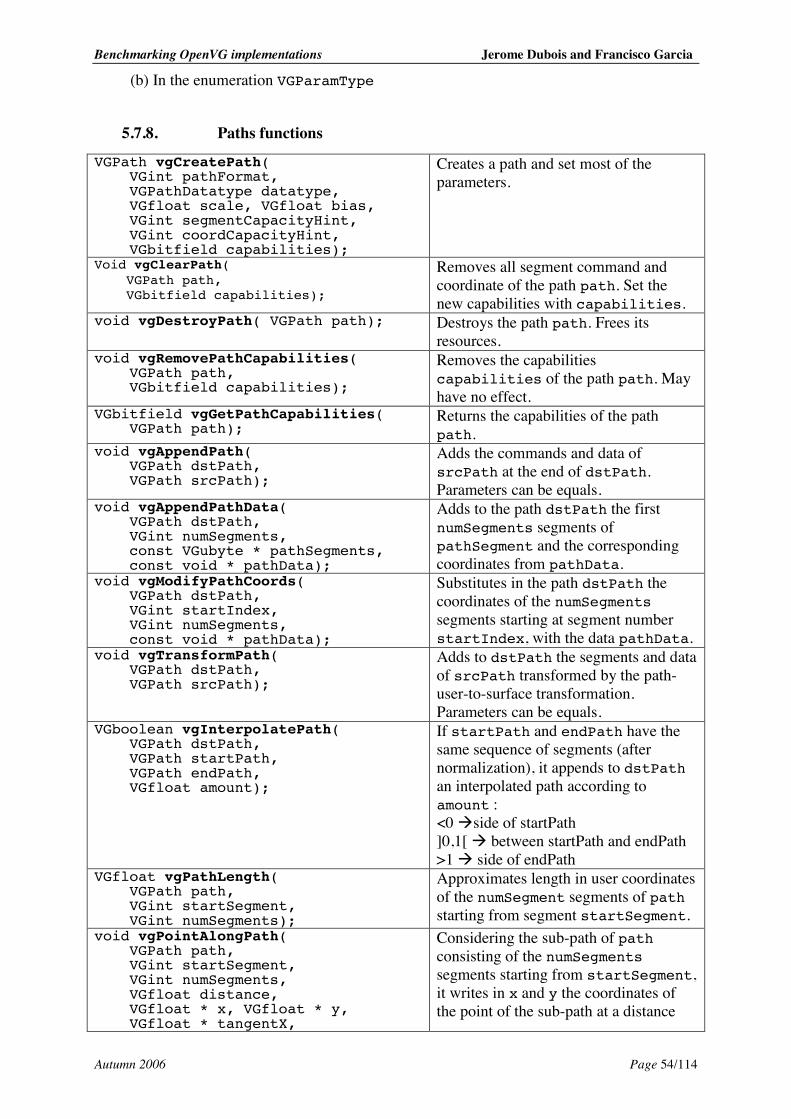
Benchmarking OpenVG implementations Jerome Dubois and Francisco Garcia
Autumn 2006 Page 54/114
(b) In the enumeration VGParamType
5.7.8. Paths functions
VGPath vgCreatePath( VGint pathFormat, VGPathDatatype datatype, VGfloat scale, VGfloat bias, VGint segmentCapacityHint, VGint coordCapacityHint, VGbitfield capabilities);
Creates a path and set most of the parameters.
Void vgClearPath( VGPath path, VGbitfield capabilities);
Removes all segment command and coordinate of the path path. Set the new capabilities with capabilities.
void vgDestroyPath( VGPath path); Destroys the path path. Frees its resources.
void vgRemovePathCapabilities( VGPath path, VGbitfield capabilities);
Removes the capabilities capabilities of the path path. May have no effect.
VGbitfield vgGetPathCapabilities( VGPath path);
Returns the capabilities of the path path.
void vgAppendPath( VGPath dstPath, VGPath srcPath);
Adds the commands and data of srcPath at the end of dstPath. Parameters can be equals.
void vgAppendPathData( VGPath dstPath, VGint numSegments, const VGubyte * pathSegments, const void * pathData);
Adds to the path dstPath the first numSegments segments of pathSegment and the corresponding coordinates from pathData.
void vgModifyPathCoords( VGPath dstPath, VGint startIndex, VGint numSegments, const void * pathData);
Substitutes in the path dstPath the coordinates of the numSegments segments starting at segment number startIndex, with the data pathData.
void vgTransformPath( VGPath dstPath, VGPath srcPath);
Adds to dstPath the segments and data of srcPath transformed by the path-user-to-surface transformation. Parameters can be equals.
VGboolean vgInterpolatePath( VGPath dstPath, VGPath startPath, VGPath endPath, VGfloat amount);
If startPath and endPath have the same sequence of segments (after normalization), it appends to dstPath an interpolated path according to amount : <0 "side of startPath ]0,1[ " between startPath and endPath >1 " side of endPath
VGfloat vgPathLength( VGPath path, VGint startSegment, VGint numSegments);
Approximates length in user coordinates of the numSegment segments of path starting from segment startSegment.
void vgPointAlongPath( VGPath path, VGint startSegment, VGint numSegments, VGfloat distance, VGfloat * x, VGfloat * y, VGfloat * tangentX,
Considering the sub-path of path consisting of the numSegments segments starting from startSegment, it writes in x and y the coordinates of the point of the sub-path at a distance
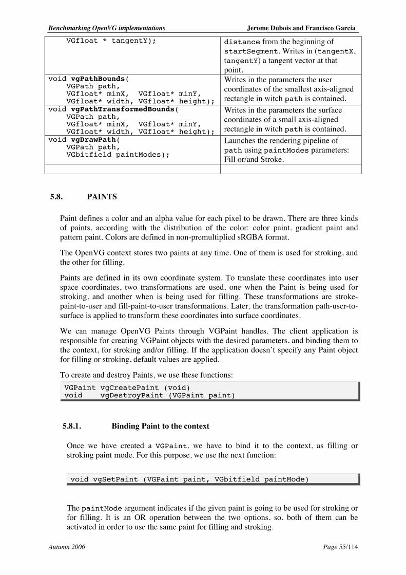
Benchmarking OpenVG implementations Jerome Dubois and Francisco Garcia
Autumn 2006 Page 55/114
VGfloat * tangentY); distance from the beginning of startSegment. Writes in (tangentX, tangentY) a tangent vector at that point.
void vgPathBounds( VGPath path, VGfloat* minX, VGfloat* minY, VGfloat* width, VGfloat* height);
Writes in the parameters the user coordinates of the smallest axis-aligned rectangle in witch path is contained.
void vgPathTransformedBounds( VGPath path, VGfloat* minX, VGfloat* minY, VGfloat* width, VGfloat* height);
Writes in the parameters the surface coordinates of a small axis-aligned rectangle in witch path is contained.
void vgDrawPath( VGPath path, VGbitfield paintModes);
Launches the rendering pipeline of path using paintModes parameters: Fill or/and Stroke.
5.8. PAINTS
Paint defines a color and an alpha value for each pixel to be drawn. There are three kinds of paints, according with the distribution of the color: color paint, gradient paint and pattern paint. Colors are defined in non-premultiplied sRGBA format.
The OpenVG context stores two paints at any time. One of them is used for stroking, and the other for filling.
Paints are defined in its own coordinate system. To translate these coordinates into user space coordinates, two transformations are used, one when the Paint is being used for stroking, and another when is being used for filling. These transformations are stroke-paint-to-user and fill-paint-to-user transformations. Later, the transformation path-user-to-surface is applied to transform these coordinates into surface coordinates.
We can manage OpenVG Paints through VGPaint handles. The client application is responsible for creating VGPaint objects with the desired parameters, and binding them to the context, for stroking and/or filling. If the application doesn’t specify any Paint object for filling or stroking, default values are applied.
To create and destroy Paints, we use these functions: VGPaint vgCreatePaint (void) void vgDestroyPaint (VGPaint paint)
5.8.1. Binding Paint to the context
Once we have created a VGPaint, we have to bind it to the context, as filling or stroking paint mode. For this purpose, we use the next function: void vgSetPaint (VGPaint paint, VGbitfield paintMode)
The paintMode argument indicates if the given paint is going to be used for stroking or for filling. It is an OR operation between the two options, so, both of them can be activated in order to use the same paint for filling and stroking.
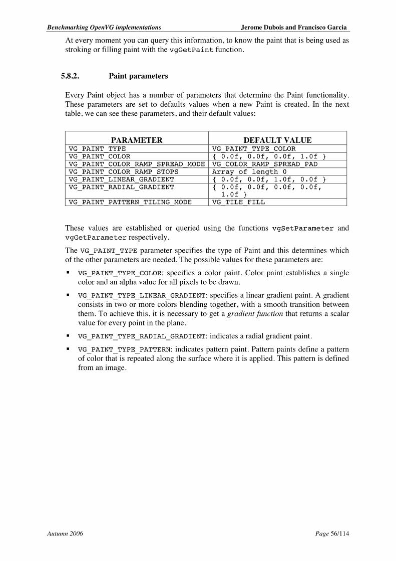
Benchmarking OpenVG implementations Jerome Dubois and Francisco Garcia
Autumn 2006 Page 56/114
At every moment you can query this information, to know the paint that is being used as stroking or filling paint with the vgGetPaint function.
5.8.2. Paint parameters
Every Paint object has a number of parameters that determine the Paint functionality. These parameters are set to defaults values when a new Paint is created. In the next table, we can see these parameters, and their default values:
PARAMETER DEFAULT VALUE VG_PAINT_TYPE VG_PAINT_TYPE_COLOR VG_PAINT_COLOR { 0.0f, 0.0f, 0.0f, 1.0f } VG_PAINT_COLOR_RAMP_SPREAD_MODE VG_COLOR_RAMP_SPREAD_PAD VG_PAINT_COLOR_RAMP_STOPS Array of length 0 VG_PAINT_LINEAR_GRADIENT { 0.0f, 0.0f, 1.0f, 0.0f } VG_PAINT_RADIAL_GRADIENT { 0.0f, 0.0f, 0.0f, 0.0f,
1.0f } VG_PAINT_PATTERN_TILING_MODE VG_TILE_FILL
These values are established or queried using the functions vgSetParameter and vgGetParameter respectively. The VG_PAINT_TYPE parameter specifies the type of Paint and this determines which of the other parameters are needed. The possible values for these parameters are: ! VG_PAINT_TYPE_COLOR: specifies a color paint. Color paint establishes a single
color and an alpha value for all pixels to be drawn. ! VG_PAINT_TYPE_LINEAR_GRADIENT: specifies a linear gradient paint. A gradient
consists in two or more colors blending together, with a smooth transition between them. To achieve this, it is necessary to get a gradient function that returns a scalar value for every point in the plane.
! VG_PAINT_TYPE_RADIAL_GRADIENT: indicates a radial gradient paint. ! VG_PAINT_TYPE_PATTERN: indicates pattern paint. Pattern paints define a pattern
of color that is repeated along the surface where it is applied. This pattern is defined from an image.
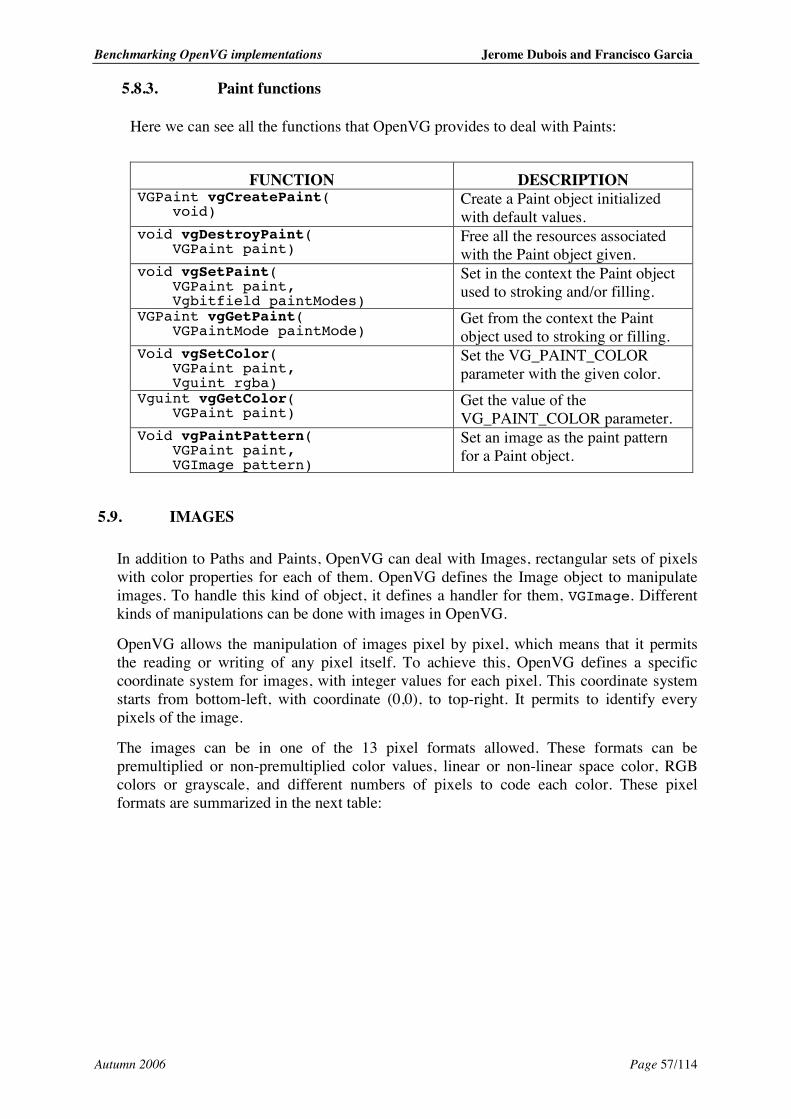
Benchmarking OpenVG implementations Jerome Dubois and Francisco Garcia
Autumn 2006 Page 57/114
5.8.3. Paint functions
Here we can see all the functions that OpenVG provides to deal with Paints:
FUNCTION DESCRIPTION VGPaint vgCreatePaint( void)
Create a Paint object initialized with default values.
void vgDestroyPaint( VGPaint paint)
Free all the resources associated with the Paint object given.
void vgSetPaint( VGPaint paint, Vgbitfield paintModes)
Set in the context the Paint object used to stroking and/or filling.
VGPaint vgGetPaint( VGPaintMode paintMode)
Get from the context the Paint object used to stroking or filling.
Void vgSetColor( VGPaint paint, Vguint rgba)
Set the VG_PAINT_COLOR parameter with the given color.
Vguint vgGetColor( VGPaint paint)
Get the value of the VG_PAINT_COLOR parameter.
Void vgPaintPattern( VGPaint paint, VGImage pattern)
Set an image as the paint pattern for a Paint object.
5.9. IMAGES
In addition to Paths and Paints, OpenVG can deal with Images, rectangular sets of pixels with color properties for each of them. OpenVG defines the Image object to manipulate images. To handle this kind of object, it defines a handler for them, VGImage. Different kinds of manipulations can be done with images in OpenVG.
OpenVG allows the manipulation of images pixel by pixel, which means that it permits the reading or writing of any pixel itself. To achieve this, OpenVG defines a specific coordinate system for images, with integer values for each pixel. This coordinate system starts from bottom-left, with coordinate (0,0), to top-right. It permits to identify every pixels of the image.
The images can be in one of the 13 pixel formats allowed. These formats can be premultiplied or non-premultiplied color values, linear or non-linear space color, RGB colors or grayscale, and different numbers of pixels to code each color. These pixel formats are summarized in the next table:
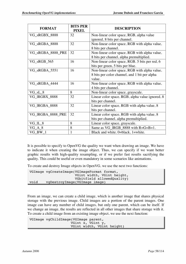
Benchmarking OpenVG implementations Jerome Dubois and Francisco Garcia
Autumn 2006 Page 58/114
FORMAT BITS PER PIXEL DESCRIPTION
VG_sRGBX_8888 32 Non-linear color space, RGB, alpha value ignored, 8 bits per channel.
VG_sRGBA_8888 32 Non-linear color space, RGB with alpha value, 8 bits per channel.
VG_sRGBA_8888_PRE 32 Non-linear color space, RGB with alpha value, 8 bits per channel, alpha premultiplied.
VG_sRGB_565 16 Non-linear color space, RGB. 5 bits per red, 6 bits per green, 5 bits per blue.
VG_sRGBA_5551 16 Non-linear color space, RGB with alpha value, 8 bits per color channel, and 1 bit per alpha value.
VG_sRGBA_4444 16 Non-linear color space, RGB with alpha value, 4 bits per channel.
VG_sL_8 8 Non-linear color space, grayscale. VG_lRGBX_8888 32 Linear color space, RGB, alpha value ignored, 8
bits per channel. VG_lRGBA_8888 32 Linear color space, RGB with alpha value, 8
bits per channel. VG_lRGBA_8888_PRE 32 Linear color space, RGB with alpha value, 8
bits per channel, alpha premultiplied. VG_lL_8 8 Linear color space, grayscale. VG_A_8 8 Same as VG_lRGB_8888 with R=G=B=1. VG_BW_1 1 Black and white. 0=black, 1=white.
It is possible to specify to OpenVG the quality we want when drawing an image. We have to indicate it when creating the image object. Thus, we can specify if we want better graphic results with high-quality resampling, or if we prefer fast results sacrifying the quality. This could be useful or even mandatory in some scenarios like animations.
To create and destroy Image objects in OpenVG, we use the next two functions: VGImage vgCreateImage(VGImageFormat format, VGint width, VGint height, VGbitfield allowedQuality) void vgDestroyImage(VGImage image)
From an image, we can create a child image, which is another image that shares physical storage with the previous image. Child images are a portion of the parent images. One image can have any number of child images, but only one parent, which can be itself. If we change an image, the results are reflected in all other images that share storage with it. To create a child image from an existing image object, we use the next function: VGImage vgChildImage(VGImage parent, VGint x, VGint y, VGint width, VGint height)
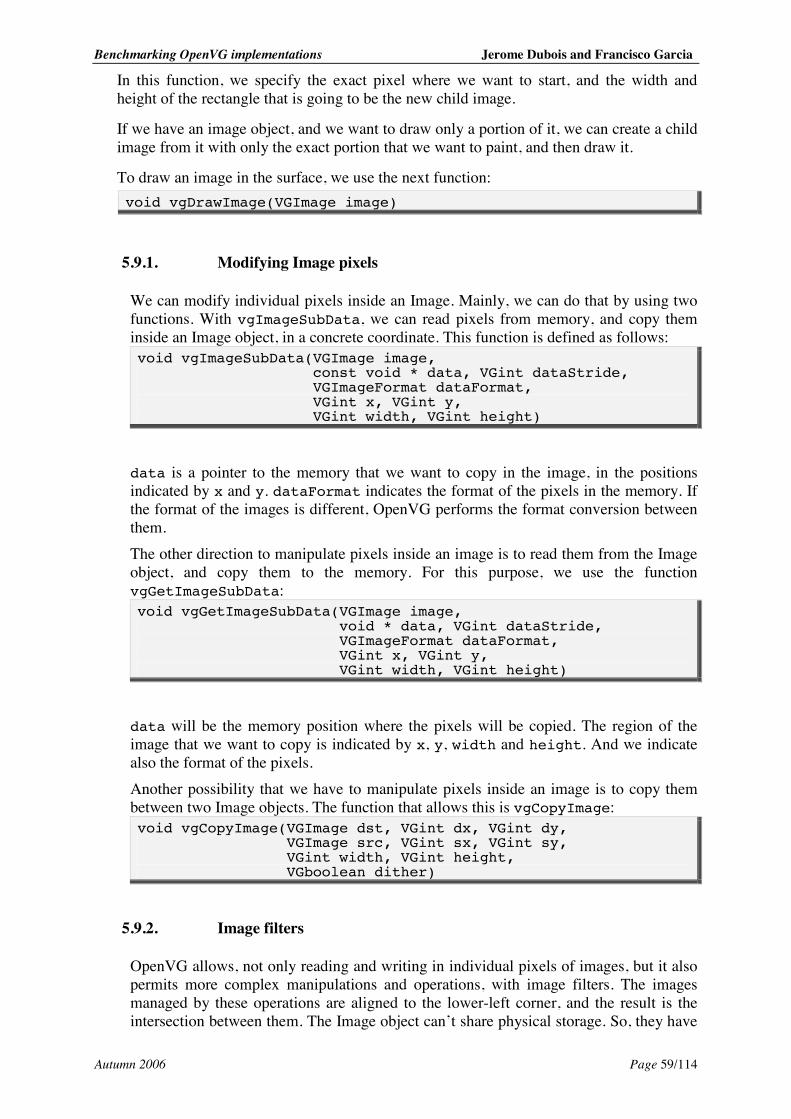
Benchmarking OpenVG implementations Jerome Dubois and Francisco Garcia
Autumn 2006 Page 59/114
In this function, we specify the exact pixel where we want to start, and the width and height of the rectangle that is going to be the new child image.
If we have an image object, and we want to draw only a portion of it, we can create a child image from it with only the exact portion that we want to paint, and then draw it.
To draw an image in the surface, we use the next function: void vgDrawImage(VGImage image)
5.9.1. Modifying Image pixels
We can modify individual pixels inside an Image. Mainly, we can do that by using two functions. With vgImageSubData, we can read pixels from memory, and copy them inside an Image object, in a concrete coordinate. This function is defined as follows: void vgImageSubData(VGImage image, const void * data, VGint dataStride, VGImageFormat dataFormat, VGint x, VGint y, VGint width, VGint height)
data is a pointer to the memory that we want to copy in the image, in the positions indicated by x and y. dataFormat indicates the format of the pixels in the memory. If the format of the images is different, OpenVG performs the format conversion between them. The other direction to manipulate pixels inside an image is to read them from the Image object, and copy them to the memory. For this purpose, we use the function vgGetImageSubData: void vgGetImageSubData(VGImage image, void * data, VGint dataStride, VGImageFormat dataFormat, VGint x, VGint y, VGint width, VGint height)
data will be the memory position where the pixels will be copied. The region of the image that we want to copy is indicated by x, y, width and height. And we indicate also the format of the pixels. Another possibility that we have to manipulate pixels inside an image is to copy them between two Image objects. The function that allows this is vgCopyImage: void vgCopyImage(VGImage dst, VGint dx, VGint dy, VGImage src, VGint sx, VGint sy, VGint width, VGint height, VGboolean dither)
5.9.2. Image filters
OpenVG allows, not only reading and writing in individual pixels of images, but it also permits more complex manipulations and operations, with image filters. The images managed by these operations are aligned to the lower-left corner, and the result is the intersection between them. The Image object can’t share physical storage. So, they have
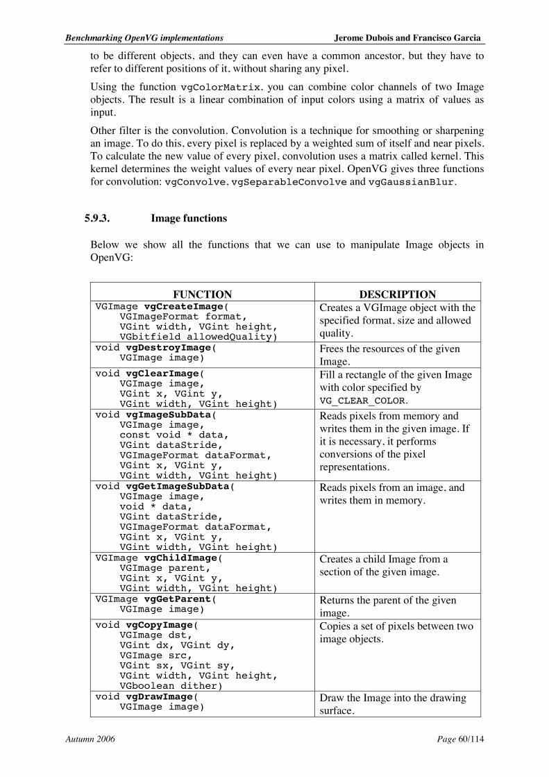
Benchmarking OpenVG implementations Jerome Dubois and Francisco Garcia
Autumn 2006 Page 60/114
to be different objects, and they can even have a common ancestor, but they have to refer to different positions of it, without sharing any pixel. Using the function vgColorMatrix, you can combine color channels of two Image objects. The result is a linear combination of input colors using a matrix of values as input. Other filter is the convolution. Convolution is a technique for smoothing or sharpening an image. To do this, every pixel is replaced by a weighted sum of itself and near pixels. To calculate the new value of every pixel, convolution uses a matrix called kernel. This kernel determines the weight values of every near pixel. OpenVG gives three functions for convolution: vgConvolve, vgSeparableConvolve and vgGaussianBlur.
5.9.3. Image functions
Below we show all the functions that we can use to manipulate Image objects in OpenVG:
FUNCTION DESCRIPTION VGImage vgCreateImage( VGImageFormat format, VGint width, VGint height, VGbitfield allowedQuality)
Creates a VGImage object with the specified format, size and allowed quality.
void vgDestroyImage( VGImage image)
Frees the resources of the given Image.
void vgClearImage( VGImage image, VGint x, VGint y, VGint width, VGint height)
Fill a rectangle of the given Image with color specified by VG_CLEAR_COLOR.
void vgImageSubData( VGImage image, const void * data, VGint dataStride, VGImageFormat dataFormat, VGint x, VGint y, VGint width, VGint height)
Reads pixels from memory and writes them in the given image. If it is necessary, it performs conversions of the pixel representations.
void vgGetImageSubData( VGImage image, void * data, VGint dataStride, VGImageFormat dataFormat, VGint x, VGint y, VGint width, VGint height)
Reads pixels from an image, and writes them in memory.
VGImage vgChildImage( VGImage parent, VGint x, VGint y, VGint width, VGint height)
Creates a child Image from a section of the given image.
VGImage vgGetParent( VGImage image)
Returns the parent of the given image.
void vgCopyImage( VGImage dst, VGint dx, VGint dy, VGImage src, VGint sx, VGint sy, VGint width, VGint height, VGboolean dither)
Copies a set of pixels between two image objects.
void vgDrawImage( VGImage image)
Draw the Image into the drawing surface.
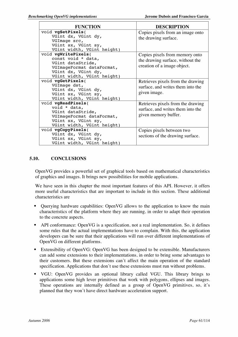
Benchmarking OpenVG implementations Jerome Dubois and Francisco Garcia
Autumn 2006 Page 61/114
FUNCTION DESCRIPTION void vgSetPixels( VGint dx, VGint dy, VGImage src, VGint sx, VGint sy, VGint width, VGint height)
Copies pixels from an image onto the drawing surface.
void vgWritePixels( const void * data, VGint dataStride, VGImageFormat dataFormat, VGint dx, VGint dy, VGint width, VGint height)
Copies pixels from memory onto the drawing surface, without the creation of a image object.
void vgGetPixels( VGImage dst, VGint dx, VGint dy, VGint sx, VGint sy, VGint width, VGint height)
Retrieves pixels from the drawing surface, and writes them into the given image.
void vgReadPixels( void * data, VGint dataStride, VGImageFormat dataFormat, VGint sx, VGint sy, VGint width, VGint height)
Retrieves pixels from the drawing surface, and writes them into the given memory buffer.
void vgCopyPixels( VGint dx, VGint dy, VGint sx, VGint sy, VGint width, VGint height)
Copies pixels between two sections of the drawing surface.
5.10. CONCLUSIONS
OpenVG provides a powerful set of graphical tools based on mathematical characteristics of graphics and images. It brings new possibilities for mobile applications.
We have seen in this chapter the most important features of this API. However, it offers more useful characteristics that are important to include in this section. These additional characteristics are
! Querying hardware capabilities: OpenVG allows to the application to know the main characteristics of the platform where they are running, in order to adapt their operation to the concrete aspects.
! API conformance: OpenVG is a specification, not a real implementation. So, it defines some rules that the actual implementations have to complain. With this, the application developers can be sure that their applications will run over different implementations of OpenVG on different platforms.
! Extensibility of OpenVG: OpenVG has been designed to be extensible. Manufacturers can add some extensions to their implementations, in order to bring some advantages to their customers. But these extensions can’t affect the main operation of the standard specification. Applications that don’t use these extensions must run without problems.
! VGU: OpenVG provides an optional library called VGU. This library brings to applications some high lever primitives that work with polygons, ellipses and images. These operations are internally defined as a group of OpenVG primitives, so, it’s planned that they won’t have direct hardware acceleration support.
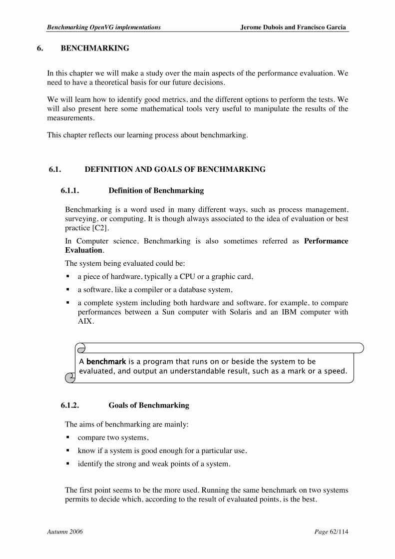
Benchmarking OpenVG implementations Jerome Dubois and Francisco Garcia
Autumn 2006 Page 62/114
6. BENCHMARKING
In this chapter we will make a study over the main aspects of the performance evaluation. We need to have a theoretical basis for our future decisions.
We will learn how to identify good metrics, and the different options to perform the tests. We will also present here some mathematical tools very useful to manipulate the results of the measurements.
This chapter reflects our learning process about benchmarking.
6.1. DEFINITION AND GOALS OF BENCHMARKING
6.1.1. Definition of Benchmarking
Benchmarking is a word used in many different ways, such as process management, surveying, or computing. It is though always associated to the idea of evaluation or best practice [C2]. In Computer science, Benchmarking is also sometimes referred as Performance Evaluation. The system being evaluated could be: ! a piece of hardware, typically a CPU or a graphic card, ! a software, like a compiler or a database system, ! a complete system including both hardware and software, for example, to compare
performances between a Sun computer with Solaris and an IBM computer with AIX.
6.1.2. Goals of Benchmarking
The aims of benchmarking are mainly: ! compare two systems, ! know if a system is good enough for a particular use, ! identify the strong and weak points of a system. The first point seems to be the more used. Running the same benchmark on two systems permits to decide which, according to the result of evaluated points, is the best.
Benchmarking OpenVG implementations Jerome Dubois and Francisco Garcia
Autumn 2006 Page 63/114
The second aim doesn’t care about best performances, but only tries to find out if a particular system will fit the needs. The last point is used when the developers of a system want to know which part of the system they should try to improve. The two first goals are for the client side, and the third is for the developer side.
6.1.3. Need for a reference
In all cases, we need a reference. The outputs of a benchmark mean nothing, if they cannot be compared with those from another system or with an average result. If we measure 200 Kg of snow on a tree, we cannot say if it’s much or few if we have no clue about other trees. Back in computer field, let us have another example: a graphical API. If we say “this system can draw 300 triangles per second”, it’s hard to say if it’s a revolutionary or a very poor system if we don’t know average performances of such systems. This need for a reference is even truer if the output does not correspond to an easy understandable unity. For example, if the benchmark measures hundred or thousand of different aspects of a system (time to draw 200 lines, time to draw 100 circles, power consumption, and clock frequency) and outputs as unique result a general mark computed from these measurements, we need a reference to compare. A mark of 645 is nice if another system has 612, but very poor if the average mark is 4200.
6.1.4. Performance evaluation and Benchmarking
Performance analysis and benchmarking are very close. David J.Lilja defines performance analysis as “a combination of measurement, interpretation, and communication of a computer system’s ‘speed’ or ‘size’ (sometimes referred to as its ‘capacity’)”[C1]. He presents three techniques for performance analysis: ! Measurement ! Simulation ! Analytical modeling Although simulation and analytical modeling can be invaluable tools, benchmarking includes only measurements. Thus, we can say that Benchmarking is a sub-part of performance evaluation. It is the one to be used when the system is available.
6.2. NEUTRAL POINT OF VIEW AND BENCHMARK BUSINESS
Imagine a benchmark which measures two things:
! A: time to draw 200 lines ! B: number of circles drawn in 2 seconds
Benchmarking OpenVG implementations Jerome Dubois and Francisco Garcia
Autumn 2006 Page 64/114
The final output of this benchmark can be a mark M compute as BAM .. βα +=
Imagine now two competitor system providers working together on this benchmark. The system from the first is quite good at drawing lines, and the second at drawing circles. Sure, the first provider will want a high value of , and a low value of , which the other system provider will object to.
This example shows that people should investigate about benchmark before trusting them. In particular, a benchmark provided by the same company than the product is most of the time not neutral.
Comparing system performances is so important that there is a need for well known benchmarks. These are produced either by an independent company, or by a consortium of competitors. Lobbying exists in both cases. Benchmark lobbying and other practices to show products under a good light is called bench-marketing.
Thus, a good benchmark is system neutral, and people should not trust a benchmark without investigating about it before. Of course, being open-source is a quality for a benchmark, since it allows everybody to check how the benchmark works.
6.3. METRICS
When we talk about performance evaluation and benchmarking, we are talking about comparing different systems to know which one has the better performances. In order to do this, we need to know what things are interesting to measure. The results of these measurements will be used to know which system is better. These values, results of the measurements, are the performance metrics.
In order to make a good evaluation, we need to identify the correct metrics to use in the comparison. A bad metric can not only make difficult the decision process, but could give wrong results and can even make the worst system seeming to be the best. So, in the process of performance evaluation, the identification of the metrics to be used is extremely important to reach good results.
To obtain the metrics, there are different strategies:
! Fixed load of work, and measurement of the execution time. ! Fixed execution time, and measurement of the work done. ! Variable load of work and variable execution time, and measurement of the size of
some different parameters. Sometimes, we can be interested in these values directly. In this case, we can use the results of the measurements directly, without making any transformation. But in other cases, we need to normalize these values to a common time basis, in order to obtain better values to make comparisons. This type of metrics is called rate metric or throughput.
6.3.1. Characteristics of a good performance metric
When we are going to compare different systems, we can use a big set of different metrics to do it. But it is clear that not all of them are good for our purpose. A bad selection of the metrics to use can lead us to erroneous conclusions. Thus, we need a
Benchmarking OpenVG implementations Jerome Dubois and Francisco Garcia
Autumn 2006 Page 65/114
way to identify a good metric for every case, that can help us to make a good comparison, and that we can interpret correctly. It is possible to enumerate the desired characteristics that can tell us if a metric is a good metric or not. Although these characteristics are desirable, a metric could be a good metric without fulfilling all of them. However, using a metric that doesn’t fulfill any characteristic, could lead to erroneous conclusions. These characteristics are: ! Linearity: If, when the value of the metric changes by a certain ratio, the real
performance of the system changes with the same ratio, then the metric is linear. This characteristic is desirable because it helps the human mind to understand better the meaning of the metric, and how to use it.
! Reliability: A performance metric is reliable if the fact that we always obtain a better result of this metric in one system, comparing with others, means that this system really outperforms the others. This characteristic is really important to obtain useful metrics that can be used to compare different systems.
! Repeatability: If every time that the test is executed, we obtain the same result for the metric, then that performance metric is repeatable.
! Easiness of measurement: If a metric is difficult to measure, then it is not a good metric to evaluate systems, since it is not easy for the analysts to use it, and the probability to make a mistake can be very high. A metric measured incorrectly could be very prejudicial, since it gives wrong conclusions that can be hard to detect.
! Consistency: A performance metric is consistent if it uses the same unit and precision in every system and every configuration. If a performance metric uses different units for two systems, we could not compare them because they are not the same thing.
! Independence: Many people use the results of performance metrics as a help in the decision for purchasing new computers. This prompts computers manufacturers to design their systems to obtain better results in some important metrics although this doesn’t imply that the system is really better. Also, the manufacturers can influent the composition of the metrics to achieve better results with it. So, it is very important that a good performance metric could be apart of these type of manipulations, and may be independent of manufacturers.
6.3.2. Example of metrics
Until now, different metrics have been used to make performance evaluation. Some of them have proved from experience being good metrics. Now we give examples of the main metrics used in actual practice to measure processor performances, and we can focus on the fulfillment of the desirable characteristics for a good metric. ! Clock rate: The processor clock rate is probably the most used metric to compare
systems for common people buying a new computer. But this is not a good metric. It ignores the memory architecture, or the I/O system, for example, and it’s impossible to give an accurate value of the performance of a system using only the frequency of the main clock. It is a metric repeatable, easy to measure, consistent, and is independent of the computer manufacturers. However, it doesn’t follow linearity
Benchmarking OpenVG implementations Jerome Dubois and Francisco Garcia
Autumn 2006 Page 66/114
and reliability. A system with a lower clock rate can achieve better results executing applications than another one with a higher value (e.g. AMD vs. Intel).
! MIPS: It is an acronym for millions of instructions per second. It is very easy to calculate this value. It responds to the next formula:
610×=
tnMIPS
where n is the number of instructions executed, and t is the time in seconds used to execute them. This metric is easy to measure, repeatable and independent. But it doesn’t carry out with the characteristics of linearity, reliability and consistency. The problem with this metric is that it uses the number of instructions as main value for the counter, and different processors can perform a different amount of work with one single instruction. Then, it has no sense to compare directly the number of instructions, like the clock rate as we saw previously. Thus, this is not a good metric to compare the performance.
! MFLOPS: It is an acronym for millions of floating-point operations per second. It uses the operations in floating point as basic unit to count. The formula is as follows:
610×=
tfMFLOPS
where f is the number of floating-point instructions executed in t seconds. The result in floating-point operations is better than simple instructions, like MIPS, to compare different systems. This is because floating point are less heterogeneous than simple instructions, and consequently, two different systems perform a similar load of work with this kind of instructions. So, we can note that MFLOPS is a better metric than MIPS. But this metric is still not a good metric, because it doesn’t respect reliability, consistency and independence.
! QUIPS: Quality improvement per second. It measures the quality of the solution achieved, instead of the effort. Quality concept has to be mathematically define on every concrete case, so, it’s possible to demonstrate the quality achieved. This is the reason why this metric is not always easy to measure, since sometimes it’s difficult to define the concept of quality. This metric complains with the characteristics of independency, consistency, repeatability, linearity, but is not always reliable.
6.3.3. Speedup and relative change
Here we present two other metrics very useful to compare systems. They are normalized metrics, defined in terms of throughput or speed. These metrics are speedup and relative change. ! Speedup: if we have two different speed metrics Ra and Rb, from two different
systems A and B, the speedup is the value S that respect: RbSRa ×=
We can say that system A is S times faster than system B. A speed metric can be expressed as Ra = Da/Ta. The speedup of the system A compared with the system B could be expressed as:
Benchmarking OpenVG implementations Jerome Dubois and Francisco Garcia
Autumn 2006 Page 67/114
a
b
b
a
b
aba T
TTDTD
RR
S ===//
,
! Relative change: a good way to compare the performance of two systems is to express the performance of one system as a percentage of the other. We define the relative change of the system A with respect to the system B as:
b
baba R
RR −=Δ ,
We can multiply this value by 100 to obtain a percentage of the relative change.
6.4. MEASUREMENTS
Once we know the best characteristics of the metrics, their importance, and how to use them, we need a process to obtain these metrics values. This process is the measuring of the values in which we are interested.
When considering measuring some aspects of a system, appears the concept of event. An event is something that occurs in the system, that changes its current state, and that we can detect. This concept is going to be the basis for our measurements, so it’s not useful if we can’t detect their occurrences. An event could be an arithmetic operation, the execution of a function, an access to a database, etc. The measurements are going to be always related to concrete events, defined previously, and the metrics are the way of using the values of the measurements to express the results.
The metrics can be classified in types according to the type of events that they consider. This classification is as follows:
! Event-count metrics: The simplest type of metrics is the count of how many times appears the event that we are measuring. For example, we can be interested in how many times an application writes on the disk.
! Secondary-event metrics: This type of metrics, records the value of a secondary parameter every time a concrete event occurs. An example of this type could be to record the memory status every time a calculation finishes.
! Profiles: These are aggregate metrics used to measure the performance of the whole system. This is used to identify possible bottlenecks.
With these types of events, there are different strategies that can be used to obtain the values of the measurements. The strategies are the ways to use the available tools to measure the events on which we focus.
According to Paul J. Fortier and Howard E. Michel, “Time is the most fundamental of concepts needed for computer systems performance analysis” [C3]. It is important to consider the time overhead (additional time that should not be part of the time measured) that is introduced in each method, since we need resources of the system to materialize the strategy in a real measurement. The analyst chooses the strategy considering the time and the type of events to be measured, in order to obtain the most accurate results.
The different types of strategies are:
Benchmarking OpenVG implementations Jerome Dubois and Francisco Garcia
Autumn 2006 Page 68/114
! Event-driven: This strategy for measuring the interesting values consists in recording the occurrences of the events in which we are interested every time they occur. We can have a counter for each of them. The analyst has to create the appropriate way of recording these occurrences of the event, and this task is not always easy, since it is sometimes necessary to access to very low level functionality, for example, in the case of recording the cache misses. This kind of benchmarking programs can add great level of overhead to the processing, since the consumption of resources is proportional to the number of times that the events occur. So, this strategy is recommended when the frequency of the events is not too high.
! Tracing: This strategy is very similar to event-driven strategy, but every time that an event occurs, we record sensible information related to the event. For example, when the event of cache miss occurs, we can record the data that we were requesting. This strategy consumes a higher quantity of resources, since it needs more storage space for recording the results, and more time to compute them.
! Sampling: This strategy uses an approach different than the event-driven strategies. With sampling strategy, we record valuable information useful for the measurement in fixed intervals of time, independent of the occurrences of the events. Of course, the analysts have to determine the correct frequency of sampling to obtain good results. With this approach, the overhead introduced for the measurement is independent of the number of occurrences of the events. It is only dependent of the duration of the test, and the frequency of the sampling. With sampling strategy we can obtain statistical information of the state of the system, since we can considerate that the events occurrences are asynchronous during the test.
! Indirect: It is sometimes not possible to measure the occurrences of an event. In this case, we can’t get the metric in which we are interested. The solution is to determine another metric that can be accessed and measured, and to derive the first one from this one. This is not always possible, and the analyst is the one in charge of finding a way to achieve it. We can say that this is a creative task that requires the experience and knowledge of the persons involved in the experiments.
With these strategies we can obtain different types of results, some of them more explicit than others. But, we have seen that the use of the instrumentation necessary to the measurement introduces an overhead and then, the results that we obtain are always different from the real results of the execution. If we need to record more information, we are probably going to use more system resources, and it then increases the overhead.
The most used tool for measuring is the interval timers. With this, we start a timer before the execution to be measured. Then, we do all the work, and finally, we stop the timer and obtain the total time used. Normally, when we start the timer, we really obtain a counter of the current ticks of a clock, and when we stop it, we obtain another counter. We only have to do a subtraction to obtain the real clock ticks used for the task, and multiply it for the duration of a tick. A part of this process is inside the recorded time. Therefore, the result is never the exact time used. In the next picture, we can see two intervals. The execution of the work to be measured is inside those intervals:
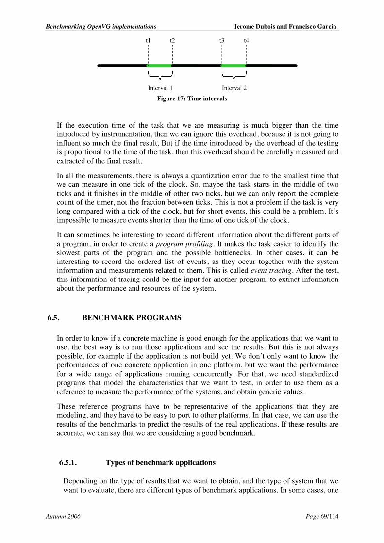
Benchmarking OpenVG implementations Jerome Dubois and Francisco Garcia
Autumn 2006 Page 69/114
Interval 1 terval
Interval 2
t1 t2 t3 t4
Figure 17: Time intervals
If the execution time of the task that we are measuring is much bigger than the time introduced by instrumentation, then we can ignore this overhead, because it is not going to influent so much the final result. But if the time introduced by the overhead of the testing is proportional to the time of the task, then this overhead should be carefully measured and extracted of the final result.
In all the measurements, there is always a quantization error due to the smallest time that we can measure in one tick of the clock. So, maybe the task starts in the middle of two ticks and it finishes in the middle of other two ticks, but we can only report the complete count of the timer, not the fraction between ticks. This is not a problem if the task is very long compared with a tick of the clock, but for short events, this could be a problem. It’s impossible to measure events shorter than the time of one tick of the clock.
It can sometimes be interesting to record different information about the different parts of a program, in order to create a program profiling. It makes the task easier to identify the slowest parts of the program and the possible bottlenecks. In other cases, it can be interesting to record the ordered list of events, as they occur together with the system information and measurements related to them. This is called event tracing. After the test, this information of tracing could be the input for another program, to extract information about the performance and resources of the system.
6.5. BENCHMARK PROGRAMS
In order to know if a concrete machine is good enough for the applications that we want to use, the best way is to run those applications and see the results. But this is not always possible, for example if the application is not build yet. We don’t only want to know the performances of one concrete application in one platform, but we want the performance for a wide range of applications running concurrently. For that, we need standardized programs that model the characteristics that we want to test, in order to use them as a reference to measure the performance of the systems, and obtain generic values.
These reference programs have to be representative of the applications that they are modeling, and they have to be easy to port to other platforms. In that case, we can use the results of the benchmarks to predict the results of the real applications. If these results are accurate, we can say that we are considering a good benchmark.
6.5.1. Types of benchmark applications
Depending on the type of results that we want to obtain, and the type of system that we want to evaluate, there are different types of benchmark applications. In some cases, one
Benchmarking OpenVG implementations Jerome Dubois and Francisco Garcia
Autumn 2006 Page 70/114
type could be more adequate than others to obtain the best results, since with each type we can run different kinds of experiments and we can focus on different aspects of the system to be measured. The principal types of benchmark programs are the following: ! Single instruction: This was the first way to compare computer’s performances, in
the beginning of the computation. Every instruction of the instruction set of one processor required the same execution time or cycles. The simplest test was to measure the time for one single instruction. The machine with the shorter execution time for one instruction was the fastest machine.
! Real programs: Some suits of benchmarks are constituted by a collection of real applications that have been considered as good programs to test different aspects of the performance of a system. These benchmarks can give very accurate information about the performance of the system. For example, real mathematical algorithms or algorithms for array ordering are typical types of applications used in common applications. With the time, an application can become useless to be used in a benchmark, because the problem it was dealing with has become instantaneous. There are two stages to develop benchmark suite using real programs:
! Selection of the applications that reveal to be useful for testing purposes. ! Values for the inputs: These inputs tend to be small set of data, in order to obtain
small execution times for the benchmark suite. This could lead to a negative impact in the accuracy of the benchmark.
! Synthetic benchmarks: This kind of benchmark applications tries to simulate the type and variety of instructions in real applications. They don’t do a real work, since they are built only for testing purposes, unlike applications in real programs. They try to use the same instruction set and same approaches, in order to obtain similar results of the execution. To build a synthetic benchmark, the analyst has to keep in mind the real applications that he wants to simulate and the system to be tested, in order to choose the correct instruction mixes.
! Program kernel benchmarks: These program benchmarks are used to test the main functionalities of an application. They are very small programs including the most important parts of real and bigger applications. These can be the most executed parts or the most time consuming. Due to the importance of this segment of code in the real application, measuring the performance of this portion can give a good approximation of the performance of the complete application. The problem with program kernel benchmarks arises from the same point than its strength: it focuses in a small part of the system, and ignores the rest. In a real system, it is very important when considering performance to know how the different parts of the system interact. Program kernel benchmarks have a limited application range nowadays.
! Micro benchmarks: This type of benchmark consists in very little and specific applications used to test the performance of different subsystems of a system. This type of benchmark is usually used to know the maximum performance that we can obtain from a concrete part of the system. This allows us to focus on the parts in which we are interested. For example, we can build tests to measure the processor performance, or the architecture memory performance.
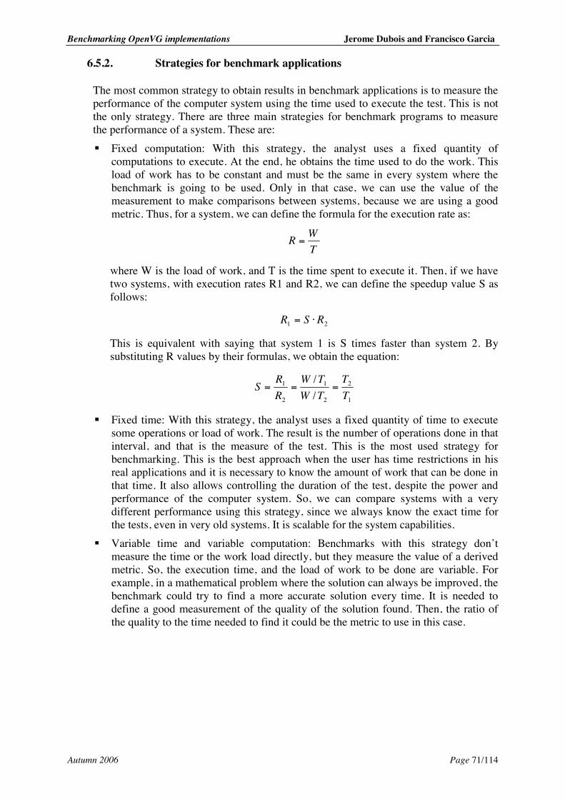
Benchmarking OpenVG implementations Jerome Dubois and Francisco Garcia
Autumn 2006 Page 71/114
6.5.2. Strategies for benchmark applications
The most common strategy to obtain results in benchmark applications is to measure the performance of the computer system using the time used to execute the test. This is not the only strategy. There are three main strategies for benchmark programs to measure the performance of a system. These are: ! Fixed computation: With this strategy, the analyst uses a fixed quantity of
computations to execute. At the end, he obtains the time used to do the work. This load of work has to be constant and must be the same in every system where the benchmark is going to be used. Only in that case, we can use the value of the measurement to make comparisons between systems, because we are using a good metric. Thus, for a system, we can define the formula for the execution rate as:
TWR =
where W is the load of work, and T is the time spent to execute it. Then, if we have two systems, with execution rates R1 and R2, we can define the speedup value S as follows:
21 RSR ⋅=
This is equivalent with saying that system 1 is S times faster than system 2. By substituting R values by their formulas, we obtain the equation:
1
2
2
1
2
1
//
TT
TWTW
RR
S ===
! Fixed time: With this strategy, the analyst uses a fixed quantity of time to execute some operations or load of work. The result is the number of operations done in that interval, and that is the measure of the test. This is the most used strategy for benchmarking. This is the best approach when the user has time restrictions in his real applications and it is necessary to know the amount of work that can be done in that time. It also allows controlling the duration of the test, despite the power and performance of the computer system. So, we can compare systems with a very different performance using this strategy, since we always know the exact time for the tests, even in very old systems. It is scalable for the system capabilities.
! Variable time and variable computation: Benchmarks with this strategy don’t measure the time or the work load directly, but they measure the value of a derived metric. So, the execution time, and the load of work to be done are variable. For example, in a mathematical problem where the solution can always be improved, the benchmark could try to find a more accurate solution every time. It is needed to define a good measurement of the quality of the solution found. Then, the ratio of the quality to the time needed to find it could be the metric to use in this case.
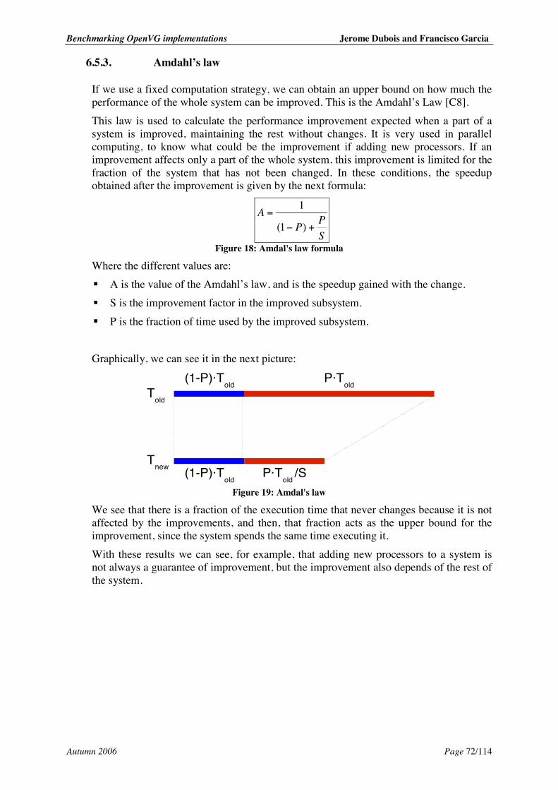
Benchmarking OpenVG implementations Jerome Dubois and Francisco Garcia
Autumn 2006 Page 72/114
6.5.3. Amdahl’s law
If we use a fixed computation strategy, we can obtain an upper bound on how much the performance of the whole system can be improved. This is the Amdahl’s Law [C8]. This law is used to calculate the performance improvement expected when a part of a system is improved, maintaining the rest without changes. It is very used in parallel computing, to know what could be the improvement if adding new processors. If an improvement affects only a part of the whole system, this improvement is limited for the fraction of the system that has not been changed. In these conditions, the speedup obtained after the improvement is given by the next formula:
SPP
A+−
=)1(
1
Figure 18: Amdal's law formula
Where the different values are: ! A is the value of the Amdahl’s law, and is the speedup gained with the change. ! S is the improvement factor in the improved subsystem. ! P is the fraction of time used by the improved subsystem. Graphically, we can see it in the next picture:
(1-P)·Told P·Told
Tnew
Told
(1-P)·Told P·Told /S Figure 19: Amdal's law
We see that there is a fraction of the execution time that never changes because it is not affected by the improvements, and then, that fraction acts as the upper bound for the improvement, since the system spends the same time executing it. With these results we can see, for example, that adding new processors to a system is not always a guarantee of improvement, but the improvement also depends of the rest of the system.
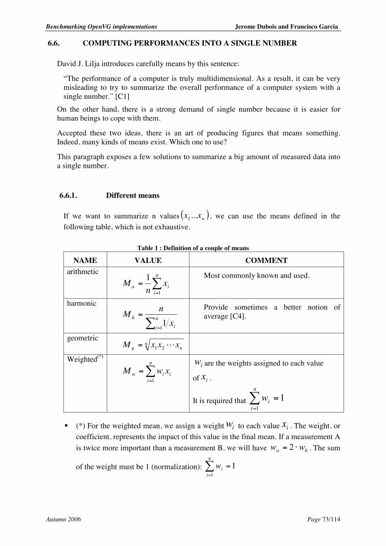
Benchmarking OpenVG implementations Jerome Dubois and Francisco Garcia
Autumn 2006 Page 73/114
6.6. COMPUTING PERFORMANCES INTO A SINGLE NUMBER
David J. Lilja introduces carefully means by this sentence:
“The performance of a computer is truly multidimensional. As a result, it can be very misleading to try to summarize the overall performance of a computer system with a single number.” [C1]
On the other hand, there is a strong demand of single number because it is easier for human beings to cope with them.
Accepted these two ideas, there is an art of producing figures that means something. Indeed, many kinds of means exist. Which one to use?
This paragraph exposes a few solutions to summarize a big amount of measured data into a single number.
6.6.1. Different means
If we want to summarize n values ( )nxx ...1 , we can use the means defined in the following table, which is not exhaustive.
Table 1 : Definition of a couple of means
NAME VALUE COMMENT arithmetic
=
=n
iia x
nM
1
1
Most commonly known and used.
harmonic
=
= n
i i
hx
nM11
Provide sometimes a better notion of average [C4].
geometric n
ng xxxM 21=
Weighted(*)
=
=n
iiiw xwM
1
iw are the weights assigned to each value
of ix .
It is required that 11
==
n
iiw
! (*) For the weighted mean, we assign a weight iw to each value ix . The weight, or coefficient, represents the impact of this value in the final mean. If a measurement A is twice more important than a measurement B, we will have ba ww ⋅= 2 . The sum
of the weight must be 1 (normalization): 11
==
n
iiw
Benchmarking OpenVG implementations Jerome Dubois and Francisco Garcia
Autumn 2006 Page 74/114
6.6.2. Choice of the method
The choice of the mean depends on the meaning of the values to be summarized. Moreover, as the mean is computed using values measured with a metric, it should respect the same characteristics.
If the metric of the ix is good, the mean will inherit the reliability, the repeatability, the easiness, and the consistency. Concerning the independence, this is subjective. It is true that the choice of the mean and of the coefficients, if they are used, is where companies can influence the result. The important characteristic to think about is the linearity.
If the considered metric is a time, the arithmetic mean is convenient, since aM is proportional to the total time, that is to say the performance. If we consider a rate, that is a number of events divided by a period of time, the harmonic mean can be used since it is proportional to the inverse of the sum of all times. The geographic mean can be used when the value range is wide, since it is less sensitive to extreme values than the arithmetic means. If this point is particularly important, the median can be used. The median is a number such as there is the same number of values bigger than smaller. If the number of values is odd, it is the average of the two middle values.
6.6.3. Think about
Reducing the quantity of information by combining many values into a single one requires carefulness. However, it helps comparison. Arithmetic and geographic means can be used for times, and harmonic mean should be used when considering rates. If we want to reduce values of different metrics and different meanings, the weighted mean can be used, though it introduces some subjectivity with the choice of the weight and compromises a perfect linearity. Finally, the most important to remember is that the final number should have the same characteristics than a good metric.
6.6.4. Statistical dispersion
In statistics, it is usual to use two indicators to represent a set of data: ! one for the localization – this indicator being typically a mean, and ! one for dispersion. The dispersion indicator gives an idea of how close to the mean the data are. If we consider the two sets of data (0, 100, 200) and (99, 100, 101), both have an arithmetic mean of 100. However, we see clearly that this value of 100 is not enough to represent the data. Indeed, the dispersion of the first set is much more important than the one of the second set.
Benchmarking OpenVG implementations Jerome Dubois and Francisco Garcia
Autumn 2006 Page 75/114
Many dispersion indicators exist[C6], but the most used are:
! the variance ( ) =−=
n
i i xxn
Var1
21, with ix the data and x the mean,
! the standard deviation Var=σ ,
! the coefficient of variation [C7]: MeanCV σ=
In the case of a benchmark, the data are the measurements, and the mean can be the final mark or an internal figure during the process of computing the final mark. The dispersion indicator gives a clue of the pertinence of the mean. If one of the data used for computing the mean is outstandingly high, the dispersion indicator will remind that in that case, the mean has a low pertinence. The user might want to run the benchmark again.
6.7. INTERPRETATION AND USE OF THE DATA MEASURED
Once the measurements have been done, it is not nice to provide the benchmark user with hundred pages of figures. It is a common thing to compute a reasonable amount of useful results. These results can be few figures representing marks, percentages, or other human understandable metric.
We can also think about other kinds of results, such as a single pass or fail mark, or a curve showing more in detail the response of the system while changing the stimuli. In car industry for example, car manufacturers feel obliged, and indeed are expected by clients, to provide a curve showing torque functions of engine speed.
People like when a benchmark provides a single figure, because it is easy to compare or to rank systems. However, one can want to have more detailed results, for example one per aspect of the system which has been measured. That is why it is a good idea that a benchmark can provide both, though most people are not interested by details.
Benchmarking OpenVG implementations Jerome Dubois and Francisco Garcia
Autumn 2006 Page 76/114
PART III.
BENCHMARK
DOCUMENTATION
In our work, we have made a separation between the benchmark framework and the tests.
! The task of the benchmark framework is to prepare and launch the tests, and then to print and compute the tests results to produce different levels and kinds of results.
! The task of the tests is to measure an aspect of the OpenVG implementation and return the result. There are about 3000 tests.
The next chapters describe our benchmark:
Chapter 7 Specifications What the benchmark should do? Why?
Chapter 8 Architecture How it works?
Chapter 9 Tests design What tests does the benchmark perform? How?
Chapter 10 Tests architecture How are the tests implemented?
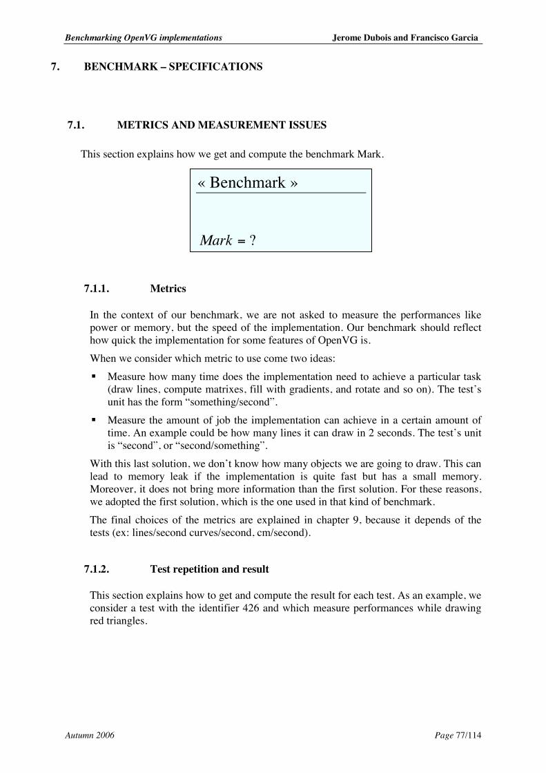
Benchmarking OpenVG implementations Jerome Dubois and Francisco Garcia
Autumn 2006 Page 77/114
7. BENCHMARK – SPECIFICATIONS
7.1. METRICS AND MEASUREMENT ISSUES
This section explains how we get and compute the benchmark Mark.
7.1.1. Metrics
In the context of our benchmark, we are not asked to measure the performances like power or memory, but the speed of the implementation. Our benchmark should reflect how quick the implementation for some features of OpenVG is. When we consider which metric to use come two ideas: ! Measure how many time does the implementation need to achieve a particular task
(draw lines, compute matrixes, fill with gradients, and rotate and so on). The test’s unit has the form “something/second”.
! Measure the amount of job the implementation can achieve in a certain amount of time. An example could be how many lines it can draw in 2 seconds. The test’s unit is “second”, or “second/something”.
With this last solution, we don’t know how many objects we are going to draw. This can lead to memory leak if the implementation is quite fast but has a small memory. Moreover, it does not bring more information than the first solution. For these reasons, we adopted the first solution, which is the one used in that kind of benchmark. The final choices of the metrics are explained in chapter 9, because it depends of the tests (ex: lines/second curves/second, cm/second).
7.1.2. Test repetition and result
This section explains how to get and compute the result for each test. As an example, we consider a test with the identifier 426 and which measure performances while drawing red triangles.
« Benchmark »
?=Mark
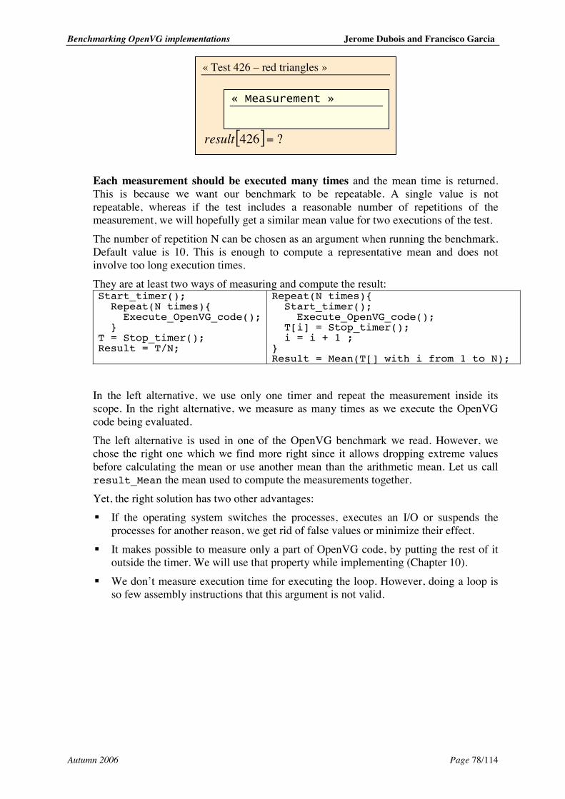
Benchmarking OpenVG implementations Jerome Dubois and Francisco Garcia
Autumn 2006 Page 78/114
Each measurement should be executed many times and the mean time is returned. This is because we want our benchmark to be repeatable. A single value is not repeatable, whereas if the test includes a reasonable number of repetitions of the measurement, we will hopefully get a similar mean value for two executions of the test. The number of repetition N can be chosen as an argument when running the benchmark. Default value is 10. This is enough to compute a representative mean and does not involve too long execution times. They are at least two ways of measuring and compute the result: Start_timer(); Repeat(N times){ Execute_OpenVG_code(); } T = Stop_timer(); Result = T/N;
Repeat(N times){ Start_timer(); Execute_OpenVG_code(); T[i] = Stop_timer(); i = i + 1 ; } Result = Mean(T[] with i from 1 to N);
In the left alternative, we use only one timer and repeat the measurement inside its scope. In the right alternative, we measure as many times as we execute the OpenVG code being evaluated. The left alternative is used in one of the OpenVG benchmark we read. However, we chose the right one which we find more right since it allows dropping extreme values before calculating the mean or use another mean than the arithmetic mean. Let us call result_Mean the mean used to compute the measurements together. Yet, the right solution has two other advantages: ! If the operating system switches the processes, executes an I/O or suspends the
processes for another reason, we get rid of false values or minimize their effect. ! It makes possible to measure only a part of OpenVG code, by putting the rest of it
outside the timer. We will use that property while implementing (Chapter 10). ! We don’t measure execution time for executing the loop. However, doing a loop is
so few assembly instructions that this argument is not valid.
« Test 426 – red triangles »
[ ] ?426 =result
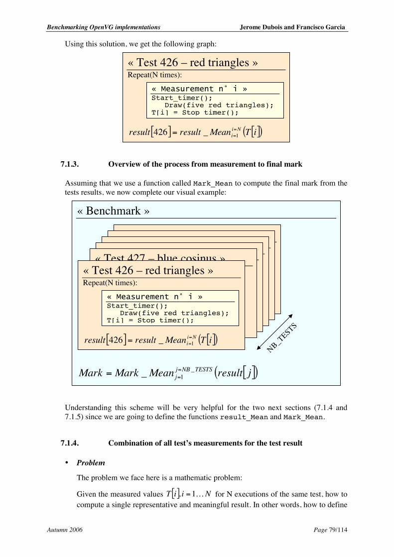
Benchmarking OpenVG implementations Jerome Dubois and Francisco Garcia
Autumn 2006 Page 79/114
Using this solution, we get the following graph:
7.1.3. Overview of the process from measurement to final mark
Assuming that we use a function called Mark_Mean to compute the final mark from the tests results, we now complete our visual example:
Understanding this scheme will be very helpful for the two next sections (7.1.4 and 7.1.5) since we are going to define the functions result_Mean and Mark_Mean.
7.1.4. Combination of all test’s measurements for the test result
• Problem
The problem we face here is a mathematic problem:
Given the measured values [ ] NiiT 1, = for N executions of the same test, how to compute a single representative and meaningful result. In other words, how to define
« Test 426 – red triangles » Repeat(N times):
[ ] [ ]( )iTMeanresultresult Nii=== 1_426
Start_timer(); Draw(five red triangles); T[i] = Stop_timer();
« Benchmark »
[ ]( )jresultMeanMarkMark TESTSNBjj
_1_ ===
« Test 427 – blue cosinus »
« Test 426 – red triangles » Repeat(N times):
[ ] [ ]( )iTMeanresultresult Nii=== 1_426
Start_timer(); Draw(five red triangles); T[i] = Stop_timer();
NB_TESTS
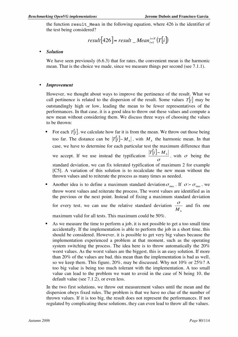
Benchmarking OpenVG implementations Jerome Dubois and Francisco Garcia
Autumn 2006 Page 80/114
the function result_Mean in the following equation, where 426 is the identifier of the test being considered?
[ ] [ ]( )iTMeanresultresult Nii=== 1_426
• Solution
We have seen previously (6.6.3) that for rates, the convenient mean is the harmonic mean. That is the choice we made, since we measure things per second (see 7.1.1).
• Improvement
However, we thought about ways to improve the pertinence of the result. What we call pertinence is related to the dispersion of the result. Some values [ ]iT may be outstandingly high or low, leading the mean to be fewer representatives of the performances. In that case, it is a good idea to throw out these values and compute a new mean without considering them. We discuss three ways of choosing the values to be thrown:
! For each [ ]iT , we calculate how far it is from the mean. We throw out those being too far. The distance can be [ ] hMiT − , with hM the harmonic mean. In that case, we have to determine for each particular test the maximum difference than
we accept. If we use instead the typification [ ]σ
hMiT −, with σ being the
standard deviation, we can fix tolerated typification of maximum 2 for example [C5]. A variation of this solution is to recalculate the new mean without the thrown values and to reiterate the process as many times as needed.
! Another idea is to define a maximum standard deviation maxσ . If maxσσ , we throw worst values and reiterate the process. The worst values are identified as in the previous or the next point. Instead of fixing a maximum standard deviation
for every test, we can use the relative standard deviation hM
σ and fix one
maximum valid for all tests. This maximum could be 50%. ! As we measure the time to perform a job, it is not possible to get a too small time
accidentally. If the implementation is able to perform the job in a short time, this should be considered. However, it is possible to get very big values because the implementation experienced a problem at that moment, such as the operating system switching the process. The idea here is to throw automatically the 20% worst values. As the worst values are the biggest, this is an easy solution. If more than 20% of the values are bad, this mean than the implementation is bad as well, so we keep them. This figure, 20%, may be discussed. Why not 10% or 25%? A too big value is being too much tolerant with the implementation. A too small value can lead to the problem we want to avoid in the case of N being 10, the default value (see 7.1.2), or even less.
In the two first solutions, we throw out measurement values until the mean and the dispersion obeys fixed rules. The problem is that we have no clue of the number of thrown values. If it is too big, the result does not represent the performances. If not regulated by complicating these solutions, they can even lead to throw all the values.
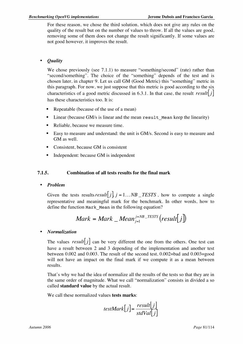
Benchmarking OpenVG implementations Jerome Dubois and Francisco Garcia
Autumn 2006 Page 81/114
For these reason, we chose the third solution, which does not give any rules on the quality of the result but on the number of values to throw. If all the values are good, removing some of them does not change the result significantly. If some values are not good however, it improves the result.
• Quality
We chose previously (see 7.1.1) to measure “something/second” (rate) rather than “second/something”. The choice of the “something” depends of the test and is chosen later, in chapter 9. Let us call GM (Good Metric) this “something” metric in this paragraph. For now, we just suppose that this metric is good according to the six characteristics of a good metric discussed in 6.3.1. In that case, the result [ ]jresult has these characteristics too. It is:
! Repeatable (because of the use of a mean) ! Linear (because GM/s is linear and the mean result_Mean keep the linearity) ! Reliable, because we measure time. ! Easy to measure and understand: the unit is GM/s. Second is easy to measure and
GM as well. ! Consistent, because GM is consistent ! Independent: because GM is independent
7.1.5. Combination of all tests results for the final mark
• Problem
Given the tests results [ ] TESTSNBjjresult _1, = , how to compute a single representative and meaningful mark for the benchmark. In other words, how to define the function Mark_Mean in the following equation?
[ ]( )jresultMeanMarkMark TESTSNBjj
_1_ ===
• Normalization
The values [ ]jresult can be very different the one from the others. One test can have a result between 2 and 3 depending of the implementation and another test between 0.002 and 0.003. The result of the second test, 0.002=bad and 0.003=good will not have an impact on the final mark if we compute it as a mean between results.
That’s why we had the idea of normalize all the results of the tests so that they are in the same order of magnitude. What we call “normalization” consists in divided a so called standard value by the actual result.
We call these normalized values tests marks:
[ ] [ ][ ]jstdValjresultjtestMark =
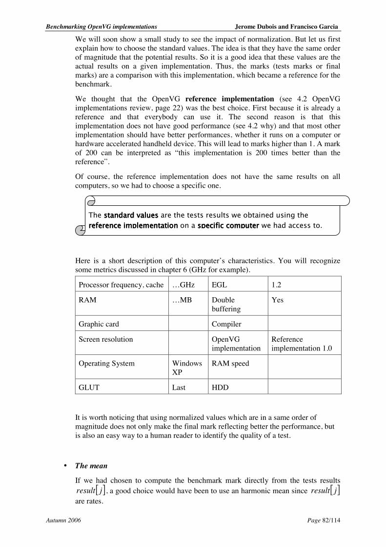
Benchmarking OpenVG implementations Jerome Dubois and Francisco Garcia
Autumn 2006 Page 82/114
We will soon show a small study to see the impact of normalization. But let us first explain how to choose the standard values. The idea is that they have the same order of magnitude that the potential results. So it is a good idea that these values are the actual results on a given implementation. Thus, the marks (tests marks or final marks) are a comparison with this implementation, which became a reference for the benchmark.
We thought that the OpenVG reference implementation (see 4.2 OpenVG implementations review, page 22) was the best choice. First because it is already a reference and that everybody can use it. The second reason is that this implementation does not have good performance (see 4.2 why) and that most other implementation should have better performances, whether it runs on a computer or hardware accelerated handheld device. This will lead to marks higher than 1. A mark of 200 can be interpreted as “this implementation is 200 times better than the reference”.
Of course, the reference implementation does not have the same results on all computers, so we had to choose a specific one.
Here is a short description of this computer’s characteristics. You will recognize some metrics discussed in chapter 6 (GHz for example).
Processor frequency, cache …GHz EGL 1.2
RAM …MB Double buffering
Yes
Graphic card Compiler
Screen resolution OpenVG implementation
Reference implementation 1.0
Operating System Windows XP
RAM speed
GLUT Last HDD
It is worth noticing that using normalized values which are in a same order of magnitude does not only make the final mark reflecting better the performance, but is also an easy way to a human reader to identify the quality of a test.
• The mean
If we had chosen to compute the benchmark mark directly from the tests results [ ]jresult , a good choice would have been to use an harmonic mean since [ ]jresult
are rates.
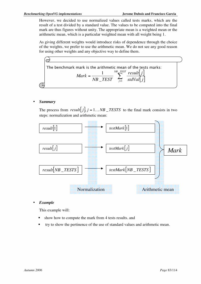
Benchmarking OpenVG implementations Jerome Dubois and Francisco Garcia
Autumn 2006 Page 83/114
However, we decided to use normalized values called tests marks, which are the result of a test divided by a standard value. The values to be computed into the final mark are thus figures without unity. The appropriate mean is a weighted mean or the arithmetic mean, which is a particular weighted mean with all weight being 1.
As giving different weights would introduce risks of dependence through the choice of the weights, we prefer to use the arithmetic mean. We do not see any good reason for using other weights and any objective way to define them.
• Summary
The process from [ ] TESTSNBjjresult _1, = to the final mark consists in two steps: normalization and arithmetic mean:
• Example
This example will:
! show how to compute the mark from 4 tests results, and ! try to show the pertinence of the use of standard values and arithmetic mean.
[ ]jresult
[ ]1result
[ ]TESTSNBresult _
[ ]1testMark
[ ]jtestMark
[ ]TESTSNBtestMark _
Mark
Normalization Arithmetic mean
[ ][ ]
=
=TESTNB
j jstdValjresult
TESTNBMark
_
1_1
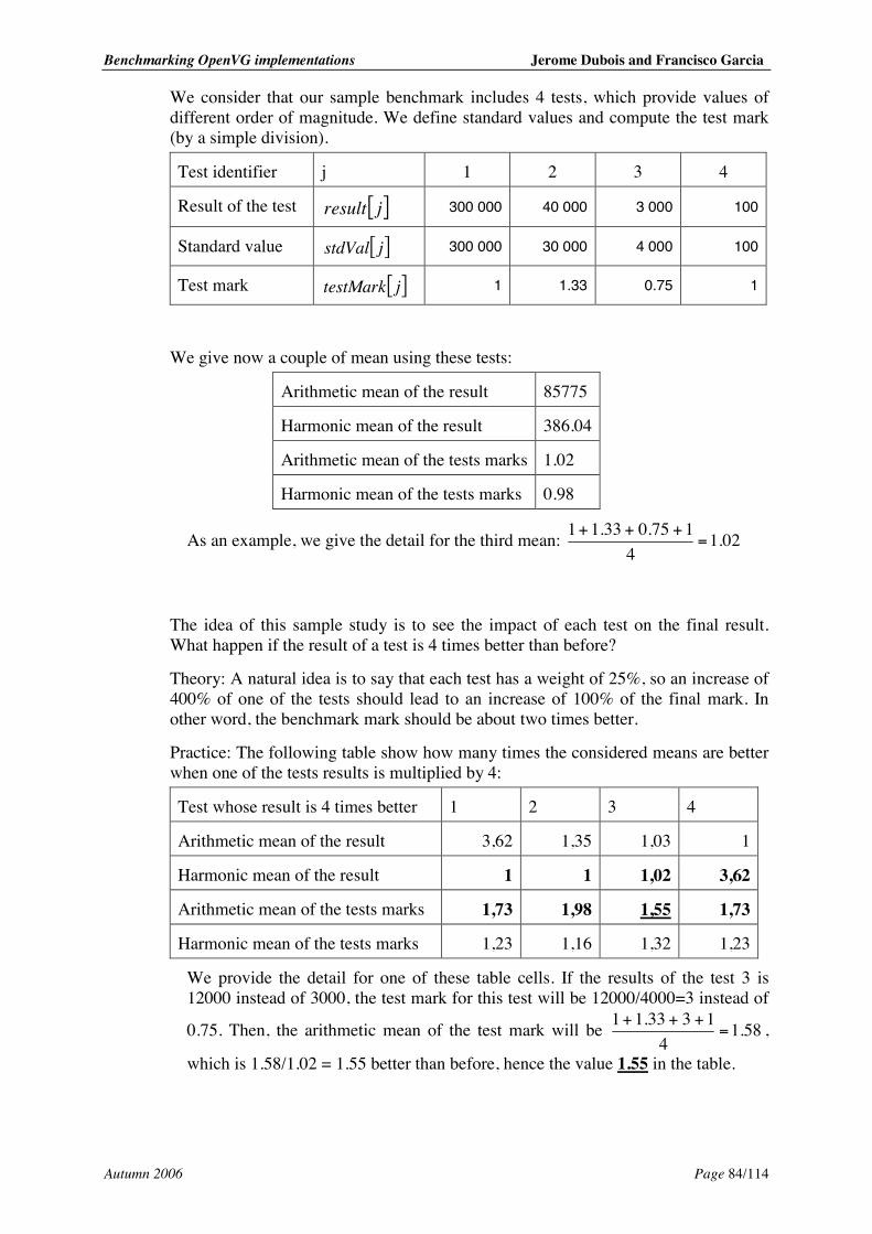
Benchmarking OpenVG implementations Jerome Dubois and Francisco Garcia
Autumn 2006 Page 84/114
We consider that our sample benchmark includes 4 tests, which provide values of different order of magnitude. We define standard values and compute the test mark (by a simple division).
Test identifier j 1 2 3 4
Result of the test [ ]jresult 300 000 40 000 3 000 100
Standard value [ ]jstdVal 300 000 30 000 4 000 100
Test mark [ ]jtestMark 1 1.33 0.75 1
We give now a couple of mean using these tests:
Arithmetic mean of the result 85775
Harmonic mean of the result 386.04
Arithmetic mean of the tests marks 1.02
Harmonic mean of the tests marks 0.98
As an example, we give the detail for the third mean: 02.14
175.033.11=
+++
The idea of this sample study is to see the impact of each test on the final result. What happen if the result of a test is 4 times better than before?
Theory: A natural idea is to say that each test has a weight of 25%, so an increase of 400% of one of the tests should lead to an increase of 100% of the final mark. In other word, the benchmark mark should be about two times better.
Practice: The following table show how many times the considered means are better when one of the tests results is multiplied by 4:
Test whose result is 4 times better 1 2 3 4
Arithmetic mean of the result 3,62 1,35 1,03 1
Harmonic mean of the result 1 1 1,02 3,62
Arithmetic mean of the tests marks 1,73 1,98 1,55 1,73
Harmonic mean of the tests marks 1,23 1,16 1,32 1,23
We provide the detail for one of these table cells. If the results of the test 3 is 12000 instead of 3000, the test mark for this test will be 12000/4000=3 instead of
0.75. Then, the arithmetic mean of the test mark will be 58.14
1333.11=
+++ ,
which is 1.58/1.02 = 1.55 better than before, hence the value 1.55 in the table.
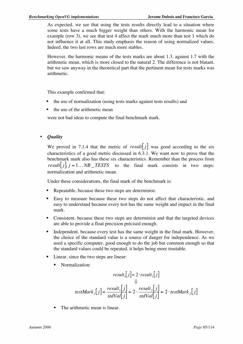
Benchmarking OpenVG implementations Jerome Dubois and Francisco Garcia
Autumn 2006 Page 85/114
As expected, we see that using the tests results directly lead to a situation where some tests have a much bigger weight than others. With the harmonic mean for example (row 3), we see that test 4 affect the mark much more than test 1 which do not influence it at all. This study emphasis the reason of using normalized values. Indeed, the two last rows are much more stables.
However, the harmonic means of the tests marks are about 1.3, against 1.7 with the arithmetic mean, which is more closed to the natural 2. The difference is not blatant, but we saw anyway in the theoretical part that the pertinent mean for tests marks was arithmetic.
This example confirmed that:
! the use of normalization (using tests marks against tests results) and ! the use of the arithmetic mean were not bad ideas to compute the final benchmark mark.
• Quality
We proved in 7.1.4 that the metric of [ ]jresult was good according to the six characteristics of a good metric discussed in 6.3.1. We want now to prove that the benchmark mark also has these six characteristics. Remember than the process from
[ ] TESTSNBjjresult _1, = to the final mark consists in two steps: normalization and arithmetic mean.
Under these considerations, the final mark of the benchmark is:
! Repeatable, because these two steps are determinist. ! Easy to measure because these two steps do not affect that characteristic, and
easy to understand because every test has the same weight and impact in the final mark.
! Consistent, because these two steps are determinist and that the targeted devices are able to provide a float precision précised enough.
! Independent, because every test has the same weight in the final mark. However, the choice of the standard value is a source of danger for independence. As we used a specific computer, good enough to do the job but common enough so that the standard values could be repeated, it helps being more trustable.
! Linear, since the two steps are linear: ! Normalization:
[ ] [ ]jresultjresult 21 2 ⋅=
[ ] [ ][ ]
[ ][ ]
[ ]jtestMarkjstdValjresult
jstdValjresult
jtestMark 221
1 22 ⋅=⋅==
! The arithmetic mean is linear.
Benchmarking OpenVG implementations Jerome Dubois and Francisco Garcia
Autumn 2006 Page 86/114
! Reliable. It is unfortunately not possible to prove the reliability by the theory. The benchmark should be tested to know if it is linear. However, the fact that each test has a similar impact into the final mark and the distribution of the tests in OpenVG functionality (see later) should help for the reliability.
7.2. PORTABILITY ISSUES
The aim of a benchmark is to run under several systems to make comparisons. Thus it should be easy to execute it easily on every system. Since OpenVG is intended to be used with different devices and operating systems, our benchmark has to be portable. A mobile phone has a small memory compared to a PC. Special cares should be taken.
The targeted devices and OpenVG implementations have different drawing surface size, to which our benchmark should adapt. A good idea is to give the size of the screen as a parameter of the benchmark.
An OpenVG benchmark is unfortunately platform dependant, because it has to set up the OpenVG implementation and environment. Our benchmark will fit the reference implementation, run on a windows platform and use GLUT and EGL, using double buffering.
To run on another platform, the code has to be adapted. This should not be very difficult since we have tried to separate the platform dependant code from the rest of the code.
The Makefile also need to be adapted to link with the suitable libraries (OpenVG, EGL, and others).
See the readme file for guidelines of how to port the benchmark.
7.3. OUTPUT OF THE BENCHMARK
7.3.1. Choice of the information for the output
We have explain in detail in this report why and how to compute a single mark for the benchmark. This is nice for people who are on a hurry and want an estimation of global performances. A benchmark should also be able to give more detailed results. This section presents the information that will be outputted in the most detailed output form. The benchmark user might want details of execution for every test, in order to identify strengths and weaknesses of the implementation. Finally, our benchmark outputs for each test: ! An identifier j for the test. This ID is an integer and is always the same for a test.
This permits to compare this specific test while changing a parameter or the OpenVG implementation.
! A description of the test.
! The test mark [ ] [ ] [ ]jstdValjresultjtestMark = .
! The test result [ ]jresult .
Benchmarking OpenVG implementations Jerome Dubois and Francisco Garcia
Autumn 2006 Page 87/114
! The standard value [ ]jstdVal .
! The unity in which the result is given (e.g.: shapes/second)
! The standard deviation [ ]jσ of the test.
! The coefficient of variation: [ ] [ ]jresultjσ This concept could be called “pertinence of the test”, since it gives an idea of the dispersion of the measurements actually considered, but in a normalized way, which allows comparing the pertinence of a set of tests and identifying tests whose dispersion is high. A high dispersion can indicate that the result of this test should not be trusted. It can also point out that the implementation is not consistent while performing this test.
! Possibly a warning, for example if this normalized deviation exceeds a fix limit. Additionally to the tests, some global variables should be outputted too: ! Parameters (screen size, repetition …), so that the results can be analyzed even
many time after the execution, for example if they were stored in a file. ! The number of values used for computing each result (20% of the repetition
number). ! A global consistency indicator: the arithmetic mean of the relative standard
deviation of each test results. ! An indicator of the performance distribution: the relative standard deviation of the
final Mark. ! Number of tests ! Total time of execution ! The final Mark
7.3.2. Output format
• Standard output
The main output is done on a console (shell), not on the device screen. It is done easily by the use of printf() on stdout actually.
There are three levels of detail for the output. The requested detail level is passed as a parameter to the benchmark. High detail levels include lowers.
! Level 3: The most detailed level. For each test executed, print on one line the information describe above in the first list of previous section (7.3.1)
! Level 2: Intermediate level. Print the global information about the execution, as describe above in the second list of previous section (7.3.1).
! Level 1: Print only the final Mark.
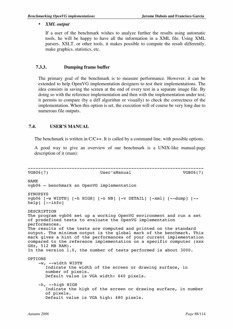
Benchmarking OpenVG implementations Jerome Dubois and Francisco Garcia
Autumn 2006 Page 88/114
• XML output
If a user of the benchmark wishes to analyze further the results using automatic tools, he will be happy to have all the information in a XML file. Using XML parsers, XSLT, or other tools, it makes possible to compute the result differently, make graphics, statistics, etc.
7.3.3. Dumping frame buffer
The primary goal of the benchmark is to measure performance. However, it can be extended to help OpenVG implementation designers to test their implementations. The idea consists in saving the screen at the end of every test in a separate image file. By doing so with the reference implementation and then with the implementation under test, it permits to compare (by a diff algorithm or visually) to check the correctness of the implementation. When this option is set, the execution will of course be very long due to numerous file outputs.
7.4. USER’S MANUAL
The benchmark is written in C/C++. It is called by a command line, with possible options.
A good way to give an overview of our benchmark is a UNIX-like manual-page description of it (man):
-------------------------------------------------------------------- VGB06(7) User’sManual VGB06(7) NAME vgb06 – benchmark an OpenVG implementation SYNOPSYS vgb06 [-w WIDTH] [-h HIGH] [-n NB] [-v DETAIL] [-xml] [--dump] [--help] [--info] DESCRIPTION The program vgb06 set up a working OpenVG environment and run a set of predefined tests to evaluate the OpenVG implementation performances. The results of the tests are computed and printed on the standard output. The minimum output is the global mark of the benchmark. This mark gives a hint of the performances of your current implementation compared to the reference implementation on a specific computer (xxx GHz, 512 MB RAM). In the version 1.0, the number of tests performed is about 3000. OPTIONS
-w, --width WIDTH Indicate the width of the screen or drawing surface, in number of pixels. Default value is VGA width: 640 pixels.
-h, --high HIGH
Indicate the high of the screen or drawing surface, in number of pixels. Default value is VGA high: 480 pixels.
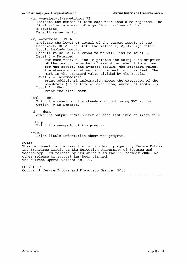
Benchmarking OpenVG implementations Jerome Dubois and Francisco Garcia
Autumn 2006 Page 89/114
-n, --number-of-repetition NB Indicate the number of time each test should be repeated. The final value is a mean of significant values of the executions. Default value is 10.
-v, --verbose DETAIL
Indicate the level of detail of the output result of the benchmark. DETAIL can take the values 1, 2, 3. High detail levels include lowers. Default value is 1. A wrong value will lead to level 3. Level 3 – Detailed
For each test, a line is printed including a description of the test, the number of execution taken into account for the result, the average result, the standard value, the standard deviation, and the mark for this test. The mark is the standard value divided by the result.
Level 2 – Intermediate Print additional information about the execution of the benchmark (total time of execution, number of tests...)
Level 1 – Short Print the final mark.
-xml, --xml
Print the result on the standard output using XML syntax. Option -v is ignored.
-d, --dump
dump the output frame buffer of each test into an image file. --help
Print the synopsis of the program. --info
Print little information about the program. NOTES This benchmark is the result of an academic project by Jerome Dubois and Francisco Garcia at the Norwegian University of Science and Technology. Its release by its authors is the 22 December 2006. No other release or support has been planned. The current OpenVG version is 1.0. COPYRIGHT Copyright Jerome Dubois and Francisco Garcia, 2006 --------------------------------------------------------------------
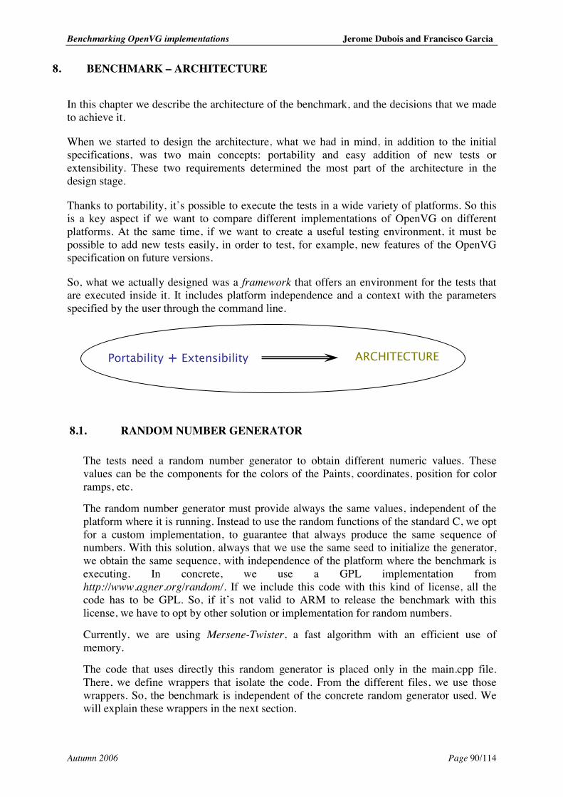
Benchmarking OpenVG implementations Jerome Dubois and Francisco Garcia
Autumn 2006 Page 90/114
8. BENCHMARK – ARCHITECTURE
In this chapter we describe the architecture of the benchmark, and the decisions that we made to achieve it.
When we started to design the architecture, what we had in mind, in addition to the initial specifications, was two main concepts: portability and easy addition of new tests or extensibility. These two requirements determined the most part of the architecture in the design stage.
Thanks to portability, it’s possible to execute the tests in a wide variety of platforms. So this is a key aspect if we want to compare different implementations of OpenVG on different platforms. At the same time, if we want to create a useful testing environment, it must be possible to add new tests easily, in order to test, for example, new features of the OpenVG specification on future versions.
So, what we actually designed was a framework that offers an environment for the tests that are executed inside it. It includes platform independence and a context with the parameters specified by the user through the command line.
8.1. RANDOM NUMBER GENERATOR
The tests need a random number generator to obtain different numeric values. These values can be the components for the colors of the Paints, coordinates, position for color ramps, etc.
The random number generator must provide always the same values, independent of the platform where it is running. Instead to use the random functions of the standard C, we opt for a custom implementation, to guarantee that always produce the same sequence of numbers. With this solution, always that we use the same seed to initialize the generator, we obtain the same sequence, with independence of the platform where the benchmark is executing. In concrete, we use a GPL implementation from http://www.agner.org/random/. If we include this code with this kind of license, all the code has to be GPL. So, if it’s not valid to ARM to release the benchmark with this license, we have to opt by other solution or implementation for random numbers.
Currently, we are using Mersene-Twister, a fast algorithm with an efficient use of memory.
The code that uses directly this random generator is placed only in the main.cpp file. There, we define wrappers that isolate the code. From the different files, we use those wrappers. So, the benchmark is independent of the concrete random generator used. We will explain these wrappers in the next section.
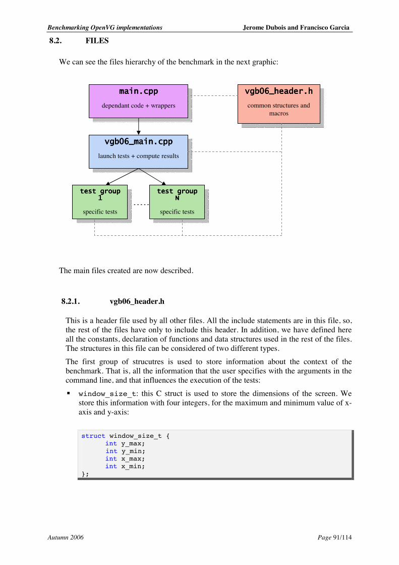
Benchmarking OpenVG implementations Jerome Dubois and Francisco Garcia
Autumn 2006 Page 91/114
8.2. FILES
We can see the files hierarchy of the benchmark in the next graphic:
The main files created are now described.
8.2.1. vgb06_header.h
This is a header file used by all other files. All the include statements are in this file, so, the rest of the files have only to include this header. In addition, we have defined here all the constants, declaration of functions and data structures used in the rest of the files. The structures in this file can be considered of two different types. The first group of strucutres is used to store information about the context of the benchmark. That is, all the information that the user specifies with the arguments in the command line, and that influences the execution of the tests: ! window_size_t: this C struct is used to store the dimensions of the screen. We
store this information with four integers, for the maximum and minimum value of x-axis and y-axis:
struct window_size_t { int y_max; int y_min; int x_max; int x_min; };
.....
dependant code + wrappers
launch tests + compute results
specific tests
specific tests
common structures and macros
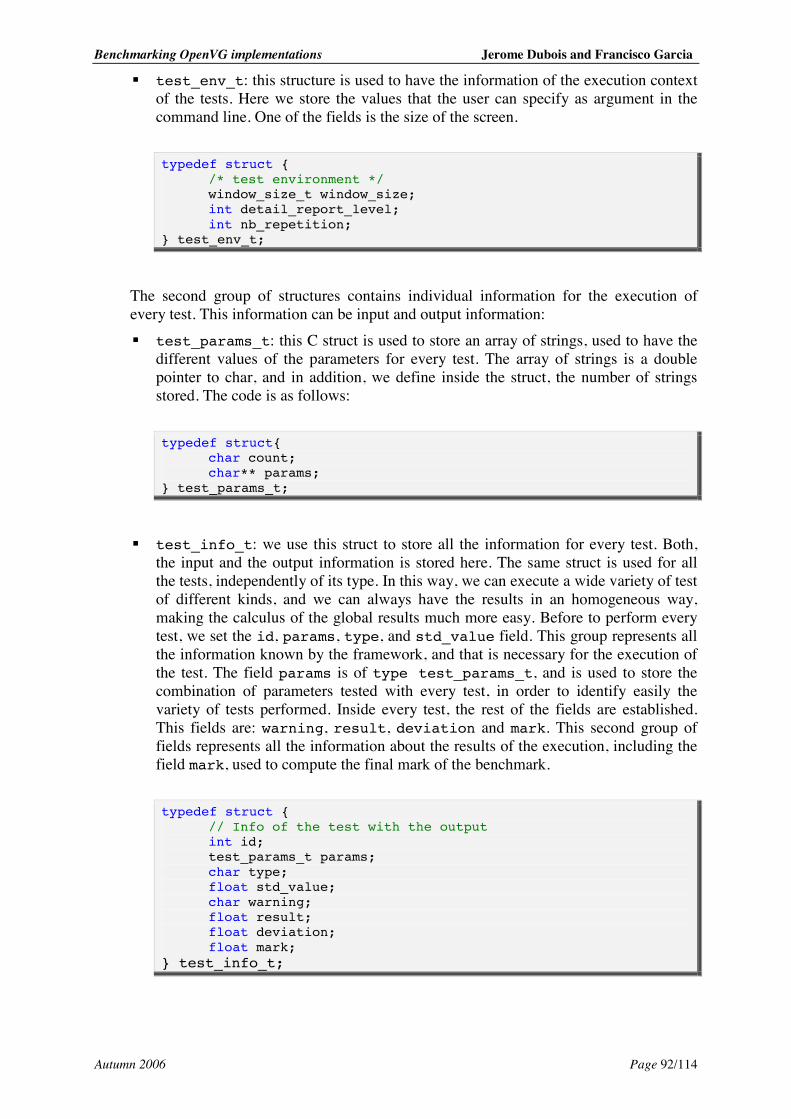
Benchmarking OpenVG implementations Jerome Dubois and Francisco Garcia
Autumn 2006 Page 92/114
! test_env_t: this structure is used to have the information of the execution context of the tests. Here we store the values that the user can specify as argument in the command line. One of the fields is the size of the screen.
typedef struct { /* test environment */ window_size_t window_size; int detail_report_level; int nb_repetition; } test_env_t;
The second group of structures contains individual information for the execution of every test. This information can be input and output information: ! test_params_t: this C struct is used to store an array of strings, used to have the
different values of the parameters for every test. The array of strings is a double pointer to char, and in addition, we define inside the struct, the number of strings stored. The code is as follows:
typedef struct{ char count; char** params; } test_params_t;
! test_info_t: we use this struct to store all the information for every test. Both,
the input and the output information is stored here. The same struct is used for all the tests, independently of its type. In this way, we can execute a wide variety of test of different kinds, and we can always have the results in an homogeneous way, making the calculus of the global results much more easy. Before to perform every test, we set the id, params, type, and std_value field. This group represents all the information known by the framework, and that is necessary for the execution of the test. The field params is of type test_params_t, and is used to store the combination of parameters tested with every test, in order to identify easily the variety of tests performed. Inside every test, the rest of the fields are established. This fields are: warning, result, deviation and mark. This second group of fields represents all the information about the results of the execution, including the field mark, used to compute the final mark of the benchmark.
typedef struct { // Info of the test with the output int id; test_params_t params; char type; float std_value; char warning; float result; float deviation; float mark; } test_info_t;
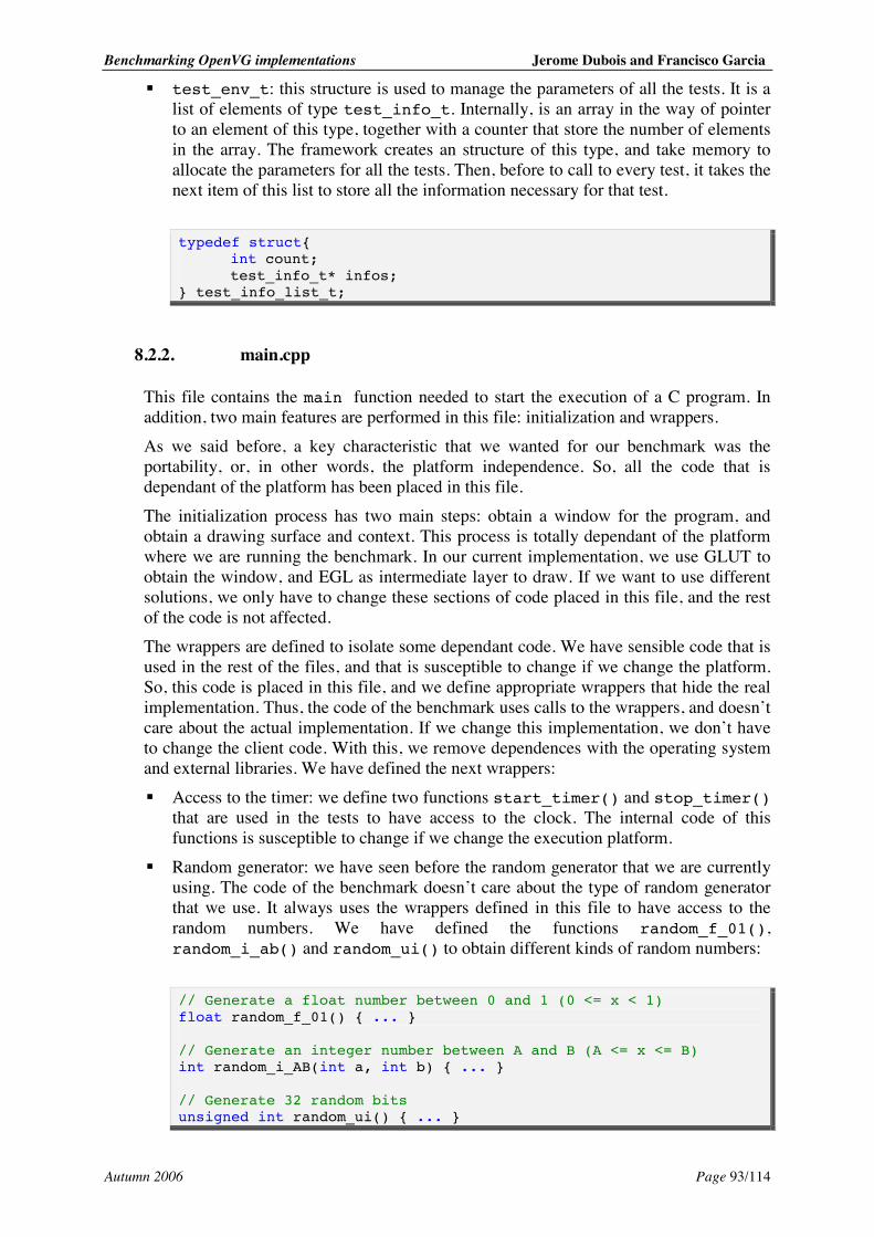
Benchmarking OpenVG implementations Jerome Dubois and Francisco Garcia
Autumn 2006 Page 93/114
! test_env_t: this structure is used to manage the parameters of all the tests. It is a list of elements of type test_info_t. Internally, is an array in the way of pointer to an element of this type, together with a counter that store the number of elements in the array. The framework creates an structure of this type, and take memory to allocate the parameters for all the tests. Then, before to call to every test, it takes the next item of this list to store all the information necessary for that test.
typedef struct{ int count; test_info_t* infos; } test_info_list_t;
8.2.2. main.cpp
This file contains the main function needed to start the execution of a C program. In addition, two main features are performed in this file: initialization and wrappers. As we said before, a key characteristic that we wanted for our benchmark was the portability, or, in other words, the platform independence. So, all the code that is dependant of the platform has been placed in this file. The initialization process has two main steps: obtain a window for the program, and obtain a drawing surface and context. This process is totally dependant of the platform where we are running the benchmark. In our current implementation, we use GLUT to obtain the window, and EGL as intermediate layer to draw. If we want to use different solutions, we only have to change these sections of code placed in this file, and the rest of the code is not affected. The wrappers are defined to isolate some dependant code. We have sensible code that is used in the rest of the files, and that is susceptible to change if we change the platform. So, this code is placed in this file, and we define appropriate wrappers that hide the real implementation. Thus, the code of the benchmark uses calls to the wrappers, and doesn’t care about the actual implementation. If we change this implementation, we don’t have to change the client code. With this, we remove dependences with the operating system and external libraries. We have defined the next wrappers: ! Access to the timer: we define two functions start_timer() and stop_timer()
that are used in the tests to have access to the clock. The internal code of this functions is susceptible to change if we change the execution platform.
! Random generator: we have seen before the random generator that we are currently using. The code of the benchmark doesn’t care about the type of random generator that we use. It always uses the wrappers defined in this file to have access to the random numbers. We have defined the functions random_f_01(), random_i_ab() and random_ui() to obtain different kinds of random numbers:
// Generate a float number between 0 and 1 (0 <= x < 1) float random_f_01() { ... } // Generate an integer number between A and B (A <= x <= B) int random_i_AB(int a, int b) { ... } // Generate 32 random bits unsigned int random_ui() { ... }
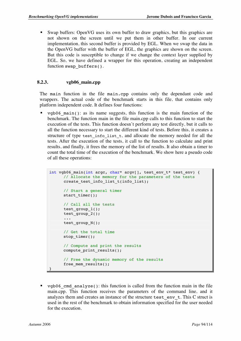
Benchmarking OpenVG implementations Jerome Dubois and Francisco Garcia
Autumn 2006 Page 94/114
! Swap buffers: OpenVG uses its own buffer to draw graphics, but this graphics are
not shown on the screen until we put them in other buffer. In our current implementation, this second buffer is provided by EGL. When we swap the data in the OpenVG buffer with the buffer of EGL, the graphics are shown on the screen. But this code is susceptible to change if we change the context layer supplied by EGL. So, we have defined a wrapper for this operation, creating an independent function swap_buffers().
8.2.3. vgb06_main.cpp
The main function in the file main.cpp contains only the dependant code and wrappers. The actual code of the benchmark starts in this file, that contains only platform independent code. It defines four functions: ! vgb06_main(): as its name suggests, this function is the main function of the
benchmark. The function main in the file main.cpp calls to this function to start the execution of the tests. This function doesn’t perform any test directly, but it calls to all the function necessary to start the different kind of tests. Before this, it creates a structure of type test_info_list_t, and allocate the memory needed for all the tests. After the execution of the tests, it call to the function to calculate and print results, and finally, it frees the memory of the list of results. It also obtain a timer to count the total time of the execution of the benchmark. We show here a pseudo code of all these operations:
int vgb06_main(int argc, char* argv[], test_env_t* test_env) { // Allocate the memory for the parameters of the tests create_test_info_list_t(info_list); // Start a general timer start_timer(); // Call all the tests test_group_1(); test_group_2(); ... test_group_N(); // Get the total time stop_timer(); // Compute and print the results compute_print_results(); // Free the dynamic memory of the results free_mem_results(); }
! vgb06_cmd_analyze(): this function is called from the function main in the file
main.cpp. This function receives the parameters of the command line, and it analyzes them and creates an instance of the structure test_env_t. This C struct is used in the rest of the benchmark to obtain information specified for the user needed for the execution.
Benchmarking OpenVG implementations Jerome Dubois and Francisco Garcia
Autumn 2006 Page 95/114
void vgb06_cmd_analyze(int argc, char* argv[], test_env_t *test_env) { ... }
! free_mem_results(): the benchmark is going to be used, mainly, in handheld
devices with a reduced quantity of memory. So, it is very important to free all the resources used by the benchmark. In this function, we free the dynamic memory used to allocate the input and output parameters of the tests.
void free_mem_results(test_info_list_t *info_list) { ... }
! compute_print_results(): this function receive the list of results of the tests,
with the individual marks, and compute the final mark of the benchmark. In addition, it prints the results on the screen.
void compute_print_results(test_info_list_t *info_list, long total_time, int detail_level) { ... }
! print_xml(): this function receives the list of results of the tests, and print the
result in XML format. With this, it is possible to use external tools to analyze the data of the benchmark, and it opens a wide set of possibilities.
void print_xml(test_info_list_t *info_list, long total_time, int detail_level) { ... }
8.2.4. Test files
Each individual test has a unique integer identifier, starting from 1 to NB_TESTS, and a test_info structure associated. The tests are organized in tests groups, and each of these groups try a different feature or group of related features of OpenVG. Each group of tests, has a main function that is the starting point of its execution, and performs the tasks to execute all the tests. The main function is called from vgb06_main(). As a convention, this functions should be called execute_xxx_tests(...), where xxx is a name for the tests group. They are given the test_info_list_t structure created in vgb06_main(), to store the info of every individual test. These execute_xxx_tests(...) functions call to every individual test, and at the end, the framework finds all the information in the list of results, used to compute the final results of the benchmark.
For example, the test number 843 will fill the test_info_list[843] structure.
Benchmarking OpenVG implementations Jerome Dubois and Francisco Garcia
Autumn 2006 Page 96/114
9. BENCHMARK – TEST DESIGN
Once we have a suitable framework, portable and extensible, we need to define a real valuable set of tests, which give information about the performance of the platform on the most important OpenVG features.
In this chapter we will show the process to identify and obtain this set of features to test.
9.1. CATEGORIES OF FEATURES
It is possible to identify six categories of OpenVG features:
! Paths features: these tests should involve a big number of OpenVG paths in order to obtain a degree of performance over this kind of operations.
! Paint features: tests with a few numbers of paths with big areas to paint. Thus, it is possible to test the Paint performance of the platform.
! Images features: tests involving image operations. ! VGU features: tests with the extensions to the OpenVG API. ! Other features dependant of Path, Paint and Images: some other features must by tested
using Paths, Paints and Images. This is the case of rendering quality, scissoring or masking. These tests should be done using these three kinds of objects in order to obtain real results about their performance.
! Other features independent of Path, Paint and Images: other features are independent of these main objects of OpenVG. This is the case of features like clearing, matrix manipulation and querying hardware capabilities.
It is obvious that to create a benchmark that tests all the categories shown above is a very complicated task. So, it is preferable to split these sets of functionalities and focus individually in some of them.
Thus, our work consisted on create a benchmark to test the paints features of OpenVG.
Graphic tests can be separated on two different types:
! Geometry tests: those which require a big quantity of geometry processing. What we measure is the processing performance. The appropriate metric is the number of primitive per second (lines for example). We call this kind as g-tests.
! Figurate tests: those which affect a big part of the screen. These tests should measure the colors, images and gradients processing performances. Appropriate metric is an approximation of the number of pixel affected divided by the performing time, pixels/second. We call this kind as f-tests.
Paint tests are inside the group of Figurate tests, so, the results of our tests should be in the form of pixels/second. This is an appropriate metric for this kind of benchmarking.
Benchmarking OpenVG implementations Jerome Dubois and Francisco Garcia
Autumn 2006 Page 97/114
9.2. IDENTIFYING APPROPRIATE PARAMETERS
We know now exactly which subset of the OpenVG API features we are going to focus on: Paints. Now, we need to identify the most important parameters inside this group. This is, what can we benchmark? The next step should be to give appropriate values to these identified parameters.
9.2.1. Parameter A: Opacity
We express the color for the Paints in RGBA mode. Before drawing the objects on the drawing surface, OpenVG has to calculate the exact value for the RGB channels. That is, it has to multiply every RGB value by the alpha value. This is a very basic characteristic, which is repeated so many times. So, we want to tests if the platform is affected by these calculations. Thus, we define two different values for this parameter: ! Opaque: with opaque color, the alpha value will be always equal to 1, and some
implementations could have this into account in order to be more efficient. ! Transparent: with transparent colors, the alpha value will be a value in [0,1].
9.2.2. Parameter B: Number of color stops
Inside linear and radial gradient, it is necessary to define a different number of color stops. On each stop, a different color is applied, according with the gradient function. So, it’s interesting to tests if a different number of color stops affects to the performance of the applications. In our tests, we have three different values for this parameter: 2, 5 and 10. Thus, we can check if this difference affects to the performance. This parameter has sense only with paint of type linear and radial. Color and pattern paints are not affected by this parameter.
9.2.3. Parameter C: Ramp spread mode
Spread modes define how the color stops are repeated when they finish. This parameter, equal than number of color stops, is applied only when linear and radial gradients are used. This is a parameter in the context of OpenVG. It is possible to assign three different values to it: ! Pad: this value extends the stops when they finish. ! Repeat: this option repeats indefinitely in both directions the sequence of stops
when they finish. ! Reflect: this value repeats in both directions indefinitely the sequence of stops in
inverse order when they finish. In our tests, we use these three values, in order to measure the performance with all the different combinations.
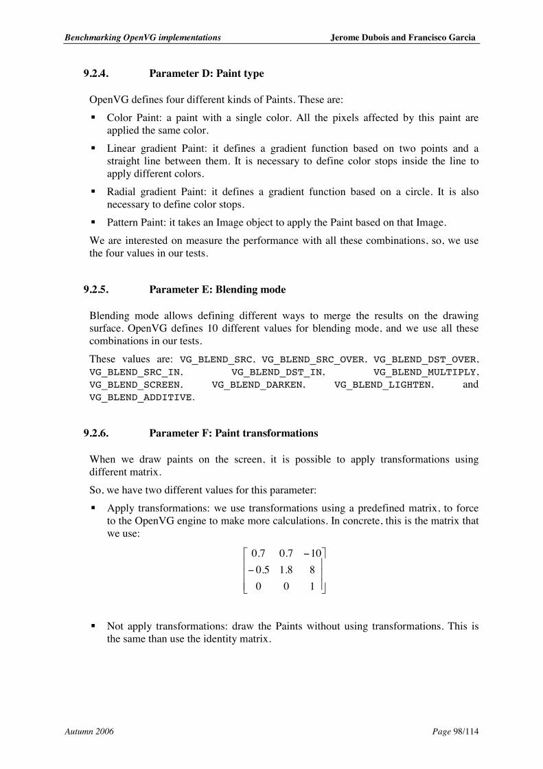
Benchmarking OpenVG implementations Jerome Dubois and Francisco Garcia
Autumn 2006 Page 98/114
9.2.4. Parameter D: Paint type
OpenVG defines four different kinds of Paints. These are: ! Color Paint: a paint with a single color. All the pixels affected by this paint are
applied the same color. ! Linear gradient Paint: it defines a gradient function based on two points and a
straight line between them. It is necessary to define color stops inside the line to apply different colors.
! Radial gradient Paint: it defines a gradient function based on a circle. It is also necessary to define color stops.
! Pattern Paint: it takes an Image object to apply the Paint based on that Image. We are interested on measure the performance with all these combinations, so, we use the four values in our tests.
9.2.5. Parameter E: Blending mode
Blending mode allows defining different ways to merge the results on the drawing surface. OpenVG defines 10 different values for blending mode, and we use all these combinations in our tests. These values are: VG_BLEND_SRC, VG_BLEND_SRC_OVER, VG_BLEND_DST_OVER, VG_BLEND_SRC_IN, VG_BLEND_DST_IN, VG_BLEND_MULTIPLY, VG_BLEND_SCREEN, VG_BLEND_DARKEN, VG_BLEND_LIGHTEN, and VG_BLEND_ADDITIVE.
9.2.6. Parameter F: Paint transformations
When we draw paints on the screen, it is possible to apply transformations using different matrix. So, we have two different values for this parameter: ! Apply transformations: we use transformations using a predefined matrix, to force
to the OpenVG engine to make more calculations. In concrete, this is the matrix that we use:
−
−
10088.15.0107.07.0
! Not apply transformations: draw the Paints without using transformations. This is
the same than use the identity matrix.
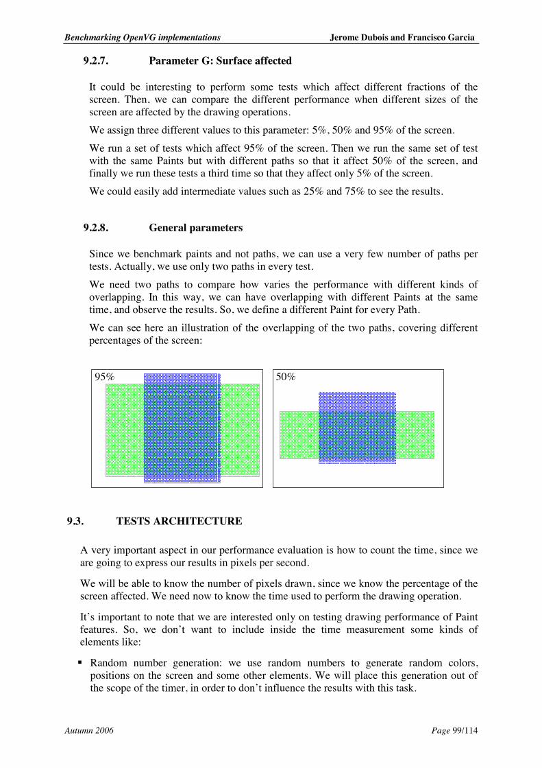
Benchmarking OpenVG implementations Jerome Dubois and Francisco Garcia
Autumn 2006 Page 99/114
9.2.7. Parameter G: Surface affected
It could be interesting to perform some tests which affect different fractions of the screen. Then, we can compare the different performance when different sizes of the screen are affected by the drawing operations. We assign three different values to this parameter: 5%, 50% and 95% of the screen. We run a set of tests which affect 95% of the screen. Then we run the same set of test with the same Paints but with different paths so that it affect 50% of the screen, and finally we run these tests a third time so that they affect only 5% of the screen. We could easily add intermediate values such as 25% and 75% to see the results.
9.2.8. General parameters
Since we benchmark paints and not paths, we can use a very few number of paths per tests. Actually, we use only two paths in every test. We need two paths to compare how varies the performance with different kinds of overlapping. In this way, we can have overlapping with different Paints at the same time, and observe the results. So, we define a different Paint for every Path. We can see here an illustration of the overlapping of the two paths, covering different percentages of the screen:
9.3. TESTS ARCHITECTURE
A very important aspect in our performance evaluation is how to count the time, since we are going to express our results in pixels per second.
We will be able to know the number of pixels drawn, since we know the percentage of the screen affected. We need now to know the time used to perform the drawing operation.
It’s important to note that we are interested only on testing drawing performance of Paint features. So, we don’t want to include inside the time measurement some kinds of elements like:
! Random number generation: we use random numbers to generate random colors, positions on the screen and some other elements. We will place this generation out of the scope of the timer, in order to don’t influence the results with this task.
95% 50%
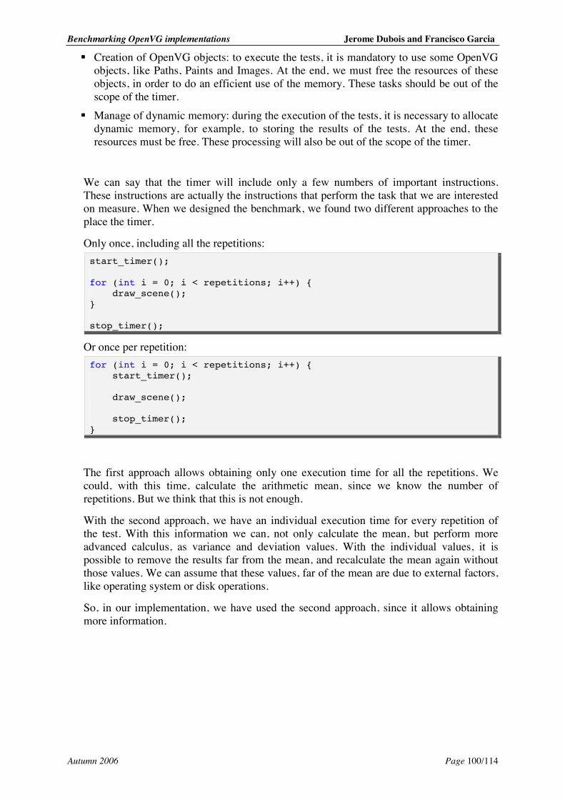
Benchmarking OpenVG implementations Jerome Dubois and Francisco Garcia
Autumn 2006 Page 100/114
! Creation of OpenVG objects: to execute the tests, it is mandatory to use some OpenVG objects, like Paths, Paints and Images. At the end, we must free the resources of these objects, in order to do an efficient use of the memory. These tasks should be out of the scope of the timer.
! Manage of dynamic memory: during the execution of the tests, it is necessary to allocate dynamic memory, for example, to storing the results of the tests. At the end, these resources must be free. These processing will also be out of the scope of the timer.
We can say that the timer will include only a few numbers of important instructions. These instructions are actually the instructions that perform the task that we are interested on measure. When we designed the benchmark, we found two different approaches to the place the timer.
Only once, including all the repetitions: start_timer(); for (int i = 0; i < repetitions; i++) { draw_scene(); } stop_timer();
Or once per repetition: for (int i = 0; i < repetitions; i++) { start_timer(); draw_scene(); stop_timer(); }
The first approach allows obtaining only one execution time for all the repetitions. We could, with this time, calculate the arithmetic mean, since we know the number of repetitions. But we think that this is not enough.
With the second approach, we have an individual execution time for every repetition of the test. With this information we can, not only calculate the mean, but perform more advanced calculus, as variance and deviation values. With the individual values, it is possible to remove the results far from the mean, and recalculate the mean again without those values. We can assume that these values, far of the mean are due to external factors, like operating system or disk operations.
So, in our implementation, we have used the second approach, since it allows obtaining more information.
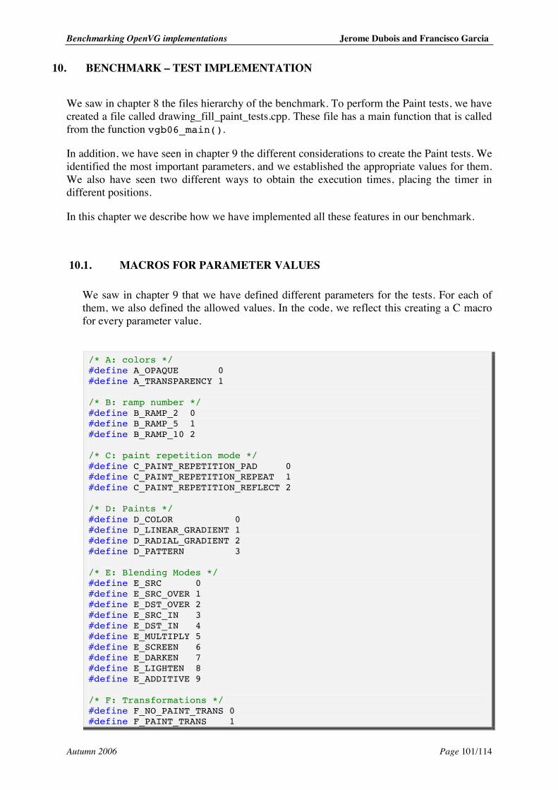
Benchmarking OpenVG implementations Jerome Dubois and Francisco Garcia
Autumn 2006 Page 101/114
10. BENCHMARK – TEST IMPLEMENTATION
We saw in chapter 8 the files hierarchy of the benchmark. To perform the Paint tests, we have created a file called drawing_fill_paint_tests.cpp. These file has a main function that is called from the function vgb06_main().
In addition, we have seen in chapter 9 the different considerations to create the Paint tests. We identified the most important parameters, and we established the appropriate values for them. We also have seen two different ways to obtain the execution times, placing the timer in different positions.
In this chapter we describe how we have implemented all these features in our benchmark.
10.1. MACROS FOR PARAMETER VALUES
We saw in chapter 9 that we have defined different parameters for the tests. For each of them, we also defined the allowed values. In the code, we reflect this creating a C macro for every parameter value.
/* A: colors */ #define A_OPAQUE 0 #define A_TRANSPARENCY 1 /* B: ramp number */ #define B_RAMP_2 0 #define B_RAMP_5 1 #define B_RAMP_10 2 /* C: paint repetition mode */ #define C_PAINT_REPETITION_PAD 0 #define C_PAINT_REPETITION_REPEAT 1 #define C_PAINT_REPETITION_REFLECT 2 /* D: Paints */ #define D_COLOR 0 #define D_LINEAR_GRADIENT 1 #define D_RADIAL_GRADIENT 2 #define D_PATTERN 3 /* E: Blending Modes */ #define E_SRC 0 #define E_SRC_OVER 1 #define E_DST_OVER 2 #define E_SRC_IN 3 #define E_DST_IN 4 #define E_MULTIPLY 5 #define E_SCREEN 6 #define E_DARKEN 7 #define E_LIGHTEN 8 #define E_ADDITIVE 9 /* F: Transformations */ #define F_NO_PAINT_TRANS 0 #define F_PAINT_TRANS 1
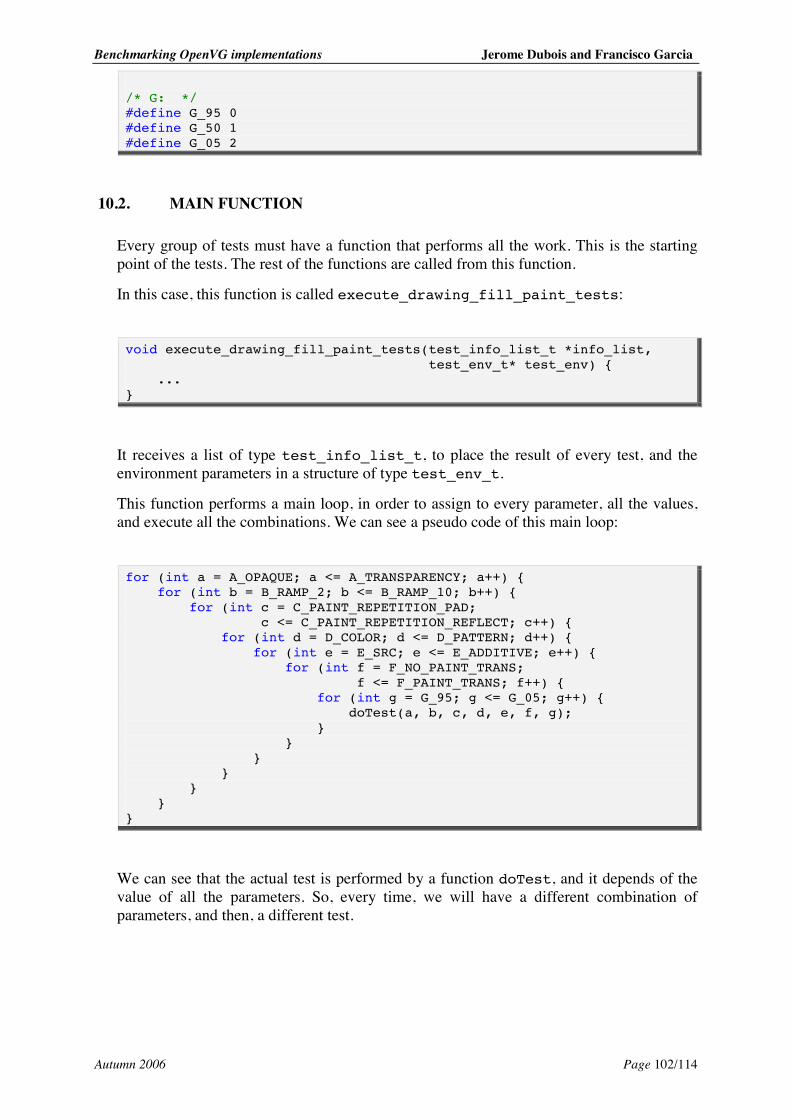
Benchmarking OpenVG implementations Jerome Dubois and Francisco Garcia
Autumn 2006 Page 102/114
/* G: */ #define G_95 0 #define G_50 1 #define G_05 2
10.2. MAIN FUNCTION
Every group of tests must have a function that performs all the work. This is the starting point of the tests. The rest of the functions are called from this function.
In this case, this function is called execute_drawing_fill_paint_tests:
void execute_drawing_fill_paint_tests(test_info_list_t *info_list, test_env_t* test_env) { ... }
It receives a list of type test_info_list_t, to place the result of every test, and the environment parameters in a structure of type test_env_t.
This function performs a main loop, in order to assign to every parameter, all the values, and execute all the combinations. We can see a pseudo code of this main loop:
for (int a = A_OPAQUE; a <= A_TRANSPARENCY; a++) { for (int b = B_RAMP_2; b <= B_RAMP_10; b++) { for (int c = C_PAINT_REPETITION_PAD; c <= C_PAINT_REPETITION_REFLECT; c++) { for (int d = D_COLOR; d <= D_PATTERN; d++) { for (int e = E_SRC; e <= E_ADDITIVE; e++) { for (int f = F_NO_PAINT_TRANS; f <= F_PAINT_TRANS; f++) { for (int g = G_95; g <= G_05; g++) { doTest(a, b, c, d, e, f, g); } } } } } } }
We can see that the actual test is performed by a function doTest, and it depends of the value of all the parameters. So, every time, we will have a different combination of parameters, and then, a different test.
Benchmarking OpenVG implementations Jerome Dubois and Francisco Garcia
Autumn 2006 Page 103/114
10.3. PATHS GENERATION
Every test will contain always two Paths. At the same time, we have defined three different sizes of Paths in the tests, to cover different percentage of the screen. So, we need six different Paths, which will be always the same ones. We create these six Paths out of the main loop and we store them in an array. In this way, we don’t have to recreate the same Paths more than once.
The function generatePaths create the six Paths, and store them in an array called path_array:
void generatePaths(test_env_t* test_env) { ... }
This function receives the environment parameters of the benchmark in order to adapt the sizes of the Paths to the actual size of the screen.
The function freePaths, is called at the end of the test group, and free the resources associated with the Paths, calling to the OpenVG function vgDestroyPath for every Path in path_array:
void freePaths(int nb_paths) { ... }
This function is independent of the number of Paths created with generatePaths, so it requires the number of Paths inside path_array.
Inside the main loop, one of the for statements, goes through the values of the parameter G, of affected surface. Inside this for, instead of creating a new two Paths for the next test, with the size needed, we only have to choose those Paths from path_array. This tasks is performed by the function choosePaths:
VGPath *choosePaths(int path_type) { ... }
It receives the value of parameter G, in order to choose the appropriate Paths of the array.
10.4. PAINT GENERATION
We assign a different Paint for every Path in every test. For each Paint we run the tests for the different Path sizes, different blending modes and transformations. So, we generate those Paints to reuse them in more than one test.
Benchmarking OpenVG implementations Jerome Dubois and Francisco Garcia
Autumn 2006 Page 104/114
The Paint generation is performed by the function generatPaints, and it stores the Paint objects in an array called paint_array: void generatePaints(int paint_type, int color_type, int ramp_number, int repetition_mode, int nb_paths, test_env_t* test_env) { ... }
It receives the value of the parameters that affect the Paint creation, that is, parameters A, B, C and D, and the environment parameters.
When we execute all the combinations for the generated Paints, we have to free their resources before to create a different set of Paints. This is done by the function freePaints: void freePaints(int nb_paths) { ... }
10.5. SETTING BLENDING MODES AND PAINT TRANSFORMATIONS
Parameters E and F are about blending modes and Paint transformations. For each value of these parameters, we have to set some parameters in the context of OpenVG before to execute the test.
Thus, with each different value of these parameters, we establish different values on the OpenVG context, and then, we obtain different test combinations.
To set in the context the values of blending mode, we have created the function setBlendingMode:
void setBlendingMode(int blending_type) { ... }
It receives as parameter, the value of the parameter E.
To set in the context the different Paint transformation values, the function setPaintTransformation has been created:
void setPaintTransformation(int transformation_type) { ... }
It receives the value of the parameter F, to set in the context the appropriate transformation.
Benchmarking OpenVG implementations Jerome Dubois and Francisco Garcia
Autumn 2006 Page 105/114
10.6. SKIPPING PARAMETER COMBINATIONS
Some combinations of parameters have no sense. For example, the number of color stops for color Paint or, patter Paint.
Inside the main loop, we have two places where we skip these kinds of combinations. With this, the code is more efficient.
The function skipPaintCombination skips the invalid combinations before to generate the Paints for the current combination of parameters:
char skipPaintCombination(int a, int b, int c, int d) { ... }
It receives parameters A, B, C and D, and returns a boolean value indicating if the current combination should be skipped.
The function skipTransformCombination skips the invalid combinations before to perform Paint transformations:
char skipTransformCombinations(int a, int b, int c, int d, int e, int f) { ... }
It receives parameters A, B, C, D, E, and F and returns with a Boolean value if the current combination is invalid or not.
10.7. PERFORMING THE TESTS
For every valid combination, we perform a test. This test is configured by the current values of each parameter. This is done by the function doTestFill:
void doTestFill(test_info_t* info, VGPath *paths_test, VGPaint *paint_array, int nb_paths, test_env_t* test_env) { ... }
When this function is called, some parameters are already established in the OpenVG context, and they will affect the drawing operations performed on this function. In addition, this function receives the Paths and Paint arrays, the parameters of the benchmark, and the structure of type test_info_t to place the results.
Benchmarking OpenVG implementations Jerome Dubois and Francisco Garcia
Autumn 2006 Page 106/114
The drawing operation will be executed the number of times specified by the user. In chapter 9, we saw two different ways to use the timer to execute the tests. The test are executed in this function, so the timer is placed here. We opt by the second option, in order to get the individual time for each repetition. With separate information, we can calculate more results.
These results are calculated in the function calculateTestResults, and it is called from doTestFill when all the repetitions of the test have finished and all the individual values have been collected in an array.
void calculateTestResults(test_info_t *info, unsigned long *individual_times, int repetitions) { ... }
In this function, an important task is performed. According with the value of the macro IGNORED_RESULTS, some individual values are removed from the results. We remove the highest values, since they can be occasioned by external factors, like operating system tasks. The little values can’t be affected by external factors; the platform is able to do the tests in these little times.
Once some results are removed, this function calculates the harmonic mean, variance and typical deviation of the results. With this information, and the standard value of each test, a mark of the test is calculated. All the results are stored in the structure test_info_t. The framework will take these values when all the tests had been finished, to calculate the final results of the benchmark.
Benchmarking OpenVG implementations Jerome Dubois and Francisco Garcia
Autumn 2006 Page 107/114
11. CONCLUSION
A big work has been done. This was a project of 500 hours. We started to work with technologies that we didn’t know. So the first weeks of work were dedicated to learn these technologies. But as we started to learn and understand the project, it started to catch us, and we have enjoyed it.
However, it is quite easy to get excited with the possibilities of the work to do, so we were very ambitious with our goals. We tried to be very near of our supervisor and ARM, in order to take as feedback as we could, and incorporate it in our project.
Now, the time has finished, and we are not able to deliver all the started work. The main goals of the project are achieved, but we wanted to do more.
We plan to continue working in our free time, on the project, in order to finish all the tasks.
11.1. WHAT IS NOT FINISHED?
The main task is finished. We have created an OpenVG Benchmark, portable and extensible. However, we want to include more features to this work. In the next sections, we talk about this.
11.1.1. About the benchmark
The benchmark runs and performs a good set of tests. However, the results are not easily understandable and some options are missing: ! The input of the benchmark is done and places all information where they should be.
However some of them are not finished: ! The option “--help” only prints “HELP”, which is not very helpful. The idea of
this option is to write an updated version of the UNIX-like manual-page description presented in section 7.4.
! The option “--info” only prints “INFO”, which is not very informative. The idea of this option is to write the name of the Author, the copyright and license.
! The option “-xml” lead the code to call print_xml(…) instead of print_results(…), but this first function is empty and only prints “NOT IMPLEMENTED”.
! The option “-dump” lead the code to execute an empty if-statement which is the place where the dumping could be done if it was implemented.
! The output information could be improved:
! About the general information about the results of the benchmark, level 1 of detail, some values are not yet calculated or transmitted: performance distribution, number of tests, consistency.
Benchmarking OpenVG implementations Jerome Dubois and Francisco Garcia
Autumn 2006 Page 108/114
! About the output line for each test: ! The description field is not printed, though we know exactly how to do it.
! The management of the unity (pixels/second) could be improved in the code. It’s only printed in the print_result function, which is a function of the framework. This is not good enough because the benchmark core is supposed to be reusable for another kind of tests and unities.
! The warning field is useless: we always write FALSE in the Boolean field indicating if there is a warning to print.
! The standard values are not set. This is the biggest problem, which makes the results being not really useful and easily understandable. The standard value is always 1, which means that the result of a test and its mark are always the same. We explained in this report (7.1.5) that the using of standard values should give our benchmark the characteristics of a good metric.
! The tests may be improved
! The benchmarks do not execute itself in a reasonable amount of time. Some tests should be removed. We already removed some of them with incompatible parameters, but more can be done.
! The default values should be thought more. In this report, we said that the default number of repetition was 10. In the code, it is 3 because executing 10 times each test takes too much time. In other words, the benchmark needs adjustment (tuning).
! If the benchmark takes really too long to run, we consider the idea to remove the tests which cover 50% of the screen (and use 5% and 95%), which would reduce the time of one third.
! We use a pseudo-random number generator found on the Internet under the GPL
License. Before publishing the benchmark, we should remove this random generator, since we don’t want to release the benchmark under GPL license. Actually, we will consider a solution that doesn’t need a random generator.
11.1.2. About the report
The report cannot be published as this. ARM Norway want that we hide their implication in the project before publication. In addition, it should be split in different sections to publish it: one as a tutorial of OpenVG (chapter 5), and another for the design and implementation of the benchmark (part III). The user’s manual could also be extracted as an independent document. There are also some sections that have been removed from the report because of a lack of time. At the beginning we planned to write a section 4.4 called “Overview of graphic solutions for handheld devices”, which should talk about the OpenKode initiative of the Khronos group. This section could give an overview of the position of OpenVG inside the future technologies for mobile devices.
Benchmarking OpenVG implementations Jerome Dubois and Francisco Garcia
Autumn 2006 Page 109/114
11.2. FUTURE BENCHMARKS
The benchmark framework has been designed not to be specific to the tests. Indeed, we designed first the framework with sample tests, and then we decided to focus the tests on Paint performance, without having to change the framework concepts.
Thus, our benchmark could be reused or extended by other people.
We cannot really outline what need to be benchmarked more, because Brice Chevillard’s benchmark is not finished yet. We collaborated with him and if he manages to do it, our two benchmarks will cover most of OpenVG features. Then, a deeper analysis of what remains to benchmark or how to improve them can be done.
On chapter 9 we saw the different categories of features. In the future, new groups of tests covering these features can be added easily to this benchmark.
11.3. EVALUATION OF THE BENCHMARK
To make a real evaluation of the benchmark, we have to run it on different platforms. This was not possible for us, and we need some support from ARM. This is a pending work that we want to continue.
We have designed the final mark of the benchmark to have the characteristics of a good metric. In our theoretical analysis, it has them. But, we need more than one platform to make a real practical evaluation of the results.
In addition, a 7th characteristic should be considered: the execution time should be reasonable.
Benchmarking OpenVG implementations Jerome Dubois and Francisco Garcia
Autumn 2006 Page 110/114
11.4. EVALUATION OF THE PROJECT
We can say that split the benchmark implementation in different iterations has been a success for us. The feedback has been the most important source of valuable information for us.
But we have been too much ambitious for a project of 500 hours. If we would start the project again, we would choose more carefully all our goals.
However, we have learned about interesting new technologies as graphics, OpenVG and handheld devices. We have also learned about benchmarking and performance evaluation and about project management. And the most important aspect: we have enjoyed it.
We saw on chapter 3, that we identified two different visions of the project: the academical and the technical. So, we should evaluate the project under these two visions:
Academical vision:
! Learn to do a good researching process. ! Reflect our knowledge about researching on the report (state of the art, process, …) ! Good work in researching and good report.
Technical vision:
! Identify the relevant features to test. ! To be able to give a good final results. Good characteristic of the final mark of the
benchmark.
Benchmarking OpenVG implementations Jerome Dubois and Francisco Garcia
Autumn 2006 Page 111/114
BIBLIOGRAPHY
Research
[A1] “Doing your Research Project – A Guide for First-Time Researchers in Education, Health and Social Science”, by Judith Bell, 2005, Open University Press, 270 pages.
[A2] "Studying Open Source Software with Action Research", Letizia Jaccheri and Håvard Mork, 7 pages.
Graphics, OpenVG coding and environment
[B1] OpenVG Specification, Version 1.0, July 28 2005. Can be found on http://www.khronos.org/openvg/ (Last accessed December 2006). OpenVG is so new that this is one of the only documents available.
[B2] Khronos web site. http://www.khronos.org/ (Last accessed December 2006).
[B3] EGL Specification, Version 1.2, July 28 2005. Can be found on http://www.khronos.org/egl/ (Last accessed December 2006).
[B4] AmanithVG Project, implementation and benchmark: http://www.amanithvg.com/ (Last accessed December 2006).
[B5] OpenVG reference implementation and Hybrid Rasteroid implementation: http://www.hybrid.fi/main/download/tools.php (Last accessed December 2006).
[B6] “OpenGL Programming for the X Window System”, by Mark J. Kilgard, the author of GLUT library. Addison-Wesley Developers Press, 1996, 542 pages, Chapter 4.
[B7] A French tutorial on the GLUT and OpenGL APIs. Relevant parts for our project are pages 12, 16, 17, 26-55. http://jeux.developpez.com/tutoriels/cours-opengl/, or ftp://ftp-developpez.com/jeux/tutoriels/cours-opengl/fichiers/opengl-pdf.zip (Last accessed December 2006).
[B8] “POSIX Programmer’s Guide – Writing Portable UNIX Programs” by Donald Lewine, O’Reilly publication, 1991, 600 pages.
[B9] World Wide Web Consortium (W3C): http://www.w3.org/ SVG (Scalable Vector Graphics): http://www.w3.org/Graphics/SVG/ (Last accessed December 2006)
[B10] Color concepts: http://www.drycreekphoto.com/Learn/color_spaces.htm http://www.caida.org/~youngh/colorscales/nonlinear.html

Benchmarking OpenVG implementations Jerome Dubois and Francisco Garcia
Autumn 2006 Page 112/114
http://en.wikipedia.org/wiki/Color_space (Last accessed December 2006)
[B11] A definition of Vector Graphic: http://en.wikipedia.org/wiki/Vector_graphics (Last accessed December 2006)
[B12] Dan Rice’s blog: http://blogs.sun.com/danrice/category/OpenVG (Last accessed December 2006). Dan Rice is the Editor of OpenVG specification [B1].
[B13] Blogs and articles about OpenVG: http://www.linuxdevices.com/news/NS4062919539.html http://www.presence-pc.com/actualite/benchmark-VGmark07-OpenVG-14726/ (in French) http://www.svgfr.org/ (in French) http://lists.freedesktop.org/archives/cairo/2005-August/004787.html (From a mailing list) (Last accessed December 2006)
[B14] AlexVG implementation and Huone Inc: http://www.hu1.com/ (Last accessed December 2006).
[B15] The two OpenVG presentations we made (Last accessed December 2006): http://dartos.opentheweb.org/images/e/e7/ 20061010_OpenVG_1hourPresentation.pdf http://dartos.opentheweb.org/images/2/2b/ 20061012_OpenVG_at_MaskinFestival.pdf
Benchmarking and statistics
[C1] “Measuring Computer Performance: A Practitioner’s Guide”, by David J. Lilja, Cambridge University Press, 2000, 277 pages. Available on Ebrary digital library (Accessible only from NTNU network): http://site.ebrary.com/lib/ntnu/Doc?id=10014861 (Last accessed December 2006).
[C2] “Call Center Benchmarking. How Good is “Good Enough””, by Jon Anton and Davis Gustin, Purdue University Press, 2000, 93 pages. Chapter 2.
[C3] “Computer Systems Performance Evaluation and Prediction” by Paul J. Fortier and Howard E. Michel. Digital Press © 2003 (525 pages).
[C4] An example of case when harmonic mean provide a better notion of average than the usual arithmetic mean: http://en.wikipedia.org/wiki/Harmonic_mean (Last accessed December 2006).
[C5] Statistic course on the web site of the University of Malaga (in Spanish). Presentation of the typification: http://www.bioestadistica.uma.es/libro/node22.htm (Last accessed December 2006).
[C6] Definition of statistical indicators on the web site of Mathworld: http://mathworld.wolfram.com/MeanDeviation.html http://mathworld.wolfram.com/StandardDeviation.html

Benchmarking OpenVG implementations Jerome Dubois and Francisco Garcia
Autumn 2006 Page 113/114
http://mathworld.wolfram.com/Variance.html (Last accessed December 2006)
[C7] Coefficient of variation: http://en.wikipedia.org/wiki/Coefficient_of_variation http://www.brighton-webs.co.uk/Statistics/coeff_of_variation.asp http://mathworld.wolfram.com/VariationCoefficient.html (Last accessed December 2006)
[C8] Amdahl’s law: http://www.savrola.com/resources/amdahls_law.html http://www.scl.ameslab.gov/Publications/Gus/AmdahlsLaw/Amdahls.html (Last accessed December 2006)
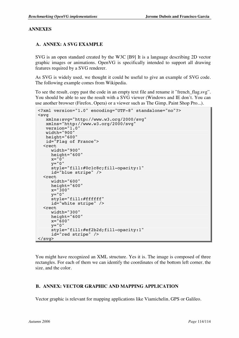
Benchmarking OpenVG implementations Jerome Dubois and Francisco Garcia
Autumn 2006 Page 114/114
ANNEXES .
A. ANNEX: A SVG EXAMPLE
SVG is an open standard created by the W3C [B9] It is a language describing 2D vector graphic images or animations. OpenVG is specifically intended to support all drawing features required by a SVG renderer.
As SVG is widely used, we thought it could be useful to give an example of SVG code. The following example comes from Wikipedia.
To see the result, copy past the code in an empty text file and rename it ”french_flag.svg”. You should be able to see the result with a SVG viewer (Windows and IE don’t. You can use another browser (Firefox, Opera) or a viewer such as The Gimp, Paint Shop Pro...). <?xml version="1.0" encoding="UTF-8" standalone="no"?> <svg xmlns:svg="http://www.w3.org/2000/svg" xmlns="http://www.w3.org/2000/svg" version="1.0" width="900" height="600" id="Flag of France"> <rect width="900" height="600" x="0" y="0" style="fill:#0c1c8c;fill-opacity:1" id="blue stripe" /> <rect width="600" height="600" x="300" y="0" style="fill:#ffffff" id="white stripe" /> <rect width="300" height="600" x="600" y="0" style="fill:#ef2b2d;fill-opacity:1" id="red stripe" /> </svg>
You might have recognized an XML structure. Yes it is. The image is composed of three rectangles. For each of them we can identify the coordinates of the bottom left corner, the size, and the color.
B. ANNEX: VECTOR GRAPHIC AND MAPPING APPLICATION
Vector graphic is relevant for mapping applications like Viamichelin, GPS or Galileo.


![Toward Patient-Speci c Myocardial · Reza Razavi, MDb, Nicholas Ayache, PhDa ... The complete 3D reconstruction of ber ori-entations from histologic sections[28], and more ... from](https://img.pdfslide.net/doc/110x75/5c4d047c93f3c34c550ae146/toward-patient-speci-c-myocardial-reza-razavi-mdb-nicholas-ayache-phda-.jpg)