REPORT OF INVESTIGATIONS/1989

Backfill Properties of Total Tailings

By C. M. K. Boldt, P. C. McWilliams, and L. A. Atkins

BUREAU OF MINES

UNITED STATES DEPARTMENT OF THE INTERIOR

Mission: As the Nation's principal conservation agency, the Departmentofthe Interior has respon­sibility for most of our nationally-owned public lands and natural and cultural resources. This includes fostering wise use of our land and water resources, protecting our fish and wildlife, pre­serving the environmental and cultural values of our national parks and historical places, and pro­viding for the enjoyment of life through outdoor recreation. The Department assesses our energy and mineral resources and works to assure that their development is in the best interests of all our people. The Department also promotes the goals of the Take Pride in America campaign by encouraging stewardship and citizen responsibil· ity for the public lands and promoting citizen par­ticipation in their care. The Department also has a major responsibility for American Indian reser­vation communities and for people who live in Island Territories under U.S. Administration.

Report of Investigations 9243

Backfill Properties of Total Tailings

By C. M. K. Boldt, P. C. McWilliams, and L. A. Atkins

UNITED STATES DEPARTMENT OF THE INTERIOR Manuel J. Lujan, Jr., Secretary

BUREAU OF MINES T S Ary, Director

CONTENTS Page

Abstract. . . . . . . . . . . . . . . . . . . . . . . . . . . . . . . . . . . . . . . . . . . . . . . . . . . . . . . . . . . . . . . . . . . . . . . . . . . 1 Introduction . . . . . . . . . . . . . . . . . . . . . . . . . . . . . . . . . . . . . . . . . . . . . . . . . . . . . . . . . . . . . . . . . . . . . . . . 2 Test procedure . . . . . . . . . . . . . . . . . . . . . . . . . . . . . . . . . . . . . . . . . . . . . . . . . . . . . . . . . . . . . . . . . . . . . . 2

Mix composition. . . . . . . . . . . . . . . . . . . . . . . . . . . . . . . . . . . . . . . . . . . . . . . . . . . . . . . . . . . . . . . . . . . 2 Mix handling ..................................................................... 4 Laboratory testing ................................................................. 4

Test analysis. . . . . . . . . . . . . . . . . . . . . . . . . . . . . . . . . . . . . . . . . . . . . . . . . . . . . . . . . . . . . . . . . . . . . . . . 4 Laboratory tests . . . . . . . . . . . . . . . . . . . . . . . . . . . . . . . . . . . . . . . . . . . . . . . . . . . . . . . . . . . . . . . . . . . 4 Statistical analysis . . . . . . . . . . . . . . . . . . . . . . . . . . . . . . . . . . . . . . . . . . . . . . . . . . . . . . . . . . . . . . . . . . 5

Discussion of results . . . . . . . . . . . . . . . . . . . . . . . . . . . . . . . . . . . . . . . . . . . . . . . . . . . . . . . . . . . . . . . . . . 9 Summary.. . . .. .. . . . . . . . . . . . . . ... . .. . . ... . . .. . . . . . .. .. . . . . ... . . . . . ... . .. . . . . . . . . . . . 11 References . . . . . . . . . . . . . . . . . . . . . . . . . . . . . . . . . . . . . . . . . . . . . . . . . . . . . . . . . . . . . . . . . . . . . . . . . 12 Appendix A.-Mix matrix and test results . . . . . . . . . . . . . . . . . . . . . . . . . . . . . . . . . . . . . . . . . . . . . . . . . . . 13 Appendix B.-Statistical definitions for goodness-of-fit ......................................... 17 Appendix C.-Linear regression results for tailings A .......................................... 18 Appendix D.-Mathematical representations and indices of determination for exponential curves relating

compressive strength to water-to-cement ratio. . . . . . . . . . . . . . . . . . . . . . . . . . . . . . . . . . . . . . . . . . . . . . 21

ILLUSTRATIONS

1. Grain-size gradation curves for tailings A, B, and C ....................................... 3 2. Grain-size gradation curves for pit-run smelter slag, ground smelter slag, and oil shale retorted waste. . . 3 3. Seven-day compressive strength versus water-to-cement ratio for tailings A ...................... 7 4. Compressive strengths versus water-to-cement ratio for total tailings data base ................... 8 5. Compressive strengths versus water-la-cement ratio for tailings A, B, and C ..................... 8 6. Compressive strengths versus water-to-cement ratio for tailings A, B, and C (not containing additives) .. 9 7. Seven-day compressive strength versus 28-, 120-, lBO-day compressive strengths, and 28-day tensile

strength for tailings A, B, and C .................................................... 10 8. Seven-day compressive strength versus 28-, 120-. 180-day compressive strengths, and 28-day tensile

strength for tailings A, B, and C (not containing additives) ................................. 11

TABLES

1. Slag chemical analysis ............................................................. 4 2. Linear correlation coefficients for tailings A variables ........................... . . . . . . . . . . . 6 3. Comparisons of goodness-of-fit for tailings A data ........................................ 7

UNIT OF MEASURE ABBREVIATIONS USED IN THIS REPORT

m inch pct percent

IbjW pound per cubic foot psi pound per square inch

m2jkg square meter per kilogram stjh short ton per hour

min minute wt pct weight percent

mm millimeter

BACKFILL PROPERTIES OF TOTAL TAILINGS

By C. M. K. Boldt,1 P. C. McWilliams,2 and L. A. Atkins3

ABSTRACT

This U.S. Bureau of Mines report presents a study of three typical tailings samples as potential cemented backfUl in underground mines. The testing series was unique in that the pulp densities of the samples were all above 75 pct solids. Test results included dry density; slump; percent settling after 28 days of curing; tensile strength after 28, 120, and 180 days of curing; and unconfined compressive strengths after 7, 28, 120, and 180 days of curing. The physical properties of the various test mixtures were further analyzed using linear and nonlinear statistical methods to produce correlations and mathematical equations. Physical properties were used to determine the influence of mix additives and as input for numerical modeling studies of backfill. The mathematical relations were used as a predictive tool in determining the suitability of various materials as backfill.

lCivil engineer. 2Mathematical statistician. 3Engineering technician. Spokane Research Center, U.S. Bureau of Mines, Spokane, WA.

2

INTRODUCTION

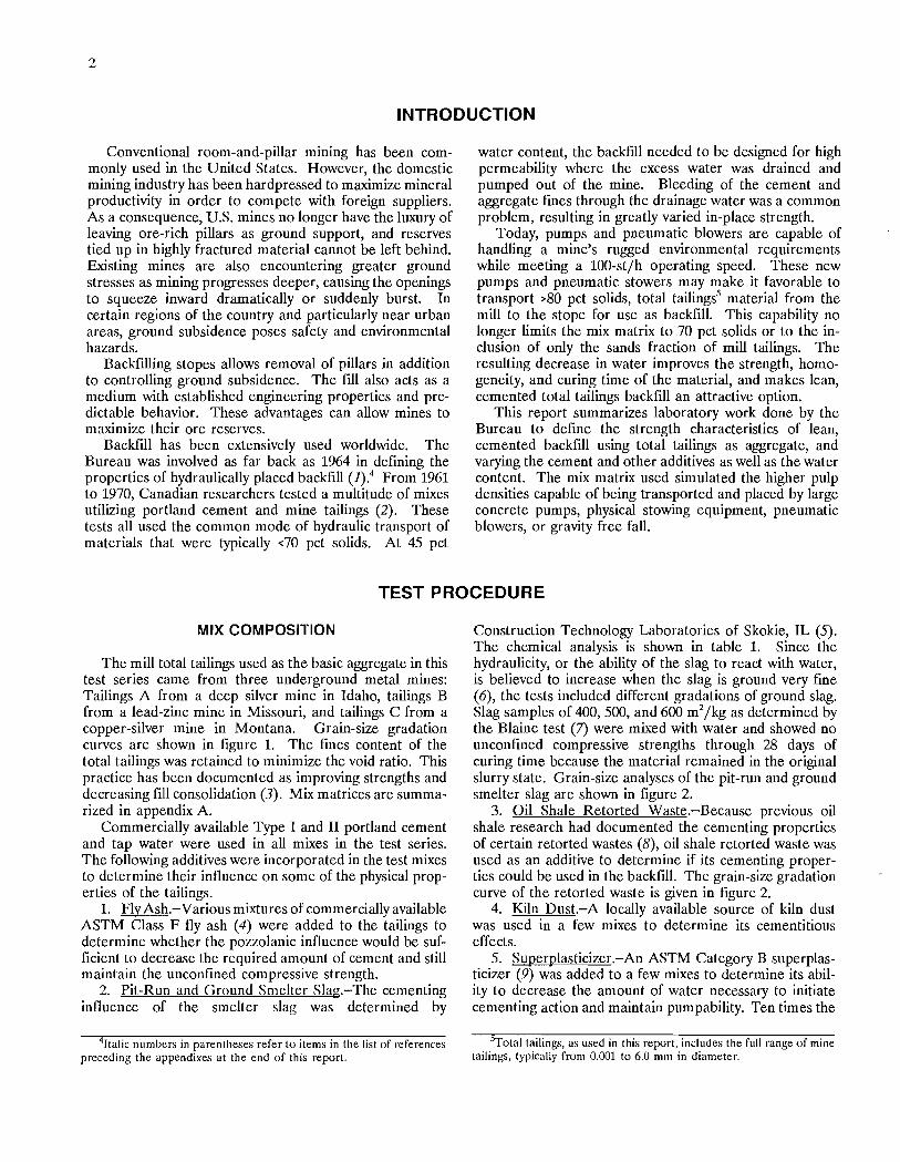
Conventional room-and-pillar mining has been com­monly used in the United States. However, the domestic mining industry has been hardpressed to maximize mineral productivity in order to compete with foreign suppliers. As a consequence, U.S. mines no longer have the luxury of leaving ore-rich pillars as ground support, and reserves tied up in highly fractured material cannot be left behind. Existing mines are also encountering greater ground stresses as mining progresses deeper, causing the openings to squeeze inward dramatically or suddenly burst. In certain regions of the country and particularly near urban areas, ground subsidence poses safety and environmental hazards.

Backfilling stopes allows removal of pillars in addition to controlling ground subsidence. The fill also acts as a medium with established engineering properties and pre­dictable behavior. These advantages can allow mines to maximize their ore reserves.

Backfill has been extensively used worldwide. The Bureau was involved as far back as 1964 in defining the properties of hydraulically placed backfill (1).4 From 1961 to 1970, Canadian researchers tested a multitude of mixes utilizing portland cement and mine tailings (2). These tests all used the common mode of hydraulic transport of materials that were typically <70 pct solids. At 45 pct

water content, the backftll needed to be designed for high permeability where the excess water was drained and pumped out of the mine. Bleeding of the cement and aggregate fines through the drainage water was a common problem, resulting in greatly varied in-place strength.

Today, pumps and pneumatic blowers are capable of handling a mine's rugged environmental requirements while meeting a 100-st/h operating speed. These new pumps and pneumatic stowers may make it favorable to transport >80 pct solids, total tailingsS material from the mill to the stope for use as backfill. This capability no longer limits the mix matrix to 70 pct solids or to the in­clusion of only the sands fraction of mill tailings. The resulting decrease in water improves the strength, homo­geneity, and curing time of the material, and makes lean, cemented total tailings backfill an attractive option.

This report summarizes laboratory work done by the Bureau to define the strength characteristics of lean, cemented backfill using total tailings as aggregate, and varying the cement and other additives as well as the water content. The mix matrix used simulated the higher pulp densities capable of being transported and placed by large concrete pumps, physical stowing equipment, pneumatic blowers, or gravity free fall.

TEST PROCEDURE

MIX COMPOSITION

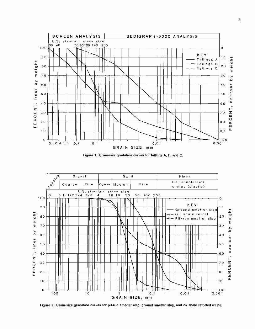
The mill total tailings used as the basic aggregate in this test series came from three underground metal mines: Tailings A from a deep silver mine in Idaho, tailings B from a lead-zinc mine in Missouri, and tailings C from a copper-silver mine in Montana. Grain-size gradation curves are shown in figure 1. The fines content of the total tailings was retained to minimize the void ratio. This practice has been documented as improving strengths and decreasing fill consolidation (3). Mix matrices are summa­rized in appendix A.

Commercially available Type I and II portland cement and tap water were used in all mixes in the test series. The following additives were incorporated in the test mixes to determine their influence on some of the physical prop­erties of the tailings.

1. Fly Ash.-Various mixtures of commercially available ASTM Class F fly ash (4) were added to the tailings to determine whether the pozzolanic influence would be suf­ficient to decrease the required amount of cement and still maintain the unconfined compressive strength.

2. Pit-Run and Ground Smelter Slag.-The cementing innuence of the smelter slag was determined by

4ltalic numbers in parentheses refer 10 items in the list of references preceding the appendixes at the end of this report.

Construction Technology Laboratories of Skokie, IL (5). The chemical analysis is shown in table 1. Since the hydraulicity, or the ability of the slag to react with water, is believed to increase when the slag is ground very fine (6), the tests included different gradations of ground slag. Slag samples of 400,500, and 600 m2/kg as determined by the Blaine test (7) were mixed with water and showed no unconfined compressive strengths through 28 days of curing time because the material remained in the original slurry state. Grain-size analyses of the pit-run and ground smelter slag are shown in figure 2.

3. Oil Shale Retorted Waste.-Because previous oil shale research had documented the cementing properties of certain retorted wastes (8), oil shale retorted waste was used as an additive to determine if its cementing proper­ties could be used in the backfill. The grain-size gradation curve of the retorted waste is given in figure 2.

4. Kiln Dust.-A locally available source of kiln dust was used in a few mixes to determine its cementitious effects.

5. Superplasticizer.-An ASTM Category B superplas­ticizer (9) was added to a few mixes to determine its abil­ity to decrease the amount of water necessary to initiate cementing action and maintain pumpability. Ten times the

5fotal tailings, as used in this report, includes the full range of mine tailings, typically from 0.001 to 6.0 mm in diameter.

.r::. OJ

Cll

3:

>-.c

Cll c:

I-Z W 0 0: W a...

.r::. OJ

OJ

3:

>-.c

OJ c:

I-Z W 0 0: W a...

100

90

80

70

60

50

40

30

20

10

0

100

90

80

70

60

50

40

30

20

10

0

SCREEN ANALYSIS SEDIGRAPH-5000 ANALYSIS u.s. standard sieve size

30 40 7080100 140 200

1'-", 1'-." r"1'--

1'- ........... KEY

"'" , -- Tailings A

r-... "- ........ -- Tailings B

'\ \ " _.- Tailings C

'-. "1\ \ "" ~ \ '" ~ "'.

o

10

20

30

40

50

60

'\ '" ~i'-~

0.50.4 0.3 0.2 0.1

'I'\. "" ........... ----...........

----.......... 0.01

GRAIN SIZE, mm

--I-

'. ~

........... " --r-----

70

80

90

............................. 1 00

0.001

Figure 1.-Grain-size gradation curves for tailings A, B, and C.

co Gravel Sand ,0

'" Coarse I Medium I '" Fine Coarse Fin e 0 CJ

U.S. standard s i e ve s i z e 6 3 1-1/23/4 3/8 4 10 16 30 50 100 200 .,-

""" r~ r'\r\

"\' \

~ \ \

r--.

\ i' \

......

1\ .........

1\ \

1\ \

i'-._.

100 10 1 0.1 GRAIN SIZE, mm

Fin e s

Silt (nonplastic)

to clay (plastic)

0

KEY 1 0

-- Ground smelter slag

-- Oil s h a Ie ret or t _.- Pit-run smelter slag

20

.... , " '\

\ .........

-........-... 1'\

0.01

",

30

40

50

60

70

80

90

100 0.001

Figure 2.-Grain-size gradation curves for pit-run smelter slag, ground smelter slag, and oil shale retorted waste.

.r::. OJ

Cll

3:

Cll (/)

co o u

I­Z W o 0: W a...

-.r::. OJ

Cll

3:

>-.c

Cll (/)

co 0 u

I-Z W 0 0: W a...

3

4

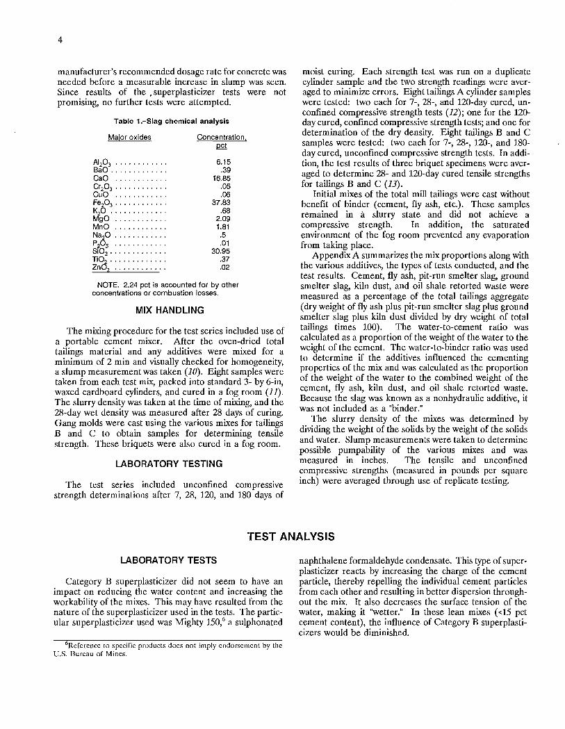
manufacturer's recommended dosage rate for concrete was needed before a measurable increase in slump was seen. Since results of the. superplasticizer tests were not promising, no further tests were attempted.

Table 1.-5Ia9 chemical analysis

Major oxides

AI20 3 ....•....... BaO ............ . CaO ........... . Cr20 3 ........... .

CuO ........... . Fe20 3 • •....•.•.•.

K20 ............ . MgO ........... . MnO ........... . Na~O ........... . P20S ........... .

Si02 ··•········· . TiO~ ............ . Zn02 ••••••••.•.•

Concentration, .I2f!

6.15 .39

16.85 .05 .06

37.83 .68

2.09 1.81

.5

.01 30.95

.37

.02

NOTE.-2.24 pct is accounted for by other concentrations or combustion losses.

MIX HANDLING

The mixing procedure for the test series included use of a portable cement mixer. After the oven-dried total tailings material and any additives were mixed for a minimum of 2 min and visually checked for homogeneity, a slump measurement was taken (10). Eight samples were taken from each test mix, packed into standard 3- by 6-in, waxed cardboard cylinders, and cured in a fog room (11). The slurry density was taken at the time of mixing, and the 28-day wet density was measured after 28 days of curing. Gang molds were cast using the various mixes for tailings Band C to obtain samples for determining tensile strength. These briquets were also cured in a fog room.

LABORATORY TESTING

The test series included unconfined compressive strength determinations after 7, 28, 120, and 180 days of

moist curing. Each strength test was run on a duplicate cylinder sample and the two strength readings were aver­aged to minimize errors. Eight tailings A cylinder samples were tested: two each for 7-, 28-, and 120-day cured, un­confined compressive strength tests (12); one for the 120-day cured, confined compressive strength tests; and one for determination of the dry density. Eight tailings Band C samples were tested: two each for 7-, 28-, 120-, and 180-day cured, unconfined compressive strength tests. In addi­tion, the test results of three briquet specimens were aver­aged to determine 28- and 120-day cured tensile strengths for tailings B and C (13).

Initial mixes of the total mill tailings were cast without benefit of binder (cement, fly ash, etc.). These samples remained in it slurry state and did not achieve a compressive strength. In addition, the saturated environment of the fog room prevented any evaporation from taking place.

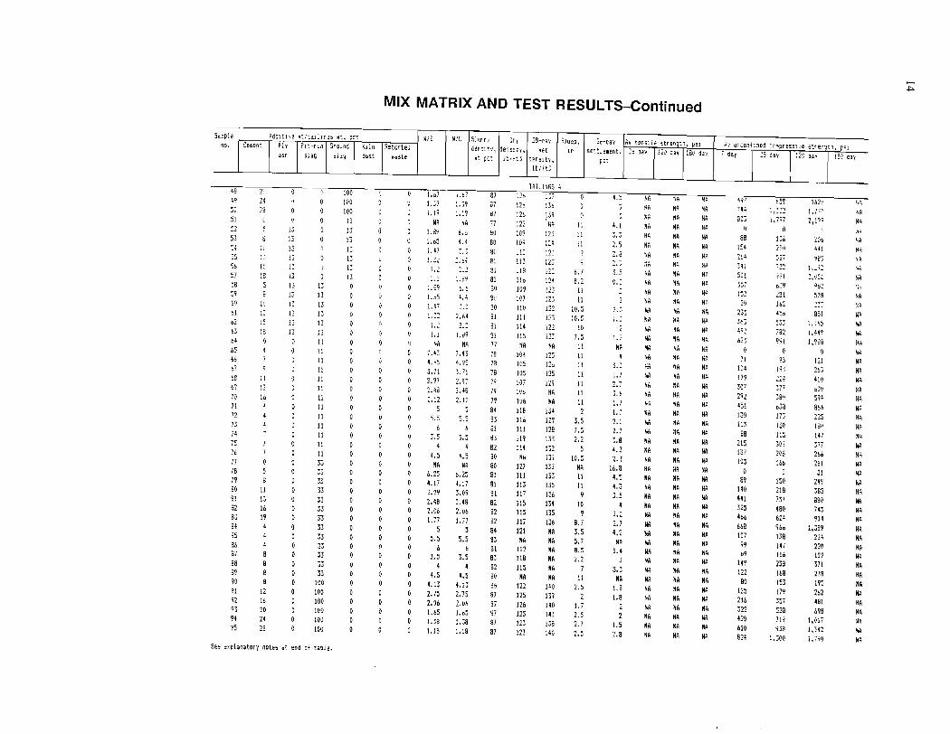
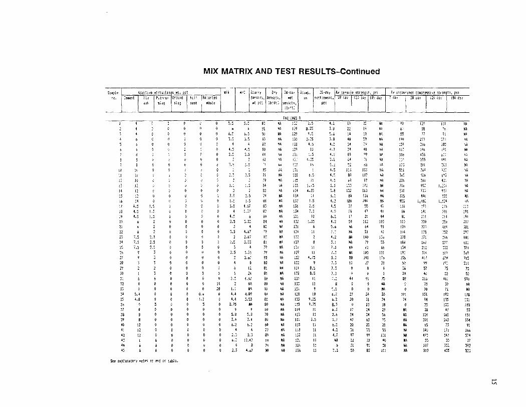
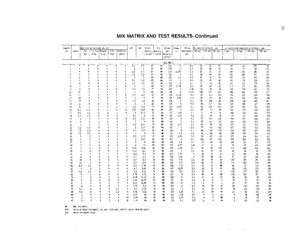
Appendix A summarizes the mix proportions along with the various additives, the types of tests conducted, and the test results. Cement, fly ash, pit-run smelter slag, ground smelter slag, kiln dust, and oil shale retorted waste were measured as a percentage of the total tailings aggregate (dry weight of fly ash plus pit-run smelter slag plus ground smelter slag plus kiln dust divided by dry weight of total tailings times 100). The water-to-cement ratio was calculated as a proportion of the weight of the water to the weight of the cement. The water-to-binder ratio was used to determine if the additives influenced the cementing properties of the mix and was calculated as the proportion of the weight of the water to the combined weight of the c~ment, fly ash, kiln dust, and oil shale retorted waste. Because the slag was known as a nonhydraulic additive, it was not included as a "binder."

The slurry density of the mixes was determined by dividing the weight of the solids by the weight of the solids and water. Slump measurements were taken to determine possible pumpability of the various mixes and was measured in inches. The tensile and unconfined compressive strengths (measured in pounds per square inch) were averaged through use of replicate testing.

TEST ANALYSIS

LABORA TORY TESTS

Category B superplasticizer did not seem to have an impact on reducing the water content and increasing the workability of the mixes. This may have resulted from the nature of the superplasticizer used in the tests. The partic­ular superplasticizer used was Mighty 150,6 a sulphonated

6Reference to specific products does not imply endorsement by the U.S. Bureau of Mines.

naphthalene formaldehyde condensate. This type of super­plasticizer reacts by increasing the charge of the cement particle, thereby repelling the individual cement particles from each other and resulting in better dispersion through­out the mix. It also decreases the surface tension of the water, making it "wetter." In these lean mixes «15 pct cement content), the influence of Category B superplasti­cizers would be diminished.

STATISTICAL ANALYSIS

At the beginning of the test series, tailings A results were statistically analyzed to determine if any meaningful relationships eXisted among the data. Ninety-five sample pairs were cast through the course of testing and included various additives such as pit-run smelter slag, ground smelter slag, and fly ash. Four candidate predicted vari­ables (variables to be predicted from mixture information) were measured: average unconfined compressive strength at 7-, 28-, and 120-day curing increments and the resulting slump value. There were five predictor variables: pit-run smelter slag, ground smelter slag, fly ash, cement, and water-to-cement ratio. The predictor variables were mixed in varying proportions to test for fill properties of the tailings.

The Minitab statistical computer program was used for most of the analytic work and the primary statistical algorithm was a multivariate linear model (14). With 14 variables involved, it was necessary to perform a preanal­ysis of the variables that would sort out some of the more spurious prior to the multivariate model fitting. Therefore, pair-wise correlation coefficients between the variables involved were examined first. These values are summa­rized in table 2 and provide a quick method to determine which variables are most highly correlated.

The matrix in table 2 is a mixture of both predictor and predicted variables, as defined previously. An absolute value of 0.8 correlation coefficient was arbitrarily chosen to delineate significance (a 1.0 correlation coefficient is a perfect fit of the line to the data points). Using this crite­rion, 10 pair-wise relationships were deemed significant; however, three of these correlations were between the de­pendent variables themselves, Le., 28-day average uncon­fined compressive strength (28DCOMP) versus 120-day average unconfined compressive strength (120DCOMP), with a correlation coefficient of 0.944.

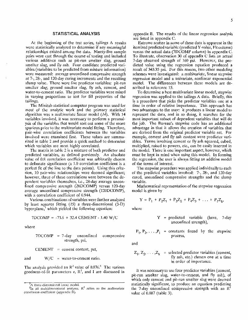
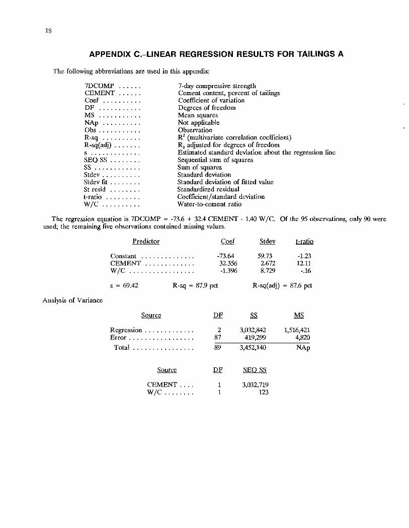
Various combinations of variables were further analyzed by least squares fitting (15) a three-dimensional (3-D) hyperplane,? which yielded the following equation:

7DCOMP :; -73.6 + 32.4 CEMENT - 1.40 W /C

where

7DCOMP

CEMENT

and W/C

7-day unconfined compressive strength, psi,

cement content, pct,

water-to-cement ratio.

The analysis provided an R 2 value of 0.876.8 The various goodness-of-fit parameters r, R2, and I are discussed in

'A three-dimensional lincar model. Srn all multidimensional analyses. R2 refers to the multivariate

correlation cocrricien( (appcndix B).

5

appendix B. The results of the linear regression analysis are listed in appendix C.

Extreme scatter in some of these data is apparent in the itemized predicted variable (predicted Y-value, Fit column) versus the actual data (7DCOMP column) in appendix C. To illustrate, observation 30 of appendix C lists an actual 7-day observed strength of 160 psi. However, the pre­dicted value using the regression equation produced a result of 343.35 psi. For this reason, two other modeling schemes were investigated: a multivariate, linear stepwise regression model and a univariate, nonlinear exponential model. The differences between these models are de­scribed in reference 15.

To determine a best multivariate linear model, stepwise regression was applied to the tailings A data. Briefly, this is a procedure that picks the predictor variables one at a time in order of relative importance. This approach has two advantages to the user: it produces a linear model to represent the data, and in so doing, it searches for the most important subset of dependent variables that will do the job. The Bureau's stepwise code has an additional advantage in that it allows the creation of variables that are derived from the original predictor variable set. For example, cement and fly ash content were predictor vari­ables. Terms involving cement or fly ash squared, cubed, multiplied, raised to powers, etc., can be easily inserted in the model. There is one important aspect, however, which must be kept in mind when using this model. In forming the regression, the user is always fitting an additive model of the terms of interest.

The stepwise procedure was applied individually to each of the predicted variables involved: 7-, 28-, and 120-day cured, unconfined compressive strengths and the slump variable.

Mathematical representation of the stepwise regression model is given by

where

Y

and

predicted variable (here, 7-day unconfined strength),

constants found by the stepwise process,

selected predictor variables (cement, fly ash, etc.) chosen one at a time in order of importance.

It was necessary to use four predictor variables (cement, pit-run smelter slag, water-to-cement, and fly ash), of which only cement and pit-run smelter slag were deemed statistically significant, to produce an equation predictin~ the 7-day unconfined compressive strength with an R value of 0.887 (table 3).

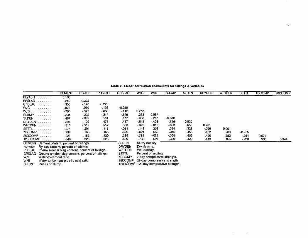
Table 2.-Unear correlation coefficients for tailings A variables

CEMENT FLYASH PRSLAG GRSLAG W/C W/B SLUMP SLDEN DRYDEN WETDEN SETTL 7DCOMP 28DCOMP FLYASH ........ 0.106 PRSLAG ........ .260 -0.222 GRSLAG ....... .353 -.170 -0.222 W/C .......... -.873 -.059 -.198 -0.259 W/B ........... -.705 -.572 -.060 -.142 0.758 SLUMP ........ -.336 .232 -.314 -.540 .283 0.057 SLDEN ......... .487 -.099 .561 .477 -.388 -.257 -0.870 DRYDEN ....... .398 -.102 .473 .457 -.548 -.408 -.726 0.820 WETDEN ....... .315 -.519 .557 .353 -.325 -.015 -.603 .653 0.701 SETTL ......... -.274 -.201 -.113 -.081 .143 .253 .334 -.328 -.096 0.001 7DCOMP ....... .939 .168 .165 .325 -.821 -.680 -.346 .456 .432 .288 -0.255 28DCOMP ...... .921 .182 .120 .389 -.781 -.671 -.358 .456 .450 .283 -.254 0.977 120DCOMP ..... .848 .326 .023 .409 -.738 -.697 -.330 .420 .443 .166 -.288 .930 0.944 CEMENT Cement content, percent of tailings. SLDEN Slurry density. FLYASH Fly ash content, percent of tailings. DRYDEN Dry density. PRSLAG Pit-run smelter slag content, percent of tailings. WETDEN Wet density. GRSLAG Ground smelter slag content, percent of tailings. SETTL Percent of settling. W/C Water-to-cement ratio 7DCOMP 7-day compressive strength. W/B Water-to-(cement-pius-flyash) ratio. 28DCOMP 28-day compressive strength. SLUMP Inches of slump. 12ODCOMP 12O-day compressive strength.

7

Table 3.-Comparlsons of goodness-of-fit for tailings A data

Model Mathematical equation Good ness­

of-fit measure

3-D hyperplane

Multivariate, linear stepwise regression

7DAVG = -73.6 + 32.4 CEMENT - 1.40 W IC ... , . , .

7DAVG = -82.58 + 33.6 CEMENT - 0.74 PRSLAG ...

if = 0.876.

R2 = 0.887.

Nonlinear, exponential. ... , , ... , , . . 7DAVG = 1 ,515.53e-0.57 WIC ................. I = 0.889.

7DAVG 7-day cured, unconfined compressive strength. R2 Multivariate correlation coefficient. CEMENT Percent cement in total aggregate contained in mix. PRSLAG Percent pit-run smelter slag contained in mix. WIC Water-to-cement ratio. I Index of determination.

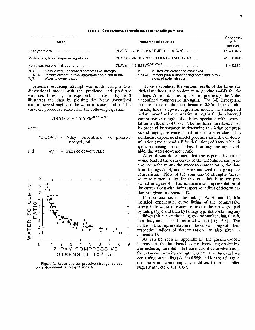
Another modeling attempt was made using a two­dimensional model with the predicted and predictor variables fitted by an exponential curve. Figure 3 illustrates the data by plotting the 7-day unconfined compressive strengths to the water-to-cement ratio. This curve-fit procedure resulted in the following equation:

7DCOMP = 1,515.53e-0.57 w/c

where

7DCOMP 7-day unconfined compressive strength, psi,

and W/C water-to-cement ratio.

I­Z ill

8f-:

~ 7

ill 6 Uo I -5

OI­l- « 4 Ie:

e: 3 ill

2 f-I­« 1 f--

?; o

• • •••• • ••• ,-.... .- .

Itf._. • I •••

· · ,··C ... • •

• •• .~"" • • .. .

• • • • •

2345678 7-DA Y COMPRESSIVE

STRENGTH, 10 2 psi

Figure 3.-Seven-day compressive strength versus water-to-cement ratio for tailings A.

9

Table 3 tabulates the various results of the three sta­tistical methods used to determine goodness-of-fit for the tailings A test data as applied to predicting the 7-day unconfined compressive strengths. The 3-D hyperplane produces a correlation coefficient of 0.876. In the multi­variate, linear stepwise regression model, the anticipated 7-day unconfined compressive strengths fit the observed compressive strengths of each test specimen with a corre­lation coefficient of 0.887. The predictor variables, listed by order of importance to determine the 7-day compres­sive strength, are cement and pit-run smelter slag. The nonlinear, exponential model produces an index of deter­mination (see appendix B for definition) of 0.889, which is quite promising since it is based on only one input vari­able, the water-to-cement ratio.

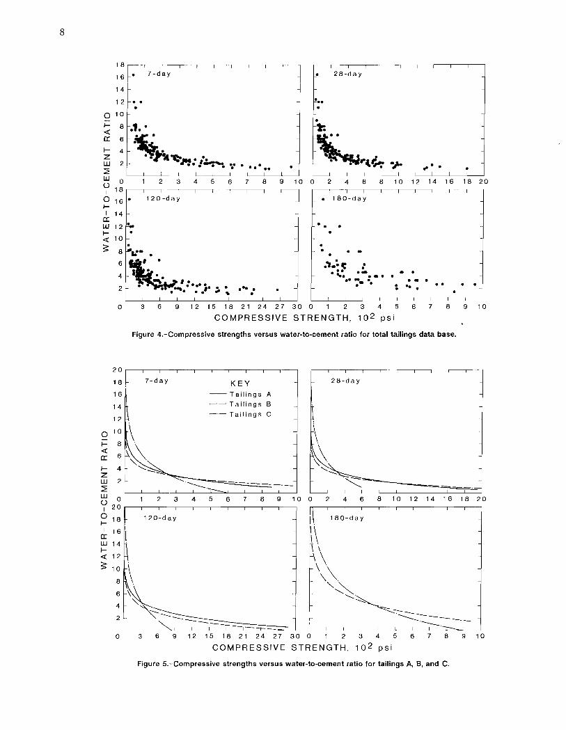
After it was determined that the exponential model would best fit the data curves of the unconfined compres­sive strengths versus the water-to-cement ratio, the data from tailings A, B; and C were analyzed as a group for comparison. Plots of the compressive strengths versus water-to-cement ratios for the total data base are pre­sented in figure 4. The mathematical representation of the curves along with their respective indices of determina­tion are given in appendix D.

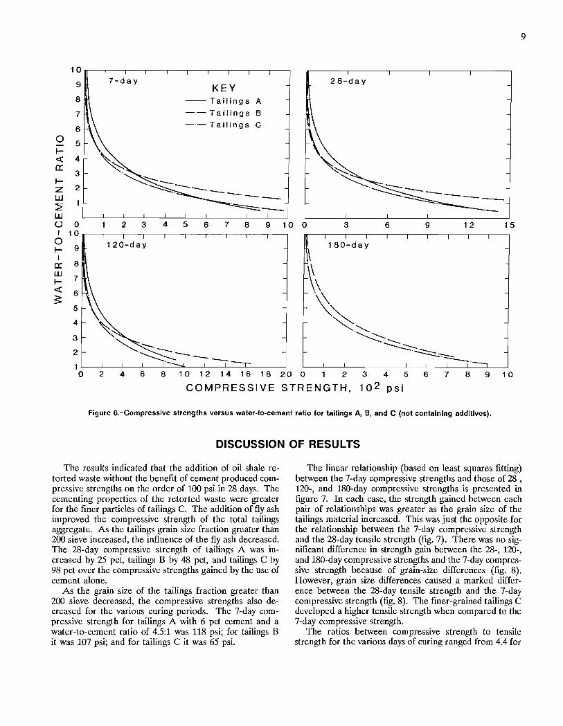
Further analysis of the tailings A, B, and C data included exponential curve fitting of the compressive strengths to water-to-cement ratios for the mixes grouped by tailings type and then by tailings type not containing any additives (pit-run smelter slag, ground smelter slag, fly ash, kiln dust, and oil shale retorted waste) (figs. 5-6). The mathematical representation of the curves along with their respective indices of determination are also given in appendix O.

As can be seen in appendix D, the goodness-of-fit increases as the data base becomes increasingly selective. For instance, the total data base index of determination, I, for 7-day compressive strength is 0.796. For the data base containing only tailings A, I is 0.889; and for the tailings A data base not containing any additives (pit-run smelter slag, fly ash, etc.), I is 0.982.

8

18

16 ~. 7 -da y ~ • 28-d a y

14

12 •• ... • •

0 10 •

f- 8 .1. • ~ «

~. ~ 0: 6

f- 4 .... . ,. ... -:.: z · ·n~.M · ,.:.-. w 2 ••• • • ... . ••• • -r .. .. ::?: •• w 0 2 3 4 5 6 7 8 9 10 0 2 4 6 8 10 12 14 16 18 20 () I 18

0 16 • 120 -day • 180-day

f-I 14

0: W 12 • • f- • « 10

~ • 8 • • • 6 • ., ... e: . • 4

• •• •• • • ... ••• • . -... . • • • • • • .. . • • • • 2 . . .... • .. .. • • 0 3 6 9 12 15 18 21 24 27 30 0 2 3 4 5 6 7 8 9 10

COMPRESSIVE STRENGTH, 10 2 psi

Figure 4.-Compressive strengths versus water-to-cement ratio for total tailings data base.

20

18 7-d a y KEY 28-day

16 -- Tailings A

14 -- Tailings B

12 -'- Tailings C

0 10 \ f- 8

\\ « 0: 6 ". f- 4 '-.: Z """ ...... W 2

---- ------::?: ---w 0 2 3 4 5 6 7 8 9 10 0 2 4 6 8 10 12 14 16 18 20 () I 20

~. 0 18 120-day 180-day f-I 16

\\ 0: w 14 f-« 1 2 \\ ~ 10 \ .

8 \\. 6 ~ "~ 4 " '-....~-:--

~----2 ---------. -- '--."'1---------0 3 6 9 12 15 18 21 24 27 30 0 2 3 4 5 6 7 8 9 10

COMPRESSIVE STRENGTH, 10 2 psi

Figure 5.-Compressive strengths versus water-to-cement ratio for tailings A, B, and C.

9

10

9 7-da y KEY

28-day

8 -- Tailings A

7 -- Tailings B

6 _.- Tailings C

0 5 I-

~ « 4 ,,~ c: 3

I- ~--- ~. :---Z 2 .~-. ------- -......:::::::: - -W - - . --~. -~ '~'-W U 0 2 3 4 5 6 7 8 9 10 0 3 6 9 12 15 I 10

0 I I I I I I I I I

I- 9 120-day

~ 180-day

I c: 8

c~\ w 7 I- -

« 6 5:

,\" 5

4 .~

~.~ 3 ~":----..... 2 f- ~~

~

1 I ~'--' 0 2 4 6 8 10 1 2 14 16 18 20 0 2 3 4 5 6 7 8 9 10

COMPRESSIVE STRENGTH, 10 2 psi

Figure 6.-Compressive strengths versus water-to-cement ratio for tailings A, 8, and C (not containing additives).

DISCUSSION OF RESULTS

The results indicated that the addition of oil shale re­torted waste without the benefit of cement produced com­pressive strengths on the order of 100 psi in 28 days. The cementing properties of the retorted waste were greater for the finer particles of tailings C. The addition of fly ash improved the compressive strength of the total tailings aggregate. As the tailings grain size fraction greater than 200 sieve increased, the influence of the fly ash decreased. The 28-day compressive strength of tailings A was in­creased by 25 pet, tailings B by 48 pet, and tailings C by 98 pet over the compressive strengths gained by the use of cement alone.

As the grain size of the tailings fraction greater than 200 sieve decreased, the compressive strengths also de­creased for the various curing periods. The 7-day com­pressive strength for tailings A with 6 pet cement and a water-to-cement ratio of 4.5:1 was 118 psi; for tailings B it was 107 psi; and for tailings C it was 65 psi.

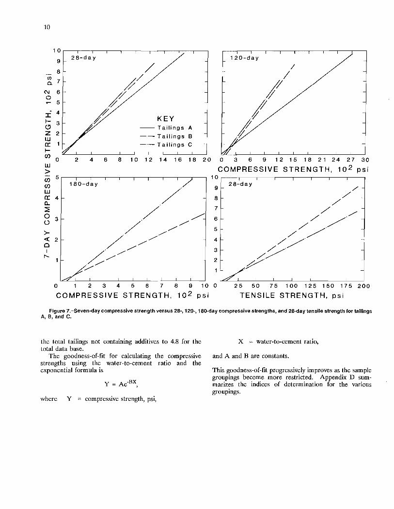
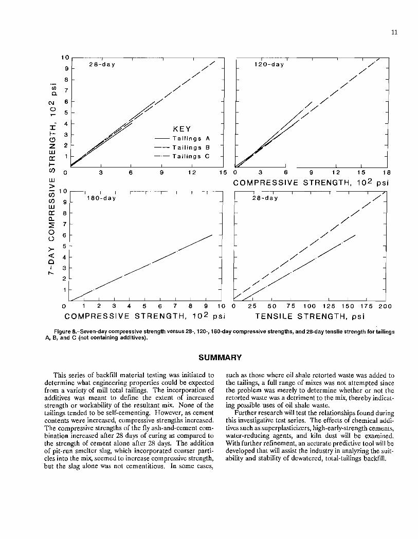
The linear relationship (based on least squares fitting) between the 7-day compressive strengths and those of 28 , 120-, and 180-day compressive strengths is presented in figure 7. In each case, the strength gained between each pair of relationships was greater as the grain size of the tailings material increased. This was just the opposite for the relationship between the 7-day compressive strength and the 28-day tensile strength (fig. 7). There was no sig­nificant difference in strength gain between the 28-, 120-, and 180-day compressive strengths and the 7-day compres­sive strength because of grain-size differences (fig. 8). However, grain size differences caused a marked differ­ence between the 28-day tensile strength and the 7-day compressive strength (fig. 8). The finer-grained tailings C developed a higher tensile strength when compared to the 7-day compressive strength.

The ratios between compressive strength to tensile strength for the various days of curing ranged from 4.4 for

10

If)

Q.

C\J 0 .....

~

::r: t-(!)

Z W a: t-

1 0

9

B

7

6

5

4

3

2

2 8-d a y

/ ~/ ~ ~

o~ KEY ---- Tailings A

-- Tailings B

_0- Tailings C

OO 0 2 4 6 B 10 12 14 16 1 B 20 0 3 6 9 12 15 1 B 21 24 27 30

W > 00 00 W a: a.. ~ 0 ()

>-« 0 I ,.....

5 1BO-day

4

3

2

COMPRESSIVE STRENGTH, 10 2 psi 10 r---.---~----.----.----.----.---'r---,

9

B

7

6

5

4

3

2

2B-day

o 1 2 3 4 5 6 7 B 9 10 0 25 50 75 100 125 150 175 200

COMPRESSIVE STRENGTH, 10 2 psi TENSILE STRENGTH, psi

Figure 7. -Seven-day compressive strength versus 28-, 120-, 180-day compressive strengths, and 28-day tensile strength for tailings A, B, and C.

the total tailings not containing additives to 4.8 for the total data base.

The goodness-of-fit for calculating the compressive strengths using the water-to-cement ratio and the exponential formula is

Y = Ae-BX ,

where Y compressive strength, psi,

x = water-to-cement ratio,

and A and B are constants.

This goodness-of-fit progressively improves as the sample groupings become more restricted. Appendix D sum­marizes the indices of determination for the various groupings.

11

10

9 2 8-d a y 120-day

8

en 7 c.. N 6 0

5 T"""

- 4 I KEY I- 3 C!) -- Tailings A Z 2 -- Tailings B W

-,- Tailings C a: I-(J) 0 3 6 9 12 15 0 3 6 9 12 15 18 W COMPRESSIVE STRENGTH, 10 2 psi > (J)

1 0 I I I I I I I I I I ,-

(J) 9 180-day

-28-da y ./

w / a: 8 / a.. / ~ 7

/ 0 6 - r- / ()

~ / ' /""

>- 5 - .// -

« 4 / - / ' -0 /.// I 3 /' ...... /// 2 /' -

~ -

t/~' 0 1 2 3 4 5 6 7 8 9 10 0 25 50 75 100 125 150 175 200

COMPRESSIVE STRENGTH, 10 2 psi TENSILE STRENGTH, psi

Figure 8.-Seven-day compressive strength versus 28-,120-, 180-day compressive strengths, and 28-day tensile strength for tailings A, B, and C (not containing additives).

SUMMARY

This series of backfill material testing was initiated to determine what engineering properties could be expected from a variety of mill total tailings. The incorporation of additives was meant to define the extent of increased strength or workability of the resultant mix. None of the tailings tended to be self-cementing. However, as cement contents were increased, compressive strengths increased. The compressive strengths of the fly ash-and-cement com­bination increased after 28 days of curing as compared to the strength of cement alone after 28 days. The addition of pit-run smelter slag, which incorporated coarser parti­cles into the mix, seemed to increase compressive strength, but the slag alone was not cementitious. In some cases,

such as those where oil shale retorted waste was added to the tailings, a full range of mixes was not attempted since the problem was merely to determine whether or not the retorted waste was a detriment to the mix, thereby indicat­ing possible uses of oil shale waste.

Further research will test the relationships found during this investigative test series. The effects of chemical addi­tives such as superplasticizers, high-early-strength cements, water-reducing agents, and kiln dust will be examined. With further refinement, an accurate predictive tool will be developed that will assist the industry in analyzing the suit­ability and stability of dewatered, total-tailings backfill.

12

REFERENCES

1. Nicholson, D. E., and W. R Wayment. Properties of Hydraulic Backfills and Preliminary Vibratory Compaction Tests. BuMines RI 6477, 1964, 31 pp.

2. Weaver, W. S., and R Luka. Laboratory Studies of Cement­Stabilized Mine Tailings. Paper in Research and Mining Applications in Cement Stabilized Backfill (pres. at 72d Annu. Gen. Meet. of Can. Inst. Min. and Metall., Toronto, Ontario, Apr. 1970). CIM, 1970, pp.988-1oo1.

3. Keren, L., and S. Kainian. Influence of Tailings Particles on Physical and Mechanical Properties of Fill. Paper in Mining With Backfill, ed. by S. Granholm (Proc. Int. Symp. on Mining With Backfill, Lulea, Sweden, June 1983). A. A. Balkema, 1983, pp. 21-29.

4. American Society for Testing and Materials. Fly Ash and Raw or Calcined Natural Pozzolan for Use as a Mineral Admixture in Portland Cement Concrete. C618-85 in 1986 Annual Book of ASTM Standards: Section 4, Volume 04.02, Concrete and Mineral Aggregate. Philadelphia, PA, 1986, pp. 385-388.

5. Weise, C. H. (Construction Technology Laboratories). Report of results, 1984; available upon request from C. M. K. Boldt, BuMines, Spokane, W A.

6. Nieminen, P., and P. Seppanen. The Use of Blast Furnace Slag and Other By-Products as Binding Agents in Consolidated Backfilling at Outokumpu Oy's Mines. Paper in Mining With Backfill, ed. by S. Granholm (Proc. of Int. Symp. of Mining With Backfill, Lulea, Sweden, June 1983). A. A. Balkema, 1983, pp. 49-58.

7. American Society for Testing and Materials. Fineness of Portland Cement by Air Permeability Apparatus. C204-84 in 1986 Annual Book of ASI'M Standards: Section 4, Volume 04.01, Cement; Lime; Gypsum. Philadelphia, PA, 1986, pp. 208-215.

8. Mareus, D., D. A. Sangrey, and S. A. Miller. Effects of Cementation Process on Spent Shale Stabilization. Min. Eng. (Littleton, CO), v. 37, 1985, pp. 1225-1232.

9. Cement Admixtures Association and the Cement and Concrete Association, Joint Working Party. Superplasticizing Admixtures in Concrete. Jan. 1976, 32 pp.

10. American Society for Testing and Materials. Slump of Portland Cement Concrete. C143-78 in 1986 Annual Book of ASTM Standards: Section 4, Volume 04.02, Concrete and Mineral Aggregates. Philadelphia, PA, 1986, pp. 109-111.

11. __ • Maldng and Curing Concrete Test Specimens in the Laboratory. CI92-81 in 1986 Annual Book of ASTM Standards: Section 4, Volume 04.02, Concrete and Minerals Aggregates. Philadelphia, PA, 1986, pp. 142-151.

12. __ . Compressive Strength of Cylindrical Concrete Specimens. C39-86 in 1986 Annual Book of ASTM Standards: Section 4, Volume 04.02, Concrete and Minerals Aggregates. Philadelphia, PA, 1986, pp. 24-29.

13. __ . Tensile Strength of Hydraulic Cement Mortars. C190-82 in 1984 Annual Book of ASTM Standards: Section 4, Volume 04.01, Cement; Lime; Gypsum. Philadelphia, PA, 1984, pp. 200-206.

14. Draper, N., and H. Smith. Applied Regression Analysis. Wiley, 1966, 407 pp.

15. McWilliams, P. C., and D. R Tesarik. Multivariate Analysis Techniques With Application in Mining. BuMines IC 8782, 1978, 40 PP.

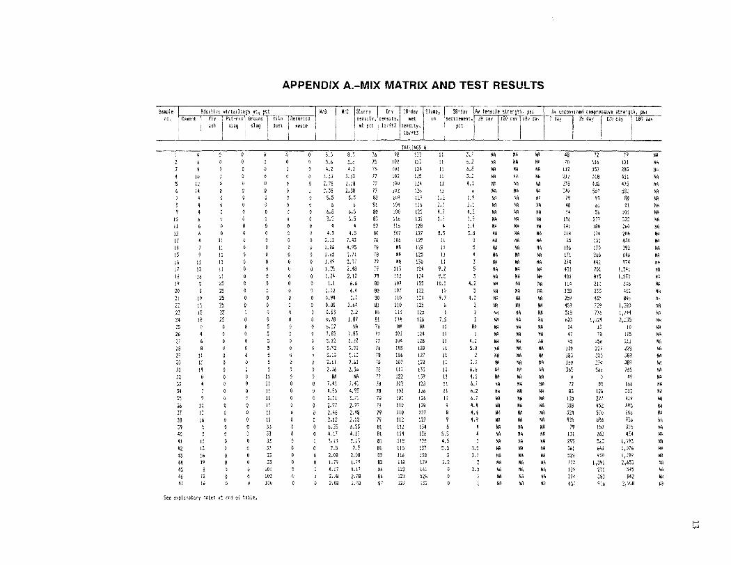
APPENDIX A.-MIX MATRIX AND TEST RESULTS

Supl. I ~dclli'te .llt,,110g5 .t, pot I wla I no. ! C!llerrt

I I

10 11 12 13 14 15 10 17 18 19 20 21 22

24 25 26

28 29 30 31 Jl

34 35 3. 31 38 39 4C 41 42 43 44 45 46 47

1" 1, 14 4 4 4

,

11 13 16

l~

15 lB o

11 13 14 o

Jl 13 16

Jl 13 16 1~

8 t2 Ie

Fly ash

, PH ron, Grouoct 1 Kiln retort., 1 I slag I slag ,dust 'a,to i

11 II 11 11 11 11 25 25 25 25 25 25 o

Ii o Ii o

11 1: 11 11 11 11 II 33 33 33 33

33 100 100 1!)0

o o o o o o o

2.7E c.38

5.5

6.5

4.5 2.12 1.86 1,;5 1. 4~

1.:5

I

1.24 1.1

1.02 C'.94 a.as 0.93 0.18 b. ~7

2.61 2.lb

7.43 4.95 3.71 2.97 2.48 2.12 •• 25 4.17

2.5 2.02 1. 79 4.17 l.lS 2.08

W,e Slurry ,I, Orr .1,28-d" SlJop, I! lB-day A, tensIle Wen\th, PSi OfflSl. tv , ,Cem!ilty, tlet in Settiflent. 2~ ddr 111Q ca, 116" da, .t pet Ilb!!tJ ,ceoslty, ' ~d

4.2 3.33 2.la 2.38

5.5

0.5 3.5

4 4.5

7.43 -1.95 l.71 2.y! 2.48 2.12 b.b 4.4

2.M

1.89 NA

7.83 5.22 3.12

NA 7.4: 4.95 ~.H

2.97 2.\3 2.12 •• 25 4.11 3.ll 2.5

2.09 1.79 4.17 2.;S 1.1;8

76 J)

77 n as 91 so 83 B1 BO 18 )9

IS 79 19 79 8(>

80 80 81 81 81 7b n 77 Ii 78 78 78 1)

78 73 ra 79 1~

19 BI 81 Bl 81 82 S2 86 So 87

i 101ft)

[ill

102 100 Ill,

l04 100 m lib lUI lOb

NA HA NA

113 i13 lQ7 107 llG 110 113 114

NA 101 104 105 lOb 107 llO 122 10:,

102 103 llD 110 112 112 HI 118 115 lib H8 122 121 l27

125 130 124 124 125 122 1:4 125 t1:; 120

UA 124 128 128 127 128 133 m 12:l 126 120 12B 127 tv 114 136 128 1.37 132 139 141 128 ll2

:

l! 11 ,I

l.2 L.] 4.7 l.'

4 9.S

11 II 11 11

9.2 9.5

10.5 10

9.7 6 6

7.5 II 11 II 11 11 11 11 11 11 11 11 9 8 9 6

5.5 4.5 5.5

3.2 o (>

o

4.~

• 1.9

4.2 2.'! 2.4 3 .•

4.2

1.3

1.2 5.9

3.3 6.b 4.l 6. J

6.2 6.7 4.4 4.4 U

I

3.5 3.7

2.5

NA NA N~

NA N~

M NA Nil NA NA NA NA HA IIA NA NA NA NA NA YA NA NA

NFl NA N,\

NA NA NA NA Nil NA NA NA NA II,

NA Nt. NA liA NA ~UI

NA NH N~

NA

NA Nri NA NA HA HA NA: NA NA N>\ NA NIl NA NA Nil hA NA NA NA NA liA NIl NA IIA NA Nil IlA liA NA NA NA NA NA IlA NA NA NA HA NA NA N~

N'; NA IiA

t\, l!ftCOflt Hied c.OlJlresslV@ str e-nqth, PSl

7 ~ai I :Ill ,ay 1 12{1 day

, IB'} aa,

I

211 218 J4(,

79

4" j4

m 141 ue

2S I~b

lH 274 431 4S! 114 159 25'1 4~9

SIB ,03 H 47 ~5

m 183 Ibll

3b5 (1

72 83

13:J 30e m 418

19 HI 295 361

772 m 27,)

406

99 &1

iTt tSO liO :31 170 1,6 Hl 701 diS 213

1,024

lG5 411 475 j83

S9 91

Z6C· 2vb m m 64b 974

l1H~

1~~~3

336 401 84(,

1,380 1,H4 2,:35

10 115 ,11 1'0 J8y 38'7 ]b~

49 166

53

55

57 58 59

61

02 63 64 65 66 67 6S 09 70 71 72

76 77 7B 79 BO 81 82 83 84 85 86 87 88 89 90 91 92 93 94 95

15 Ie

l(:

13 is 18

11 13 16

11 13 16 19 4

12 16 20 24 28

13 13 13 13 13 13 13 13 13

13

13 13 13 13

11 11 11 11 11 11 11 11 11 11 11 11 11 33

33 33 33 33 33 33 33 33 33 33 33

100 100 100 100 100 lOu

See ~~pla.rra.tory n!Jt=5 Qt ~nd of taDle.

100 100 100

13 13

13 13 13

MIX MATRIX AND TEST RESULTS-Continued

1.,7 1. ~9 1.19

HA 1.B9 1.65 1. ~7

..... " 1.2 1.1

1.89 1.,5

1.3: 1.: 1.1 ~A

7.1: 4.95 3.71 2.97 :.48 2.12

WIC

1.,7 1. ~9 1.19

NA 6., 4.4

1.89

6.6

4.4

2.64 2.:

1.89 NA

7.43 4.75

3.71 2.97 2.48

S.S .I • ..l

6

.J • .J J • .J

4.5 U NA HA

6.25 6.25 4.17 4.17 3.09 3.09 2.48 2.48 2.06 2.06 1.77 1.71

5 5.5 .J • .J

6 3.5 3.5

4 4.5 4.5

4.13 4.13 2.752.75 2.0b 1.06 1.b5 1. 65 1.';8 1.38 1.18 1.18

Slurr. Drl 2S-C!3\'

• Et

!:!!r:Sl tv, lb/ft3

den:l tv, denSl ;:1, lit ~ct 1 tift)

87 87 ,7

80 80 8(1

81 81 81

Bl' 80 81 Bl 81 1)

78 78 78 7' 79 79 B4 83 81 8.1 82 80 80 Bl 81 Bl B2 B2 B2 B4 83 81 83 81 80 B6 87 87 87 87 B7

TAILINGS A 126 137 l:':b 13tl !2b 139 122 t;A 109 109 11: 113 113 116 109 10]

Ill' III 114 I1S

NA 104 1(15

105 LO] If.\/J

lOb liB 116 111 119 114

H" 127 111 113 117 115 115 117 121

NA 112 liB 115

NA 121 125 126 125 123 123

123

I '" Lc

12,

123 122 123 122 1"

HA 125 12, 125 129

HA NA

134 p':i

128 m 132 131 13}

133 135 136 134 135 13b

NA NA ~A

NA NA NA

140 139 110 141 138 140

Sluop. 10

11 ~ 1 11

8 7

8.2 \1

11 10.5 10.5

10 7.5

11 11 11 11 11 11 11

3.5 7.5 2.2

10.~

NA 11 11

10 9

B.l 3.5 5.7 8.5 , , I..:..

11

1.7 2.5 2.7

2,-,,, 5e~ ~i e!llent •

p,t

4.5

4.1

2.5 2.a

0.:

~.::;

, .. 1.7 2.7 3.b 1.7 1.1 2.1

3.8 U 2.3

16.8 4.5 4.3 3.5

4 3.2 2.7 4.2

NA 3.4

3 3.3

NA I.B 1.8

1.5 2.B

HA NA NH

~A

HA HA Hi1 NA hA N?t NA N~

HA HA NA HA NA NA NA HA NA NA HA NA NA ItA HA NA NA HA NA ~A

HA NA HA NA MA NA MA NA NA NA NA NA MA NA NA HA NA NA HA NA NA NA KA NA

~A

NA NA NA N~

HA

I'A

NA NA IIA HA

NA NA HA IlA IIA r~A

HA NA NA HA NA 1M IIA NA NA NA NA HA NA NA NA NA NA NA NA NA NA NA NA HA NA NA

497 744 803

a8 154 i64

:4i 501 357 15:

80 233 363 4~ ~

623 o

71 1:\ 1/9

130 113

Be 215 137 103

o 89

140 441 325 4b. bbB 10) 99 69

14~

122 80

125 21b 322 420 bl0 824

659 1 ,33~ 1, 7~7

:·27

?21 6~,9

281 Ib~

450 533 782 991

o 93

19, i.1."

377 38(1

6J8 1" 130 l15 )01

20B 166

o 150 218 737 480 b24 1b6 138 147 I1b 238 lb8 153 179 357 !:2a 719 938

1,;0(1

162e'

851 1, :65 l.Hq

1,988 o

1::'1 26.3 410

377 2b6

281 31

249 365 88(' 143 914

1,J89 224 220 159 371 278 195 2b2 4B1 698

1,017 1.J4Z 1,79 r)

';I-j

liA

.IA NA ~M

~.:.

NA NA I,A NA IIA HA NA HA

NA NA HA NA IIA NA NA HA NA

II" NA HA HA HA HA NA NA HA NA NA NA HA

S,apl. no.

10 II 12

14 l~

" 17 18 19

21 n 23 24 15 26 27 28 2'1 30 31 32 33 34 35

38 39 10 4! 12 I~

44 45

It· tv 10 12

12 14

~.O 4.5 4.5

7.5 7.5 7.5

9

5. ~ 4.a

o 9 9 9

12 12 !2 6

1.5 .. , ..

" • .J

2.5 2.~

2 3 b o

o o o o

MIX MATRIX AND TEST RESULTS-Continued

0.0 1.2

5

o o o o

o 14 2B o Q

J. ,

4.~

2.~

2.~

1.0

2.: !.~

1.~

4 4.:: 2.5

3.5

2.5

1.: 4.4 4~4

2.75 ~

5.8 3.4 •• 2

4

0.2 4

2.3

WiC Slurry

de",slth ::Ia-nsth! Ifet Itt p~t lb!tt'j

0.5

4. ~

2.5 1.5

4.67 5.33

4

' •• 7 2.67 3.33

5.53 ~A

9 ~~B

3.4 0.2 , 2.3

12.47 S

4.b7

',1 30 B3 E2 BO 84

'., as 31 79 B4 82 )9

B4 Sl 82 S0 ~4

~2 1'1

85 91 79 19 82 82 81 81 80 80 80 80 BO eo 60

70 80 60 70 80 ,0 70 80

MA NA NA NA NA NA NA NA NA NA NA NA HA NA

HA NA HA NA NA NA NA

128 po

13i

131 lZS I" 113 134 m 137 !3C 134 131 132 131

131 131 132 Il0 13l 1~1

128 m 135 111 121 131

132 120 126 136

4.5 10

1.5

Iv 1

b.5 11

1.75 4,25

II 1.5 2.~

10

11 2

11 11

!1

11 3.5 II 11 11 11 11 U

3.9 S.6 j.B 4.2 4.9 4.5

4.5 3.1 3.8 6.3 4.2 4.~

4.5 0.2 4.2 5.6 7.3 • 0 .. , 3.1 7.3 7.3 5.2 7.3 7.3 1.3

5.5 6.2 b.2 B.3 6.S 2.6 3.1 b.5 1.2 4.7

NA b

7.l

52 113

89 be 13~

122 98

!~b

27 2.

o 44 o o

27 20

c3

107 Bl

171 160 !lb m

47 '35

112 64 51

140 79 .1

100 141 27

o 91

~

34 31 13 24 34 63 25

99 22 91 B5

!! 111 176 30 o

75 HA fIA 30 24 18 Z9 56 75

101

1;3 5~j

2211 ile 535 325

U6 e. Bl

110 13u 104 218 lB. 134 19;)

13. 50 3. 28 liB ()

Q

WI 74 o

!II. NA NA NA NA NA MA NIl NA

'"' 255

764

520 360

200 123

1b2 212 314 4lJ

99 57

'0 21,

3S 70

151 94 25 3.

124 201

21 107 202

92: .11 42!

1,231

2;:b 211

756

52

,81 29, BBO bl! J) I SQ9 m 2H 15 52

590 NA HA

178 131 laB 53

151 33.01

1 •• 514

37 2B2 523

MIX MATRIX AND TEST RESULTS-Continued

S-.1tI11~ 1"!Hhtl'if' ttt:tuilT1gs Itt, pet ./S WIC 28-day SltHI:P, 28-oay Ply tenHle 5tfE"ngt1'l, ;l51 Shlrry ! Dr", :10. C ... et I fh • Plt-'UT,·un; I KIln ftor"d densl tr '/ deOSl t"t. wet In settleltfnt, 28 day i 12~ a" 1180 ;.y

asn I ,l'g slag dust w .. l. wt pet, lbllt3 denSIty, pet Ib!ft3

I

to 11 12 13 14 15 16 17 IB 19 20 21 22 23 24 25 26 27 28

30 31 32 33 34 35 36 37 38 39 40 41 42 43 44 45 4b 47

a 10 10 10 12 12 12

4.5 4.5 4.5

b

1 ~:, 7.5 7.5

b 8

10 12

4.5 a

7.5

1.5 1.5 1.5

1

2.~

3

o o o

1.5 2

2.5 3 3 2 3 6

NA Hot ,Yall.ble.

o o o

o o o o

u o o o o o o o

0.6 1.2

5 o

o I)

o I)

~

I)

14 28

6 6.5

4.5 2.5

1.5

2.5 3.52

4 4.5 2.5

2 2.5

2.5

2.33 8.2 5.b 4.3 3.5 2.9 5.b 4.3 3.5

2.15 5.5B 8.21 B.21 2.92 4.4

4.42 2.77 2.04 1.14

6.5

3.5

2.5

, < < ••

•• 09 5.J3

II 3.JJ , 4.67 l.6}

.. 3.33

2.b7 B

12 4.b6 8.2 5.6 4.3 3.5 2.9

1.44 5.a9 U3 3.'n

11.15 16.42 3M5

5.9 U9 5.52

NA NA NA

NIB Ra.tio of lfat~r-to~cH~nt, fly aS~l, hIt! dust, and oil snale retorted .. aste. './e War.er-to-celent ratlo.

al 81) 83 62 80 94 82 79 95 81 79 34

il3 62 ao 64 92 79 85 61 19 79 82 82 81 80 7. 76 76 16 7. 16 76 76 76 76 16 76 76 80 80 80 80 au

NA

NA MA NA NA NA NA NA NA NA NA NA NA NA NA NA HA NA NIl NA IIA NA NA NA HA NA HA HA NA HA HA NA

!lS IH l.b25 121 123 1.5 119 123 0 125 lollS

125 1.125

124 124 2.25 121 m 0.5 125 3 .. :'5 13·) m 124 1.75 l27

m 2.25 m 126 0.5 125 0.75 125 1.15 120 1 III 1.25 1!8 1.25 121 7.5 120 7.5 118 7.5 119 3.25 120 9.5 121 10 122 11 121 11 123 11 123 11

124 2.25 125 3.75 122 2.75 122 2.5

4.2 l.b 3.1 4.2 4.2 2.1 4.2

2.06 1.04 3.1 6.3 2.1 4.2 3.1 3.1 3.1 4.2 4.2

3.1 2~ 1 3.1 3.5 :.8 3.1 3.1 3.B 3.1 3.1

!

< < •• J

20 23 50 41 33 11 45 50

128 82 55

142 7B 9b 44 37 32 n S5 40 19 BIl 45 89

128 23 o

48 16 28 35 50 56 15 25 52 NA 13 o o

2S 20 21

II

72 45 69 69 56 m III 67

16E 117 114

17 46 44

!l4 102 eo

us 121 94 IO~

157 4. o

83 19 1S ~9

5\ 71 11 51 51 ~~

6 o o

89 37 34

28 29 82 71 45 8, 69 bO

16\ 144 82

168 130 l2! 82 GO 58

135 P'

1D2 140

85 lvl 185 50 o

105 I?

51 60 82 ~A 47 74 NA 10

62 45 43 lB NA NA

NV : .. mconnr:ed :otpressnl! strenqH, pSI 7 oay

100 192 127 65

17: 174 14\

Jab 195 140 558

\

ii' 335 146 145 b9

286 2Db 159 J27 276 175 271 m 109 ))

173 39 63 91

14S 171 46 83

114 132

4b 32 27 81 78 a7 U o o

23 ~iY 112Q day

I !

21)

tt8 50~

~67

!\5 796 m 430 194 202 11:' ~n 3{)(1

223 435 391 250 376 596 131

94 lBli 55

100 129 195 243

a1 120 In 207

54 39 37

129 U5 82 78 39

103

lBa 186 19! 183 !38

221 645 Sus 242 eo'? 519 ~09

293 267 lBO 556 410 303 712 ~H

350 50b B21} 1.77 109 4:'4 50 90

136 240 21]1]

113 m 250 317

B3 47 52

241 135 l!J 11>5

43 130

IBI) oay

59 101 153 258 347 106 180 27! 33B IDS 63 56

306 151 124 199

NA NA

17

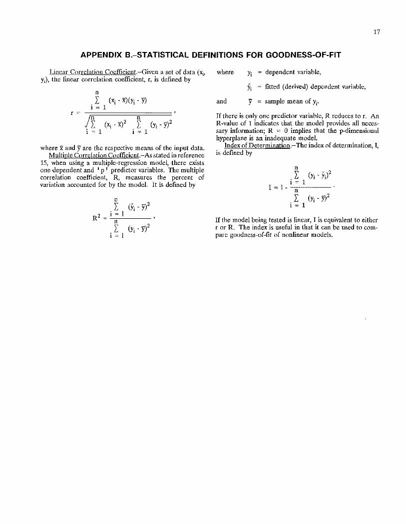
APPENDIX B.-STATISTICAL DEFINITIONS FOR GOODNESS-OF-FIT

Linear Correlation Coefficient.-Given a set of data (X;, where Yj == dependent variable, yJ, the linear correlation coefficient, r, is defmed by

n

. I (xt - X)(Yj - y) I = 1

r ==

where x and yare the respective means of the input data. MUltiple Correlation Coefficient.-As stated in reference

15, when using a multiple-regression model, there exists one dependent and 'p' predictor variables. The multiple correlation coefficient, R, measures the percent of variation accounted for by the model. It is defined by

n I

R2 '" 1 --:::"n----

I I

Yi == fitted (derived) dependent variable,

and y == sample mean of Yj.

If there is only one predictor variable, R reduces to r. An R-value of 1 indicates that the model provides all neces­sary information; R == 0 implies that the p-dimensional hyperplane is an inadequate model.

Index of Determination.-The index of determination, I, is defmed by

n I (Yi - yi

i == 1 r == I - --=-n----

I (Yi - yi 1 = 1

If the model being tested is linear, I is equivalent to either r or R. The index is useful in that it can be used to com­pare goodness-of-fit of nonlinear models.

18

APPENDIX C.-LINEAR REGRESSION RESULTS FOR TAILINGS A

The following abbreviations are used in this appendix:

IDCOMP ..... . CEMENT ..... . Coef ......... . DF .......... . MS .......... . NAp ......... . Obs .......... . R-sq ......... . R-sq(adj) ...... . s ............ . SEQ SS ....... . SS ........... . Stdev ......... . Stdev fit ....... . St resid ....... . t-ratio ........ . W/C ......... .

7-day compressive strength Cement content, percent of tailings Coefficient of variation Degrees of freedom Mean squares Not applicable Observation R2 (multivariate correlation coefficient) Rz adjusted for degrees of freedom Estimated standard deviation about the regression line Sequential sum of squares Sum of squares Standard deviation Standard deviation of fitted value Standardized residual Coefficient/standard deviation Water-to-cement ratio

The regression equation is 7DCOMP = -73.6 + 32.4 CEMENT - 1.40 W /e. Of the 95 observations, only 90 were used; the remaining five observations contained missing values.

Analysis of Variance

Predictor

Constant ............. . CEMENT ............ . W/C ................ .

-73.64 32.356 -1.396

s = 69.42 R-sq = 87.9 pct

DF

Regression ............ . 2 Error ................ . 87

Total ............... . 89

DF

CEMENT ... . 1 W/C ....... . 1

59.73 2.672 8.729

-1.23 12.11

-.16

R-sq(adj) = 87.6 pct

SS MS

3,032,842 1,516,421 419,299 4,820

3,452,140 NAp

SEQSS

3,032,719 123

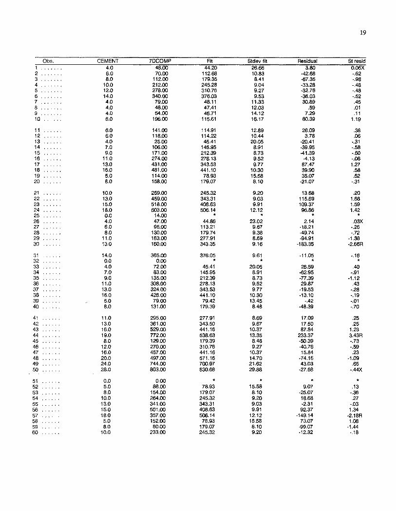
19

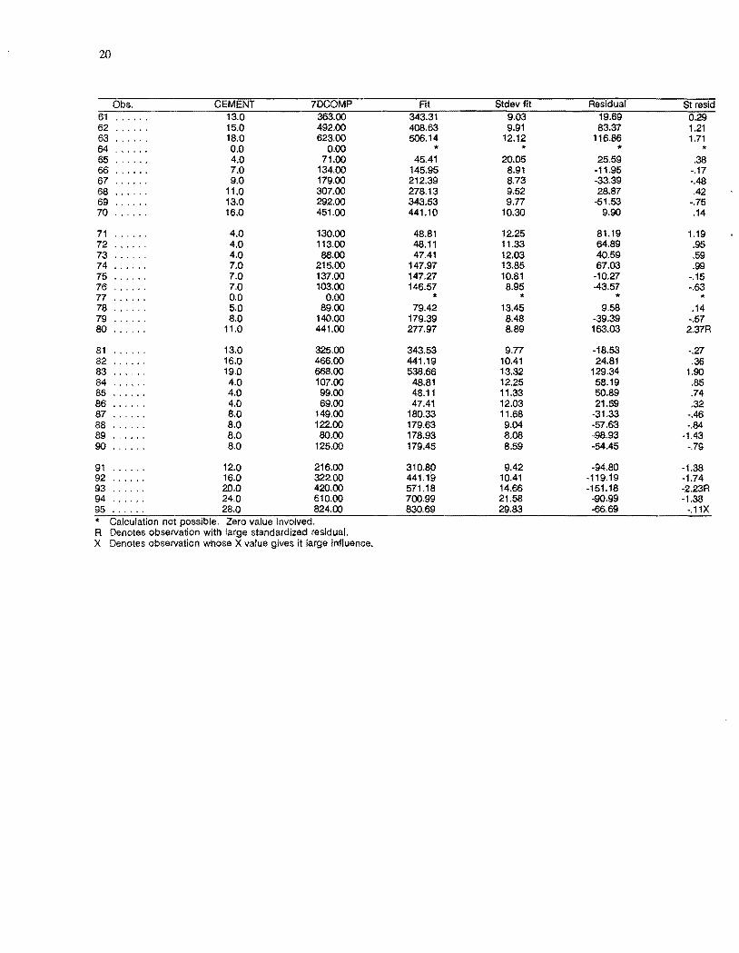
Obs. CEMENT 7DCOMP Fit 8tdev fit Residual 8t resid 1 4.0 48.00 44.20 26.66 3.80 O.06X 2 6.0 70.00 112.68 10.83 -42.68 -.62 3 8.0 112.00 179.35 8.41 -67.35 -.98 4 10.0 212.00 245.28 9.04 -33.28 -.48 5 12.0 278.00 310.76 9.27 -32.76 -.48 6 .. ,. '" 14.0 340.00 376.03 9.53 -36.03 -.52 7 4.0 79.00 48.11 11.33 30.89 .45 8 4.0 48.00 47.41 12.03 .59 .01 9 4.0 54.00 46.71 14.12 7.29 .11 10 6.0 196.00 115.61 16.17 80.39 1.19

11 6.0 141.00 114.91 12.89 26.09 .38 12 6.0 118.00 114.22 10.44 3.78 .06 13 4.0 25.00 45.41 20.05 -20.41 -.31 14 7.0 106.00 145.95 8.91 -39.95 -.58 15 9.0 171.00 212.39 8.73 -41.39 -.60 16 11.0 274.00 278.13 9.52 -4.13 -.06 17 13.0 431.00 343.53 9.77 87.47 1.27 18 16.0 481.00 441.10 10.30 39.90 .58 19 5.0 114.00 78.93 15.58 35.07 .52 20 8.0 158.00 179.07 8.10 -21.07 -.31

21 10.0 259.00 245.32 9.20 13.68 .20 22 13.0 459.00 343.31 9.03 115.69 1.68 23 15.0 518.00 408.63 9.91 109.37 1.59 24 18.0 603.00 506.14 12.12 96.86 1.42 25 0.0 14.00 " " " .. 26 4.0 47.00 44.86 23.02 2.14 .03X 27 6.0 95.00 113.21 9.67 -18.21 -.26 28 8.0 130.00 179,74 9.38 -49.74 -.72 29 11.0 183.00 277.91 8.69 -94.91 -1.38 30 13.0 160.00 343.35 9.16 -183.35 -2.66R

31 14.0 365.00 376,05 9.61 -11.05 -.16 32 0.0 0.00 * " " " 33 4.0 72.00 45.41 20.05 26.59 .40 34 7.0 83.00 145.95 8.91 -62.95 -.91 35 9.0 135.00 212.39 8.73 -77.39 -1.12 36 11.0 308.00 278.13 9.52 29.87 .43 37 13.0 324.00 343.53 9.77 -19.53 -.28 38 16.0 428.00 441.10 10.30 -13.10 ·.19 39 5.0 79.00 79.42 13.45 -.42 ·.01 40 8.0 131.00 179.39 8.48 -48.39 -.70

41 11.0 295.00 277.91 8.69 17.09 .25 42 13.0 361.00 343.50 9.67 17.50 .25 43 16.0 529.00 441.16 10.37 87.84 1.28 44 19.0 772.00 538.63 13.35 233.37 3.43R 45 8.0 129.00 179.39 8.48 -50.39 -.73 46 12.0 270.00 310.76 9.27 -40.76 -.59 47 16.0 457.00 441.16 10.37 15.84 .23 48 20.0 497.00 571.16 14.70 -74.16 -1.09 49 24.0 744.00 700.97 21.62 43.03 .65 50 28.0 803.00 830.68 29.88 -27.68 ·.44X

51 0.0 0.00 " " " " 52 5.0 88.00 78.93 15.58 9.07 .13 53 8.0 154.00 179.07 8.10 -25.07 -.36 54 10.0 264.00 245.32 9.20 18.68 .27 55 13.0 341.00 343.31 9.03 -2.31 -.03 56 15.0 501.00 408.63 9.91 92.37 1.34 57 18.0 357.00 506.14 12.12 -149.14 -2.18R 58 5.0 152.00 78.93 15.58 73.07 1.08 59 8.0 80.00 179.07 8.10 -99.07 -1.44 60 10.0 233.00 245.32 9.20 -12.32 -.18

20

Obs. CEMENT 7DCOMP Fit Stdev fit Residual St resid 61 13.0 363.00 343.31 9.03 19.69 0.29 62 15.0 492.00 408.63 9.91 83.37 1.21 63 18.0 623.00 506.14 12.12 116.86 1.71 64 0.0 0.00 " " .. * 65 4.0 71.00 45.41 20.05 25.59 .38 66 7.0 134.00 145.95 8.91 -11.95 -.17 67 9.0 179.00 212.39 8.73 -33.39 -.48 68 11.0 307.00 278.13 9.52 28.87 .42 69 13.0 292.00 343.53 9.77 -51.53 -.75 70 16.0 451.00 441.10 10.30 9.90 .14

71 4.0 130.00 48.81 12.25 81.19 1.19 72 4.0 113.00 48.11 11.33 64.89 .95 73 4.0 88.00 47.41 12.03 40.59 .59 74 7.0 215.00 147.97 13.85 67.03 .99 75 7.0 137.00 147.27 10.81 -10.27 -.15 76 7.0 103.00 146.57 8.95 -43.57 -.63 77 0.0 0.00 .. .. * * 78 5.0 89.00 79.42 13.45 9.58 .14 79 8.0 140.00 179.39 8.48 -39.39 -.57 eo 11.0 441.00 277.97 8.89 163.03 2.37R

81 13.0 325.00 343.53 9.77 -18.53 -.27 82 16.0 466.00 441.19 10.41 24.81 .36 83 19.0 668.00 538.66 13.32 129.34 1.90 84 4.0 107.00 48.81 12.25 58.19 .85 85 4.0 99.00 48.11 11.33 50.89 .74 86 4.0 69.00 47.41 12.03 21.59 .32 87 8.0 149.00 180.33 11.68 -31.33 -.46 88 8.0 122.00 179.63 9.04 -57.63 -.84 89 8.0 eo.OO 178.93 8.08 -98.93 -1.43 90 8.0 125.00 179.45 8.59 -54.45 -.79

91 12.0 216.00 310.80 9.42 -94.80 -1.38 92 16.0 322.00 441.19 10.41 -119.19 -1.74 93 20.0 420.00 571.18 14.66 -151.18 -2.23R 94 24.0 610.00 700.99 21.58 -90.99 -1.38 95 28.0 824.00 830.69 29.83 -66.69 -.11X

* Calculation not possible. Zero value involved. R Denotes observation with large standardized residual. X Denotes observation whose X value gives it large influence.

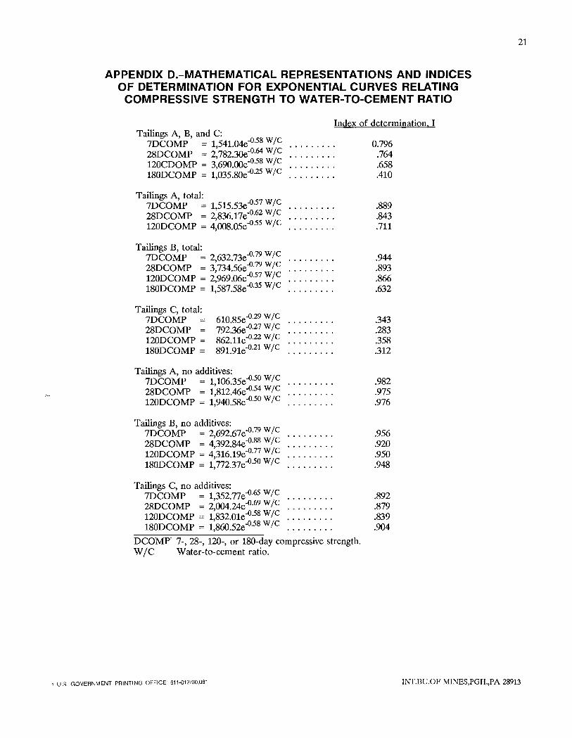
APPENDIX D.-MATHEMATICAL REPRESENTATIONS AND INDICES OF DETERMINATION FOR EXPONENTIAL CURVES RELATING

COMPRESSIVE STRENGTH TO WATER-TO-CEMENT RATIO

Tailings A, B, and C: IDCOMP = 1,541.04e-O.58 w/e 28DCOMP = 2,782.30e-O.64 w/e 120CDOMP = 3,690.00e-O·58 W Ie 180DCOMP = 1,035.80e-O.25 W Ie

Tailings A, total: IDCOMP = 1,515.53e-O.57 w/e 28DCOMP = 2,836.17e-O.62 w/e 120DCOMP = 4,OO8.05e-O·55 W Ie

Tailings B, total: IDCOMP = 2,632.73e-O.79 W Ie 28DCOMP = 3,734.56e-O.79 w/e 120DCOMP = 2,969.06e-O.57 W Ie 180DCOMP = 1,587.58e-O.35 W Ie

Tailings C, total: IDCOMP 28DCOMP = 120DCOMP = 180DCOMP =

61O.85e-O.29 w/e 792.36e-O.27 W Ie 862.11e-O.22 W Ie 891.91e-O.21 W Ie

Tailings A, no additives: 7DCOMP = 1,106.35e-O.50 w/e 28DCOMP = 1,812.46e-O.54 W Ie 120DCOMP = 1,940.58e-O.50 w/e

Tailings B, no additives: 7DCOMP = 2,692.67e-O.79 W Ie 28DCOMP = 4,392.84e-O.88 w/e 120DCOMP = 4,316.1ge-O.77 W Ie 180DCOMP = 1,772.37e-O.50 W Ie

Index of determination, I

0.796 .764 .658 .410

.889

.843

.711

.944

.893

.866

.632

.343

.283

.358

.312

.982

.975

.976

.956

.920

.950

.948

Tailings C, no additives: 7DCOMP = 1,352.77e-O.65 w/e ......... .892 28DCOMP = 2,OO4.24e-O.69 W Ie ......... .879 120DCOMP = 1,832.01e-O.58 w/e ......... .839 180DCOMP = 1,860.52e-O.58 W Ie ......... .904

DCOMP 7-,28-, 120-, or 180-day compressive strength. W IC Water-to-cement ratio.

21

~ u.s. GOVERNMENT PRINTING OFFICE 611-012/00.081 Il\'T.I3U.OF MINES,PGH.,PA 28913