Embed Size (px)
Citation preview
Basic Business Statistics, 10e © 2006 Prentice-Hall, Inc.. Chap 11-1
Chapter 11
Analysis of Variance
Basic Business Statistics10th Edition
Basic Business Statistics, 10e © 2006 Prentice-Hall, Inc. Chap 11-2
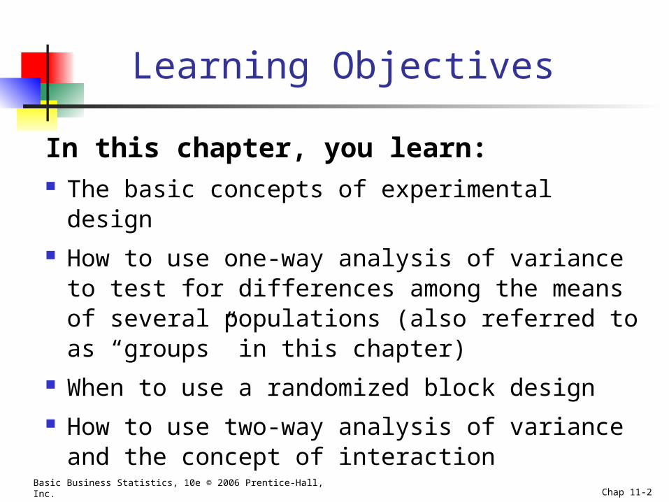
Learning Objectives
In this chapter, you learn: The basic concepts of experimental design How to use one-way analysis of variance to test
for differences among the means of several populations (also referred to as “groups” in this chapter)
When to use a randomized block design How to use two-way analysis of variance and the
concept of interaction
Basic Business Statistics, 10e © 2006 Prentice-Hall, Inc. Chap 11-3
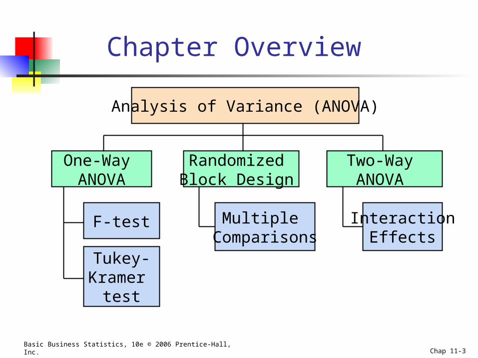
Chapter Overview
Analysis of Variance (ANOVA)
F-test
Tukey-Kramer
test
One-Way ANOVA
Two-Way ANOVA
InteractionEffects
Randomized Block Design
Multiple Comparisons
Basic Business Statistics, 10e © 2006 Prentice-Hall, Inc. Chap 11-4
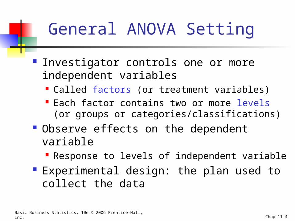
General ANOVA Setting
Investigator controls one or more independent variables Called factors (or treatment variables) Each factor contains two or more levels (or groups or
categories/classifications) Observe effects on the dependent variable
Response to levels of independent variable Experimental design: the plan used to collect
the data
Basic Business Statistics, 10e © 2006 Prentice-Hall, Inc. Chap 11-5
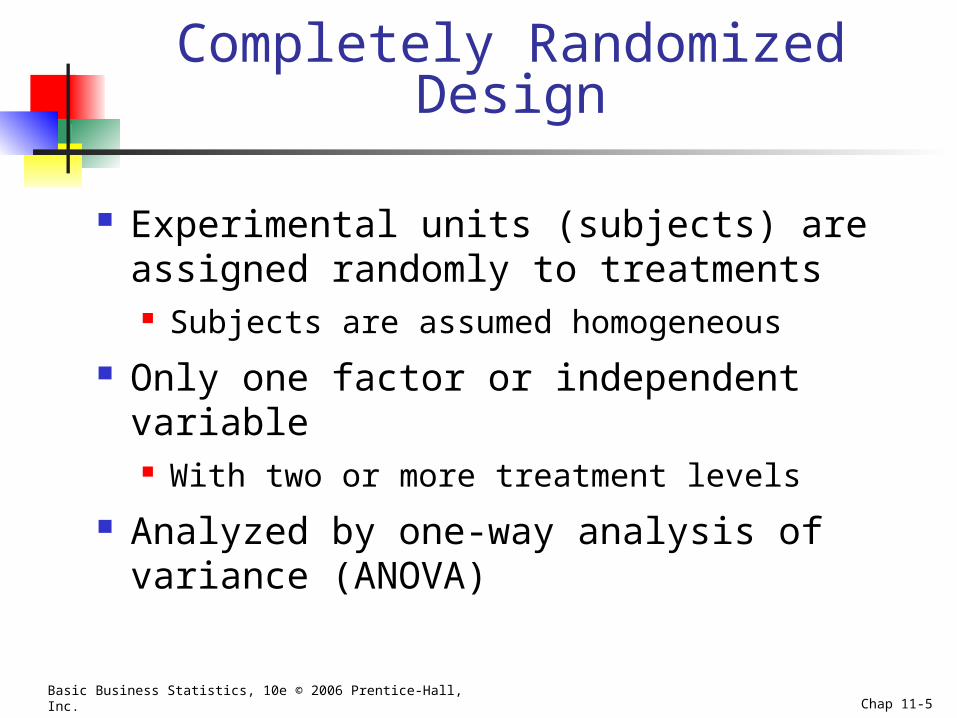
Completely Randomized Design
Experimental units (subjects) are assigned randomly to treatments Subjects are assumed homogeneous
Only one factor or independent variable With two or more treatment levels
Analyzed by one-way analysis of variance (ANOVA)
Basic Business Statistics, 10e © 2006 Prentice-Hall, Inc. Chap 11-6
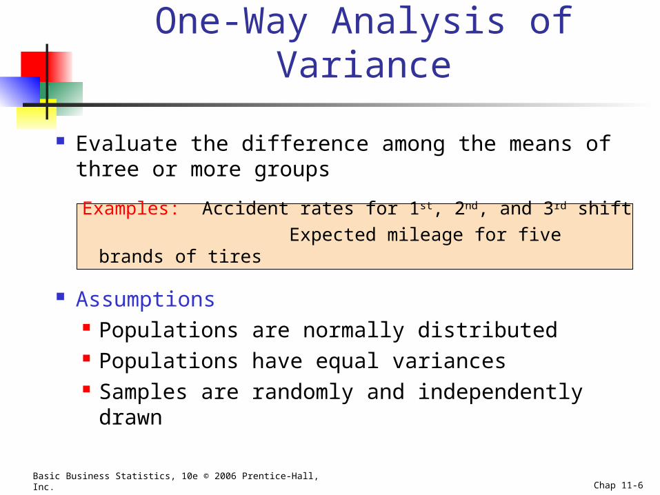
One-Way Analysis of Variance
Evaluate the difference among the means of three or more groups
Examples: Accident rates for 1st, 2nd, and 3rd shift
Expected mileage for five brands of tires
Assumptions Populations are normally distributed Populations have equal variances Samples are randomly and independently drawn
Basic Business Statistics, 10e © 2006 Prentice-Hall, Inc. Chap 11-7
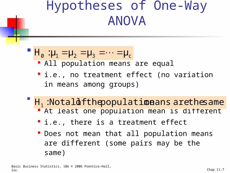
Hypotheses of One-Way ANOVA
All population means are equal i.e., no treatment effect (no variation in means among
groups)
At least one population mean is different i.e., there is a treatment effect Does not mean that all population means are different
(some pairs may be the same)
c3210 μμμμ:H
same the are means population the of all Not:H1
Basic Business Statistics, 10e © 2006 Prentice-Hall, Inc. Chap 11-8
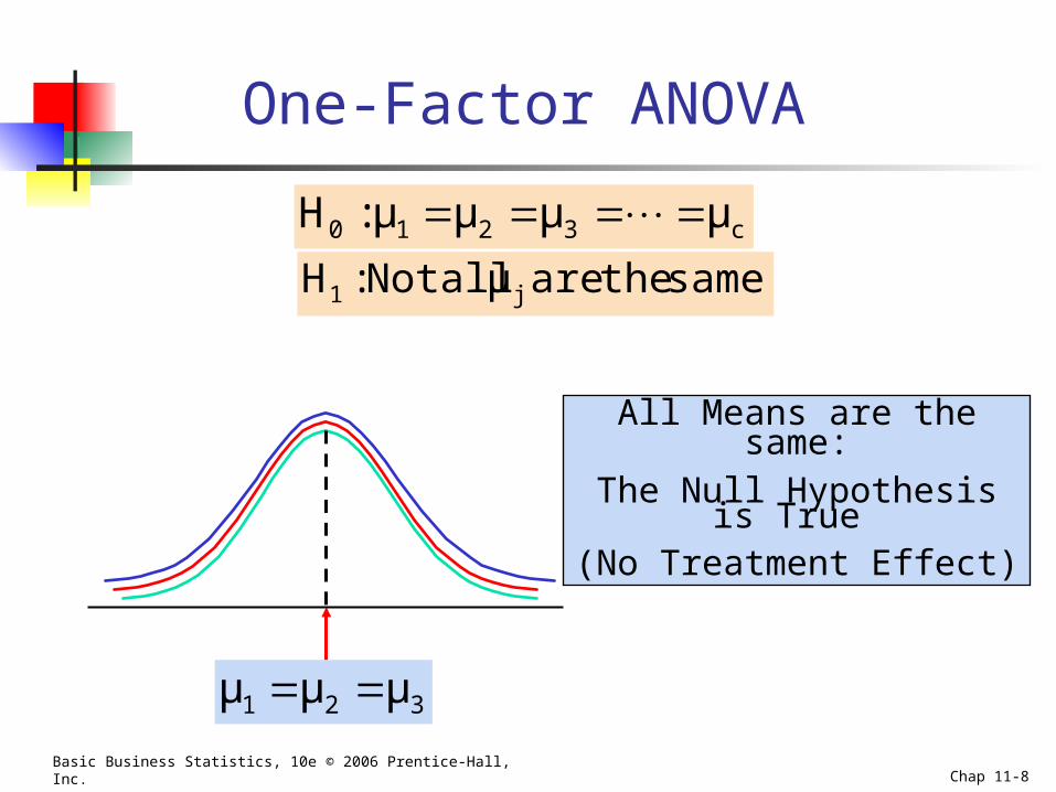
One-Factor ANOVA
All Means are the same:The Null Hypothesis is True
(No Treatment Effect)
c3210 μμμμ:H same the are μ all Not:H j1
321 μμμ
Basic Business Statistics, 10e © 2006 Prentice-Hall, Inc. Chap 11-9
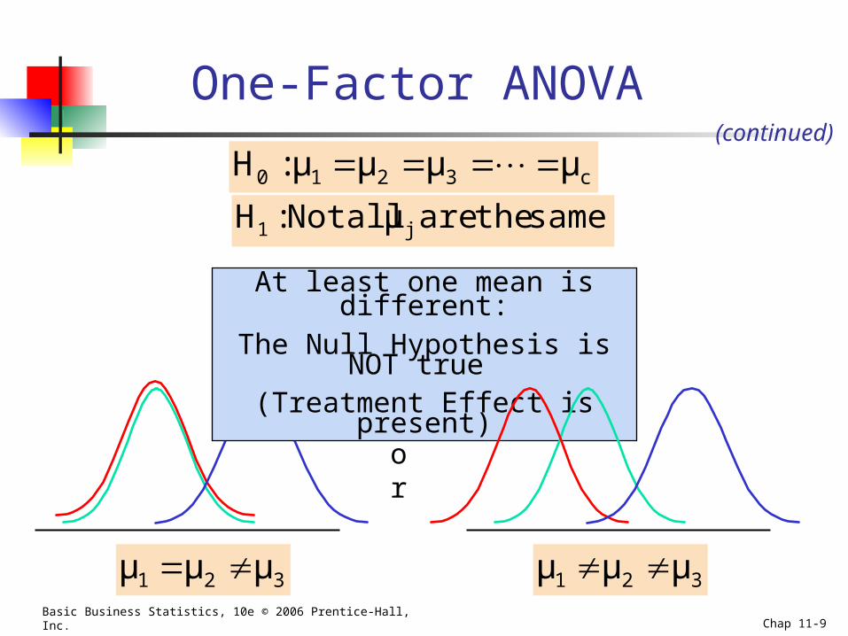
One-Factor ANOVA
At least one mean is different:The Null Hypothesis is NOT true
(Treatment Effect is present)
c3210 μμμμ:H same the are μ all Not:H j1
321 μμμ 321 μμμ
or
(continued)
Basic Business Statistics, 10e © 2006 Prentice-Hall, Inc. Chap 11-10
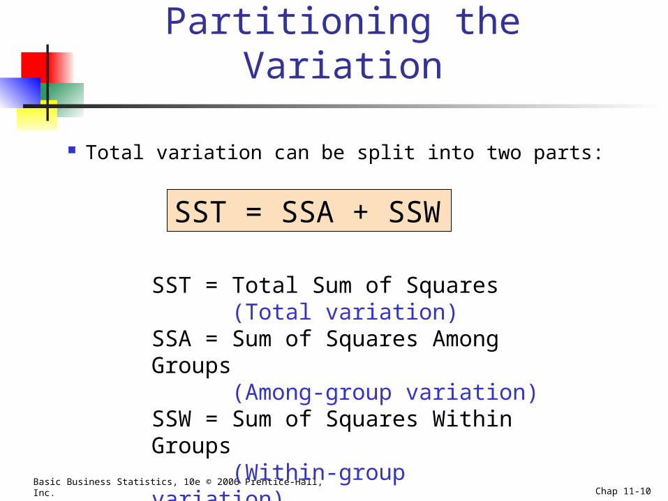
Partitioning the Variation
Total variation can be split into two parts:
SST = Total Sum of Squares (Total variation)
SSA = Sum of Squares Among Groups (Among-group variation)
SSW = Sum of Squares Within Groups (Within-group variation)
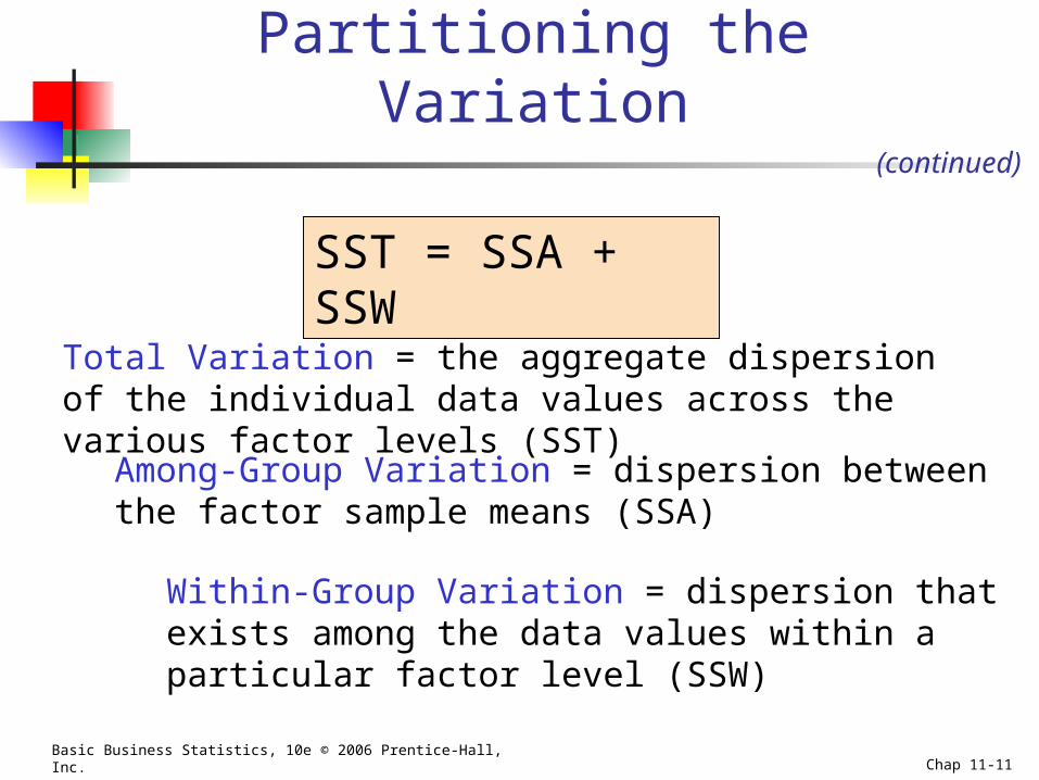
SST = SSA + SSW
Basic Business Statistics, 10e © 2006 Prentice-Hall, Inc. Chap 11-11
Partitioning the Variation
Total Variation = the aggregate dispersion of the individual data values across the various factor levels (SST)
Within-Group Variation = dispersion that exists among the data values within a particular factor level (SSW)
Among-Group Variation = dispersion between the factor sample means (SSA)
SST = SSA + SSW
(continued)

Basic Business Statistics, 10e © 2006 Prentice-Hall, Inc. Chap 11-12
Partition of Total Variation
Variation Due to Factor (SSA)
Variation Due to Random Sampling (SSW)
Total Variation (SST)
Commonly referred to as: Sum of Squares Within Sum of Squares Error Sum of Squares Unexplained Within-Group Variation
Commonly referred to as: Sum of Squares Between Sum of Squares Among Sum of Squares Explained Among Groups Variation
= +
d.f. = n – 1
d.f. = c – 1 d.f. = n – c
Basic Business Statistics, 10e © 2006 Prentice-Hall, Inc. Chap 11-13
Total Sum of Squares
c
1j
n
1i
2ij
j
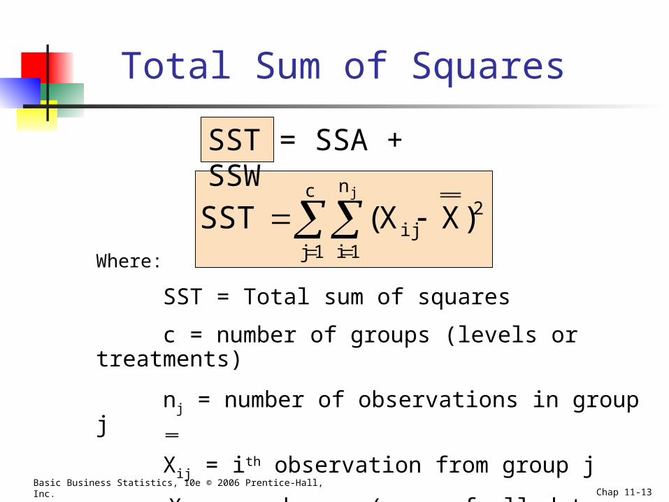
)XX(SSTWhere:
SST = Total sum of squares
c = number of groups (levels or treatments)
nj = number of observations in group j
Xij = ith observation from group j
X = grand mean (mean of all data values)
SST = SSA + SSW
Basic Business Statistics, 10e © 2006 Prentice-Hall, Inc. Chap 11-14
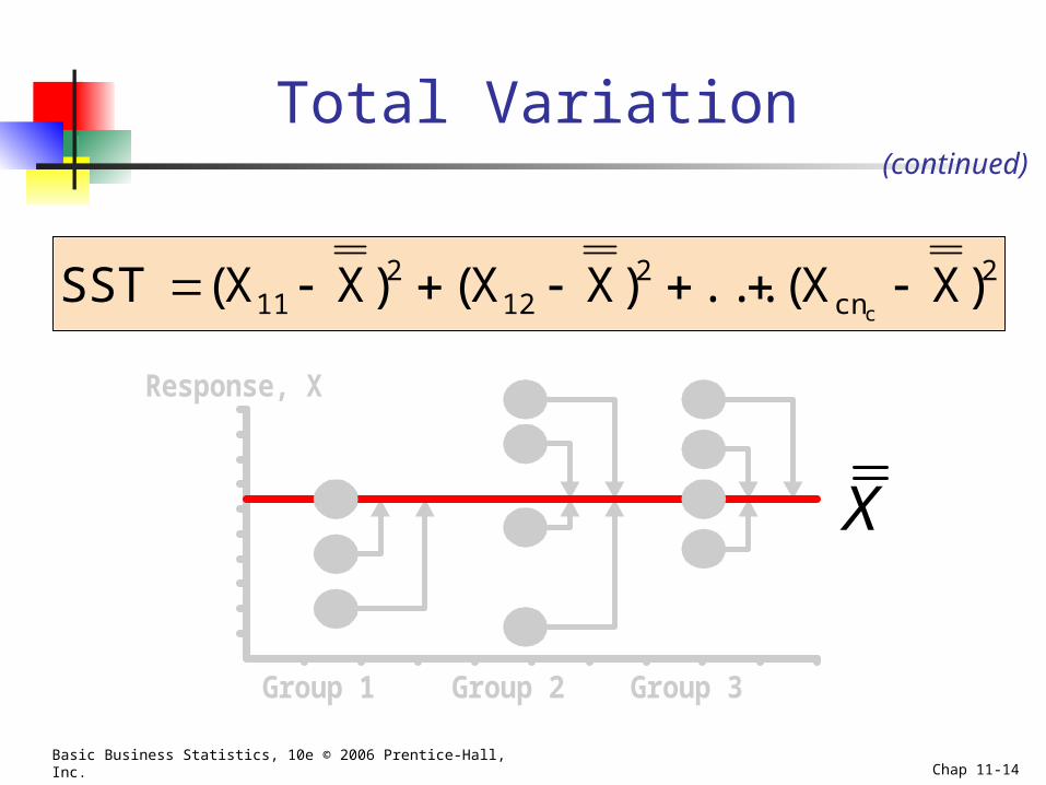
Total Variation
Group 1 Group 2 Group 3
Response, X
X
2cn
212
211 )XX(...)XX()XX(SST
c
(continued)
Basic Business Statistics, 10e © 2006 Prentice-Hall, Inc. Chap 11-15
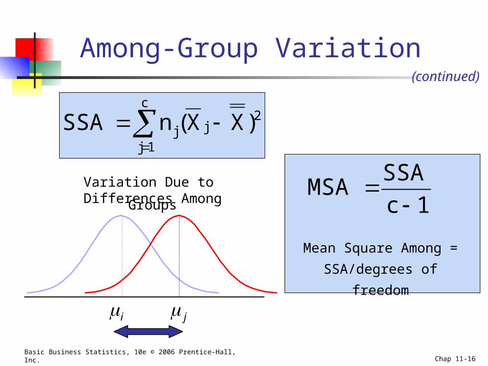
Among-Group Variation
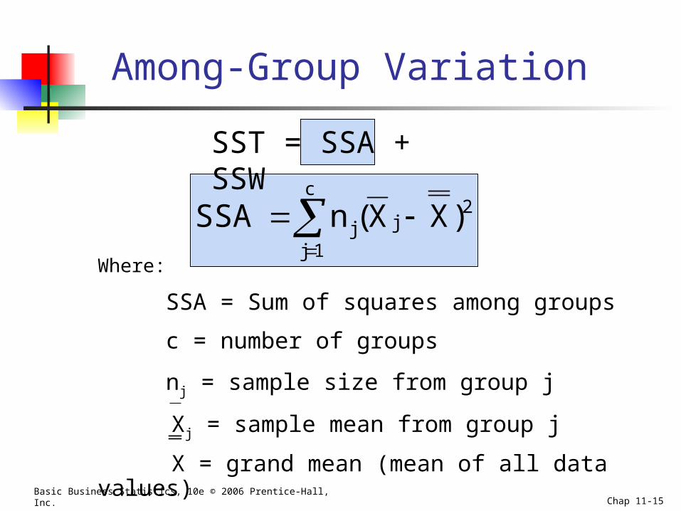
Where:
SSA = Sum of squares among groups
c = number of groups
nj = sample size from group j
Xj = sample mean from group j
X = grand mean (mean of all data values)
2j
c
1jj )XX(nSSA
SST = SSA + SSW
Basic Business Statistics, 10e © 2006 Prentice-Hall, Inc. Chap 11-16
Among-Group Variation
Variation Due to Differences Among Groups
i j
2j
c
1jj )XX(nSSA
1c
SSAMSA
Mean Square Among =
SSA/degrees of freedom
(continued)
Basic Business Statistics, 10e © 2006 Prentice-Hall, Inc. Chap 11-17
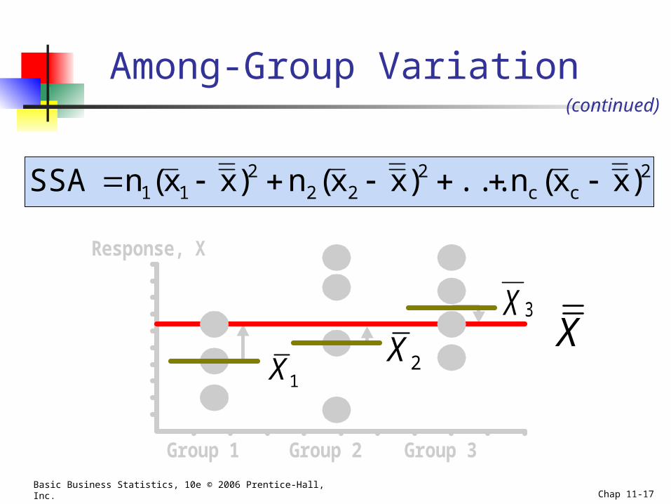
Among-Group Variation
Group 1 Group 2 Group 3
Response, X
X1X
2X3X
2222
211 )xx(n...)xx(n)xx(nSSA cc
(continued)
Basic Business Statistics, 10e © 2006 Prentice-Hall, Inc. Chap 11-18
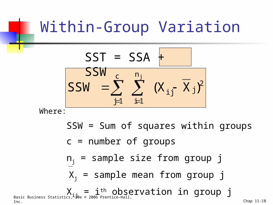
Within-Group Variation
Where:
SSW = Sum of squares within groups
c = number of groups
nj = sample size from group j
Xj = sample mean from group j
Xij = ith observation in group j
2jij
n
1i
c
1j
)XX(SSWj
SST = SSA + SSW
Basic Business Statistics, 10e © 2006 Prentice-Hall, Inc. Chap 11-19
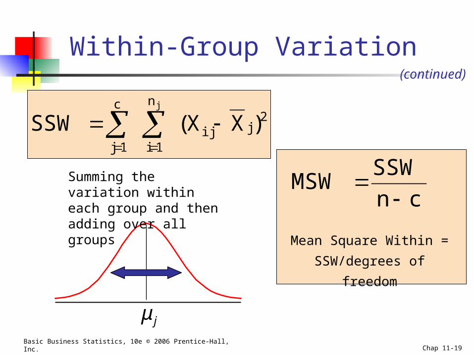
Within-Group Variation
Summing the variation within each group and then adding over all groups cn
SSWMSW
Mean Square Within =
SSW/degrees of freedom
2jij
n
1i
c
1j
)XX(SSWj
(continued)
jμ
Basic Business Statistics, 10e © 2006 Prentice-Hall, Inc. Chap 11-20
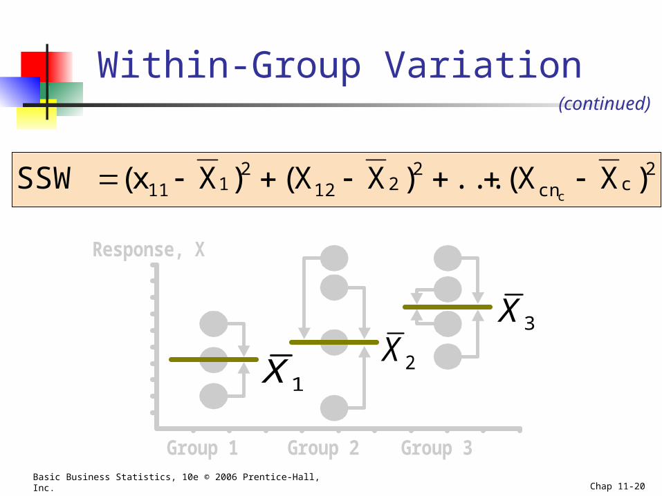
Within-Group Variation
Group 1 Group 2 Group 3
Response, X
1X2X
3X
2ccn
2212
2111 )XX(...)XX()Xx(SSW
c
(continued)
Basic Business Statistics, 10e © 2006 Prentice-Hall, Inc. Chap 11-21
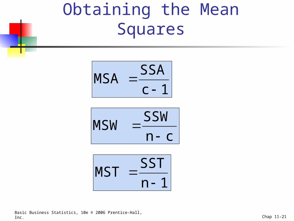
Obtaining the Mean Squares
cn
SSWMSW
1c
SSAMSA
1n
SSTMST
Basic Business Statistics, 10e © 2006 Prentice-Hall, Inc. Chap 11-22
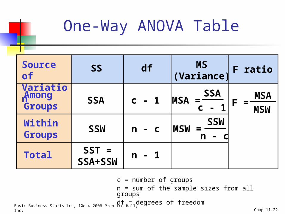
One-Way ANOVA Table
Source of Variation
dfSS MS(Variance)
Among Groups
SSA MSA =
Within Groups
n - cSSW MSW =
Total n - 1SST =SSA+SSW
c - 1 MSA
MSW
F ratio
c = number of groupsn = sum of the sample sizes from all groupsdf = degrees of freedom
SSA
c - 1
SSW
n - c
F =
Basic Business Statistics, 10e © 2006 Prentice-Hall, Inc. Chap 11-23
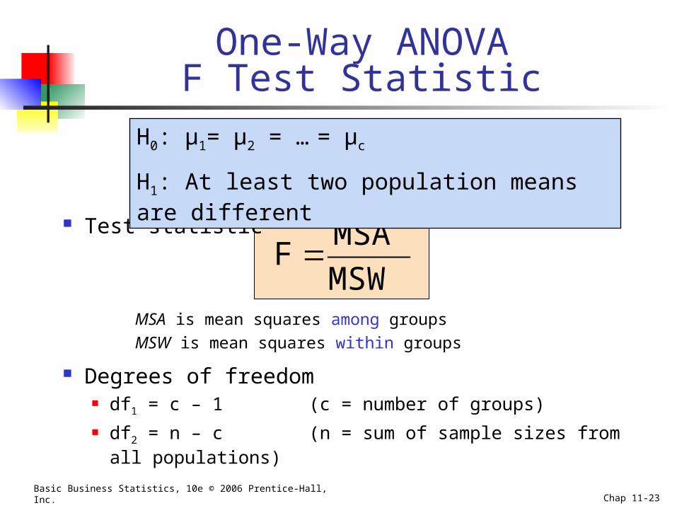
One-Way ANOVAF Test Statistic
Test statistic
MSA is mean squares among groups
MSW is mean squares within groups
Degrees of freedom df1 = c – 1 (c = number of groups)
df2 = n – c (n = sum of sample sizes from all populations)
MSW
MSAF
H0: μ1= μ2 = … = μc
H1: At least two population means are different
Basic Business Statistics, 10e © 2006 Prentice-Hall, Inc. Chap 11-24
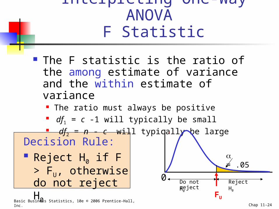
Interpreting One-Way ANOVA F Statistic
The F statistic is the ratio of the among estimate of variance and the within estimate of variance The ratio must always be positive df1 = c -1 will typically be small df2 = n - c will typically be large
Decision Rule: Reject H0 if F > FU,
otherwise do not reject H0
0
= .05
Reject H0Do not reject H0
FU
Basic Business Statistics, 10e © 2006 Prentice-Hall, Inc. Chap 11-25
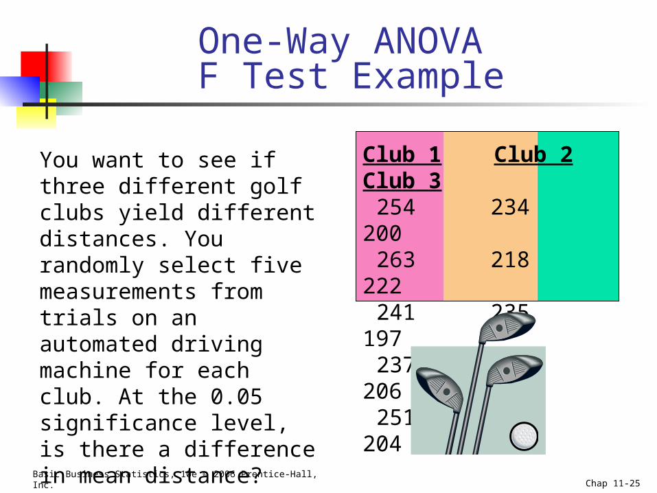
One-Way ANOVA F Test Example
You want to see if three different golf clubs yield different distances. You randomly select five measurements from trials on an automated driving machine for each club. At the 0.05 significance level, is there a difference in mean distance?
Club 1 Club 2 Club 3254 234 200263 218 222241 235 197237 227 206251 216 204
Basic Business Statistics, 10e © 2006 Prentice-Hall, Inc. Chap 11-26
••••
•
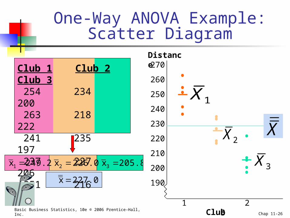
One-Way ANOVA Example: Scatter Diagram
270
260
250
240
230
220
210
200
190
••
•••
•••••
Distance
1X
2X
3X
X
227.0 x
205.8 x 226.0x 249.2x 321
Club 1 Club 2 Club 3254 234 200263 218 222241 235 197237 227 206251 216 204
Club1 2 3
Basic Business Statistics, 10e © 2006 Prentice-Hall, Inc. Chap 11-27
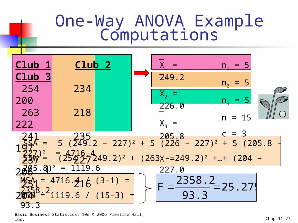
One-Way ANOVA Example Computations
Club 1 Club 2 Club 3254 234 200263 218 222241 235 197237 227 206251 216 204
X1 = 249.2
X2 = 226.0
X3 = 205.8
X = 227.0
n1 = 5
n2 = 5
n3 = 5
n = 15
c = 3SSA = 5 (249.2 – 227)2 + 5 (226 – 227)2 + 5 (205.8 – 227)2 = 4716.4
SSW = (254 – 249.2)2 + (263 – 249.2)2 +…+ (204 – 205.8)2 = 1119.6
MSA = 4716.4 / (3-1) = 2358.2
MSW = 1119.6 / (15-3) = 93.325.275
93.3
2358.2F
Basic Business Statistics, 10e © 2006 Prentice-Hall, Inc. Chap 11-28
F = 25.275
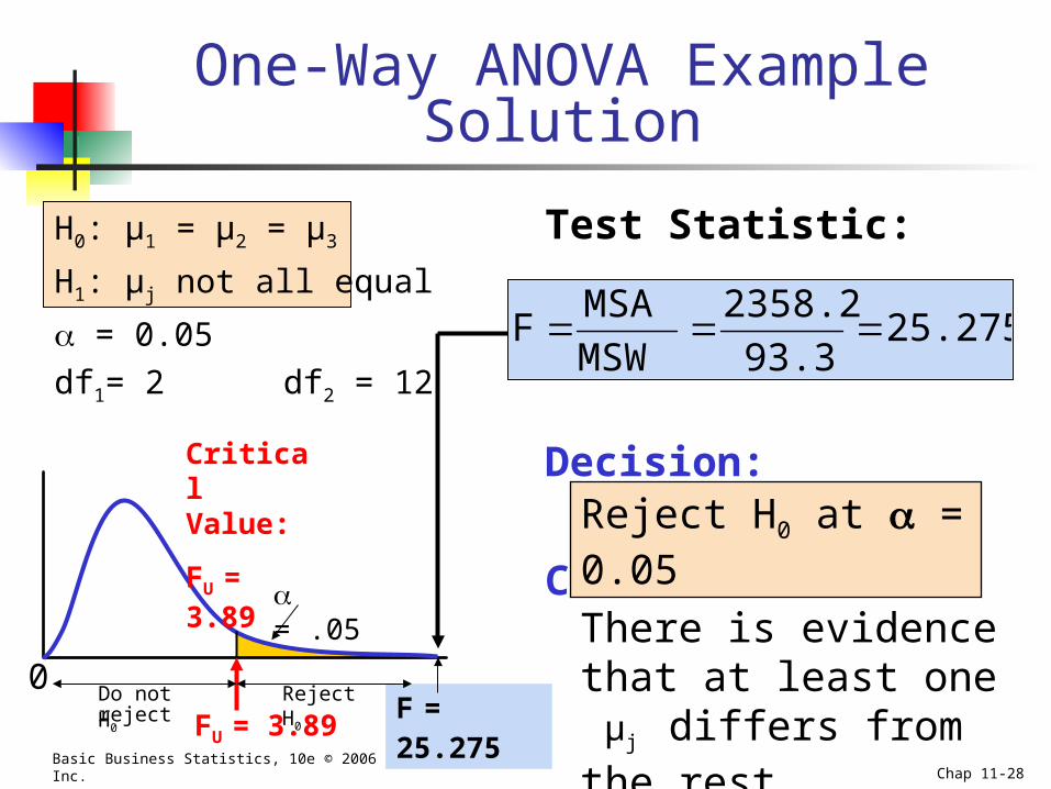
One-Way ANOVA Example Solution
H0: μ1 = μ2 = μ3
H1: μj not all equal
= 0.05
df1= 2 df2 = 12
Test Statistic:
Decision:
Conclusion:
Reject H0 at = 0.05
There is evidence that at least one μj differs from the rest
0
= .05
FU = 3.89Reject H0Do not
reject H0
25.27593.3
2358.2
MSW
MSAF
Critical Value:
FU = 3.89
Basic Business Statistics, 10e © 2006 Prentice-Hall, Inc. Chap 11-29
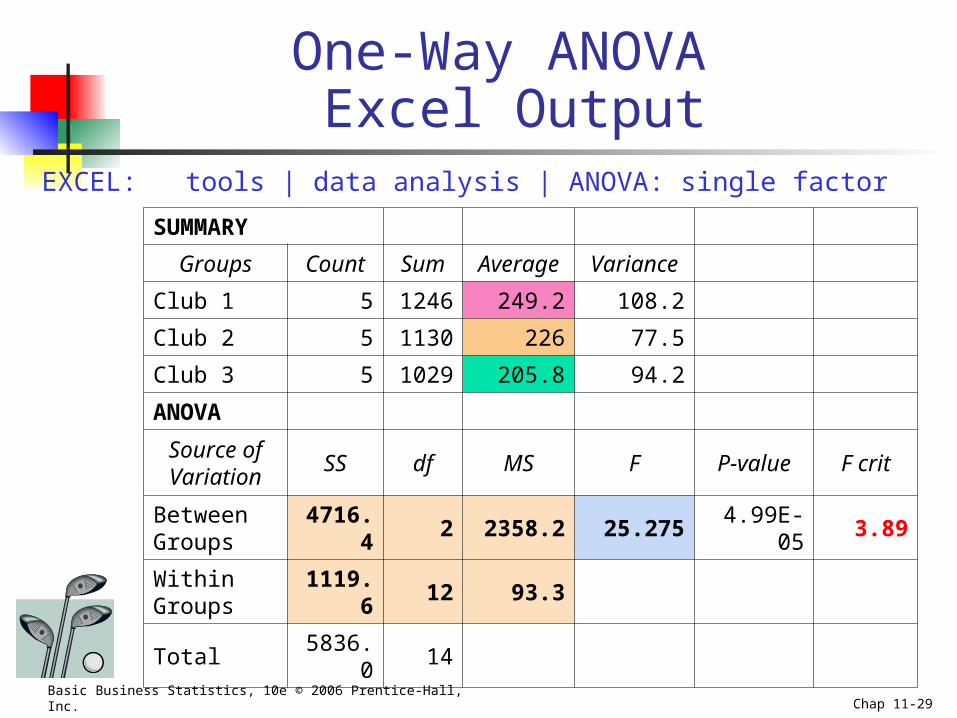
SUMMARY
Groups Count Sum Average Variance
Club 1 5 1246 249.2 108.2
Club 2 5 1130 226 77.5
Club 3 5 1029 205.8 94.2
ANOVA
Source of Variation
SS df MS F P-value F crit
Between Groups
4716.4 2 2358.2 25.275 4.99E-05 3.89
Within Groups
1119.6 12 93.3
Total 5836.0 14
One-Way ANOVA Excel Output
EXCEL: tools | data analysis | ANOVA: single factor
Basic Business Statistics, 10e © 2006 Prentice-Hall, Inc. Chap 11-30
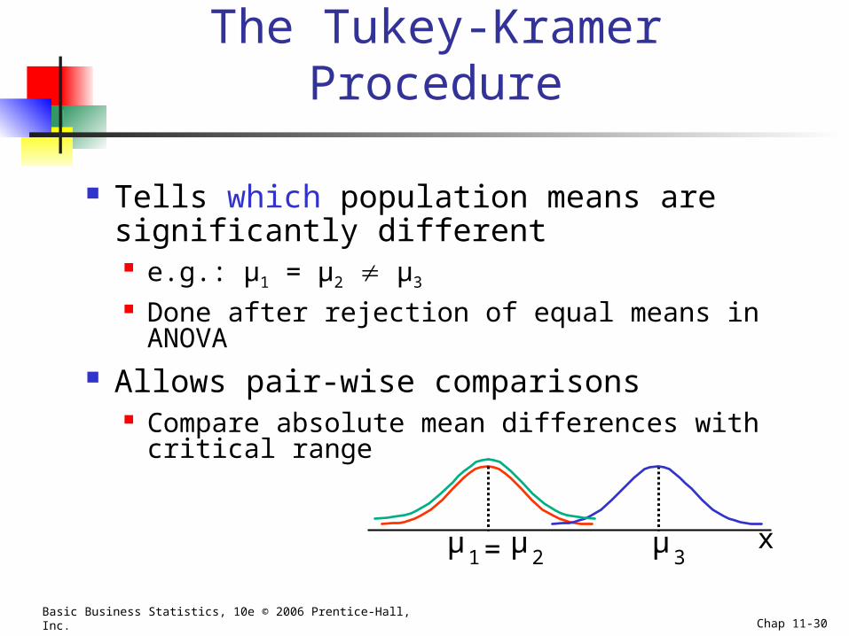
The Tukey-Kramer Procedure
Tells which population means are significantly different e.g.: μ1 = μ2 μ3
Done after rejection of equal means in ANOVA Allows pair-wise comparisons
Compare absolute mean differences with critical range
xμ1 = μ 2
μ3
Basic Business Statistics, 10e © 2006 Prentice-Hall, Inc. Chap 11-31
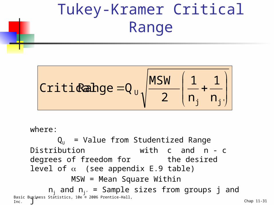
Tukey-Kramer Critical Range
where:QU = Value from Studentized Range Distribution
with c and n - c degrees of freedom for the desired level of (see appendix E.9 table)
MSW = Mean Square Within nj and nj’ = Sample sizes from groups j and j’
j'jU n
1
n
1
2
MSWQRange Critical
Basic Business Statistics, 10e © 2006 Prentice-Hall, Inc. Chap 11-32
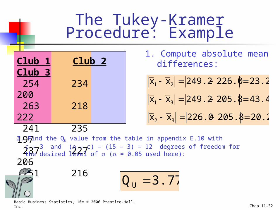
The Tukey-Kramer Procedure: Example
1. Compute absolute mean differences:Club 1 Club 2 Club 3
254 234 200263 218 222241 235 197237 227 206251 216 204 20.2205.8226.0xx
43.4205.8249.2xx
23.2226.0249.2xx
32
31
21
2. Find the QU value from the table in appendix E.10 with c = 3 and (n – c) = (15 – 3) = 12 degrees of freedom for the desired level of ( = 0.05 used here):
3.77QU
Basic Business Statistics, 10e © 2006 Prentice-Hall, Inc. Chap 11-33
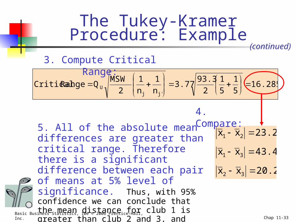
The Tukey-Kramer Procedure: Example
5. All of the absolute mean differences are greater than critical range. Therefore there is a significant difference between each pair of means at 5% level of significance. Thus, with 95% confidence we can conclude that the mean distance for club 1 is greater than club 2 and 3, and club 2 is greater than club 3.
16.2855
1
5
1
2
93.33.77
n
1
n
1
2
MSWQRange Critical
j'jU
3. Compute Critical Range:
20.2xx
43.4xx
23.2xx
32
31
21
4. Compare:
(continued)
Basic Business Statistics, 10e © 2006 Prentice-Hall, Inc. Chap 11-34
The Randomized Block Design
Like One-Way ANOVA, we test for equal population means (for different factor levels, for example)...
...but we want to control for possible variation from a second factor (with two or more levels)
Levels of the secondary factor are called blocks
Basic Business Statistics, 10e © 2006 Prentice-Hall, Inc. Chap 11-35
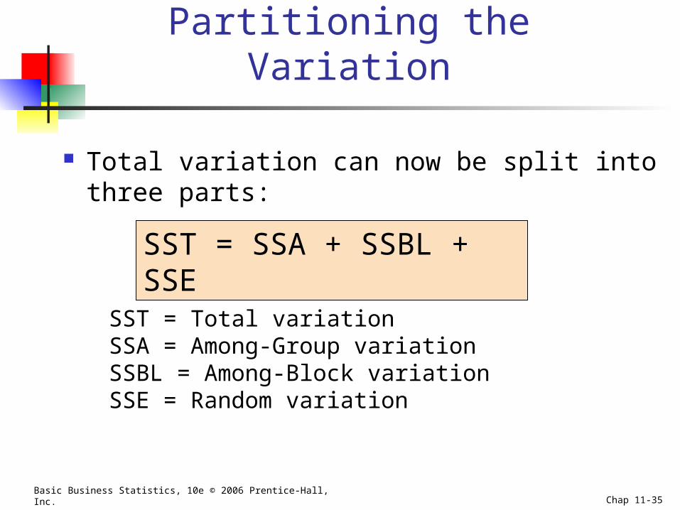
Partitioning the Variation
Total variation can now be split into three parts:
SST = Total variationSSA = Among-Group variationSSBL = Among-Block variationSSE = Random variation
SST = SSA + SSBL + SSE
Basic Business Statistics, 10e © 2006 Prentice-Hall, Inc. Chap 11-36
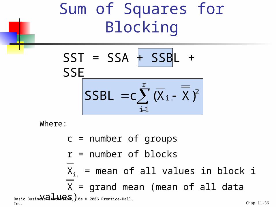
Sum of Squares for Blocking
Where:
c = number of groups
r = number of blocks
Xi. = mean of all values in block i
X = grand mean (mean of all data values)
r
1i
2i. )XX(cSSBL
SST = SSA + SSBL + SSE

Basic Business Statistics, 10e © 2006 Prentice-Hall, Inc. Chap 11-37
Partitioning the Variation
Total variation can now be split into three parts:
SST and SSA are computed as they were in One-Way ANOVA
SST = SSA + SSBL + SSE
SSE = SST – (SSA + SSBL)
Basic Business Statistics, 10e © 2006 Prentice-Hall, Inc. Chap 11-38
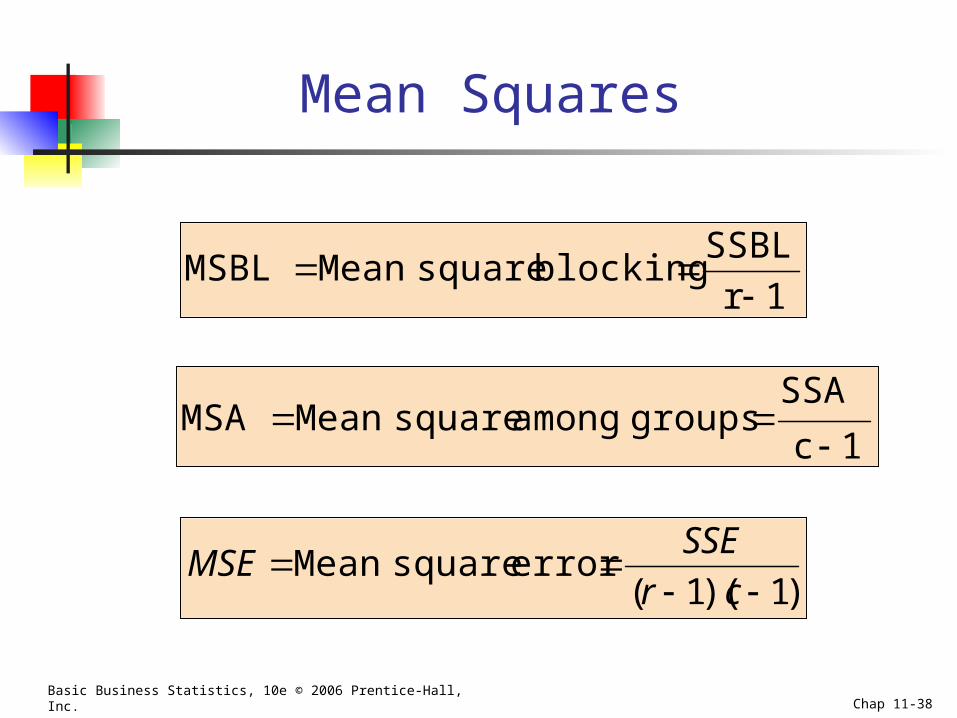
Mean Squares
1c
SSAgroups among square MeanMSA
1r
SSBLblocking square MeanMSBL
)1)(1(
cr
SSEMSE error square Mean
Basic Business Statistics, 10e © 2006 Prentice-Hall, Inc. Chap 11-39
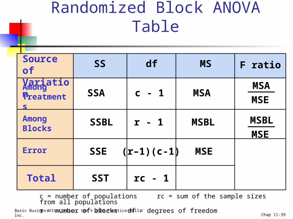
Randomized Block ANOVA Table
Source of Variation
dfSS MS
Among Blocks
SSBL MSBL
Error (r–1)(c-1)SSE MSE
Total rc - 1SST
r - 1 MSBL
MSE
F ratio
c = number of populations rc = sum of the sample sizes from all populationsr = number of blocks df = degrees of freedom
Among Treatments SSA c - 1 MSA
MSA
MSE
Basic Business Statistics, 10e © 2006 Prentice-Hall, Inc. Chap 11-40
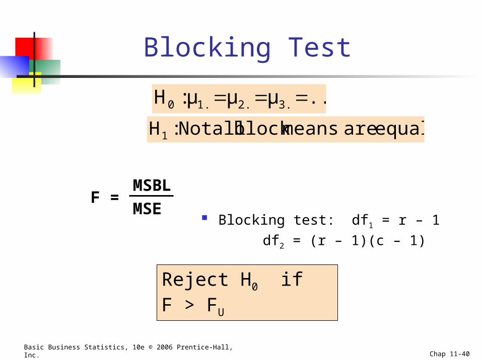
Blocking Test
Blocking test: df1 = r – 1
df2 = (r – 1)(c – 1)
MSBL
MSE
...μμμ:H 3.2.1.0
equal are means block all Not:H1
F =
Reject H0 if F > FU
Basic Business Statistics, 10e © 2006 Prentice-Hall, Inc. Chap 11-41
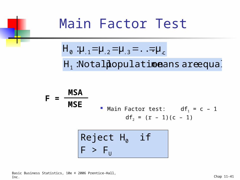
Main Factor test: df1 = c – 1
df2 = (r – 1)(c – 1)
MSA
MSE
c..3.2.10 μ...μμμ:H
equal are means population all Not:H1
F =
Reject H0 if F > FU
Main Factor Test
Basic Business Statistics, 10e © 2006 Prentice-Hall, Inc. Chap 11-42
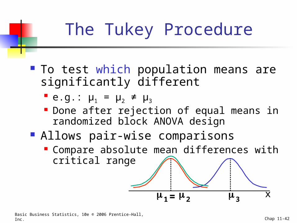
The Tukey Procedure
To test which population means are significantly different e.g.: μ1 = μ2 ≠ μ3
Done after rejection of equal means in randomized block ANOVA design
Allows pair-wise comparisons Compare absolute mean differences with critical
range
x = 1 2 3
Basic Business Statistics, 10e © 2006 Prentice-Hall, Inc. Chap 11-43
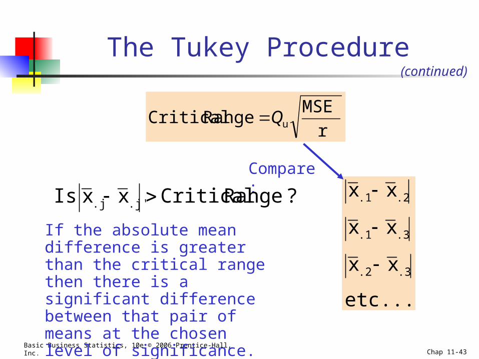
etc...
xx
xx
xx
.3.2
.3.1
.2.1
The Tukey Procedure(continued)
r
MSERange Critical uQ
If the absolute mean difference is greater than the critical range then there is a significant difference between that pair of means at the chosen level of significance.
Compare:
?Range CriticalxxIs .j'.j
Basic Business Statistics, 10e © 2006 Prentice-Hall, Inc. Chap 11-44
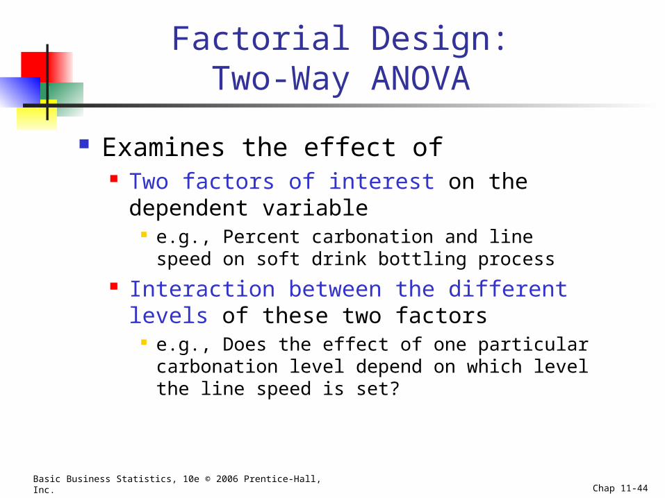
Factorial Design:Two-Way ANOVA
Examines the effect of Two factors of interest on the dependent
variable e.g., Percent carbonation and line speed on soft drink
bottling process Interaction between the different levels of these
two factors e.g., Does the effect of one particular carbonation
level depend on which level the line speed is set?
Basic Business Statistics, 10e © 2006 Prentice-Hall, Inc. Chap 11-45
Two-Way ANOVA
Assumptions
Populations are normally distributed
Populations have equal variances
Independent random samples are drawn
(continued)
Basic Business Statistics, 10e © 2006 Prentice-Hall, Inc. Chap 11-46
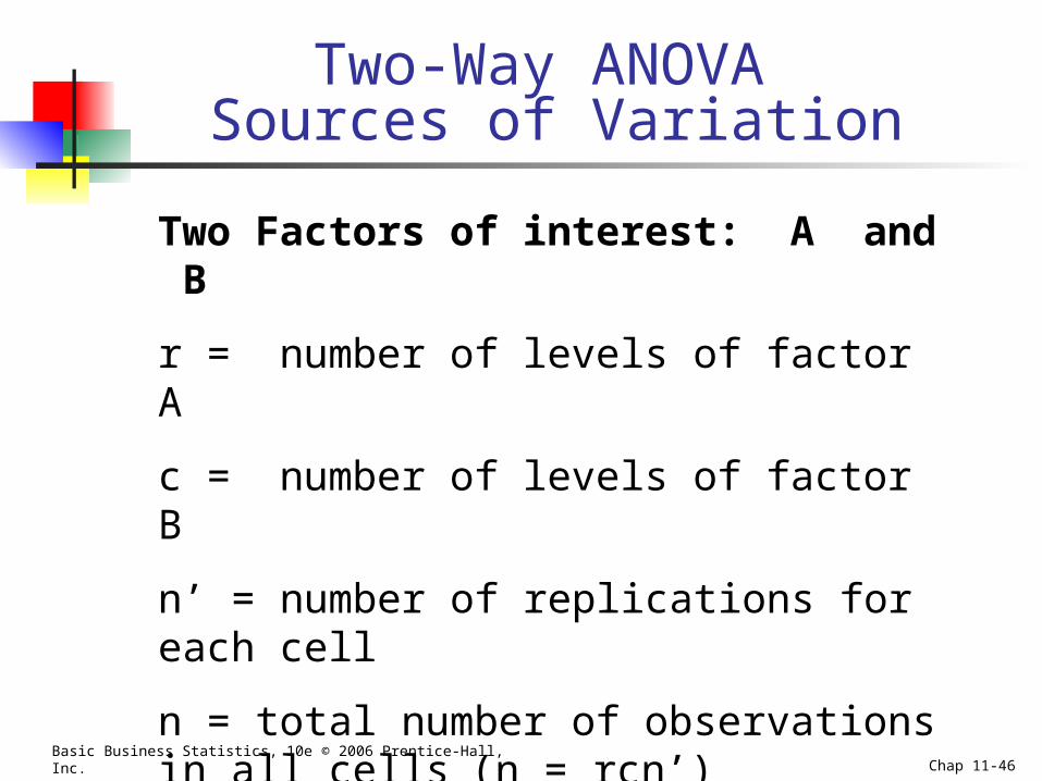
Two-Way ANOVA Sources of Variation
Two Factors of interest: A and B
r = number of levels of factor A
c = number of levels of factor B
n’ = number of replications for each cell
n = total number of observations in all cells(n = rcn’)
Xijk = value of the kth observation of level i of factor A and level j of factor B
Basic Business Statistics, 10e © 2006 Prentice-Hall, Inc. Chap 11-47
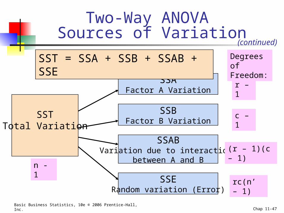
Two-Way ANOVA Sources of Variation
SSTTotal Variation
SSAFactor A Variation
SSBFactor B Variation
SSABVariation due to interaction
between A and B
SSERandom variation (Error)
Degrees of Freedom:
r – 1
c – 1
(r – 1)(c – 1)
rc(n’ – 1)
n - 1
SST = SSA + SSB + SSAB + SSE
(continued)
Basic Business Statistics, 10e © 2006 Prentice-Hall, Inc. Chap 11-48
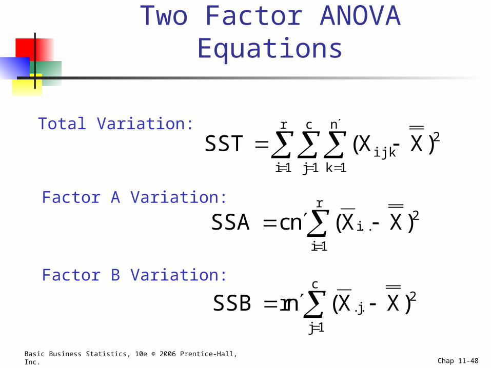
Two Factor ANOVA Equations
r
1i
c
1j
n
1k
2ijk )XX(SST
2r
1i
..i )XX(ncSSA
2c
1j
.j. )XX(nrSSB
Total Variation:
Factor A Variation:
Factor B Variation:
Basic Business Statistics, 10e © 2006 Prentice-Hall, Inc. Chap 11-49
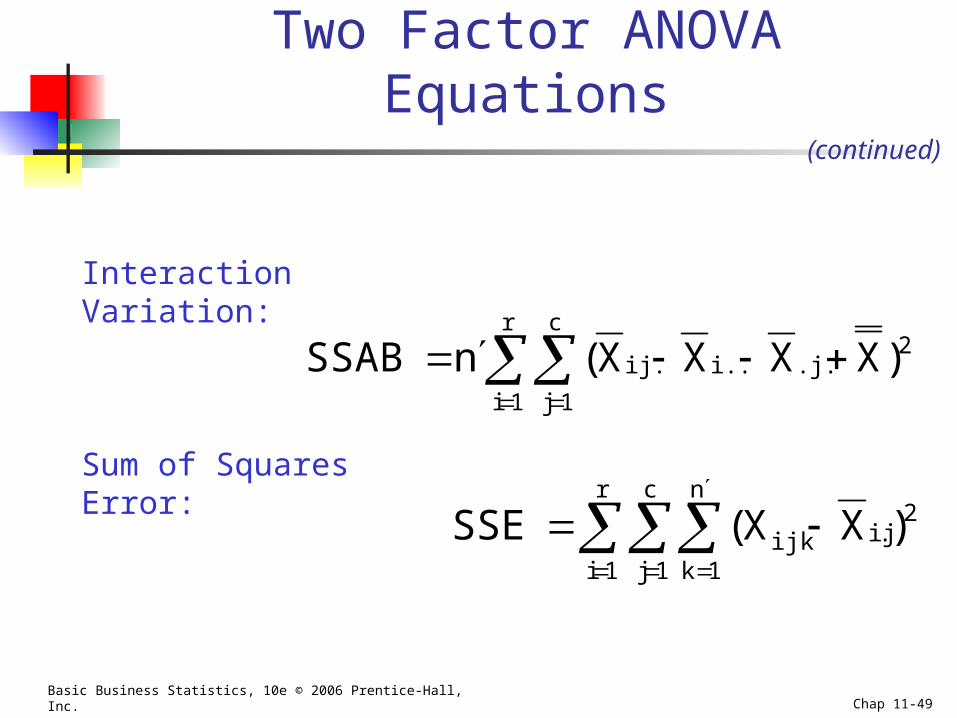
Two Factor ANOVA Equations
2r
1i
c
1j
.j.i..ij. )XXXX(nSSAB
r
1i
c
1j
n
1k
2.ijijk )XX(SSE
Interaction Variation:
Sum of Squares Error:
(continued)
Basic Business Statistics, 10e © 2006 Prentice-Hall, Inc. Chap 11-50
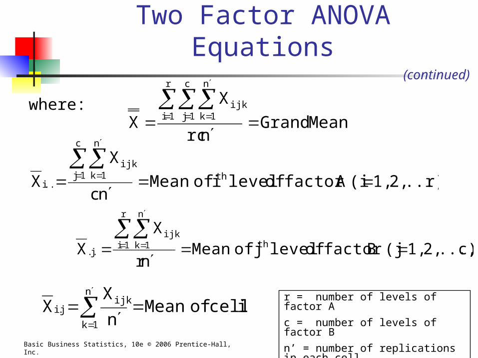
Two Factor ANOVA Equations
where:Mean Grand
nrc
X
X
r
1i
c
1j
n
1kijk
r) ..., 2, 1, (i A factor of level i of Meannc
X
X th
c
1j
n
1kijk
..i
c) ..., 2, 1, (j B factor of level j of Meannr
XX th
r
1i
n
1kijk
.j.
ij cell of Meann
XX
n
1k
ijk.ij
r = number of levels of factor A
c = number of levels of factor B
n’ = number of replications in each cell
(continued)
Basic Business Statistics, 10e © 2006 Prentice-Hall, Inc. Chap 11-51
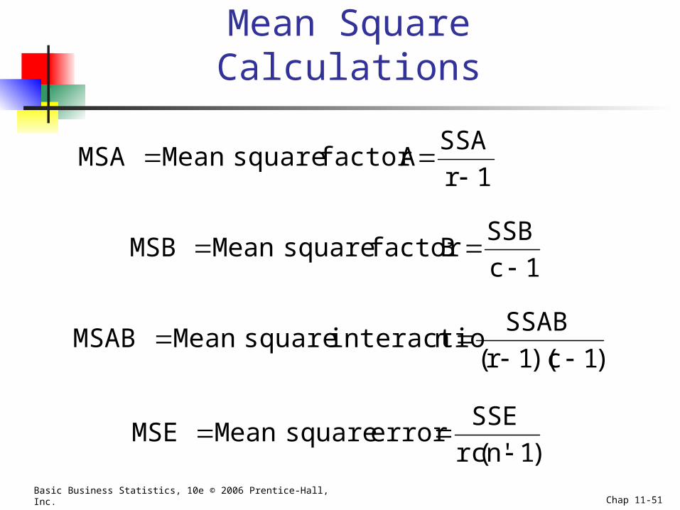
Mean Square Calculations
1r
SSA Afactor square MeanMSA
1c
SSBB factor square MeanMSB
)1c)(1r(
SSABninteractio square MeanMSAB
)1'n(rc
SSEerror square MeanMSE
Basic Business Statistics, 10e © 2006 Prentice-Hall, Inc. Chap 11-52
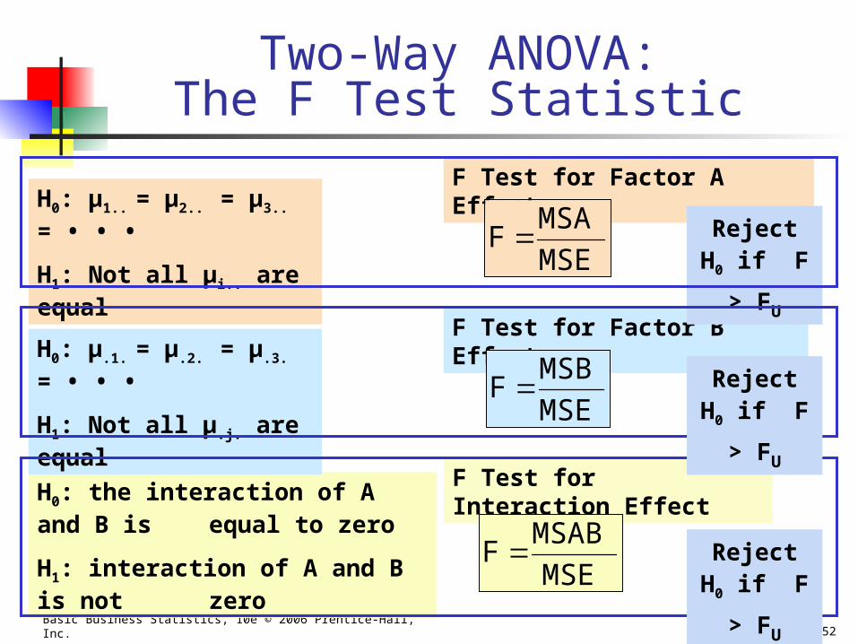
Two-Way ANOVA:The F Test Statistic
F Test for Factor B Effect
F Test for Interaction Effect
H0: μ1.. = μ2.. = μ3.. = • • •
H1: Not all μi.. are equal
H0: the interaction of A and B is equal to zero
H1: interaction of A and B is not zero
F Test for Factor A Effect
H0: μ.1. = μ.2. = μ.3. = • • •
H1: Not all μ.j. are equal
Reject H0
if F > FUMSE
MSAF
MSE
MSBF
MSE
MSABF
Reject H0
if F > FU
Reject H0
if F > FU
Basic Business Statistics, 10e © 2006 Prentice-Hall, Inc. Chap 11-53
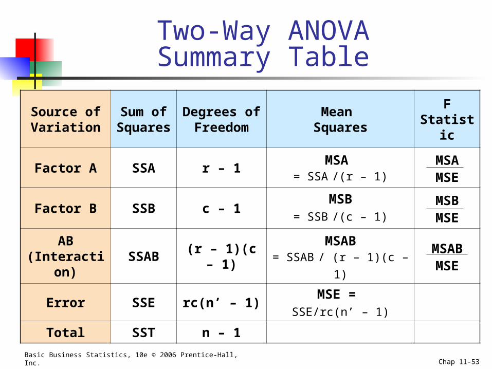
Two-Way ANOVASummary Table
Source ofVariation
Sum ofSquares
Degrees of Freedom
Mean Squares
FStatistic
Factor A SSA r – 1MSA
= SSA /(r – 1)MSAMSE
Factor B SSB c – 1MSB
= SSB /(c – 1)MSBMSE
AB(Interaction)
SSAB (r – 1)(c – 1)MSAB
= SSAB / (r – 1)(c – 1)MSABMSE
Error SSE rc(n’ – 1)MSE =
SSE/rc(n’ – 1)
Total SST n – 1
Basic Business Statistics, 10e © 2006 Prentice-Hall, Inc. Chap 11-54
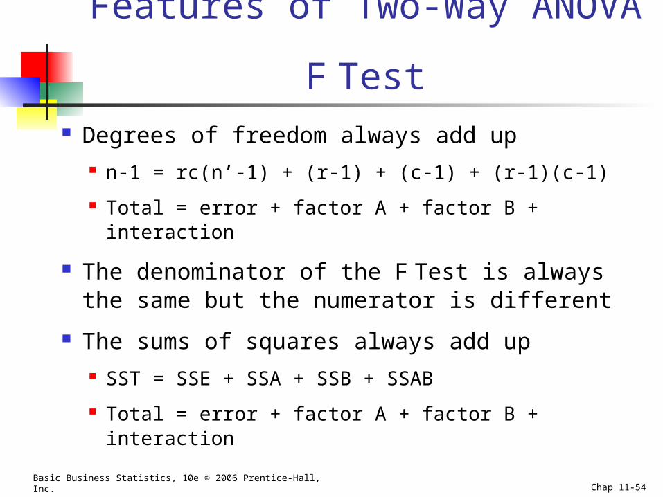
Features of Two-Way ANOVA F Test
Degrees of freedom always add up n-1 = rc(n’-1) + (r-1) + (c-1) + (r-1)(c-1)
Total = error + factor A + factor B + interaction
The denominator of the F Test is always the same but the numerator is different
The sums of squares always add up SST = SSE + SSA + SSB + SSAB
Total = error + factor A + factor B + interaction
Basic Business Statistics, 10e © 2006 Prentice-Hall, Inc. Chap 11-55
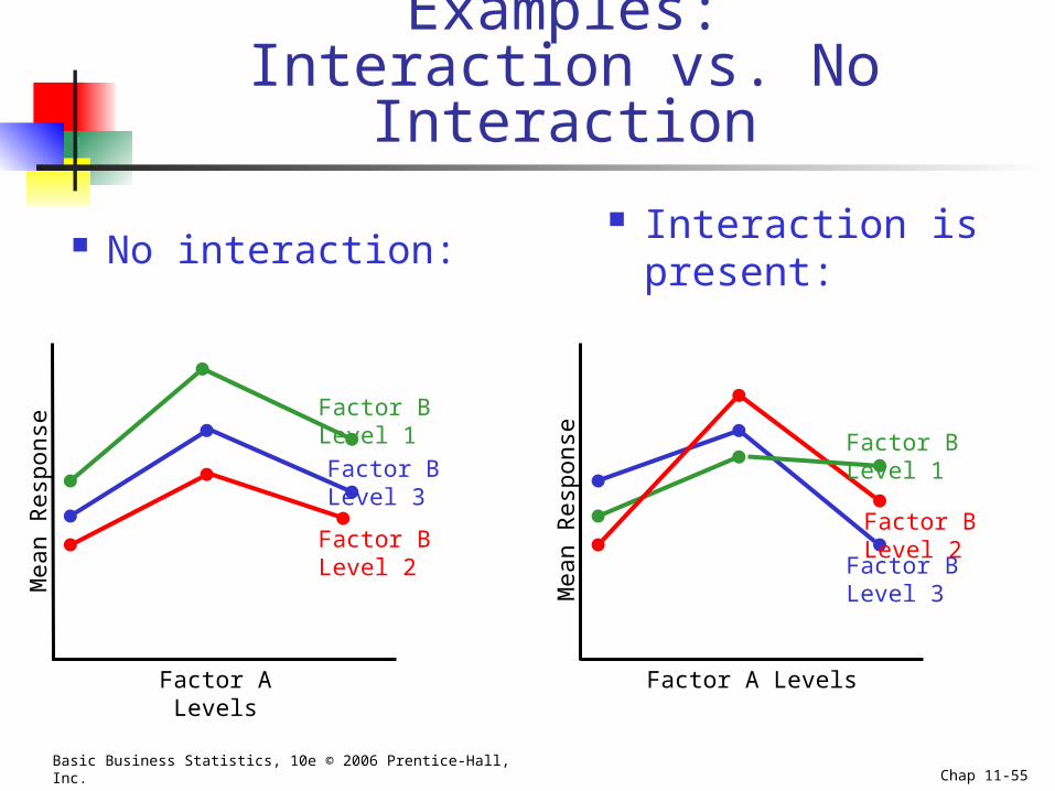
Examples:Interaction vs. No Interaction
No interaction:
Factor B Level 1
Factor B Level 3
Factor B Level 2
Factor A Levels
Factor B Level 1
Factor B Level 3
Factor B Level 2
Factor A Levels
Mea
n R
espo
nse
Mea
n R
espo
nse
Interaction is present:
Basic Business Statistics, 10e © 2006 Prentice-Hall, Inc. Chap 11-56
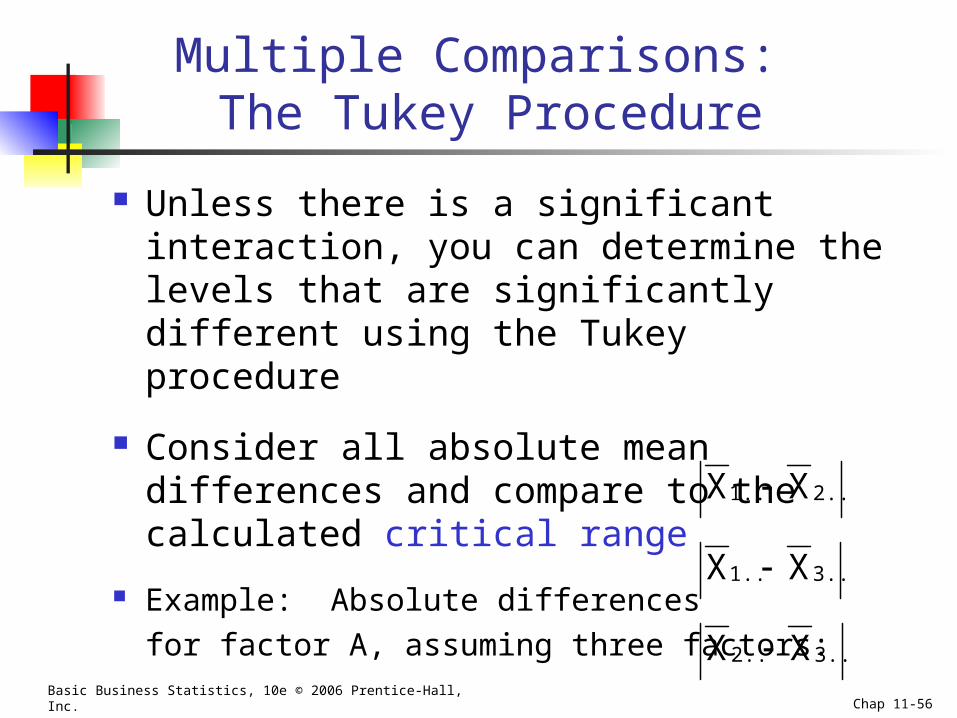
Multiple Comparisons: The Tukey Procedure
Unless there is a significant interaction, you can determine the levels that are significantly different using the Tukey procedure
Consider all absolute mean differences and compare to the calculated critical range
Example: Absolute differences
for factor A, assuming three factors:
3..2..
3..1..
2..1..
XX
XX
XX
Basic Business Statistics, 10e © 2006 Prentice-Hall, Inc. Chap 11-57
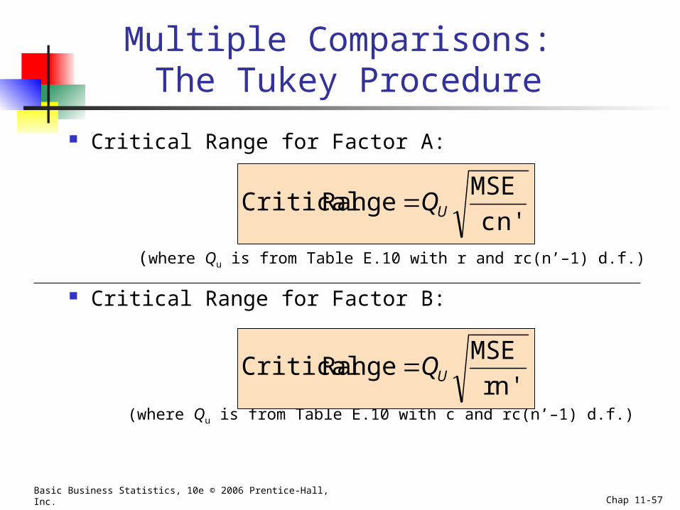
Multiple Comparisons: The Tukey Procedure
Critical Range for Factor A:
(where Qu is from Table E.10 with r and rc(n’–1) d.f.)
Critical Range for Factor B:
(where Qu is from Table E.10 with c and rc(n’–1) d.f.)
n'c
MSERange Critical UQ
n'r
MSERange Critical UQ
Basic Business Statistics, 10e © 2006 Prentice-Hall, Inc. Chap 11-58
Chapter Summary
Described one-way analysis of variance The logic of ANOVA ANOVA assumptions F test for difference in c means The Tukey-Kramer procedure for multiple comparisons
Considered the Randomized Block Design Treatment and Block Effects Multiple Comparisons: Tukey Procedure
Described two-way analysis of variance Examined effects of multiple factors Examined interaction between factors