Embed Size (px)
Citation preview
Basic Business Statistics, 10e © 2006 Prentice-Hall, Inc.. Chap 5-1
Chapter 5
Some Important Discrete Probability Distributions
Basic Business Statistics10th Edition
Basic Business Statistics, 10e © 2006 Prentice-Hall, Inc. Chap 5-2
Learning Objectives
In this chapter, you learn: The properties of a probability distribution To calculate the expected value and variance of a
probability distribution To calculate the covariance and its use in finance To calculate probabilities from binomial, Poisson
distributions and hypergeometric How to use the binomial, hypergeometric, and
Poisson distributions to solve business problems
Basic Business Statistics, 10e © 2006 Prentice-Hall, Inc. Chap 5-3
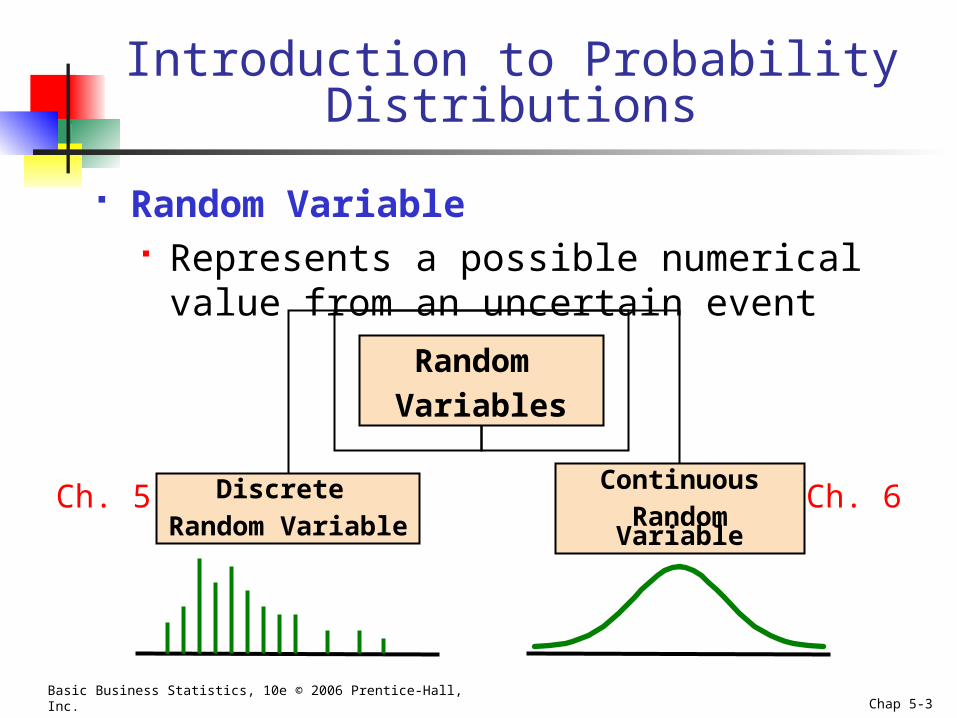
Introduction to Probability Distributions
Random Variable Represents a possible numerical value from
an uncertain event
Random
Variables
Discrete Random Variable
ContinuousRandom Variable
Ch. 5 Ch. 6
Basic Business Statistics, 10e © 2006 Prentice-Hall, Inc. Chap 5-4
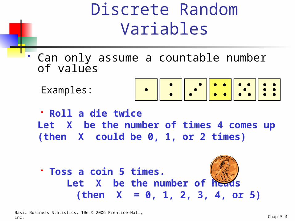
Discrete Random Variables
Can only assume a countable number of values
Examples:
Roll a die twiceLet X be the number of times 4 comes up (then X could be 0, 1, or 2 times)
Toss a coin 5 times. Let X be the number of heads
(then X = 0, 1, 2, 3, 4, or 5)
Basic Business Statistics, 10e © 2006 Prentice-Hall, Inc. Chap 5-5
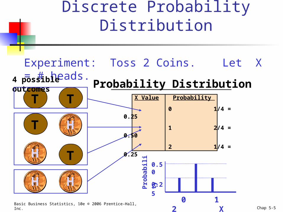
Experiment: Toss 2 Coins. Let X = # heads.
T
T
Discrete Probability Distribution
4 possible outcomes
T
T
H
H
H H
Probability Distribution
0 1 2 X
X Value Probability
0 1/4 = 0.25
1 2/4 = 0.50
2 1/4 = 0.25
0.50
0.25
Pro
bab
ility
Basic Business Statistics, 10e © 2006 Prentice-Hall, Inc. Chap 5-6
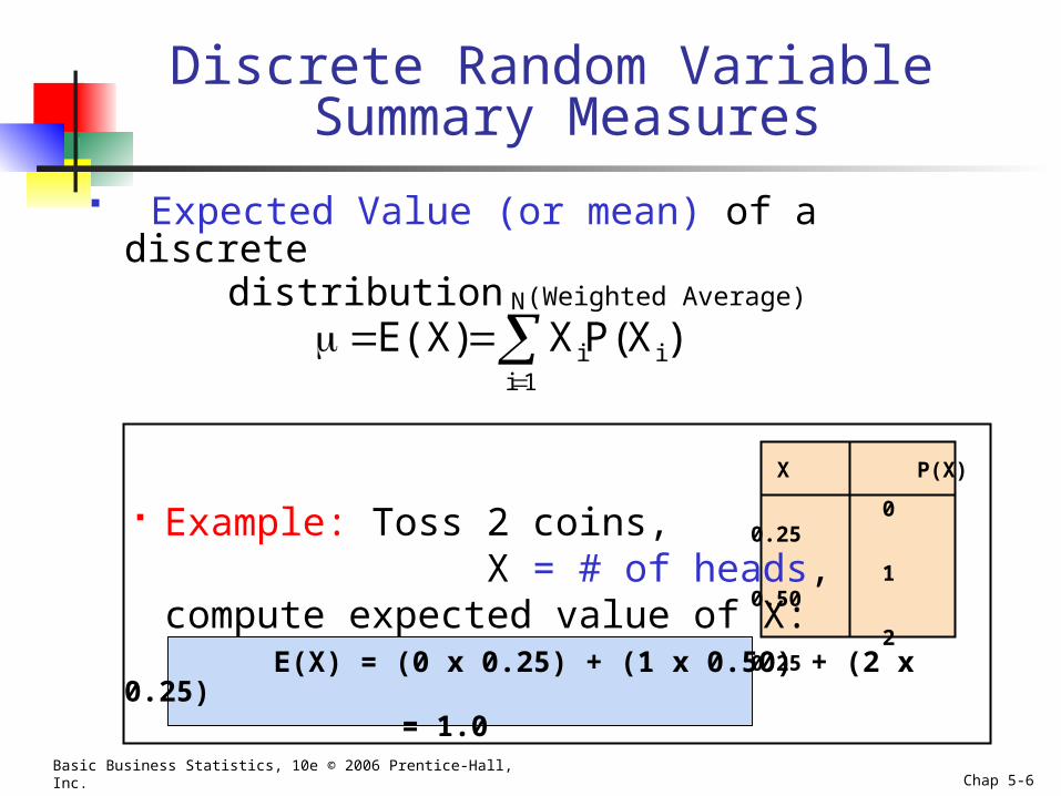
Discrete Random Variable Summary Measures
Expected Value (or mean) of a discrete distribution (Weighted Average)
Example: Toss 2 coins, X = # of heads, compute expected value of X:
E(X) = (0 x 0.25) + (1 x 0.50) + (2 x 0.25) = 1.0
X P(X)
0 0.25
1 0.50
2 0.25
N
1iii )X(PX E(X)
Basic Business Statistics, 10e © 2006 Prentice-Hall, Inc. Chap 5-7
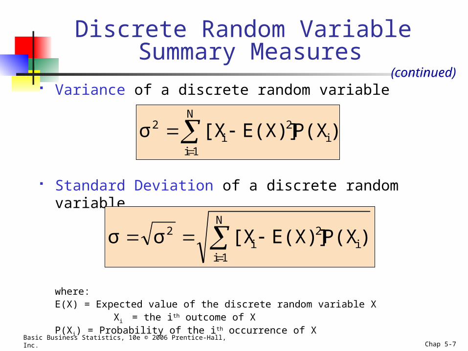
Variance of a discrete random variable
Standard Deviation of a discrete random variable
where:E(X) = Expected value of the discrete random variable X
Xi = the ith outcome of XP(Xi) = Probability of the ith occurrence of X
Discrete Random Variable Summary Measures
N
1ii
2i
2 )P(XE(X)][Xσ
(continued)
N
1ii
2i
2 )P(XE(X)][Xσσ
Basic Business Statistics, 10e © 2006 Prentice-Hall, Inc. Chap 5-8
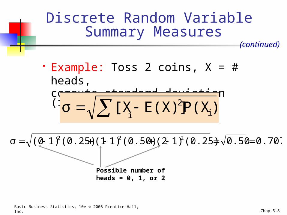
Example: Toss 2 coins, X = # heads, compute standard deviation (recall E(X) = 1)
Discrete Random Variable Summary Measures
)P(XE(X)][Xσ i2
i
0.7070.50(0.25)1)(2(0.50)1)(1(0.25)1)(0σ 222
(continued)
Possible number of heads = 0, 1, or 2

Basic Business Statistics, 10e © 2006 Prentice-Hall, Inc. Chap 5-9
二元隨機變數之機率分配
Basic Business Statistics, 10e © 2006 Prentice-Hall, Inc. Chap 5-10
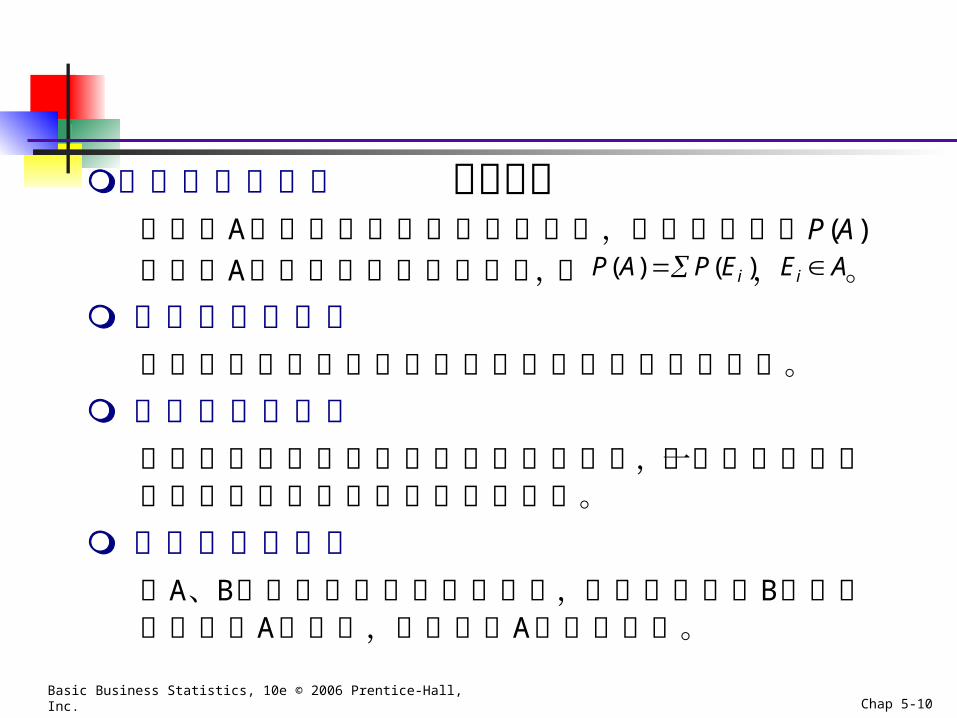
事件機率的定義
設事件A定義於隨機實驗的樣本空間,其發生之機率P(A)
為事件A之基本出象的機率總和,即 )()( iEPAP , AEi 。
聯合機率的定義
二個或二個以上事件同時發生的機率稱為聯合機率。
邊際機率的定義
在有二個或二個以上類別的樣本空間中,若僅考慮某一類別個別發生的機率者稱為邊際機率。
條件機率的定義
令A、B為定義於樣本空間的事件,已知發生事件B之後再發生事件A的機率,稱為事件A的條件機率。
事件機率
Basic Business Statistics, 10e © 2006 Prentice-Hall, Inc. Chap 5-11
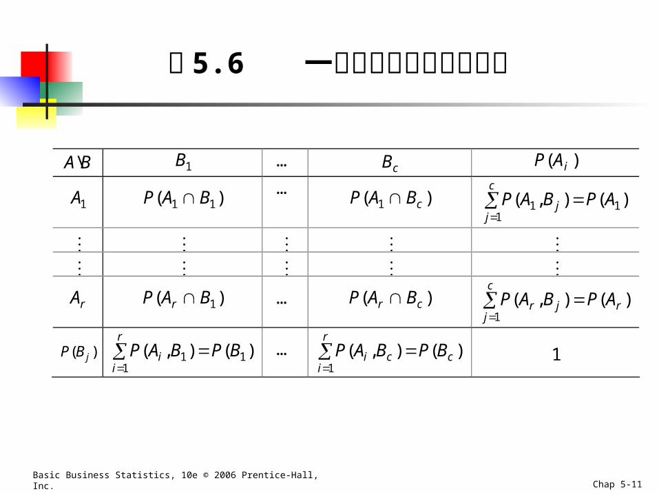
表 5.6 一般化的聯合機率分配表
A\B 1B … cB )( iAP
1A )( 11 BAP … )( 1 cBAP
c
jj APBAP
111 )(),(
rA )( 1BAP r … )( cr BAP
c
jrjr APBAP
1)(),(
)( jBP
r
ii BPBAP
111 )(),( …
r
icci BPBAP
1)(),( 1
Basic Business Statistics, 10e © 2006 Prentice-Hall, Inc. Chap 5-12
( ) ( ) ( , )
( , ) ( , )
( , ) ( , )
( ) ( )
( ) ( )
i j i ji j
i i j j i ji j i j
i i j j i ji j j i
i i j ji j
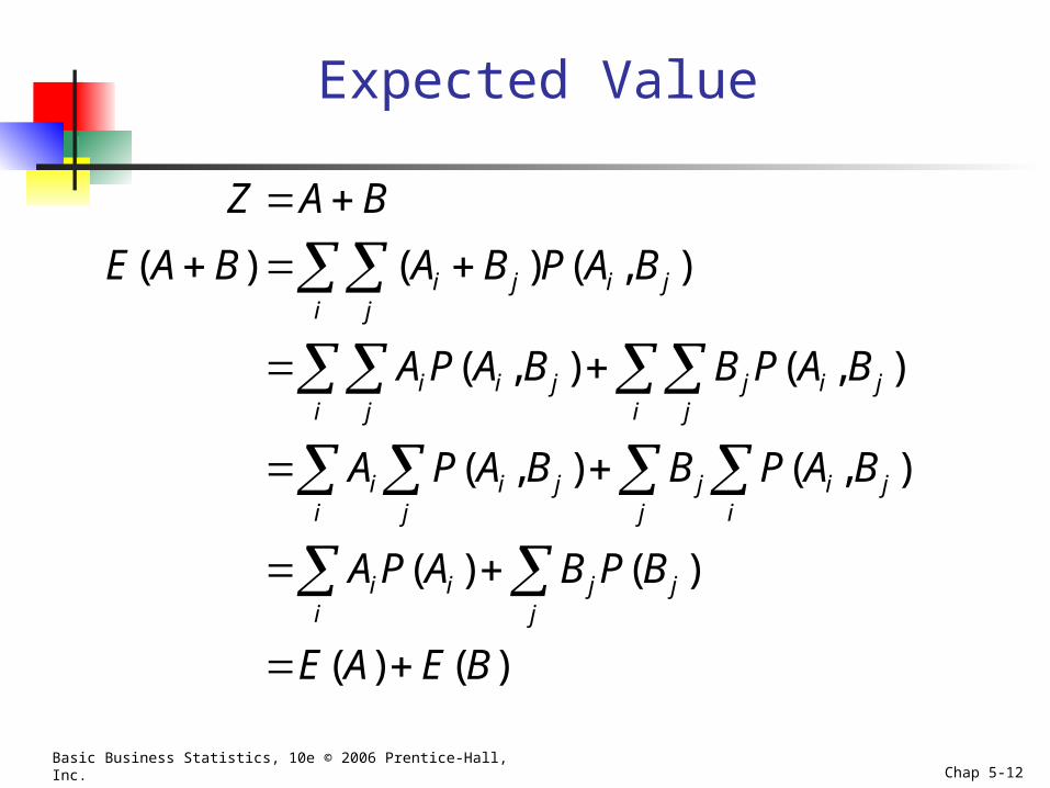
Z A B
E A B A B P A B
AP A B B P A B
A P A B B P A B
AP A B P B
E A E B
Expected Value
Basic Business Statistics, 10e © 2006 Prentice-Hall, Inc. Chap 5-13
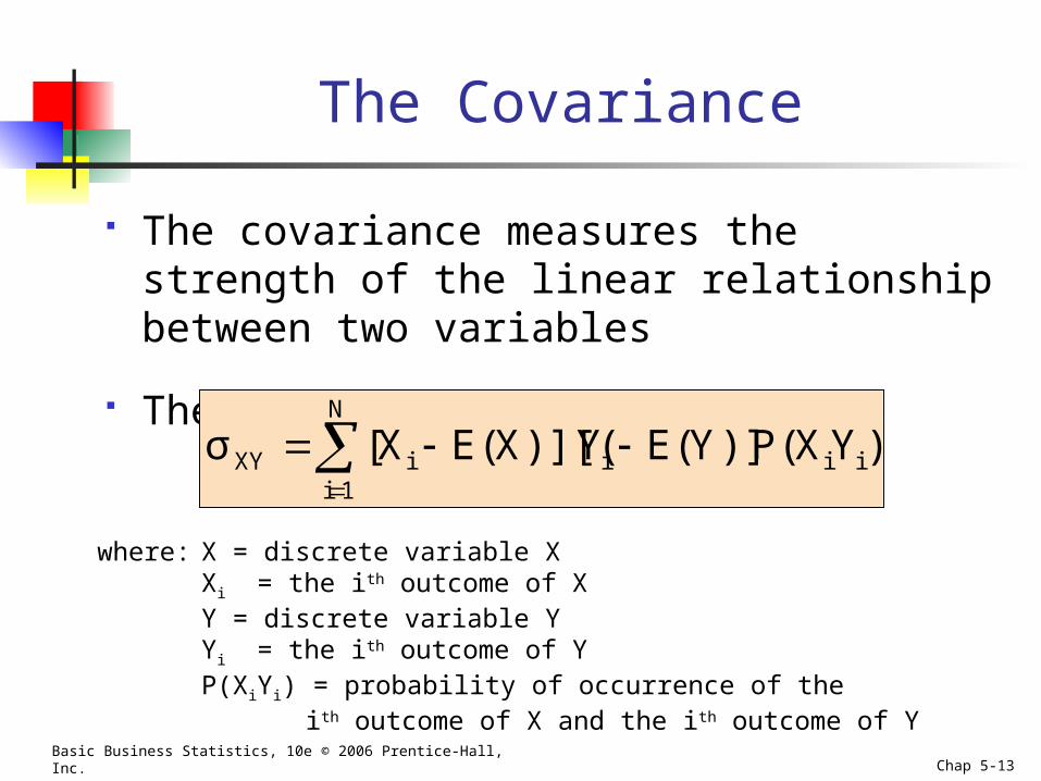
The Covariance
The covariance measures the strength of the linear relationship between two variables
The covariance:
)YX(P)]Y(EY)][(X(EX[σN
1iiiiiXY
where: X = discrete variable XXi = the ith outcome of XY = discrete variable YYi = the ith outcome of YP(XiYi) = probability of occurrence of the
ith outcome of X and the ith outcome of Y
Basic Business Statistics, 10e © 2006 Prentice-Hall, Inc. Chap 5-14
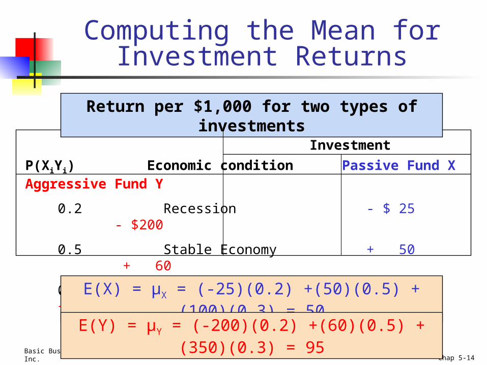
Computing the Mean for Investment Returns
Return per $1,000 for two types of investments
P(XiYi) Economic condition Passive Fund X Aggressive Fund Y
0.2 Recession - $ 25 - $200
0.5 Stable Economy + 50 + 60
0.3 Expanding Economy + 100 + 350
Investment
E(X) = μX = (-25)(0.2) +(50)(0.5) + (100)(0.3) = 50
E(Y) = μY = (-200)(0.2) +(60)(0.5) + (350)(0.3) = 95
Basic Business Statistics, 10e © 2006 Prentice-Hall, Inc. Chap 5-15
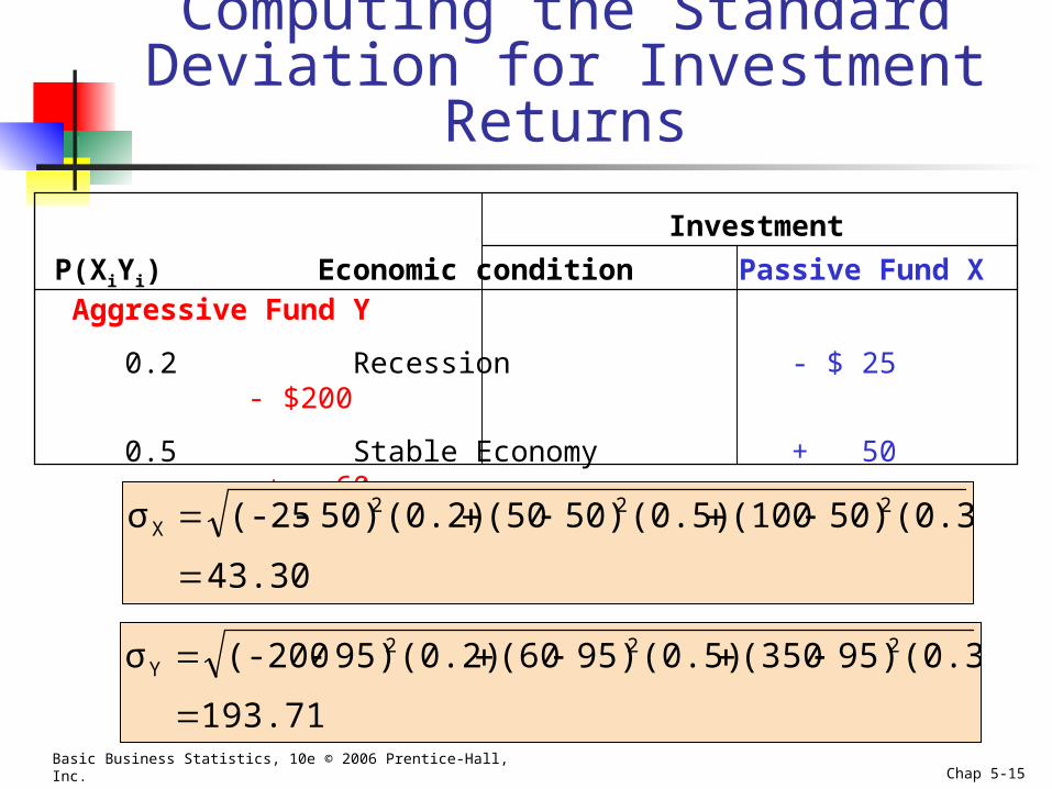
Computing the Standard Deviation for Investment Returns
P(XiYi) Economic condition Passive Fund X Aggressive Fund Y
0.2 Recession - $ 25 - $200
0.5 Stable Economy + 50 + 60
0.3 Expanding Economy + 100 + 350
Investment
43.30
(0.3)50)(100(0.5)50)(50(0.2)50)(-25σ 222X
193.71
(0.3)95)(350(0.5)95)(60(0.2)95)(-200σ 222Y
Basic Business Statistics, 10e © 2006 Prentice-Hall, Inc. Chap 5-16
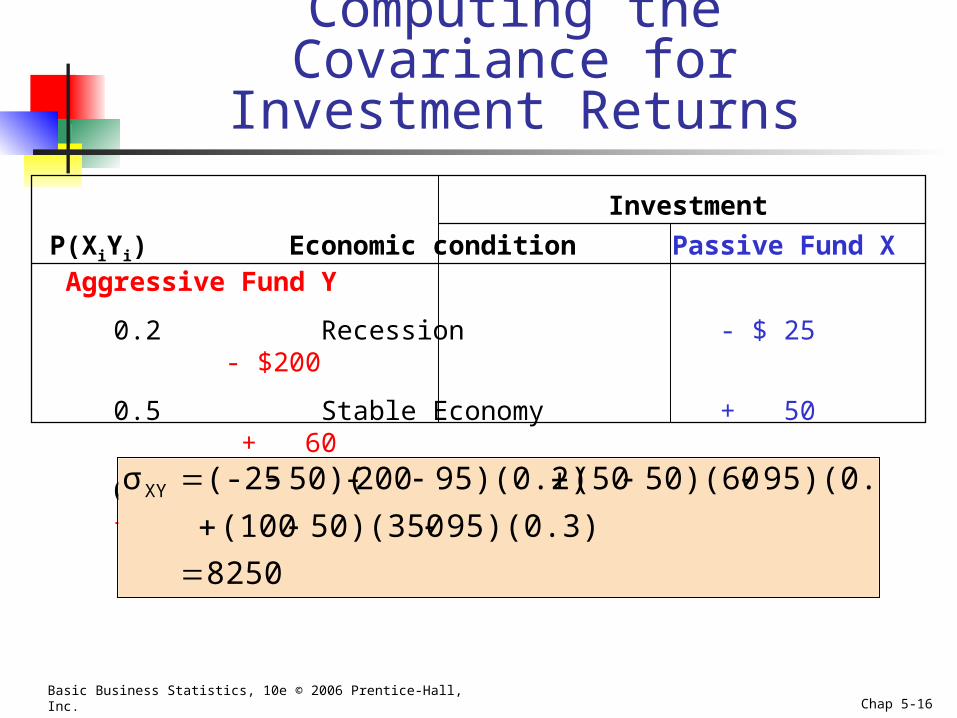
Computing the Covariance for Investment Returns
P(XiYi) Economic condition Passive Fund X Aggressive Fund Y
0.2 Recession - $ 25 - $200
0.5 Stable Economy + 50 + 60
0.3 Expanding Economy + 100 + 350
Investment
8250
95)(0.3)50)(350(100
95)(0.5)50)(60(5095)(0.2)200-50)((-25σXY
Basic Business Statistics, 10e © 2006 Prentice-Hall, Inc. Chap 5-17
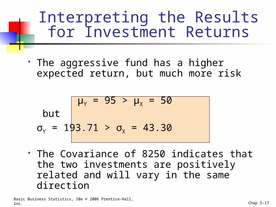
Interpreting the Results for Investment Returns
The aggressive fund has a higher expected return, but much more risk
μY = 95 > μX = 50 but
σY = 193.71 > σX = 43.30
The Covariance of 8250 indicates that the two investments are positively related and will vary in the same direction
Basic Business Statistics, 10e © 2006 Prentice-Hall, Inc. Chap 5-18
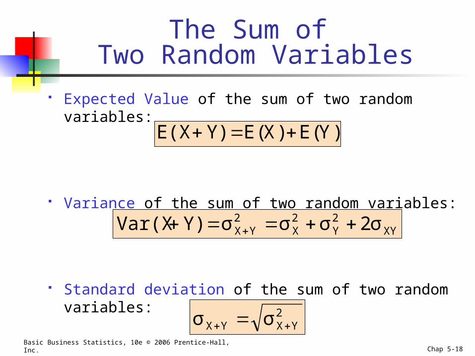
The Sum of Two Random Variables
Expected Value of the sum of two random variables:
Variance of the sum of two random variables:
Standard deviation of the sum of two random variables:
XY2Y
2X
2YX σ2σσσY)Var(X
)Y(E)X(EY)E(X
2YXYX σσ
Basic Business Statistics, 10e © 2006 Prentice-Hall, Inc. Chap 5-19
Portfolio Expected Return and Portfolio Risk
Portfolio expected return (weighted average return):
Portfolio risk (weighted variability)
Where w = portion of portfolio value in asset X
(1 - w) = portion of portfolio value in asset Y
)Y(E)w1()X(EwE(P)
XY2Y
22X
2P w)σ-2w(1σ)w1(σwσ
Basic Business Statistics, 10e © 2006 Prentice-Hall, Inc. Chap 5-20
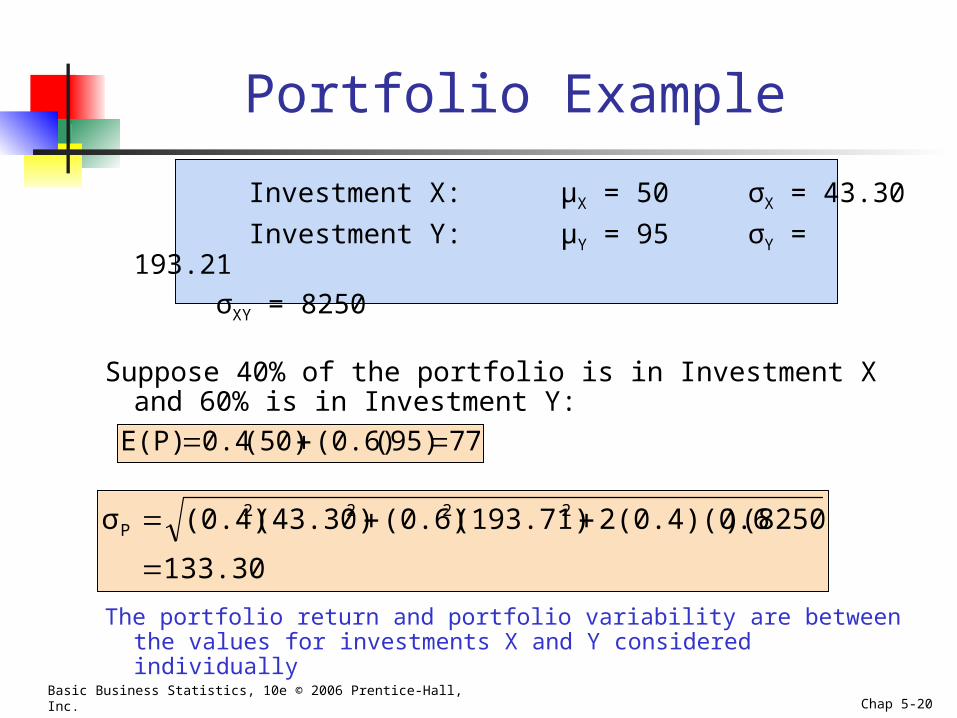
Portfolio Example
Investment X: μX = 50 σX = 43.30
Investment Y: μY = 95 σY = 193.21
σXY = 8250
Suppose 40% of the portfolio is in Investment X and 60% is in Investment Y:
The portfolio return and portfolio variability are between the values for investments X and Y considered individually
77(95)(0.6)(50)0.4E(P)
133.30
)(8250)2(0.4)(0.6(193.71)(0.6)(43.30)(0.4)σ 2222P
Basic Business Statistics, 10e © 2006 Prentice-Hall, Inc. Chap 5-21
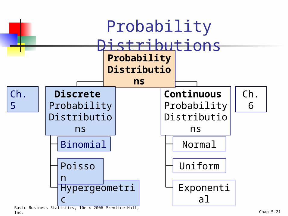
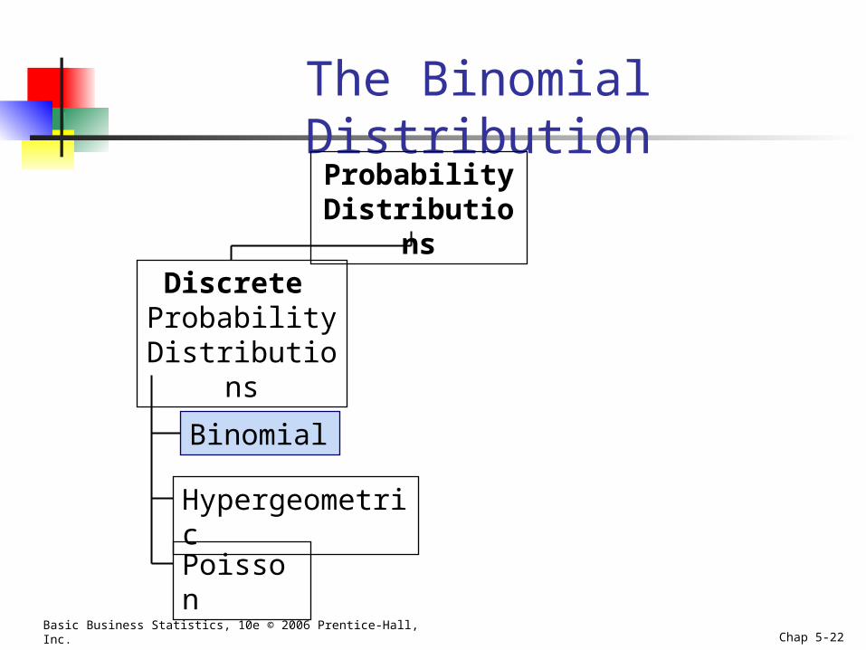
Probability Distributions
Continuous Probability
Distributions
Binomial
Hypergeometric
Poisson
Probability Distributions
Discrete Probability
Distributions
Normal
Uniform
Exponential
Ch. 5 Ch. 6
Basic Business Statistics, 10e © 2006 Prentice-Hall, Inc. Chap 5-22
The Binomial Distribution
Binomial
Hypergeometric
Poisson
Probability Distributions
Discrete Probability
Distributions
Basic Business Statistics, 10e © 2006 Prentice-Hall, Inc. Chap 5-23
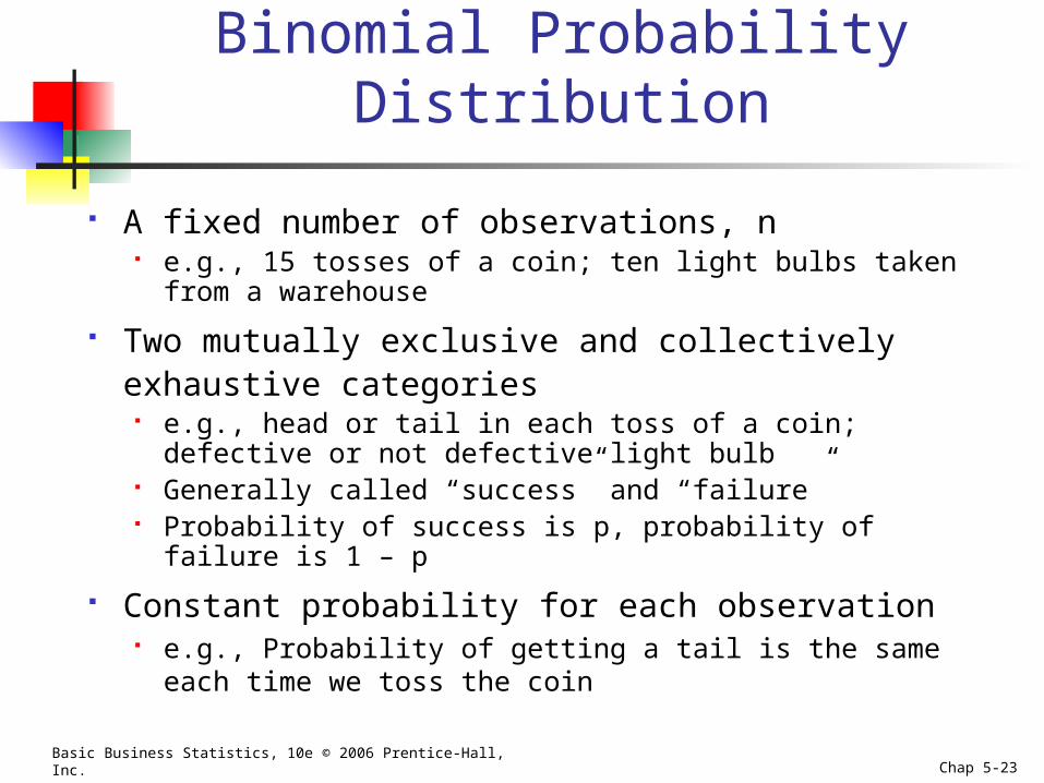
Binomial Probability Distribution
A fixed number of observations, n e.g., 15 tosses of a coin; ten light bulbs taken from a warehouse
Two mutually exclusive and collectively exhaustive categories
e.g., head or tail in each toss of a coin; defective or not defective light bulb
Generally called “success” and “failure” Probability of success is p, probability of failure is 1 – p
Constant probability for each observation e.g., Probability of getting a tail is the same each time we toss
the coin
Basic Business Statistics, 10e © 2006 Prentice-Hall, Inc. Chap 5-24
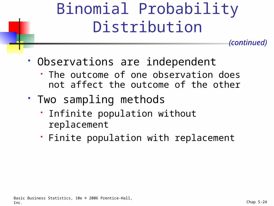
Binomial Probability Distribution(continued)
Observations are independent The outcome of one observation does not affect the
outcome of the other Two sampling methods
Infinite population without replacement Finite population with replacement
Basic Business Statistics, 10e © 2006 Prentice-Hall, Inc. Chap 5-25
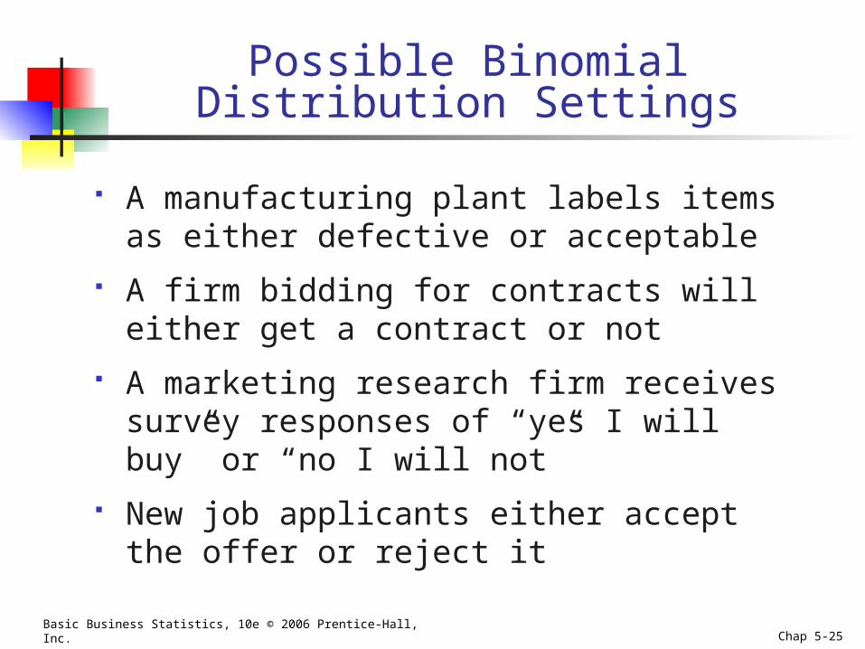
Possible Binomial Distribution Settings
A manufacturing plant labels items as either defective or acceptable
A firm bidding for contracts will either get a contract or not
A marketing research firm receives survey responses of “yes I will buy” or “no I will not”
New job applicants either accept the offer or reject it
Basic Business Statistics, 10e © 2006 Prentice-Hall, Inc. Chap 5-26
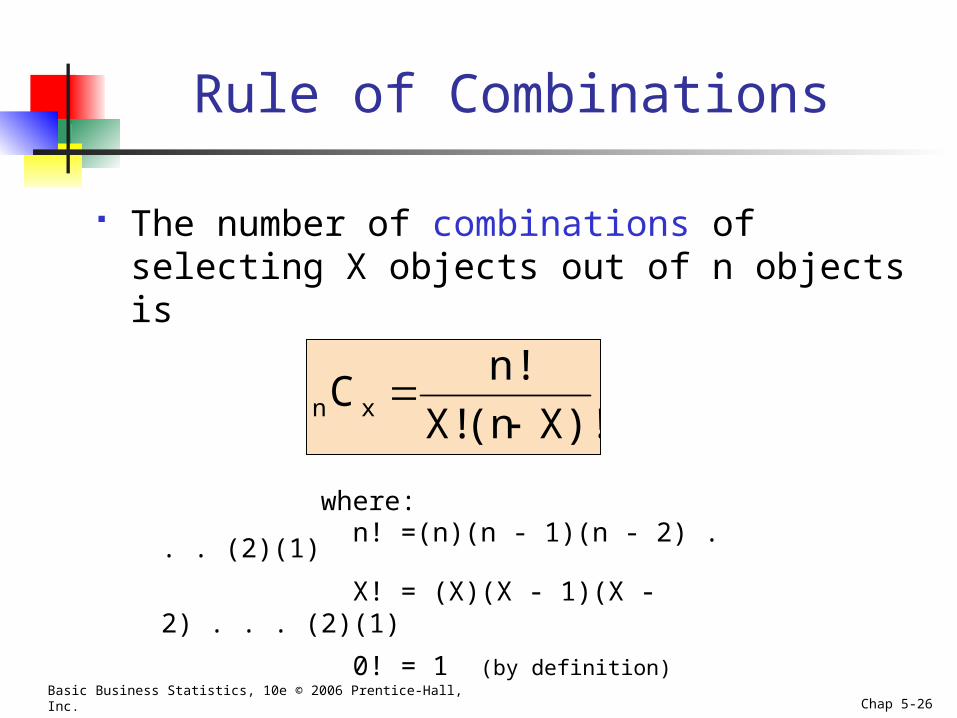
Rule of Combinations
The number of combinations of selecting X objects out of n objects is
X)!(nX!
n!Cxn
where:n! =(n)(n - 1)(n - 2) . . . (2)(1)
X! = (X)(X - 1)(X - 2) . . . (2)(1)
0! = 1 (by definition)
Basic Business Statistics, 10e © 2006 Prentice-Hall, Inc. Chap 5-27
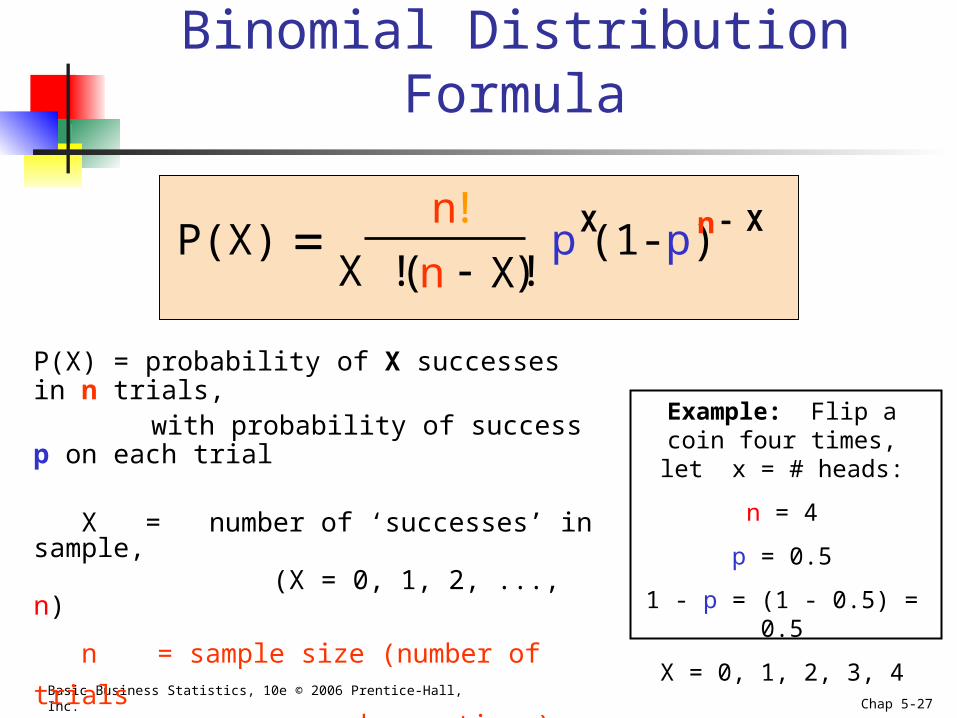
P(X) = probability of X successes in n trials, with probability of success p on each trial
X = number of ‘successes’ in sample, (X = 0, 1, 2, ..., n)
n = sample size (number of trials or observations)
p = probability of “success”
P(X)n
X ! n Xp (1-p)X n X!
( )!
Example: Flip a coin four times, let x = # heads:
n = 4
p = 0.5
1 - p = (1 - 0.5) = 0.5
X = 0, 1, 2, 3, 4
Binomial Distribution Formula
Basic Business Statistics, 10e © 2006 Prentice-Hall, Inc. Chap 5-28
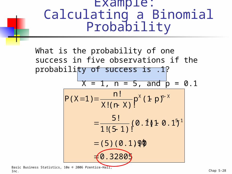
Example: Calculating a Binomial Probability
What is the probability of one success in five observations if the probability of success is .1?
X = 1, n = 5, and p = 0.1
0.32805
.9)(5)(0.1)(0
0.1)(1(0.1)1)!(51!
5!
p)(1pX)!(nX!
n!1)P(X
4
151
XnX
Basic Business Statistics, 10e © 2006 Prentice-Hall, Inc. Chap 5-29
n = 5 p = 0.1
n = 5 p = 0.5
Mean
0.2.4.6
0 1 2 3 4 5
X
P(X)
.2
.4
.6
0 1 2 3 4 5
X
P(X)
0
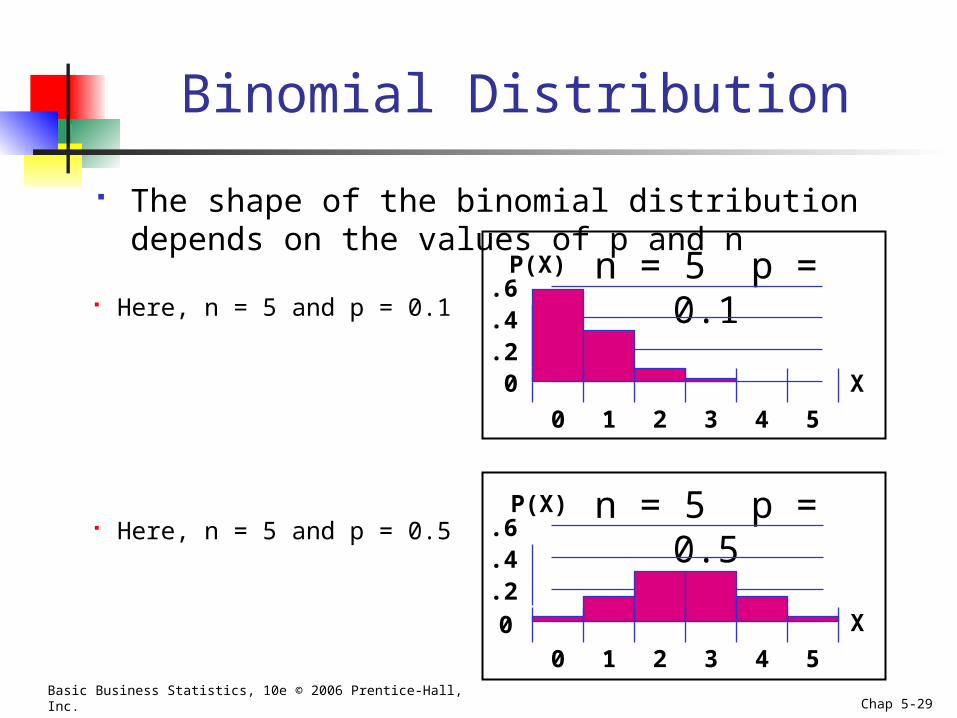
Binomial Distribution
The shape of the binomial distribution depends on the values of p and n
Here, n = 5 and p = 0.1
Here, n = 5 and p = 0.5
Basic Business Statistics, 10e © 2006 Prentice-Hall, Inc. Chap 5-30
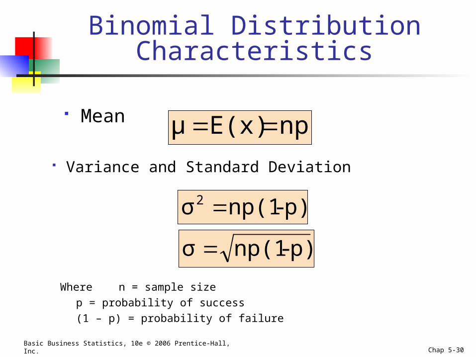
Binomial Distribution Characteristics
Mean
Variance and Standard Deviation
npE(x)μ
p)-np(1σ2
p)-np(1σ
Where n = sample size
p = probability of success
(1 – p) = probability of failure
Basic Business Statistics, 10e © 2006 Prentice-Hall, Inc. Chap 5-31
二項機率分配之期望值與變異數 設 X為一二項隨機變數,其機率函數為:
f x C p q x nxn x n x( ) , , , , 0 1 2
則其期望值為: E X np( )
變異數為: V X npq( )
證明 茲證明二項分配的期望值與變異數如下:
(1)期望值
E X xf xx
n( ) ( )
0
xC p qx
n x n x
x
n
0
x
n
n x xp qx n x
x
n !
( )! !0
1
0
1
1 !)!1(
)!1(
)!1()!(
)!1( n
y
ynyn
x
xnx qpyyn
nnpqp
xxn
nn
「式中 )1( xy 」
np p q n( ) 1
(利用 )1( n 次方的二項展開式)
np
Basic Business Statistics, 10e © 2006 Prentice-Hall, Inc. Chap 5-32
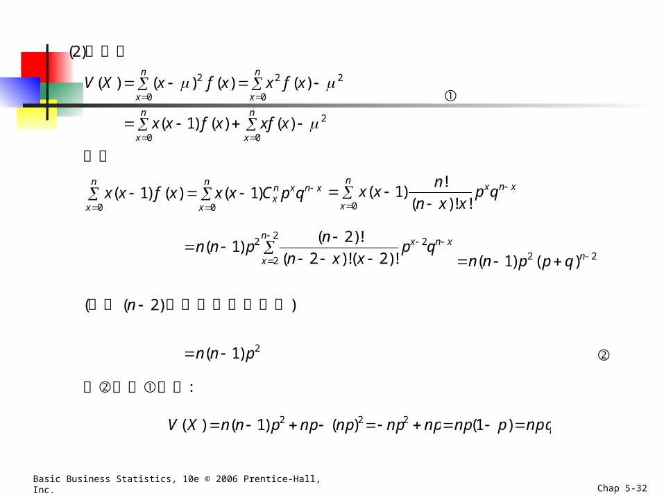
(2)變異數
2
00
2
0
2
0
2
)()()1(
)()()()(
n
x
n
x
n
x
n
x
xxfxfxx
xfxxfxXV
其中
x x f x x x C p qxn x n x
x
n
x
n( ) ( ) ( )
1 1
00
x x
n
n x xp qx n x
x
n( )
!
( )! !1
0
n n p
n
n x xp qx n x
x
n( )
( )!
( )!( )!1
2
2 22 2
2
2
n n p p q n( ) ( )1 2 2
(利用 )2( n 次方的二次展開式)
n n p( )1 2
將代入可得:
V X n n p np np( ) ( ) ( ) 1 2 2 np np2 np p( )1 npq

Basic Business Statistics, 10e © 2006 Prentice-Hall, Inc. Chap 5-33

Basic Business Statistics, 10e © 2006 Prentice-Hall, Inc. Chap 5-34
Basic Business Statistics, 10e © 2006 Prentice-Hall, Inc. Chap 5-35
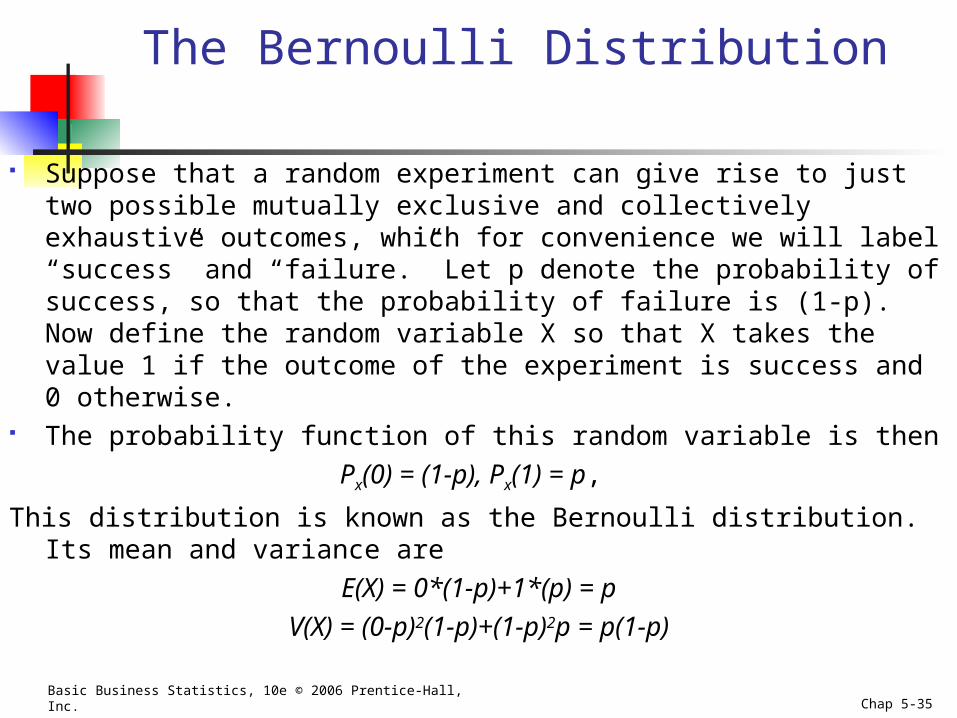
The Bernoulli Distribution
Suppose that a random experiment can give rise to just two possible mutually exclusive and collectively exhaustive outcomes, which for convenience we will label “success” and “failure.” Let p denote the probability of success, so that the probability of failure is (1-p). Now define the random variable X so that X takes the value 1 if the outcome of the experiment is success and 0 otherwise.
The probability function of this random variable is then
Px(0) = (1-p), Px(1) = p,
This distribution is known as the Bernoulli distribution. Its mean and variance are
E(X) = 0*(1-p)+1*(p) = p
V(X) = (0-p)2(1-p)+(1-p)2p = p(1-p)
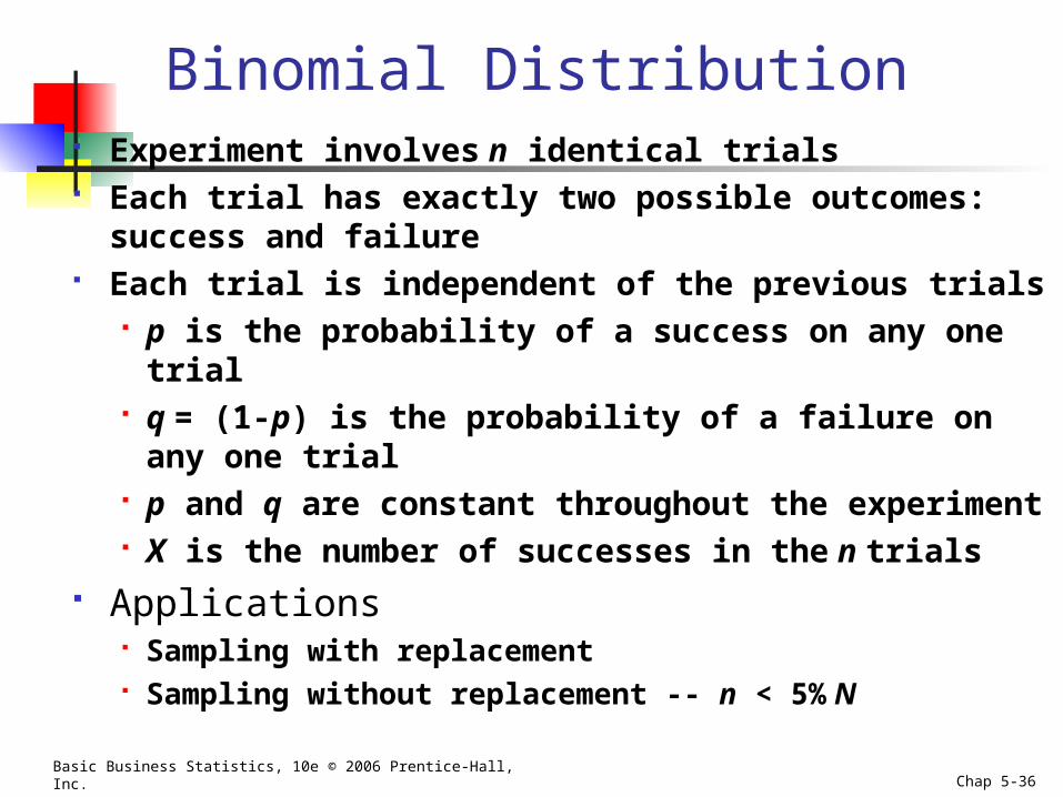
Basic Business Statistics, 10e © 2006 Prentice-Hall, Inc. Chap 5-36
Binomial Distribution Experiment involves n identical trials Each trial has exactly two possible outcomes: success
and failure Each trial is independent of the previous trials
p is the probability of a success on any one trial q = (1-p) is the probability of a failure on any one trial p and q are constant throughout the experiment X is the number of successes in the n trials
Applications Sampling with replacement Sampling without replacement -- n < 5% N
Basic Business Statistics, 10e © 2006 Prentice-Hall, Inc. Chap 5-37
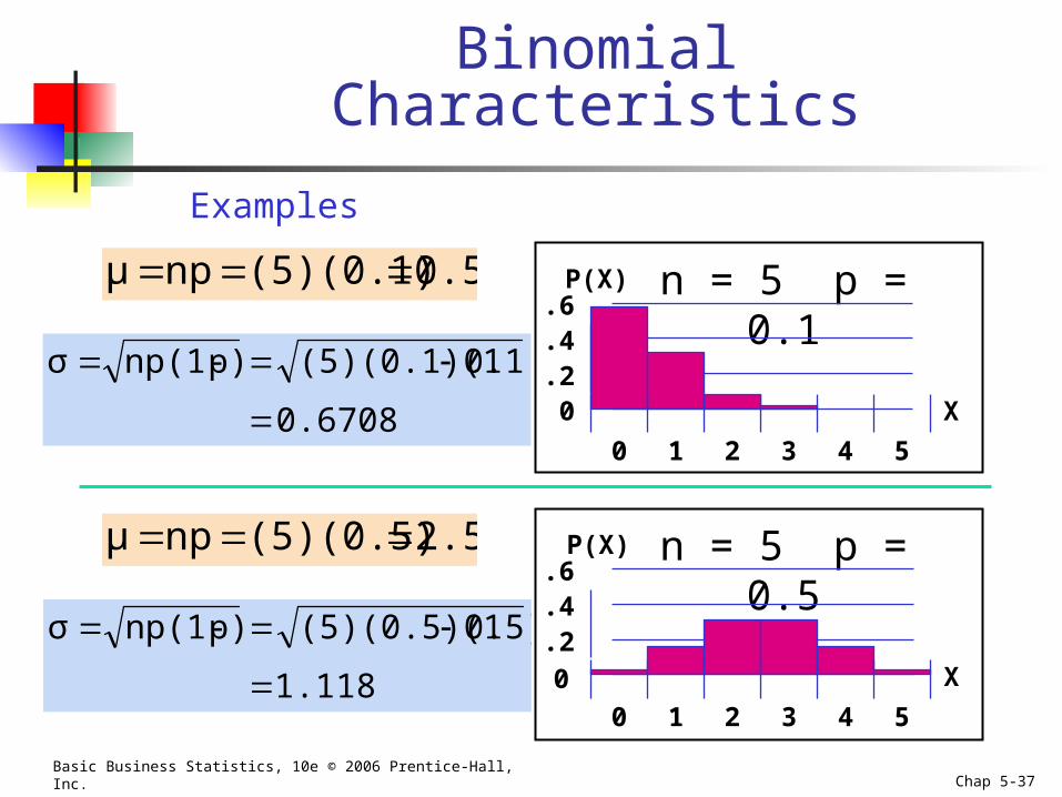
n = 5 p = 0.1
n = 5 p = 0.5
Mean
0.2.4.6
0 1 2 3 4 5
X
P(X)
.2
.4
.6
0 1 2 3 4 5
X
P(X)
0
0.5(5)(0.1)npμ
0.6708
0.1)(5)(0.1)(1p)np(1-σ
2.5(5)(0.5)npμ
1.118
0.5)(5)(0.5)(1p)np(1-σ
Binomial Characteristics
Examples
Basic Business Statistics, 10e © 2006 Prentice-Hall, Inc. Chap 5-38
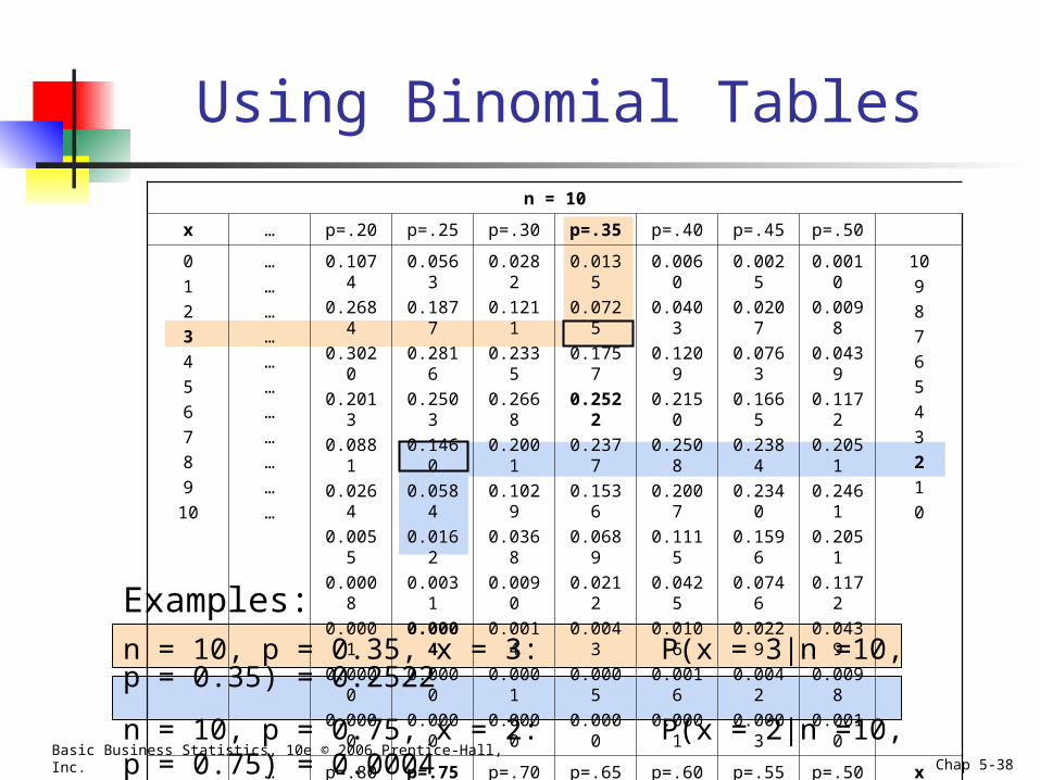
Using Binomial Tables
n = 10
x … p=.20 p=.25 p=.30 p=.35 p=.40 p=.45 p=.50
0
1
2
3
4
5
6
7
8
9
10
…
…
…
…
…
…
…
…
…
…
…
0.1074
0.2684
0.3020
0.2013
0.0881
0.0264
0.0055
0.0008
0.0001
0.0000
0.0000
0.0563
0.1877
0.2816
0.2503
0.1460
0.0584
0.0162
0.0031
0.0004
0.0000
0.0000
0.0282
0.1211
0.2335
0.2668
0.2001
0.1029
0.0368
0.0090
0.0014
0.0001
0.0000
0.0135
0.0725
0.1757
0.2522
0.2377
0.1536
0.0689
0.0212
0.0043
0.0005
0.0000
0.0060
0.0403
0.1209
0.2150
0.2508
0.2007
0.1115
0.0425
0.0106
0.0016
0.0001
0.0025
0.0207
0.0763
0.1665
0.2384
0.2340
0.1596
0.0746
0.0229
0.0042
0.0003
0.0010
0.0098
0.0439
0.1172
0.2051
0.2461
0.2051
0.1172
0.0439
0.0098
0.0010
10
9
8
7
6
5
4
3
2
1
0
… p=.80 p=.75 p=.70 p=.65 p=.60 p=.55 p=.50 x
Examples: n = 10, p = 0.35, x = 3: P(x = 3|n =10, p = 0.35) = 0.2522
n = 10, p = 0.75, x = 2: P(x = 2|n =10, p = 0.75) = 0.0004
Basic Business Statistics, 10e © 2006 Prentice-Hall, Inc. Chap 5-39
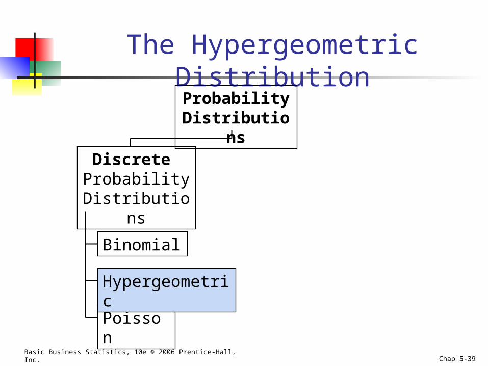
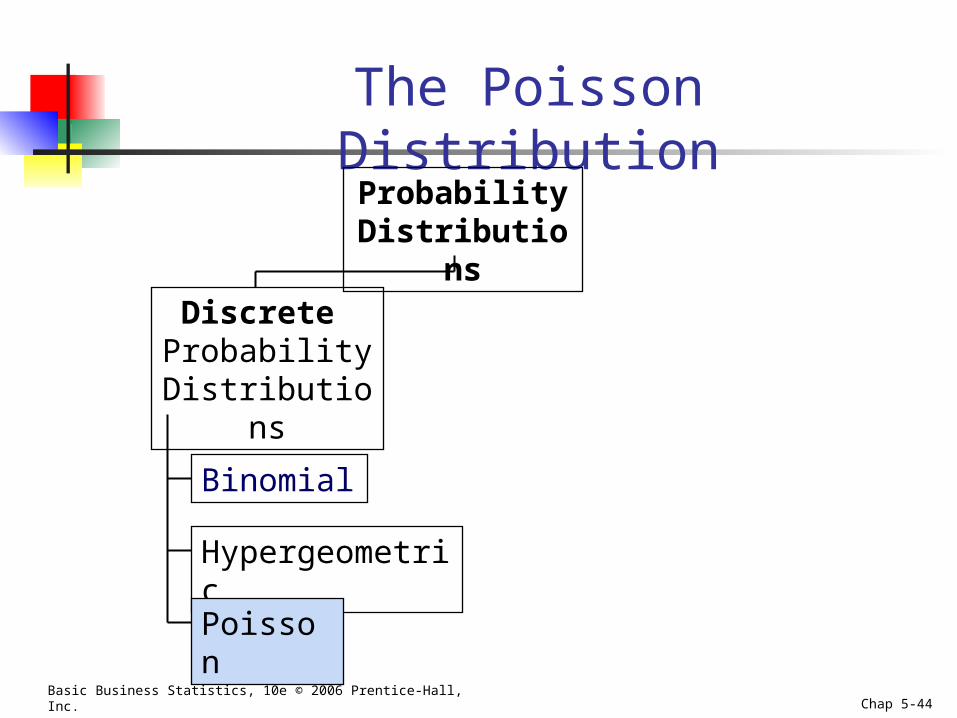
The Hypergeometric Distribution
Binomial
Poisson
Probability Distributions
Discrete Probability
Distributions
Hypergeometric
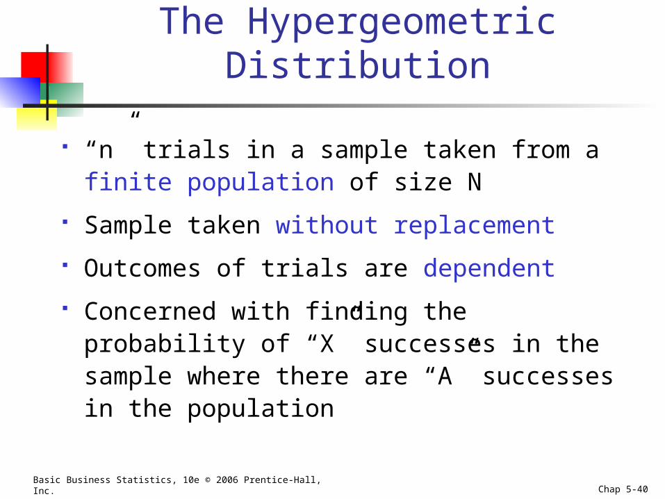
Basic Business Statistics, 10e © 2006 Prentice-Hall, Inc. Chap 5-40
The Hypergeometric Distribution
“n” trials in a sample taken from a finite population of size N
Sample taken without replacement
Outcomes of trials are dependent
Concerned with finding the probability of “X” successes in the sample where there are “A” successes in the population
Basic Business Statistics, 10e © 2006 Prentice-Hall, Inc. Chap 5-41
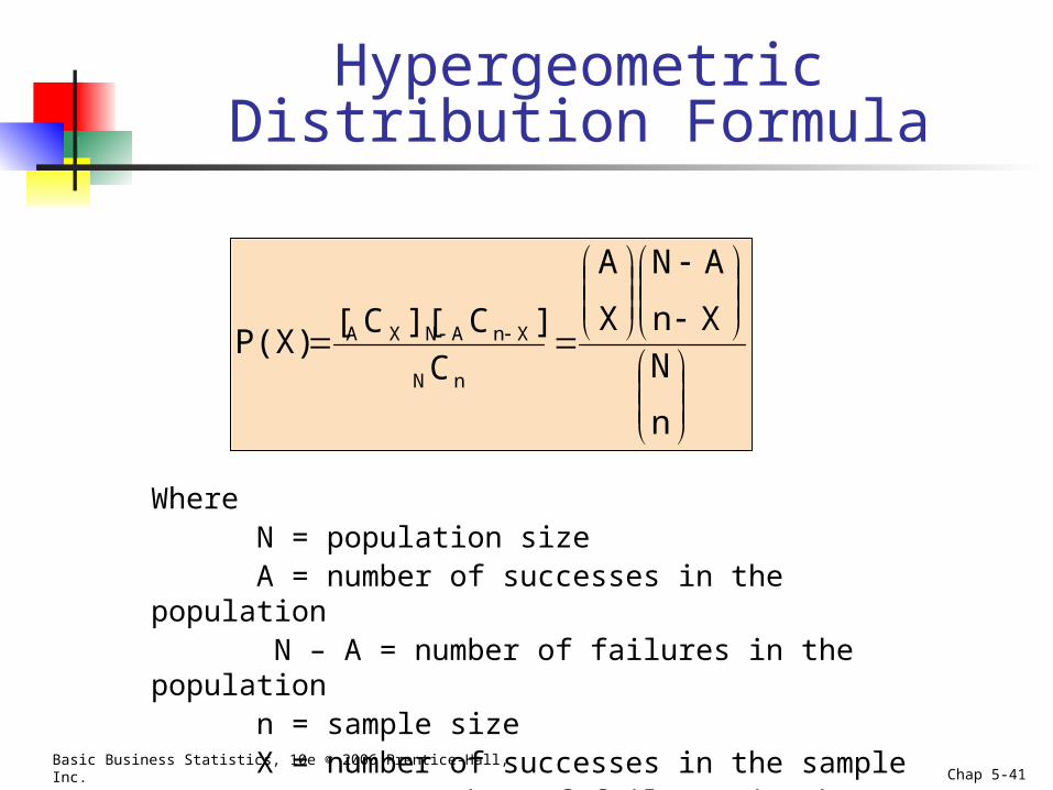
Hypergeometric Distribution Formula
n
N
Xn
AN
X
A
C
]C][C[P(X)
nN
XnANXA
WhereN = population sizeA = number of successes in the population
N – A = number of failures in the populationn = sample sizeX = number of successes in the sample
n – X = number of failures in the sample
Basic Business Statistics, 10e © 2006 Prentice-Hall, Inc. Chap 5-42
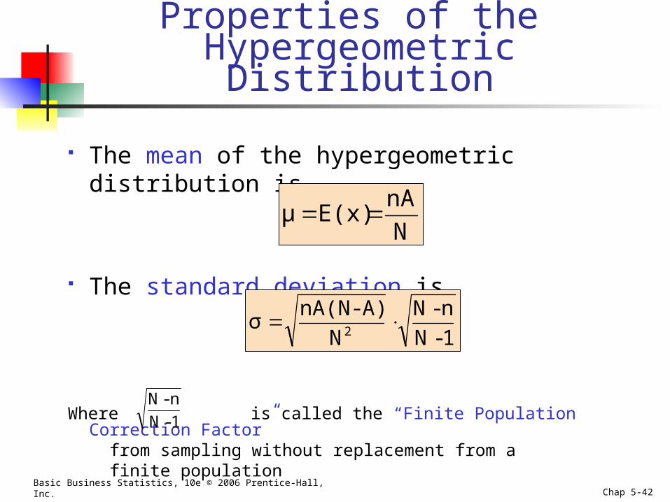
Properties of the Hypergeometric Distribution
The mean of the hypergeometric distribution is
The standard deviation is
Where is called the “Finite Population Correction Factor” from sampling without replacement from a finite population
N
nAE(x)μ
1- N
n-N
N
A)-nA(Nσ
2
1- N
n-N

Basic Business Statistics, 10e © 2006 Prentice-Hall, Inc. Chap 5-43
Using the Hypergeometric Distribution
■ Example: 3 different computers are checked from 10 in the department. 4 of the 10 computers have illegal software loaded. What is the probability that 2 of the 3 selected computers have illegal software loaded?
N = 10 n = 3 A = 4 X = 2
0.3120
(6)(6)
3
10
1
6
2
4
n
N
Xn
AN
X
A
2)P(X
The probability that 2 of the 3 selected computers have illegal software loaded is 0.30, or 30%.
Basic Business Statistics, 10e © 2006 Prentice-Hall, Inc. Chap 5-44
The Poisson Distribution
Binomial
Hypergeometric
Poisson
Probability Distributions
Discrete Probability
Distributions
Basic Business Statistics, 10e © 2006 Prentice-Hall, Inc. Chap 5-45
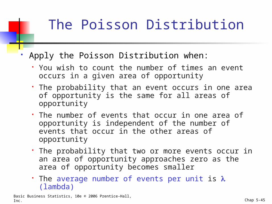
The Poisson Distribution
Apply the Poisson Distribution when: You wish to count the number of times an event
occurs in a given area of opportunity The probability that an event occurs in one area of
opportunity is the same for all areas of opportunity The number of events that occur in one area of
opportunity is independent of the number of events that occur in the other areas of opportunity
The probability that two or more events occur in an area of opportunity approaches zero as the area of opportunity becomes smaller
The average number of events per unit is (lambda)
Basic Business Statistics, 10e © 2006 Prentice-Hall, Inc. Chap 5-46
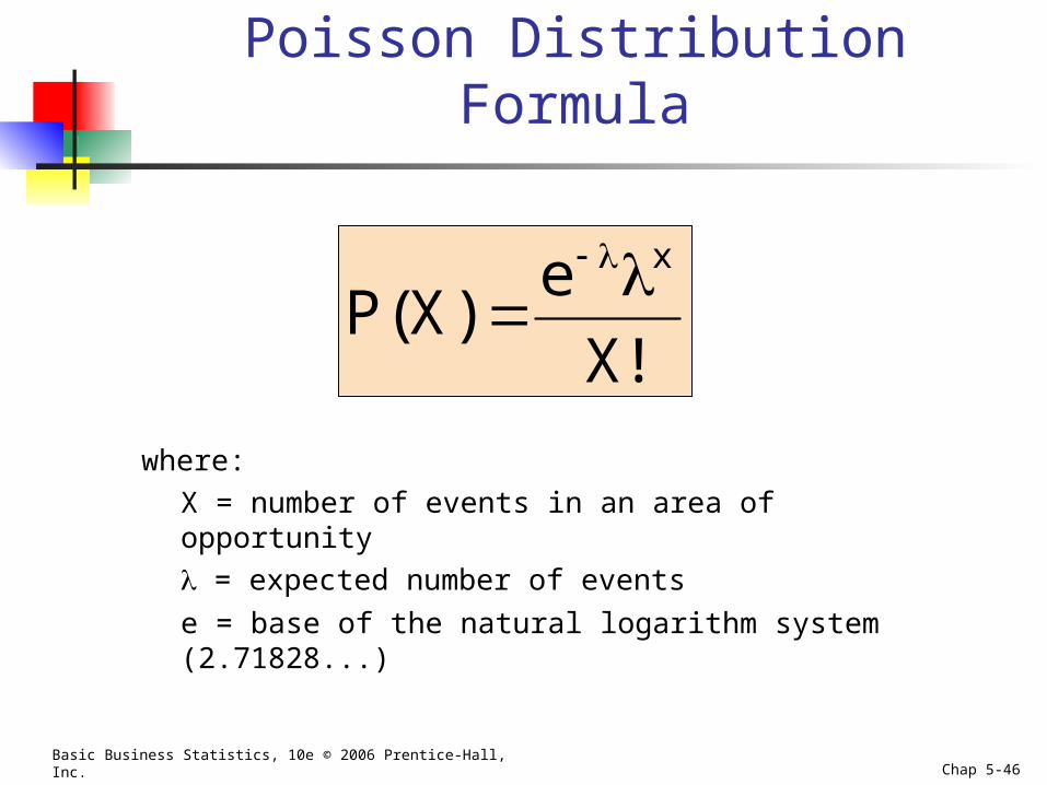
Poisson Distribution Formula
where:
X = number of events in an area of opportunity
= expected number of events
e = base of the natural logarithm system (2.71828...)
!X
e)X(P
x
Basic Business Statistics, 10e © 2006 Prentice-Hall, Inc. Chap 5-47
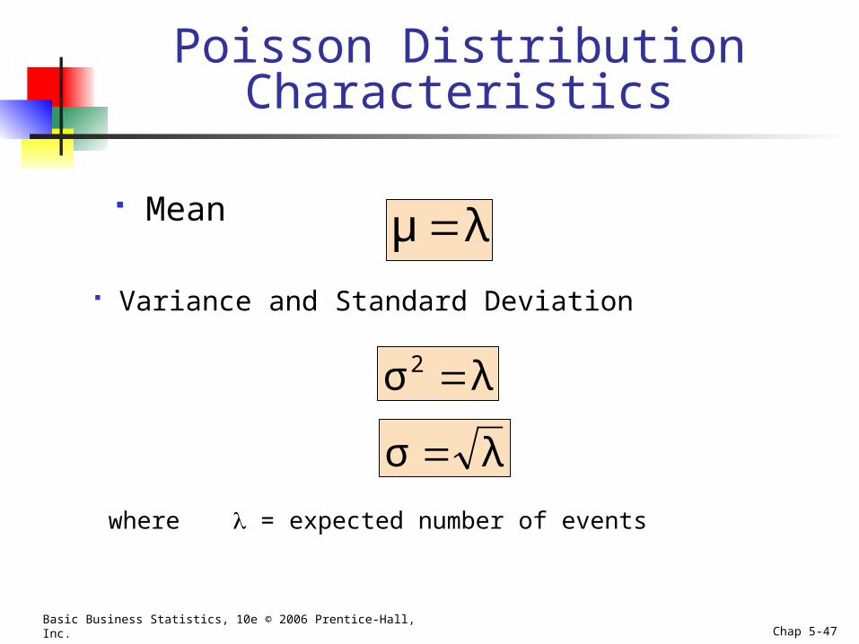
Poisson Distribution Characteristics
Mean
Variance and Standard Deviation
λμ
λσ2
λσ
where = expected number of events
Basic Business Statistics, 10e © 2006 Prentice-Hall, Inc. Chap 5-48
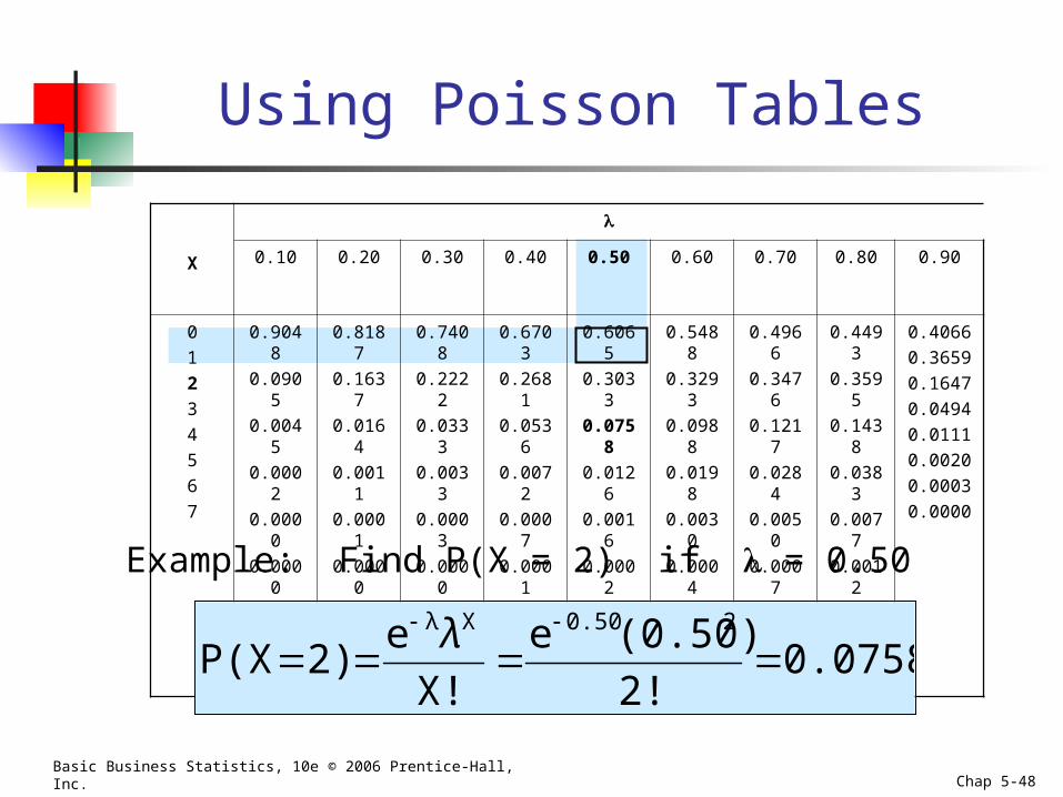
Using Poisson Tables
X
0.10 0.20 0.30 0.40 0.50 0.60 0.70 0.80 0.90
0
1
2
3
4
5
6
7
0.9048
0.0905
0.0045
0.0002
0.0000
0.0000
0.0000
0.0000
0.8187
0.1637
0.0164
0.0011
0.0001
0.0000
0.0000
0.0000
0.7408
0.2222
0.0333
0.0033
0.0003
0.0000
0.0000
0.0000
0.6703
0.2681
0.0536
0.0072
0.0007
0.0001
0.0000
0.0000
0.6065
0.3033
0.0758
0.0126
0.0016
0.0002
0.0000
0.0000
0.5488
0.3293
0.0988
0.0198
0.0030
0.0004
0.0000
0.0000
0.4966
0.3476
0.1217
0.0284
0.0050
0.0007
0.0001
0.0000
0.4493
0.3595
0.1438
0.0383
0.0077
0.0012
0.0002
0.0000
0.4066
0.3659
0.1647
0.0494
0.0111
0.0020
0.0003
0.0000
Example: Find P(X = 2) if = 0.50
0.07582!
(0.50)e
X!
e2)P(X
20.50Xλ
λ
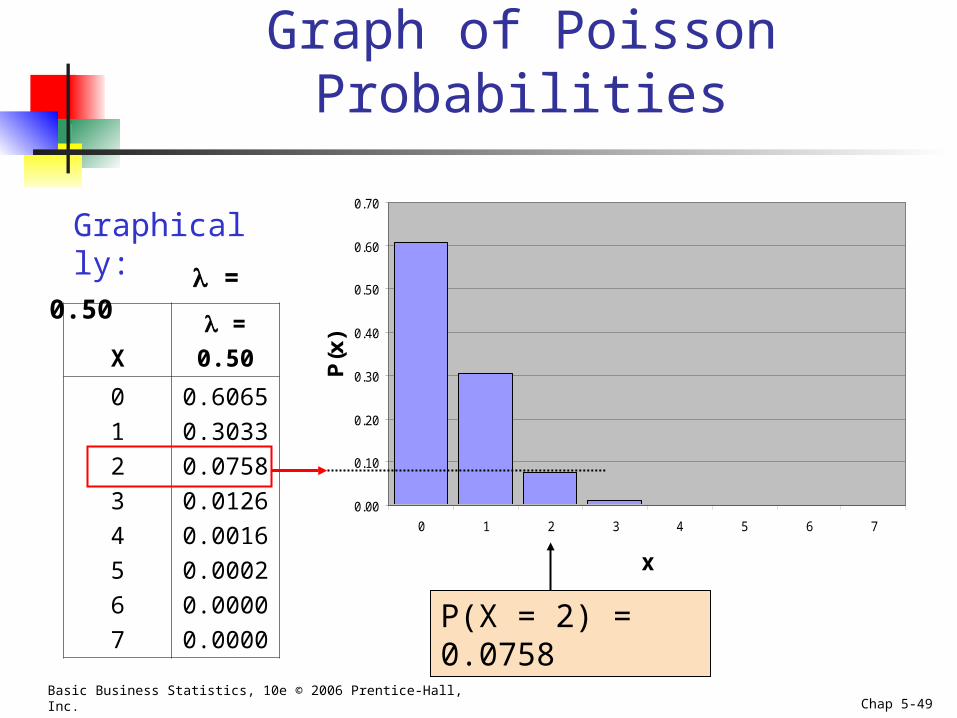
Basic Business Statistics, 10e © 2006 Prentice-Hall, Inc. Chap 5-49
Graph of Poisson Probabilities
0.00
0.10
0.20
0.30
0.40
0.50
0.60
0.70
0 1 2 3 4 5 6 7
x
P(x
)X
=
0.50
0
1
2
3
4
5
6
7
0.6065
0.3033
0.0758
0.0126
0.0016
0.0002
0.0000
0.0000P(X = 2) = 0.0758
Graphically:
= 0.50
Basic Business Statistics, 10e © 2006 Prentice-Hall, Inc. Chap 5-50
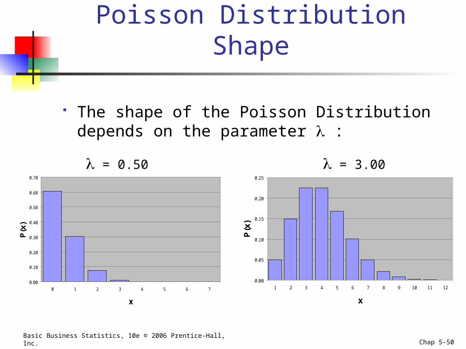
Poisson Distribution Shape
The shape of the Poisson Distribution depends on the parameter :
0.00
0.05
0.10
0.15
0.20
0.25
1 2 3 4 5 6 7 8 9 10 11 12
x
P(x
)
0.00
0.10
0.20
0.30
0.40
0.50
0.60
0.70
0 1 2 3 4 5 6 7
x
P(x
)
= 0.50 = 3.00

Basic Business Statistics, 10e © 2006 Prentice-Hall, Inc. Chap 5-51
Basic Business Statistics, 10e © 2006 Prentice-Hall, Inc. Chap 5-52
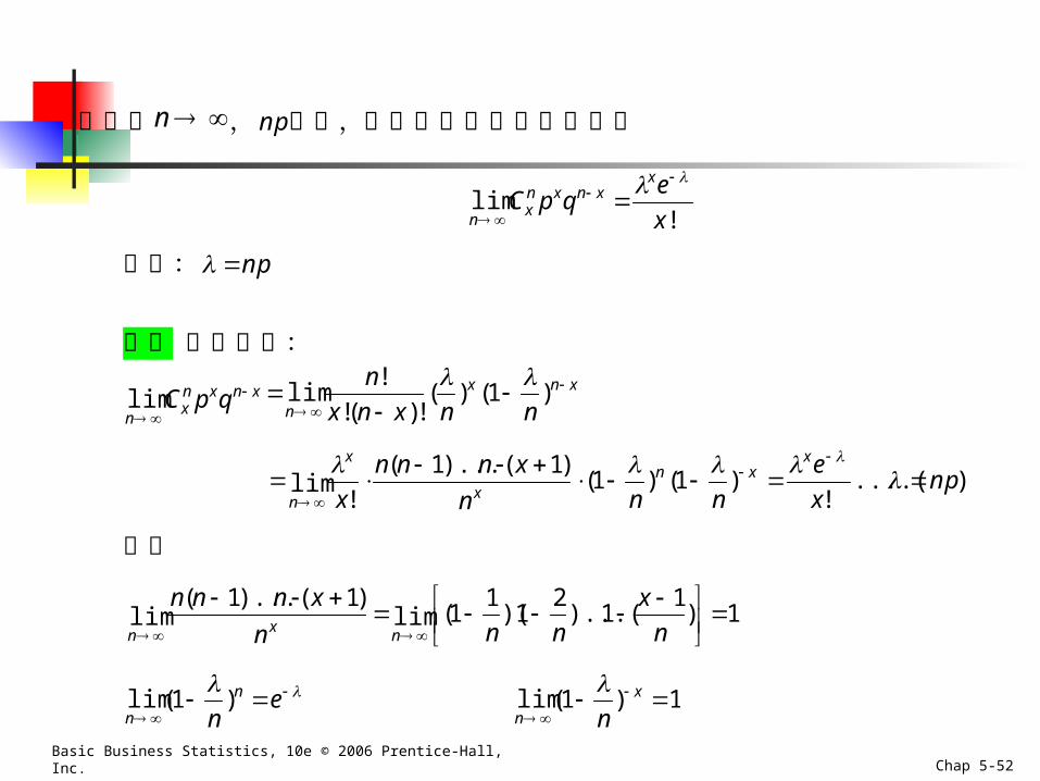
證明當n , np固定,二項分配趨近於泊松分配
lim!n
xn x n x
x
C p qe
x
式中: np
證明 證明如下:
limn
xn x n xC p q
lim!
!( )!( ) ( )
n
x n xn
x n x n n
1
)....(!
)1()1()1)...(1(
!lim np
x
e
nnn
xnnn
x
xxn
x
x
n
因為
1)1
1)...(2
1)(1
1(lim)1)...(1(
lim
n
x
nnn
xnnn
nx
n
lim( )n
n
ne
1
lim( )n
x
n
1 1
Basic Business Statistics, 10e © 2006 Prentice-Hall, Inc. Chap 5-53
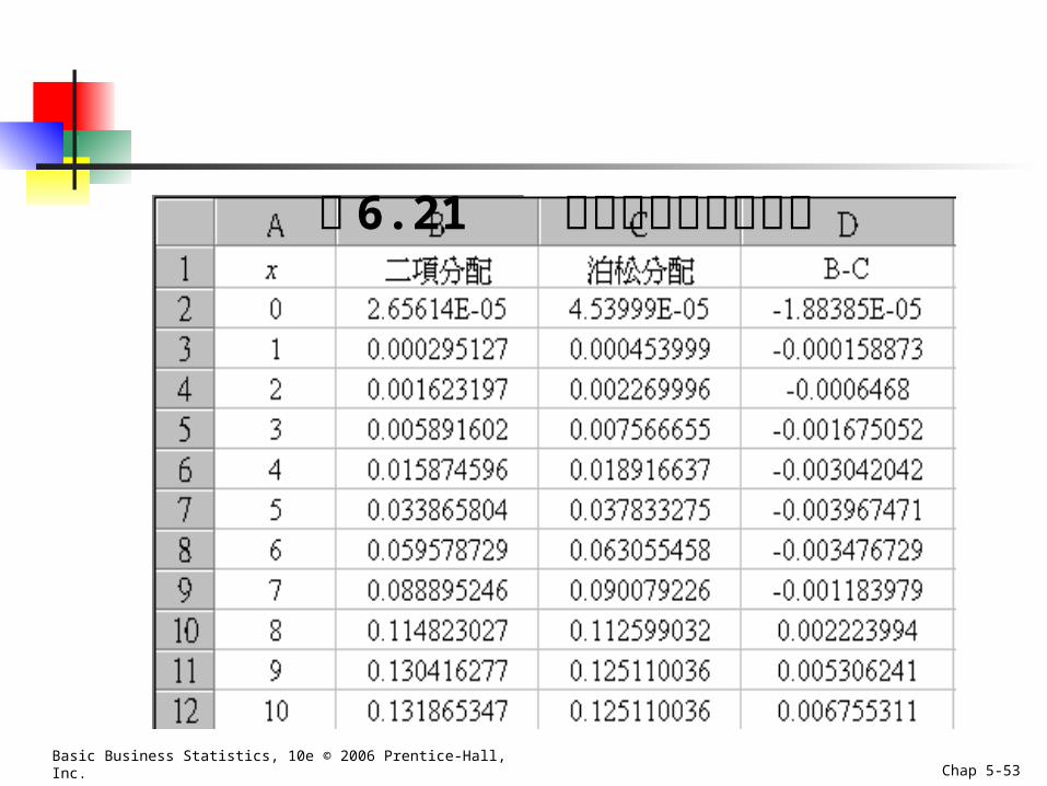
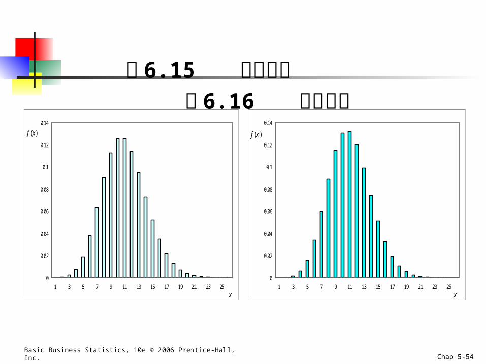
表 6.21 二項分配與泊松分配
Basic Business Statistics, 10e © 2006 Prentice-Hall, Inc. Chap 5-54
0
0.02
0.04
0.06
0.08
0.1
0.12
0.14
1 3 5 7 9 11 13 15 17 19 21 23 25
x
)(xf
0
0.02
0.04
0.06
0.08
0.1
0.12
0.14
1 3 5 7 9 11 13 15 17 19 21 23 25
x
)(xf
圖 6.15 二項分配 圖6.16 泊松分配
Basic Business Statistics, 10e © 2006 Prentice-Hall, Inc. Chap 5-55
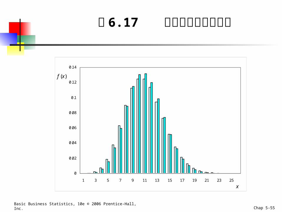
圖 6.17 二項分配與泊松分配
0
0.02
0.04
0.06
0.08
0.1
0.12
0.14
1 3 5 7 9 11 13 15 17 19 21 23 25
x
)(xf
Basic Business Statistics, 10e © 2006 Prentice-Hall, Inc. Chap 5-56
Chapter Summary
Addressed the probability of a discrete random variable
Defined covariance and discussed its application in finance
Discussed the Binomial distribution Discussed the Hypergeometric distribution Discussed the Poisson distribution