Transworld Research Network 37/661 (2), Fort P.O., Trivandrum-695 023, Kerala, India

Advanced Materials and Methods for Lithium-Ion Batteries, 2007: ISBN: 978-81-7895-279-6, Editor: Sheng Shui Zhang

20 Battery management system algorithms for HEV battery state-of-charge and state-of-health estimation

Gregory L. Plett Department of Electrical and Computer Engineering, University of Colorado at Colorado Springs, 1420 Austin Bluffs Parkway, P.O. Box 7150, Colorado Springs, CO 80933–7150, USA

Abstract The battery management system (BMS) of a

hybrid-electric-vehicle (HEV) battery pack comprises hardware and software to monitor pack status and optimize performance. One of its important functions is to execute algorithms that continuously estimate battery state-of-charge (SOC), state-of-health (SOH), and available power. The accuracy of these algorithms is critical for the proper sizing of the battery pack.

Correspondence/Reprint request: Dr. Gregory L. Plett, Department of Electrical and Computer Engineering University of Colorado at Colorado Springs, 1420 Austin Bluffs Parkway, P.O. Box 7150, Colorado Spring CO 80933–7150, USA. E-mail: glp@eas.uccs.edu

Gregory L. Plett 2

If accurate algorithms are not available, the pack—already among the costliest and heaviest components of the propulsion system—must be over-designed to compensate. This article presents methods based on Kalman filtering theory to very accurately estimate the desired quantities. While the algorithms are mathematically advanced, they can be implemented on simple and inexpensive microprocessors. The result is an important element of an economical, robust, and reliable HEV energy storage system. 1. Introduction This article presents advanced algorithms for a battery management system (BMS) for hybrid-electric vehicle (HEV) application. We assume that the BMS must be able to estimate battery state-of-charge (SOC), instantaneous available power, and parameters indicative of the battery state-of-health (SOH) such as power fade and capacity fade, and be able to adapt to changing cell characteristics over time as the cells in the battery pack age. The algorithms to be described accomplish these goals and have been successfully implemented on a Lithium-Ion Polymer Battery (LiPB) pack. A hybrid-electric vehicle is one with both a gasoline (or diesel) engine and an electric motor. In the most common configuration commercially available, both the engine and the motor are coupled directly to the power train, where the motor provides boost energy to supplement the engine and acts as a generator when coasting, braking, or when the engine can supply extra power to charge the battery pack. Such “parallel-hybrid” systems are cost effective as their battery packs can be modestly sized. Even so, and because of the demanding requirements on a pack of limited capacity, advanced methods must be used to estimate SOC, SOH, and instantaneous power in order to safely, efficiently and aggressively exploit the pack capabilities. The battery pack of an HEV comprises a number of sub-components: the cells themselves (typically wired in series to generate a high voltage, but sometimes also wired in parallel to develop higher currents), power electronics to disconnect the pack should there exist an unsafe operating condition, a thermal conditioning system, the electronic BMS, and sensors for voltages, current, and temperature. The BMS is frequently microprocessor based, which allows flexibility in the kinds of algorithms that can be executed. Various algorithms for SOC estimation (in particular) have been very well explained elsewhere in a few excellent tutorial articles [1,2]. Instead of duplicating these efforts, we focus here on the approach that has been the most successful in our own experience: variants of the ubiquitous Kalman filter, which is an algorithm for estimating the present value of the time-varying unmeasurable “state” of a dynamic system. Kalman filters were introduced in 1960 [3,4] in the context of estimating hidden system states for the purpose of

BMS algorithms for HEV SOC and SOH estimation 3

controlling a linear system, for which they are the optimal solution, and are now commonly employed in control systems, communications, defense, image processing, space, and GPS navigation applications. A unique benefit of the Kalman filter over other estimation approaches is that it automatically provides dynamic error-bounds on its own state estimates. By modeling our battery system to include the wanted unknown quantities in its state description, a Kalman filter estimates their values and gives error bounds on the estimates. We exploit this fact to give aggressive performance from our battery pack, without fear of causing damage by over-charge or over-discharge. At first glance, the equations and theory behind Kalman filtering can appear opaque. It is obvious to ask whether the HEV BMS application requires such complexity. The answer to this question depends on the design specifications given to the BMS software engineers for the errors allowed on estimates of SOC, SOH, and maximum power. These specifications are often very aggressive since being able to optimize the cost, weight, size and reliability of major HEV systems is critical to maximizing the value of the HEV to the end customer1. In order to counteract imprecise algorithms, one has to over-design the rest of the pack—a one-time expense of algorithm development can quickly overcome the accumulated per-unit cost of an over designed battery pack. To that end, advanced algorithms are often warranted, and we do not know of any algorithms able to produce better estimates than those presented here. Further, the simple algorithms typical of a portable-electronic battery pack just don’t work in the HEV environment. One reason is that the cells in an HEV battery pack are very rarely in an equilibrium state (ruling out simple voltage measurements to predict SOC via the cell’s OCV versus SOC relationship). This is due to HEVs requiring very high electrical current relative to the capacity of the cells, with present vehicles demanding up to ±20 times the C-rate, and future systems presently in development requiring higher relative rates2. The rate profile (current as a function of time) for HEV is also very dynamic as HEVs are typically designed so that the battery/motor system handles the instantaneous load transients and the engine handles the average load [5,6]. Coulomb-counting methods also cannot be used as they inherently integrate any error of the current sensor, and become unstable without some __________________________ 1Of the components comprising the propulsion of an HEV, the costliest is the battery pack, which may represent 30−35% of the total cost of the propulsion system. The battery is among the heaviest components of the propulsion system as well. Therefore, careful design of the battery pack and the BMS can dramatically impact the lifetime affordability of an HEV. 2The “C-rate” of a cell refers to the nominal capacity of the cell divided by one hour, and thus is the constant-current rate required to discharge a cell in one hour from a fully charged a priori condition. It is measured in amperes or milli-amperes.

Gregory L. Plett 4

reset mechanism. HEV battery packs are never fully recharged to a known SOC, so simple reset mechanisms are not available. Ad hoc combinations of these two approaches are often attempted, employing reset mechanisms and correction factors for age, temperature, and so forth, but we feel that the resulting complexity ends up to be greater than that of the Kalman filter. In summary, we propose that the kinds of algorithms presented in this article provide the best solution for robust long-term deployment. We now proceed by discussing requirements for a BMS in the HEV environment. We then introduce the concept of model-based state estimation, present the sigma-point Kalman filter (SPKF) as an example, and proceed to show how model parameters can also be estimated using a “joint SPKF.” Using the output of the joint SPKF, we show how to predict pack power and calculate cells to be equalized. We present some simulation results and some conclusions.

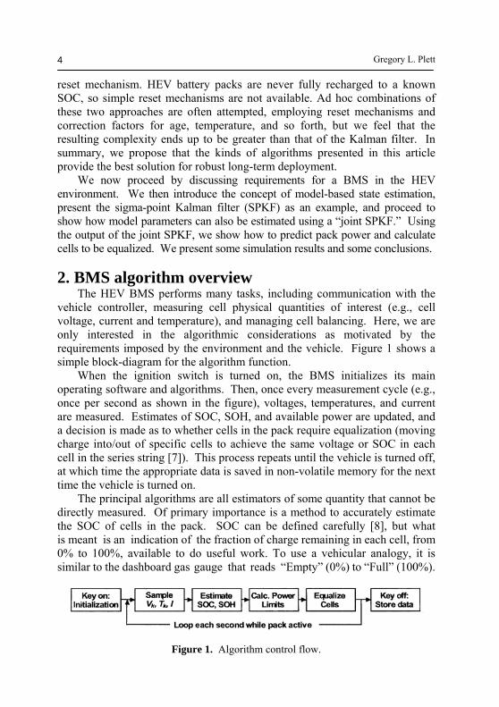
2. BMS algorithm overview The HEV BMS performs many tasks, including communication with the vehicle controller, measuring cell physical quantities of interest (e.g., cell voltage, current and temperature), and managing cell balancing. Here, we are only interested in the algorithmic considerations as motivated by the requirements imposed by the environment and the vehicle. Figure 1 shows a simple block-diagram for the algorithm function. When the ignition switch is turned on, the BMS initializes its main operating software and algorithms. Then, once every measurement cycle (e.g., once per second as shown in the figure), voltages, temperatures, and current are measured. Estimates of SOC, SOH, and available power are updated, and a decision is made as to whether cells in the pack require equalization (moving charge into/out of specific cells to achieve the same voltage or SOC in each cell in the series string [7]). This process repeats until the vehicle is turned off, at which time the appropriate data is saved in non-volatile memory for the next time the vehicle is turned on. The principal algorithms are all estimators of some quantity that cannot be directly measured. Of primary importance is a method to accurately estimate the SOC of cells in the pack. SOC can be defined carefully [8], but what is meant is an indication of the fraction of charge remaining in each cell, from 0% to 100%, available to do useful work. To use a vehicular analogy, it is similar to the dashboard gas gauge that reads “Empty” (0%) to “Full” (100%).

Figure 1. Algorithm control flow.

BMS algorithms for HEV SOC and SOH estimation 5

However, while there exist sensors to accurately measure a gasoline level in a tank, there is no sensor available to measure SOC. Further, precise SOC estimates provide the following benefits [9]: • Longevity: If a gasoline tank is over-filled or run empty, no harm is done

to the tank. However, over-charging or over-discharging a battery cell may cause permanent damage and result in reduced lifetime. An accurate SOC estimate may be used to avoid harming cells by not permitting current to be passed that would cause damage.

• Performance: Without a good SOC estimator, one must be overly conservative when using the battery pack to avoid over/undercharge due to trusting the poor estimate. With a good estimate, especially one with known error bounds, one can aggressively use the entire pack capacity.

• Reliability: A poor SOC estimator behaves differently for different driving profiles. A good SOC estimator is constant and dependable, enhancing overall power system reliability.

• Density: Accurate SOC and battery state information allows the battery pack to be used aggressively within the design limits, so the pack does not need to be over-engineered. This allows smaller, lighter battery packs.

• Economy: Smaller battery systems cost less. Warranty service on a reliable system costs less.

Knowledge of battery state of health (SOH) is also required. SOH is partially described by diagnostic flags including simple measurements such as: “Does any voltage/ current/ temperature measurement exceed design limits”? Complete SOH estimation also requires more complex estimation: “Are there any cells with SOC above or below design limits”? “Are there any cells with self-discharge rate above some acceptable limit”? “Has the capacity of any cell faded below some minimum acceptable value”? “Does the internal resistance of any cell exceed some limit”? and so forth. The pack may be serviced when SOH is not acceptable; SOH information may also be written to a data log for warranty purposes. In this article, we describe SOC/SOH estimators based on joint sigma-point Kalman filtering. These, in turn, are based on the framework of model-based estimation, which is introduced in the next section. 3. Model-based estimation All forms of model-based estimation, of which the Kalman filter is one example, rely on a mathematical description of the dynamics governing the quantities being estimated. Here, we employ a “state-space” model of cell dynamics:

Gregory L. Plett 6

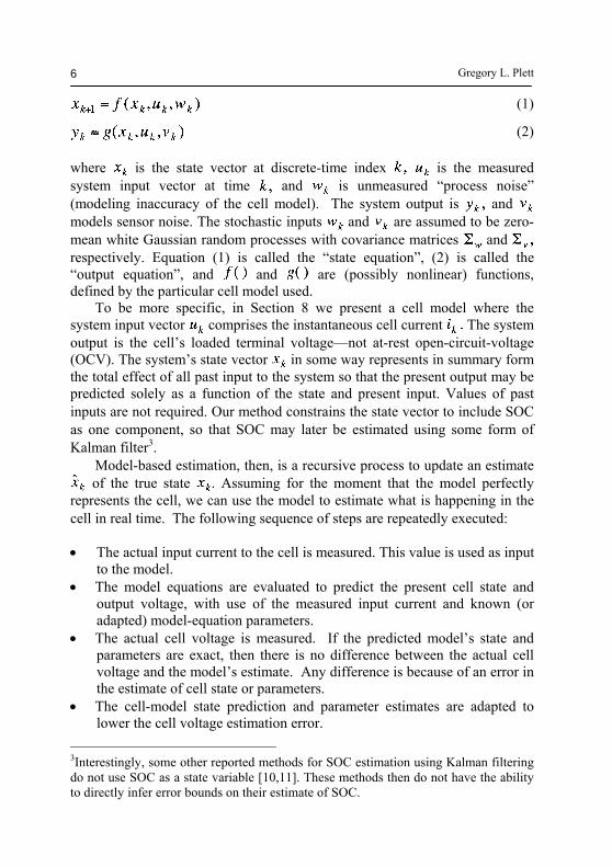
(1)

(2) where is the state vector at discrete-time index is the measured system input vector at time and is unmeasured “process noise” (modeling inaccuracy of the cell model). The system output is and models sensor noise. The stochastic inputs and are assumed to be zero-mean white Gaussian random processes with covariance matrices and respectively. Equation (1) is called the “state equation”, (2) is called the “output equation”, and and are (possibly nonlinear) functions, defined by the particular cell model used. To be more specific, in Section 8 we present a cell model where the system input vector comprises the instantaneous cell current The system output is the cell’s loaded terminal voltage—not at-rest open-circuit-voltage (OCV). The system’s state vector in some way represents in summary form the total effect of all past input to the system so that the present output may be predicted solely as a function of the state and present input. Values of past inputs are not required. Our method constrains the state vector to include SOC as one component, so that SOC may later be estimated using some form of Kalman filter3. Model-based estimation, then, is a recursive process to update an estimate

of the true state . Assuming for the moment that the model perfectly represents the cell, we can use the model to estimate what is happening in the cell in real time. The following sequence of steps are repeatedly executed: • The actual input current to the cell is measured. This value is used as input

to the model. • The model equations are evaluated to predict the present cell state and

output voltage, with use of the measured input current and known (or adapted) model-equation parameters.

• The actual cell voltage is measured. If the predicted model’s state and parameters are exact, then there is no difference between the actual cell voltage and the model’s estimate. Any difference is because of an error in the estimate of cell state or parameters.

• The cell-model state prediction and parameter estimates are adapted to lower the cell voltage estimation error.

____________________________

3Interestingly, some other reported methods for SOC estimation using Kalman filtering do not use SOC as a state variable [10,11]. These methods then do not have the ability to directly infer error bounds on their estimate of SOC.

BMS algorithms for HEV SOC and SOH estimation 7

• The updated state/parameter estimates are output to be used for whatever purposes are desired.

• This process repeats every sampling interval (e.g., every one second). This same approach works even when the cell model is not in fact perfect, or when there is noise on the sensors, but adaptation of the model’s state and parameter estimates must be made more slowly because of the additional uncertainty. In order to optimally perform the adaptation step, the algorithm must internally weigh uncertainties re. the model equations themselves, uncertainties re. the present state estimate, and uncertainties re. the values indicated by sensors. These are represented mathematically by covariance matrices of the appropriate variables. The variables themselves are understood to hold the expected value of the quantities that they represent. Since the algorithm must know these uncertainties, it has the added capability of being able to determine error bounds (for example, 3-sigma or 6-sigma error bounds) on all estimated quantities. To be more formal in our discussion of the steps of model-based estimation, we first define some notation. In the sequel, a superscript “–” denotes a predicted quantity, a superscript “+” denotes an updated estimate of that quantity, a circumflex “^” denotes an estimated quantity, a tilde “~” denotes an estimation error, and denotes the covariance of its subscripted variable. Further, we define to be the statistically expected value of its argument, and to be the history of measurements until time

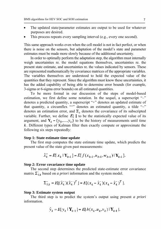
. Different types of Kalman filter then exactly compute or approximate the following six steps repeatedly: Step 1: State estimate time update The first step computes the state estimate time update, which predicts the present value of the state given past measurements:

Step 2: Error covariance time update The second step determines the predicted state-estimate error covariance matrix based on a priori information and the system model.

Step 3: Estimate system output The third step is to predict the system’s output using present a priori information.

Gregory L. Plett 8

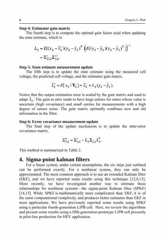
Step 4: Estimator gain matrix The fourth step is to compute the optimal gain factor used when updating the state estimate, which is

Step 5: State estimate measurement update The fifth step is to update the state estimate using the measured cell voltage, the predicted cell voltage, and the estimator gain matrix.

Notice that the output estimation error is scaled by the gain matrix and used to adapt The gain m atrix tends to have large entries for states whose value is uncertain (high covariance) and small entries for measurements with a high degree of sensor noise. The gain matrix optimally combines new and old information in the filter. Step 6: Error covariance measurement update The final step of the update mechanism is to update the state-error covariance matrix.

This method is summarized in Table 2.

4. Sigma-point kalman filters For a linear system, under certain assumptions, the six steps just outlined can be performed exactly. For a nonlinear system, they can only be approximated. The most common approach is to use an extended Kalman filter (EKF), and we have reported some results using this technique [12,8,13]. More recently, we have investigated another way to estimate these relationships for nonlinear systems—the sigma-point Kalman filter (SPKF) [14,15]. While SPKF is mathematically more complicated than EKF, it is of the same computational complexity, and produces better estimates than EKF in most applications. We have previously reported some results using SPKF using a particular fourth-generation LiPB cell. Here, we review the algorithms and present some results using a fifth-generation prototype LiPB cell presently in pilot-line production for HEV application.

BMS algorithms for HEV SOC and SOH estimation 9

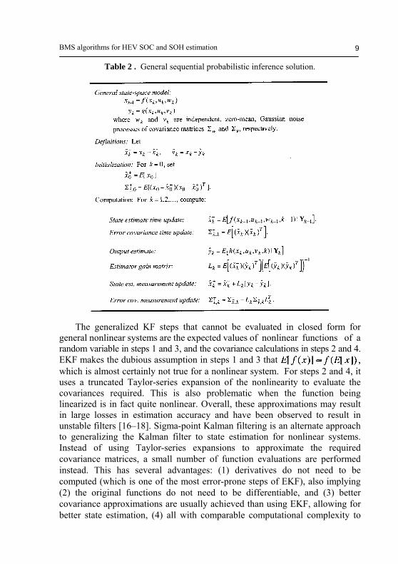
Table 2 . General sequential probabilistic inference solution.

The generalized KF steps that cannot be evaluated in closed form for general nonlinear systems are the expected values of nonlinear functions of a random variable in steps 1 and 3, and the covariance calculations in steps 2 and 4. EKF makes the dubious assumption in steps 1 and 3 that which is almost certainly not true for a nonlinear system. For steps 2 and 4, it uses a truncated Taylor-series expansion of the nonlinearity to evaluate the covariances required. This is also problematic when the function being linearized is in fact quite nonlinear. Overall, these approximations may result in large losses in estimation accuracy and have been observed to result in unstable filters [16–18]. Sigma-point Kalman filtering is an alternate approach to generalizing the Kalman filter to state estimation for nonlinear systems. Instead of using Taylor-series expansions to approximate the required covariance matrices, a small number of function evaluations are performed instead. This has several advantages: (1) derivatives do not need to be computed (which is one of the most error-prone steps of EKF), also implying (2) the original functions do not need to be differentiable, and (3) better covariance approximations are usually achieved than using EKF, allowing for better state estimation, (4) all with comparable computational complexity to

Gregory L. Plett 10

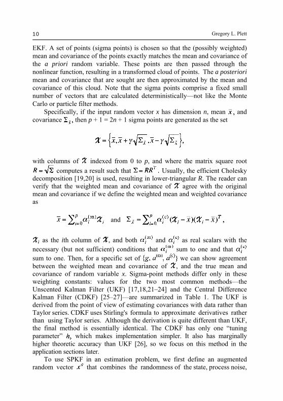
EKF. A set of points (sigma points) is chosen so that the (possibly weighted) mean and covariance of the points exactly matches the mean and covariance of the a priori random variable. These points are then passed through the nonlinear function, resulting in a transformed cloud of points. The a posteriori mean and covariance that are sought are then approximated by the mean and covariance of this cloud. Note that the sigma points comprise a fixed small number of vectors that are calculated deterministically—not like the Monte Carlo or particle filter methods. Specifically, if the input random vector x has dimension n, mean and covariance then p + 1 = 2n + 1 sigma points are generated as the set

with columns of indexed from 0 to p, and where the matrix square root

computes a result such that Usually, the efficient Cholesky decomposition [19,20] is used, resulting in lower-triangular R. The reader can verify that the weighted mean and covariance of agree with the original mean and covariance if we define the weighted mean and weighted covariance as

and

as the ith column of , and both and as real scalars with the necessary (but not sufficient) conditions that sum to one and that sum to one. Then, for a specific set of we can show agreement between the weighted mean and covariance of , and the true mean and covariance of random variable x. Sigma-point methods differ only in these weighting constants: values for the two most common methods—the Unscented Kalman Filter (UKF) [17,18,21–24] and the Central Difference Kalman Filter (CDKF) [25–27]—are summarized in Table 1. The UKF is derived from the point of view of estimating covariances with data rather than Taylor series. CDKF uses Stirling's formula to approximate derivatives rather than using Taylor series. Although the derivation is quite different than UKF, the final method is essentially identical. The CDKF has only one “tuning parameter” which makes implementation simpler. It also has marginally higher theoretic accuracy than UKF [26], so we focus on this method in the application sections later. To use SPKF in an estimation problem, we first define an augmented random vector that combines the randomness of the state, process noise,

BMS algorithms for HEV SOC and SOH estimation 11

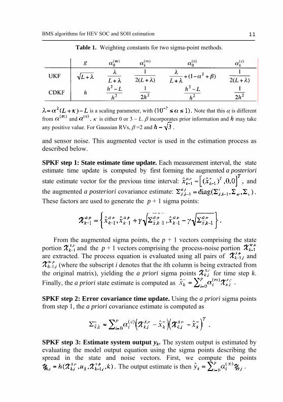
Table 1. Weighting constants for two sigma-point methods.

is a scaling parameter, with Note that this α is different from and κ is either 0 or 3 − L. β incorporates prior information and may take any positive value. For Gaussian RVs, β =2 and and sensor noise. This augmented vector is used in the estimation process as described below. SPKF step 1: State estimate time update. Each measurement interval, the state estimate time update is computed by first forming the augmented a posteriori state estimate vector for the previous time interval: and the augmented a posteriori covariance estimate: These factors are used to generate the p + 1 sigma points:

From the augmented sigma points, the p + 1 vectors comprising the state portion and the p + 1 vectors comprising the process-noise portion are extracted. The process equation is evaluated using all pairs of and

(where the subscript i denotes that the ith column is being extracted from the original matrix), yielding the a priori sigma points for time step k. Finally, the a priori state estimate is computed as SPKF step 2: Error covariance time update. Using the a priori sigma points from step 1, the a priori covariance estimate is computed as

SPKF step 3: Estimate system output yk. The system output is estimated by evaluating the model output equation using the sigma points describing the spread in the state and noise vectors. First, we compute the points

The output estimate is then

Gregory L. Plett 12

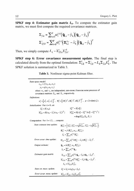
SPKF step 4: Estimator gain matrix Lk. To compute the estimator gain matrix, we must first compute the required covariance matrices.

Then, we simply compute SPKF step 6: Error covariance measurement update. The final step is calculated directly from the optimal formulation: The SPKF solution is summarized in Table 3.

Table 3. Nonlinear sigma-point Kalman filter.

BMS algorithms for HEV SOC and SOH estimation 13

5. Joint sigma-point filtering So far, we have assumed a constant cell model. However, when applying these procedures to estimate battery SOC, for example, we encounter a possible source of error: Not all cells are created equal; there is always some cell-to-cell variation, which only increases as the cells age, both in accumulated cycles and in calendar life. Some of the critical parameters, such as cell resistance and capacity, directly limit the pack performance through “power fade” and “capacity fade”. The state-of-health (SOH) of a battery is often described using these values. It is important to be able to estimate these and other parameters to: (1) maintain an accurate model for SOC estimation, and (2) understand the present battery state of health, and to predict remaining service life. Keeping in mind the previous discussion on estimating SOC, it is apparent that the quantities descriptive of the present battery pack condition exist on two time scales. Some change rapidly, such as SOC, which can traverse its entire range within minutes. Others may change very slowly, such as pack cell capacity, which might change as little as 20% in a decade or more of regular use. The quantities that tend to change quickly comprise the state of the system, and the quantities that tend to change slowly comprise the time-varying parameters of the system. The method used to estimate SOC can be modified to concurrently estimate both the quickly time-varying state and the slowly time-varying parameters by augmenting the cell model state vector with the model parameters and simultaneously estimating the values of this augmented state vector. This method is called joint estimation. A single filter combines the state and parameter estimates, so that both are adapted concurrently. Present state- and parameter-vector estimates are provided continuously as the electrochemical cell operates. This simple extension to standard SPKF is accomplished by revising the mathematical model of cell dynamics to explicitly include the parameters as the vector

Non-time-varying numeric values required by the model may be embedded within and and are not included in . To use the Enhanced Self-Correcting cell model from Section 8 as an example, the possibly time-varying parameters comprise the following: the Coulombic efficiency the total capacity C, the filter poles the filter weighting factors the cell discharge and charge resistances

Gregory L. Plett 14

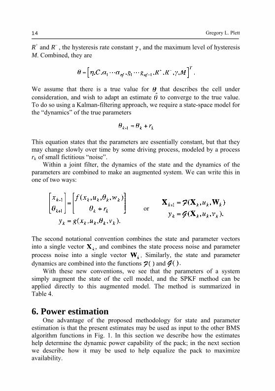
R+ and R− , the hysteresis rate constant and the maximum level of hysteresis M. Combined, they are

We assume that there is a true value for that describes the cell under consideration, and wish to adapt an estimate to converge to the true value. To do so using a Kalman-filtering approach, we require a state-space model for the “dynamics” of the true parameters

This equation states that the parameters are essentially constant, but that they may change slowly over time by some driving process, modeled by a process rk of small fictitious “noise”. Within a joint filter, the dynamics of the state and the dynamics of the parameters are combined to make an augmented system. We can write this in one of two ways:

or

The second notational convention combines the state and parameter vectors into a single vector and combines the state process noise and parameter process noise into a single vector Similarly, the state and parameter dynamics are combined into the functions and With these new conventions, we see that the parameters of a system simply augment the state of the cell model, and the SPKF method can be applied directly to this augmented model. The method is summarized in Table 4. 6. Power estimation One advantage of the proposed methodology for state and parameter estimation is that the present estimates may be used as input to the other BMS algorithm functions in Fig. 1. In this section we describe how the estimates help determine the dynamic power capability of the pack; in the next section we describe how it may be used to help equalize the pack to maximize availability.

BMS algorithms for HEV SOC and SOH estimation 15

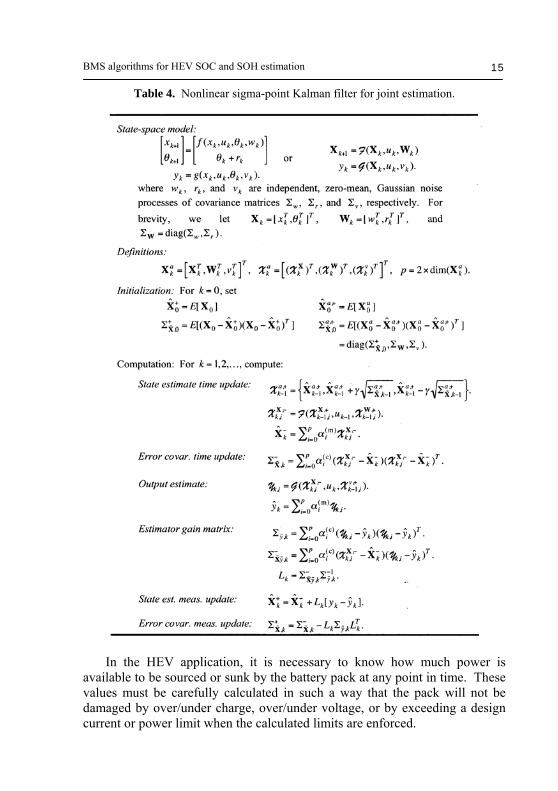
Table 4. Nonlinear sigma-point Kalman filter for joint estimation.

In the HEV application, it is necessary to know how much power is available to be sourced or sunk by the battery pack at any point in time. These values must be carefully calculated in such a way that the pack will not be damaged by over/under charge, over/under voltage, or by exceeding a design current or power limit when the calculated limits are enforced.

Gregory L. Plett 16

The power-estimation problem may be described as follows: Find the maximum battery charge and discharge power (based on present battery pack conditions) that may be maintained for m time samples without violating pre-set limits on cell voltage, state-of-charge, power, or current. Here, we denote the number of cells in the battery pack by N; cell voltage at time for cell number in the pack by which has operational design limits

similarly, state-of-charge has operational design limits cell power has operational design limits

and cell current by has operational design limits

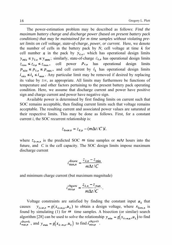
Any particular limit may be removed if desired by replacing its value by ±∞, as appropriate. All limits may furthermore be functions of temperature and other factors pertaining to the present battery pack operating condition. Here, we assume that discharge current and power have positive sign and charge current and power have negative sign. Available power is determined by first finding limits on current such that SOC remains acceptable, then finding current limits such that voltage remains acceptable. The resulting current and associated power values are saturated at their respective limits. This may be done as follows. First, for a constant current i, the SOC recurrent relationship is:

where is the predicted SOC time samples or hours into the future, and C is the cell capacity. The SOC design limits impose maximum discharge current

and minimum charge current (but maximum magnitude)

Voltage constraints are satisfied by finding the constant input that causes to obtain a design voltage, where is found by simulating (1) for time samples. A bisection (or similar) search algorithm [28] can be used to solve the relationship to find

and to find

BMS algorithms for HEV SOC and SOH estimation 17

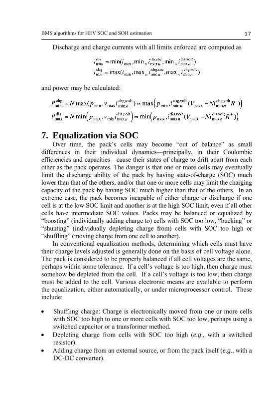
Discharge and charge currents with all limits enforced are computed as

and power may be calculated:

7. Equalization via SOC Over time, the pack’s cells may become “out of balance” as small differences in their individual dynamics—principally, in their Coulombic efficiencies and capacities—cause their states of charge to drift apart from each other as the pack operates. The danger is that one or more cells may eventually limit the discharge ability of the pack by having state-of-charge (SOC) much lower than that of the others, and/or that one or more cells may limit the charging capacity of the pack by having SOC much higher than that of the others. In an extreme case, the pack becomes incapable of either charge or discharge if one cell is at the low SOC limit and another is at the high SOC limit, even if all other cells have intermediate SOC values. Packs may be balanced or equalized by “boosting” (individually adding charge to) cells with SOC too low, “bucking” or “shunting” (individually depleting charge from) cells with SOC too high or “shuffling” (moving charge from one cell to another). In conventional equalization methods, determining which cells must have their charge levels adjusted is generally done on the basis of cell voltage alone. The pack is considered to be properly balanced if all cell voltages are the same, perhaps within some tolerance. If a cell’s voltage is too high, then charge must somehow be depleted from the cell. If a cell’s voltage is too low, then charge must be added to the cell. Various electronic means are available to perform the equalization, either automatically, or under microprocessor control. These include: • Shuffling charge: Charge is electronically moved from one or more cells

with SOC too high to one or more cells with SOC too low, perhaps using a switched capacitor or a transformer method.

• Depleting charge from cells with SOC too high (e.g., with a switched resistor).

• Adding charge from an external source, or from the pack itself (e.g., with a DC-DC converter).

Gregory L. Plett 18

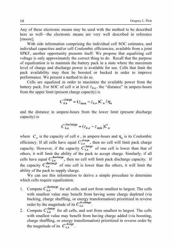
Any of these electronic means may be used with the method to be described here as well—the electronic means are very well described in reference [moore]. With side information comprising the individual cell SOC estimates, and individual capacities and/or cell Coulombic efficiencies, available from a joint SPKF, another opportunity presents itself. We propose that equalizing cell voltage is only approximately the correct thing to do. Recall that the purpose of equalization is to maintain the battery pack in a state where the maximum level of charge and discharge power is available for use. Cells that limit the pack availability may then be boosted or bucked in order to improve performance. We present a method to do so. Cells are equalized in order to maximize the available power from the battery pack. For SOC of cell n at level the “distance” in ampere-hours from the upper limit (present charge capacity) is

and the distance in ampere-hours from the lower limit (present discharge capacity) is

where is the capacity of cell n , in ampere-hours and is its Coulombic efficiency. If all cells have equal then no cell will limit pack charge capacity. However, if the capacity of one cell is lower than that of others, it will limit the ability of the pack to accept charge. Similarly, if all cells have equal then no cell will limit pack discharge capacity. If the capacity of one cell is lower than the others, it will limit the ability of the pack to supply charge. We can use this information to derive a simple procedure to determine which cells require equalization.

1. Compute for all cells, and sort from smallest to largest. The cells with smallest value may benefit from having some charge depleted (via bucking, charge shuffling, or energy transformation) prioritized in reverse order by the magnitude of its .

2. Compute for all cells, and sort from smallest to largest. The cells with smallest value may benefit from having charge added (via boosting, charge shuffling, or energy transformation) prioritized in reverse order by the magnitude of its .

BMS algorithms for HEV SOC and SOH estimation 19

3. If charge shuffling is available, it should be shuffled from the cells with minimum to cells with minimum , prioritized in reverse order by the corresponding magnitudes.

The SPKF may also contribute the estimation error bounds from the SOC estimate to help determine when to stop equalization. For example, one might turn off equalization if the difference between maximum and minimum

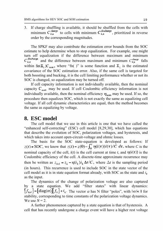
and the difference between maximum and minimum falls within where “fn( )” is some function and is the estimated covariance of the SOC estimation error. Also, if the same cell is targeted for both boosting and bucking, it is the cell limiting performance whether or not its SOC is changed, so equalization may be turned off. If cell capacity information is not individually available, then the nominal capacity may be used. If cell Coulombic efficiency information is not individually available, then the nominal efficiency may be used. If so, the procedure then equalizes SOC, which is not exactly the same as equalizing cell voltage. If all cell dynamic characteristics are equal, then the method becomes the same as equalizing by voltage. 8. ESC model The cell model that we use in this article is one that we have called the “enhanced self-correcting” (ESC) cell model [8,29,30], which has equations that describe the evolution of SOC, polarization voltages, and hysteresis, and which takes into account open-circuit-voltage and ohmic losses. The basis for the SOC state-equation is developed as follows: If

we know that where C is the nominal capacity of the cell, i(t) is the cell current at time t, and is the Coulombic efficiency of the cell. A discrete-time approximate recurrence may then be written as where ∆t is the sampling period (in hours). This recurrence is used to include SOC in the state vector of the cell model as it is in state equation format already, with SOC as the state and as the input. The dynamics of the change of polarization voltage are also captured by a state equation. We add “filter states” with linear dynamics:

The vector α has N filter “poles”, with for stability, corresponding to time constants of the polarization voltage dynamics. We use N = 2. A further phenomenon captured by a state equation is that of hysteresis. A cell that has recently undergone a charge event will have a higher rest voltage

Gregory L. Plett 20

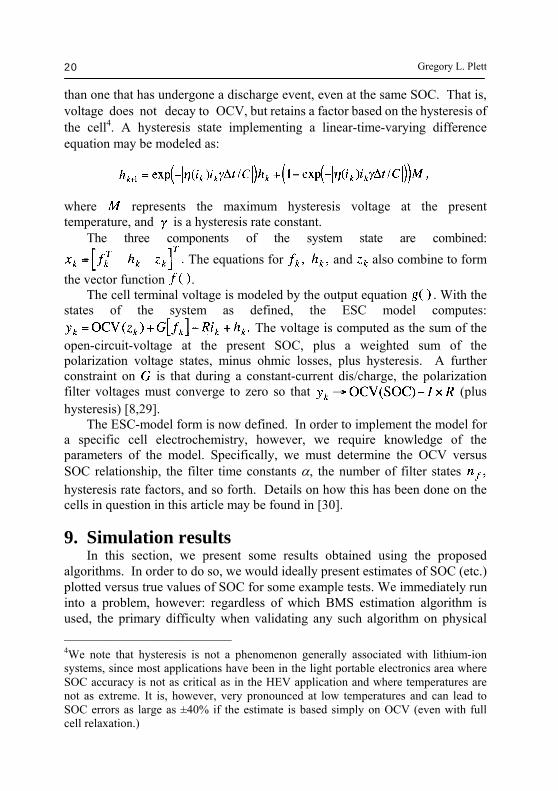
than one that has undergone a discharge event, even at the same SOC. That is, voltage does not decay to OCV, but retains a factor based on the hysteresis of the cell4. A hysteresis state implementing a linear-time-varying difference equation may be modeled as:

where represents the maximum hysteresis voltage at the present temperature, and is a hysteresis rate constant. The three components of the system state are combined:

The equations for and also combine to form the vector function . The cell terminal voltage is modeled by the output equation . With the states of the system as defined, the ESC model computes:

The voltage is computed as the sum of the open-circuit-voltage at the present SOC, plus a weighted sum of the polarization voltage states, minus ohmic losses, plus hysteresis. A further constraint on is that during a constant-current dis/charge, the polarization filter voltages must converge to zero so that (plus hysteresis) [8,29]. The ESC-model form is now defined. In order to implement the model for a specific cell electrochemistry, however, we require knowledge of the parameters of the model. Specifically, we must determine the OCV versus SOC relationship, the filter time constants α, the number of filter states hysteresis rate factors, and so forth. Details on how this has been done on the cells in question in this article may be found in [30].

9. Simulation results In this section, we present some results obtained using the proposed algorithms. In order to do so, we would ideally present estimates of SOC (etc.) plotted versus true values of SOC for some example tests. We immediately run into a problem, however: regardless of which BMS estimation algorithm is used, the primary difficulty when validating any such algorithm on physical _________________________

4We note that hysteresis is not a phenomenon generally associated with lithium-ion systems, since most applications have been in the light portable electronics area where SOC accuracy is not as critical as in the HEV application and where temperatures are not as extreme. It is, however, very pronounced at low temperatures and can lead to SOC errors as large as ±40% if the estimate is based simply on OCV (even with full cell relaxation.)

BMS algorithms for HEV SOC and SOH estimation 21

cells is that the “truth” values are not known. There are no sensors that can directly measure SOC, SOH, or available power. At different points in time, laboratory tests can be performed that can be used to determine a posteriori what the SOC/SOH/power was at that time, but cannot determine SOC/SOH/power in real time, as the battery pack operates. We have developed a simulation-based validation methodology as one component of a strategy that overcomes this obstacle [31]. A software simulator of cell dynamics first synthesizes various driving, temperature, parameter, and sensor-fault profiles for the battery pack being modeled. All internal variables that are dependent on the cycling history of the cell (e.g., SOC/ SOH/ power) are known to the software simulator, so “truth” values are established. The input-output behavior of this model has been tested against physical cells, and works well. We call this the “Data Generator System” (DGS). The BMS algorithms are then executed using this synthetic cell data as input, and the algorithm results are compared to the “truth” values.5 The synthesized data was generated using a model of a fifth-generation prototype LiPB cell that is very similar to the one presented in [14,15], but with a somewhat higher capacity. Root-mean-square (RMS) model error versus cell tests conducted using an Arbin BT2000 are on the order of 5–10 mV over all operating conditions. 9.1. Description of tests Figure 2 shows plots of the cell-current and cell-voltage profiles for the tests used to illustrate results. A single cell was simulated. The current profile comprises: first, a charge-neutral UDDS drive cycle, followed by a one-minute rest, a 2C charge for one minute, and another one minute rest; second, a charge-neutral US06 drive cycle, followed by a one-minute rest, a 4C discharge for one minute, and another one minute rest; third, a charge-neutral NYCC drive cycle, followed by a one minute rest. The maximum charge current was nearly 10C and the maximum discharge current was nearly 16C. This current profile was chosen to demonstrate that the algorithms work with a variety of excitation: realistic urban, highway, and mountainous drive cycles, rest intervals, and constant-current events. ______________________________ 5We acknowledge that this method is no substitute for actual testing of real cells. However, it can help to minimize the amount of this testing that is required if a careful design-of-experiments approach is taken. A balanced overall validation strategy therefore comprises a large suite of desktop validation tests and a smaller suite of real-time tests on physical battery packs. We present this “desktop validation” means here sine it gives an unequivocal truth value for the purpose of evaluating the algorithms themselves.

Gregory L. Plett 22

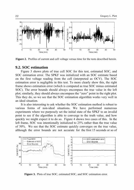
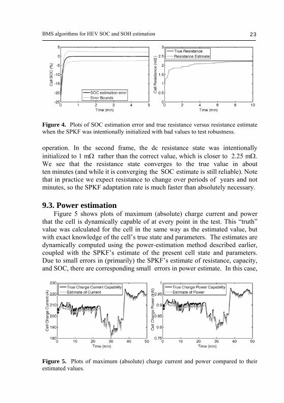
Figure 2. Profiles of current and cell voltage versus time for the tests described herein. 9.2. SOC estimation Figure 3 shows plots of true cell SOC for this test, estimated SOC, and SOC estimation error. The SPKF was initialized with an SOC estimate based on the first voltage reading from the cell (interpreted as OCV). The SOC estimation error is negligible in this test. To more clearly show this, the right frame shows estimation error (which is computed as true SOC minus estimated SOC). The error bounds should always encompass the true value in the left plot; similarly, they should always encompass the “zero” point in the right plot. This they do, so we see that the SOC estimation algorithm works very well in an ideal situation. It is also interesting to ask whether the SOC estimation method is robust to various forms of non-ideal situations. We have performed numerous experiments where we purposely set the initial state of the SPKF to an invalid point to see if the algorithm is able to converge to the truth value, and how quickly we might expect it to do so. Figure 4 shows two cases of this. In the left frame, SOC was intentionally initialized to 25% rather than the true value of 50%. We see that the SOC estimate quickly converges on the true value, although the error bounds are not accurate for the first 15 seconds or so of

Figure 3. Plots of true SOC, estimated SOC, and SOC estimation error.

BMS algorithms for HEV SOC and SOH estimation 23

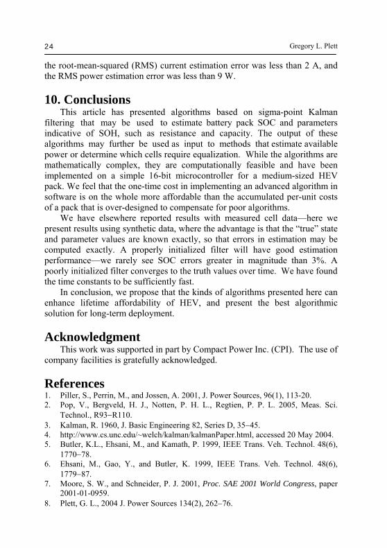
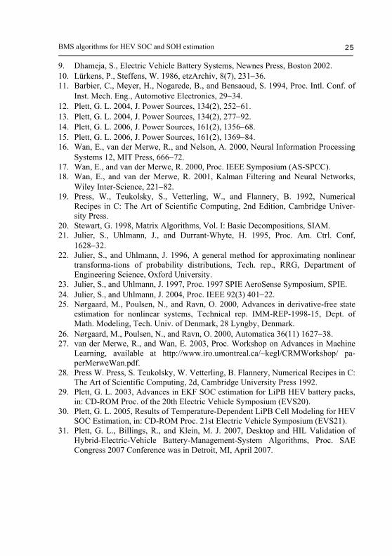
Figure 4. Plots of SOC estimation error and true resistance versus resistance estimate when the SPKF was intentionally initialized with bad values to test robustness. operation. In the second frame, the dc resistance state was intentionally initialized to 1 mΩ rather than the correct value, which is closer to 2.25 mΩ. We see that the resistance state converges to the true value in about ten minutes (and while it is converging the SOC estimate is still reliable). Note that in practice we expect resistance to change over periods of years and not minutes, so the SPKF adaptation rate is much faster than absolutely necessary. 9.3. Power estimation Figure 5 shows plots of maximum (absolute) charge current and power that the cell is dynamically capable of at every point in the test. This “truth” value was calculated for the cell in the same way as the estimated value, but with exact knowledge of the cell’s true state and parameters. The estimates are dynamically computed using the power-estimation method described earlier, coupled with the SPKF’s estimate of the present cell state and parameters. Due to small errors in (primarily) the SPKF’s estimate of resistance, capacity, and SOC, there are corresponding small errors in power estimate. In this case,

Figure 5. Plots of maximum (absolute) charge current and power compared to their estimated values.

Gregory L. Plett 24

the root-mean-squared (RMS) current estimation error was less than 2 A, and the RMS power estimation error was less than 9 W. 10. Conclusions This article has presented algorithms based on sigma-point Kalman filtering that may be used to estimate battery pack SOC and parameters indicative of SOH, such as resistance and capacity. The output of these algorithms may further be used as input to methods that estimate available power or determine which cells require equalization. While the algorithms are mathematically complex, they are computationally feasible and have been implemented on a simple 16-bit microcontroller for a medium-sized HEV pack. We feel that the one-time cost in implementing an advanced algorithm in software is on the whole more affordable than the accumulated per-unit costs of a pack that is over-designed to compensate for poor algorithms. We have elsewhere reported results with measured cell data—here we present results using synthetic data, where the advantage is that the “true” state and parameter values are known exactly, so that errors in estimation may be computed exactly. A properly initialized filter will have good estimation performance—we rarely see SOC errors greater in magnitude than 3%. A poorly initialized filter converges to the truth values over time. We have found the time constants to be sufficiently fast. In conclusion, we propose that the kinds of algorithms presented here can enhance lifetime affordability of HEV, and present the best algorithmic solution for long-term deployment. Acknowledgment This work was supported in part by Compact Power Inc. (CPI). The use of company facilities is gratefully acknowledged. References 1. Piller, S., Perrin, M., and Jossen, A. 2001, J. Power Sources, 96(1), 113-20. 2. Pop, V., Bergveld, H. J., Notten, P. H. L., Regtien, P. P. L. 2005, Meas. Sci.

Technol., R93−R110. 3. Kalman, R. 1960, J. Basic Engineering 82, Series D, 35−45. 4. http://www.cs.unc.edu/~welch/kalman/kalmanPaper.html, accessed 20 May 2004. 5. Butler, K.L., Ehsani, M., and Kamath, P. 1999, IEEE Trans. Veh. Technol. 48(6),

1770−78. 6. Ehsani, M., Gao, Y., and Butler, K. 1999, IEEE Trans. Veh. Technol. 48(6),

1779−87. 7. Moore, S. W., and Schneider, P. J. 2001, Proc. SAE 2001 World Congress, paper

2001-01-0959. 8. Plett, G. L., 2004 J. Power Sources 134(2), 262−76.

BMS algorithms for HEV SOC and SOH estimation 25

9. Dhameja, S., Electric Vehicle Battery Systems, Newnes Press, Boston 2002. 10. Lürkens, P., Steffens, W. 1986, etzArchiv, 8(7), 231−36. 11. Barbier, C., Meyer, H., Nogarede, B., and Bensaoud, S. 1994, Proc. Intl. Conf. of

Inst. Mech. Eng., Automotive Electronics, 29−34. 12. Plett, G. L. 2004, J. Power Sources, 134(2), 252−61. 13. Plett, G. L. 2004, J. Power Sources, 134(2), 277−92. 14. Plett, G. L. 2006, J. Power Sources, 161(2), 1356−68. 15. Plett, G. L. 2006, J. Power Sources, 161(2), 1369−84. 16. Wan, E., van der Merwe, R., and Nelson, A. 2000, Neural Information Processing

Systems 12, MIT Press, 666−72. 17. Wan, E., and van der Merwe, R. 2000, Proc. IEEE Symposium (AS-SPCC). 18. Wan, E., and van der Merwe, R. 2001, Kalman Filtering and Neural Networks,

Wiley Inter-Science, 221−82. 19. Press, W., Teukolsky, S., Vetterling, W., and Flannery, B. 1992, Numerical

Recipes in C: The Art of Scientific Computing, 2nd Edition, Cambridge Univer-sity Press.

20. Stewart, G. 1998, Matrix Algorithms, Vol. I: Basic Decompositions, SIAM. 21. Julier, S., Uhlmann, J., and Durrant-Whyte, H. 1995, Proc. Am. Ctrl. Conf,

1628−32. 22. Julier, S., and Uhlmann, J. 1996, A general method for approximating nonlinear

transforma-tions of probability distributions, Tech. rep., RRG, Department of Engineering Science, Oxford University.

23. Julier, S., and Uhlmann, J. 1997, Proc. 1997 SPIE AeroSense Symposium, SPIE. 24. Julier, S., and Uhlmann, J. 2004, Proc. IEEE 92(3) 401−22. 25. Nørgaard, M., Poulsen, N., and Ravn, O. 2000, Advances in derivative-free state

estimation for nonlinear systems, Technical rep. IMM-REP-1998-15, Dept. of Math. Modeling, Tech. Univ. of Denmark, 28 Lyngby, Denmark.

26. Nørgaard, M., Poulsen, N., and Ravn, O. 2000, Automatica 36(11) 1627−38. 27. van der Merwe, R., and Wan, E. 2003, Proc. Workshop on Advances in Machine

Learning, available at http://www.iro.umontreal.ca/~kegl/CRMWorkshop/ pa-perMerweWan.pdf.

28. Press W. Press, S. Teukolsky, W. Vetterling, B. Flannery, Numerical Recipes in C: The Art of Scientific Computing, 2d, Cambridge University Press 1992.

29. Plett, G. L. 2003, Advances in EKF SOC estimation for LiPB HEV battery packs, in: CD-ROM Proc. of the 20th Electric Vehicle Symposium (EVS20).

30. Plett, G. L. 2005, Results of Temperature-Dependent LiPB Cell Modeling for HEV SOC Estimation, in: CD-ROM Proc. 21st Electric Vehicle Symposium (EVS21).

31. Plett, G. L., Billings, R., and Klein, M. J. 2007, Desktop and HIL Validation of Hybrid-Electric-Vehicle Battery-Management-System Algorithms, Proc. SAE Congress 2007 Conference was in Detroit, MI, April 2007.