Bayes Decision Theory - II

Ken Kreutz-Delgado

Nuno Vasconcelos

ECE 175 – Winter 2011 - UCSD

2

Nearest Neighbor Classifier

• We are considering supervised classification

• Nearest Neighbor (NN) Classifier – A training set D = {(x1,y1), …, (xn,yn)}

– xi is a vector of observations, yi is the corresponding class label

– a vector x to classify

• The “NN Decision Rule” is – argmin means: “the i

that minimizes the distance”

*

{1,..., }

set

where

* arg min ( , )

i

ii n

y y

i d x x

3

Optimal Classifiers

• We have seen that performance depends on metric

• Some metrics are “better” than others

• The meaning of “better” is connected to how well adapted

the metric is to the properties of the data

• But can we be more rigorous? what do we mean by

optimal?

• To talk about optimality we define cost or loss

– Loss is the function that we want to minimize

– Loss depends on true y and prediction

– Loss tells us how good our predictor is

)(ˆ xfy x( )·f )ˆ,( yyL

y

4

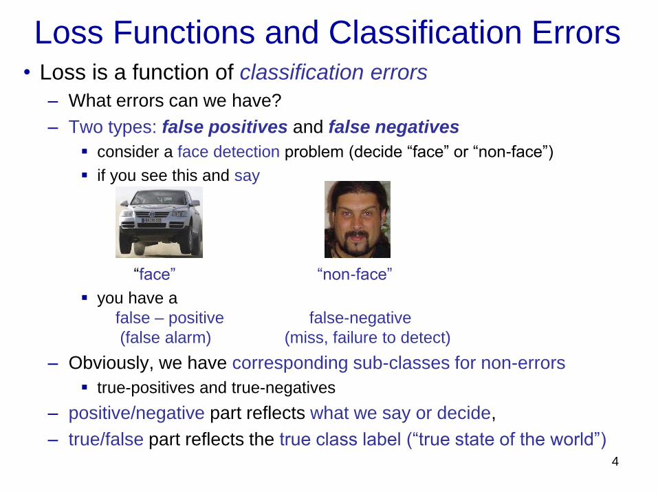
Loss Functions and Classification Errors • Loss is a function of classification errors

– What errors can we have?

– Two types: false positives and false negatives

consider a face detection problem (decide “face” or “non-face”)

if you see this and say

“face” “non-face”

you have a

false – positive false-negative

(false alarm) (miss, failure to detect)

– Obviously, we have corresponding sub-classes for non-errors

true-positives and true-negatives

– positive/negative part reflects what we say or decide,

– true/false part reflects the true class label (“true state of the world”)

5

(Conditional) Risk

• To weigh different errors differently

– We introduce a loss function

– Denote the cost of classifying X from class i as j by

– One way to measure how good the classifier is to use the

expected value of the loss, aka the (conditional) Risk,

– Note that the conditional risk is a function of both the class

decision, i, and the conditioning data (measured feature), x.

jiL

|( , ) ( | )Y X

j

R x i L j i P j x

6

Loss Functions

• example: two snakes and eating poisonous dart frogs

– Regular snake will die

– Frogs are a good snack for the

predator dart-snake

– This leads to the losses

– What is optimal decision when snakes

find a frog like these?

Regular

snake

dart

frog

regular

frog

regular 0

dart 0 10

Predator

snake

dart

frog

regular

frog

regular 10 0

dart 0 10

7

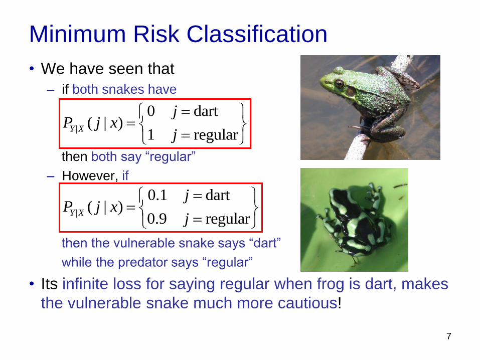
Minimum Risk Classification

• We have seen that

– if both snakes have

then both say “regular”

– However, if

then the vulnerable snake says “dart”

while the predator says “regular”

• Its infinite loss for saying regular when frog is dart, makes

the vulnerable snake much more cautious!

|

0.1 dart ( | )

0.9 regularY X

jP j x

j

|

0 dart ( | )

1 regularY X

jP j x

j

8

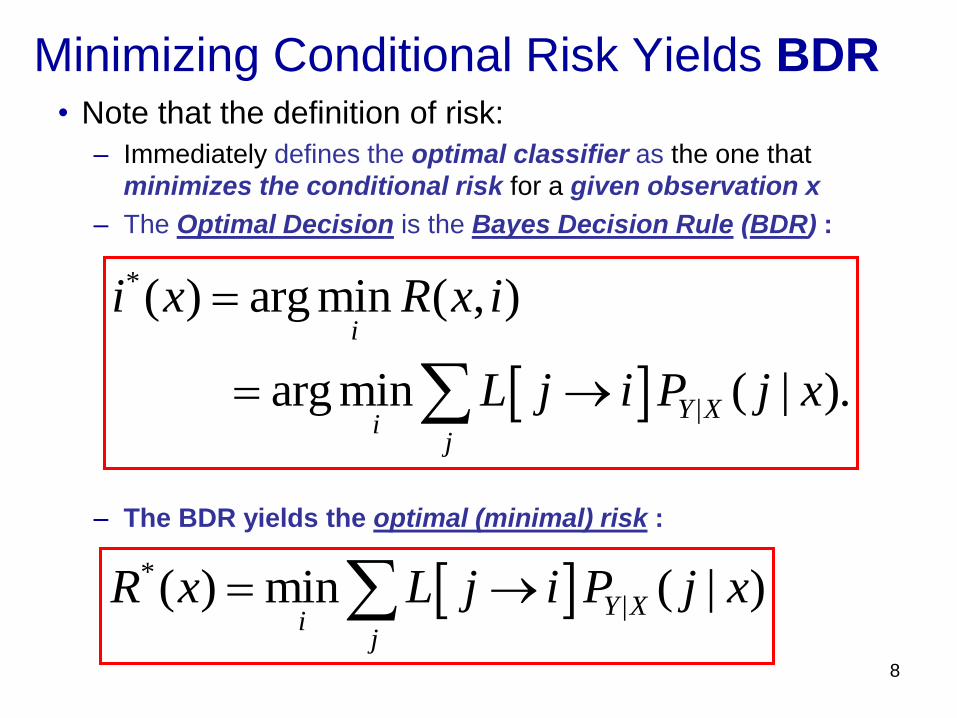
Minimizing Conditional Risk Yields BDR • Note that the definition of risk:

– Immediately defines the optimal classifier as the one that

minimizes the conditional risk for a given observation x

– The Optimal Decision is the Bayes Decision Rule (BDR) :

– The BDR yields the optimal (minimal) risk :

*

|

( ) arg min ( , )

arg min ( | ).

i

Y Xi

j

i x R x i

L j i P j x

*

|( ) min ( | )Y Xi

j

R x L j i P j x

What is a Decision Rule?

• Consider the c-ary classification problem with class labels,

• Given an observation (feature), x, to be classified, a

decision rule is a function d = d(.) of the observation that

takes its values in the set of class labels,

• Note that defined on the previous slide

is an optimal decision rule in the sense that for a specific

value of x it minimizes the conditional risk R(x,i) over all

possible decisions (classes) i in C

9

{1, , }.c

{1( ,) , }.cd x * *( ) ( )d x i x

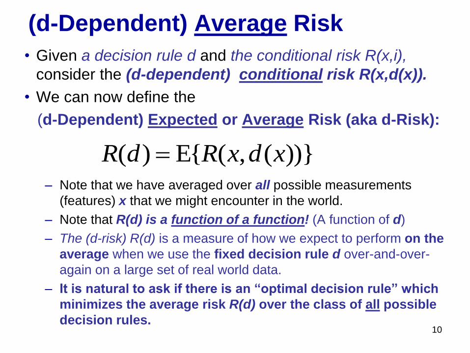
(d-Dependent) Average Risk

• Given a decision rule d and the conditional risk R(x,i),

consider the (d-dependent) conditional risk R(x,d(x)).

• We can now define the

(d-Dependent) Expected or Average Risk (aka d-Risk):

– Note that we have averaged over all possible measurements

(features) x that we might encounter in the world.

– Note that R(d) is a function of a function! (A function of d)

– The (d-risk) R(d) is a measure of how we expect to perform on the

average when we use the fixed decision rule d over-and-over-

again on a large set of real world data.

– It is natural to ask if there is an “optimal decision rule” which

minimizes the average risk R(d) over the class of all possible

decision rules. 10

( ) E ( , ){ ( })R d R x d x

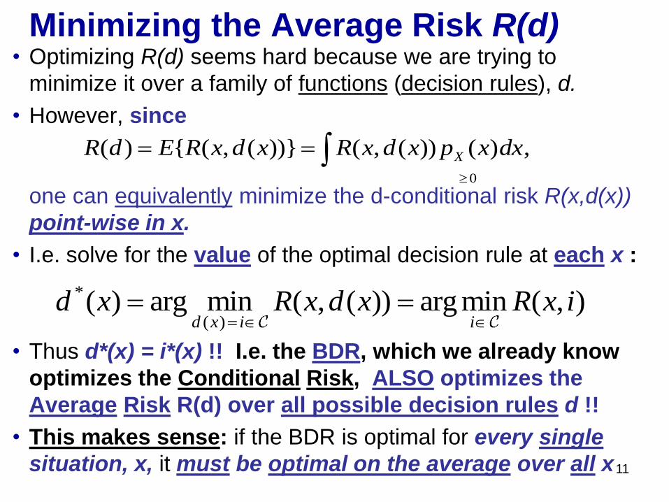
Minimizing the Average Risk R(d) • Optimizing R(d) seems hard because we are trying to

minimize it over a family of functions (decision rules), d.

• However, since

one can equivalently minimize the d-conditional risk R(x,d(x))

point-wise in x.

• I.e. solve for the value of the optimal decision rule at each x :

• Thus d*(x) = i*(x) !! I.e. the BDR, which we already know

optimizes the Conditional Risk, ALSO optimizes the

Average Risk R(d) over all possible decision rules d !!

• This makes sense: if the BDR is optimal for every single

situation, x, it must be optimal on the average over all x

11

0

( ) { ( , ( ))} ( , ( )) ( ) ,XR d E R x d x R x d x p x dx

*

( )( ) arg min ( , ( )) arg min ( , )

d x i ix R x d x Rd x i

12

The 0/1 Loss Function

• An important special case of interest:

– zero loss for no error and equal loss for two error types

• This is equivalent to the

“zero/one” loss :

• Under this loss the optimal Bayes decision rule (BDR) is

snake

prediction

dart

frog

regular

frog

regular 1 0

dart 0 1

ji

jijiL

1

0

|

* *

|

( ) arg min ( | )

arg min ( | )

( ) Y Xi

j

Y Xi

j i

d i x L j i P j

P

x x

j x

13

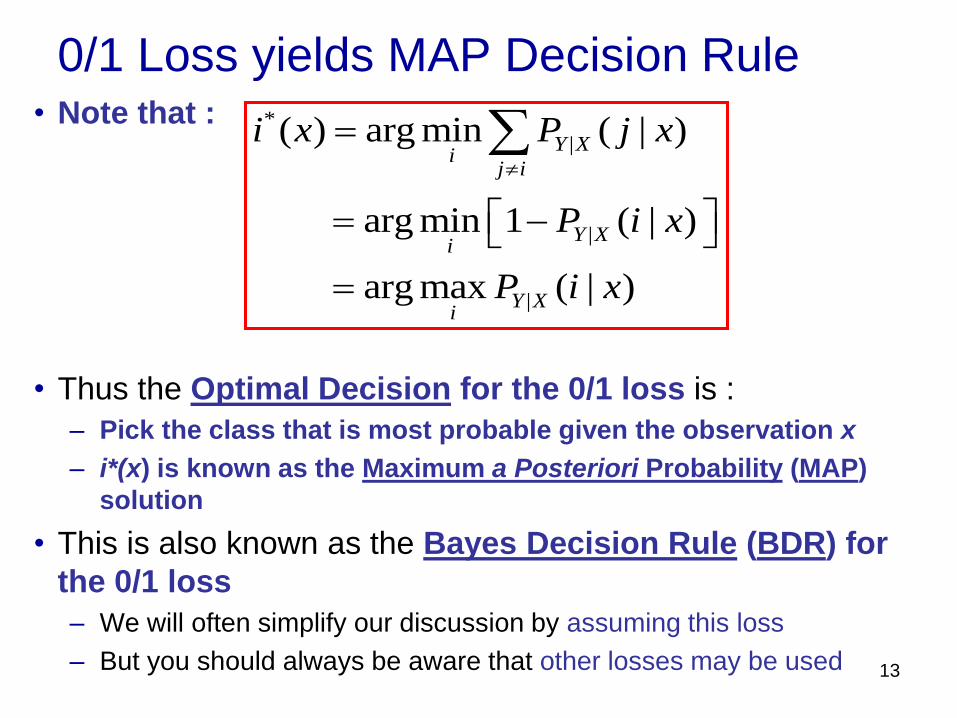
• Note that :

• Thus the Optimal Decision for the 0/1 loss is :

– Pick the class that is most probable given the observation x

– i*(x) is known as the Maximum a Posteriori Probability (MAP)

solution

• This is also known as the Bayes Decision Rule (BDR) for

the 0/1 loss

– We will often simplify our discussion by assuming this loss

– But you should always be aware that other losses may be used

*

|

|

|

( ) arg min ( | )

arg min 1 ( | )

arg max ( | )

Y Xi

j i

Y Xi

Y Xi

i x P j x

P i x

P i x

0/1 Loss yields MAP Decision Rule

14

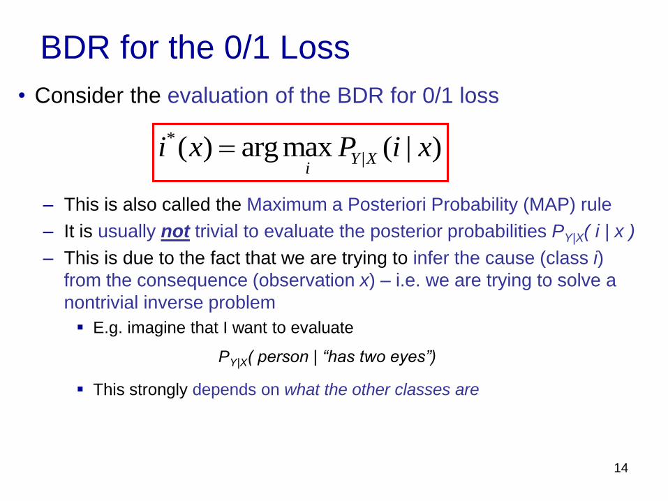
BDR for the 0/1 Loss

• Consider the evaluation of the BDR for 0/1 loss

– This is also called the Maximum a Posteriori Probability (MAP) rule

– It is usually not trivial to evaluate the posterior probabilities PY|X( i | x )

– This is due to the fact that we are trying to infer the cause (class i)

from the consequence (observation x) – i.e. we are trying to solve a

nontrivial inverse problem

E.g. imagine that I want to evaluate

PY|X( person | “has two eyes”)

This strongly depends on what the other classes are

*

|( ) arg max ( | )Y Xi

i x P i x

15

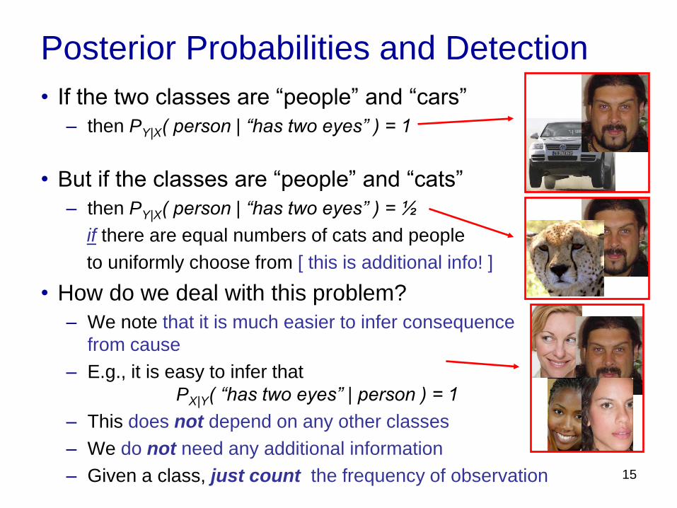
Posterior Probabilities and Detection

• If the two classes are “people” and “cars”

– then PY|X( person | “has two eyes” ) = 1

• But if the classes are “people” and “cats”

– then PY|X( person | “has two eyes” ) = ½

if there are equal numbers of cats and people

to uniformly choose from [ this is additional info! ]

• How do we deal with this problem?

– We note that it is much easier to infer consequence

from cause

– E.g., it is easy to infer that

PX|Y( “has two eyes” | person ) = 1

– This does not depend on any other classes

– We do not need any additional information

– Given a class, just count the frequency of observation

16

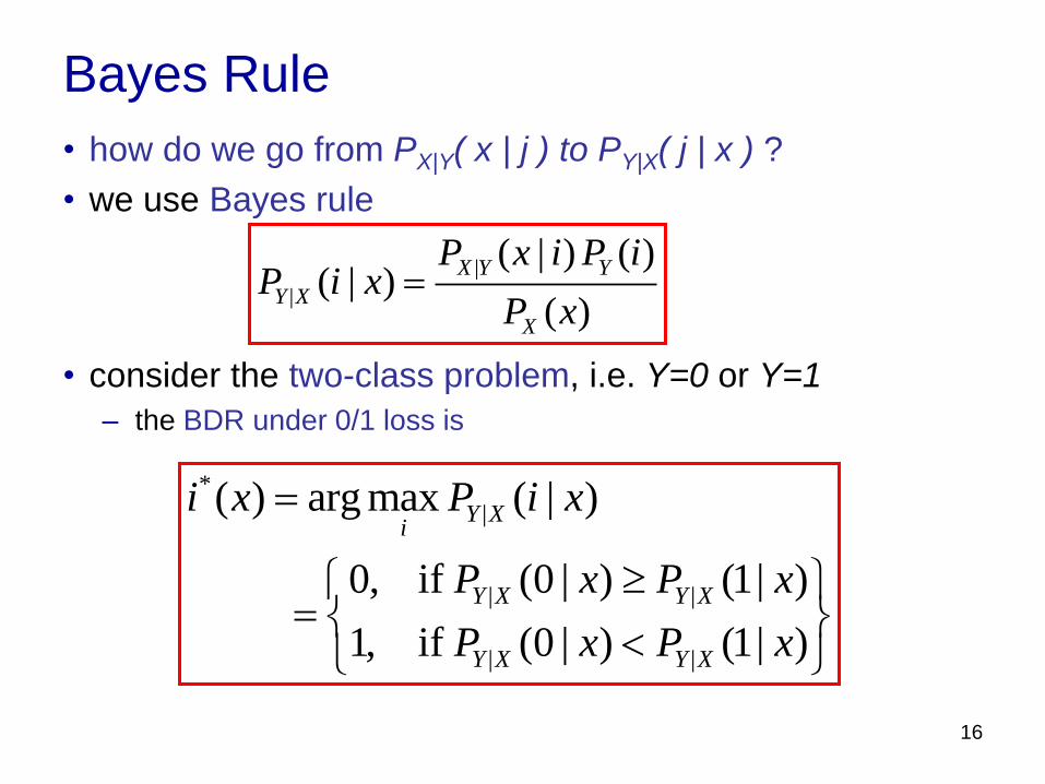
Bayes Rule

• how do we go from PX|Y( x | j ) to PY|X( j | x ) ?

• we use Bayes rule

• consider the two-class problem, i.e. Y=0 or Y=1

– the BDR under 0/1 loss is

|

|

( | ) ( )( | )

( )

X Y Y

Y X

X

P x i P iP i x

P x

*

|

| |

| |

( ) arg max ( | )

0, if (0 | ) (1| )

1, if (0 | ) (1| )

Y Xi

Y X Y X

Y X Y X

i x P i x

P x P x

P x P x

17

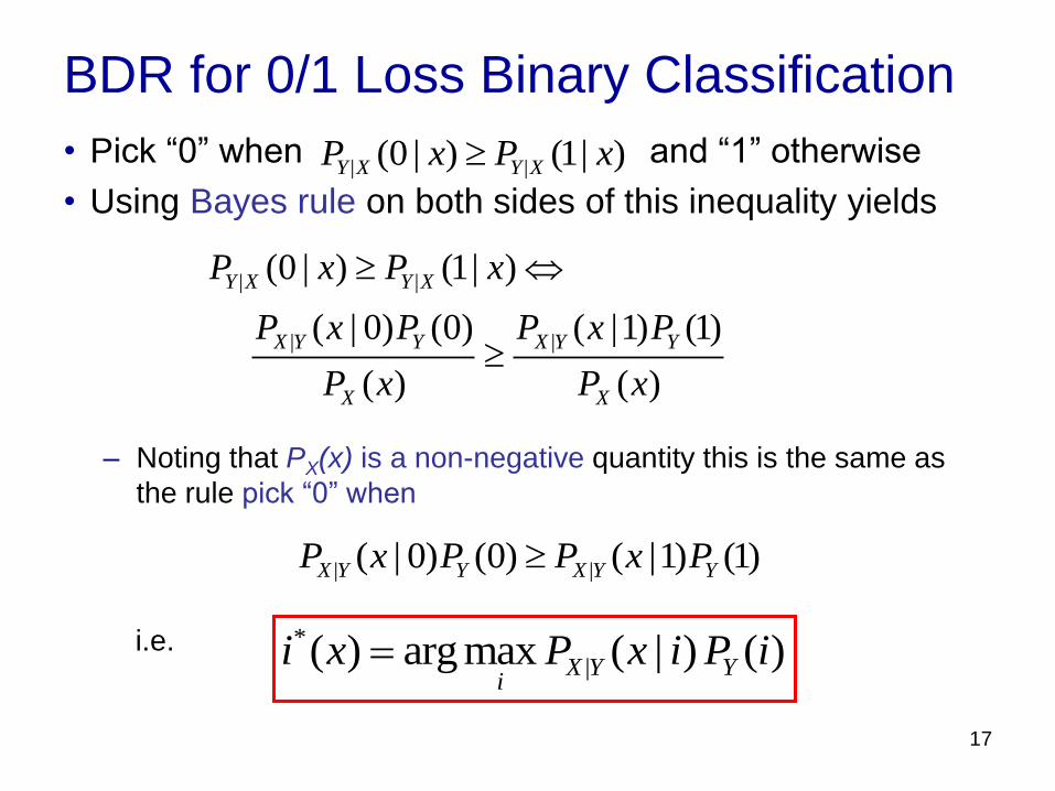
BDR for 0/1 Loss Binary Classification

• Pick “0” when and “1” otherwise

• Using Bayes rule on both sides of this inequality yields

– Noting that PX(x) is a non-negative quantity this is the same as

the rule pick “0” when

i.e.

| |(0 | ) (1| )Y X Y XP x P x

| |

| |

(0 | ) (1| )

( | 0) (0) ( |1) (1)

( ) ( )

Y X Y X

X Y Y X Y Y

X X

P x P x

P x P P x P

P x P x

| |( | 0) (0) ( |1) (1)X Y Y X Y YP x P P x P

*

|( ) arg max ( | ) ( )X Y Yi

i x P x i P i

18

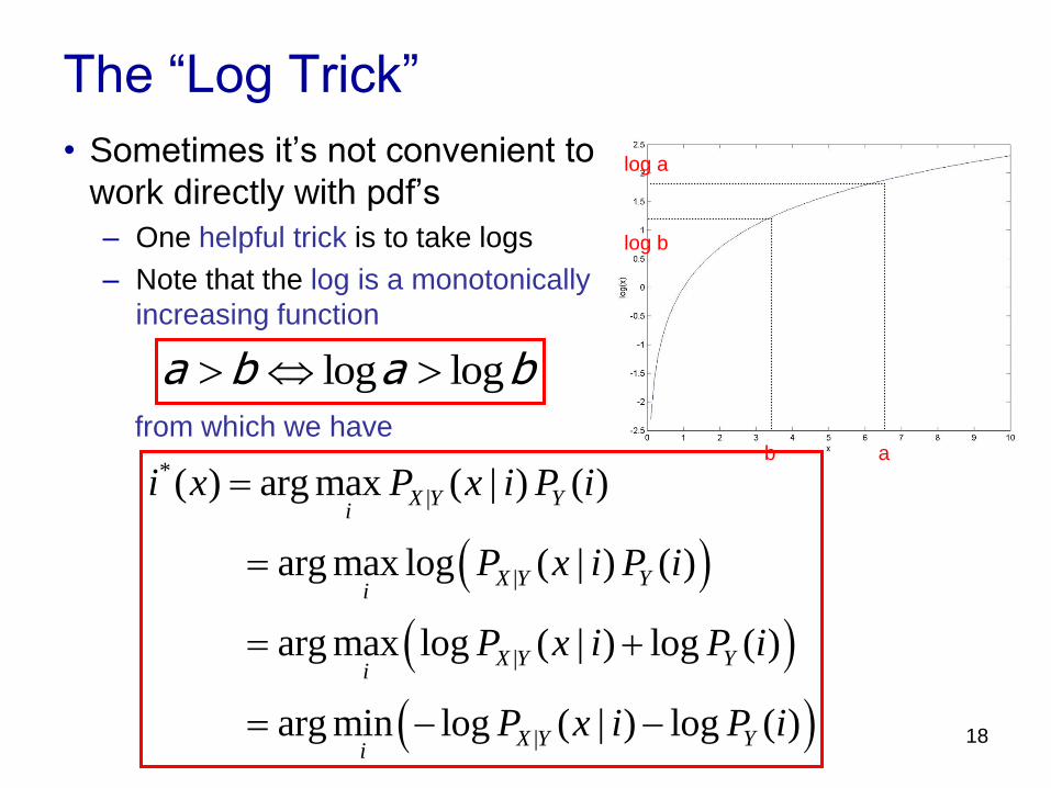
The “Log Trick”

• Sometimes it’s not convenient to

work directly with pdf’s

– One helpful trick is to take logs

– Note that the log is a monotonically

increasing function

from which we have

baba loglog

a b

log b

log a

*

|

|

|

|

( ) arg max ( | ) ( )

arg max log ( | ) ( )

arg max log ( | ) log ( )

arg min log ( | ) log ( )

X Y Yi

X Y Yi

X Y Yi

X Y Yi

i x P x i P i

P x i P i

P x i P i

P x i P i

19

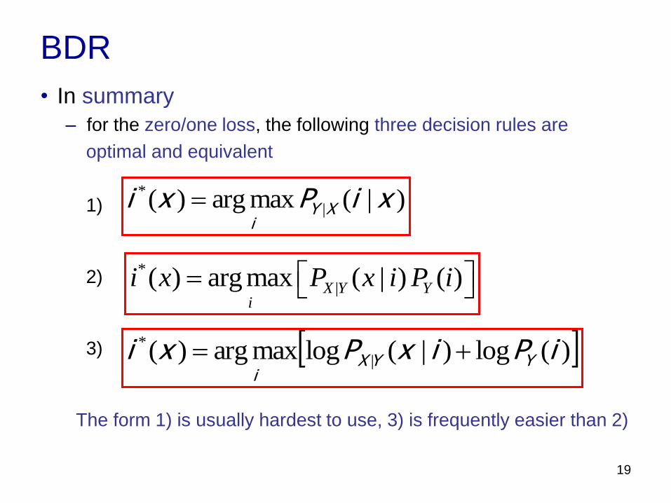
BDR

• In summary

– for the zero/one loss, the following three decision rules are

optimal and equivalent

1)

2)

3)

The form 1) is usually hardest to use, 3) is frequently easier than 2)

)|(maxarg)( |

* xiPxi XYi

*

|( ) arg max ( | ) ( )X Y Yi

i x P x i P i

)(log)|(logmaxarg)( |

* iPixPxi YYXi

20

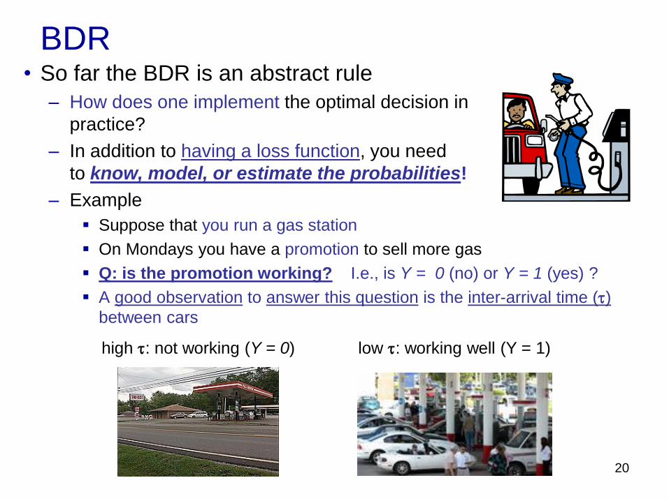
BDR • So far the BDR is an abstract rule

– How does one implement the optimal decision in

practice?

– In addition to having a loss function, you need

to know, model, or estimate the probabilities!

– Example

Suppose that you run a gas station

On Mondays you have a promotion to sell more gas

Q: is the promotion working? I.e., is Y = 0 (no) or Y = 1 (yes) ?

A good observation to answer this question is the inter-arrival time (t)

between cars

high t: not working (Y = 0) low t: working well (Y = 1)

21

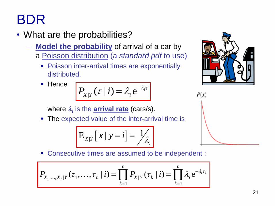
BDR • What are the probabilities?

– Model the probability of arrival of a car by

a Poisson distribution (a standard pdf to use)

Poisson inter-arrival times are exponentially

distributed.

Hence

where li is the arrival rate (cars/s).

The expected value of the inter-arrival time is

Consecutive times are assumed to be independent :

| ( | ) e i

X Y iP iltt l

|1E |X Y

i

x y il

1 , , | 1 |

1 1

( , , | ) ( | ) e i k

n

n n

X X Y n X Y ik

k k

P i P iltt t t l

22

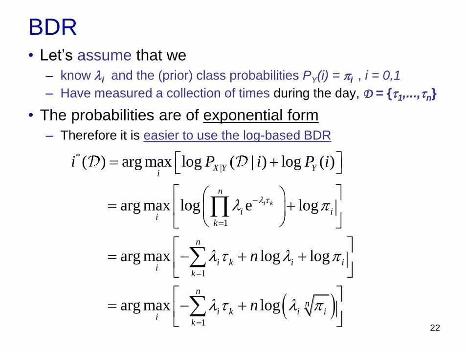
BDR • Let’s assume that we

– know li and the (prior) class probabilities PY(i) = pi , i = 0,1

– Have measured a collection of times during the day, D = {t1,...,tn}

• The probabilities are of exponential form

– Therefore it is easier to use the log-based BDR

*

|

1

1

1

( ) arg max log ( | ) log ( )

arg max log e log

arg max log log

arg max log

i k

X Y Yi

n

i ii

k

n

i k i ii

k

n

ni k i i

ik

i P i P i

n

n

l tl p

l t l p

l t l p

23

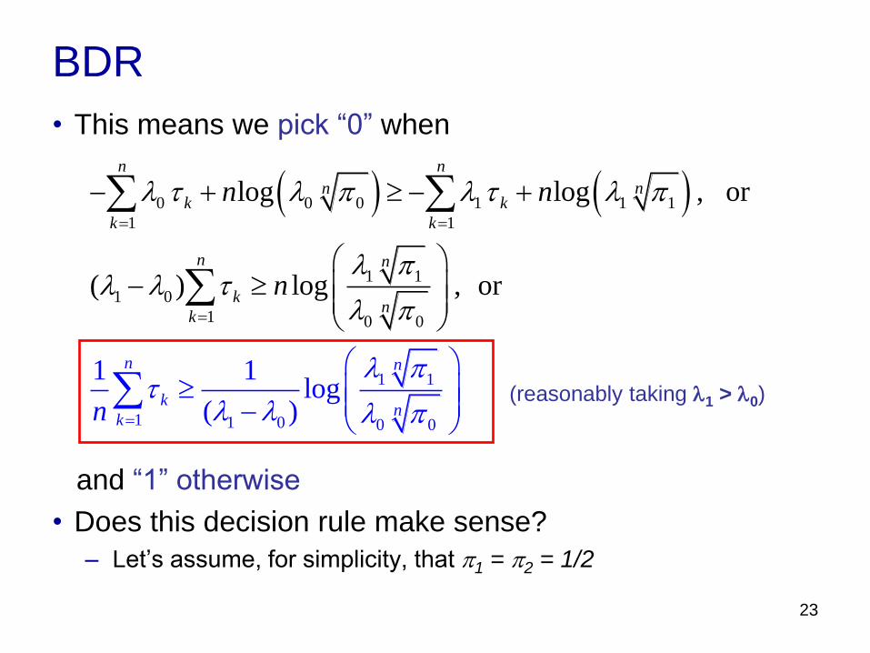
BDR

• This means we pick “0” when

and “1” otherwise

• Does this decision rule make sense?

– Let’s assume, for simplicity, that p1 = p2 = 1/2

0 0 0 1 1 1

1 1

1 1

1 0

1

1 1

1 1 0 0 0

0 0

log log

( ) lo

, or

, or

1 1log

( )

g

n n

k

n n

nnk k

k k

n n

k

n

nk

k

n n

n

n

l t l p l t l p

l

l pt

l

pl l

p

tl p

l l

(reasonably taking l1 > l0)

24

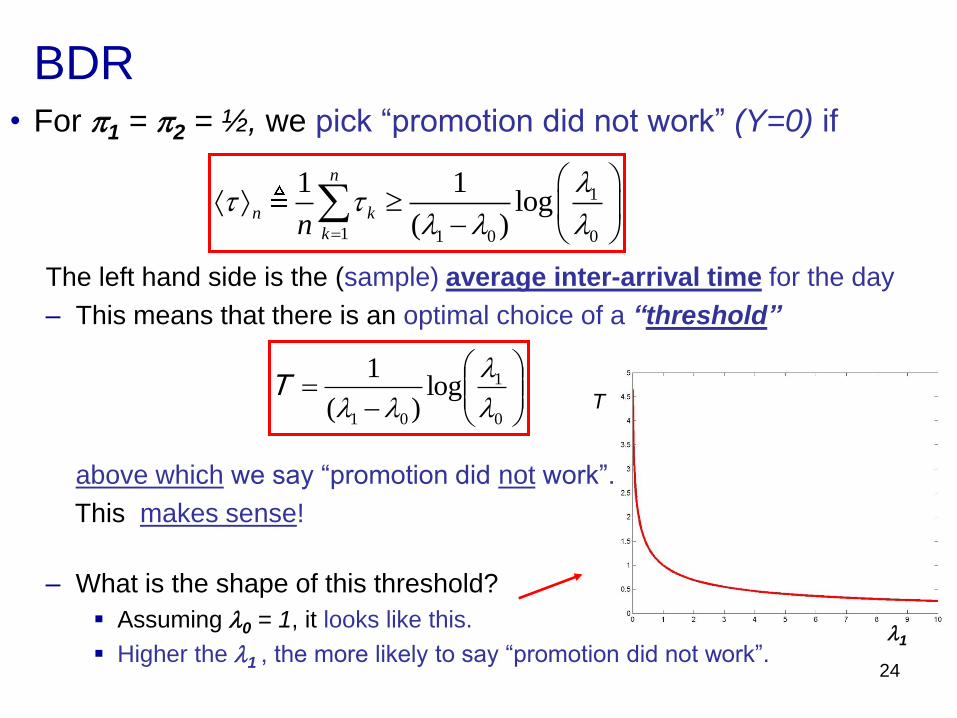
BDR • For p1 = p2 = ½, we pick “promotion did not work” (Y=0) if

The left hand side is the (sample) average inter-arrival time for the day

– This means that there is an optimal choice of a “threshold”

above which we say “promotion did not work”.

This makes sense!

– What is the shape of this threshold?

Assuming l0 = 1, it looks like this.

Higher the l1 , the more likely to say “promotion did not work”.

1

1 1 0 0

1 1log

( )

n

n k

kn

lt

l l lt

0

1

01

log)(

1

l

l

llT

l1

T

25

BDR • When p1 = p2 = ½, we pick “did not work” (Y=0) when

– Assuming l0 = 1, T decreases with l1

– I.e. for a given daily average,

Larger l1: easier to say “did not work”

– This means that

As the expected rate of arrival for good days increases

we are going to impose a tougher standard on the average

measured inter-arrival times

– The average has to be smaller for us to accept the day as a good one

– Once again, this makes sense!

– A sensible answer is usually the case with the BDR (a good way

to check your math)

1

1 n

k

k

n Tn

t t

0

1

01

log)(

1

l

l

llT

l1

T

26

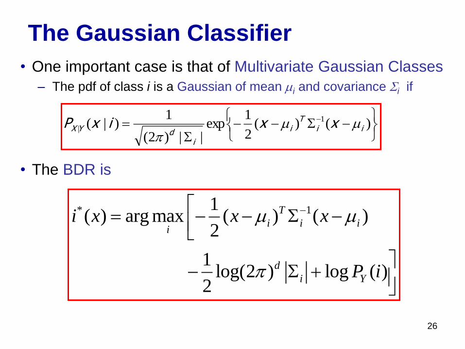
The Gaussian Classifier

• One important case is that of Multivariate Gaussian Classes

– The pdf of class i is a Gaussian of mean mi and covariance Si if

• The BDR is

SS

)()(2

1exp

||)2(

1)|( 1

| iiT

i

idYX xxixP mm

p

* 11( ) arg max ( ) ( )

2

1 log(2 ) log ( )

2

T

i i ii

d

i Y

i x x x

P i

m m

p

S

S

27

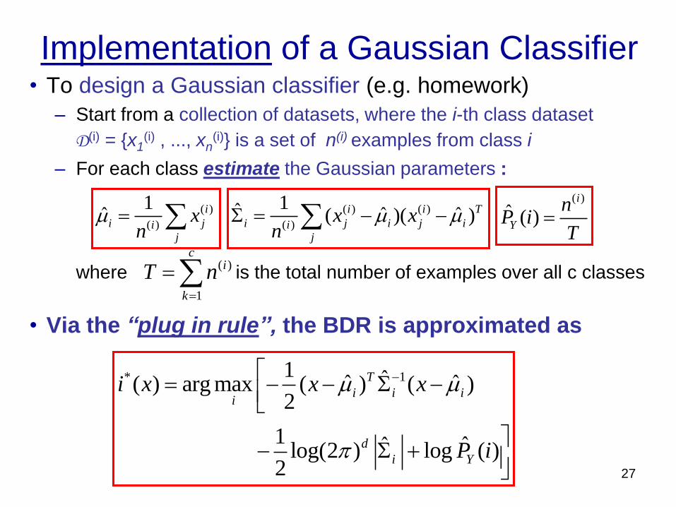
Implementation of a Gaussian Classifier • To design a Gaussian classifier (e.g. homework)

– Start from a collection of datasets, where the i-th class dataset

D(i) = {x1(i) , ..., xn

(i)} is a set of n(i) examples from class i

– For each class estimate the Gaussian parameters :

where is the total number of examples over all c classes

• Via the “plug in rule”, the BDR is approximated as

(

( ( )

)

)ˆ 1( )ˆ ( )ˆi i T

i ii j j

j

i x xn

m m S

1* 1( ) arg max ( ) ( )

2

1

ˆˆ ˆ

ˆˆ (log(2 ) l g )o2

T

ii i

d

i

i Y

i x

P

x x

ip

m m

S

S

( )

( )ˆ1 i

ij

i jxn

m ( )

ˆ ( )i

YT

in

P

( )

1

ci

k

nT

28

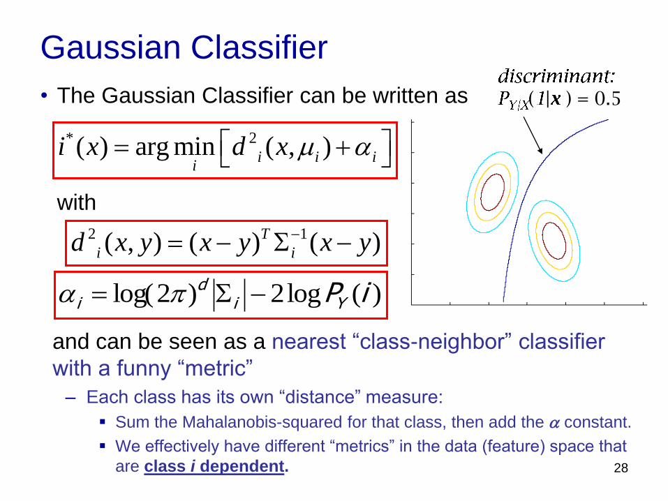
Gaussian Classifier

• The Gaussian Classifier can be written as

with

and can be seen as a nearest “class-neighbor” classifier

with a funny “metric”

– Each class has its own “distance” measure:

Sum the Mahalanobis-squared for that class, then add the a constant.

We effectively have different “metrics” in the data (feature) space that

are class i dependent.

2*( ) arg min ( , )i i ii

i x d x m a

12 ( , ) ( ) ( )T

i id x y x y x y S

)(log2)2log( iPYid

i S pa

( | ) = 0.5

29

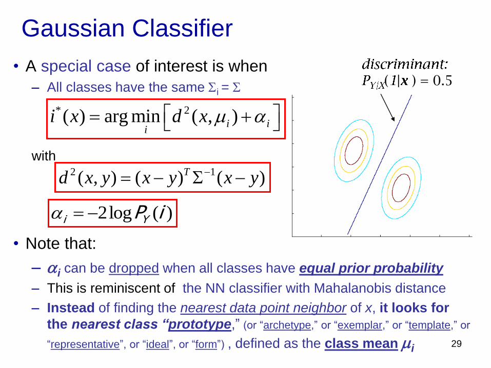
Gaussian Classifier

• A special case of interest is when

– All classes have the same Si = S

with

• Note that:

– ai can be dropped when all classes have equal prior probability

– This is reminiscent of the NN classifier with Mahalanobis distance

– Instead of finding the nearest data point neighbor of x, it looks for

the nearest class “prototype,” (or “archetype,” or “exemplar,” or “template,” or

“representative”, or “ideal”, or “form”) , defined as the class mean mi

2*( ) arg min ( , )i ii

i x d x m a

12 ( , ) ( ) ( )Td x y x y x y S

)(log2 iPYi a

( | ) = 0.5

30

Binary Classifier – Special Case

• Consider Si = S with two classes

– One important property of this case

is that the decision boundary is a

hyperplane (Homework)

– This can be shown by computing the

set of points x such that

and showing that they satisfy

which is the equation of a plane

with normal W that passes through

x0

0 0 1 1

2 2( , ) ( , )d x d xm a m a

( | ) = 0.5

0)( 0 xxw T

x 1

x 3 x 2

x n

w x0

x

x0

31

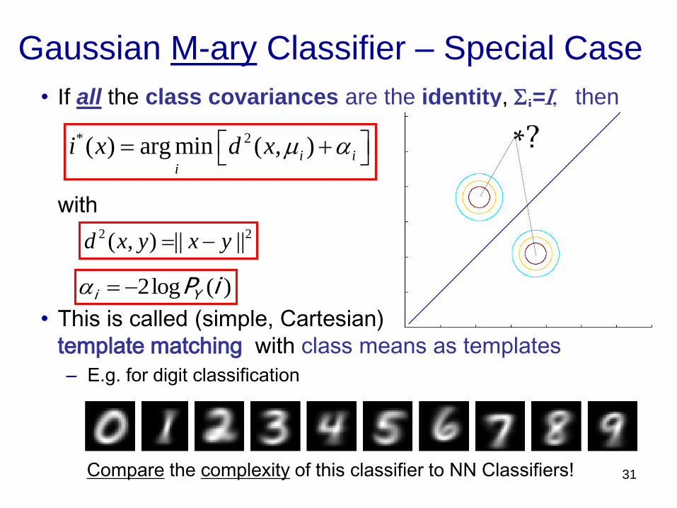
Gaussian M-ary Classifier – Special Case

• If all the class covariances are the identity, Si=I, then

with

• This is called (simple, Cartesian)

template matching with class means as templates

– E.g. for digit classification

Compare the complexity of this classifier to NN Classifiers!

2*( ) arg min ( , )i ii

i x d x m a

22 ( , ) || ||d x y x y

)(log2 iPYi a

* ?

32

The Sigmoid Function

• We have derived much of the above from the log-based BDR

• When there are only two classes, i = 0,1, it is also interesting

manipulate the original definition as follows:

where

*( ) arg max ( )ii

i x g x

*

|( ) arg max log ( | ) log ( )X Y Yi

i x P x i P i

|

|

|

| |

( | ) ( )( ) ( | )

( )

( | ) ( )

( | 0) (0) ( |1) (1)

X Y Y

i Y X

X

X Y Y

X Y Y X Y Y

P x i P ig x P i x

P x

P x i P i

P x P P x P

33

The Sigmoid Function

• Note that this can be written as

• For Gaussian classes, the posterior probabilities are

where, as before,

*( ) arg max ( )ii

i x g x0

|

|

1( )

( |1) (1)1

( | 0) (0)

X Y Y

X Y Y

g xP x P

P x P

)(1)( 01 xgxg

0

0 0 1 1 0 1

2 2

1( )

1 exp ( ) ( )g x

d x d xm m a a

12 ( , ) ( ) ( )T

i id x y x y x y S

)(log2)2log( iPYid

i S pa

34

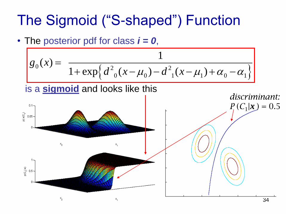
The Sigmoid (“S-shaped”) Function

• The posterior pdf for class i = 0,

is a sigmoid and looks like this

0

0 0 1 1 0 1

2 2

1( )

1 exp ( ) ( )g x

d x d xm m a a

( 1| ) = 0.5

35

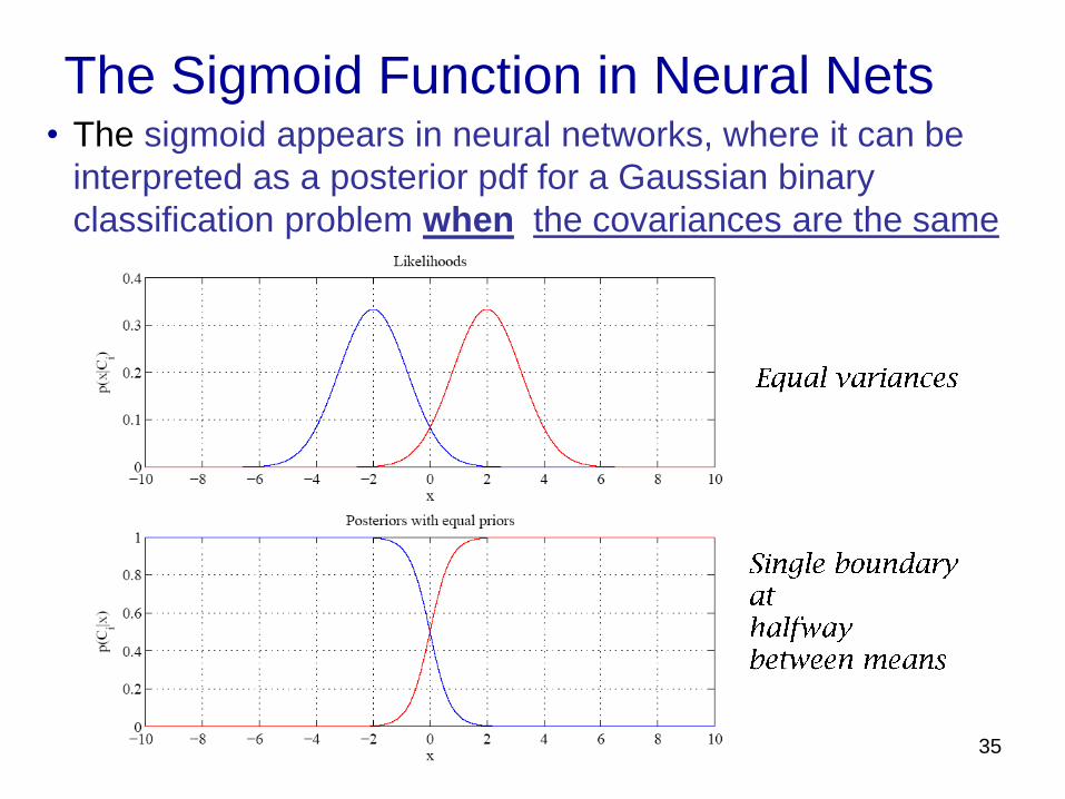
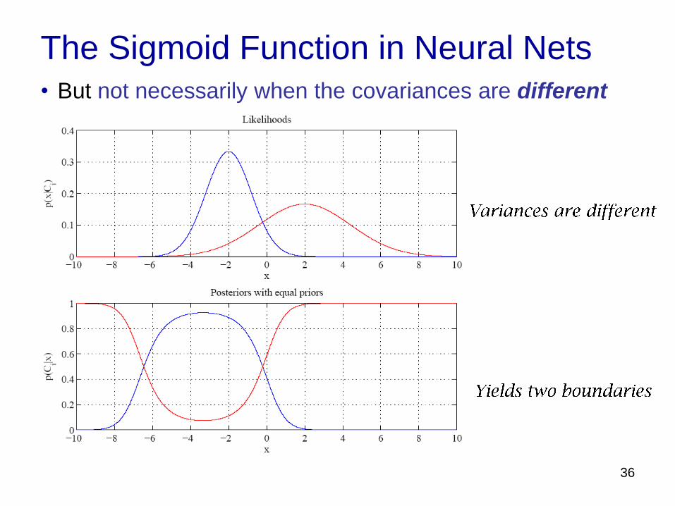
The Sigmoid Function in Neural Nets • The sigmoid appears in neural networks, where it can be

interpreted as a posterior pdf for a Gaussian binary

classification problem when the covariances are the same

36

The Sigmoid Function in Neural Nets • But not necessarily when the covariances are different

37

End