ISSN 1440-771X

Australia

Department of Econometrics and Business Statistics

http://www.buseco.monash.edu.au/depts/ebs/pubs/wpapers/

November 2011

Working Paper 24/11

Bayesian semiparametric GARCH models

Xibin Zhang and Maxwell L. King

Bayesian semiparametric GARCH models

Xibin Zhang1, Maxwell L. King

Department of Econometrics and Business Statistics, Monash University

November 3, 2011

Abstract: This paper aims to investigate a Bayesian sampling approach to parameter estima-

tion in the semiparametric GARCH model with an unknown conditional error density, which

we approximate by a mixture of Gaussian densities centered at individual errors and scaled by

a common standard deviation. This mixture density has the form of a kernel density estimator

of the errors with its bandwidth being the standard deviation. The proposed investigation is

motivated by the lack of robustness in GARCH models with any parametric assumption of

the error density for the purpose of error-density based inference such as value-at-risk (VaR)

estimation. The contribution of the paper is to construct the likelihood and posterior of model

and bandwidth parameters under the proposed mixture error density, and to forecast the

one-step out-of-sample density of asset returns. The resulting VaR measure therefore would

be distribution-free. Applying the semiparametric GARCH(1,1) model to daily stock-index

returns in eight stock markets, we find that this semiparametric GARCH model is favored

against the GARCH(1,1) model with Student t errors for five indices, and that the GARCH

model underestimates VaR compared to its semiparametric counterpart. We also investigate

the use and benefit of localized bandwidths in the proposed mixture density of the errors.

Key Words: Bayes factors, kernel-form error density, localized bandwidths, Markov chain

Monte Carlo, value-at-risk

JEL Classification: C11, C14, C15, G15

1Address: 900 Dandenong Road, Caulfield East, Victoria 3145, Australia. Telephone: +61-3-99032130.Fax: +61-3-99032007. Email: xibin.zhang@monash.edu.

1

1 Introduction

The autoregressive conditional heteroscedasticity (ARCH) model of Engle (1982) and the

generalized ARCH (GARCH) model of Bollerslev (1986) have proven to be very useful in

modelling volatilities of financial asset returns, and the assumption of conditional normality

of the error term has contributed to early successes of GARCH models. Weiss (1986) and

Bollerslev and Wooldridge (1992) showed that under the assumption of conditional normality

of the errors, the quasi maximum likelihood estimator (QMLE) of the vector of parameters

is consistent when the first two moments of the underlying GARCH process are correctly

specified. However, the Gaussian QMLE suffers from efficiency loss when the conditional error

density is non-Gaussian. Engle and González-Rivera (1991) investigated the efficiency loss of

the Gaussian QMLE through Monte Carlo simulations when the conditional error distribution

is non-Gaussian. In the literature on GARCH models, enough evidence found by theoretical

and empirical studies has shown that it is possible to reject the assumption of conditional

normality (Singleton and Wingender, 1986; Bollerslev, 1986; Badrinath and Chatterjee, 1988,

among others). This has motivated the investigation of other specifications of the conditional

distribution of errors in GARCH models, such as the Student t and other heavy-tailed densities

(see for example, Hall and Yao, 2003). In this paper, we aim to investigate the estimation

of parameters and error density in a GARCH model with an unknown error density. Our

investigation is motivated by the lack of robustness in a GARCH model with any parametric

assumption about its error density for the purpose of error-density based inference.

Engle and González-Rivera (1991) highlighted the importance of investigating the issue

of nonparametric estimation of the conditional density of errors at the same time when

parameters are estimated. They proposed a semiparametric GARCH model without any

assumption on the analytical form of error density. The error density was estimated by the

discrete maximum penalized likelihood estimate (DMPLE) of Tapia and Thompson (1978)

based on residuals, which were computed by applying either the ordinary least squares or

2

QMLE (under conditional normality) to the same model. The parameters of the semiparamet-

ric GARCH model were then estimated by maximizing the log-likelihood function constructed

through the estimated error density based on initially derived residuals. The Monte Carlo

simulation results obtained by Engle and González-Rivera (1991) showed that this semipara-

metric estimation approach could improve the efficiency of parameter estimates up to 50%

against QMLEs obtained under conditional normality. However, their likelihood function is

affected by initial parameter estimates, which might be inaccurate. Their semiparametric

estimation method uses the data twice because residuals have to be pre-fitted in order to

construct the likelihood. Moreover, the derived semiparametric estimates of parameters will

not be used again to improve the accuracy of the error density estimator.

This paper aims to investigate how we can simultaneously estimate the parameters and

conditional error density using information provided by the data without specifying the form

of the error density. It would be very attractive to impose minimal assumptions on the form

of error density in a GARCH model, because the resulting semiparametric model would gain

robustness in terms of specifications of the error density (see for example, Durham and

Geweke, 2011). In this situation, being able to estimate the error density is as important

as estimating parameters in the parametric component of the GARCH model because any

error-density-based inference would be robust with respect to specifications of error density.

Moreover, we can forecast the density of the underlying asset’s return. Let y = (y1, y2, . . . , yn)′

be a vector of n observations of an asset’s return. A GARCH(1,1) model is expressed as

yt =σt εt ,

σ2t =ω+αy2

t−1 +βσ2t−1, (1)

where εt , for t = 1,2, . . . ,n, are independent. It is often assumed that ω> 0, α≥ 0, β≥ 0 and

α+β< 1, and that conditional on information available at t −1 denoted as It−1, εt follows a

known distribution. Strictly speaking, we will never know the true density of εt . To estimate

parameters and make statistical inference, the error density is usually assumed to be of a

3

known form such as the standard Gaussian or Student t density. Any assumed density is

only an approximation to the true unknown error density. In this paper, we assume that the

unknown density of εt denoted as f (εt ), is approximated by a location-mixture density:

f (εt ;h) = 1

n

n∑j=1

1

hφ

(εt −ε j

h

), (2)

where φ(·) is the density of the standard Gaussian distribution. The Gaussian components

have a common variance h2 and different mean values at individual errors. From the view

of error-density specification, f (ε;h) is a well-defined probability density characterized by

h2. From the view of density estimation, f (εt ;h) is the kernel estimator of the error density

with φ(·) the kernel function and h the bandwidth. In terms of density estimation based on

directly observed data, Silverman (1978) proved the strong uniform consistency of the kernel

density estimator under some regularity conditions. Consequently, it is reasonable to expect

that conditional on model parameters, f (ε;h) approaches f (ε) as the sample size increases,

even though f (ε) has an unknown form. The performance of this kernel-form error density

would be only second to that of an oracle who knows the true error density. Most importantly,

the proposed kernel-form error density is completely determined by a single parameter, the

bandwidth or the standard deviation of the component Gaussians.

The location-mixture density given by (2) is actually the arithmetic mean of n density

functions of N (εi ,h2), for i = 1,2, . . . ,n. It is a well-defined density function with one param-

eter, which is the common variance of the component Gaussian densities. Therefore, from

a Bayesian’s view, conditional on the parameters that characterize the GARCH model, this

location-mixture density can be used to construct the likelihood and therefore, the posterior.

In the literature, the use of a scale-mixture density of Gaussian densities as the error density

in a regression model has been investigated with the Gaussian components usually assumed

to have a zero mean and different variances (see for example, Jensen and Maheu, 2010).

Therefore, the use of such a scale-mixture density is at the cost of dramatically increasing the

number of parameters. In contrast, our location-mixture error density places its locations at

4

the individual realized errors and has only one parameter, which we still call the bandwidth

due to its smoothing role.

Instead of using frequency approaches to investigate parameter estimation under an

unknown error density, we propose to derive an approximate posterior of the GARCH param-

eters and the bandwidths up to a normalizing constant, where the likelihood is approximated

through the location-mixture density of the errors. The priors of GARCH parameters are the

uniform density on (0,1), and the prior of the squared bandwidth is an inverse Gamma density.

Therefore, both types of parameters are estimable through Bayesian sampling.

Bayesian sampling techniques have been used to estimate parameters of a GARCH model

when the error density is specified (see for example, Bauwens and Lubrano, 1998; Nakatsuma,

2000; Vrontos, Dellaportas, and Politis, 2000). However, the posterior of the parameters, on

which those sampling methods were developed, is unavailable when the conditional density

of the errors is unknown. One contribution of this paper is to derive an approximate posterior

of the parameters through the proposed kernel-form conditional error density, which is

determined by the bandwidth parameter.

It is not rare to investigate Bayesian approaches to parameter estimation in a GARCH

model with an unspecified error density. To deal with the problem of possible misspecification

of the error density and impose inequality constraints on some parameters in the quasi

likelihood, Koop (1994) presented Bayesian semiparametric ARCH models, where the quasi

likelihood was constructed through a sequence of complicated polynomials. His finding

indicates that the use of Bayesian and semiparametric approaches to parameter estimation in

GARCH models is feasible and necessary. Our proposed Bayesian approach differs from his in

that we use a leave-one-out version of the kernel-form error density given by (2) to construct

the likelihood function, which is actually the full conditional composite likelihood (see for

example, Mardia, Kent, Hughes, and Taylor, 2009).

The proposed kernel-form error density is different from the kernel density estimator of

5

pre-fitted residuals, which is often used to construct a quasi likelihood for adaptive estimation

of parameters in many models including (G)ARCH models investigated by Linton (1993)

and Drost and Klaassen (1997). The conclusion drawn from their investigations is that

(G)ARCH parameters are approximately adaptively estimable. This type of estimation is often

conducted in a two-step procedure that uses the data twice. Di and Gangopadhyay (2011)

presented a semiparametric maximum likelihood estimator of parameters in GARCH models.

All those methods for the semiparametric GARCH model are based on pre-fitted residuals,

and therefore are second-stage methods. However, our kernel-form error density is a well-

defined probability density, which depends on the errors rather than the pre-fitted residuals.

Our proposed Bayesian sampling procedure is able to estimate the GARCH parameters and

bandwidth simultaneously.

Applying our proposed Bayesian sampling method to the semiparametric GARCH(1,1)

model of daily continuously compounded returns of the S&P 500 index, we find that according

to Bayes factors, this semiparametric model is favored with very strong evidence against the

GARCH(1,1) with Student t errors known as the t-GARCH(1,1) model. Although the estimate

of (α,β) derived under the semiparametric GARCH model is similar to that derived under

the t-GARCH model, the estimated density of the one-step out-of-sample return under the

semiparametric model is clearly different from the Student t density. Moreover, we find

that the proposed semiparametric model is favored with very strong evidence against the t-

GARCH(1,1) model for another three out of seven stock-index return series. In these situations,

the forecasted return densities under both models are clearly different from each other.

An important use of the estimated density of the one-step out-of-sample return derived

under the semiparametric GARCH model is to calculate the conditional value-at-risk (VaR),

and the resulting VaR would be robust in terms of different specifications of the error density

(Jorion, 1997, among others). We derive the VaRs for seven return series under the semipara-

metric model and its competing model, respectively. In comparison to the semiparametric

6

GARCH model, the t-GARCH model underestimates the conditional VaR for the four index

return series in the USA market.

We also investigate the issue of assigning different bandwidths to different realized errors

by incorporating their absolute values into the bandwidth. We find that the use of localized

bandwidths increases the competitiveness of our semiparametric GARCH model against the

t-GARCH model. Even though the use of localized bandwidths leads to a slightly smaller

VaR than that of a global bandwidth, the t-GARCH model still underestimates the VaR in

comparison to its semiparametric counterpart. This is a warning to any risk-avoiding financial

institution that uses the t-GARCH model for estimating conditional VaR.

The rest of the paper is organized as follows. In the next section, we discuss the validity and

benefit of the kernel-form error density and derive the posterior. In Section 3, we apply the

semiparametric GARCH(1,1) model to daily returns of the S&P 500 index, where Bayes factors

are used for model comparison, and VaRs are computed. Section 4 presents an empirical

study on the application of the semiparametric GARCH model to another seven index-return

series. In Section 5, we introduce localized bandwidths into the semiparametric GARCH

model, which is applied to the eight return series. Section 6 concludes the paper.

2 Bayesian estimation for the semiparametric GARCH model

2.1 A mixture of Gaussian densities

Let {x1, x2, . . . , xn} denote a sample of independent observations drawn from an unknown

probability density function g0(x;κ) with an unbounded support, where κ is the parameter

vector. In order to make statistical inference based on the sample, one has to make assump-

tions about the analytical form of g0(x;κ) based on some descriptive statistics such as the

histogram of the observations. Strictly speaking, any specification of the true density is only

an approximation to g (x;κ). One such approximation is given by

g (x;h) = 1

n

n∑i=1

1

hφ((x −xi )/h), (3)

7

which is a location-mixture density of n Gaussian components with the same variance h2 and

different mean values at individual observations. This mixture density is also known as the

kernel estimator of g0(x;κ), where φ(·) is the kernel function, and h is the bandwidth. From

the view of specifications of the underlying true density, this mixture density is a well-defined

density. Silverman (1978) proved that when h → 0, (nh)−1 lnn → 0 as n →∞, and g0(x;κ) is

uniformly continuous in x, g (x;h) is strongly uniformly consistent.

In this paper, we investigate how we can use this mixture density of Gaussian components

as an approximation to the unknown error density in a parametric regression model. Under

this assumption, a realization of this mixture density of the errors is equivalent to the kernel

density estimator of pre-fitted residuals, which is employed to construct a quasi likelihood for

adaptive estimation in the sense of Bickel (1982). Therefore, parameters can be estimated

by maximizing the quasi likelihood. One of the main issues in adaptive estimation is the

efficiency of the resulting parameter estimates when the sample size increases. It has been

found that parameters can be asymptotically adaptively estimable for a range of parametric

models. However, a major problem in adaptive estimation is that the bandwidth has to be

pre-chosen based on pre-fitted residuals through initial estimates of parameters. Therefore,

the sample is used twice, and the chosen bandwidth depends on inaccurate initial estimates

of parameters.

We propose to approximate the unknown error density in a regression model by the

mixture density given by (3), where the variance parameter of the Gaussian components, or

equivalently the squared bandwidth, is treated as a parameter in addition to the parameters

that characterize the regression model. Taking the GARCH model as an example, we investi-

gate how we can derive the likelihood and consequently, the posterior of all parameters. One

might be concerned that the bandwidth will be decreasing toward zero at a certain rate as

the sample size increases. Nonetheless, under the criterion of asymptotic mean integrated

squared errors (AMISE), the bandwidth converges to zero at the rate of n−1/5 (see for example,

8

Scott, 1992). Therefore, we propose to re-parameterize h as

h = τn−1/5, (4)

where τ is treated as a parameter.2 When a sample of a fixed number of observations is under

investigation within the Bayesian domain, we can treat either τ or h as a parameter. From

Bayesian perspectives, there are only known and unknown quantities in a sample. A Bayesian

would make inference based on the posterior of unknown quantities conditional on known

quantities.

2.2 Kernel-form conditional density of errors

Consider the GARCH(1,1) model given by (1), in which we assume that ω > 0, α ≥ 0, β ≥ 0

and α+β < 1. Strictly speaking, the true density of εt denoted as f (εt ), is unknown. To

estimate parameters and make statistical inference, one usually specifies a density such as

the standard Gaussian density, as an approximation to the true unknown error density. As

a consequence, a quasi likelihood could be set up, and the QMLEs of parameters could be

obtained. However, any specification of the error density is subject to doubt. This motivates

numerous investigations on different specifications of the error density in GARCH models,

including those on estimating the error density through pre-fitted residuals.

We propose to approximate the unknown true error density of (1) by the mixture of n

Gaussian densities given by (2), in which the standard deviation of the component Gaussian

densities, or equivalently the bandwidth, h, is re-parameterized as τn−1/5 with τ being treated

as a parameter. Hereafter, we use hn = τn−1/5 to represent the bandwidth. In addition to the

parameters that characterize the parametric component of the GARCH model, τ is treated

as a parameter that depends on {ε1,ε2, · · · ,εn}. Such a re-parameterization makes sense to

classical inference because h remains dependent on n, but τ is data-driven. In our view, h

can be treated as a parameter for a finite sample.

2We thank Christoph Rothe for bringing our attention to the re-parameterization.

9

As an approximation to the true error density, this mixture density is well-defined and is

completely characterized by τ, or equivalently hn for a sample of a fixed number of obser-

vations. On the other hand, this mixture density, as a kernel density estimator of the errors,

is determined by its bandwidth. This GARCH model is referred to as the semiparametric

GARCH(1,1) model due to the fact that the proposed mixture density of the errors is of the

kernel form. Due to the consistency result derived by Silverman (1978) for a kernel density

estimator of directly observed data, it is reasonable to expect that f (ε;hn) approaches f (ε) as

the same size increases.

Remark 1: The mixture density of Gaussian components is a well-defined density function,

which we propose to approximate the true density of the errors. The component Gaussian

densities have means at individual errors and variances a constant. If the component Gaussian

densities were allowed a constant mean at zero, this mixture density would become a Gaussian

density with a zero mean and constant variance. Moreover, if ε∼ f (ε;hn), we have

E(ε) = ε, V ar (ε) = h2n + s2

ε ,

where ε= 1/n∑n

i=1εi , and s2ε = 1/n

∑ni=1(εi −ε)2. According to the law of large numbers, ε and

s2ε converge respectively, to the mean and variance of ε as n →∞.

The proposed mixture density of the errors differs from the kernel density estimator of

residuals calculated through pre-estimated model parameters. This mixture density is defined

conditional on model parameters, and we can rewrite it as

f (εt ;hn) = 1

n

n∑i=1

1

hnφ

(εt − yi /σi

hn

), (5)

where σ2i =ω+αy2

i−1 +βσ2i−1, for i = 1,2, . . . ,n. From a Bayesian’s view, this mixture density

has a closed form conditional on two types of parameters, which are the model parameters

and smoothing parameter. Therefore, both the likelihood and posterior can be constructed

through this mixture error density. However, the kernel density estimator of residuals used by

adaptive estimation relies on the residuals calculated through the pre-estimated parameters.

10

Remark 2: When using the density of εt to construct likelihood of y, we use the leave-one-

out version of the mixture density given by

f (εt |ε(t );hn) = 1

n −1

n∑i=1i 6=t

1

hnφ

(εt −ε j

hn

), (6)

where ε(t ) is ε = (ε1,ε2, . . . ,εn)′ without εt , for t = 1,2, . . . ,n. The purpose for leaving εt out

of the summation in (2) or (5) is to exclude φ(0/hn)/hn , which can be made arbitrarily large

be allowing hn to be arbitrarily small, from the resulting likelihood. Otherwise, a numerical

maximization of the likelihood with respect to τ, or any posterior simulator based on the

resulting posterior, would encounter problems.

The proposed mixture density represents a meaningful approximation to (or estimation

of) the error density, because the sample of observed returns contains information on the dis-

tributional properties of the errors. When the error density is unknown, we can approximate

(or estimate) it by the mixture of n−1 Gaussian densities with their means at the components

of the standardized y(t ), where y(t ) denotes the vector of observed returns without yt . In

this sense, any parametric assumption about the error density in GARCH models ignores

distributional information about errors conveyed by the observed sample.

Remark 3: The functional form of f (εt |ε(t );hn) does not depend on t because it can also

be expressed as

f (εt |ε(t );hn) = 1

(n −1)hn

{n∑

j=1φ

(εt −ε j

hn

)−φ(0)

}, (7)

for t = 1,2, . . . ,n.

Remark 4: The density of yt is estimated by

fY(yt |y(t );θ

)= 1

(n −1)σt

n∑i=1i 6=t

1

hnφ

(yt /σt − yi /σi

hn

), (8)

which is actually the leave-one-out kernel density estimator of yt through the transformation

of standardization, for t = 1,2, . . . ,n. A kernel density estimator of the direct observations

of y is likely to be limited because the return series {yt : t = 1,2, . . . ,n} are heteroskedastic.

11

However, scaling the returns by their conditional standard deviations, we can approximately

assume the standardized returns being independent and identically distributed. Therefore,

the kernel density estimator of observed returns given by (8) is meaningful. We have to make

it clear that the kernel density of yt given by (8) is conditional on the bandwidth parameter

and model parameters. Therefore, a likelihood function can be set up.

In this paper, our purpose is to derive the posterior of all parameters when the density of

errors is assumed to be of the mixture form given by (2) or (5). Hence, we can estimate not

only the model parameters and the bandwidth parameter but also the error density through

posterior simulations. Once these parameters are estimated, the closed-form error density

is given by (5). As a result, we can calculate the conditional VaR according to the estimated

density of errors.

2.3 Likelihood

Let θ0 =(ω,α,β,σ2

0

)′denote the vector of parameters of the GARCH(1,1) model given by (1).

When f (ε) is known, the likelihood of y for given θ0 is

`0(y|θ0

)= n∏t=1

1

σtf(yt /σt

).

According to Bayes theorem, the posterior of θ0 is proportional to the product of `0(y|θ0)

and the prior of θ0. In this situation, the posterior of θ0 (up to a normalizing constant) could

be easily derived (see for example, Bauwens and Lubrano, 1998; Nakatsuma, 2000; Vrontos,

Dellaportas, and Politis, 2000; Zhang and King, 2008).

When the analytical form of f (ε) is unknown, we propose using the Gaussian-component

mixture density given by (5) as an approximation to f (ε). The density of yt is given by (8),

where hn and σt always appear in the form of the product of the two. We found that

h2nσ

2t = h2

nω+h2nαy2

t−1 +βh2nσ

2t−1, (9)

where h2n and ω, as well as h2

n and α, cannot be separately identified. If ω (or α) is assumed to

be a known constant, all the other parameters can be separately identified. In the situation

12

of adaptive estimation for ARCH models, ω was restricted to be zero by Linton (1993) and

one by Drost and Klaassen (1997). In light of the fact that the unconditional variance of yt is

ω/(1−α−β), we assume thatω= (1−α−β)s2y , where s2

y = (n−1)−1 ∑ni=1(yt − y)2 is the sample

variance of yt . When the return series is pre-standardized, the value of ω would be assumed

to be (1−α−β), which is the same as what Engle and González-Rivera (1991) assumed for ω

in their GARCH model.

The starting value of the conditional variance series, σ20, is unknown and is treated as a

parameter. Therefore, under the specification of the mixture Gaussian density as an approxi-

mation to the unknown true error density, the parameter vector is θ = (σ2

0,α,β,τ2)′

, where

the bandwidth is hn = τn−1/5, and the restrictions on the parameter space are that 0 ≤α< 1,

0 ≤β< 1 and 0 ≤α+β< 1. The likelihood of y, for given θ, is

`(y|θ) =n∏

t=1fY (yt |y(t );θ) =

n∏t=1

1

(n −1)σt

n∑i=1i 6=t

1

hnφ

(yt /σt − yi /σi

hn

) . (10)

which is an approximate likelihood of y for given θ. Conditional on model parameters, this

likelihood function is the one used by the likelihood cross-validation in choosing bandwidth

for the kernel density estimator of the standardized yi , for i = 1,2, . . . ,n (see for example,

Bowman, Hall, and Titterington, 1984).

Remark 5: It is important to note that the likelihood function given by (10) has the

form of a full conditional composite likelihood in the sense that the density of yt is defined

conditional on y(t ). This feature has not been noted to the current literature even though

composite likelihood has been extensively investigated.3

Remark 6: The likelihood function given by (10) is related to the so-called kernel likeli-

hood functions derived by Yuan and de Gooijer (2007) and Yuan (2009) for semiparametric

regression models and by Grillenzoni (2009) for dynamic time-series regression models, where

their likelihood functions were set up based on pre-fitted residuals. In contrast, our likelihood

3See for example, Varin, Reid, and Firth (2011) for an overview of composite likelihood.

13

given by (10) is constructed based on a well-defined error density, which is a mixture of n −1

Gaussian densities centered at individual errors and scaled by a common standard deviation.

If the proposed Gaussian-component mixture error density is to replace the DMPLE den-

sity estimator in the semiparametric estimation procedure suggested by Engle and González-

Rivera (1991), the implementation of their estimation method becomes an issue of choosing

bandwidth and maximizing the quasi likelihood, which was constructed through the kernel-

form error density, with respect to the parameters. It could be possible to maximize the

constructed likelihood with respect to the parameters and bandwidth. Therefore, the initial

parameter estimates in their semiparametric estimation procedure would have no effect

on the resulting parameter estimates that maximize the quasi likelihood. Nonetheless, we

confine our investigation within Bayesian sampling.

2.4 Priors

The prior of α is the uniform density defined on (0,1), while the prior of β is the uniform

density defined on (0,1−α). The two priors represent the restriction of the two parameters.

As(τn−1/5

)2is the squared bandwidth, which is the variance parameter of the component

Gaussian densities in the mixture density given by (5), we assume(τn−1/5

)2follows an inverse

Gamma prior distribution denoted as IG(aτ,bτ). Therefore, the prior of τ2 is

p(τ2) = baττ

Γ(aτ)

(1

τ2n−2/5

)aτ+1

exp

{− bττ2n−2/5

}n−2/5, (11)

where aτ and bτ are hyperparameters, which are chosen as 1 and 0.05 throughout this paper.

The prior of σ20 is assumed to be either the log normal density with mean zero and variance

one or the density of IG(1,0.05). In our experience, the posterior estimate of θ, as well as the

error-density estimator, is insensitive to the prior choice of σ20.

Working with finite samples, one may also treat hn as a parameter and choose its prior

as the uniform density on (0,cn), where cn is a function of the sample size n and reflects the

optimal decreasing rate uncovered by the available asymptotic results in kernel smoothing.

14

In this paper, we prefer using the density given by (11) as the prior of τ2, because(τn−1/5

)2is

the variance of each Gaussian component in the mixture density of the errors given by (5),

and the prior of the variance of a Gaussian distribution is usually the inverse Gamma density

(see for example, Geweke, 2009). Nonetheless, according to our experience, the truncated

Cauchy prior of Zhang, King, and Hyndman (2006) and the aforementioned uniform prior

work reasonably well for the bandwidth parameter hn in posterior simulations.

2.5 Posterior of parameters

The joint prior of θ denoted as p(θ), is the product of the marginal priors of α, β, τ2 and σ20.

The posterior of θ for given y is proportional to the product of the joint prior of θ and the

likelihood of y for given θ. In the semiparametric GARCH model given by (1), the posterior of

θ is (up to a normalizing constant)

π(θ|y) ∝ p(θ)×`(y|θ), (12)

which is well explained in terms of conditional posteriors. Conditional on τ2, the Gaussian-

component mixture density of the errors is well defined, and then the posterior of (α,β,σ20)′

can be derived. Similarly, conditional on (α,β,σ20)′, we can compute the errors, or equiva-

lently the standardized returns, and then derive the posterior of τ2 constructed through the

assumption of the Gaussian-component mixture density of errors.

We use the Markov chain Monte Carlo (MCMC) simulation technique to sample θ from

its posterior given by (12). In this paper, we use the random-walk Metropolis algorithm to

simulate θ, and the sampling procedure is as follows.

Step 1: Randomly choose initial values denoted as θ(0).

Step 2: Update θ using the random-walk Metropolis algorithm with the acceptance probabil-

ity computed through π(θ|y). Let θ(1) denote the updated θ.

15

Step 3: Repeat Step 2 until the chain {θ(i ) : i = 1,2, . . . } achieves reasonable mixing perfor-

mance.

When the sampling procedure is completed, the ergodic average of the sampled values of

θ is used as an estimate of θ, and the analytical form of the kernel-form error density can be

derived by plugging-in the estimated value of θ.

The second step of the above sampling procedure can also be implemented as follows.

First, conditional on the current value of τ2, we update (α,β,σ20) using the random-walk

Metropolis algorithm with the acceptance probability computed through (12). This sampling

algorithm would be the same as the one developed by Zhang and King (2008) for the t-

GARCH(1,1) model with the Student t density replaced by our proposed Gaussian-component

mixture density of the errors. Second, conditional on the updated (α,β,σ20), we sample τ2

from the posterior given by (12) using the random-walk Metropolis algorithm. This algorithm

is the same as the one proposed by Zhang et al. (2006) for kernel density estimation of directly

observed data, which are now, replaced by the standardized returns.

3 GARCH(1,1) models of S&P 500 daily returns

3.1 Data

In this section, we use the proposed sampling algorithm to estimate the parameters of the

GARCH(1,1) model of daily continuously compounded returns of the S&P 500 index, where

the conditional error density is assumed to be unknown. The sample period is from the 3rd

January 2007 to the 30th June 2011 with 1,132 observations. The starting value of the return

series is the first observation in the sample. Thus, the actual sample size is n = 1,131.

3.2 Models

First, we considered the semiparametric GARCH(1,1) model given by (1), in which the un-

known error density was assumed to be approximated by the mixture of Gaussian densities

16

given by (2). The sampling algorithm presented in Section 2 was used to sample θ from its

posterior defined by (12). A summary of the results is presented in Table 1.

Second, we used the sampling algorithm proposed by Zhang and King (2008) to sample

parameters of the t-GARCH(1,1) model, where the Student t errors have ν degrees of freedom

(ν> 3), and the vector of parameters is(ω,α,β,σ2

0,ν)′

. The prior ofω is the uniform density on

(0,1). The prior of α is the uniform density on (0,1), while the prior of β is the uniform density

on (0,1−α). The prior σ20 is the same as that previously proposed for the semiparametric

GARCH model. The prior of ν is the density of N (10,52), which is truncated at 3 in order to

restrict the support of this density to be (3,∞). After implementing the sampling algorithm,

we obtained the parameter estimates and their associated statistics, which are reported in

Table 2.

3.3 Simulation results

When implementing the sampling algorithms for the two GARCH models, we discarded 2000

iterations in the burn-in period, after which 10,000 iterations were recorded. The acceptance

rate was controlled to be between 20% and 30%. We calculated the batch-mean standard

deviation and simulation inefficiency factor (SIF) for each parameter in each model. The

batch-mean standard deviation is an approximation to the standard deviation of the posterior

average of the simulated chain. If the mixing performance is reasonably good, the batch-mean

standard deviation will decrease at a reasonable speed as the number of iterations increases

(see for example, Roberts, 1996).

The SIF is approximately interpreted as the number of draws needed to derive indepen-

dent draws, because the simulated chain is a Markov chain (Kim, Shepherd, and Chib, 1998,

among others). For example, a SIF value of 20 means that approximately, we should retain one

draw for every 20 draws to obtain independent draws in this sampling procedure. According

to our experience, a sampler usually achieves reasonable mixing performances when its SIF

values of all parameters are below 100.

17

The estimate of each parameter is the mean of the sampled values of this parameter.

The batch-mean standard deviation and SIF were employed to monitor the mixing perfor-

mance. We have no doubts about the mixing performance of the sampling algorithm for the

t-GARCH(1,1) model, because it has been justified in the literature (Bauwens and Lubrano,

1998; Zhang and King, 2008, among others). Our simulation results presented in Table 1 also

indicate that this sampler has achieved reasonable mixing performance.

As our proposed Bayesian sampling algorithm for the semiparametric GARCH model with

the Gaussian-component mixture error density is new, researchers may have concerns about

its mixing performance. According to our experience with the simulation study, the batch-

mean standard deviation of each parameter becomes smaller and smaller as the number of

iterations increases, and the SIF is very small for each parameter. Therefore, we conclude that

our sampling algorithm has achieved a reasonable mixing performance.

Tables 1 and 2 present the estimate and 95% Bayesian credible interval of each parameter,

as well as some associated statistics, under each model. The estimates of α and β for the

semiparametric GARCH(1,1) model are quite similar to those for the t-GARCH(1,1) model.

Nonetheless, we would like to make a decision on whether one model is favored against the

other according to a chosen information criteria, one of which is the Bayes factor.

3.4 Bayes factors for model comparison

The Bayes factor for a model denoted as A 0, against a competing model denoted as A1, is

defined by (Spiegelhalter and Smith, 1982)

B01 = m(y|A0)/m(y|A1),

where m(y|A0) and m(y|A1) are marginal likelihoods derived under A0 and A1, respectively.

Marginal likelihood is the expectation of the likelihood under the prior density of parameters

and is often intractable in Bayesian inference. Nonetheless, there are several methods to

numerically approximate the marginal likelihood (Newton and Raftery, 1994; Chib, 1995;

18

Geweke, 1999, among others). Let θA denote a vector of parameters under the model A ,

which can be either A0 or A1. The marginal likelihood is

m(y|A ) =∫

L(y|θA ,A )p(θA |A )dθA , (13)

where L(y|θA ,A ) is the likelihood of y, and p(θA |A ) is the prior of θA .

When θA is simulated through a posterior simulator with the simulated chain denoted as{θ(i )

A: i = 1,2, . . . , M

}, Geweke (1999) showed that the marginal likelihood given by (13) could

be approximated by

m(y|A ) = 1

M−1 ∑Mi=1 g (θ(i )

A)/

{p(θ(i )

A|A )L(y|θ(i )

A,A )

} , (14)

where g (·) is the density of θA and is often assumed to be a Gaussian density with its mean and

variance estimated through{θ(i )

A: i = 1,2, . . . , M

}. Geweke (1999) indicated that m(y|A ) is a

modified version of the harmonic mean of L(y|θ(i )A

,A ), for i = 1,2, . . . , M , which was proposed

as an approximation to the marginal likelihood by Newton and Raftery (1994). Geweke

(1999) showed that m(y|A ) is simulation-consistent when g (θA )/{p(θA |A )L(y|θA ,A )} is

bounded. Therefore, g (·) is often truncated at both tails to guarantee the boundedness of

g (θA )/{p(θA |A )L(y|θA ,A )}.

Let m(y|A0) and m(y|A1) denote the marginal likelihoods derived under the semipara-

metric GARCH(1,1) and t-GARCH(1,1) models, respectively. The Bayes factor of the former

model against the latter is

BF 01 = m(y|A0)/m(y|A1).

We computed the approximate marginal likelihoods under both models according to (14).

The log marginal likelihoods derived under the semiparametric GARCH and t-GARCH models

are respectively, −1839.72 and −1855.30. Therefore, the Bayes factor of the semiparametric

GARCH model against the t-GARCH model is exp(15.58), which indicates that the former

model is favored against the latter with very strong evidence according to the Jeffreys (1961)

scales modified by Kass and Raftery (1995).

19

3.5 Density estimators of the S&P 500 return

Let θ denote the posterior estimate of θ obtained under the semiparametric GARCH(1,1)

model with its error density assumed to be the mixture of Gaussian densities. The density

estimator of yt conditional on σt , is

fY (yt ; θ) = 1

(n −1)σt

n∑i=1i 6=t

1

hnφ

(yt /σt − yi /σi

hn

), (15)

where hn = τn−1/5 and σ2t =ω0 + αy2

t−1 + βσ2t−1, for t = 1,2, . . . ,n. The conditional variance of

yn+1 is estimated by

σ2n+1 =ω0 + αy2

n + βσ2n .

Therefore, the density of yn+1 conditional on In , is estimated as

fY (yn+1; θ) = 1

(n −1)σn+1

n∑i=1

1

hnφ

(yn+1/σn+1 − yi /σi

hn

). (16)

Let θA1 =(σ2

0,ω, α, β, ν)′

denote the vector of estimated parameters derived under the

t-GARCH(1,1) model. The conditional variance of yn+1 is estimated by σ2n+1 = ω+ αy2

n + βσ2n ,

where σ2i = ω0 + αy2

i−1 + βσ2i−1, for i = 1,2, . . . ,n. The density of yn+1 conditional on In , is

derived by plugging-in the parameter estimates into the Student t density and is given as

fY(yn+1; θA1

)= fν,t(yn+1/σn+1

)/σn+1,

where fν,t (·) is the Student t density with ν degrees of freedom.

The graphs of fY (yn+1; θ) and fY (yn+1; θA1 ) are presented in Figure 1(1), where we find

that the forecasted conditional density of yn+1 derived under the semiparametric GARCH

model is obviously different from that derived under the t-GARCH model in the peak and the

negative-return areas, especially the left-tail area.

3.6 Conditional VaR

At a given confidence level denoted as 100(1−λ)% with λ ∈ (0,1), the VaR of an investment is

defined as a threshold value, such that the probability that the maximum expected loss on

20

this investment over a specified time horizon exceeds this value is no more than λ (see for

example, Jorion, 1997). The VaR has been a widely used risk measure to control huge losses of

a financial position by investment institutions.

The VaR for holding an asset is often estimated through the distribution of the asset return.

When this distribution is modeled conditional on time-varying volatilities, the resulting VaR

is referred to as the conditional VaR. For example, GARCH models are often used to estimate

the conditional VaR. For a given sample{

y1, y2, . . . , yn}

, the conditional VaR with 100(1−λ)%

confidence is defined as

yλ = inf{

y : P(yn+1 ≤ y |y0, y1, . . . , yn

)≥λ}, (17)

where the value of λ is often chosen as either 5% or 1%.

Under the estimated semiparametric GARCH(1,1) model with the kernel-form errors,

we derived the estimated conditional cumulative density function (CDF) of yn+1. We also

obtained the conditional CDF of yn+1 under the estimated t-GARCH(1,1) model. Figure 1(2)

presents the graphs of the two CDFs, which were used to compute the conditional VaRs under

these two models. At the 95% confidence level, the one-day conditional VaRs are $2.0324

and $1.6643 for every $100 investment on the S&P 500 index, under the semiparametric

and t-GARCH models, respectively. This finding indicates that the t-GARCH(1,1) model

underestimates the conditional VaR by $0.3681 for a $100 investment on the S&P 500 index in

comparison with its semiparametric counterpart.

Moreover, according to the estimated conditional CDF of the one-step out-of-sample S&P

500 return, the t-GARCH(1,1) model always results in an underestimated conditional VaR

compared to the semiparametric GARCH(1,1) model, at the 100(1−λ)% confidence level with

λ ∈ (0,0.1941). This is a warning to any financial institution that uses the t-GARCH(1,1) model

to estimate the conditional VaR for its investment on the S&P 500 index, because the resulting

conditional VaR is quite likely to underestimate the actual amount of investment that is at

risk. The proposed semiparametric GARCH(1,1) model is favored with very strong evidence

21

against the t-GARCH(1,1) model and thus should be used for such a purpose.

From the point of view of kernel density estimation, one may argue that the use of a

global bandwidth in the kernel-form error density of the semiparametric GARCH(1,1) model

may have produced a spurious bump in the left tail of the forecasted conditional density of

yn+1, because large errors may heavily affect the resulting estimate of the bandwidth. If such

reasoning is correct, we should assign a large bandwidth to large errors and a small bandwidth

to small errors. However, such reasoning is not always correct especially when the bump

represents the true distributional behaviour of large negative errors. We investigate the issue

of using localized bandwidths in the kernel-form error density in Section 5.

4 Semiparametric GARCH(1,1) models of other stock-indexreturns

In this section, we applied the proposed Bayesian sampling algorithm to the semiparametric

GARCH(1,1) models of another seven stock-index returns. These indices are the Nasdaq100,

NYSE composite and DJIA indices in the USA stock market, and the FTSE, DAX, All Ordinar-

ies (AORD) and Nikkei 225 indices in other mature stock markets. As a competing model,

the t-GARCH(1,1) model was estimated for each return series using the Bayesian sampling

algorithm presented by Zhang and King (2008). Table 3 presents the parameter estimates,

VaR value estimated through the resulting error density, and log marginal likelihood for each

model fitted to each return series.

4.1 Model comparison via Bayes factors

We found the following empirical evidence. First, the estimates of α and β under the semi-

parametric GARCH(1,1) model are quite similar to those obtained under the t-GARCH(1,1)

model. This finding is consistent with what has been found in empirical studies of GARCH

models, where researchers have found that the parameter estimates do not change obviously

for different specifications of the error density.

22

Second, the Bayes factors of the semiparametric GARCH model against the t-GARCH

model are respectively, exp(13.72) for Nasdaq, exp(12.13) for NYSE, exp(9.72) for Nikkei and

exp(2.11) for DJIA. According to the modified Jeffreys scales of Bayes factors, the proposed

semiparametric GARCH model is favored with very strong evidence against the t-GARCH

model for the return series of Nasdaq, NYSE and Nikkei indices; and the former model is

favored with positive evidence against the latter for the DJIA return series.

Third, the Bayes factors of the t-GARCH model against the semiparametric GARCH model

are exp(5.94) for FTSE, exp(5.39) for DAX and exp(2.38) for AORD, respectively. Therefore, the

t-GARCH model is favored with very strong evidence against the semiparametric GARCH

model for the return series of FTSE and DAX indices; and the former model is favored against

the latter with positive evidence for the AORD index.

4.2 Error-density estimator and conditional VaR

The estimates of α and β obtained under the semiparametric GARCH(1,1) model are similar

to those obtained under the t-GARCH(1,1) model for each of the seven return series. This

finding is not surprising, because many empirical studies have revealed that the parameter

estimates of a GARCH model do not vary obviously for different specifications of the error

density. However, the return-density estimator derived under the semiparametric model

clearly differs from that derived under the Student t model for each series.

When a stock index of the USA stock market was under investigation, we could find a very

thick left tail of the density of daily returns. During the global financial crisis, the frequency

of observed deep downs was higher than that during the previous non-crisis period. As a

consequence, the left tail of the density estimator of daily returns under the semiparametric

GARCH model is obviously fatter than that under the t-GARCH model, where the latter model

fails to capture the left-tail dynamics of the index-return density in the USA stock market. The

left-tail difference between the two estimated densities would have an obvious effect on the

computation of conditional VaR under the two different GARCH models.

23

The t-GARCH model tends to underestimate the conditional VaR in comparison to the

semiparametric GARCH model. At the 95% confidence level, we computed the one-day

conditional VaR under each model for each of the eight return series, and the VaR values are

presented in Table 3. Whichever index of the USA stock market was under investigation, the

t-GARCH model underestimates the conditional VaR in comparison to the semiparametric

GARCH model. The same conclusion could be made for the Nikkei 225 index. Although the t-

GARCH model is favored against the semiparametric GARCH model for FTSE, DAX and AORD,

we still found that the t-GARCH model leads to a smaller VaR than the semiparametric GARCH

model. This problem is the consequence of the assumption of Student t error density, which

fails to capture the distributional behavior in the left tail of each return density. However, our

proposed location-mixture Gaussian error density does capture such distributional behavior.

Therefore, this semiparametric GARCH model results in a more reasonable conditional VaR

than the t-GARCH model.

5 Localized bandwidths for the kernel-form error density

In Section 2, we proposed using the leave-one-out version of the Gaussian-component mix-

ture error density to approximate the unknown error density. In terms of kernel density

estimation of directly observed data, it has been known that the leave-one-out estimator is

heavily affected by extreme observations in the sample (see for example, Bowman, 1984).

Consequently, when the true error density has sufficient long tails, the leave-one-out kernel

density estimator with its bandwidth selected under the Kullback-Leibler criterion, is likely to

overestimate the tails density. One may argue that this phenomenon is likely to be caused by

the use of a global bandwidth. A remedy to this problem in that situation is to use variable

bandwidths or localized bandwidths (see for example, Silverman, 1986).

The approximate likelihood given by (10) was built up through the leave-one-out kernel-

form density based on random errors. In the empirical finance literature, there is enough

24

evidence indicating that the density of the standardized errors is heavy-tailed. Therefore, we

have to be cautious about large standardized errors when the kernel-form error density given

by (2) is used for constructing the posterior for the semiparametric GARCH(1,1) model. In

this section, we investigate the issue of using localized bandwidths in the kernel-form error

density.

5.1 Posterior under the localized bandwidths

The recent development on kernel density estimation of directly observed data with adaptive

or variable bandwidths suggests that small bandwidths should be assigned to the observations

in the high-density region and larger bandwidths should be assigned to those in the low-

density region. One of the key issues on the use of adaptive bandwidths is how we could

choose different bandwidths for different groups of observations. Brewer (2000) suggested

assigning different bandwidths to different observations and obtaining the posterior estimates

of the bandwidths. As we treat bandwidths as parameters, we do not want so many parameters

in addition to the existing parameters characterizing the parametric component of the GARCH

model.

In light of the above-mentioned intuitive idea on using variable bandwidths for kernel

density estimation, we assume that the underlying true error density is unimodal. Therefore,

large absolute errors should be assigned relatively large bandwidths, while small absolute

errors should be assigned relatively small bandwidths. Thus, we propose the following error

density estimator:

fa (εt ;τ,τε) = 1

n −1

n∑i=1i 6=t

1

τn−1/5 (1+τε |εi |)φ

(εt −εi

τn−1/5 (1+τε |εi |))

, (18)

where τn−1/5 (1+τε |εi |) is the bandwidth assigned to εi , for t = 1,2, . . . ,n, and the vector of

parameters is now θa = (σ2

0,α,β,τ,τε)′

. The meaning of this kernel-form error density is also

clear. The density of εt is approximated by a mixture of n −1 Gaussian densities with their

means being at the other errors and variances localized.

25

Similarly, we obtained the approximate likelihood of y for given θa :

`a(y|θa

)= n∏i=1

1

σifa

(yi /σi ;τ,τε

). (19)

We assume that(τn−1/5

)2follows the inverse Gamma distribution denoted as IG(aτ,bτ).

Therefore, the prior of τ2 is the same as the one given by (11). The prior of τε is the uniform

density on (0,1). The priors of α and β are the same as those in the situation of using a global

bandwidth. The joint prior of θa denoted as pa(θa), is the product of these marginal priors.

Therefore, the posterior of θa is (up to a normalizing constant)

πa(θa |y) ∝ pa(θa)×`a(y|θa), (20)

from which we sample θa using the random-walk Metropolis algorithm.

5.2 Model comparison via Bayes factors

With localized bandwidths, we implemented the Bayesian sampling procedure to the pro-

posed semiparametric GARCH(1,1) model of each return series computed through each of the

eight daily return indices. The results are given in Table 4. For each return series, the sampling

algorithm has achieved reasonable mixing performance according to the SIF and batch-mean

standard deviation values, the latter of which is not presented here to save space. For each of

the eight return series, we calculated the log marginal likelihood, which is presented in the

last row of Table 4.

The use of localized bandwidths in the kernel-form error density of the semiparametric

GARCH(1,1) model increases the model competitiveness. For each of the eight return series,

the marginal likelihood derived through localized bandwidths is larger than that derived

through a global bandwidth. Most importantly, the Bayes factors of semiparametric model

with localized bandwidths against the same model with a global bandwidth are exp(4.05)

for S&P 500, exp(6.66) for NYSE, exp(14.44) for DJIA, exp(4.16) for FTSE, exp(6.49) for DAX

and exp(3.34) for AORD. Therefore, the use of localized bandwidths is favored with either

26

very strong or strong evidence against the use of a global bandwidth for these series. Thus,

localized bandwidths should be used in the semiparametric GARCH models of these return

series.

The t-GARCH model loses its strong competitiveness against the semiparametric GARCH

model with localized bandwidths for FTSE and DAX indices. The Bayes factors of the t-GARCH

model against the semiparametric model decreased respectively, from exp(5.94) to exp(1.78)

for the FTSE, and from exp(5.39) to exp(−1.1) for the DAX. Of the eight return series, FTSE

is the only one, for which the t-GARCH is favored against the semiparametric GARCH with

positive evidence. Thus, the competitiveness of the semiparametric GARCH model against

the t-GARCH model is increased through the use of localized bandwidths.

Figure 2(1) plots the conditional densities of the one-step out-of-sample return derived

under each of the three specifications of the error density in the GARCH(1,1) model of the

S&P 500 return series. The density graph derived through localized bandwidths for the

semiparametric model is clearly different from that derived through a global bandwidth for

the same model in the peaks-and tail-areas. This is because the use of localized bandwidths is

supported against the use of a global bandwidth. Moreover, both density graphs clearly differ

from the density graph derived under the Student t assumption.

In Figure 2(2), we plotted the conditional densities of the one-step out-of-sample return

for the FTSE under the three specifications of the error density. There is no obvious differ-

ence between the two density graphs derived under the semiparametric GARCH models

with a global bandwidth and localized bandwidths, respectively. This phenomenon is the

consequence of the fact that neither the use of a global bandwidth nor the use of localized

bandwidth is favored against the other with enough evidence according to Bayes factors.

However, the density graph derived under each semiparametric model is different from that

derived under the t-GARCH model, because the semiparametric GARCH model with either a

global bandwidth or localized bandwidths is favored against the t-GARCH model with strong

27

evidence.

5.3 Conditional VaRs

At the 95% confidence level, we derived the one-day conditional VaRs under the semiparamet-

ric GARCH(1,1) model with localized bandwidths for the eight return series. These VaRs are

presented in the second last row of Table 4. The use of localized bandwidths leads to a slightly

smaller VaR value than the use of a global bandwidth. In comparison with the use of a global

bandwidth, the use of localized bandwidths reduced the VaR value by an amount between

$0.018 and $0.088 for a $100 investment on each of the eight indices. The reduced amount

relative to the VaR derived though a global bandwidth is between 0.77% and 3.98%. Therefore,

the use of localized bandwidths does not obviously reduce the VaR that is computed through

a global bandwidth.

In comparison to the semiparametric GARCH model with localized bandwidths, the t-

GARCH model underestimates the VaR by an amount that is between $0.168 and $0.356 for

a $100 investment when the semiparametric model is favored against its competitor. Even

though the semiparametric GARCH model is not favored against the t-GARCH model for

FTSE, DAX and AORD return series, the t-GARCH model still underestimates the VaR by an

amount and between $0.13 and $0.20 for a $100 investment. This is not surprising. Due to

the fallout of high volatilities that originated from the USA stock market during the global

financial crisis, the frequency of observed deep downs during this period was higher than

that during non-crisis periods in any mature stock market. Consequently, the left tail of the

return density is thicker than the right tail. However, the symmetric Student t density fails to

capture the asymmetric thickness between the two tails of a return density.

To conclude, in terms of model comparison, the use of localized bandwidths increases the

competitiveness of the semiparametric GARCH model against its competitor, the t-GARCH

model. Nonetheless, the use of localized bandwidths slightly reduces the VaR value compared

to the use of a global bandwidth, but the relative change is less than 4% and is therefore, not

28

obvious. The t-GARCH model underestimates VaR in comparison to the semiparametric

GARCH model with either a global bandwidth or localized bandwidths.

6 Conclusion

We have presented a Bayesian approach to parameter estimation for a GARCH(1,1) model

with an unknown error density, which we propose to approximate by the mixture of n Gaus-

sian component densities centered at individual errors and scaled by a standard deviation

parameter. This mixture density has the form of a kernel density estimator of the errors with

Gaussian kernel and bandwidth being the standard deviation. Assuming an inverse Gamma

prior of the bandwidth parameter and noninformative priors of model parameters, we have

derived an approximate posterior of both types of parameters, where the likelihood is derived

through the proposed kernel-form error density. The random-walk Metropolis algorithm has

been used to sample these parameters simultaneously during MCMC iterations. To address

the concern about the performance of a global bandwidth in the kernel-form error density,

we considered the use of localized bandwidths and derived the posterior of all parameters.

Most importantly, the proposed mixture error density allows us to estimate the conditional

density of the one-step out-of-sample return, which can be used to compute value-at-risk.

Moreover, the semiparametric GARCH model gains robustness in terms of error specifications

compared to its parametric counterparts.

Applying the proposed semiparametric GARCH(1,1) model to the daily return series of

the S&P 500 index, we have found that the proposed sampling algorithms have achieved

reasonable mixing performance. The semiparametric GARCH(1,1) model is favored with very

strong evidence against the t-GARCH(1,1) model according to Bayes factors. Moreover, the

semiparametric GARCH model has been found to be favored against the t-GARCH model for

Nasdaq, NYSE and Nikkei 225 indices among another seven stock indices.

We have also investigated using localized bandwidths in the proposed mixture error

29

density. It has been found that the use of localized bandwidths in the semiparametric GARCH

model increases the model competitiveness against the t-GARCH model. Consequently, the

semiparametric GARCH model with localized bandwidths is favored with very strong evidence

against the t-GARCH model for the S&P 500, Nasdaq, NYSE, DJIA, and Nikkei 225 indices.

We derived the conditional VaR through the estimated conditional density of the one-step

out-of-sample return. We found that compared to the proposed semiparametric GARCH

model, the t-GARCH model underestimates the conditional VaR whichever index of the

USA stock market is under investigation. This problem becomes less severe when localized

bandwidths are used. During the global financial crisis, we did observe a higher frequency of

deep downs than during the previous non-crisis period. The t-GARCH model fails to capture

such distributional dynamics in the left tail. Therefore, we believe that the semiparametric

GARCH(1,1) model leads to a reasonable estimate of the conditional VaR.

Our investigation is only focused on the GARCH(1,1) specification proposed by Bollerslev

(1986). The proposed kernel-form error density can be employed to replace any parametric

assumption of the error density in any parametric GARCH models. Moreover, the proposed

Bayesian sampling algorithm can be modified accordingly without any increased difficulty.

Acknowledgements

We extend our sincere thanks to John Geweke for his very insightful comments on an early

draft of this paper. Thanks also go to Jiti Gao, Hsein Kew and Farshid Vahid for ad hoc

discussion, and the Victorian Partnership for Advanced Computing (VPAC) for its quality

facility. This research was supported under the Australian Research Council’s Discovery

Projects funding scheme (project number DP1095838).

30

References

Badrinath, S. G., Chatterjee, S., 1988. On measuring skewness and elongation in common

stock return distributions: The case of the market index. Journal of Business 61 (4), 451–472.

Bauwens, L., Lubrano, M., 1998. Bayesian inference on GARCH models using the Gibbs

sampler. Econometrics Journal 1 (1), 23–46.

Bickel, P. J., 1982. On adaptive estimation. The Annals of Statistics 10 (3), 647–671.

Bollerslev, T., 1986. Generalized autoregressive conditional heteroskedasticity. Journal of

Econometrics 31 (3), 307–327.

Bollerslev, T., Wooldridge, J. M., 1992. Quasi-maximum likelihood estimation and inference in

dynamic models with time-varying covariances. Econometric Reviews 11 (2), 143–172.

Bowman, A. W., 1984. An alternative method of cross-validation for the smoothing of density

estimates. Biometrika 71 (2), 353–360.

Bowman, A. W., Hall, P., Titterington, D. M., 1984. Cross-validation in nonparametric estima-

tion of probabilities and probability densities. Biometrika 71 (2), 341–351.

Brewer, M. J., 2000. A Bayesian model for local smoothing in kernel density estimation. Statis-

tics and Computing 10 (4), 299–309.

Chib, S., 1995. Marginal likelihood from the Gibbs output. Journal of the American Statistical

Association 90 (432), 1313–1321.

Di, J., Gangopadhyay, A., 2011. On the efficiency of a semi-parametric garch model. Econo-

metrics Journal 14 (2), 257–277.

Drost, F. C., Klaassen, C. A. J., 1997. Efficient estimation in semiparametric GARCH models.

Journal of Econometrics 81 (1), 193–221.

31

Durham, G., Geweke, J., 2011. Improving asset price prediction when all models are false.

Manuscript, University of Technology, Sydney.

URL http://www.censoc.uts.edu.au/pdfs/geweke_papers/gp_working_5b.pdf

Engle, R. F., 1982. Autoregressive conditional heteroscedasticity with estimates of the variance

of United Kingdom inflation. Econometrica 50 (4), 987–1007.

Engle, R. F., González-Rivera, G., 1991. Semiparametric ARCH models. Journal of Business

and Economic Statistics 9 (4), 345–359.

Geweke, J., 1999. Using simulation methods for Bayesian econometric models: Inference,

development, and communication. Econometric Reviews 18 (1), 1–73.

Geweke, J., 2009. Complete and Incomplete Econometric Models. Princeton University Press,

New Jersey.

Grillenzoni, C., 2009. Kernel likelihood inference for time series. Scandinavian Journal of

Statistics 36 (1), 127–140.

Hall, P., Yao, Q., 2003. Inference in ARCH and GARCH models with heavy-tailed errors. Econo-

metrica 71 (1), 285–317.

Jeffreys, H., 1961. Theory of Probability. Oxford University Press, Oxford, U.K.

Jensen, M. J., Maheu, J. M., 2010. Bayesian semiparametric multivariate GARCH modeling.

Manuscript, Queens Unversity.

URL http://qed.econ.queensu.ca/paper/maheu.pdf

Jorion, P., 1997. Value at Risk: The New Benchmark for Controlling Market Risk. McGraw-Hill,

New York.

Kass, R. E., Raftery, A. E., 1995. Bayes factors. Journal of the American Statistical Association

90 (430), 773–795.

32

Kim, S., Shepherd, N., Chib, S., 1998. Stochastic volatility: Likelihood inference and compari-

son with ARCH models. Review of Economic Studies 65 (3), 361–393.

Koop, G., 1994. Bayesian semi-nonparametric ARCH models. The Review of Economics and

Statistics 76 (1), 176–181.

Linton, O., 1993. Adaptive estimation in ARCH models. Econometric Theory 9 (4), 539–569.

Mardia, K. V., Kent, J. T., Hughes, G., Taylor, C. C., 2009. Maximum likelihood estimation using

composite likelihoods for closed exponential families. Biometrika 96 (4), 975–982.

Nakatsuma, T., 2000. Bayesian analysis of ARMA-GARCH models: A Markov chain sampling

approach. Journal of Econometrics 95 (1), 57–69.

Newton, M. A., Raftery, A. E., 1994. Approximate Bayesian inference with the weighted likeli-

hood bootstrap. Journal of the Royal Statistical Society, Series B 56 (1), 3–48.

Roberts, G. O., 1996. Markov chain concepts related to sampling algorithms. In: Gilks, W. R.,

Richardson, S., Spiegelhalter, D. J. (Eds.), Markov Chain Monte Carlo in Practice. Chapman

& Hall, London, pp. 45–57.

Scott, D. W., 1992. Multivariate Density Estimation: Theory, Practice, and Visualization. Wiley-

Interscience.

Silverman, B. W., 1978. Weak and strong uniform consistency of the kernel estimate of a

density and its derivatives. The Annals of Statistics 6 (1), 177–184.

Silverman, B. W., 1986. Density Estimation for Statistics and Data Analysis. Chapman and Hall,

London.

Singleton, J. C., Wingender, J., 1986. Skewness persistence in common stock returns. Journal

of Financial and Quantitative Analysis 21 (3), 335–341.

33

Spiegelhalter, D. J., Smith, A. F. M., 1982. Bayes factors for linear and log-linear models with

vague prior information. Journal of the Royal Statistical Society, Series B 44 (3), 377–387.

Tapia, R. A., Thompson, J. R., 1978. Nonparametric Probability Density Estimation. Johns

Hopkins University Press, Baltimore.

Varin, C., Reid, N., Firth, D., 2011. An overview of composite likelihood methods. Statistica

Sinica 21, 5–42.

Vrontos, I. D., Dellaportas, P., Politis, D. N., 2000. Full Bayesian inference for GARCH and

EGARCH models. Journal of Business and Economic Statistics 18 (2), 187–198.

Weiss, A. A., 1986. Asymptotic theory for ARCH models: Estimation and testing. Econometric

Theory 2 (1), 107–131.

Yuan, A., 2009. Semiparametric inference with kernel likelihood. Journal of Nonparametric

Statistics 21 (2), 207–228.

Yuan, A., de Gooijer, J. G., 2007. Semiparametric regression with kernel error model. Scandi-

navian Journal of Statistics 34 (4), 841–869.

Zhang, X., King, M. L., 2008. Box-Cox stochastic volatility models with heavy-tails and corre-

lated errors. Journal of Empirical Finance 15 (3), 549–566.

Zhang, X., King, M. L., Hyndman, R. J., 2006. A Bayesian approach to bandwidth selection for

multivariate kernel density estimation. Computational Statistics & Data Analysis 50 (11),

3009–3031.

34

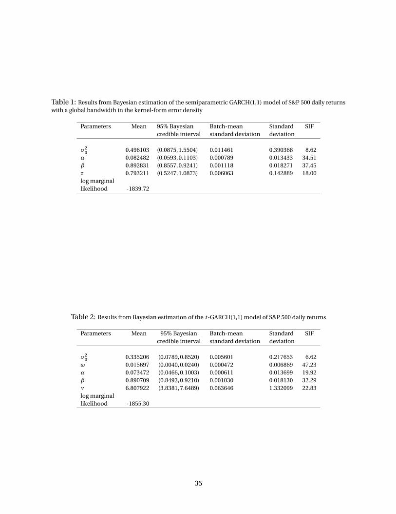
Table 1: Results from Bayesian estimation of the semiparametric GARCH(1,1) model of S&P 500 daily returnswith a global bandwidth in the kernel-form error density

Parameters Mean 95% Bayesian Batch-mean Standard SIFcredible interval standard deviation deviation

σ20 0.496103 (0.0875,1.5504) 0.011461 0.390368 8.62

α 0.082482 (0.0593,0.1103) 0.000789 0.013433 34.51β 0.892831 (0.8557,0.9241) 0.001118 0.018271 37.45τ 0.793211 (0.5247,1.0873) 0.006063 0.142889 18.00log marginallikelihood -1839.72

Table 2: Results from Bayesian estimation of the t-GARCH(1,1) model of S&P 500 daily returns

Parameters Mean 95% Bayesian Batch-mean Standard SIFcredible interval standard deviation deviation

σ20 0.335206 (0.0789,0.8520) 0.005601 0.217653 6.62

ω 0.015697 (0.0040,0.0240) 0.000472 0.006869 47.23α 0.073472 (0.0466,0.1003) 0.000611 0.013699 19.92β 0.890709 (0.8492,0.9210) 0.001030 0.018130 32.29ν 6.807922 (3.8381,7.6489) 0.063646 1.332099 22.83log marginallikelihood -1855.30

35

Table 3: Results from Bayesian estimation of the semiparametric GARCH(1,1) model with a global bandwidth,and the t-GARCH(1,1) model. The corresponding SIF values are given in parentheses, and LML represents thelog marginal likelihood.

Model Parameter Nasdaq NYSE DJIA FTSE DAX AORD Nikkei

Semiparametric σ20 0.737396 0.675171 0.452820 0.672453 0.757102 1.021040 0.841057

GARCH (6.47) (6.58) (6.74) (8.32) (6.25) (7.46) (6.23)α 0.098014 0.086032 0.094623 0.108520 0.144759 0.137622 0.137127

(39.12) (27.55) (19.23) (10.34) (9.78) (23.85) (11.23)β 0.887498 0.892873 0.883619 0.880093 0.854487 0.851735 0.844828

(40.67) (32.08) (19.87) (13.93) (10.36) (26.87) (11.91)τ 0.977918 1.017463 1.241229 1.360150 1.082082 1.228259 1.050393

(9.46) (16.46) (17.48) (8.92) (16.76) (11.91) (8.61)VaR 2.3327 2.1847 1.8587 2.0247 2.2087 1.9937 2.0937LML -1959.64 -1924.85 -1748.03 -1880.29 -1955.95 -1791.04 -2013.62

t-GARCH σ20 0.672198 0.471396 0.312151 0.576110 0.638668 0.946476 0.816669

(4.74) (6.30) (8.94) (5.85) (4.40) (10.32) (6.35)ω 0.024144 0.021031 0.011339 0.030545 0.028463 0.031719 0.064810

(54.95) (31.45) (53.04) (46.68) (59.09) (62.35) (65.09)α 0.071868 0.073784 0.074238 0.084517 0.067160 0.097714 0.112387

(16.63) (10.85) (21.70) (17.91) (21.33) (22.90) (21.14)β 0.892783 0.891033 0.891644 0.875496 0.895703 0.860881 0.837827

(34.41) (24.56) (27.63) (35.07) (38.11) (48.65) (52.06)ν 7.619080 7.530589 6.697563 9.158895 8.110169 10.632002 9.962462

(13.43) (21.14) (23.05) (14.57) (20.86) (10.91) (10.28)VaR 2.0407 1.8027 1.5467 1.8387 1.9207 1.7917 1.9037LML -1973.36 -1936.98 -1750.14 -1874.35 -1950.56 -1788.66 -2023.34

Table 4: Results from Bayesian estimation of the semiparametric GARCH(1,1) model with localized bandwidths,and the corresponding SIF values are given in parentheses. LML represents the log marginal likelihood.

Parameter S&P 500 Nasdaq NYSE DJIA FTSE DAX AORD Nikkeiσ2

0 0.427865 0.751002 0.623526 0.383134 0.680188 0.761025 1.005982 0.838286(6.20) (3.81) (6.44) (4.92) (7.40) (9.15) (8.06) (8.28)

α 0.093154 0.095775 0.094024 0.108472 0.104737 0.098777 0.119007 0.145997(14.60) (14.63) (13.95) (10.61) (8.19) (42.14) (15.11) (13.72)

β 0.893324 0.891723 0.891525 0.879487 0.881261 0.891679 0.866824 0.836636(15.47) (17.07) (16.13) (13.43) (8.80) (23.14) (17.35) (15.99)

τ 0.763784 0.809399 0.746952 0.807333 0.836401 0.842342 0.779654 0.738866(12.19) (13.15) (13.71) (12.77) (22.95) (27.36) (23.98) (20.18)

τε 0.635660 0.417427 0.654049 0.761657 0.528280 0.687812 0.530457 0.427624(28.08) (14.89) (18.41) (24.20) (23.53) (29.69) (25.97) (21.58)

VaR 1.9778 2.3147 2.1587 1.8097 1.9687 2.1207 1.9217 2.0717LML -1835.67 -1958.63 -1918.19 -1733.59 -1876.13 -1949.46 -1787.70 -2012.25

36

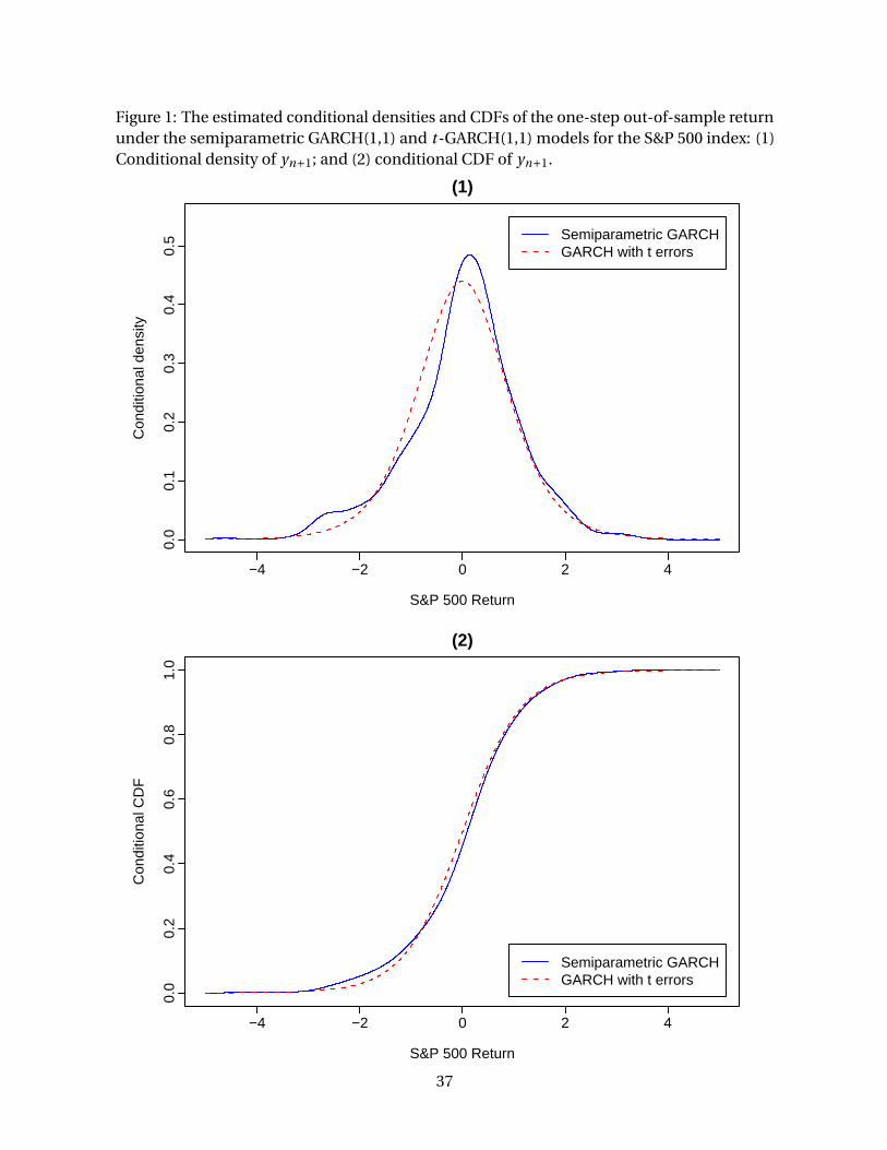
Figure 1: The estimated conditional densities and CDFs of the one-step out-of-sample returnunder the semiparametric GARCH(1,1) and t-GARCH(1,1) models for the S&P 500 index: (1)Conditional density of yn+1; and (2) conditional CDF of yn+1.

−4 −2 0 2 4

0.0

0.1

0.2

0.3

0.4

0.5

(1)

S&P 500 Return

Con

ditio

nal d

ensi

ty

Semiparametric GARCHGARCH with t errors

−4 −2 0 2 4

0.0

0.2

0.4

0.6

0.8

1.0

(2)

S&P 500 Return

Con

ditio

nal C

DF

Semiparametric GARCHGARCH with t errors

37

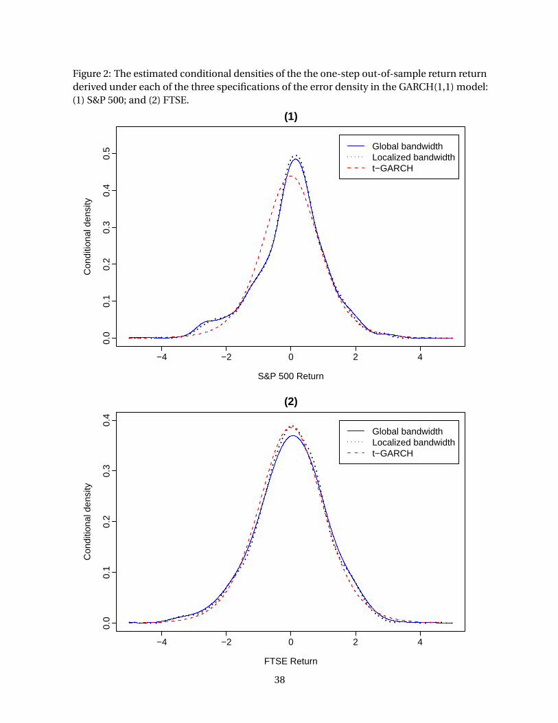
Figure 2: The estimated conditional densities of the the one-step out-of-sample return returnderived under each of the three specifications of the error density in the GARCH(1,1) model:(1) S&P 500; and (2) FTSE.

−4 −2 0 2 4

0.0

0.1

0.2

0.3

0.4

0.5

(1)

S&P 500 Return

Con

ditio

nal d

ensi

ty

Global bandwidthLocalized bandwidtht−GARCH

−4 −2 0 2 4

0.0

0.1

0.2

0.3

0.4

(2)

FTSE Return

Con

ditio

nal d

ensi

ty

Global bandwidthLocalized bandwidtht−GARCH

38