Embed Size (px)
Citation preview
BENDING AND FORCE RECOVERY IN POLYMER FILMS AND MICROGEL
FORMATION
A Thesis
Submitted to the Graduate Faculty
of the
North Dakota State University
of Agriculture and Applied Science
By
Theresa Marie Elder
In Partial Fulfillment of the Requirements
for the Degree of
MASTER OF SCIENCE
Major Program:
Materials and Nanotechnology
August 2017
Fargo, North Dakota

North Dakota State University
Graduate School
Title
BENDING AND FORCE RECOVERY IN POLYMER FILMS AND
MICROGEL FORMATION
By
Theresa Marie Elder
The Supervisory Committee certifies that this disquisition complies with North Dakota State
University’s regulations and meets the accepted standards for the degree of
MASTER OF SCIENCE
SUPERVISORY COMMITTEE:
Andrew B. Croll
Chair
Erik Hobbie
Yechun Wang
Approved:
November 14, 2017 Erik Hobbie
Date Department Chair

iii
ABSTRACT
To determine correlation between geometry and material three different model films:
polymethylsiloxane (PDMS), polystyrene (PS), and polycarbonate (PC), were singly bent and
doubly bent (forming D-cones). Bends were chosen as they are fundamental in larger complex
geometries such as origami and crumples. Bending was carried out between two plates taking
force and displacement measurements. Processing of data using moment equations yielded
values for bending moduli for studied films that were close to accepted values. Force recovery
showed logarithmic trends for PDMS and stretched exponential trends for PS and PC. In a
separate experiment a triblock copolymer of polystyrene–polyacrylic acid–polystyrene was
subjected to different good and bad solvent mixing with any resulting particle morphology
examined. Particles formed more uniformly with high water concentration, particles formed with
high toluene concentration and agitation yielded three separate morphologies.
iv
ACKNOWLEDGEMENTS
This research was made possible by the NDSU Materials and Nanotechnology Graduate
School and the Air Force Office of Scientific Research of the United States. My group including
Dr. Andrew Croll, Timothy Twohig, Dr. Damith Rozairo, Dr. Nasibeh Hosseini, and previous
members including Dr. Bekele Gurmessa also made this research possible and provided
invaluable consultation. Acknowledgement also goes to summer high school students, especially
Alex Rice. Characterization methods: NDSU Electron Microscopy lab for use of SEM
microscopy with Scott Payne, R1 research lab for use of pull tester and AFM, and Veterinary
Diagnostic lab for DIC imaging.
v
DEDICATION
I dedicate this work to all those who were close to and tolerated me prior to and for the duration
of this project and thesis: my parents, my family, my friends, my colleagues, and my adorable
cats. I dedicate this work to those who have supported me in one way or another over the course
of this journey. Among my family that I dedicate this to are my parents, Bessie and Tony, and
their spouses Corey Elletson and Chantal Elder respectively, my brother Craig Elder and his wife
Megan, my sisters by marriage and in spirit Cassandra Lucero and Ginette Castaneda and their
families, my uncle Tim Carr, and my grandparents, Richard and Beverly Elder, Rosalyn and
Deke, Grandma Renee, Harry and Lucy Moss, and Karen Elletson. I also dedicate this work to
my wonderful pets, my cats Morgan and Prince, as well as those past, yet to come, and those of
friends, family members, and strangers that I have bonded with. I also dedicate this to all of my
wonderful friends many of which are like family to me, including Lydia Kelley, her mother
Lodema, and the Kelley family, Karen Ufert and her family, Soodabeh Einharjar, Sharonda
Fudge, Marie Davis, Nicole Jean, Erica Gee, Jo Nikole, Linda Berry, Kenya Kraft, Cassy, Jah
Son, Sita Prakash, Terrance, Kami, and numerous others whom time and space does not allow
me to explicitly name, but that I treasure and include in this list. I would also like to thank all of
my professors and teachers, both undergraduate and graduate, for their tutelage, especially: Dr.
Andrew Croll, my research mentor, who accepted me into his group and guided me along the
way, my committee members Dr. Erik Hobbie and Dr. Yechun Wang, and Dr. Ryan Winburn,
my undergraduate research mentor. My colleagues and fellow graduate students also deserve to
be listed in this dedication for their consultations and social presence: Timothy Twohig, Dr.
Nasibeh Hosseini, Dr. Damith Rozairo, Jamie Froberg, Sam Brown, and everyone else that I
encountered during the time of my studies that assisted me in some way.
vi
TABLE OF CONTENTS
ABSTRACT ................................................................................................................................... iii
ACKNOWLEDGEMENTS ........................................................................................................... iv
DEDICATION ................................................................................................................................ v
LIST OF FIGURES ..................................................................................................................... viii
LIST OF ABBREVIATIONS ....................................................................................................... xii
LIST OF SYMBOLS ................................................................................................................... xiv
INTRODUCTION .......................................................................................................................... 1
Polymers ...................................................................................................................................... 1
CHAPTER 1. STATIC AND DYNAMIC SINGLE BENDS OF POLYMER FILMS ................. 8
Background ................................................................................................................................. 8
Theory ....................................................................................................................................... 13
Experiment ................................................................................................................................ 15
Sample Film Preparation ....................................................................................................... 15
Mechanical Testing ............................................................................................................... 16
Apparatus ............................................................................................................................... 17
Analysis Tracker .................................................................................................................... 18
Tensile Test on PDMS........................................................................................................... 19
Results and Discussion .............................................................................................................. 19
Conclusion ................................................................................................................................. 30
CHAPTER 2. BENDING AND FORCE RECOVERY OF D-CONE IN POLYMER
FILMS ........................................................................................................................................... 32
Background ............................................................................................................................... 32
Theory ....................................................................................................................................... 33
Experiment ................................................................................................................................ 34

vii
Results and Discussion .............................................................................................................. 35
Conclusion ................................................................................................................................. 45
CHAPTER 3. MICROGEL PARTICLES FROM TRIBLOCK COPOLYMERS PS-PAA-
PS .................................................................................................................................................. 47
Background ............................................................................................................................... 47
Theory ....................................................................................................................................... 55
Experiment ................................................................................................................................ 57
Polymer Solutions ................................................................................................................. 57
Microscopy Preparations ....................................................................................................... 57
Results and Discussion .............................................................................................................. 59
Water Crashing ...................................................................................................................... 61
Toluene Crashing................................................................................................................... 69
Conclusion ................................................................................................................................. 74
REFERENCES ............................................................................................................................. 75

viii
LIST OF FIGURES
Figure Page
1. A general schematic curve of stress-strain mechanics in amorphous polymeric
solids ................................................................................................................................... 6
2. The single bend geometry and dimensional measurements taken of a sample film ......... 17
3. Large scale apparatus for two plate bending used in this work ........................................ 18
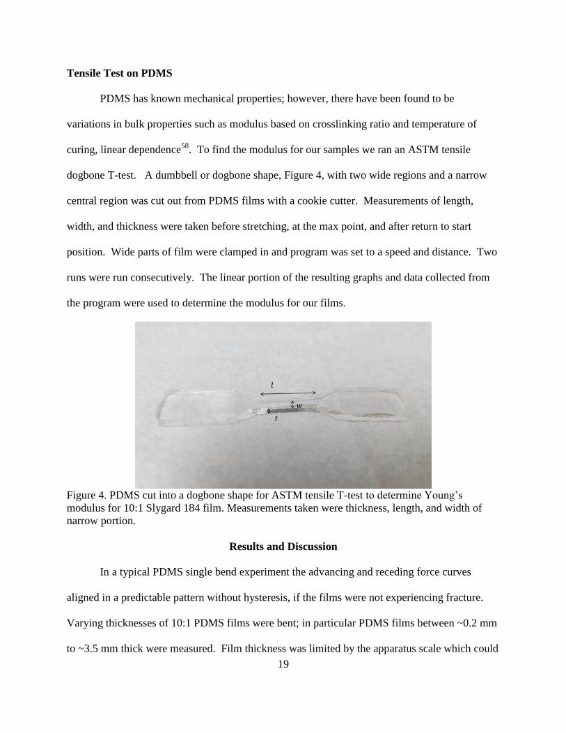
4. PDMS cut into a dogbone shape for ASTM tensile T-test to determine Young’s
modulus for 10:1 Slygard 184 film ................................................................................... 19
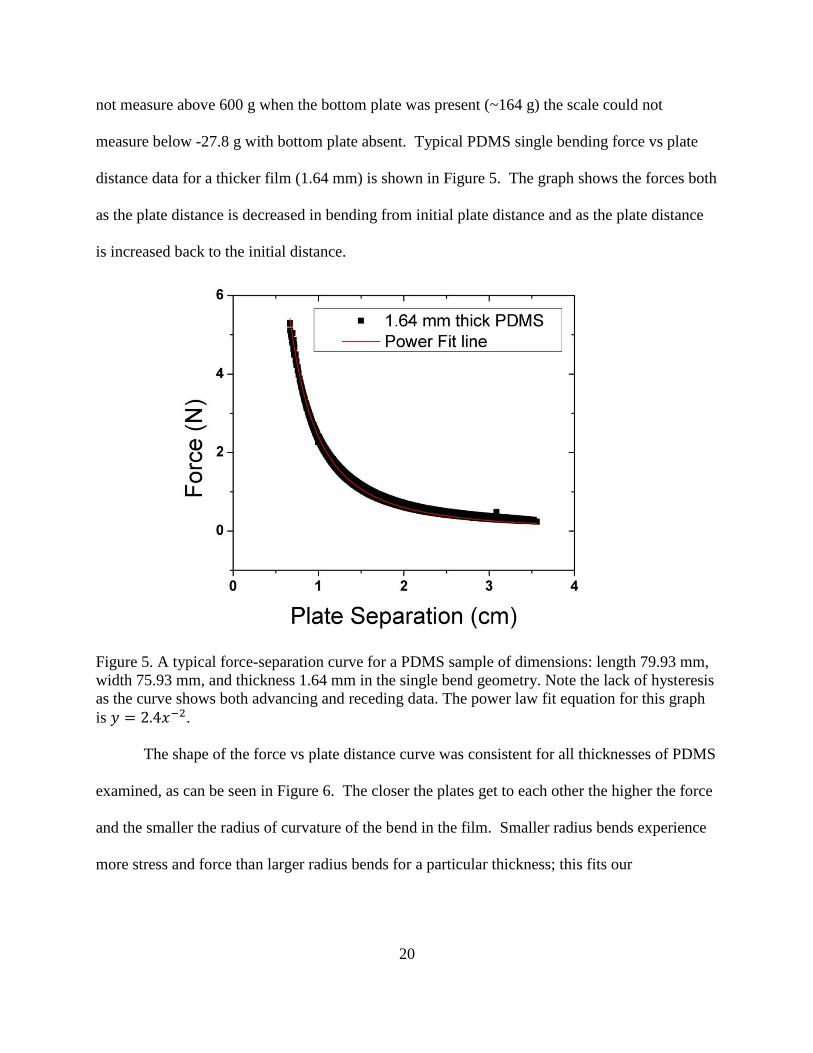
5. A typical force-separation curve for a PDMS sample of dimensions: length 79.93
mm, width 75.93 mm, and thickness 1.64 mm in the single bend geometry .................... 20
6. PDMS single bend compilation graph of films of thicknesses ≥ 0.23 mm ....................... 21
7. A force-separation curve for a PS sample of dimensions: length 39.88 mm, width
15.02 mm, and thickness 25.55 μm, in the single bend geometry .................................... 22
8. PS single bend compilation graph……………..………………………………………...23
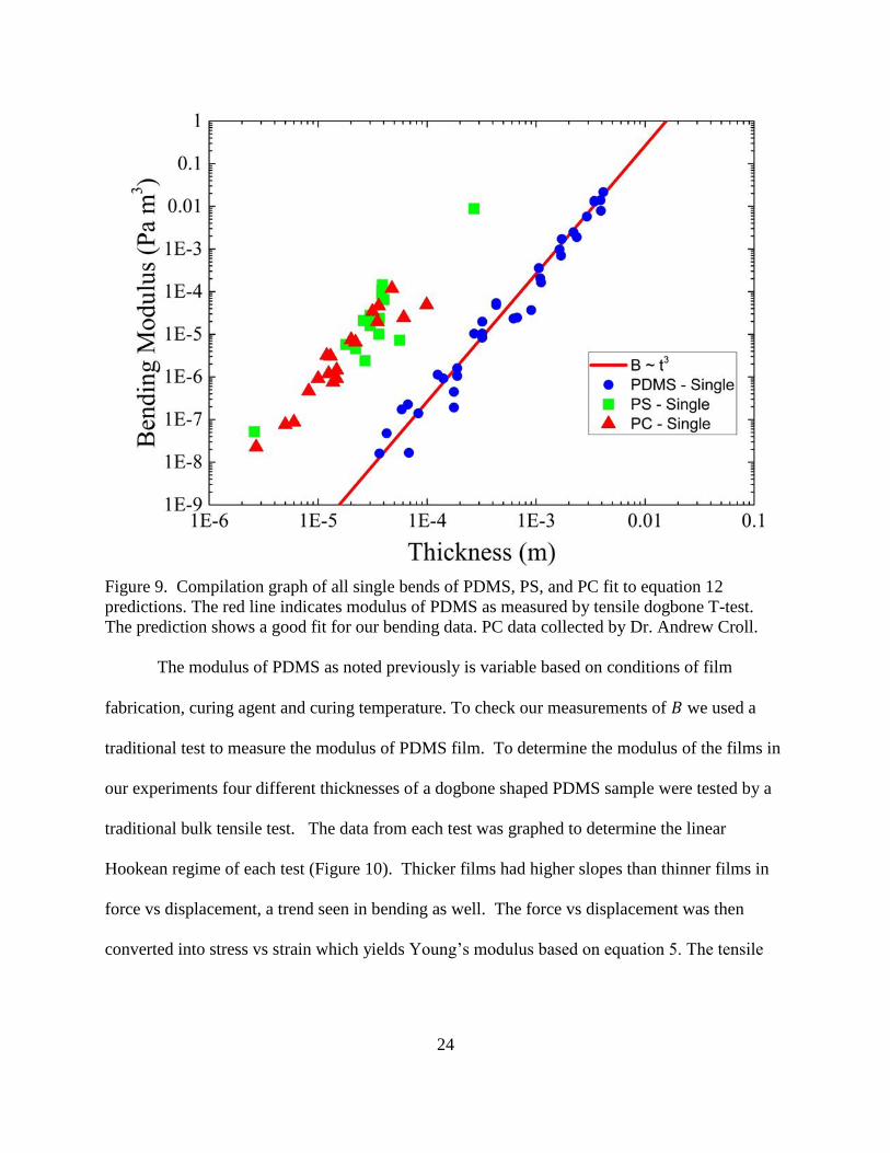
9. Compilation graph of all single bends of PDMS, PS, and PC fit to equation 12
predictions ......................................................................................................................... 24
10. Linear regimes of dogbone tensile T-tests for four different thicknesses of 10:1
PDMS.. .............................................................................................................................. 25
11. PDMS single bend force-time graph for a 1.06 mm thick film ........................................ 26
12. All samples of PDMS force recovery for single bends. .................................................... 27
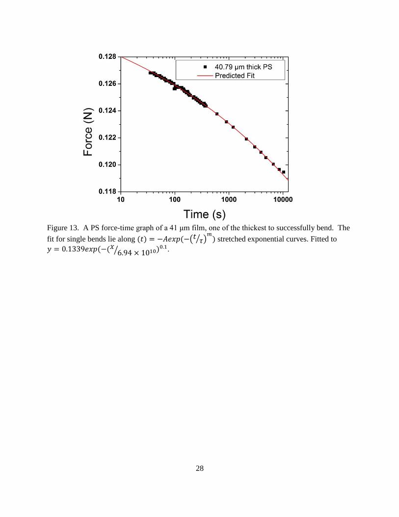
13. A PS force-time graph of a 41 μm film, one of the thickest to successfully bend............ 28
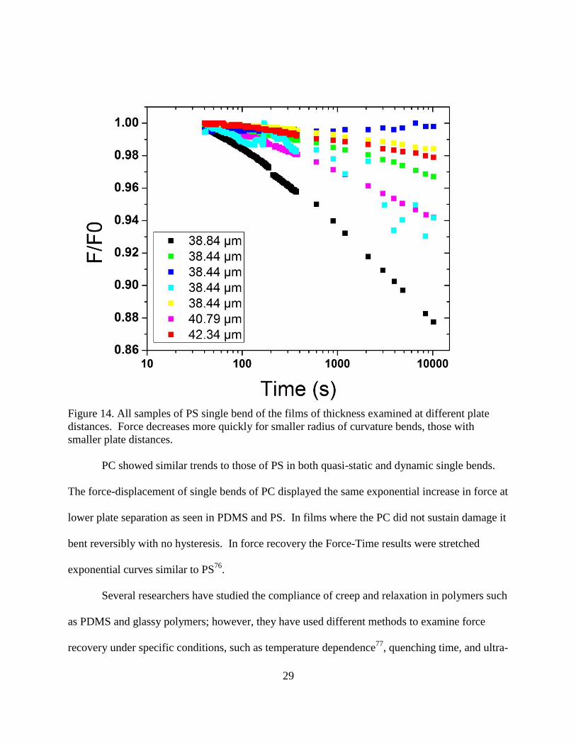
14. All samples of PS single bend of the films of thickness examined at different plate
distances.. .......................................................................................................................... 29
15. A doubly bent film of 0.67 mm thick PDMS between two plates with D-cone
formed. .............................................................................................................................. 34
16. A typical force-separation curve for a doubly bent 10:1 PDMS sample of
dimensions: length 79.62 mm, width 73.05 mm, and thickness 0.67 mm in the
single bend geometry ........................................................................................................ 36
17. PDMS double bend compilation graph of films ≥ 0.23 mm thickness. Force has
been normalized ................................................................................................................ 37
ix
18. A force-separation curve for a doubly bent PS sample of dimensions: length 43.5
mm, width 20.54 mm, and thickness 33.10 μm ................................................................ 38
19. Three consecutive bends of a PS film to decreased plate separation. PS film was
of dimensions: length 43.5 mm, width 20.54 mm, and thickness 33.10 μm in
double bend geometry.. ..................................................................................................... 39
20. Bending modulus-thickness plot of all double and single film bends on log-log
plot. ................................................................................................................................... 40
21. PDMS force-time graph for a 1.72 mm thick film doubly bent with pre-double
bend dimensions of 80.15 mm length and 75.77 mm width. ............................................ 41
22. A PS force vs. time graph of a 33.10 μm film with pre-bend length of 43.5 mm
and width of 20.54 mm ..................................................................................................... 42
23. All samples of PDMS force recovery for single and double bends, normalized .............. 43
24. All samples of PS single bend of the films ~40 μm thickness at different plate
distances. Force decreases more quickly for smaller radius bends. ................................. 44
25. A general schematic of particle swelling. Before indicates a particle in an
unswelled state and after indicates a solvent swollen particle .......................................... 49
26. Representation of particle made from a triblock copolymer in which a network is
formed from end group aggregation ................................................................................. 54
27. Master solution of PS-PAA-PS 1:50:1 ratio with added dye dried on Si wafer and
rehydrated with a drop of distilled H2O. ........................................................................... 60
28. Elastomer bubbles ar 50x magnification on optical microscope a) and b) PS-PAA-
PS 1:50:1 triblock master solution with dye in a water crashed sample, multiple
elastomer bubbles formed. c) and d) elastomer bubble formation in glycerol of
PS-PAA-PS 1:20:1 triblock master solution without dye. ................................................ 60
29. Different MS:water ratios of PS-PAA-PS 1:50:1 triblock at 50x magnification on
optical microscope ............................................................................................................ 61
30. PS-PAA-PS 1:50:1 triblock a), b), c) 1:10 ratio water crashing and heat assisted
solvent evaporation at 50x magnification. d) sample dried in center of washer at
5x magnification e) and f) at 50x magnification. .............................................................. 62
31. PS-PAA-PS 1:50:1 with dye at 1:4 ratio MS: water dried and rehydrated a), b), c)
are at 5x magnification d), e), and f) are at 50x magnification ......................................... 63
32. AFM imaging of 1:4 water crashed PS(1000)-PAA(50000)-PS(1000) master
solution with dye a) 20000 nm x 20000 nm image with height range ~35-80 nm b)
2000 nm x 2000 nm with 67.6 nm height ......................................................................... 64
x
33. PS-PAA-PS 1:20:1 ratio at 1:4 water crashing after rehydration a) and b) are at 5x
magnification c), d), e), f) are at 50x magnification from different areas of a) and
b) and surroundings on the substrate ................................................................................ 65
34. AMF micrograph of 1:20:1 PS-PAA-PS water crashed at 1:4 ratio. ................................ 65
35. SEM images of water crashed PS-PAA-PS 1:20:1. 1:4 MS: water (left) 1:9 MS:
water (right).. .................................................................................................................... 66
36. PS-PAA-PS 1:20:1 in a 1:4 water crashing at 5x magnification, the first 5 from
one day and the last from a different day. ......................................................................... 66
37. PS-PAA-PS 1:20:1 in 1:4 water crashing taken on 4 different days from 4
different samples at 50x magnification ............................................................................. 67
38. Confocal imaging of PS-PAA-PS 1:50:1 crashed water in 1:4 ratio rehydrated at
10x magnification ............................................................................................................. 68
39. Confocal imaging at 50x of PS-PAA-PS 1:50:1 ratio crashing in water 1:4 and
rehydrated, viewed at 50x with dyed particles visible under fluorescence channel
on the right ........................................................................................................................ 68
40. Particles visible in solution and on glass from PS-PAA-PS 1:20:1 ratio in water
viewed on Zeiss microscope LSM-T-PMT Define focus with HAL 100
attachment Zen 2011 software.. ........................................................................................ 69
41. PS-PAA-PS 1:50:1 added dropwise to ~20mL of toluene at 50x magnification. ............ 70
42. PS-PAA-PS 1:50:1 added dropwise to ~20mL of toluene at 50x magnification
concentrated a) dried with heater b) through f) were dried in air ..................................... 70
43. PS-PAA-PA 1:50:1 mixed in excess toluene for 24 hours allowed to dry in air and
rehydrated.. ....................................................................................................................... 70
44. PS-PAA-PA 1:50:1 mixed in excess toluene for 24 hours rehydrated and dried at
70 °C on a hot plate a) 5x magnification b) through i) 50x magnification.. ..................... 71
45. PS-PAA-PS 1:50:1 mixed in toluene and heat dried. AFM image scan size 10000
nm x 10000 nm of height range ~20-50 nm ..................................................................... 72
46. PS-PAA-PS 1:20:1 mixed in toluene for 24 hours at 5x magnification ........................... 72
47. PS-PAA-PS 1:20:1 mixed in toluene for 24 hours 3 different patterns a) discrete
particles, b) and c) lizard skin d) through l) haloed particles............................................ 73
48. PS-PAA-PS 1:20:1 passed through excess toluene in seperatory funnel at 50x
magnification .................................................................................................................... 74

xi
49. PS-PAA-PS 1:50:1 passed through excess toluene in seperatory funnel at 50x
magnification .................................................................................................................... 74

xii
LIST OF ABBREVIATIONS
DNA ...............................................................Deoxyribonucleic acid.
1D ...................................................................One dimensional.
2D ...................................................................Two dimensional.
3D ...................................................................Three dimensional.
PS ...................................................................Polystyrene.
PC ...................................................................Polycarbonate.
PDMS .............................................................Polydimethylsiloxane.
MPa ................................................................Mega Pascal.
GPA................................................................Giga Pascal.
g......................................................................gram(s).
s ......................................................................second(s).
mm .................................................................millimeter(s).
cm ...................................................................centimeter(s).
μm ..................................................................micrometer(s).
ASTM ............................................................American Society for Testing and Materials.
D-cone ............................................................Developable cone.
min .................................................................minute(s).
°C ...................................................................Degrees Celsius.
pH ...................................................................Potential of Hydrogen.
DVB ...............................................................Divinylbenzene.
PNIPAM ........................................................Poly(N-isopropylacrylamide).
PAA................................................................Polyacrylic acid.
PS-b-PAA ......................................................Polystyrene-block-poly(acrylic acid).
Mn ..................................................................Number average molecular weight.
xiii
PDI .................................................................Polydispersity index.
THF ................................................................Tetrahydrofuran.
DMF ...............................................................N,N-Dimethylformamide.
MΩ .................................................................megohm(s).
mL ..................................................................milliliter(s).
AFM ...............................................................Atomic Force Microscope.
MS ..................................................................Master Solution.
SEM ...............................................................Scanning Electron Microscope.
Si ....................................................................Silicon.
DIC .................................................................Differential Interference Contrast.
xiv
LIST OF SYMBOLS
𝑇𝑔 ....................................................................Glass transition temperature,
𝑇𝑚 ...................................................................Melting temperature.
𝜀(𝑡) .................................................................Strain as a function of time.
𝜎0 ....................................................................Initial stress.
𝐽(𝑡) .................................................................Material compliance as a function of time.
𝜎(𝑡) ................................................................Stress as a function of time.
𝜀0 ....................................................................Initial strain.
𝐺(𝑡) ................................................................Material stiffness as a function of time.
𝜎 .....................................................................Stress.
𝐹 .....................................................................Force.
𝐴 .....................................................................Area.
𝜀𝑖𝑘 ...................................................................Strain along the i and k axes.
𝑥𝑘 ...................................................................Coordinate axis of displacements in k.
𝑥𝑖 ....................................................................Coordinate axis of displacements in i.
𝑢𝑘 ...................................................................Displacement along k axis.
𝑢𝑖 ....................................................................Displacement along i axis.
𝜀 ......................................................................Strain.
𝐸 .....................................................................Young’s modulus.
𝜈 .....................................................................Poisson’s ratio.
𝜎𝑥𝑥 ..................................................................Stress in x direction.
𝜀𝑥𝑥 ..................................................................Strain in x direction.
𝜀𝑦𝑦 ..................................................................Strain in y direction.
𝜀𝑧𝑧 ...................................................................Strain in z direction.
xv
𝑀𝑡𝑜𝑡 ................................................................Total moment.
𝜀𝑡 ....................................................................Strain in transverse direction.
𝜀𝑙.....................................................................Strain in longitudinal direction.
𝑅 .....................................................................Radius of curvature.
𝐼𝑥 ....................................................................Cross sectional area.
𝑡 ......................................................................Thickness.
𝑏 .....................................................................Width.
𝐵 .....................................................................A parameter in moment equation that includes the
thickness.
𝑈𝑠 ...................................................................Stretching energy.
𝐸𝑠 ....................................................................Stretching stiffness.
𝛾 .....................................................................In plane strain.
𝛥𝑆 ...................................................................Area of stretched region.
𝑈𝑏 ...................................................................Bending energy.
𝐸𝑏 ...................................................................Bending modulus.
𝜅 .....................................................................Mean curvature in D-cone core.
𝑅𝑐 ...................................................................Radius of D-cone.
𝛷 ....................................................................Angle of D-cone formed.
𝑅𝑠 ...................................................................A measurement of the sheet.
𝛷2 ...................................................................Flory particle swelling.
𝑋 .....................................................................Cross-links within a volume of collapsed particle.
𝑉𝑐 ....................................................................Volume in a collapsed particle.
𝑋12 ..................................................................Flory solvent-polymer interaction parameter.
1
INTRODUCTION
Polymers
Polymers are a type of soft condensed matter with growing importance in our daily lives1.
Polymers, natural and synthetic, are in use in technology, buildings, paints, vehicles, medical
devices2, clothing, and food. Natural polymers include silk, cotton, cellulose
3, DNA, proteins,
and polysaccharides1. Synthetic polymers include polystyrene, polyethylene, Kevlar,
polycarbonate, nylon, and siloxanes. Solids made from polymers can have a multitude of
dimensions as they can be molded into shapes, fibers, and thick coatings using a variety of
methods including: injection molding, thermoforming, blow molding, sintering, and extrusion3.
Understanding these polymers and how they react to strain and other processes is useful as they
continue to infiltrate all aspects of daily life.
A polymer is a macromolecule composed of repeating units of smaller molecules called
monomers. Monomers are covalently or physically bonded together forming a chain which can
be variable in length, composition, and architecture. Monomers that can be polymerized
generally fall into one of three categories: those containing double or triple bonds, those having
functional end groups, or cyclic molecules. Double and triple bonds can break to form two new
bonds to other molecules and perpetuate polymer growth. Cyclic molecules are similar in that a
bond can break between two elements in a ring, incorporating a growing polymer or other
monomers. Monomers that have functional end groups can react with the functional end groups
of other monomers to bond together and perpetuate the chains. A polymer comprised of only
one type of monomer is a homopolymer. A polymer comprised of more than one monomer is
known as a copolymer. Polymers come in a number of different architectures based on monomer
and initiator reactivity including: chain, branched, grafted, star, and crosslinked3,4
.
2
Copolymers are differentiated by their monomer arrangements in relation to each other.
If the unlike monomers alternate uniformly one after another the polymer is known as an
alternating copolymer. Random copolymers are those where the arrangement of monomers are
randomly dispersed throughout the polymer with no specific pattern. If two lengths of different
homopolymer are bound together the resulting polymer is referred to as a block copolymer. An
amphiphilic copolymer can be created when a block of homopolymer that is hydrophobic
connects to a block of homopolymer that is hydrophilic4. Amphiphilic polymers have a
tendency to minimize contact in poor solvents, aggregating with other polymer and molecules in
order to minimize surface area that can interact with the poor solvent1,2,3
.
The versatility of polymeric materials arises from their unique physical and chemical
properties attributable to their large length scales and high molecular weights. The large number
of atoms in a polymer exponentially increases weak intermolecular forces: van der Waals, H-
bonding, ionic forces, and dispersion forces; rather than chemical forces and potentials that
dominate individual and small molecule interactions4. These forces can lead to polymer
entanglement with themselves and other polymers, complex arrangements similar to tangled
cords which restrict individual polymer movements. The restriction of motion is often depicted
as a tube at any given time; the polymer is confined to moving only within the tube as the
surrounding polymer and weak forces limit the space it can occupy at that given time. With
enough time the polymer might reptate out of its particular tube or the tube might change
dimensions as the entire system is in motion, rearranging while in solution or above the
polymer’s glass transition temperature (𝑇𝑔)1.
Polymer melts are considered “fragile liquids” with significant increases in viscosity as
the temperature of the system decreases5. Melts are polymer systems above a certain
3
temperature, the melt temperature, 𝑇𝑚6. The behavior of homopolymer melts resembles that of
ideal gases as intermolecular and intramolecular forces dominate over fluctuations in density8 at
any given point in the system. This assumed ideal of identical interactions between ideal chains
approximate experimental behaviors in bulk accurately9. Melts with less volume might deviate
from ideal behavior8. In fluid polymer systems, melts and solutions, there is freedom of
movement for monomers around their bonds; therefore, the polymers assume different
conformational states such as helices and coils7.
Polymer solutions are polymer systems in solvents that do not exhibit melt behavior, the
solvent affects monomer interactions either through increasing or decreasing contact with
neighboring monomers. Polymers in solution exhibit excluded volume effects where a neighbor
monomer cannot occupy a certain area of space due to it being occupied by another monomer or
solvent molecules7. Monomers might have frictional interactions with neighboring monomers
when in good solvents10
. In good solvents the monomers are also surrounded by shells of
solvent molecules that expand the chain away from other monomers and increase the overall area
occupied by the polymer chains. These are called expanded chains7. Polymers in bad solvents
will experience aggregation as solvent molecules and monomer prefer contact with themselves
and try to reduce surface contact with each other1,7
.
Polymer chains can link together in numerous places to form macroscopic molecules.
The bonding of neighbor chains through covalent bonds, reversible physical bonding such as
entanglements or through linker molecules is known as crosslinking1. Crosslinking greatly
changes the properties of the material by increasing molecular weight, increasing thermal
stability, and changing stress-strain dynamics. As neighboring polymers crosslink together
forming a network the macromolecule grows, increasing in molecular weight and reducing
4
solubility. Thermal stability is increased due to a higher number of bonds that would need to
break in order to separate molecules leading to a built in redundancy that improves mechanical
properties. For physically crosslinked polymers the material might have the beneficial
possibility of self-healing through the reforming of bonds under the right conditions11
.
The density of crosslinking distinguishes if the resulting macromolecule is a gel,
elastomer, or resin. Gels are loosely crosslinked and can absorb solvents readily resulting in
swelling. Elastomers vary in crosslink density and show varied response to stress and stretching
based on the degree of crosslinking. Gum is a natural elastomer of cellulose micro fibrils1 which
have fewer cross-link bonds than a commercial rubber elastomer which imparts greater
stretching and self-healing properties but higher malleability under stress loads. Many
commercial elastomers are more highly crosslinked resulting in a more fixed shape and lower
mobility under stress with higher recovery of the original dimensions after the stress stimulus is
removed2. The often desirable reversible reaction to stress (elastic stretching) can be as large as
500% and 1000% of initial length due to a low modulus that increases as strain increases.
Elastomer strength can be increased through the addition of reinforcing inorganic fillers, large
quantities of nano-sized particles that do not participate in cross-linking12
, make a filled
elastomer. The most highly crosslinked macromolecules are resins which are similar to typical
hard solids in their hardness, resiliency to heat3, and high tensile strength
13. Unlike other less
crosslinked polymer networks, resins do not easily absorb solvent3 and are resilient to
chemicals14
.
Some polymers have been shown to crystallize at low temperatures, below Tm, exhibiting
both crystalline hierarchical ordered structures and interspersed amorphous regions. The
amorphous regions result from irregularities and defects of packing as polymers crystallize
5
through folding sections of their chains into folded-chain lamella structures. The folding must
occur around entanglements with themselves and neighbor polymers; kinetics more than
thermodynamic equilibriums determine the resulting crystalline morphology1. Methods of
crystallization that maintain temperatures close to melting point or melt temperatures for
extended periods of time result in more highly ordered crystallization than those where
quenching halts polymer folding prematurely. The degree of crystallinity imparted also depends
on the polymer composition as monomers that are less bulky or have larger attractive forces
guiding them into crystallization will crystallize more readily than those lacking either
condition3.
Glasses are amorphous like liquids, lacking long range order at high temperatures even if
they appear to have order at small scales. Bulky groups keep glassy polymers from uniformity by
acting as nucleating clusters15
that expand, these clusters fit into irregular mosaic arrangements5
rather than ordered arrangement. Glass formation can also be related to voids between
monomers being occupied by solvents, or other molecules5 which alters polymer motion. The
transition into a glass from a solution or melt is characterized by a temperature, 𝑇𝑔 the
temperature at which the system has a low kinetic energy and begins to solidify1,16
. 𝑇𝑔 can be
thickness dependent with thinner polymer systems having a lower or higher 𝑇𝑔 due to increased
heat diffusion and higher surface area to volume ratios than polymer in bulk17
. Substrate effects
can also lower or raise 𝑇𝑔 from attractive or repulsive forces that alter mobility18
.
The effect entanglement has on polymer solution and melt mechanical properties are
increased viscoelasticity, resistance to shear forces1, and non-Newtonian viscosity. At low
density of entanglement the viscosity is high while at high density the behavior is elastic19
. In
solutions of good solvent certain polymers show rod-like behavior of monomers15
. Polymer
6
systems show non-Newtonian variable viscosity under shear due to chain stretching and
entanglements which lead to shear-thinning or shear-thickening rheological behavior20
. Fracture
appearing as macroscopic discontinuity, even in highly dense systems experiencing shear or in
melts are rare19
. For most practical purposes, it is more valuable to know the mechanical
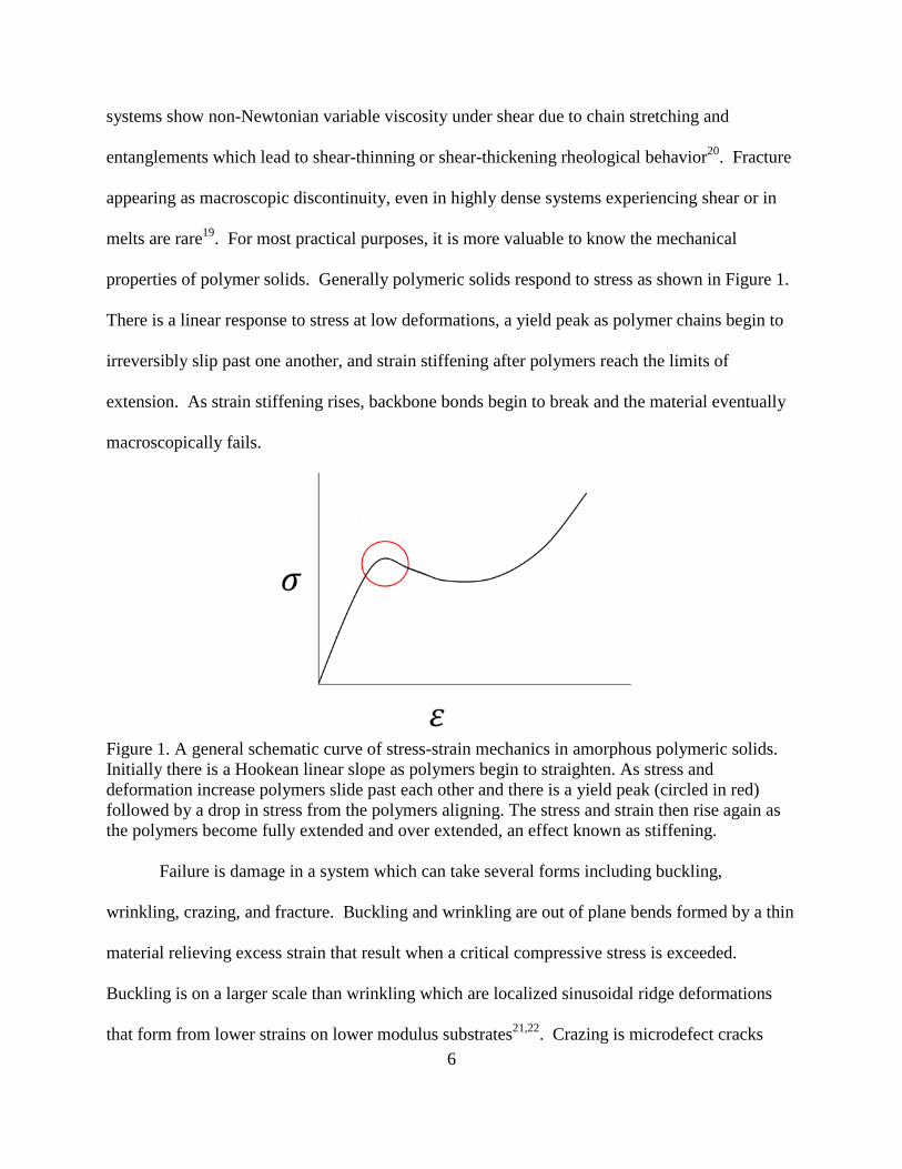
properties of polymer solids. Generally polymeric solids respond to stress as shown in Figure 1.
There is a linear response to stress at low deformations, a yield peak as polymer chains begin to
irreversibly slip past one another, and strain stiffening after polymers reach the limits of
extension. As strain stiffening rises, backbone bonds begin to break and the material eventually
macroscopically fails.
Figure 1. A general schematic curve of stress-strain mechanics in amorphous polymeric solids.
Initially there is a Hookean linear slope as polymers begin to straighten. As stress and
deformation increase polymers slide past each other and there is a yield peak (circled in red)
followed by a drop in stress from the polymers aligning. The stress and strain then rise again as
the polymers become fully extended and over extended, an effect known as stiffening.
Failure is damage in a system which can take several forms including buckling,
wrinkling, crazing, and fracture. Buckling and wrinkling are out of plane bends formed by a thin
material relieving excess strain that result when a critical compressive stress is exceeded.
Buckling is on a larger scale than wrinkling which are localized sinusoidal ridge deformations
that form from lower strains on lower modulus substrates21,22
. Crazing is microdefect cracks
7
whose sides remain connected by polymer fibrils23
. Fracture is cracks propagating in a material
where the two sides are not connected; crazing can progress to fracture when enough stress is
applied to break the connecting fibrils24
.
The broad interesting behavior of polymers resulting from their unique properties and the
range of polymeric materials that can be made inspired our research. In this thesis polymer film
stress response to static and dynamic bending and kinetic microgel assembly will be discussed.
We define static bending as bending with incremental equilibrium points from constant speed
loading and dynamic bending as constant load non equilibrium bending with changing
microscopic arrangement as a result. The thesis is divided into three chapters for clarity. First is
a chapter on static and dynamic single bends, in which we bent 2D sheets of polymeric film in
our experiment. Specifically the film was deformed at constant speeds between two plates to
different maximum displacements. At maximum displacement force recovery over time was
measured. Next, is a chapter on static and dynamic double bends introducing the D-cone
geometry. Finally, the third chapter is on the formation of microgel particles using amphiphilic
block copolymers and a kinetically hindered self-assembly process. Polymeric materials are
widely used so further understanding of their engineering properties in bending, under loads, and
in microgel particles are useful to their applications and engineering.
8
CHAPTER 1. STATIC AND DYNAMIC SINGLE BENDS OF POLYMER FILMS
Background
Thin systems with alterable shape are finding new uses in everyday life such as
stretchable bio-medical electronics25,26
including folding biosensors27,28
, gas sensors, artificial
muscles, bendable memory devices29
and phones30
. The potential for 2D materials that can be
turned into 3D materials can be seen in retractable shapeable solar panels and temporary
residences31
, foldable or flat-laying structures for use in space32,33
, or in situ medical devices34
.
The ability to stretch, twist, and form shapes can give improved mechanical properties, add
functionality, and provide structure dependent attributes35
: adjustable surface areas36
, additional
axes for accuracy in sensors28
, and additional spaces or breaks between regions29
that can serve
many purposes including as fluidic channels27
. Shapeable systems have the added advantage of
cost savings35
as they can be made from paper29
, graphene37
, fabrics31
, and polymeric
materials27,29,34,35,38
. The multitude of advantages and uses of 2D systems makes understanding
their mechanics and force responses useful.
The formation of the thin materials into predetermined geometries can be done in a
number of ways; bending and folding such as origami, cutting, or a combination such as
kirigami. Bending is a global deformation of a system from linear to a curve induced by moving
sections closer together. Folds are localized linear deformations34
of sharper curvature than
bends. Origami is the art of paper folding used to make a shape by stretching and bending a 2D
material out of plane34,37,39,40
. The out of plane bending is often in the form of creases to create
defined shapes and increase complexity34
. Kirigami is similar to origami in that it is a method of
folding out of plane, however, it also employs cutting to form complex shapes or to relieve
9
strain38
. Crumples which are complex networks of folds, ridges, and creases compressively
deform under stress41,42,43, 44, 45
and can be formed through balling up a material.
A large body of research has formed around the formation of certain shapes, complex and
simple, both experimentally and theoretically through origami and kirigami methods. Origami
or kirigami designs can be built into a thin material in various ways: selective molding of thin
and thick regions46
, built in hinges arranged in tessellated patterns of rigid segments47,48,49
, local
modulus variations25,50
, locally induced damage51
, thermal actuation34
, interlocking sections or
sections attracted to each other through forces such as magnetism49
, hydrophilic attractions36
, and
electrical stimuli52
.
During and after the shape changes the system needs to remain functional26
as any
damage can deplete or prevent functionality53
. For a number of applications it is also crucial for
the shape changes to be able to be formed quickly, reliably38
, with reversibility34
, and stability.
The morphology change from one shape to another is a mix of mechanism and structure35
. The
stress-strain response and failure are engineering-relevant properties that are necessary to predict
the overall behavior in a system. Our research focuses on the mechanics of structure in
conjunction with the material properties of the system37
. In particular we examine the origami
relevant structure, a single bend.
Single bends were chosen as they are non-unique structures that can be used individually
or in more complex geometries49
such as origami and crumples. Bends contain compression and
tension29
around a central neutral axis. Bending mechanics are useful in determination of the
maximum stress a system can sustain before failure. Failure can be in the form of fracture53
,
buckling, or crazing. As polymeric materials have the potential to satisfy engineering
10
requirements for shape changing systems at low cost34,38
we chose to use polymer films in our
bending experiments.
A polymer’s mechanical utility is determined primarily from its mechanical properties
such as its stress-strain responses, which may be complex and contain features such as elastic
deformation, flow, and creep3. In order to study how these fundamental material properties
influence origami structure we chose three different model polymer films. The three different
thin polymeric films with varying responses to stress are used to highlight material differences,
polystyrene (PS) and polycarbonate (PC), both glassy materials, and polydimethylsiloxane
(PDMS), a filled elastomer.
PDMS is used commercially in a variety of products including sealants, biomedical
applications, and to create hydrophobic surfaces. It is a hybrid polymer formed from monomers
of Dimethysilanediol, an inorganic-organic, that when mixed with a curing agent initiates
crosslinking to form a rubber analog2. It is considered a flexible filled elastomer and can be
stretched54,55
. Silicones like PDMS are commonly used to surround electronic components due
to their insulation qualities56
. Sylgard 184 PDMS has low hardness with a modulus that
increases with increasing curing agent reaching maximum values at a 9:1 polymer to curing
agent weight ratio. In our bending experiment we used 10:1 PDMS that has bulk tensile or
fracture strength of 2.24 MPa with a Poisson ratio of 0.535, and an elastic modulus of 2.60
MPa56,57
. The exact material properties are also dependent on curing temperature. The bulk
modulus, Young’s modulus, ultimate tensile strength, ultimate compressive strength, and
compressive modulus vary with curing temperatures between 25-200 °C: 2.20-4.95 GPa , 1.32-
2.97 MPa which increases linearly with temperature, 3.51- 7.65 MPa, 51.7-31.4 MPa, 186.9-
117.8 MPa, respectively58
.
11
PS was one of the first polymers synthesized; it is a glassy polymer of styrene monomers
with a 𝑇𝑔 near 100 °C. PS is in common use in many current applications due to the rigidity and
transparency of the polymer when molded. Among the current applications are plastic lenses,
toys, disposable dishes and food containers, and electronics. PS due to the packing qualities of
the phenyl groups along the C backbone is amorphous and brittle with failure resulting in crazing
and cracks2 when yield strength of 28.7-41.4 MPa
59 is surpassed, lower for films below 100 nm
thickness60
. General purpose polystyrene has a Young’s modulus of 3-3.5 GPa , tensile strength
of 30-100 MPa61
, flexural strength of 42.06 MPa, flexural modulus of 3.275 GPa, and
compressive strength of 99.97 MPa62
.
PC is commonly used in water bottles and food containers as well as bullet-resistant
windows. PC like PS is a glassy polymer, composed of two monomers Bisphenol A and
Phosgene that link via condensation polymerization. PC is transparent with a high refractive
index. PC is less brittle than PS with failure tending toward plastic deformation rather than
breakage2. PC has Young’s modulus of 2.0-2.6 GPa, ultimate tensile strength of 52-75 MPa
58,
and fatigue stress of 25-39 MPa63
, maximum stress of 10.40 MPa, yield stress of 61 MPa64
,and
yield tensile strength of 58.6-70 MPa65
.
Using these three materials we carried out single bends in order to determine their
mechanical properties for wider use in engineering and understanding of the mechanics of simple
geometries imposed on a film. The system behavior is a combination of the material properties,
structural dimensions, and the stress and strain behavior of the system.
In order to observe any dynamic changes in our model materials we chose to measure
force recovery (the displacement is fixed and force is measured as a function of time). The
stress-strain behavior of a material can follow several pathways including creep, aging, flow,

12
elastic recovery, and failure. Under quasi-static loads viscoelastic materials experience the
common processes of creep or relaxation which decrease or increase the strain and deformation
in a system measured on logarithmic time scales66
. The pathway that the film takes can predict
its long-term behavior in real world applications.
Creep is when a material continues to experience deformation, generally as expansion,
while under constant load. This expansion is the result of the material trying to equilibrate strain
which comes about from enlarging the area experiencing the load force67
. As a function of time
creep is:
ε(t) = σ0J(t) ( 1 )
where 𝜀(𝑡) is the strain as a function of time, 𝜎0 is the initial stress, and 𝐽(𝑡) is the material
compliance. Creep becomes a constant strain rate after a fast initial elastic response. Flow is
similar to creep in more liquid and amorphous materials. Relaxation is the opposite of creep, a
strain is applied and held constant and the stress changes as a function of time
𝜎(𝑡) = 𝜀0𝐺(𝑡) ( 2 )
where 𝜎(𝑡) is the stress as a function of time, 𝜀0 is the initial strain, and 𝐺(𝑡) is the stiffness. In
relaxation stress often goes to a constant after initial elastic response68
. A glassy polymeric
material that is below its glass transition temperature can have structural relaxation, rooted in
molecular rearrangement, which continues indefinitely69
.
Physical aging is the process of slow molecular rearrangements that occurs over time as a
system moves from its original state to a lower energy state through repeated ‘barrier’
transitions. Aging is a gradual process over the course of a material’s lifetime that can diminish
its functionality70
. Since aging is a response that can be altered by loads and occurs on large

13
time scales, we must also measure some form of dynamics, for example relaxation or creep in
order to have a full understanding of material and structure.
Theory
The behavior of any material is a combination of its configuration and its basic response
to stress and strain. Forming a single bend by confining a thin sheet between two parallel plates
forms a particularly simple example that is analogous to simple beam bending and 2D plane
deformation.
A stress in a system is defined as the force per unit area acting on some surface:
𝜎 =
𝐹
𝐴
( 3 )
where 𝜎 is stress, 𝐹 is a force, and 𝐴 is the cross sectional area. Strain is:
𝜀𝑖𝑘 =
1
2(
𝜕𝑢𝑖
𝜕𝑥𝑘+
𝜕𝑢𝑘
𝜕𝑥𝑖)
( 4 )
where 𝜀𝑖𝑘 is the strain along the 𝑖 and 𝑘 axes, 𝑥𝑘 and 𝑥𝑖 are the coordinate axis of displacements
𝑢𝑖 and 𝑢𝑘, respectively. In the 2D case the third plane can be ignored as strain is only along two
axes71,72
.
Hookean constitutive equations that relate the stress-strain relationship in Hookean solids
under tension or compression (a solid where stress and strain have a proportional linear
relationship73
) are:
𝜎𝑥𝑥 =
𝐸
(1 + 𝑣)(1 − 2𝑣)[(1 − 𝑣)𝜀𝑥𝑥 + 𝑣(𝜀𝑦𝑦 + 𝜀𝑧𝑧)]
( 5 )
and
𝜀𝑥𝑦 =
1 + 𝑣
𝐸𝜎𝑥𝑦
( 6 )

14
where 𝐸 is Young’s modulus, 𝜈 is Poisson ratio, and 𝜎𝑥𝑥 is the stress in the x direction72
.
Young’s modulus is a material property. Poisson’s ratio is defined as:
𝜈 = −𝜀𝑡
𝜀𝑙
( 7 )
where 𝜀𝑡 is the strain in the transverse direction perpendicular to the direction of force and 𝜀𝑙 is
the strain in the longitudinal direction in the direction of force and stretching74
. Poisson’s ratio
expresses how much the material’s cross-sectional geometry changes proportionally as it is
deformed.
A moment is a force acting on a point mass about a center of rotation73
. The moment is
useful in the determination of bending forces as it must sum to zero if the bent object is in
equilibrium. The stress and strain are not uniform throughout a bending film. In the bent film
there is a neutral central region that is not subjected to bending strain, on either side the film is
stretched or compressed accordingly. The integral parameters reflect the distance from the
neutral axis based on the neutral axis being half of the thickness of the material. The bending
moment, using the plane stress modulus, is defined as:
𝑀𝑡𝑜𝑡 = ∫ ∫𝐸
𝑅𝑦𝑥𝑑𝑥𝑑𝑥
𝑡2
−𝑡2
( 8 )
where 𝑡 is the thickness, 𝑅 is the radius of curvature, and 𝑦𝑥 is the cross sectional area which can
also be expressed as 𝐼𝑥72
. The radius of curvature is the radius of the curve or semicircular area
formed by the bend. In order to find the change in cross sectional area over the entire material,
the entire curve and width of the integral with respect to x (in this instance) is taken to get a total
moment. Integration gives:

15
𝑀 =
𝐸
𝑅
𝑏𝑡3
12(1 − 𝑣2)
( 9 )
where 𝑏 is width, the y direction measurement.
Assuming a force has been applied to bend an initially flat sheet to a radius of curvature,
𝑅, we can write:
𝑀𝑡𝑜𝑡~𝐹𝑅 ( 10 )
where 𝑀𝑡𝑜𝑡 is the total moment. A more detailed calculation yields a proportionality constant of
𝜋
4, and the force felt by the plates becomes:
𝐹
𝑏=
𝐵𝜋
4𝑅2
( 11 )
just as in the crushing of a cylinder. Here 𝐵 is known as the bending modulus and is given by:
𝐵 =
𝐸𝑡3
12(1 − 𝑣2)
( 12 )75
.
Experiment
Sample Film Preparation
Fabrication of PDMS
Sylgard silicone elastomer base 184 and Sylgard 184 silicone elastomer curing agent
(cross linker) were mixed in a 10:1 weight ratio, 2-5g in excess of desired weight needed for all
films. The solution was mixed with a glass pipette for 5-10 minutes. Mixed solution was then
poured into PS sample containers to a desired weight (3g, 5g, 7g, 10g, 15g, 20g, 25g, and 30g in
the current work) or in order to create uniform thickness samples. Much thinner films were
produced by flow coating solution onto a mica surface. Sample containers were placed in
vacuum at 20-25 in Hg for 5 minutes, repeated for a total of 4 cycles to allow further release of
16
gas bubbles. Next at 15 in Hg the vacuum oven heat was set to 1 (~ 85 °C) and film allowed to
anneal for 90 minutes. Film was removed promptly from the oven and allowed to cool a
minimum of 30 minutes prior to use.
Fabrication of PS and PC
Various PS and toluene solutions were created by weight 5%, 20%, and 25% wt. % PS.
PC and chloroform solutions were also created to various weight ratios (10% or less). Solutions
were left to sit for 48 to 96 hours before use, allowing polymer solutions to fully mix. Freshly
cleaved mica was then placed on a glass microscope slide held by the capillary force of a small
amount of water.
Dropcasting: Solution was added dropwise to the center of the mica until it spread to the
edges without going over the edge. Samples were then places in chambers to slow evaporation
and left overnight to dry. In the case of PC the chamber contained excess chloroform and for PS
the chamber was in air.
Flowcoating: The solution was placed behind a blade which was then moved at constant
velocity from one side of the mica to the other. The blade was kept in close proximity to the mica
in order to achieve thin layers of film and allow for the escape of solvent.
Spincoating: Mica and microscope slide were placed on vacuum stage of spin coater.
Solution was added dropwise into the center and then spun to spread the solution over the mica.
After sufficient time passed to allow toluene or chloroform to evaporate the film was
placed on a hotplate at 150 °C for 90 minutes for PS and 180 °C for 60+ minutes for PC.
Mechanical Testing
Each film was cut into a rectangular shape based on the scale needed. Dimensions were
measured with a calipers for length, width, and thickness as in Figure 2 if not too thin; films too

17
thin to be measured with calipers were measured with confocal microscope. Film was placed
between two plates with just enough distance between them to give the film bend a slight
curvature, small strips of tape secured ends if needed, mainly for glassy films. The forces and
displacement of the film and plates during descent and ascent from desired displacement were
observed. The motor was moved at a constant speed to the desired displacement while a video
recorded the plate movement and forces as measured at short time scales. After force recovery,
if any, the motor was set to return to the start position moving at the same constant speed as
during previous step, video was taken of this as well.
Figure 2. The single bend geometry and dimensional measurements taken of a sample film.
Apparatus
There were two apparatus used in this work. One for the large scale work (in air) and the
other on the confocal (films in air or in liquid), however the basic set up was similar for both.
The large scale apparatus, Figure 3, used a Denver instruments scale with a glass plate which
served as the bottom plate for bending. Two mirrors were set up, one to reflect the mass shown
on the scale and the other to reflect the image from the first mirror into the camera. The top plate
was a large glass microscope slide epoxied to screws and attached to an actuator and Newport
Motion Controller Model ESP 301. ESP software utility program moved top plate up and down

18
during experimental runs. A ruler was placed beside and aligned to bending film and plates to
track plate calibrate distances. A telescope attachment and Pixelink 954000025 camera were
used to get clear bright picture prior to video or picture capture using PixeLINK software.
Figure 3: Large scale apparatus for two plate bending used in this work. The bottom plate is
stationary atop a scale while the top plate is attached to a motor and mobile. A telescoping lens
and mirrors allow for the film and scale numbers to be in focus. The ruler on the side is for
calibrated tracking of plate distances.
Analysis Tracker
Photo and video data were obtained from PixeLINK camera software and analyzed with
Tracker program by Doug Brown. A calibration stick was set up using the reference ruler and
points on both top and bottom plates were tracked to determine the distance between plates at
each time point. The mass was then taken from the picture of the scale for individual video
frames. The data was placed in an Excel file where it was converted into values obtained of
force in Newton and displacement in cm.
19
Tensile Test on PDMS
PDMS has known mechanical properties; however, there have been found to be
variations in bulk properties such as modulus based on crosslinking ratio and temperature of
curing, linear dependence58
. To find the modulus for our samples we ran an ASTM tensile
dogbone T-test. A dumbbell or dogbone shape, Figure 4, with two wide regions and a narrow
central region was cut out from PDMS films with a cookie cutter. Measurements of length,
width, and thickness were taken before stretching, at the max point, and after return to start
position. Wide parts of film were clamped in and program was set to a speed and distance. Two
runs were run consecutively. The linear portion of the resulting graphs and data collected from
the program were used to determine the modulus for our films.
Figure 4. PDMS cut into a dogbone shape for ASTM tensile T-test to determine Young’s
modulus for 10:1 Slygard 184 film. Measurements taken were thickness, length, and width of
narrow portion.
Results and Discussion
In a typical PDMS single bend experiment the advancing and receding force curves
aligned in a predictable pattern without hysteresis, if the films were not experiencing fracture.
Varying thicknesses of 10:1 PDMS films were bent; in particular PDMS films between ~0.2 mm
to ~3.5 mm thick were measured. Film thickness was limited by the apparatus scale which could
20
not measure above 600 g when the bottom plate was present (~164 g) the scale could not
measure below -27.8 g with bottom plate absent. Typical PDMS single bending force vs plate
distance data for a thicker film (1.64 mm) is shown in Figure 5. The graph shows the forces both
as the plate distance is decreased in bending from initial plate distance and as the plate distance
is increased back to the initial distance.
Figure 5. A typical force-separation curve for a PDMS sample of dimensions: length 79.93 mm,
width 75.93 mm, and thickness 1.64 mm in the single bend geometry. Note the lack of hysteresis
as the curve shows both advancing and receding data. The power law fit equation for this graph
is 𝑦 = 2.4𝑥−2.
The shape of the force vs plate distance curve was consistent for all thicknesses of PDMS
examined, as can be seen in Figure 6. The closer the plates get to each other the higher the force
and the smaller the radius of curvature of the bend in the film. Smaller radius bends experience
more stress and force than larger radius bends for a particular thickness; this fits our

21
expectations, based on equation 11 and 12. Higher forces were seen for thicker films, even at
larger plate distances, due to more material extending away from the neutral axis.
Figure 6. PDMS single bend compilation graph of films of thicknesses ≥ 0.23 mm.
PS films followed similar bending patterns as seen in Figure 7. In some cases there was
no hysteresis evident. However, many bends showed hysteresis due to damage in the form of
crazing or cracking. Generally as the plate distance and radius of curvature decreases the forces
increase just like in PDMS. The increased thickness of PS led to increased stiffness that resisted
bending for the small dimension of films used in our experiment, the thickest film bent was ~50
μm. The author bent films in the 10-50 μm range, thinner films were examined by other
researchers in a parallel setup.

22
Figure 7. A force-separation curve for a PS sample of dimensions: length 39.88 mm, width
15.02 mm, and thickness 25.55 μm, in the single bend geometry. Note the lack of hysteresis as
the curve shows both advancing and receding data, 𝑦 = 0.094 + 0.0023𝑥−2.
All single bends of PS were compiled on a single graph, as shown in Figure 8. The force-
separation curves of PS bends and thicknesses show similar behavior to PDMS with higher
forces from smaller plate separation and smaller radius of bend curvature. There is a similar
correlation between increased film thickness and increased force even at larger plate separation,
as predicted from moment equations. Thinner films were less brittle and could sustain bending
to higher curvature without crazing or cracking. PC films showed similar stress-strain behavior
to the examined PS films in quasi-static single bends76
. Thicker films even experienced clean
breaks at force of 0.288 N for a film of 36.46 μm thickness and a plate separation of 0.267 cm.
The peak pre-failure force for films in the thicknesses range examined here seemed to be ~0.3 N
with plate distances between 2 and 3 mm.

23
Figure 8. PS single bend compilation graph.
Equation 11 was fit to all force displacement data with only the bending modulus as a
free parameter. All measured bending moduli were plotted on a log-log axis against film
thickness in Figure 9. The data shows a clear cubic relation, as would be expected for a bending
modulus. From the slope of a cubic fit the Young’s modulus could be extracted. We found
𝐸𝑃𝐷𝑀𝑆 = 1.6955 × 10⁶ 𝑃𝑎, which is in the range of the bulk modulus literature value 1.32-2.97
MPa58
. The observed 𝐸𝑃𝑆 was also within literature values, 3-3.5 GPa61
. PC with a modulus of
2.0-2.6 GPa58
is also close as we observe the moduli of samples are close to those of PS.
24
Figure 9. Compilation graph of all single bends of PDMS, PS, and PC fit to equation 12
predictions. The red line indicates modulus of PDMS as measured by tensile dogbone T-test.
The prediction shows a good fit for our bending data. PC data collected by Dr. Andrew Croll.
The modulus of PDMS as noted previously is variable based on conditions of film
fabrication, curing agent and curing temperature. To check our measurements of 𝐵 we used a
traditional test to measure the modulus of PDMS film. To determine the modulus of the films in
our experiments four different thicknesses of a dogbone shaped PDMS sample were tested by a
traditional bulk tensile test. The data from each test was graphed to determine the linear
Hookean regime of each test (Figure 10). Thicker films had higher slopes than thinner films in
force vs displacement, a trend seen in bending as well. The force vs displacement was then
converted into stress vs strain which yields Young’s modulus based on equation 5. The tensile

25
tests yielded a value of 𝐸𝑃𝐷𝑀𝑆 = 1.1 × 10⁶𝑃𝑎 which agrees well with our new experimental
measurement.
Figure 10. Linear regimes of dogbone tensile T-tests for four different thicknesses of 10:1
PDMS. Trendlines have slopes that all lay between 𝑦 = 8.31𝑥105𝑥 and 𝑦 = 1.1 × 10⁶𝑥.
The dynamics of single bends via force recovery were carried out on the same films,
PDMS, PS, and PC76
, used in quasi-static single bending. Plates were moved together at
constant speed until a desired force or displacement was reached. Plates were held in fixed
position and force was measured as a function of time. Typical force recovery date from
PDMS, sample is shown in Figure 11. It appears logarithmic, the predicted behavior of a
viscoelastic solid69
. This trend is seen on all samples of singly bent PDMS used in force
recovery regardless of thickness (Figure 12).

26
Figure 11. PDMS single bend force-time graph for a 1.06 mm thick film. The fit of a
logarithmic trend 𝑦 = −0.060𝑙𝑜𝑔𝑥 + 5.1, (𝑡)=𝐴𝑙𝑜𝑔(𝑡∕𝜏), to the force decrease is shown.

27
Figure 12. All samples of PDMS force recovery for single bends. There appears to be no
difference in the response distinction based on film thickness.
PS when plotted on a force vs time graph does not show the logarithmic viscoelastic
behavior of PDMS. The force decrease with time for PS fits a stretched exponential function as
can be seen in Figure 13 and Figure 14. The behavior remained consistent with the different
thicknesses in fit; however, the scale was more dependent on plate distance than thickness. This
may be due to the scale of PS not being as large as that of PDMS which was from μm to mm in
our bending, the thicknesses of PS only differed by tens of microns for all samples.
28
Figure 13. A PS force-time graph of a 41 μm film, one of the thickest to successfully bend. The
fit for single bends lie along (𝑡) = −𝐴𝑒𝑥𝑝(−(𝑡𝜏⁄ )
𝑚) stretched exponential curves. Fitted to
𝑦 = 0.1339𝑒𝑥𝑝 (−(𝑥6.94 × 10¹⁰⁄ )0.1.
29
Figure 14. All samples of PS single bend of the films of thickness examined at different plate
distances. Force decreases more quickly for smaller radius of curvature bends, those with
smaller plate distances.
PC showed similar trends to those of PS in both quasi-static and dynamic single bends.
The force-displacement of single bends of PC displayed the same exponential increase in force at
lower plate separation as seen in PDMS and PS. In films where the PC did not sustain damage it
bent reversibly with no hysteresis. In force recovery the Force-Time results were stretched
exponential curves similar to PS76
.
Several researchers have studied the compliance of creep and relaxation in polymers such
as PDMS and glassy polymers; however, they have used different methods to examine force
recovery under specific conditions, such as temperature dependence77
, quenching time, and ultra-

30
thin scales. The methods differ from ours and include nanoindentation78,79
, laser
interferometer80
, mechanical measurements such as stretching, tensile tests, and machine
loading81
. Other methods are often specific to thin or ultra-thin films including
photobleaching70
, microbubble inflation82
, or dewetting83
. Our approach has range and
versatility not seen in many other methods that are limited to bulk or ultra-thin films. Our
research fills a niche for polymer structure mechanics as most of the aforementioned do not take
into account geometry of a material or the mechanics of the material in a specified geometry to
determine unknown material properties.
Conclusion
Our experiment singly bent polymeric films, PDMS, PS, and PC, between two plates to
determine engineering related properties. Films were bent quasi-statically in forward and
reverse to examine force increase in relation to decreasing radius of bend curvature, thickness,
and material properties. All three of the films experienced exponential increases of force with
decreasing plate separation and corresponding decreases of force as plate separation increased.
All films also showed higher forces with increased film thickness as predicted by moment
equations. Hysteresis was only seen in samples experiencing some type of failure, cracking or
creasing. Our findings also support that bending can be a reversible non-damaging process
below the polymer’s stress threshold.
Data from all of the films was then compiled together on a log-log graph of 𝐵~𝑡3 with 𝐸,
Young’s modulus as the only unknown parameter as it can differ depending on temperature and
curing factors. This data fell nicely along lines with a slope of 𝐸 for each material respectively.
We then compared the attained moduli of PDMS from our bends to moduli attained from another

31
test, a classical tensile test. The tensile test modulus agreed well with our bending modulus.
Bending presents a valid method for determination of a material’s modulus.
In order to further examine the mechanics of the materials in the single bend structure we
then carried out force recovery. The force recovery of PDMS differed from that of PS and PC.
PDMS had logarithmic force-time decrease while PS and PC exhibited stretched exponential
behavior; the force decrease was much faster for the glassy polymers than it was for PDMS.
PDMS force recovery was consistent across the large range of samples tested. PC differed with
plate separation and initial force.
Our findings on the behavior of materials in bending, to different radii of curvature and
with respect to time, improve understanding of the mechanics between structure and the model
materials examined. We have also demonstrated that modulus can be determined through a
method of film bending. The trends noted from our bendings, dynamic and quasi-static, aid in
understanding of polymeric film mechanics and engineering.
32
CHAPTER 2. BENDING AND FORCE RECOVERY OF D-CONE IN POLYMER FILMS
Background
Origami patterns and crumpled balls often hold their shape due to sharp bends, creases, or
stretching in the thin film they are constructed with. The pointed nose on a paper air plane is a
structure that is engineered to achieve a certain objective; in the case of the airplane it is to
increase aerodynamic properties. This corner or point of a paper airplane is an example of a
developable cone (D-cone). A D-cone is a conical shaped point region of film where stretching
has been localized into a singular point. The singular point is surrounded by non-stretched areas
in the film even though the film may contain bends. The D-cone is a localized area of strain in a
system84
. The energy that is needed to stretch a system is larger than the energy needed to bend
a system in thin elastic sheets85
. This is why in order to conserve energy the material stretches
the smallest area it can, effectively a single point. In our work we investigated the effects of D-
cones on film mechanics by doubly bending a thin film.
Stress-strain behavior of a system is the result of the combination of its geometry and
material properties. Four main quantities noted for engineering polymer based materials are:
modulus, ultimate elongation, elastic elongation, and tensile strength, the stress required to
achieve failure3, which are all specific stress-strain considerations. Doubly folded films are
tested under compression. With the system in double bend geometry, a natural next step is to
observe this stress-strain behavior with respect to time in force recovery measurements. Failure,
such as cracks, along the bend, is also an undesirable occurrence as it is an example of energy
localization outside of the D-cone geometry.
Experiments looking into D-cone formation and the effects this may have on a material
have been carried out on thin elastic plates86
, shells85
and papers84
, however, there is a lack of
33
information connecting the D-cone to specific material properties. Our experiment examines
polymeric systems to see if they form D-cones and what affect this geometry has on the stress-
strain response of the system in bending of doubly folded films.
Theory
Stretching is localized in a D-cone so the stretching energy of the surrounding system is
not considered important to the total energy of a thin film with a single D-cone in it. In a thin
film the stretching energy is:
𝑈𝑠 ≈ 𝐸𝑠𝛾2∆𝑆 ( 13 )
where 𝐸𝑠 is stretching stiffness, 𝛾 is the in plane strain, and ∆𝑆 is the area of the stretched
region. The energy stored in the bending needed to create the D-cone singularity is:
𝑈𝑏 ≈ 𝐸𝑏𝜅2∆𝑆 ( 14 )
where 𝐸𝑏 is bending modulus and κ is the mean curvature in the D-cone core87
. The core refers
specifically to the small region near the tip of a D-cone that experiences stretching88
. The core
region has a mean curvature 𝜅 which is: 𝜅 =1
𝑅𝑐, where 𝑅𝑐 is the radius of the developable cone
in the core region close to the tip.
The size of the core region can then be determined through a scaling argument
constructed by equating the energy from stretching and energy from bending. The result is a
power law:
𝑅𝑐 ≈ (
𝐸𝑏
𝐸𝑠)
1 6⁄
𝛷−13⁄ 𝑅𝑠
23⁄
( 15 )
where 𝛷 is the angle of the ‘cone’ shape formed by the sheet and 𝑅𝑠 is the sheet. For an
isotropic, homogenous, material:

34
𝐸𝑏
𝐸𝑠≈ 𝑡2
(1 − 𝑣2)⁄ ( 16 )
where 𝑡 is thickness of the system and 𝜈 is Poisson’s ratio for the material84. We note the weak
dependence on the opening angle of the cone is the only connection to the boundaries in which
the cone has been formed.
Experiment
The experimental setup is the same as in chapter 1 with the only difference being that the
films are doubly bent and not singly bent. To double bend a film, the film is folded along its
longest side, and then is bent along the new longest side. The film is then placed in apparatus
with double bend section of the film facing the camera in order to observe D-cone formation.
All other aspects remained the same as for a single bend.
Figure 15. A doubly bent film of 0.67 mm thick PDMS between two plates with D-cone formed.
Videos and pictures were taken in short regular durations. Limited by software lag times
between 10 and 40 seconds two videos were taken back to back, also separated by lag time. The
final procedure for force recovery was two videos with pictures taken at short time intervals
followed by pictures taken 10 min, 15min, 20min, 35min, 50min, 65min, 80min, 110min,
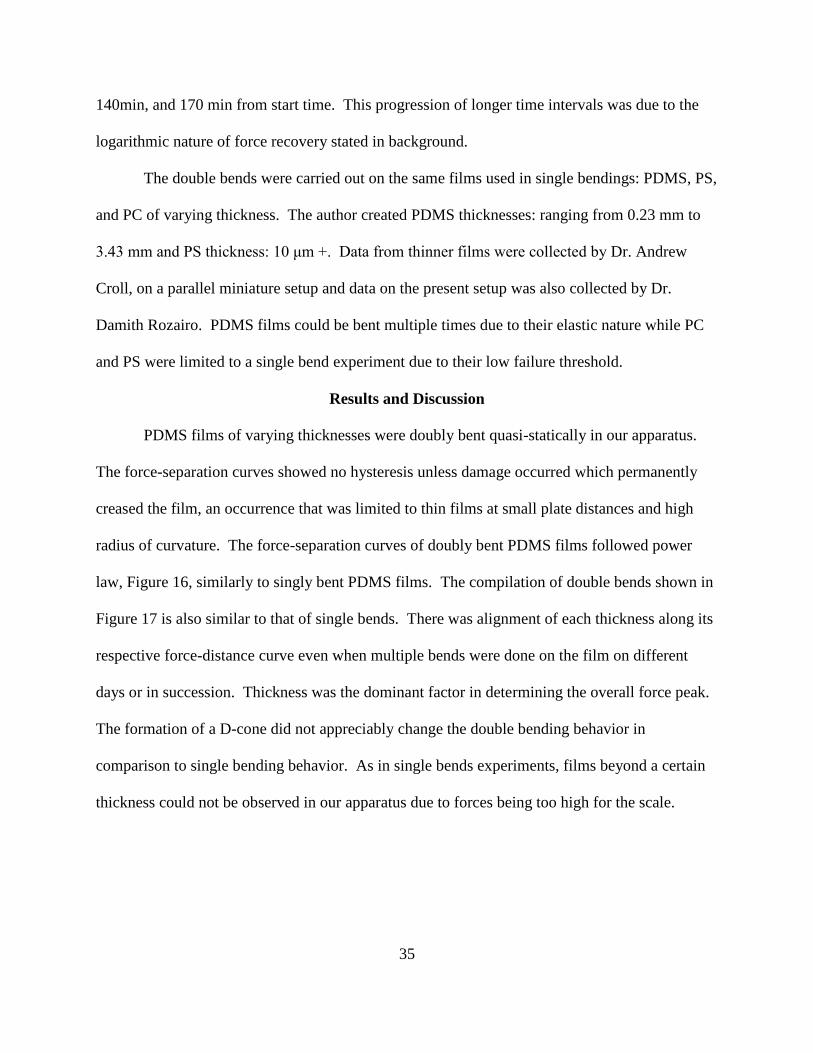
35
140min, and 170 min from start time. This progression of longer time intervals was due to the
logarithmic nature of force recovery stated in background.
The double bends were carried out on the same films used in single bendings: PDMS, PS,
and PC of varying thickness. The author created PDMS thicknesses: ranging from 0.23 mm to
3.43 mm and PS thickness: 10 μm +. Data from thinner films were collected by Dr. Andrew
Croll, on a parallel miniature setup and data on the present setup was also collected by Dr.
Damith Rozairo. PDMS films could be bent multiple times due to their elastic nature while PC
and PS were limited to a single bend experiment due to their low failure threshold.
Results and Discussion
PDMS films of varying thicknesses were doubly bent quasi-statically in our apparatus.
The force-separation curves showed no hysteresis unless damage occurred which permanently
creased the film, an occurrence that was limited to thin films at small plate distances and high
radius of curvature. The force-separation curves of doubly bent PDMS films followed power
law, Figure 16, similarly to singly bent PDMS films. The compilation of double bends shown in
Figure 17 is also similar to that of single bends. There was alignment of each thickness along its
respective force-distance curve even when multiple bends were done on the film on different
days or in succession. Thickness was the dominant factor in determining the overall force peak.
The formation of a D-cone did not appreciably change the double bending behavior in
comparison to single bending behavior. As in single bends experiments, films beyond a certain
thickness could not be observed in our apparatus due to forces being too high for the scale.

36
Figure 16. A typical force-separation curve for a doubly bent 10:1 PDMS sample of dimensions
length 79.62 mm, width 73.05 mm, and thickness 0.67 mm in the single bend geometry. Note the
lack of appreciable hysteresis as the curve shows both advancing and receding. The power law
fit equation for this graph is 𝑦 = 0.29𝑥−2.
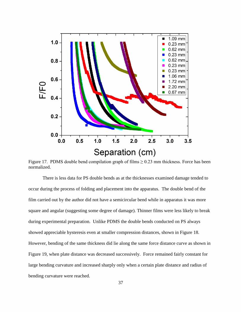
37
Figure 17. PDMS double bend compilation graph of films ≥ 0.23 mm thickness. Force has been
normalized.
There is less data for PS double bends as at the thicknesses examined damage tended to
occur during the process of folding and placement into the apparatus. The double bend of the
film carried out by the author did not have a semicircular bend while in apparatus it was more
square and angular (suggesting some degree of damage). Thinner films were less likely to break
during experimental preparation. Unlike PDMS the double bends conducted on PS always
showed appreciable hysteresis even at smaller compression distances, shown in Figure 18.
However, bending of the same thickness did lie along the same force distance curve as shown in
Figure 19, when plate distance was decreased successively. Force remained fairly constant for
large bending curvature and increased sharply only when a certain plate distance and radius of
bending curvature were reached.
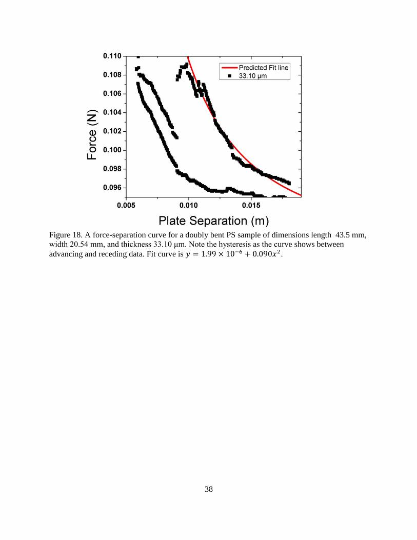
38
Figure 18. A force-separation curve for a doubly bent PS sample of dimensions length 43.5 mm,
width 20.54 mm, and thickness 33.10 μm. Note the hysteresis as the curve shows between
advancing and receding data. Fit curve is 𝑦 = 1.99 × 10⁻⁶ + 0.090𝑥2.
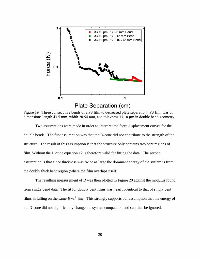
39
Figure 19. Three consecutive bends of a PS film to decreased plate separation. PS film was of
dimensions length 43.5 mm, width 20.54 mm, and thickness 33.10 μm in double bend geometry.
Two assumptions were made in order to interpret the force displacement curves for the
double bends. The first assumption was that the D-cone did not contribute to the strength of the
structure. The result of this assumption is that the structure only contains two bent regions of
film. Without the D-cone equation 12 is therefore valid for fitting the data. The second
assumption is that since thickness was twice as large the dominant energy of the system is from
the doubly thick bent region (where the film overlaps itself).
The resulting measurement of 𝐵 was then plotted in Figure 20 against the modulus found
from single bend data. The fit for doubly bent films was nearly identical to that of singly bent
films in falling on the same 𝐵~𝑡3 line. This strongly supports our assumption that the energy of
the D-cone did not significantly change the system compaction and can thus be ignored.
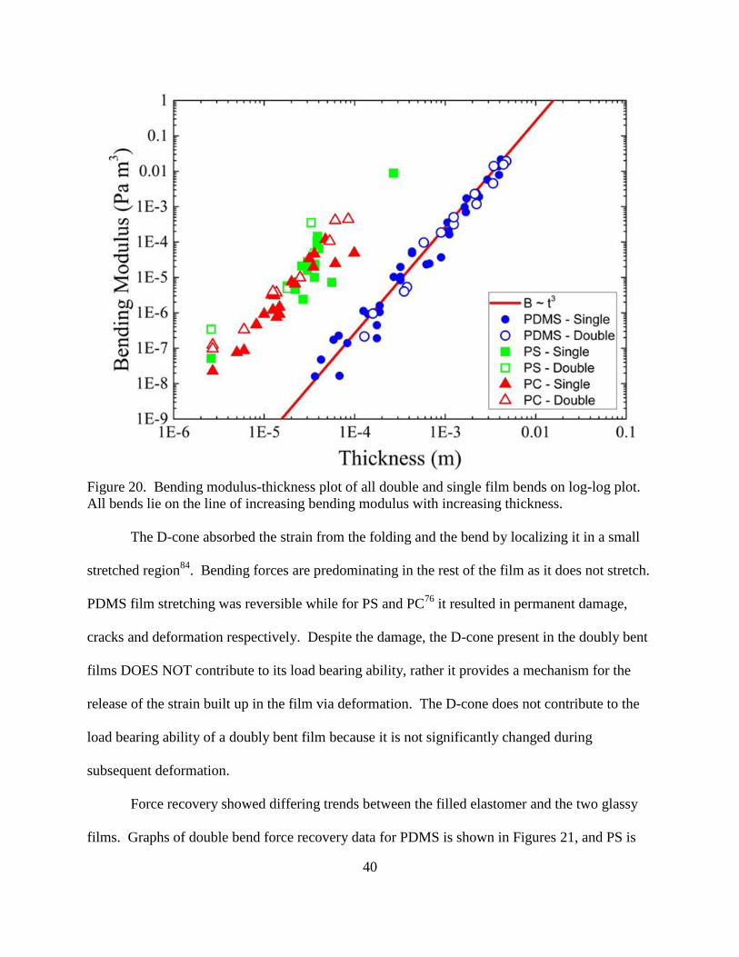
40
Figure 20. Bending modulus-thickness plot of all double and single film bends on log-log plot.
All bends lie on the line of increasing bending modulus with increasing thickness.
The D-cone absorbed the strain from the folding and the bend by localizing it in a small
stretched region84
. Bending forces are predominating in the rest of the film as it does not stretch.
PDMS film stretching was reversible while for PS and PC76
it resulted in permanent damage,
cracks and deformation respectively. Despite the damage, the D-cone present in the doubly bent
films DOES NOT contribute to its load bearing ability, rather it provides a mechanism for the
release of the strain built up in the film via deformation. The D-cone does not contribute to the
load bearing ability of a doubly bent film because it is not significantly changed during
subsequent deformation.
Force recovery showed differing trends between the filled elastomer and the two glassy
films. Graphs of double bend force recovery data for PDMS is shown in Figures 21, and PS is
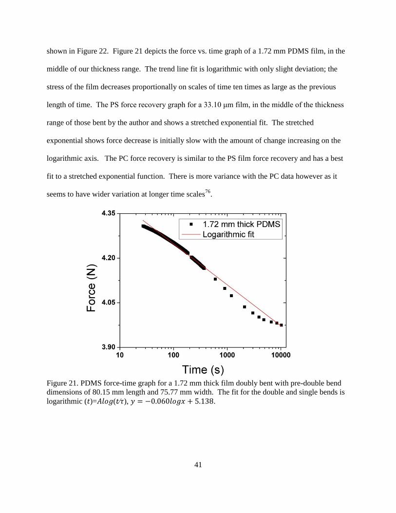
41
shown in Figure 22. Figure 21 depicts the force vs. time graph of a 1.72 mm PDMS film, in the
middle of our thickness range. The trend line fit is logarithmic with only slight deviation; the
stress of the film decreases proportionally on scales of time ten times as large as the previous
length of time. The PS force recovery graph for a 33.10 μm film, in the middle of the thickness
range of those bent by the author and shows a stretched exponential fit. The stretched
exponential shows force decrease is initially slow with the amount of change increasing on the
logarithmic axis. The PC force recovery is similar to the PS film force recovery and has a best
fit to a stretched exponential function. There is more variance with the PC data however as it
seems to have wider variation at longer time scales76
.
Figure 21. PDMS force-time graph for a 1.72 mm thick film doubly bent with pre-double bend
dimensions of 80.15 mm length and 75.77 mm width. The fit for the double and single bends is
logarithmic (𝑡)=𝐴𝑙𝑜𝑔(𝑡∕𝜏), 𝑦 = −0.060𝑙𝑜𝑔𝑥 + 5.138.

42
Figure 22. A PS force vs. time graph of a 33.10 μm film with pre-bend length of 43.5 mm and
width of 20.54 mm. The fit for the double and single bends lies along a
𝑦 = 1.72 𝑒𝑥𝑝 (−(𝑥12500⁄ )
0.55
) stretched exponential curve.
All of the doubly bent and singly bent samples for force recovery data were then
compiled onto single graphs; force recovery of PDMS is shown in Figure 23 and force recovery
of PS in Figure 24. All thicknesses of PDMS displayed the same trend after normalization by the
force measured at 40 seconds. The differences in the force recovery behavior of PS can be
attributed to initial plate separation and initial force. Smaller plate separation and higher initial
force had more rapid decrease in force with respect to time. This means that we saw a more
rapid decrease in force at smaller bending radius of curvatures. PC force recovery was carried
out for a range of thicknesses. The PC response was similar to that of PS76
.

43
Figure 23. All samples of PDMS force recovery for single and double bends, normalized. There
is no response distinction between the single bends and double bends or between thicknesses.
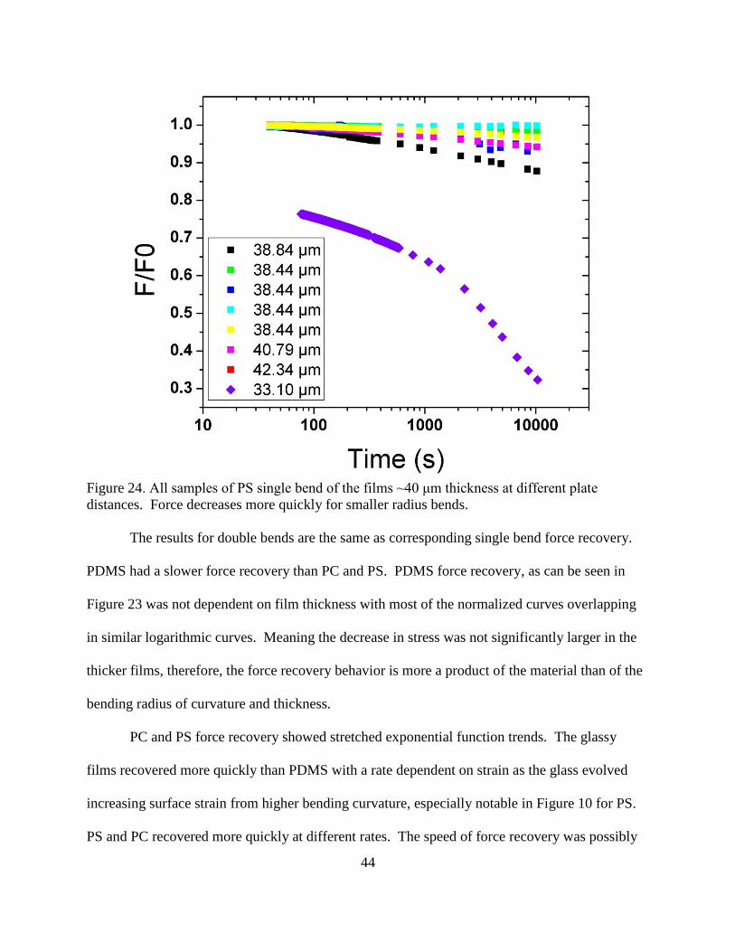
44
Figure 24. All samples of PS single bend of the films ~40 μm thickness at different plate
distances. Force decreases more quickly for smaller radius bends.
The results for double bends are the same as corresponding single bend force recovery.
PDMS had a slower force recovery than PC and PS. PDMS force recovery, as can be seen in
Figure 23 was not dependent on film thickness with most of the normalized curves overlapping
in similar logarithmic curves. Meaning the decrease in stress was not significantly larger in the
thicker films, therefore, the force recovery behavior is more a product of the material than of the
bending radius of curvature and thickness.
PC and PS force recovery showed stretched exponential function trends. The glassy
films recovered more quickly than PDMS with a rate dependent on strain as the glass evolved
increasing surface strain from higher bending curvature, especially notable in Figure 10 for PS.
PS and PC recovered more quickly at different rates. The speed of force recovery was possibly

45
due to relaxation mechanisms of the amorphous molecules rearranging. The force recovery of
singly and doubly bent films exhibits the same behaviors for all three films in comparison to
single bends.
All three types of film experienced failure at high loads or following aging. Thinner
films of PDMS experienced permanent creasing under large constant loads and small plate
distances. Older PDMS films that had been subjected to force recovery numerous times and
asymmetric films also experienced fracture failures. PS cracked under too high of loads with
damage in the form of crazing or fracture breaking the film cleanly in half in some instances.
When PS cracked before the final displacement and load was reached, in some instances cracks
increased when left overnight. These failing samples were excluded from data as they had other
factors that altered the strain distribution under stress.
Conclusion
Our experiment aimed to increase the literature and understanding of the effect of D-
cones in polymeric materials (PDMS, PC, PS) on their stress-strain response and how the
systems recovered over time at constant loads. We created doubly bent films and carried out
force-displacement compression testing in the same manner as the singly bent films described in
chapter 1. Data was fit with predictions in order to determine differences. No differences were
observed leading to the conclusion that the D-cone is not load bearing and does not affect
compaction. Force recovery was then carried out on the three polymeric systems in double bend
geometries when applicable. PDMS recovered logarithmically while PS and PC76
recovered
much faster in a stretched exponential fashion possibly accounted for by molecular arrangement.
The D-cone did not contribute noticeably to force recovery as double bend and single bend
samples of PDMS exhibited similar force recovery curves. Future work remaining to be done is

46
expansion on the stress-strain behavior of the thicker glassy films though single bends, double
bends, and force recovery and more specifications of the D-cone geometry for each of the model
materials.
47
CHAPTER 3. MICROGEL PARTICLES FROM TRIBLOCK COPOLYMER PS-PAA-PS
Background
Microgel particles and nanogel particles are smart responsive materials used currently in
pharmaceuticals as capsules for drug delivery89,90
, medical imaging91
, coatings, printing
applications89
, pollution control systems, catalysis90
, food engineering, cosmetics92
, and personal
care products91
. Microgels are defined as micro or nanoscale cross-linked latex particles89
or
colloidal polymer networks which encase a solvent93
in a polymer mesh and respond to external
stimuli such as temperature, pH, magnetism, electrical fields, salt, light, ultrasound, and solvent
chemistry94
. Microgel particles have combined polymer and colloid chemistry, properties, and
physics. The flexible nature of microgels make them able to compress and pack together in high
densities89,91,95
. The potential exists for expanding the applications of these structures into other
uses and expanding their abilities in current usage through tuning environmental responsiveness
and structure complexity89,93,96,97
.
Gels are 3D macroscopic networks of connected molecular subunits that have non-zero
shear modulus, are structurally disordered and may contain high liquid volume fractions of
solvent. Macroscopic properties of gels change based on the number of bonds and type of bonds
between molecules which can be chemical or physical with physically bonded gels being
thermoreversible98
. Mechanical properties can be improved in macrogels through modifications
of architecture or the addition of inorganic particles incorporated into the gel matrix adding
additional response ability to stimuli such as electricity and magnetism. However, there are
many clear advantages to microgel particles. Microgel particles have been found to swell much
faster than macrogels by as much as eight orders of magnitude99
and have higher exchange rate
at the surface; a property useful in drug delivery applications along with the biotechnology
48
advantages of colloids100
. Microgel particles have the advantages of gels, such as high solvent
absorbance, yield stress89
, and softness, without some of the disadvantages: hysteresis in
transition between swollen and non-swollen states, irreversible expansion or compression, and
slow absorbance or diffusion rates. In macrogels liquid taken in results in tension, the fluid is
released under compression101
force; microgel particles do not release their solvent under
compression; they are softer and more deformable. Microgels are able to squeeze through small
spaces, and undergo changes in volume under stress102
without sustaining the damage91
that a
macroscale hydrogel would103
. The mechanical properties are sometimes large enough to be
measurable through micropipette aspiration where a micropipette is used to aspirate a particle
into a micropipette. The deformation and suction force provide information on particle
elasticity, and possible lysis points104
. Microgels have lower viscosity within the same occupied
space compared to hard sphere particles, have high water/solvent content, elasticity, and the high
surface area to volume ratio of a colloidal particle89
. Generally below micrometer size diameters
microgels remain colloidal and do not precipitate out of solution even during swelling, subject
only to Brownian diffusion from thermal energy101
.
One of the biggest advantages of microgel particles is their swelling from external
stimuli, the polymers of the particle expand outward and the particle enlarges, changing the
dimensions of a particle reversibly (Figure 25). Changes in size and other microgel properties
lead to behavior and properties that differ from that of traditional hard sphere particles and
colloidal systems91,105
. Swelling is influenced by osmotic pressure differentials between the
external polymer segments, those interacting with surrounding solvent and internal polymer
segments in microgel interior. During expansion previously buried regions are exposed97
in
substantial numbers, these newly exposed polymer regions can interact with the surrounding
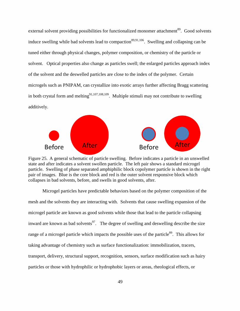
49
external solvent providing possibilities for functionalized monomer attachment89
. Good solvents
induce swelling while bad solvents lead to compaction89,91,106
. Swelling and collapsing can be
tuned either through physical changes, polymer composition, or chemistry of the particle or
solvent. Optical properties also change as particles swell; the enlarged particles approach index
of the solvent and the deswelled particles are close to the index of the polymer. Certain
microgels such as PNIPAM, can crystallize into exotic arrays further affecting Bragg scattering
in both crystal form and melting91,107,108,109
. Multiple stimuli may not contribute to swelling
additively.
Figure 25. A general schematic of particle swelling. Before indicates a particle in an unswelled
state and after indicates a solvent swollen particle. The left pair shows a standard microgel
particle. Swelling of phase separated amphiphilic block copolymer particle is shown in the right
pair of images. Blue is the core block and red is the outer solvent responsive block which
collapses in bad solvents, before, and swells in good solvents, after.
Microgel particles have predictable behaviors based on the polymer composition of the
mesh and the solvents they are interacting with. Solvents that cause swelling expansion of the
microgel particle are known as good solvents while those that lead to the particle collapsing
inward are known as bad solvents97
. The degree of swelling and deswelling describe the size
range of a microgel particle which impacts the possible uses of the particle89
. This allows for
taking advantage of chemistry such as surface functionalization: immobilization, tracers,
transport, delivery, structural support, recognition, sensors, surface modification such as hairy
particles or those with hydrophilic or hydrophobic layers or areas, rheological effects, or

50
saccharine coverage110
. Proteins for transport and biomineralization, can be complexed into the
structure to add functionality and stability104
.
Microgel particles are versatile due to their deformability and can be of use in emulsions
and foams which maintain high surface tensions111,112
. Concentration can be increased with
volume fractions close to 1, forming pastes113,114
due to a unique relationship between volume
fraction and polymer size89
. Hard particles exhibit characteristic rheology of increased viscosity
with increased particle volume fraction115
. Increased volume fraction of crosslinked polymeric
nanoparticles, however, exhibit the opposite rheology, high volume fractions have decreasing
viscosity (shear thinning) attributable to increased free volume and improved energy
dissipation116
. The particles can also be used to co-assemble other nanoparticles from inorganic
constituents due to the ability for smaller particles and polymers to pass through the polymer
mesh shells117,118,119
. The inclusion of smaller particles and polymers can affect the osmotic
pressure balance or solvent-particle interactions89
.
The first reported microgel particles were crosslinked divinylbenzene (DVB) of narrow
size dispersion synthesized in 1935 by Staudinger and Husemann89
. Since 1935 numerous other
polymers have been found to effectively form microgel particles such as polystyrene (PS), and
poly(N-isopropylacrylamide) (PNIPAM). In certain polymers such as polyacrylic acid (PAA),
pH can stimulate swelling via a reversible proton exchange with solvent/water from a pendent
group that is either acidic or basic101
. The electrostatic interactions from charged groups increase
inherent stability89
even as they swell. This aligns with other studies where small changes can
have large effects in microgel particle outcomes120
. Addition of excess electrolytic polymer such
as PAA to microgel solutions had lowered osmotic pressure and deswelling effects; when PAA
was also a component of the microgel particles swelling occurred at higher pH values. Charged
51
groups along polymer backbone affect microgel stability and osmotic pressure stabilizations89,97
.
Addition of polyelectrolytes, therefore, gives additional functionality and versatility to microgel
particle systems89
including responsive polymer conjugates for biological molecules such as
antibodies and enzymes94
.
Microgel particles can be formed in several ways, all of which follow one of two general
pathways: disintegration of larger structures through breaking of interparticle bonds or
aggregation in high solution concentrations, promoting noncovalent interactions104
. The most
common methods of microgel synthesis are the result of direct synthesis emulsion
polymerization121,122
, anionic polymerization123
, inverse micro-emulsions polymerization89,124
followed by cross-linking of the polymer chain125
often through photo catalysis, and
heterogeneous polymerization with bifunctional or multifunctional cross-linkers126,127
, and self-
assembly via kinetic channels. Kinetic channels such as self- assembly result from processes
such as solvent mixing128
, emulsification129
, or crystallization of blocks96,130
that lead to
spontaneous demixing from the natural phase separation of unlike polymer blocks to increase
stability96
.
Kinetic control can be achieved through either solvent-directed manipulation or acid/
base directed complexation for block copolymers with suitable chemically compatible groups
such as multifunctional organic amines and hydrophilic water compatible PAA blocks96
. Kinetic
controlled self-assembly through solvent mixing uses principles such as co-non-solvency where
a mixture of solvents that are usually good solvents for a polymer are combined to produce a bad
solvent for the polymer131
. Co-non-solvency leads to a narrower particle size distribution as
particle size uniformity has been found to be less achievable in good solvents due to low
electrostatic stabilization since radical sites and pendant vinyl group interact between
52
neighboring polymer chains which grow the polymer networks sporadically leading to different
size distributions89
. If a proper balance of solvents is not achieved frustration of the forming
particle can lead to saddle shapes and concentric onion morphologies104
.
Amphiphilic block copolymers are especially useful in kinetic control adding the stability
of charge and forming aggregations of specific morphologies132
. The hydrophobic regions
aggregate in polar solvents and swell while in non-polar solvents while hydrophilic regions
interact favorably with polar solvents, and aggregate in organic solvents. Phase separation and
aggregation of unlike polymers, such as hydrophilic-hydrophobic interactions, form particles
with three regions the insoluble core, a wall and a soluble corona120
. Multiple morphologies are
possible including inverted structures based on the spontaneous membrane curvature formed and
the shape of lowest energy as well as vesicular types, those with a hollow internal cavity, which
can hold solutes, dye, macromolecules and proteins that could be utilized in drug delivery and
other applications104,106,120
. If the copolymer used to make a microgel has more than two blocks
multicompartment nanostructures133,134,135,136
can be formed.
Here we use a guided self-assembly method carried out with ratios of good and bad
solvent for a kinetically advantageous polymer aggregate. This approach has been carried out by
other groups137
where a blending of high molecular weight polymer solution in an aqueous
medium produced nanoparticles of a single geometry that demixed into vesicles and
multicompartment nanoparticles respectively. Experimentally for polystyrene-block-poly(
acrylic acid) (PS-b-PAA) diblock copolymer the microgel morphology is influenced by the
length of PS, the hydrophobic block138
. Phase separation in solvents known as “kinetic trapping”
is the phase separation of water mixed with organic solvent in solution which can produce a
polymersome, an artificial polymer vesicle139
.
53
Physical qualities, capabilities, geometries, and methods of formation are a growing area
of research. The purpose of this work is to self-assemble electrolytic microgel particles from a
model triblock copolymer through the use of solvent mixing and examine the resulting structural
morphology, physical properties, and particle responsiveness. Specifically, we created particles
from ABA triblock copolymers, which have been found to create micelles94
of PS-PAA-PS
through self-assembly from solvent mixing. The polymer used was a triblock of (PS) and (PAA)
due to their high availability, ability to be synthesized in high purity, known properties, and the
electrolytic effects of PAA combined with the hydrophobic effects of PS140
. The triblock
copolymer consists of two PS end blocks with a longer chain of PAA in the middle. PS was
chosen as it is well-studied hydrophobic polymer that swells in aromatic organic solvents and the
PS also adds stability due to its high glass temperature76
. PAA was chosen for its valuable
properties of pH responsiveness and biocompatibility141
. PAA is biocompatible with carboxyl
groups that provide a built in responsiveness to pH142
; PAA is also an acid which provides the
opportunity for examining interactions with different solvents and salts.
Previous works have shown that PAA and PS block copolymers form structures upon
dialysis with water. In the case of a diblock copolymer, as carried out by Li et al., a micelle was
formed when the diblock was dissolved in water and DMF solution due to the amphiphilic
chemical nature of the polymer which forms hydrogen bonds with the water143
or in THF, water,
and DMF solvent120,144,145
. Particle size is largely dependent on the length of the PAA block of
the copolymer; longer PAA blocks have higher water affinity forming more hydrogen bonds
which increases the surface tension and decreases interfacial tension between the PAA segments
and the PS segments, lowering free energy98,104
. Aromatic organic solvent such as THF89
fluidizes and swells PS while the addition of water causes the chains to aggregate and solidify104
.
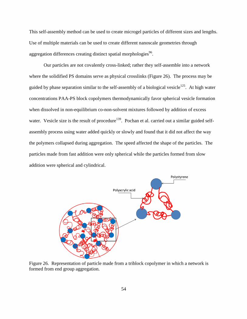
54
This self-assembly method can be used to create microgel particles of different sizes and lengths.
Use of multiple materials can be used to create different nanoscale geometries through
aggregation differences creating distinct spatial morphologies96
.
Our particles are not covalently cross-linked; rather they self-assemble into a network
where the solidified PS domains serve as physical crosslinks (Figure 26). The process may be
guided by phase separation similar to the self-assembly of a biological vesicle125
. At high water
concentrations PAA-PS block copolymers thermodynamically favor spherical vesicle formation
when dissolved in non-equilibrium co-non-solvent mixtures followed by addition of excess
water. Vesicle size is the result of procedure139
. Pochan et al. carried out a similar guided self-
assembly process using water added quickly or slowly and found that it did not affect the way
the polymers collapsed during aggregation. The speed affected the shape of the particles. The
particles made from fast addition were only spherical while the particles formed from slow
addition were spherical and cylindrical.
Figure 26. Representation of particle made from a triblock copolymer in which a network is
formed from end group aggregation.

55
Theory
Classically microgel particles have been compared to hard spheres; however, the
comparison is flawed. Depending on the curvature of the particle, the volume fraction, and the
particle chemistry146
the microgel particle system has been shown to have unique qualities vastly
different from those of a hard sphere system. In 1D microgel particles and hard spheres behave
as linear arrays of spheres subject to repulsion104,147
; in 2D microgel particles behave more like
liquids104
while hard spheres cannot fully occupy a space and form close packing hexagonal
structures. In 3D hard sphere system particles cannot occupy spaces already occupied by
neighbor particles; as the number of particles increases the order increases. In general, the
spheres form close packed structures which do not fully occupy a space. Microgel particles can
pack to higher densities in 3D than hard spheres due to their lower repulsion forces147
and
malleable softness which results in different properties. As mentioned in the background section
microgel particles exhibit non-Einstein viscosity and shear thinning89
in colloidal suspension
which allows for more dense packing than possible in hard spheres89,116
and gives them liquid-
like behavior even at high volume fractions. The decreased viscosity and ability to densely pack
affects the thermodynamics of the system, for example altering crystallization temperatures and
glass transitions95
. The softer microgel particles are less fragile, or less prone to breaking, at the
transition temperatures than comparable hard spheres which are more brittle. The microgels also
showed stronger tendency towards suspension behavior unless protonated or affected by external
stimuli compared to a similar hard sphere91
.
The underlying physics of microgel particles remains under study. Past and current
theories of microgel particles mechanical properties and swelling remain insufficient to explain
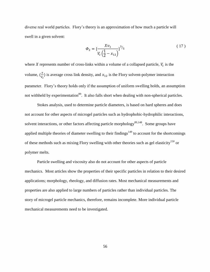
56
diverse real world particles. Flory’s theory is an approximation of how much a particle will
swell in a given solvent:
𝛷2 = {
𝛸𝑣1
𝑉𝑐 (12 − 𝑥12)
}3
5⁄ ( 17 )
where 𝑋 represents number of cross-links within a volume of a collapsed particle, 𝑉𝑐 is the
volume, (𝑥
𝑉𝑐) is average cross link density, and 𝑥12 is the Flory solvent-polymer interaction
parameter. Flory’s theory holds only if the assumption of uniform swelling holds, an assumption
not withheld by experimentation89
. It also falls short when dealing with non-spherical particles.
Stokes analysis, used to determine particle diameters, is based on hard spheres and does
not account for other aspects of microgel particles such as hydrophobic-hydrophilic interactions,
solvent interactions, or other factors affecting particle morphology89,148
. Some groups have
applied multiple theories of diameter swelling to their findings149
to account for the shortcomings
of these methods such as mixing Flory swelling with other theories such as gel elasticity150
or
polymer melts.
Particle swelling and viscosity also do not account for other aspects of particle
mechanics. Most articles show the properties of their specific particles in relation to their desired
applications; morphology, rheology, and diffusion rates. Most mechanical measurements and
properties are also applied to large numbers of particles rather than individual particles. The
story of microgel particle mechanics, therefore, remains incomplete. More individual particle
mechanical measurements need to be investigated.
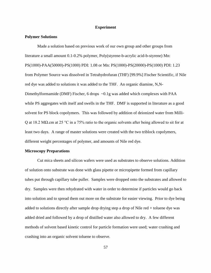
57
Experiment
Polymer Solutions
Made a solution based on previous work of our own group and other groups from
literature a small amount 0.1-0.2% polymer, Poly(styrene-b-acrylic acid-b-styrene) Mn:
PS(1000)-PAA(50000)-PS(1000) PDI: 1.08 or Mn: PS(1000)-PS(20000)-PS(1000) PDI: 1.23
from Polymer Source was dissolved in Tetrahydrofuran (THF) [99.9%] Fischer Scientific, if Nile
red dye was added to solutions it was added to the THF. An organic diamine, N,N-
Dimethylformamide (DMF) Fischer, 6 drops ~0.1g was added which complexes with PAA
while PS aggregates with itself and swells in the THF. DMF is supported in literature as a good
solvent for PS block copolymers. This was followed by addition of deionized water from Milli-
Q at 18.2 MΩ.cm at 25 °C in a 75% ratio to the organic solvents after being allowed to sit for at
least two days. A range of master solutions were created with the two triblock copolymers,
different weight percentages of polymer, and amounts of Nile red dye.
Microscopy Preparations
Cut mica sheets and silicon wafers were used as substrates to observe solutions. Addition
of solution onto substrate was done with glass pipette or micropipette formed from capillary
tubes put through capillary tube puller. Samples were dropped onto the substrates and allowed to
dry. Samples were then rehydrated with water in order to determine if particles would go back
into solution and to spread them out more on the substrate for easier viewing. Prior to dye being
added to solutions directly after sample drop drying step a drop of Nile red + toluene dye was
added dried and followed by a drop of distilled water also allowed to dry. A few different
methods of solvent based kinetic control for particle formation were used; water crashing and
crashing into an organic solvent toluene to observe.
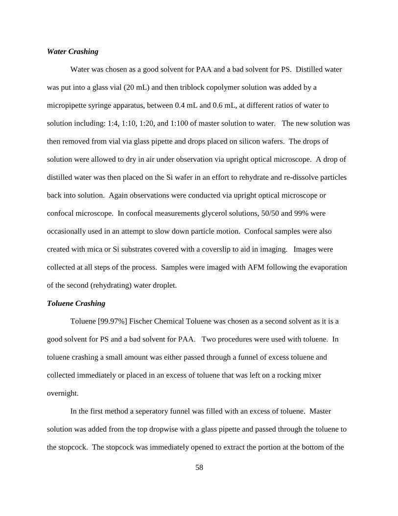
58
Water Crashing
Water was chosen as a good solvent for PAA and a bad solvent for PS. Distilled water
was put into a glass vial (20 mL) and then triblock copolymer solution was added by a
micropipette syringe apparatus, between 0.4 mL and 0.6 mL, at different ratios of water to
solution including: 1:4, 1:10, 1:20, and 1:100 of master solution to water. The new solution was
then removed from vial via glass pipette and drops placed on silicon wafers. The drops of
solution were allowed to dry in air under observation via upright optical microscope. A drop of
distilled water was then placed on the Si wafer in an effort to rehydrate and re-dissolve particles
back into solution. Again observations were conducted via upright optical microscope or
confocal microscope. In confocal measurements glycerol solutions, 50/50 and 99% were
occasionally used in an attempt to slow down particle motion. Confocal samples were also
created with mica or Si substrates covered with a coverslip to aid in imaging. Images were
collected at all steps of the process. Samples were imaged with AFM following the evaporation
of the second (rehydrating) water droplet.
Toluene Crashing
Toluene [99.97%] Fischer Chemical Toluene was chosen as a second solvent as it is a
good solvent for PS and a bad solvent for PAA. Two procedures were used with toluene. In
toluene crashing a small amount was either passed through a funnel of excess toluene and
collected immediately or placed in an excess of toluene that was left on a rocking mixer
overnight.
In the first method a seperatory funnel was filled with an excess of toluene. Master
solution was added from the top dropwise with a glass pipette and passed through the toluene to
the stopcock. The stopcock was immediately opened to extract the portion at the bottom of the

59
funnel, which should contain any newly formed particles. The toluene solution was then applied
directly to substrate dropwise with a glass pipette; toluene drops dried before addition of
subsequent drops. Vials with too much toluene were placed in a fume hood to allow the
evaporation of the excess.
The second toluene crashing method involved prolonged mixing in toluene. A 20 mL
vial was filled to almost the top with toluene; a small amount of copolymer solution was added
(5-15 drops from a glass pipette). Additional toluene was then added to fill the vial fully; the
cap of the vial was then screwed on and it was immediately placed on a wave motion lab mixer
for 24 hours. After the 24 hour period the vial was removed and the sample was taken as quickly
as possible from the bottom of the vial and placed dropwise onto substrate via glass pipette.
Toluene was allowed to dry in between drops. Images of the resulting particles were collected
with an upright optical microscope. A drop of water was added to rehydrate particles and was
accompanied by more observations and imaging. At times a hot stage was used to speed the
drying during the rehydration step.
Results and Discussion
PS-PAA-PS triblock was dissolved in solutions of 3:1 water to organic ratio, at other
ratios the master solutions showed undissolved chunks or visible lines in solution. This finding
was in keeping with literature and some previous work by Rozairo et al151
. Some master
solutions were cloudy with larger polymer concentrations, possibly indicating micelle formation.
Triblock did not form particles in solution without further kinetic solvent co-non-solvency this
was evident from drying master solution alone on a Si wafer as shown in Figure 27. Even after
rehydration dried out master solution formed large clumps of polymer of film-like blobs which
swelled with water addition and linear polymer. The large amount of polymer on the wafer
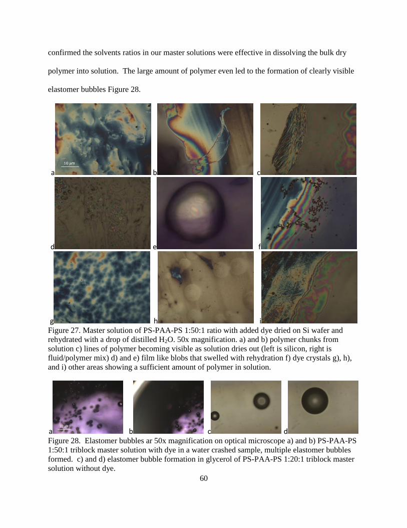
60
confirmed the solvents ratios in our master solutions were effective in dissolving the bulk dry
polymer into solution. The large amount of polymer even led to the formation of clearly visible
elastomer bubbles Figure 28.
a b c
d e f
g h i Figure 27. Master solution of PS-PAA-PS 1:50:1 ratio with added dye dried on Si wafer and
rehydrated with a drop of distilled H2O. 50x magnification. a) and b) polymer chunks from
solution c) lines of polymer becoming visible as solution dries out (left is silicon, right is
fluid/polymer mix) d) and e) film like blobs that swelled with rehydration f) dye crystals g), h),
and i) other areas showing a sufficient amount of polymer in solution.
a b c d Figure 28. Elastomer bubbles ar 50x magnification on optical microscope a) and b) PS-PAA-PS
1:50:1 triblock master solution with dye in a water crashed sample, multiple elastomer bubbles
formed. c) and d) elastomer bubble formation in glycerol of PS-PAA-PS 1:20:1 triblock master
solution without dye.
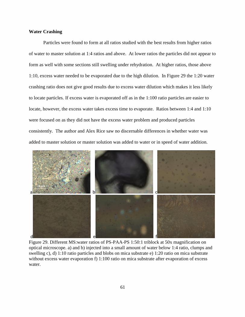
61
Water Crashing
Particles were found to form at all ratios studied with the best results from higher ratios
of water to master solution at 1:4 ratios and above. At lower ratios the particles did not appear to
form as well with some sections still swelling under rehydration. At higher ratios, those above
1:10, excess water needed to be evaporated due to the high dilution. In Figure 29 the 1:20 water
crashing ratio does not give good results due to excess water dilution which makes it less likely
to locate particles. If excess water is evaporated off as in the 1:100 ratio particles are easier to
locate, however, the excess water takes excess time to evaporate. Ratios between 1:4 and 1:10
were focused on as they did not have the excess water problem and produced particles
consistently. The author and Alex Rice saw no discernable differences in whether water was
added to master solution or master solution was added to water or in speed of water addition.
a b c
d e f Figure 29. Different MS:water ratios of PS-PAA-PS 1:50:1 triblock at 50x magnification on
optical microscope. a) and b) injected into a small amount of water below 1:4 ratio, clumps and
swelling c), d) 1:10 ratio particles and blobs on mica substrate e) 1:20 ratio on mica substrate
without excess water evaporation f) 1:100 ratio on mica substrate after evaporation of excess
water.

62
During drying most samples formed concentrated central areas which were too
concentrated and tall to properly image without further treatment. To spread the particles out
heat drying, washers sonicated in acetone, and water hydration were found to be effective, Figure
30. The addition of a hot stage to the sample drying process resulted in more spread out
particles. The particles were spatially separated; however, the morphology of the resultant
particles seemed different than samples allowed to dry in ambient temperatures. Placing the
sample in the center of a washer in order to draw out the corners of the solution as it dried was
somewhat effective, however, some solution would go underneath of the washer resulting in less
particles on the undisturbed substrate. Water rehydration alone did not spread out the particles
sufficiently unless pipette was used to physically move them or small amount was moved to
another location.
a b c
d e f Figure 30. PS-PAA-PS 1:50:1 triblock a), b), c) 1:10 ratio water crashing and heat assisted
solvent evaporation at 50x magnification. d) sample dried in center of washer at 5x
magnification e) and f) at 50x magnification.
Samples showed some difference in overall morphology between the different length
triblock copolymers and the different master solutions. Figure 31 shows the morphology of

63
different solutions at 1:4 ratios. AFM was used to image morphology and texture to determine if
the polymer formed discrete particles, film-like blobs, or disorganized polymer clumps. The
AFM provided shapes of formations and size ranges. Tapping mode was used in order to
distinguish between the soft PAA blocks and the harder solidified PS aggregate blocks. Longer
triblock copolymer, that at 1:50:1 ratio, showed consistent morphology as shown in Figure 32
where the particles appear as round flattened pancakes which is in keeping with literature
observations89
of microgel spheres upon solvent evaporation. The dye also did not appear to
have any effect on morphology. The shorter polymer showed a more diverse irregular
morphology between solutions although all appeared to make particles.
a b c
d e f Figure 31. PS-PAA-PS 1:50:1 with dye at 1:4 ratio MS: water dried and rehydrated a), b), c) are
at 5x magnification d), e), and f) are at 50x magnification.
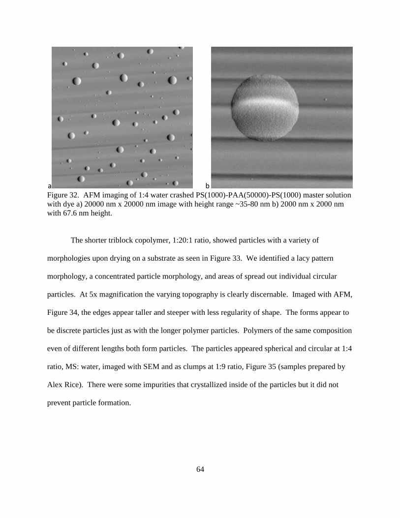
64
a b Figure 32. AFM imaging of 1:4 water crashed PS(1000)-PAA(50000)-PS(1000) master solution
with dye a) 20000 nm x 20000 nm image with height range ~35-80 nm b) 2000 nm x 2000 nm
with 67.6 nm height.
The shorter triblock copolymer, 1:20:1 ratio, showed particles with a variety of
morphologies upon drying on a substrate as seen in Figure 33. We identified a lacy pattern
morphology, a concentrated particle morphology, and areas of spread out individual circular
particles. At 5x magnification the varying topography is clearly discernable. Imaged with AFM,
Figure 34, the edges appear taller and steeper with less regularity of shape. The forms appear to
be discrete particles just as with the longer polymer particles. Polymers of the same composition
even of different lengths both form particles. The particles appeared spherical and circular at 1:4
ratio, MS: water, imaged with SEM and as clumps at 1:9 ratio, Figure 35 (samples prepared by
Alex Rice). There were some impurities that crystallized inside of the particles but it did not
prevent particle formation.
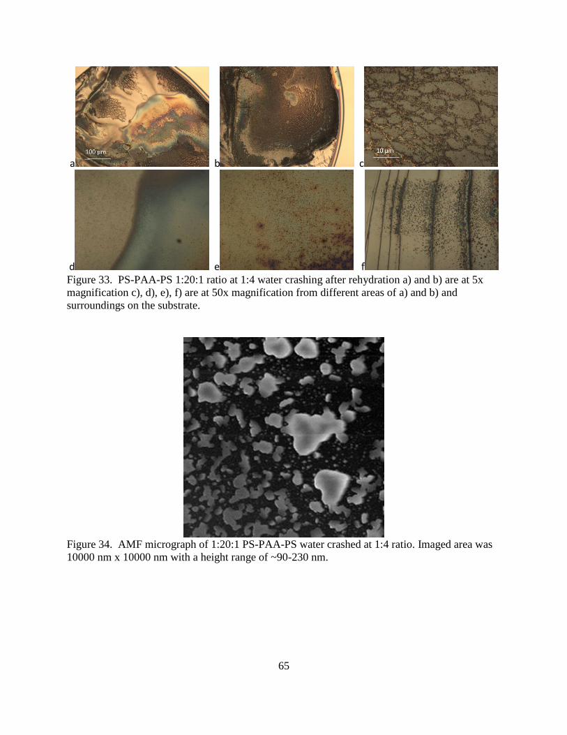
65
a b c
d e f Figure 33. PS-PAA-PS 1:20:1 ratio at 1:4 water crashing after rehydration a) and b) are at 5x
magnification c), d), e), f) are at 50x magnification from different areas of a) and b) and
surroundings on the substrate.
Figure 34. AMF micrograph of 1:20:1 PS-PAA-PS water crashed at 1:4 ratio. Imaged area was
10000 nm x 10000 nm with a height range of ~90-230 nm.
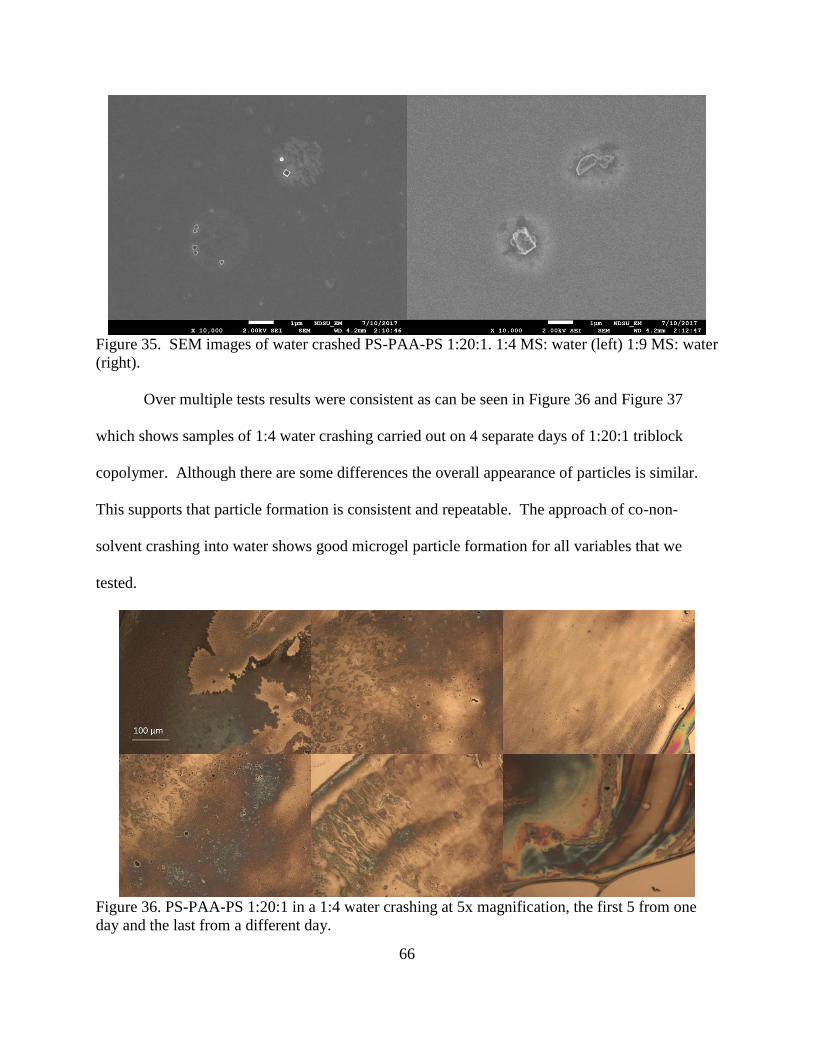
66
Figure 35. SEM images of water crashed PS-PAA-PS 1:20:1. 1:4 MS: water (left) 1:9 MS: water
(right).
Over multiple tests results were consistent as can be seen in Figure 36 and Figure 37
which shows samples of 1:4 water crashing carried out on 4 separate days of 1:20:1 triblock
copolymer. Although there are some differences the overall appearance of particles is similar.
This supports that particle formation is consistent and repeatable. The approach of co-non-
solvent crashing into water shows good microgel particle formation for all variables that we
tested.
Figure 36. PS-PAA-PS 1:20:1 in a 1:4 water crashing at 5x magnification, the first 5 from one
day and the last from a different day.
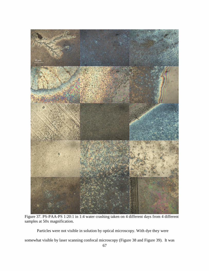
67
Figure 37. PS-PAA-PS 1:20:1 in 1:4 water crashing taken on 4 different days from 4 different
samples at 50x magnification.
Particles were not visible in solution by optical microscopy. With dye they were
somewhat visible by laser scanning confocal microscopy (Figure 38 and Figure 39). It was

68
challenging to discern what might have been particles and what might have been noise. There
was also a large amount of polymer that remained stuck to the Si wafer which leads to doubt that
an appreciable amount of polymer dissolved back into the water as particles. This sticking and
almost film formation is attributable to possible attraction between the particles and the substrate
or between the particles and themselves that keeps them from separating and dissolving into
solution.
Figure 38. Confocal imaging of PS-PAA-PS 1:50:1 crashed water in 1:4 ratio rehydrated at 10x
magnification. The left image is the channel showing the sample under visible light spectrum.
The right image is from the channel that imaged the sample under blue fluorescent laser.
Figure 39. Confocal imaging at 50x of PS-PAA-PS 1:50:1 ratio crashing in water 1:4 and
rehydrated, viewed at 50x with dyed particles visible under fluorescence channel on the right.
In order to better observe the particles if they do return to solution index mismatched
microscopy was carried out on an undyed sample. DIC index mismatching microscopy as in
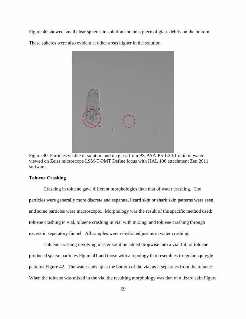
69
Figure 40 showed small clear spheres in solution and on a piece of glass debris on the bottom.
These spheres were also evident at other areas higher in the solution.
Figure 40. Particles visible in solution and on glass from PS-PAA-PS 1:20:1 ratio in water
viewed on Zeiss microscope LSM-T-PMT Define focus with HAL 100 attachment Zen 2011
software.
Toluene Crashing
Crashing in toluene gave different morphologies than that of water crashing. The
particles were generally more discrete and separate, lizard skin or shark skin patterns were seen,
and some particles were macroscopic. Morphology was the result of the specific method used:
toluene crashing in vial, toluene crashing in vial with mixing, and toluene crashing through
excess in seperatory funnel. All samples were rehydrated just as in water crashing.
Toluene crashing involving master solution added dropwise into a vial full of toluene
produced sparse particles Figure 41 and those with a topology that resembles irregular squiggle
patterns Figure 42. The water ends up at the bottom of the vial as it separates from the toluene.
When the toluene was mixed in the vial the resulting morphology was that of a lizard skin Figure

70
43, enhanced by heating Figure 44, or that of egg shaped particles depending on the polymer
length 1:50:1 resulted in lizard skin morphology while 1:20:1 resulted in egg shapes.
Figure 41. PS-PAA-PS 1:50:1 added dropwise to ~20mL of toluene at 50x magnification.
Figure 42. PS-PAA-PS 1:50:1 added dropwise to ~20mL of toluene at 50x magnification
concentrated a) dried with heater b) through f) were dried in air.
Figure 43. PS-PAA-PA 1:50:1 mixed in excess toluene for 24 hours allowed to dry in air and
rehydrated.
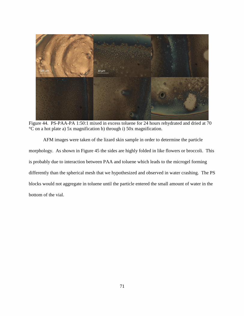
71
Figure 44. PS-PAA-PA 1:50:1 mixed in excess toluene for 24 hours rehydrated and dried at 70
°C on a hot plate a) 5x magnification b) through i) 50x magnification.
AFM images were taken of the lizard skin sample in order to determine the particle
morphology. As shown in Figure 45 the sides are highly folded in like flowers or broccoli. This
is probably due to interaction between PAA and toluene which leads to the microgel forming
differently than the spherical mesh that we hypothesized and observed in water crashing. The PS
blocks would not aggregate in toluene until the particle entered the small amount of water in the
bottom of the vial.

72
Figure 45. PS-PAA-PS 1:50:1 mixed in toluene and heat dried. AFM image scan size 10000 nm
x 10000 nm of height range ~20-50 nm.
The egg shaped particles were formed in toluene crashing for the shorter polymer 1:20:1.
The particles are so large that they are visible at low magnification as can be seen in Figure 46.
At higher magnifications all three of the above mentioned types are present, distinct particles,
lizard skins/ blue marble patterns, and egg like particles with center and surrounding haloes,
Figure 47. This method bares further investigation for particle morphology.
Figure 46: PS-PAA-PS 1:20:1 mixed in toluene for 24 hours at 5x magnification.
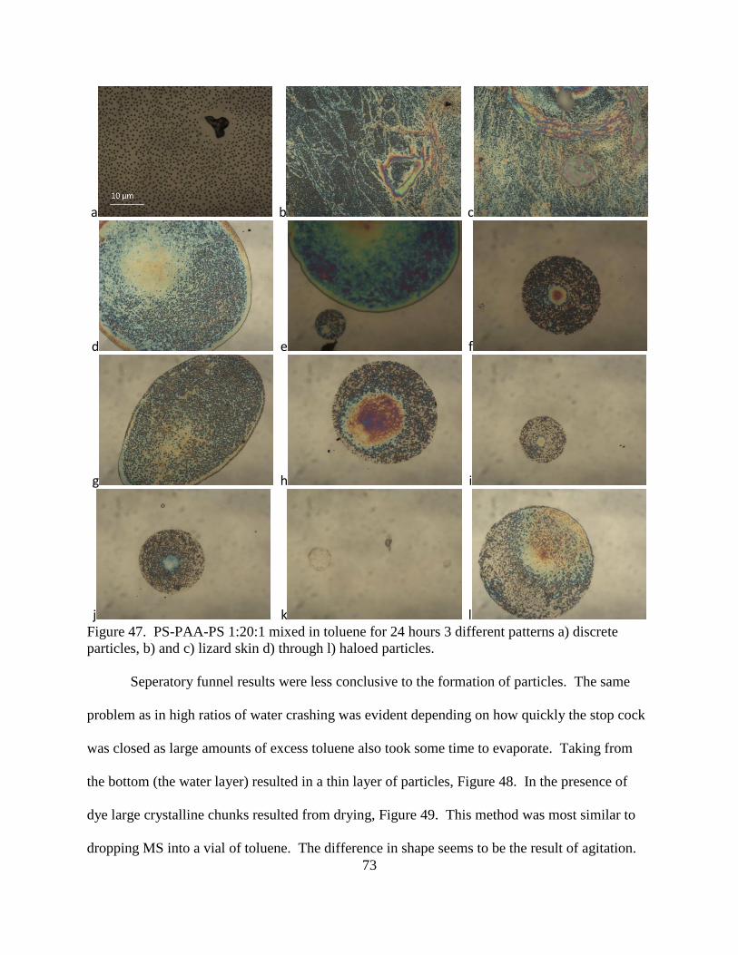
73
a b c
d e f
g h i
j k l Figure 47. PS-PAA-PS 1:20:1 mixed in toluene for 24 hours 3 different patterns a) discrete
particles, b) and c) lizard skin d) through l) haloed particles.
Seperatory funnel results were less conclusive to the formation of particles. The same
problem as in high ratios of water crashing was evident depending on how quickly the stop cock
was closed as large amounts of excess toluene also took some time to evaporate. Taking from
the bottom (the water layer) resulted in a thin layer of particles, Figure 48. In the presence of
dye large crystalline chunks resulted from drying, Figure 49. This method was most similar to
dropping MS into a vial of toluene. The difference in shape seems to be the result of agitation.
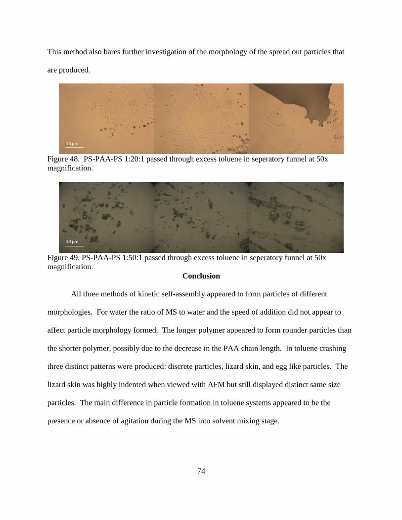
74
This method also bares further investigation of the morphology of the spread out particles that
are produced.
Figure 48. PS-PAA-PS 1:20:1 passed through excess toluene in seperatory funnel at 50x
magnification.
Figure 49. PS-PAA-PS 1:50:1 passed through excess toluene in seperatory funnel at 50x
magnification.
Conclusion
All three methods of kinetic self-assembly appeared to form particles of different
morphologies. For water the ratio of MS to water and the speed of addition did not appear to
affect particle morphology formed. The longer polymer appeared to form rounder particles than
the shorter polymer, possibly due to the decrease in the PAA chain length. In toluene crashing
three distinct patterns were produced: discrete particles, lizard skin, and egg like particles. The
lizard skin was highly indented when viewed with AFM but still displayed distinct same size
particles. The main difference in particle formation in toluene systems appeared to be the
presence or absence of agitation during the MS into solvent mixing stage.
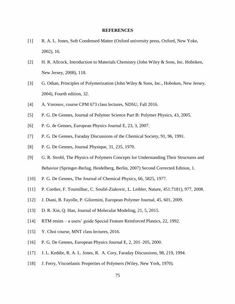
75
REFERENCES
[1] R. A. L. Jones, Soft Condensed Matter (Oxford university press, Oxford, New Yoke,
2002), 16.
[2] H. R. Allcock, Introduction to Materials Chemistry (John Wiley & Sons, Inc. Hoboken,
New Jersey, 2008), 118.
[3] G. Odian, Principles of Polymerization (John Wiley & Sons, Inc., Hoboken, New Jersey,
2004), Fourth edition, 32.
[4] A. Voronov, course CPM 673 class lectures, NDSU, Fall 2016.
[5] P. G. De Gennes, Journal of Polymer Science Part B: Polymer Physics, 43, 2005.
[6] P. G. de Gennes, European Physics Journal E, 23, 3, 2007.
[7] P. G. De Gennes, Faraday Discussions of the Chemical Society, 91, 96, 1991.
[8] P. G. De Gennes, Journal Physique, 31, 235, 1970.
[9] G. R. Strobl, The Physics of Polymers Concepts for Understanding Their Structures and
Behavior (Springer-Berlag, Heidelberg, Berlin, 2007) Second Corrected Edition, 1.
[10] P. G. De Gennes, The Journal of Chemical Physics, 66, 5825, 1977.
[11] P. Cordier, F. Tournilhac, C. Soulié-Ziakovic, L. Leibler, Nature, 451:7181), 977, 2008.
[12] J. Diani, B. Fayolle, P. Gilormini, European Polymer Journal, 45, 601, 2009.
[13] D. R. Xin, Q. Han, Journal of Molecular Modeling, 21, 5, 2015.
[14] RTM resins – a users’ guide Special Feature Reinforced Plastics, 22, 1992.
[15] Y. Choi course, MNT class lectures, 2016.
[16] P. G. De Gennes, European Physics Journal E, 2, 201–205, 2000.
[17] J. L. Keddie, R. A. L. Jones, R. A. Cory, Faraday Discussions, 98, 219, 1994.
[18] J. Ferry, Viscoelastic Properties of Polymers (Wiley, New York, 1970).
76
[19] O. A. Saleh, The Journal of Chemical Physics, 142, 194902, 2015.
[20] T. Annable, R. Buscall, R. Ettelaie, D. Whittlestone, Journal of Rheology, 37, 695, 1993.
[21] H. G. Allen, Analysis and Design of Structured Sandwich Panels, (Pergamon Press, New
York, NY, 1969) 178.
[22] Y. Ebata, A. B. Croll, A. J. Crosby, Soft Matter, 8, 9086, 2012.
[23] E. J. Kramer, Journal Advanced Polymer Science, 53, 1, 1983.
[24] C. Maestrini, E. J. Kramer, Polymer, 32:4, 1991.
[25] R. Tang, H. Huang, H. Tu, H. Liang, M. Liang, Z. Song, Y. Xu, H. Jiang, H. Yu, Applied
Physics Letters 104, 083501, 2014.
[26] Y. Zhang, Y. Huang , J. A. Rogers, Current Opinion in Solid State and Materials Science,
19, 190, 2015.
[27] M. Hasanzadeh , N. Shadjou, Materials Science and Engineering C, 61, 979, 2016.
[28] J. H. Cho, M. D. Keung, N. Verellen, L. Lagae, V. V. Moshchalkov, P. VanDorpe, D. H.
Gracias, Small, 7, 1943, 2011.
[29] H. Liu, H. Qing, Z. Lia, Y. L. Hana, M. Lina, H. Yang, A. Lie, T. J. Lub, F. Lib, F. Xu .
Materials Science and Engineering Review, 112, 1, 2017.
[30] R. A. Karnik, A. Löchtefeld, M. Subramanian, S. Bødker , S. Brewster , Morphees:
toward high “shape resolution” in self-actuated flexible mobile devices, Proc SIGCHI
Conference on Human Factors in Computing (Syst. Paris, France: ACM Press, 2013),
593.
[31] E. Mark, Automation in Construction, 22, 2, 2012.
[32] C. Liu, Y. Shi, Aerospace Science Technology, 53, 267, 2016.
[33] Q. Tao, C. Wang, Z. Xue, Z. Xie, H. Tan, Acta Astronaut, 128, 551, 2016.
77
[34] Y. Liu, J. Genzer, M. D. Dickey, Progress in Polymer Science, 52, 79, 2016.
[35] W. M. Huang, H. B. Lu, Y. Zhao , Z. Ding , C. C. Wang, J. L. Zhang , L. Sun , J. Fu, X.
Y. Gao, Materials and Design, 59, 176, 2014.
[36] L. Lia, W. Lia, H. Yanga, C. Maa, J. Yua, M. Yana, X. Song, Electrochimica Acta, 120,
102, 2014.
[37] D. Akinwande, C. J. Brennan, J. S. Bunch, P. Egberts, J. R. Felts, H. Gao, R. Huang, J. S.
Kim, T. Li, Y. Li, K. M. Liecht, N. Lu, H. S. Park, E. J. Reed, P. Wang, B. I. Yakobson,
T. Zhang, Y. W. Zhang, Y. Zhou, Y. Zhu, Extreme Mechanics Letters, 13, 42, 2017.
[38] J. R. Allensworth, Y. Liu, H. Braun, J. Genzer, M. D. Dickey, Polymer, 55:23, 5847,
2014.
[39] C. Lauff, T. W. Simpson, M. Frecker , Z. Ounaies, S. Ahmed, P. von Lockette, R.
Strzelec, R. Sheridan, J. M. Lien, ASME, 1, 2014.
[40] E. A. Peraza-Hernandez, D. J. Hartl, R. J. Malak Jr, D. C. Lagoudas, Smart Materials and
Structures, 23, 94001, 2014.
[41] S. Rohmer, et al. Geometric and topological modelling of 3d crumpled structures in: DS
75-4: Proceedings of the 19th International Conference on Engineering Design
(ICED13), Design for Harmonies, 4: Product, Service and Systems Design, (Seoul Seoul,
Korea, 2013), 4.
[42] J. L. Miller, Physics Today, 64:10, 15, 2011.
[43] L. Bevilacqua, Applied Mathematical Modelling, 28:6, 547, 2004.
[44] T. A. Witten, Reviews of Modern Physics, 79, 643, 2007.
[45] T. A. Witten, S. R. Nagel, Physical Review Letters, 88, 076101, 2002.
78
[46] J. Na, A. Evans, J. Bae, M. Chiappelli, C. Santangelo, R. Lang, T. Hull, R. Hayward,
Advanced Materials, 27, 79, 2015.
[47] Z. Wei, Z. Guo, L. Dudte, H. Liang, L. Mahadevan, Physical Review Letters, 110,
215501, 2013.
[48] T. G. Leong, A. M. Zarafshar, D. H. Gracias, Small, 6, 792, 2010.
[49] E. A. Peraza Hernandez, S. Hu, H. W. Kung, D. Hartl, E. Akleman, Computers &
Graphics, 37, 730, 2013.
[50] L. Mahadevan, S. Rica, Science, 307, 5716, 1740, 2005.
[51] F. Lechenault, B. Thiria, M. Abba-Bedia, Physical Review Letters, 112, 244301, 2014.
[52] W. J. Arora , H. I. Smith , G. Barbastathis, Microelectronic Engineering, 84, 1454, 2007.
[53] J. Caia,, Z. Ren, Y. Ding, X. Deng, Y. Xu, J. Fenge, Aerospace Science and Technology,
67, 343, 2017.
[54] A. Chiche, C. M. Stafford, J. T. Cabral, Soft Matter, 4, 2360, 2008.
[55] K. Efimenko, M. Rackaitis, E. Manias, A. Vaziri, L. Mahadevan, J. Genzer, Nature
Materials, 4, 293, 2005.
[56] F. Schneider, T. Fellner, J. Wilde, U. Wallrabe, Journal of Micromechanics and
Microengineering, 18, 065008, 2008.
[57] J. Mark, Polymer Data Handbook (Oxford Univ. Press, New York, 1999).
[58] I. D. Johnston, D. K. McCluskey, C. K. L. Tan, M. C. Tracey, Journal of Micromechanics
and Microengineering, 24, 035017, 2014.
[59] Dialectric Corporation, Retrieved December 12, 2017,
http://www.dielectriccorp.com/downloads/thermoplastics/lexan.pdf.
[60] Bekele J. Gurmessa and Andrew B. Croll, Physical Review Letters, 110, 07430 (2013).

79
[61] Boedeker Plastics, Inc., Shiner, Texas, USA, Retrieved December 12, 2017,
www.boedeker.com.
[62] The Engineering Toolbox, Retrieved December 12, 2017,
https://www.engineeringtoolbox.com/polymer-properties-d_1222.html.
[63] Matbase, Retrieved December 12, 2017, https://www.matbase.com/.
[64] X. Li, H. A. Hristov, A. F. Yee, Polymer, 36:4, 759, 1995.
[65] Gallina USA, Retrieved December 12, 2017, http://gallinausa.com/.
[66] C. Singer, E. J. Holmgard, A. R. Hall (eds), A History of Technology, (Oxford
University Press, New York, 1954).
[67] A. M. Abd, El-Khalek, Materials Science and Engineering: A, 500:1–2, 176, 2009.
[68] R. A. L. Jones, Soft Condensed Matter (Oxford university press, Oxford, New Yoke,
2002), 16.
[69] J. E. Pye, K. A. Rohald, E. A. Baker, C. B. Roth, Macromolecules, 43, 8296, 2010.
[70] K. Paeng, S. F. Swallen, M. D. Ediger, Journal of the American Chemical Society,
133:22, 8444, 2011.
[71] W. M. Lai, D. Rubin, E. Krempl, Introduction to Continuum Mechanics (Pergamon Press
Inc., Elmsford, New York, 1974) 239.
[72] L.D. Landau, E. M. Lifshitz. Course of Theoretical Physics Volume 7 Theory of
Elasticity (Pergamon Press, Elmsford, New York, 1986) Third Edition, 1.
[73] J. J. O’Dwyer, College Physics (Wadsworth Publishing Company, Belmont, California,
1981), 183.
[74] R. Lakes, Science, 235, 1987.
[75] A. Siber, H. Buljan, Physical Review E., 83, 067601, 2011.
80
[76] Croll group, private communications.
[77] W. G. Knauss, I. Emri, H. Lu, Mechanics of Polymers, 2006
[78] M. VanLandingham, P. Drzal, C. White. MRS Proceedings, 841, 2004.
[79] M. VanLandingham, N. K. Chang, P. L. Drzal, C. C. White, S. H. Chang, Polymer
Science, 43:14, 1794, 2005.
[80] N. N. Peschanskaya, P. N. Yakushev, V. M. Egorov, V. A. Bershtein, L. Bokobza,
Physics of the Solid State, 44:9, 1684, 2002.
[81] M. D. Shelby, G. L. Wilkes, Polymer, 39:26, 6767, 1998.
[82] P. A. O’Connell, S. A. Hutcheson, G. B. McKenna, Polymer Science, 46:18, 1952, 2008.
[83] H. Bodiguel, C. Fretigny, Macromolecules, 40:20, 7291, 2007.
[84] E. Cerda, S. Chaieb, F. Melo, L. Mahadevan, Nature, 401, 1999.
[85] S. Komura, K. Tamura, T. Kato, European Physical Journal E, 18, 343, 2005.
[86] T. Mora, A. Boudaoud, Europhysics Letters, 5:1, 41, 2002.
[87] A. E. H. Love, A Treatise on the Mathematical Theory of Elasticity (Dover, New York,
1944).
[88] T. Liang, T. A. Witten, Physical Review E 71, 016612, 2005.
[89] B. R. Saunders, B. Vincent, Advances in Colloid and Interface Science, 80, 1, 1999.
[90] G. E. Morris, B. Vincent, M. J. Snowden, Journal of Colloid Interface Science, 190, 198,
1997.
[91] A. Lyon, A. Fernandez-Nieves, Annual Review Physical Chemistry, 63,25, 2012.
[92] D. E. Discher, A. Eisenberg, Science, 2979, 967, 2002.
[93] R. H. Pelton , Adv. Colloid Interface Science, 85, 1, 2000.
81
[94] C. de las Heras Alarco´n, S. Pennadam, C. Alexander, Chemical Society Review, 34,
276, 2005.
[95] J. Mattsson, H. M. Wyss, A. Fernandez-Nieves, K. Miyazaki, Z. Hu, Nature, 462, 83,
2009.
[96] D. J. Pochan, J. Zhu, K. Zhang, K. L. Wooley, C. Miesch, T. Emrick, Soft Matter, 7,
2500, 2011.
[97] W. O. Baker, Industrial & Engineering Chemistry, 41, 511, 1949.
[98] R. A. L. Jones, Soft Condensed Matter (Oxford university press, Oxford, New Yoke,
2002), 16.
[99] T. Tanaka, D. J. Fillmore, Journal Chemical Physics, 70, 1214, 1979.
[100] C. Pichot, Current Opinion in Colloid & Interface Science, 9, 213, 2004.
[101] R. Messing, A. M. Schmidt, Polymer Chemistry, 2, 18, 2011.
[102] G. R. Hendrickson, L. A. Lyon, Angewandte Chemie International Edition in England,
49, 2193, 2010.
[103] P. Bouillot, B. Vincent, Colloid Polymer Science, 278, 74, 2000.
[104] K. Kita-Tokarczyk, J. Grumelard, T. Haefele, W. MeierBlock, Polymer, 46, 3540, 2005.
[105] L. A. Lyon, J. D. Debord, S. B. Debord, C. D. Jones, J. G. McGrath, M. J. Serpe, Journal
Physical Chemistry B, 108, 19099, 2004.
[106] K. S. Soni, S. S. Desale, T. K. Bronich, Journal of Controlled Release, 240, 109, 2016.
[107] Z. B. Hu, X. H. Lu, J. Gao, Advanced Materials, 13, 1708, 2001.
[108] J. D. Debord, L. A. Lyon, Journal Physical Chemistry B, 104, 6327, 2000.
[109] P. Pieranski, Contemporary Physics, 24, 25, 1983.

82
[110] M. Huiru, G. Jianguo, Y. Runzhang, Joumal of Wuhan University of Technology -
Material Science Education, 40:4, 43, 2005.
[111] H. M. Princen, Journal Colloid Interface Science, 91, 160, 1983.
[112] T. G. Mason, J. Bibette, D. A. Weitz D.A., Physical Review Letters, 1995.
[113] M. Cloitre, R. Borrega, L. Leibler, Physical Review Letters, 85, 4819, 2051, 2002.
[114] M. Cloitre, R. Borrega, F. Monti, L. Leibler, Physical Review Letters, 90, 068303, 2003.
[115] A. Einstein, Annals of Physics (Leipz.) 19, 371, 1906.
[116] M. E. Mackay, T. T. Dao, A. Tuteja, D. L. Ho, B. Van Horn, H. Kim, C. J. Hawker,
Nature Materials, 2, 2003.
[117] C. D. Jones, L. A. Lyon, Journal of American Chemical Society, 125, 460, 2003.
[118] C. D. Jones, M. J. Serpe, L. Schroeder, L. A. Lyon, Journal of American Chemical
Society, 125, 5292, 2003.
[119] A. N. St. John, L. A. Lyon, Journal Physical Chemistry B, 112, 11258, 2008.
[120] R. Vyhnalkova, A. H. E. Muller, A. Eisenberg, Langmuir, 30, 5031, 2014.
[121] R. H. Pelton, P. Chibante, Colloids and Surfaces, 120, 247, 1986.
[122] J. Clarke, B. J. Vincent, Journal of the Chemical Society, Faraday Transactions 1, 77,
1831, 1981.
[123] M. Antionietti, T. Pakula, W. Bremser, Macromolecules, 28, 4227, 1995.
[124] B. Neyret, B. Vincent, Polymer, 38, 6129, 1997.
[125] M. Frank, W. Burchard, Makromol. Chemical Rapid Communications, 12, 645, 1991.
[126] T. K. Bronich, P. A. Keifer, L. S. Shlyakhtenko, A. V. Kabanov, Journal of American
Chemical Society, 127, 8236, 2005.
[127] R. K. O'Reilly, C. J. Hawker, K. L. Wooley, Chemical Society Reviews, 35, 1068, 2006.
83
[128] C. Liu, M. A. Hillmyer, T. P. Lodge, Langmuir, 24, 12001, 2008.
[129] R. Zheng, G. Liu, X. Yan, Journal of American Chemical Society, 127, 15358, 2005.
[130] Z. H. Lu, G. J. Liu, F. T. Liu, Macromolecules, 34, 8814, 2001.
[131] X. S. Wang, G. Guerin, H. Wang, Y. Wang, I. Manners, M. A. Winnik, Science, 317,
644, 2007.
[132] W. McPhee, K. C. Tam, R. Pelton, Journal of Colloid and Interface Science, 4, 156,
1993.
[133] J. H. Holtz, S. A. Asher, Nature, 389, 829, 1997.
[134] Z. B. Li, E. Kesselman, Y. Talmon, M. A. Hillmyer, T. P. Lodge, Science, 306, 98,
2004.
[135] Z. B. Li, M. A. Hillmyer, T. P. Lodge, Nano Letters, 6, 1245, 2006.
[136] F. Schacher, A. Walther, A. H. E. Muller, Langmuir, 25, 10962, 2009.
[137] B. Fang, A. Walther, A. Wolf, Y. Xu, J. Yuan, A. H. E. Muller, Angewandte Chemie
International Edition, 48, 2877, 2009.
[138] H. Xu, F. Meng, Z. Zhong, Journal of Materials Chemistry, 19, 4183, 2009.
[139] L. Zhang, A. Eisenberg, Science, 268, 1728, 1995.
[140] P. Lim Soo, A. Eisenberg, Journal Polymer Science, Part B: Polymer Physics, 42, 923,
2004.
[141] G. H. Li, C. G. Cho, Korean Journal of Chemical Engineering, 25, 6, 1444, 2008.
[142] Y. N. Xue, Z. Z. Huang, J. T. Zhang, M. Liu, M. Zhang, S. W. Huang, R. X. Zhuo,
Polymer, 50:15, 3706, 2009.
[143] G. H. Li, P. P. Yang, Z. S. Gao, Y. Q. Zhu, Colloid Polymer Science, 290, 1825, 2012.
[144] L. Luo, A. Eisenberg, Langmuir, 17, 6804, 2001.
84
[145] L. Luo, A. Eisenberg, Journal of American Chemistry Society, 123, 1012, 2002.
[146] J. M. Weissman, H. B. Sunkara, A. S. Tse, S. A. Asher, Science, 274, 959, 1996.
[147] S. A. Rice, Chemical Physics Letters, 479, 1, 2009.
[148] J. Hostomskp, Z. Halasz, I. Liszi, J. Npvlt, Powder Technology, 49, 45, 1986.
[149] B. W. Longbottom, B. Somuncuog˘lu, J. J. Punter, S. Longbottom, S. A. F. Bon, Soft
Matter, 13, 4285, 2017.
[150] A. R. Denton, Q. Tang, The Journal of Chemical Physics, 145, 164901, 2016.
[151] D. P. Rozairo, A. B. Croll, Langmuir, 31, 1308, 2015.