Borrowing information across populations in estimating positive and

© 2011 Royal Statistical Society 0035–9254/11/60633

Appl. Statist. (2011)60, Part 5, pp. 633–653

Borrowing information across populations inestimating positive and negative predictive values

Ying Huang and Youyi Fong,

Fred Hutchinson Cancer Research Center, Seattle, USA

John Wei

University of Michigan, Ann Arbor, USA

and Ziding Feng

Fred Hutchinson Cancer Research Center, Seattle, USA

[Received April 2010. Final revision January 2011]

Summary. A marker’s capacity to predict the risk of a disease depends on the prevalence ofdisease in the target population and its accuracy of classification, i.e. its ability to discriminatediseased subjects from non-diseased subjects. The latter is often considered an intrinsic prop-erty of the marker; it is independent of disease prevalence and hence more likely to be similaracross populations than risk prediction measures. In this paper, we are interested in evaluatingthe population-specific performance of a risk prediction marker in terms of the positive predictivevalue PPV and negative predictive value NPV at given thresholds, when samples are availablefrom the target population as well as from another population. A default strategy is to estimatePPV and NPV using samples from the target population only. However, when the marker’saccuracy of classification as characterized by a specific point on the receiver operating char-acteristics curve is similar across populations, borrowing information across populations allowsincreased efficiency in estimating PPV and NPV. We develop estimators that optimally combineinformation across populations.We apply this methodology to a cross-sectional study where weevaluate PCA3 as a risk prediction marker for prostate cancer among subjects with or withouta previous negative biopsy.

Keywords: Biomarker; Classification; Negative predictive value; Positive predictive value;Sensitivity; Specificity

1. Introduction

The two most commonly used criteria for biomarker evaluation are the accuracy of classificationand risk prediction ability. The accuracy of classification, which is typically characterized by sen-sitivity, specificity and the receiver operating characteristics (ROC) curve (Pepe, 2003), measuresthe probability that a subject’s disease status is correctly identified on the basis of a biomarker.Risk prediction measures, in contrast, assess how well a marker can inform treatment optionson the basis of the predicted risk of disease. Among others, two measures that are often usedare the positive predictive value PPV and the negative predictive value NPV (Leisenring et al.,2000; Moskowitz and Pepe, 2004, 2006; Steinberg et al., 2008). It is well known that sensitivity,specificity and the ROC curve are intrinsic properties of a test whereas PPV and NPV depend

Address for correspondence: Ying Huang, Department of Vaccine and Infectious Disease and Public HealthSciences, Fred Hutchinson Cancer Research Center, 1100 Fairview Avenue North, Seattle, WA 98109, USA.E-mail: [email protected]

634 Y. Huang, Y. Fong, J. Wei and Z. Feng

on both the accuracy of classification and the external factor, i.e. the prevalence of the disease.However, there has been no method that utilizes this property to gain efficiency in estimatingPPVs and NPVs in populations of different prevalence of disease when data suggest commonintrinsic classification accuracy across populations, as in the application below that motivatedthis paper.

PCA3, a prostate-specific non-coding messenger ribonucleic acid that is overexpressed in pros-tate tumours, has been proposed as a risk prediction marker for prostate cancer. In a preliminarycross-sectional study, data were collected from 576 men immediately before their prostate biopsywhich was scheduled mainly because of elevated levels of prostate-specific antigen (Deras et al.,2006). About half of the subjects had a previous negative biopsy and the rest did not. Thedisease outcome is the prostate cancer status diagnosed by the biopsy. On the basis of thesedata, urologists are interested in evaluating PCA3’s risk prediction performance in terms ofPPV and NPV in the population of subjects who had had a previous biopsy and the popu-lation of subjects who had not had a previous biopsy. In particular the data suggested thatPPV at PCA3 value 60, which is approximately 0.75 in the initial biopsy population, could beused as a threshold for recommendation of prostate biopsy, and that NPV at PCA3 value 20,which is approximately 0.85 in the repeat biopsy population, to recommend against prostatebiopsy. These thresholds were recommended by study urologists on the basis that most prostatecancers are indolent and the fact that the prevalence of prostate cancer in the initial biopsypopulation is about 44%, and in the repeat biopsy population the prevalence is much lower ataround 27%. The difference in prevalence is due to the fact that larger tumours are likely to bedetected in the initial biopsy and that most prostate cancer patients were detected from theirinitial biopsy.

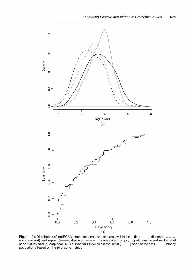
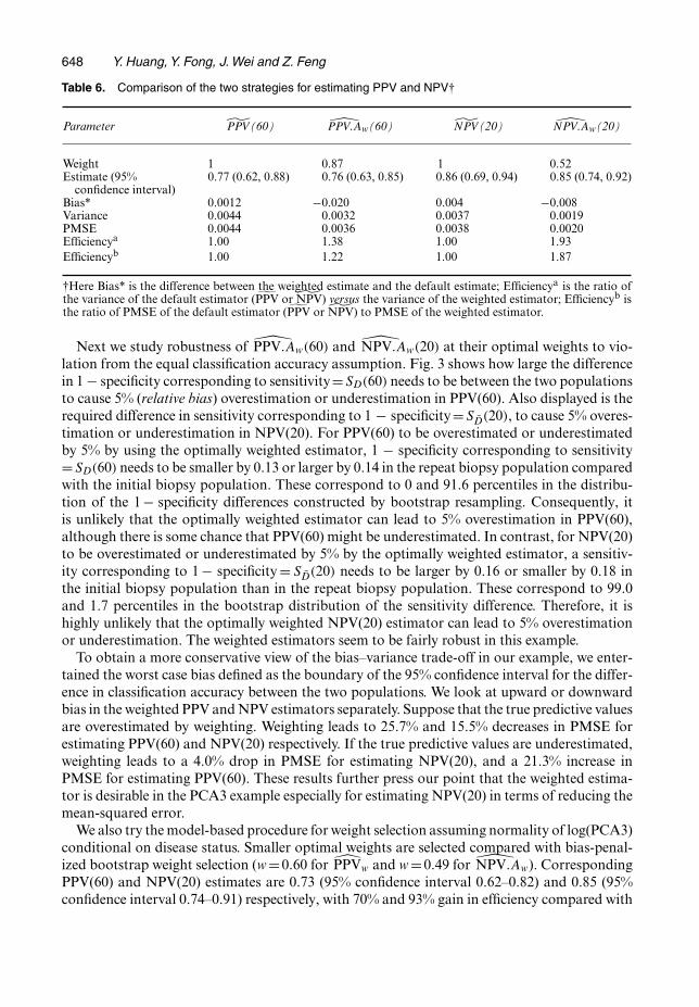
Fig. 1(a) shows the density functions of log(PCA3) conditional on disease status within theinitial and repeat biopsy populations, and Fig. 1(b) shows the empirical ROC curves in the twopopulations. Interestingly, although the distributions of PCA3 conditional on disease statusappear to differ between the two populations (for example, a Wilcoxon rank sum test applied tothe non-cancer groups has a p-value of 0.043), the two ROC curves appear similar to each other:the test of equal area under the curve has a p-value of 0.66. Scenarios where the ROC curve issimilar between different sources are not difficult to picture, considering the fact that the ROCcurve characterizes the comparison of diseased individuals and non-diseased individuals withrespect to their relative ranks rather than actual values. For example, it is common that assaysfrom different clinical centres could have different distributions due to many instrumental andspecimen handling factors, leading to some location–scale shifts of the test results across clinicalcentres, yet not changing the classification performance.

One major reason in favour of calculating PPV and NPV separately from each target popu-lation is that there are standard formulae for PPV and NPV for a single population as shownin Section 2, but there is no existing method for combining data across populations for estimat-ing PPV and NPV on the basis of the assumption of common classification accuracy, unlesswe use stronger assumptions, e.g. a location shift modelled by a population effect indicatorin the marker distributions conditional on disease status. The objective of the analysis that isdescribed in this paper is to develop a statistical method for estimating population-specific PPVand NPV by using the ROC curve as a bridge between populations when data strongly suggestthe same accuracy of classification across populations. This requires the assumption that relativeranks between diseased and non-diseased individuals are the same across populations. Makingassumptions based on rank is not uncommon in statistical literature owing to the increasedrobustness compared with making parametric assumptions on marker distribution. Examplesinclude the Friedman test (Friedman, 1937) and Quade test (Quade, 1979) in randomized block

Estimating Positive and Negative Predictive Values 635

0 2 4 6 8

0.0

0.1

0.2

0.3

0.4

log(PCA3)

Den

sity

(a)

0.0 0.2 0.4 0.6 0.8 1.0

0.0

0.2

0.4

0.6

0.8

1.0

1−Specificity

(b)

Sen

sitiv

ity

Fig. 1. (a) Distribution of log(PCA3) conditional on disease status within the initial ( , diseased; ,non-diseased) and repeat ( , diseased; , non-diseased) biopsy populations based on the pilotcohort study and (b) empirical ROC curves for PCA3 within the initial ( ) and the repeat ( ) biopsypopulations based on the pilot cohort study


design. The procedure that is proposed in this paper can be thought of as an expansion of thesenon-parametric methods to PPV or NPV estimation, rather than a simple hypothesis test ofequality of rank means. Combining information non-parametrically has a long history. Forexample, Mantel and Haenszel (1959) combined odds ratios across strata. In our example, it isdesirable to have a method that relies only on the similar rank distribution assumption and doesnot require explicit modelling, e.g. the location–scale shift effects on the marker distributionconditional on disease status.

The settings in which the procedure proposed will be useful assume that any ‘interaction’ effectof biomarker and population in terms of discriminating diseased from non-diseased individu-als is negligible, i.e. the difference in the marker’s discriminatory power between populationsis minimal. This assumption should always be checked. When the interaction is substantial,results from any of the above methods combining information across populations, includingthe method that is proposed in this paper, will be less interpretable and the estimation shouldbe done for each population. The main motivation of this paper is to provide a non-para-metric method for combining classification information across populations or strata when thecombined estimation is desired and justified.

Whereas cross-sectional samples and cohort samples are usually collected in the late phasesof biomarker studies, a case–control sampling design is most often used in the early phase ofbiomarker development (Pepe et al., 2001). In Section 2, we start by considering a case–controldesign and investigate cross-sectional and cohort designs later in Section 3. We present simu-lation studies in Section 4 and detailed analyses of the PCA3 example in Section 5. Finally weprovide concluding remarks in Section 6.

2. Methods in case–control design

Let D be a binary disease status and let Y be a continuous biomarker of interest. Suppose thatsamples are available from two populations: the target population where PPV and/or NPV areof interest, and another population that we call the auxiliary population. In the prostate cancerexample, the repeat biopsy population serves as the auxiliary population when we are interestedin estimating PPV and/or NPV in the initial biopsy population, and the initial biopsy populationwould serve as the auxiliary population when we are interested in estimating PPV and/or NPVin the repeat biopsy population. We use subscript D and D to indicate diseased and non-diseasedstatus, and superscript ‘Å’ to indicate the auxiliary population. Let Y , YD and YD be the markermeasured for a random subject, a case and a control respectively from the target population,and let YÅ, YÅ

D and YÅD

indicate the corresponding quantities in the auxiliary population. LetS.y/=P.Y >y/ denote the survival function for Y ; SD and SD denote the survival functions forYD and YD; SÅ

D and SÅD

denote the survival functions for YÅD and YÅ

D. Suppose that we apply a

binary classification rule to the target population such that, compared with a given threshold, asubject is classified as diseased if his marker value is greater than the threshold and non-diseasedotherwise. Then the ROC curve is the plot of true positive rate versus false positive rate for aseries of thresholds, and it can be expressed as ROC.t/ = SD{S−1

D.t/}. Similarly, let ROCÅ be

the corresponding ROC curve in the auxiliary population. We have ROCÅ.t/ = SÅD{SÅ−1

D.t/}.

Throughout this paper we assume that larger marker values are associated with higher risks ofdisease.

Next we explore methods for estimating PPV.y/=P.D=1|Y >y/. Results for NPV have beenomitted since they are easy to derive by exploiting the symmetry between the two: NPV.y/ =P.D=0|Y �y/ can be represented as PPV.−y/ when D is replaced by 1−D and Y replaced by−Y .


Let ρ indicate the prevalence of disease in the target population, which we assume initiallyto be known. By an application of Bayes’s theorem, PPV can be written as a function of ρ, SD

and SD:

PPV.y/= ρSD.y/

ρSD.y/+ .1−ρ/SD.y/: .1/

Writing y as S−1D

SD.y/ and using the definition of the ROC curve, PPV can be represented as afunction of ρ, SD and ROC{SD.y/}:

PPV.y/= ρSD{S−1D

SD.y/}ρSD{S−1

DSD.y/}+ .1−ρ/SD.y/

= ρROC{SD.y/}ρROC{SD.y/}+ .1−ρ/SD.y/

: .2/

Suppose that we sample nD cases {YD1, . . . , YDnD} and nD controls {YD1, . . . , YDnD} from the

target population and nÅD cases {YÅ

D1, . . . , YÅDn*

D} and nÅ

Dcontrols {YÅ

D1, . . . , YÅ

Dn*D} from the

auxiliary population. The default strategy for estimating PPV(y) is to estimate SD.y/ andSD.y/ empirically with SD.y/ = ΣnD

i=1.YDi > y/=nD and SD.y/ = ΣnDi=1.YDi > y/=nD and to en-

ter them into equation (1). Denote this estimator PPV.y/. This estimator is asymptoticallyequivalent to estimating SD.y/ with SD.y/ and estimating ROC{SD.y/} empirically with

˜ROC{SD.y/}=nD∑i=1

[YDi > SD

−1{SD.y/}]=nD,

and entering them into equation (2), since

˜ROC{SD.y/}�nD∑i=1

.YDi >y/=nD = SD.y/,

where the approximation is exact when y is one of the data points in the sample from the targetpopulation.

2.1. Estimator proposedIf, in addition, we have ROC.t/ = ROCÅ.t/ for t = SD.y/, i.e. the sensitivity corresponding tothe specificity 1 − SD.y/ is constant across the two populations, we can then estimate ROC(t)at t =SD.y/ by using samples from both populations. Let ˜ROC.t/ and ˜ROCÅ.t/ be the empiri-cal ROC from the target and auxiliary population respectively; the common ROC.t/ at t =SD.y/

can be estimated as a weighted average of the two ROCw.t/=w ˜ROC.t/+ .1−w/ ˜ROCÅ.t/, wheret = SD.y/ and w indicates the weight given to the empirical ROC estimate from the target pop-ulation.

Entering ROCw{SD.y/} and SD.y/ into equation (2), the weighted estimator for PPV.y/ is

PPVw.y/= ρ ROCw{SD.y/}ρ ROCw{SD.y/}+ .1−ρ/ SD.y/

,

where w =1 corresponds to estimating PPV by using samples from the target population only.Under the equal classification accuracy assumption, the asymptotic unbiasedness of the ROCand consequently that of the PPV estimators are invariant to the choice of w.

Let fD and fD be density functions of the marker for diseased and non-diseased individualsrespectively in the target population. In theorem 1 of Appendix A.1, we show that, under theassumption of equal sensitivity at specificity 1 − SD.y/, { PPVw.y/ − PPV.y/}√

nD is asymp-


totically normally distributed with zero mean and a variance term that is a function of w, ρ,SD.y/, SD.y/ and the density ratio fD.y/=fD.y/. Interestingly, since the asymptotic varianceof PPVw.y/ as shown in equation (4) in Appendix A.1 is a quadratic and convex function ofw, an optimal w that minimizes it can be uniquely determined, as presented in equation (5)of Appendix A.1. Moreover, observe that the asymptotic variance term (4) can be written asthe product of two terms: one free of w and the other free of ρ. Consequently the asymptoticrelative efficiency of any two estimators with specific weights is independent of the prevalenceof disease. In other words the optimal w is the same for all ρ. As shown in Appendix A.1, theoptimal w is always less than 1. It converges to 1 when nÅ

D=nD →0 or when nÅD

=nD →0. This isexpected intuitively since ˜ROCÅ is less precise than ˜ROC under these scenarios and we want toput more weight on the latter.

2.2. Alternative estimatorEarlier we proposed to estimate the specificity at a given threshold y empirically by using datafrom the target population, and to estimate the corresponding sensitivity by using data fromboth populations. Alternatively, we can start from the other direction, i.e. we could estimate thesensitivity at y empirically by using data from the target population and estimate the corres-ponding specificity by using data from both populations. We call this estimator

PPV:Aw.y/=ρ{SD.y/}=[ρ{SD.y/}+ .1−ρ/ ROC−1w { SD.y/}],

where

ROC−1w {SD.y/}=w

nD∑i=1

.YDi >y/=nD + .1−w/

n*D∑

i=1[YÅ

Di> SD

Å−1{SD.y/}]=nÅD

:

Asymptotic theory for this estimator and the optimal w for minimizing asymptotic varianceis established in theorems 3 and 4 of Appendix A.1. Again, the optimal w is always less than 1and independent of ρ. Interestingly, through simple algebra, it can be shown that the minimumasymptotic variances that are achievable by PPVw and PPV:Aw are equivalent. Consequently,as far as variance is concerned, asymptotically it does not matter whether we use sensitivity atthe given specificity as the bridge between populations or the other way around. We evaluatethe finite sample performance of the two estimators through simulation studies.

2.3. Imperfect disease prevalence estimateSo far we have assumed that the disease prevalence is known. Sometimes this is reasonable; forexample, if we obtain ρ from a population disease registry such as ‘Surveillance, epidemiology,and end results’ (http://seer.cancer.gov/), its value essentially can be treated as knownbecause of the large sample size that is involved. Alternatively a disease prevalence estimate ρmight be derived from a pilot cross-sectional study, like in our PCA3 application. Under such cir-cumstances, the asymptotic variance of PPVw.y/ and PPV:Aw computed in Sections 2.1 and 2.2could be easily modified to incorporate the variability in ρ as shown in theorem 5 of AppendixA.1. Suppose that we estimate sample prevalence from a pilot cohort study and apply it to theestimate of PPV based on the case–control sample; then the asymptotic variance of PPVw orPPV:Aw will equal their asymptotic variance given the ‘true’ ρ plus an extra term due to the esti-mation of ρ. From theorem 5, it can be easily seen that the optimal weights are invariant to theextra variability introduced and are the same as those in equations (5) and (7) in Appendix A.1where the disease prevalence is considered to be known. The efficiency of the optimal estimator


relative to the default estimator is expected to decrease as variability in the disease prevalenceestimator increases due to a dampening effect.

2.4. RobustnessThe estimators that were proposed in Sections 2.1 and 2.2 gain precision by assuming equal-ity between ROC{SD.y/} and ROCÅ{SD.y/} or between SÅ

DSÅ−1

D {SD.y/} and SD S−1D {SD.y/};

it is important to be aware of the magnitude of the bias in PPVw or PPV:Aw when thecorresponding assumptions are violated.

Let δ =ROCÅ.t/−ROC.t/ for t =SD.y/ and let

η =−[SÅD

SÅ−1D {SD.y/}−SD S−1

D {SD.y/}]:

As shown in theorems 6 and 7 of Appendix A.2, the asymptotic bias of PPVw can be repre-sented as a monotone increasing function of .1 − w/δ, and the asymptotic bias of PPV:Aw.y/

is a monotone increasing function of .1−w/η.In practice, researchers might be able to guess a suitable range for δ or η on the basis of

experience. Alternatively, an interval of δ or η that is consistent with the data can be derivedat, say, 95% confidence level. Then the asymptotic bias of the estimator proposed can be calcu-lated and combined with the reduction in variance to determine the ‘worst case’ effect on themean-squared error. Conversely, given a range of tolerable bias in PPVw.y/ or PPV:Aw.y/, wecan derive the corresponding tolerable range for δ or η.

2.5. Weight determination and variance estimationWe propose two approaches for determining the optimal weight w for computing PPVw orPPV:Aw and subsequently estimating the variance of the weighted estimators. The first approachis based on the closed form formula for w as presented in equations (5) and (7) in Appendix A.1for minimizing the asymptotic variance of the weighted estimators under equal classificationaccuracy conditions. Equations (6) and (7) involve a density ratio fD=fD which would be diffi-cult to estimate without making any parametric assumption about the marker distribution. Wethus propose to assume normality of Y in the target population conditional on disease statusand then to compute equations (6) and (7) on the basis of estimated distribution parameters. Inpractice, if we could transform data such that the normality assumption is not grossly violated,then we expect that the weight estimated by assuming normality would be a good approximationto the true entity. Since the choice of w will affect only efficiency of the estimator but not itsconsistency, robustness to deviations from normality is not a big issue for weight determination.Given selected w, one could apply asymptotic formulae (4) and (5) based on a normality assump-tion for estimation of variance. However, here deviation from normality could potentially biasthe variance estimation and invalidate the inference. Therefore, we recommend instead usingbootstrap resampling to estimate the variance of the weighted estimator after the optimal w hasbeen obtained through the asymptotic formula. The resampling scheme will be chosen to reflectsampling design.

Validity of the above approach for determining w relies on the equal classification accuracyassumption. In practice, a researcher’s choice of approaches for weight determination and var-iance estimation depends on the problem being investigated and reflects how strong one’s beliefis about the equal classification accuracy assumption and how heavily one is concerned aboutthe possible bias under the violation of this assumption. There are scenarios where the equalclassification accuracy is expected to hold where the approach that was described above is bestsuited. For example, consider a medical test performed at two different laboratories. It is quite


common to assume that the difference in laboratories leads to a location–scale shift in distri-bution of the test results but does not change the ranks of diseased versus non-diseased, andthus a common ROC curve exists. In other scenarios where the equal classification accuracyassumption is built largely on statistical tests rather than prior knowledge about the underlyingbiological mechanism, as in our PCA3 application, researchers might want to be conservativein terms of controlling possible bias while improving efficiency.

With an objective of maintaining a balance between bias and variance, here we propose asecond bootstrap-based approach for determining w. Specifically, we generate a bootstrap setbased on the observed data set and implement a grid search algorithm to examine a series ofcandidate w-values. In our simulation studies and application, a grid size of 0.01 is used. Foreach w, we estimate the bootstrap variance of the weighted estimators. At the same time, toaccount for possible deviation from the equal classification accuracy assumption, we also com-pute a ‘bias’ or penalty term as the difference between means of the weighted estimators overthe bootstrap distribution and the default estimator based on the original data. A weightedestimator with minimum ‘pseudo-mean-squared error’ PMSE, which is defined as the sum ofthe squared penalty and bootstrap variance, can then be selected out of all possible w-valuesand between PPVw and PPV:Aw. Here we use the same set of bootstrap samples for choosingw and for variance estimation. Doing so ignores the variability due to estimation of w. Con-ceptually, a more complicated bootstrap procedure could be implemented to account for thevariability in estimating w. However, it appears that, given a practical sample size, ignoring thecontribution to variability due to estimating w has minimal effect on the inference, as shown bythe satisfactory coverage of the weighted estimators in simulation studies. We thus adopt thissimpler bootstrap procedure instead of going for a more complicated procedure.

3. Estimation in cross-sectional or cohort design

The estimator that we developed in Section 2 for a case–control design is directly applicable toprospective sampling design. Consider the setting where n individuals in the target populationsare randomly sampled, among which nD subjects are diseased. Then the prevalence of diseasein the target population can be estimated by ρ=nD=n, whereas estimators SD.y/ and SD.y/ arecomputed in the same way as in Section 2. As demonstrated in Appendix A.3, here ρ is uncor-related with SD.y/ or SD.y/, considering the fact that SD.y/ and SD.y/ are estimated from theconditional distributions of marker given disease status, whereas ρ is a function only of diseasestatus data. Consequently, the asymptotic properties of PPVw.y/ and PPV:Aw are the same asthose presented in theorem 5.

4. Simulation

We conduct simulation studies to investigate the performance of the weighted estimators thatwere developed in earlier sections, using a case–control design. Assume that

YD ∼N.0, 1/,

YD ∼N.1, 1/,

YÅD

∼N.0:5, 1/,

YÅD ∼N.1:5, 1/:

⎫⎪⎪⎪⎬⎪⎪⎪⎭

.3/

Our goal is to estimate PPV.y/ in the target population. In the simulation, equal numbers ofsamples are obtained from the target population and from the auxiliary population, and within


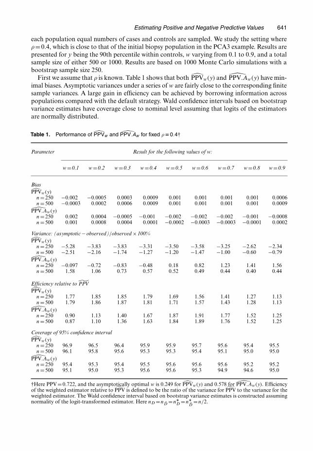
each population equal numbers of cases and controls are sampled. We study the setting whereρ=0:4, which is close to that of the initial biopsy population in the PCA3 example. Results arepresented for y being the 90th percentile within controls, w varying from 0.1 to 0.9, and a totalsample size of either 500 or 1000. Results are based on 1000 Monte Carlo simulations with abootstrap sample size 250.

First we assume that ρ is known. Table 1 shows that both PPVw.y/ and PPV:Aw.y/ have min-imal biases. Asymptotic variances under a series of w are fairly close to the corresponding finitesample variances. A large gain in efficiency can be achieved by borrowing information acrosspopulations compared with the default strategy. Wald confidence intervals based on bootstrapvariance estimates have coverage close to nominal level assuming that logits of the estimatorsare normally distributed.

Table 1. Performance of PPVw and PPV:Aw for fixed ρD0:4†

Parameter Result for the following values of w:

w =0.1 w =0.2 w =0.3 w =0.4 w =0.5 w =0.6 w =0.7 w =0.8 w =0.9

BiasPPVw.y/

n=250 −0.002 −0.0005 0.0003 0.0009 0.001 0.001 0.001 0.001 0.0006n=500 −0.0003 0.0002 0.0006 0.0009 0.001 0.001 0.001 0.001 0.0009

PPV:Aw.y/n=250 0.002 0.0004 −0.0005 −0.001 −0.002 −0.002 −0.002 −0.001 −0.0008n=500 0.001 0.0008 0.0004 0.0001 −0.0002 −0.0003 −0.0003 −0.0001 0.0002

Variance: (asymptotic−observed)=observed ×100%PPVw.y/

n=250 −5.28 −3.83 −3.83 −3.31 −3.50 −3.58 −3.25 −2.62 −2.34n=500 −2.51 −2.16 −1.74 −1.27 −1.20 −1.47 −1.00 −0.60 −0.79

PPV:Aw.y/n=250 −0.097 −0.72 −0.83 −0.48 0.18 0.82 1.23 1.41 1.56n=500 1.58 1.06 0.73 0.57 0.52 0.49 0.44 0.40 0.44

Efficiency relative to ˜PPVPPVw.y/

n=250 1.77 1.85 1.85 1.79 1.69 1.56 1.41 1.27 1.13n=500 1.79 1.86 1.87 1.81 1.71 1.57 1.43 1.28 1.13

PPV:Aw.y/n=250 0.90 1.13 1.40 1.67 1.87 1.91 1.77 1.52 1.25n=500 0.87 1.10 1.36 1.63 1.84 1.89 1.76 1.52 1.25

Coverage of 95% confidence intervalPPVw.y/

n=250 96.9 96.5 96.4 95.9 95.9 95.7 95.6 95.4 95.5n=500 96.1 95.8 95.6 95.3 95.3 95.4 95.1 95.0 95.0

PPV:Aw.y/n=250 95.4 95.3 95.4 95.5 95.6 95.6 95.6 95.2 95.2n=500 95.1 95.0 95.3 95.6 95.6 95.3 94.9 94.6 95.0

†Here PPV=0:722, and the asymptotically optimal w is 0.249 for PPVw.y/ and 0.578 for PPV:Aw.y/. Efficiencyof the weighted estimator relative to ˜PPV is defined to be the ratio of the variance for ˜PPV to the variance for theweighted estimator. The Wald confidence interval based on bootstrap variance estimates is constructed assumingnormality of the logit-transformed estimator. Here nD =nD =nÅ

D =nÅD

=n=2.


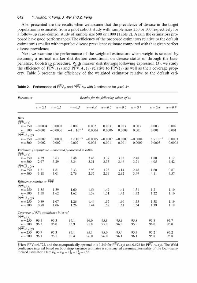
Also presented are the results when we assume that the prevalence of disease in the targetpopulation is estimated from a pilot cohort study with sample sizes 250 or 500 respectively fora follow-up case–control study of sample size 500 or 1000 (Table 2). Again the estimators pro-posed have good performances. The efficiency of the proposed estimators relative to the defaultestimator is smaller with imperfect disease prevalence estimate compared with that given perfectdisease prevalence.

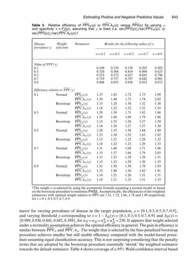
Next we examine the performance of the weighted estimators when weight is selected byassuming a normal marker distribution conditional on disease status or through the bias-penalized bootstrap procedure. With marker distributions following expression (3), we studythe efficiency of PPVw.y/ and PPV:Aw.y/ relative to PPV.y/ as well as their coverage prop-erty. Table 3 presents the efficiency of the weighted estimator relative to the default esti-

Table 2. Performance of PPVw and PPV:Aw with ρ estimated for ρD0:4†

Parameter Results for the following values of w:

w =0.1 w =0.2 w =0.3 w =0.4 w =0.5 w =0.6 w =0.7 w =0.8 w =0.9

BiasPPVw.y/

n=250 −0.0004 0.0008 0.002 0.002 0.003 0.003 0.003 0.003 0.002n=500 −0.001 −0.0006 −4×10−5 0.0004 0.0006 0.0008 0.001 0.001 0.001

PPV:Aw.y/

n=250 −0.002 0.0008 3×10−5 −0.0005 −0.0007 −0.0007 −0.0004 6×10−5 0.0003n=500 −0.002 −0.002 −0.002 −0.002 −0.001 −0.001 −0.0009 −0.0003 0.0003

Variance: (asymptotic−observed)=observed ×100%PPVw.y/

n=250 4.39 3.63 3.48 3.48 3.37 3.03 2.48 1.80 1.12n=500 −2.97 −3.29 −3.34 −3.31 −3.33 −3.46 −3.71 −4.05 −4.42

PPV:Aw.y/n=250 1.61 1.81 2.33 2.93 3.28 3.14 2.48 1.60 0.87n=500 −3.18 −3.01 −2.76 −2.57 −2.59 −2.92 −3.49 −4.11 −4.57

Efficiency relative to ˜PPVPPVw.y/

n=250 1.55 1.59 1.60 1.56 1.49 1.41 1.31 1.21 1.10n=500 1.58 1.62 1.62 1.58 1.51 1.42 1.32 1.22 1.10

PPV:Aw.y/n=250 0.89 1.07 1.26 1.44 1.57 1.60 1.53 1.38 1.19n=500 0.88 1.06 1.26 1.44 1.58 1.61 1.54 1.39 1.19

Coverage of 95% confidence intervalPPVw.y/

n=250 96.5 96.3 96.1 96.0 95.8 95.9 95.8 95.8 95.7n=500 96.3 96.0 95.9 95.8 95.9 96.0 95.9 96.0 96.0

PPV:Aw.y/n=250 95.7 95.3 95.1 95.1 95.0 95.4 95.3 95.2 95.2n=500 96.1 96.1 96.4 96.0 96.0 96.1 96.1 95.8 95.8

†Here PPV=0:722, and the asymptotically optimal w is 0.249 for PPVw.y/ and 0.578 for PPV:Aw.y/. The Waldconfidence interval based on bootstrap variance estimates is constructed assuming normality of the logit-trans-formed estimator. Here nD =nD =nÅ

D =nÅD

=n=2.


Table 3. Relative efficiency of PPVw.y/ or PPV:Aw.y/ versus PPV.y/ for varying ρand specificity v D F ND.y/, assuming that ρ is fixed (i.e. var{PPV.y/}=var{PPVw.y/} orvar{PPV.y/}=var{ PPV:Aw.y/}†

Disease Weight Parameter Results for the following values of v:prevalence ρ selection

v=0.1 v=0.3 v=0.5 v=0.7 v=0.9

Value of PPV(y)0.1 0.109 0.129 0.158 0.202 0.3020.3 0.320 0.364 0.419 0.494 0.6250.5 0.523 0.572 0.627 0.695 0.7960.7 0.719 0.757 0.797 0.842 0.9010.9 0.908 0.923 0.938 0.953 0.972

Efficiency relative to ˜PPV (y)0.1 Normal PPVw.y/ 1.33 1.45 1.72 1.75 1.99

PPV:Aw.y/ 1.39 1.48 1.73 1.74 2.02Bootstrap PPVw.y/ 1.15 1.20 1.30 1.32 1.36

PPV:Aw.y/ 1.18 1.22 1.32 1.32 1.350.3 Normal PPVw.y/ 1.29 1.59 1.71 1.82 1.86








PPV:Aw.y/ 1.18 1.21 1.25 1.31 1.33

†The weight w is selected by using the asymptotic formula assuming a normal model or basedon the bootstrap procedure to minimize PMSE. Asymptotically, the efficiencies of the weightedestimators with optimal weight relative to ˜PPV are 1.31, 1.52, 1.66, 1.78 and 1.89 respectivelyfor v=0:1, 0:3, 0:5, 0:7, 0:9.

mator for varying prevalence of disease in the target population, ρ = {0:1, 0:3, 0:5, 0:7, 0:9},and varying threshold y corresponding to v = 1 − SD.y/ = {0:1, 0:3, 0:5, 0:7, 0:9} and SD.y/ ={0:989, 0:936, 0:841, 0:682, 0:389}, for nD =nD =nÅ

D =nÅD

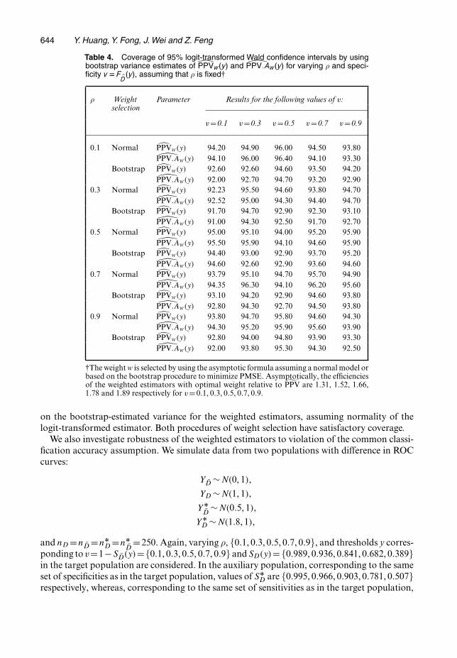
=250. It appears that weight selectedunder a normality assumption achieves the optimal efficiency in general. The gain in efficiency issimilar between PPVw and PPV:Aw. The weight that is selected by the bias-penalized bootstrapprocedure achieves smaller but still sizable efficiency compared with the model-based proce-dure assuming equal classification accuracy. This is not surprising considering that the penaltyterms that are adopted by the bootstrap procedure essentially ‘shrink’ the weighted estimatortowards the default estimator. Table 4 shows coverage of a 95% Wald confidence interval based


Table 4. Coverage of 95% logit-transformed Wald confidence intervals by usingbootstrap variance estimates of PPVw.y/ and PPV:Aw.y/ for varying ρ and speci-ficity v DF ND.y/, assuming that ρ is fixed†

ρ Weight Parameter Results for the following values of v:selection

v=0.1 v=0.3 v=0.5 v=0.7 v=0.9

0.1 Normal PPVw.y/ 94.20 94.90 96.00 94.50 93.80PPV:Aw.y/ 94.10 96.00 96.40 94.10 93.30

Bootstrap PPVw.y/ 92.60 92.60 94.60 93.50 94.20PPV:Aw.y/ 92.00 92.70 94.70 93.20 92.90









†The weight w is selected by using the asymptotic formula assuming a normal model orbased on the bootstrap procedure to minimize PMSE. Asymptotically, the efficienciesof the weighted estimators with optimal weight relative to ˜PPV are 1.31, 1.52, 1.66,1.78 and 1.89 respectively for v=0:1, 0:3, 0:5, 0:7, 0:9.

on the bootstrap-estimated variance for the weighted estimators, assuming normality of thelogit-transformed estimator. Both procedures of weight selection have satisfactory coverage.

We also investigate robustness of the weighted estimators to violation of the common classi-fication accuracy assumption. We simulate data from two populations with difference in ROCcurves:

YD ∼N.0, 1/,

YD ∼N.1, 1/,

YÅD

∼N.0:5, 1/,

YÅD ∼N.1:8, 1/,

and nD =nD =nÅD =nÅ

D=250. Again, varying ρ, {0:1, 0:3, 0:5, 0:7, 0:9}, and thresholds y corres-

ponding to v=1−SD.y/={0:1, 0:3, 0:5, 0:7, 0:9} and SD.y/= {0:989, 0:936, 0:841, 0:682, 0:389}in the target population are considered. In the auxiliary population, corresponding to the sameset of specificities as in the target population, values of SÅ

D are {0:995, 0:966, 0:903, 0:781, 0:507}respectively, whereas, corresponding to the same set of sensitivities as in the target population,


values of 1 − SÅD

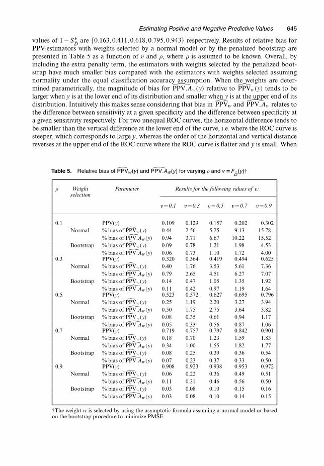
are {0:163, 0:411, 0:618, 0:795, 0:943} respectively. Results of relative bias forPPV-estimators with weights selected by a normal model or by the penalized bootstrap arepresented in Table 5 as a function of v and ρ, where ρ is assumed to be known. Overall, byincluding the extra penalty term, the estimators with weights selected by the penalized boot-strap have much smaller bias compared with the estimators with weights selected assumingnormality under the equal classification accuracy assumption. When the weights are deter-mined parametrically, the magnitude of bias for PPV:Aw.y/ relative to PPVw.y/ tends to belarger when y is at the lower end of its distribution and smaller when y is at the upper end of itsdistribution. Intuitively this makes sense considering that bias in PPVw and PPV:Aw relates tothe difference between sensitivity at a given specificity and the difference between specificity ata given sensitivity respectively. For two unequal ROC curves, the horizontal difference tends tobe smaller than the vertical difference at the lower end of the curve, i.e. where the ROC curve issteeper, which corresponds to large y, whereas the order of the horizontal and vertical distancereverses at the upper end of the ROC curve where the ROC curve is flatter and y is small. When

Table 5. Relative bias of PPVw.y/ and PPV:Aw.y/ for varying ρ and v DF ND.y/†

ρ Weight Parameter Results for the following values of v:selection

v=0.1 v=0.3 v=0.5 v=0.7 v=0.9

0.1 PPV(y) 0.109 0.129 0.157 0.202 0.302Normal % bias of PPVw.y/ 0.44 2.56 5.25 9.13 15.78

% bias of PPV:Aw.y/ 0.94 3.71 6.67 10.22 15.52Bootstrap % bias of PPVw.y/ 0.09 0.78 1.21 1.98 4.53

% bias of PPV:Aw.y/ 0.06 0.73 1.10 1.72 4.000.3 PPV(y) 0.320 0.364 0.419 0.494 0.625

Normal % bias of PPVw.y/ 0.40 1.76 3.53 5.61 7.36% bias of PPV:Aw.y/ 0.79 2.65 4.51 6.27 7.07

Bootstrap % bias of PPVw.y/ 0.14 0.47 1.05 1.35 1.92% bias of PPV:Aw.y/ 0.11 0.42 0.97 1.19 1.64



% bias of PPV:Aw.y/ 0.05 0.33 0.56 0.87 1.060.7 PPV(y) 0.719 0.757 0.797 0.842 0.901

Normal % bias of PPVw.y/ 0.18 0.70 1.23 1.59 1.83% bias of PPV:Aw.y/ 0.34 1.00 1.55 1.82 1.77

Bootstrap % bias of PPVw.y/ 0.08 0.25 0.39 0.36 0.54% bias of PPV:Aw.y/ 0.07 0.23 0.37 0.33 0.50



% bias of PPV:Aw.y/ 0.03 0.08 0.10 0.14 0.15

†The weight w is selected by using the asymptotic formula assuming a normal model or basedon the bootstrap procedure to minimize PMSE.


the bias-penalized bootstrap procedure is used for weight selection, the bias is similar betweenPPVw and PPV:Aw.

5. Application to PCA3 study

In the PCA3 study (Deras et al., 2006), information was collected for 267 subjects from theinitial biopsy population and another 269 different subjects from the repeat biopsy population.As mentioned in Section 1, researchers are interested in evaluating PCA3’s ability to identifyhigh risk subjects in the initial biopsy population and its ability to identify low risk subjects inthe repeat biopsy population. PPV(60) and NPV(20) were chosen as the measures to evaluate.

Define NPVw to be the weighted estimator for NPV by using specificity at a particular sen-sitivity as the bridge between populations and let NPV:Aw be the alternative estimator wheresensitivity at a particular specificity is used as the bridge. To evaluate the validity of assumptionsfor PPVw.60/, PPV:Aw.60/, NPVw.20/ and NPV:Aw.20/, tests are conducted using bootstrapvariance estimates for equivalence between the two populations with respect to

(a) sensitivity corresponding to 1− specificity=SD.60/,(b) specificity corresponding to sensitivity=SD.60/,(c) specificity corresponding to sensitivity=SD.20/ and(d) sensitivity corresponding to 1− specificity=SD.20/.

With respect to these four measures, point estimates in the initial and repeat biopsy populationsare

(a) {0:314, 0:236},(b) {0:081, 0:132},(c) {0:730, 0:764} and(d) {0:503, 0:487} respectively.

None of the test results are significant. The p-values are 0.433, 0.315, 0.665 and 0.864 respec-tively.

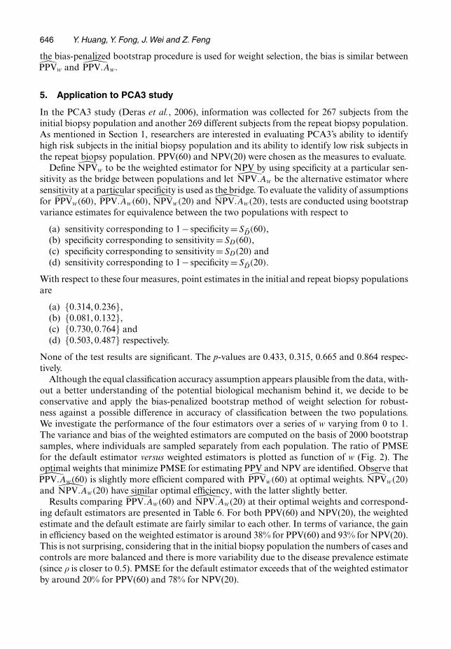
Although the equal classification accuracy assumption appears plausible from the data, with-out a better understanding of the potential biological mechanism behind it, we decide to beconservative and apply the bias-penalized bootstrap method of weight selection for robust-ness against a possible difference in accuracy of classification between the two populations.We investigate the performance of the four estimators over a series of w varying from 0 to 1.The variance and bias of the weighted estimators are computed on the basis of 2000 bootstrapsamples, where individuals are sampled separately from each population. The ratio of PMSEfor the default estimator versus weighted estimators is plotted as function of w (Fig. 2). Theoptimal weights that minimize PMSE for estimating PPV and NPV are identified. Observe thatPPV:Aw.60/ is slightly more efficient compared with PPVw.60/ at optimal weights. NPVw.20/

and NPV:Aw.20/ have similar optimal efficiency, with the latter slightly better.Results comparing PPV:Aw.60/ and NPV:Aw.20/ at their optimal weights and correspond-

ing default estimators are presented in Table 6. For both PPV(60) and NPV(20), the weightedestimate and the default estimate are fairly similar to each other. In terms of variance, the gainin efficiency based on the weighted estimator is around 38% for PPV(60) and 93% for NPV(20).This is not surprising, considering that in the initial biopsy population the numbers of cases andcontrols are more balanced and there is more variability due to the disease prevalence estimate(since ρ is closer to 0.5). PMSE for the default estimator exceeds that of the weighted estimatorby around 20% for PPV(60) and 78% for NPV(20).


0.0

0.2

0.4

0.6

0.8

1.0

1.2

w

PM

SE

Def

ault/

PM

SE

Wei

ghte

d

0.0 0.2 0.4 0.6 0.8 1.0

(a)

w(b)

0.0 0.2 0.4 0.6 0.8 1.0

0.0

0.5

1.0

1.5

2.0

PM

SE

Def

ault/

PM

SE

Wei

ghte

d

Fig. 2. Ratio of PMSE for the default estimator versus the weighted estimator of (a) PPV(60) ( , PPVw;, PPV:Aw) and (b) NPV(20) ( , NPVw; , NPV:Aw) as functions of weight


Table 6. Comparison of the two strategies for estimating PPV and NPV†

Parameter ˜PPV (60) PPV:Aw(60) ÑPV (20) NPV:Aw(20)

Weight 1 0.87 1 0.52Estimate (95% 0.77 (0.62, 0.88) 0.76 (0.63, 0.85) 0.86 (0.69, 0.94) 0.85 (0.74, 0.92)

confidence interval)Bias* 0.0012 −0.020 0.004 −0.008Variance 0.0044 0.0032 0.0037 0.0019PMSE 0.0044 0.0036 0.0038 0.0020Efficiencya 1.00 1.38 1.00 1.93Efficiencyb 1.00 1.22 1.00 1.87

†Here Bias* is the difference between the weighted estimate and the default estimate; Efficiencya is the ratio ofthe variance of the default estimator ( ˜PPV or ÑPV) versus the variance of the weighted estimator; Efficiencyb isthe ratio of PMSE of the default estimator ( ˜PPV or ÑPV) to PMSE of the weighted estimator.

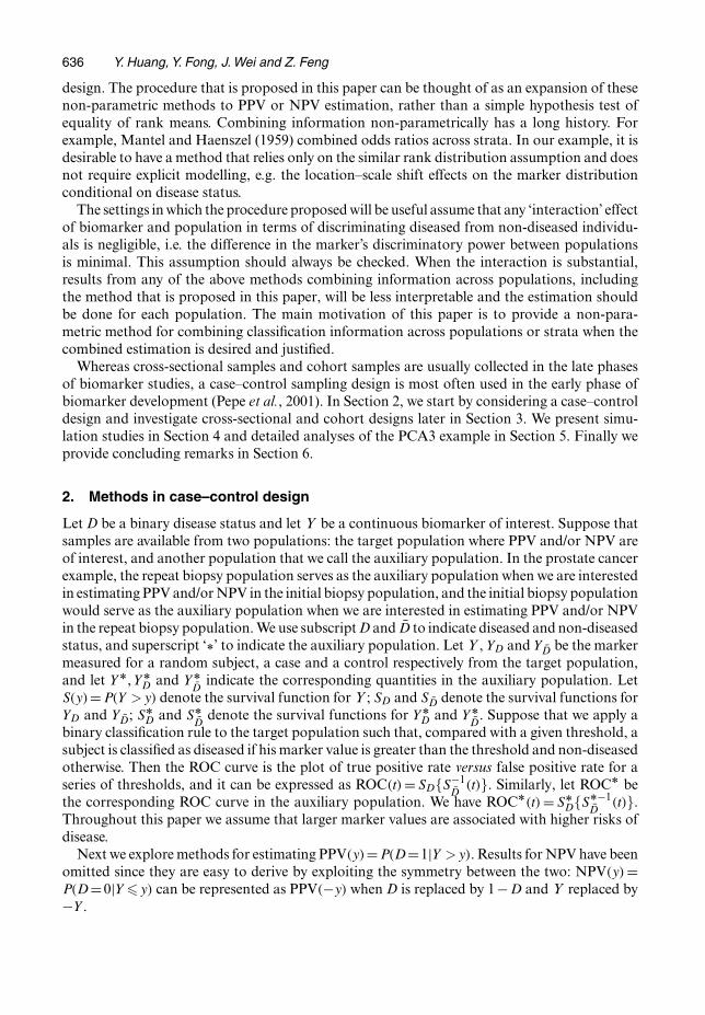
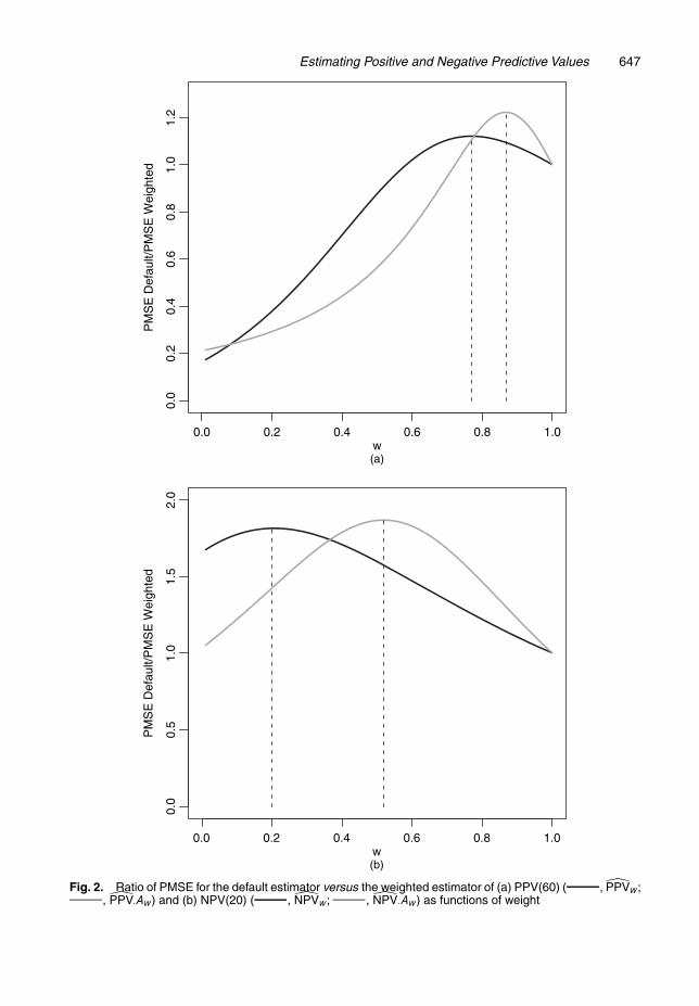
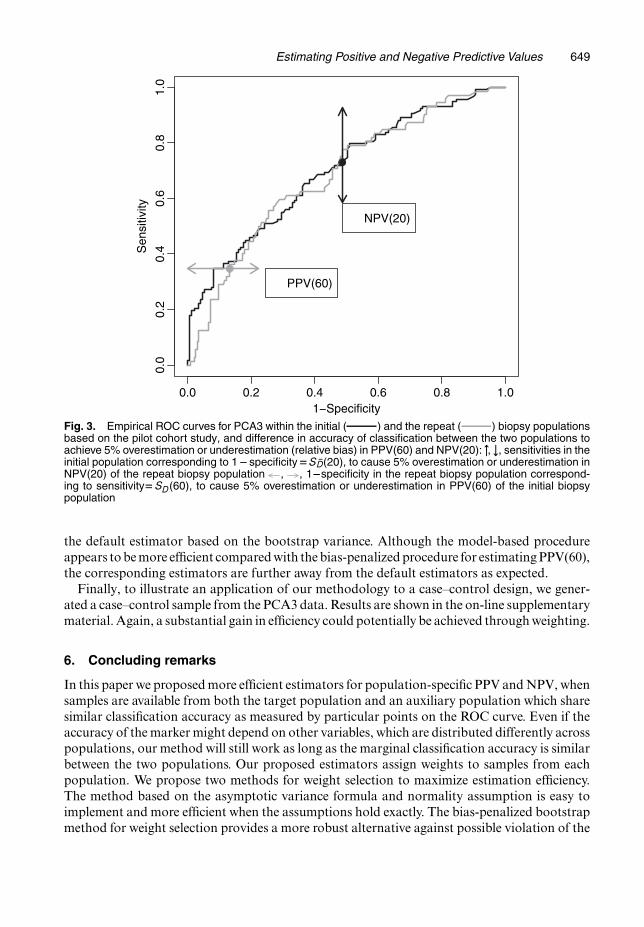
Next we study robustness of PPV:Aw.60/ and NPV:Aw.20/ at their optimal weights to vio-lation from the equal classification accuracy assumption. Fig. 3 shows how large the differencein 1 − specificity corresponding to sensitivity=SD.60/ needs to be between the two populationsto cause 5% (relative bias) overestimation or underestimation in PPV(60). Also displayed is therequired difference in sensitivity corresponding to 1 − specificity=SD.20/, to cause 5% overes-timation or underestimation in NPV(20). For PPV(60) to be overestimated or underestimatedby 5% by using the optimally weighted estimator, 1 − specificity corresponding to sensitivity=SD.60/ needs to be smaller by 0.13 or larger by 0.14 in the repeat biopsy population comparedwith the initial biopsy population. These correspond to 0 and 91.6 percentiles in the distribu-tion of the 1− specificity differences constructed by bootstrap resampling. Consequently, itis unlikely that the optimally weighted estimator can lead to 5% overestimation in PPV(60),although there is some chance that PPV(60) might be underestimated. In contrast, for NPV(20)to be overestimated or underestimated by 5% by the optimally weighted estimator, a sensitiv-ity corresponding to 1 − specificity = SD.20/ needs to be larger by 0.16 or smaller by 0.18 inthe initial biopsy population than in the repeat biopsy population. These correspond to 99.0and 1.7 percentiles in the bootstrap distribution of the sensitivity difference. Therefore, it ishighly unlikely that the optimally weighted NPV(20) estimator can lead to 5% overestimationor underestimation. The weighted estimators seem to be fairly robust in this example.

To obtain a more conservative view of the bias–variance trade-off in our example, we enter-tained the worst case bias defined as the boundary of the 95% confidence interval for the differ-ence in classification accuracy between the two populations. We look at upward or downwardbias in the weighted PPV and NPV estimators separately. Suppose that the true predictive valuesare overestimated by weighting. Weighting leads to 25.7% and 15.5% decreases in PMSE forestimating PPV(60) and NPV(20) respectively. If the true predictive values are underestimated,weighting leads to a 4.0% drop in PMSE for estimating NPV(20), and a 21.3% increase inPMSE for estimating PPV(60). These results further press our point that the weighted estima-tor is desirable in the PCA3 example especially for estimating NPV(20) in terms of reducing themean-squared error.

We also try the model-based procedure for weight selection assuming normality of log(PCA3)conditional on disease status. Smaller optimal weights are selected compared with bias-penal-ized bootstrap weight selection (w =0:60 for PPVw and w =0:49 for NPV:Aw). CorrespondingPPV(60) and NPV(20) estimates are 0.73 (95% confidence interval 0.62–0.82) and 0.85 (95%confidence interval 0.74–0.91) respectively, with 70% and 93% gain in efficiency compared with


0.0 0.2 0.4 0.6 0.8 1.0

0.0

0.2

0.4

0.6

0.8

1.0

1−Specificity

Sen

sitiv

ity

PPV(60)

NPV(20)

Fig. 3. Empirical ROC curves for PCA3 within the initial ( ) and the repeat ( ) biopsy populationsbased on the pilot cohort study, and difference in accuracy of classification between the two populations toachieve 5% overestimation or underestimation (relative bias) in PPV(60) and NPV(20): ", #, sensitivities in theinitial population corresponding to 1�specificityDS ND.20/, to cause 5% overestimation or underestimation inNPV(20) of the repeat biopsy population , , 1�specificity in the repeat biopsy population correspond-ing to sensitivityD SD.60/, to cause 5% overestimation or underestimation in PPV(60) of the initial biopsypopulation

the default estimator based on the bootstrap variance. Although the model-based procedureappears to be more efficient compared with the bias-penalized procedure for estimating PPV(60),the corresponding estimators are further away from the default estimators as expected.

Finally, to illustrate an application of our methodology to a case–control design, we gener-ated a case–control sample from the PCA3 data. Results are shown in the on-line supplementarymaterial. Again, a substantial gain in efficiency could potentially be achieved through weighting.

6. Concluding remarks

In this paper we proposed more efficient estimators for population-specific PPV and NPV, whensamples are available from both the target population and an auxiliary population which sharesimilar classification accuracy as measured by particular points on the ROC curve. Even if theaccuracy of the marker might depend on other variables, which are distributed differently acrosspopulations, our method will still work as long as the marginal classification accuracy is similarbetween the two populations. Our proposed estimators assign weights to samples from eachpopulation. We propose two methods for weight selection to maximize estimation efficiency.The method based on the asymptotic variance formula and normality assumption is easy toimplement and more efficient when the assumptions hold exactly. The bias-penalized bootstrapmethod for weight selection provides a more robust alternative against possible violation of the


common classification accuracy assumption, although it loses some efficiency relative to thecorrectly specified model-based procedure.

In theory, the common classification accuracy assumption holds in the following scenario.Suppose that cases and controls in the auxiliary population, after some monotone transfor-mation g, follow the same distributions as cases and controls in the target population; thenSÅ

D.YÅ

D/ = P.YÅD

� YÅD/ = P{g.YÅ

D/ � g.YÅ

D/}= P.YD � YD/ = SD.YD/, which implies the equiva-lence between the ROC curves. This holds because P{SD.YD/� t}=P{YD �S−1

D.t/}=ROC.t/,

i.e. ROC is the cumulative density function of SD.YD/, the ‘placement’ of YD among the controldistribution (Pepe and Cai, 2004). Here the population indicator is a confounder in evaluatingthe accuracy of classification of the marker; the threshold of marker value to achieve a givenspecificity is different across populations but the sensitivity corresponding to a given specificityremains the same (Janes and Pepe, 2010a,b). Our methods provide a way to adjust for the con-founding effect of population with a goal of estimating population-specific predictive values. Inpractice, whether the accuracy of classification of a biomarker is similar across populations canbe explored by using the data. And we can further conduct tests for equal classification accuracyas we did in the PCA3 example. This is analogous to a test of the interaction between a markerand covariate in a standard regression setting to rule out the possibility that the covariate (inour setting the population indicator) would affect the marker’s discriminatory performance. Weshould also work closely with scientists to decide whether a reasonable true difference in ROCcurves would lead to intolerable bias in PPV- and NPV-estimation.

Acknowledgements

The authors are grateful for support provided by National Cancer Institute grant CA86368.And we thank the Joint Editor, Associate Editor and referees for their helpful comments andsuggestions.

Appendix A

Proofs of all results that are not given explicitly in the text are available in the on-line supplementarymaterial.

A.1. Asymptotic variance of the weighted PPV-estimatorsHere we present asymptotic theory for the proposed estimator defined in Sections 2.1 and 2.2. We assumethat the following conditions hold:

(a) the distribution functions of YD, YD, YÅD and YÅ

Dare differentiable with density functions fD, fD,

fÅD and fÅ

Drespectively;

(b) as nD →∞, nD=nD →λ, nÅD

=nD →λ1 and nÅD=nD →λ2. This implies that .nÅ

D + nÅD

/=.nD + nD/ →.λ1 +λλ2/=.1+λ/, nD=.nD +nD/→λ=.1+λ/ and nÅ

D=.nÅD +nÅ

D/→λλ2=.λλ2 +λ1/, i.e. the ratio of

the sample sizes from the two populations converges to a constant, and the proportion of diseasedin each population converges to a population-specific constant.

Consistency of PPVw.y/ and PPV:Aw.y/ follows from the continuous mapping theorem.

Theorem 1.{ PPVw.y/−PPV.y/}√nD is asymptotically normally distributed with mean 0 and variance

Σw =A11VD.y/+A12fD.y/

fD.y/.1−w/VD.y/

+A22

[.1−w/2

(1+ 1

λ1

){fD.y/

fD.y/

}2

VD.y/+ 1λ

{w2 + .1−w/2 1

λ2

}VD.y/

], .4/

where VD.y/=SD.y/{1−SD.y/}, VD.y/=SD.y/{1−SD.y/},


A11 =[

ρ.1−ρ/

{ρSD.y/+ .1−ρ/SD.y/}2

]2

SD.y/2,

A12 =−2[

ρ.1−ρ/

{ρSD.y/+ .1−ρ/SD.y/}2

]2

SD.y/SD.y/,

A22 =[

ρ.1−ρ/

{ρSD.y/+ .1−ρ/SD.y/}2

]2

SD.y/2:

When w = 1, Σw reduces to A11VD.y/ + A22VD.y/=λ, which is the asymptotic variance of the defaultestimator PPV.y/.

Observe that Σw is a quadratic function of w, which is convex since A22 > 0. In addition, Σw can bewritten as the product of [ρ.1−ρ/={ρSD.y/+ .1−ρ/SD.y/}2]2 and another term that is free of ρ.

Theorem 2. Asymptotic variance of PPVw.y/ is minimized when

w =A12

fD.y/

fD.y/VD.y/+2A22

(1+ 1

λ1

){fD.y/

fD.y/

}2

VD.y/+2A221λ2

1λ

VD.y/

2A22

(1+ 1

λ1

){fD.y/

fD.y/

}2

VD.y/+2A221λ2

1λ

VD.y/+2A221λ

VD.y/

: .5/

Since A12 < 0, the optimal w is always less than 1.

Theorem 3.{ PPV:Aw.y/−PPV.y/}√nD is asymptotically normally distributed with mean 0 and variance

Σ:Aw =A11

[.1−w/2

(1+ 1

λ2

){fD.y/

fD.y/

}2 1λ

VD.y/+{

w2 + .1−w/2 1λ1

}VD.y/

],

+A12fD.y/

fD.y/.1−w/

1λ

VD.y/+A221λ

VD.y/: .6/

Theorem 4. Asymptotic variance of PPV:Aw.y/ is minimized when

w =A12

fD.y/

fD.y/

1λ

VD.y/+2A11

(1+ 1

λ2

){fD.y/

fD.y/

}2 1λ

VD.y/+2A111λ1

VD.y/

2A11

(1+ 1

λ2

){fD.y/

fD.y/

}2 1λ

VD.y/+2A111λ1

VD.y/+2A11VD.y/

: .7/

The optimal w is always less than 1.

Theorem 5. Suppose that we use sample prevalence ρ derived from a pilot cohort study with sample sizenc, such that var.ρ/=σ2=nc, and suppose that nc=nD → ξ as nD →∞. Then, compared with known ρ,the asymptotic variance of { PPVw.y/−PPV.y/}√

nD as nD →∞ increases by a term

σ2

ξ

SD.y/2 SD.y/2

{ρSD.y/+ .1−ρ/SD.y/}4:

The same applies to the asymptotic variance of PPV:Aw.y/.

A.2. Asymptotic bias of the weighted PPV-estimatorsTheorems 6 and 7 present the asymptotic bias of PPVw and PPV:Aw as a function of the difference insensitivity between the two populations with specificity fixed at 1−SD.y/ and the difference in specificitybetween the two populations with sensitivity fixed at SD.y/. The derivation is presented in the supplemen-tary material.


Theorem 6. Let δ =ROCÅ.t/−ROC.t/ for t =SD.y/. The asymptotic bias of PPVw.y/ is monotonicallyincreasing in .1−w/δ, and equals

ρ.1−ρ/SD.y/

ROC{SD.y/}ρ+SD.y/.1−ρ/

.1−w/δ

ρ.1−w/δ +ρROC{SD.y/}+SD.y/.1−ρ/: .8/

However, to cause an asymptotic bias r (such that |r| is smaller than or equal to the maximumpossible asymptotic bias that can be achieved) in terms of PPV, according to expression (8), wehave

δ = r

1−wρROC{SD.y/}+ .1−ρ/SD.y/

C+ −ρr, .9/

where

C+ = ρ.1−ρ/SD.y/

ROC{SD.y/}ρ+SD.y/.1−ρ/:

Theorem 7. Let η =−[SÅD

SÅ−1D {SD.y/}−SD S−1

D {SD.y/}]; the asymptotic bias of PPV:Aw.y/ equals

ρ.1−ρ/SD.y/

ρSD.y/+ .1−ρ/SD.y/

.1−w/η

−.1−ρ/.1−w/η +ρSD.y/+SD.y/.1−ρ/: .10/

However, to cause an asymptotic bias r (such that |r| is smaller than or equal to the maximumpossible asymptotic bias that can be achieved) in terms of PPV, according to expression (10), wehave

sη = r

1−wρ SD.y/+ .1−ρ/SD.y/

C− + .1−ρ/r, .11/

where

C− = ρ.1−ρ/SD.y/

ρ SD.y/+ .1−ρ/SD.y/:

A.3. Proof for cross-sectional or cohort studySuppose that we randomly sample n observations Y , D, from the target population. Calculating ρ =Σn

i=1Di=n, and

SD.y/=n∑

i=1I.Yi >y/Di

/ n∑i=1

Di,

SD.y/=n∑

i=1I.Yi >y/.1−Di/

/ n∑i=1

.1−Di/:

Let D= .D1, D2, . . . , Dn/; then

cov{SD.y/, ρ}= cov

⎡⎢⎢⎣E

⎧⎪⎪⎨⎪⎪⎩

n∑i=1

I.Yi >y/Di

n∑i=1

Di

∣∣∣∣∣∣D⎫⎪⎪⎬⎪⎪⎭, E

(1n

n∑i=1

Di|D)⎤

⎥⎥⎦+E

⎡⎢⎢⎣cov

⎧⎪⎪⎨⎪⎪⎩

n∑i=1

I.Yi >y/Di

n∑i=1

Di

,1n

n∑i=1

Di|D

⎫⎪⎪⎬⎪⎪⎭

⎤⎥⎥⎦

= cov{

SD.y/,n∑

i=1Di

}+E.0/

=0+0=0,


where the second equality holds since

E

⎧⎪⎪⎨⎪⎪⎩

n∑i=1

I.Yi >y/Di

n∑i=1

Di

∣∣∣∣∣∣D⎫⎪⎪⎬⎪⎪⎭= 1

n∑i=1

Di

E{I.Yi >y/|Di}

=

n∑i=1

Di

n∑i=1

[Di{SD.y/Di +SD.y/.1−Di/}]

=

n∑i=1

Di

n∑i

SD.y/Di

=SD.y/:

References

Deras, I. L., Aubin, S. M. J., Blase, A., Day, J. R., Koo, S., Partin, A. W., Ellis, W. J., Marks, L. S., Fradet, Y.,Rittenhouse, H. and Groskopf, J. (2006) PCA3: a molecular urine assay for predicting prostate biopsy outcome.J. Urol., 179, 1587–1592.

Friedman, M. (1937) The use of ranks to avoid the assumption of normality implicit in the analysis of variance.J. Am. Statist.Ass., 32, 675–701.

Janes, H. and Pepe, M. S. (2010a) Adjusting for covariates in studies of diagnostic, screening, or prognosticmarkers: an old concept in a new setting. Am. J. Epidem., 96, 371–382.

Janes, H. and Pepe, M. S. (2010b) Adjusting for covariate effects on classification accuracy using thecovariate-adjusted ROC curve. Biometrika, to be published.

Leisenring, W., Alonzo, T. A. and Pepe, M. S. (2000) Comparisons of predictive values of binary medical diagnostictests for paired designs. Biometrics, 56, 345–351.

Mantel, N. and Haenszel, W. (1959) Statistical aspects of the analysis of data from retrospective studies of disease.J. Natn. Cancer Inst., 22, 719–748.

Moskowitz, C. S. and Pepe, M. S. (2004) Quantifying and comparing the predictive accuracy of continuousprognostic factors for binary outcomes. Biostatistics, 5, 113–127.

Moskowitz, C. S. and Pepe, M. S. (2006) Comparing the predictive values of diagnostic tests: sample size andanalysis for paired study designs. Clin. Trials, 3, 272–279.

Pepe, M. S. (2003) The Statistical Evaluation of Medical Tests for Classification and Prediction. Oxford: OxfordUniversity Press.

Pepe, M. S. and Cai, T. (2004) The analysis of placement values for evaluating discriminatory measures. Biometrics,60, 528–535.

Pepe, M. S., Etzioni, R., Feng, Z., Potter, J. D., Thompson, M. L., Thornquist, M., Winget, M. and Yasui, Y.(2001) Phases of biomarker development for early detection of cancer. J. Natn. Cancer Inst., 93, 1054–1061.

Quade, D. (1979) Using weighted rankings in the analysis of complete blocks with additive block effects. J. Am.Statist. Ass., 74, 680–683.

Steinberg, D. M., Fine, J. and Chappell, R. (2008) Sample size for positive and negative predictive value indiagnostic research. Biostatistics, 10, 94–105.

Supporting informationAdditional ‘supporting information’ may be found in the on-line version of this article:

‘Borrowing information across populations in estimating positive and negative predictive values’.

Please note: Wiley–Blackwell are not responsible for the content or functionality of any supporting materials suppliedby the authors. Any queries (other than missing material) should be directed to the author for correspondence for thearticle.

Documents

Borrowing information across populations in estimating positive and