November 2002

Second draft

The Ricardian Vice:

Why Sala-i-Martin’s calculations of world income inequality are wrong1

Branko Milanovic2 Development Research Group

World Bank, Washington

ABSTRACT

The paper discusses recent world income inequality calculations by Sala-i-Martin. It shows that the two main problems with which the author had to grapple (too few data to derive countries’ income distributions, and sparseness of such data in time) are not solved in a satisfactory fashion. They, and several other simplifying assumptions, make Sala-i-Martin results very dubious. We argue that Sala-i-Martin has ended up by producing a population-weighted inter-national distribution of income augmented by a constant shift parameter and not a distribution of income among world citizens.

1 The two papers discussed here are: “The disturbing ‘rise’ in global income inequality” (version March 12, 2001) published as NBER Working paper No. 8904 (April 2002) and called here Paper No. 1; and “The world distribution of income (estimated from individual country distributions” (version May 1, 2002) published as NBER Working Paper No. 8905 (May 2002) and called here Paper No. 2. Both papers can be downloaded from http://www.columbia.edu/~xs23/home.html and www.nber.org. 2 I am grateful to Prem Sangraula for research assistance, and to Sudhir Anand, Yuri Dikhanov, James K. Galbraith, Mark Gradstein, K. S. Jomo, Mattias Lundberg, Bosko Mijatovic, Mansoob Murshed, Danny Quah, Thomas Pogge, Martin Ravallion, Sanjay Reddy, Xavier Sala-i-Martin, Nicholas Stern, and Bernard Wasow for useful comments. I am very grateful to all, but the responsibility for the views expressed here is my own; no one else may be implicated. Similarly, the views expressed in the paper should not be attributed to the World Bank, or its affiliated organizations. Author’s Email: bmilanovic@worldbank.org.

1. Different types of inter-national inequality

It has been well known for some time that inter-national inequality displays two

contradictory features depending on whether we use population-weighted data or nor. As

Figure 1 shows, if we use GDPs per capita with weights being the same for each country

(Concept 1 inequality), there is a clear divergence in world incomes during the last twenty

years. That divergence has been noticed by many researchers, and some like Mukand and

Rodrik (2002) have wondered how to reconcile this divergence in outcomes with an apparent

convergence in economic policy. But if we use another concept of inter-national inequality

(Concept 2 inequality) where GDPs per capita are weighted by population sizes, inter-national

inequality is displaying an exactly opposite pattern: it has been decreasing during the last

twenty years. This too has been noticed by researchers including myself (Milanovic, 2002a),

but prior to that by Melchior, Telle and Wiig (2000), Schultz (1998) etc.

Two points have not been widely appreciated though. First, that the decline in Concept

2 inequality over the last 20 years in entirely explained by China. As Figure 2 shows, once

China is excluded, there is no decline—rather a mild increase. 3 Second, that this concept is

only an approximation to what we would ideally like to measure, namely inequality across all

individuals in the world. In concept 2 inequality, we, of course, assign to each Chinese the

mean income of China, and to each American the mean income of the US. The ranking

criterion in both Concept 1 and Concept 2 is GDP per capita: nations (not individuals!) are

ranked by their GDP per capita. It is only seemingly that we include the 1.2 billion Chinese

and the 300 million Americans. The within-country inequality is entirely ignored.

3 Figures 1 and 2 are from Milanovic (2002a).

Figure 1. Inter-national inequality: unweighted (Concept 1) and population weighted (Concept 2)

Figure 2. Inter-national population weighted inequality without China

Gini index of countries GDPs per capita

0.400

0.500

0.600

1950

1952

1954

1956

1958

1960

1962

1964

1966

1968

1970

1972

1974

1976

1978

1980

1982

1984

1986

1988

1990

1992

1994

1996

1998

Year

Gin

i in

dex

Unweighted

Population-weighted

0.400

0.440

0.480

0.520

0.560

0.600

1950

1952

1954

1956

1958

1960

1962

1964

1966

1968

1970

1972

1974

1976

1978

1980

1982

1984

1986

1988

1990

1992

1994

1996

1998

World without China

So why was Concept 3 inequality (inequality across individuals of the world) not

measured until very recently? The reason is that in order to measure it, one needs to have

detailed households survey data from most of the countries of the world, hoping to cover at

least 90 percent of world population and even more of world income. Moreover, one would

need to actually have access to micro (individual-level) data for most of the countries in order

to be able to check whether the welfare indicator (income or expenditure) is correctly defined,

to create income or expenditure per capita values, to use survey-provided weights which are

supposed to control for differences in response rates, and most importantly, to be able to

“slice” the distribution into a lot of income classes—into ten deciles, or even better into

ventiles (20 classes), or more.

The number of household surveys, for many countries in the world, is quite limited.

Even more limited is access to individual-level data because many countries are loath to

release the detailed data to researchers. And, until fairly recently there were no surveys at all,

or no reliable surveys, for many parts of the world. For example, no survey for China was

available before 1982; there were no published survey results (much less access to individual-

level data) for the former Soviet Union, and almost all of Africa had been “uncovered” by

surveys until some 10 to 15 years ago. So, even if theoretically, one had access to all

household surveys conducted in the world, she could not have been able to do much

calculations before the mid- or late 1980’s. The is the reason why the only study so far to

have used only household surveys (3/4 of which were available at the individual level) to

calculate directly Concept 3 inequality (Milanovic, 2002) does this for three benchmark years,

1988, 1993 and 1998.4

Several authors have, however, made some very broad approximations (Bourguignon,

1999; Chotikapanich, Valenzuela and Rao, 1997) without claiming too much precision for

their estimates. Chotikapanich et al. explicitly treat theirs as a pis-aller, an approximation

that is far from ideal and that is necessary only because much better data are unavailable. Not

only were many important countries not represented in the data (household surveys being

4 The data can be downloaded from www.worldbank.org/research/inequality.

non-existent or not available), but for those that had surveys, neither individual nor decile data

were in many cases available. Thus researchers like Chotikapanich, Valenzuela and Rao

(1997) and Quah (1999 and 2002) had the following idea: why not use the information on

Gini coefficient and mean income (or country’s GDP) and impose lognormal distribution (the

most common distribution of income) or Pareto distribution (less common) and get an

estimate of income levels at different percentiles (10th, 20th and so forth). This is essentially

what Sala-i-Martin—with whose recent two papers we are concerned here—has done as well

except that instead of ‘’imposing’’ a lognormal (or any other distribution) on a few data

points, he made a non-parametric (kernel) estimate of each distribution based on quintile

shares obtained from the Deininger-Squire (DS) data base for the period 1970-96,5 and from

World Bank World Development Indicators (WDI) for the other two years (up to 1998). 6 In

Paper No. 1 the kernel function was applied to all data points (quintiles) of all countries taken

together, that is, the data were all lined together as in a string, and then a density function was

estimated across all of them. In Paper No. 2, Sala-i-Martin improves on this approach by

estimating a kernel function for each distribution separately—across the five quintile data for

each country/year. The former is the estimation of “kernel of quintiles” (Paper No. 1); the

latter is “kernel of kernels” (Paper No. 2), and the differences are found to be negligible

(Paper No. 2, p. 16).

5 Deininger and Squire do give in their much-used data base, information not only on Gini coefficients but on quintile shares—although the country coverage of the latter statistics is less. 6 Sala-i-Martin writes that he is using both Deininger-Squire and World Development Indicators (WDI) quintile shares (Paper No.1, p. 10). He does not give the source for the latter (it must be various issues of WDI). These data are also relatively few in number (compared to the Deininger-Squire compilation), and not as well documented. Thus, the entire discussion here will be based on the Deininger-Squire database version 2 which is also available on the Internet at http://www.worldbank.org/research/growth/dddeisqu.htm. The issue of documentation (in particular whether we deal with distribution of household income across households, or distribution of per capita income across individuals) is extremely important and is not adequately addressed in WDI.

2. Enter Sala-i-Martin

One may wonder why Sala-i-Martin’s work would justify critical scrutiny more than

the other mentioned papers. There are two reasons for this. First, unlike other authors quoted

above who explicitly acknowledge the limits of their data and estimations, Sala-i-Martin

makes a bold claim to have derived a distribution of income across world individuals and to

have done this for the period of the last thirty years (and for each year). Second, his estimates

are widely quoted in professional and popular press. As of November 2003, Sala-i-Martin’s

Website provides to its readers more than 30 newspaper references—in several languages—to

the two papers. Some of those who quote his results are individuals of very high authority in

economics.7 They may be unaware or unfamiliar with different methodological and empirical

choices made by Sala-i-Martin in his calculations. Because of the sheer ambition of the

claims made, and the publicity received, his work therefore requires careful scrutiny. As I

hope to show here, his claims are unsound, both on methodological and empirical grounds.

Selection of countries. Let us consider first he list of countries included in Sala-i-

Martin’s estimations. Here it is as given by the author (Paper No.1, p.10).

“Group A. Countries for which we have a time series of income shares by quintiles (by time series we mean that we have a number of observations over time, although we may not have observations for every year between 1970 and 1998).

Group B: countries for which we have only one observation between 1970 and 1998. Group C. Countries for which we have NO observations of income shares.”

There are 68 countries in the Group A accounting for 4.7 billion people. Then,

“although shares estimated by Deininger and Squire and the World Bank, are not constant,

they do not seem to experience large movements. If anything they seem to have small time

trends. Using this information, we regress income shares to get a linear trend for ach country.”

(Paper No. 1, p. 10).

7 Paul Samuelson, Alan Greenspan and Robert Barro, according to the information provided on Sala-i-Martin’s Website (http://www.columbia.edu/~xs23/home.html).

So, for group A for which there are observations, although, as it is delicately put, “we

may not have observations for every year”—we shall see below, that there is only one country

which has observations for all the years—missing country/years are approximated by linear

extrapolation.

For group B of countries (29 countries, 315 million people), income shares are

assumed constant for the entire period (that is, from one data point, information is

extrapolated back and forth to all the years).

For group C countries (28 countries, 232 million people) all citizens are supposed to

have GDP per capita of the country—that is, inequality is nil, and we are back to calculating

Concept 2 inequality.8

There are some strange omission in the country coverage (given in the Appendix 2,

Paper No.2) Thus, Russia is not included at all despite the fact that Deininger-Squire data

base provides two observations and that the country is also included in WDI. Moreover, none

of the former Soviet republics is included although most of them are in the DS database.

Table 1 shows, for example, that there are 12 former Soviet republics in the Deininger-Squire

data base with a total of 26 observations (not counting the observations from WDI). It is very

odd to leave them out. It is even stranger—and not without an effect on the results—if one

realizes that these countries are precisely the ones characterized by significant increases in

income inequality: the Russian Gini, for example, jumps from 24 to 48, Ukrainian from 23 to

47, and very much the same for all the others. We shall show below that Sala-i-Martin’s

calculations boil down to assuming within-country inequality to be fixed throughout the entire

period, and if so, the inclusion of countries with large increases in inequality might have

pushed overall inequality up, and invalidated his claim of decreasing world inequality.

8 The number of people included in each Group differs somewhat between the two papers (cf. Paper No. 1, p. 10 and Paper No. 2, Appendix, p. 65).

Sala-i-Martin discusses the non-inclusion of the former Soviet republics in a footnote

in Paper No.2 (page 5), and claims (i) that these countries were not included because they did

not exist prior to 1992, and (ii) that their omission does not bias world inequality. In his

correspondence with me, Sala-i-Martin adduces yet another reason: these countries were not

included because Penn World Tables (which Sala-i-Martin uses to get GDP per capita

numbers) do not include Russia, Ukraine etc. We shall address each of these explanations.

The first explanation is rather lame, as Estonia with 4, Latvia and Russia with 3, or

Ukraine with 2 observations have greater or equal number of observations as (say) Egypt and

Morocco which are both included. The same rules as applied elsewhere—extrapolate from

two or three observations to all the years—could have been applied to them. The fact that they

are “new” countries is totally irrelevant. Here comes, however, Sala-i-Martin’s point that even

if quintiles for these countries exist, GDPs per capita do not. A glance at Penn World Tables

5.5 and 5.6 (PWT) reveals however that the USSR is included from 1960 to 1989 with GDP

per capita expressed in 1980 international dollars. Then, simply taking a ratio between

Russia's current roubles or dollar GDP per capita in (say) 1980 and Soviet GDP per capita in

1985 would have given Sala-i-Martin Russia's GDP per capita in international dollars of

1980—the exact information that he needs. Once the benchmark value is available, one

simply needs to apply Russian real growth rates available from any Russian Statistical

Yearbook (or many international sources). The same holds for all other republics—15 of

them. An alternative, and well-known, source would have been Maddison (1995, 2001) which

gives the GDP per capita for the USSR for the entire 1950-98 period (see Table C1-c in

Maddison, 2001). 9

There is another strange omission: that of Bulgaria. Now, Bulgaria is not a new

country, and it is included in PWT for the entire period 1960-1992. Yet it is not included in

Sala-i-Martin’s calculations. Incidentally, it is also a country with one of the largest number

9 Moreover, Maddison (1995, p. 142) gives Russia’s 1990 GDP per capita in 1990 international dollars. Conversion from Maddison’s numbers expressed in 1990 international Geary-Khamis dollars to Penn World Tables 5.6 values expressed in 1980 international dollars, or PWT 6.1 expressed in 1996 international dollars, is a fairly simple exercise.

of quintile data in the Deininger-Squire data base, so it cannot be a shortage of inequality

measures that is to blame.

The second explanation (the omissions do not bias the results) is wrong. Adding the

Soviet republics, Bulgaria, and (former) Yugoslavia10 together is adding about 350 million

people or more than 6% of world population and some 7% of world PPP income in the late

1980’s. And as Milanovic (2002) shows, the transition countries (mostly former Soviet

Union) account for about a half of the 2.8 Gini point increase of “true” (Concept 3) world

inequality between 1988 and 1993. Thus Sala-i-Martin’s omission of these observations

certainly biases overall inequality down. The reader can simply refer to Sala-i-Martin’s Gini

values shown in Figure 8 below, and add for all the years after 1990, about 1½ Gini points.

Instead of a clear downward trend, she would observe a stable Gini.11

10 Yugoslavia (and its successor republics) is excluded despite having 9 observations. There are also a few other mysterious exclusions: Iran (4 observations), the Bahamas (11 observations), Surinam (5 observations) and Vietnam (2 observations). Iran and Vietnam alone would have added more than 150 million people to Sala-i-Martin’s sample. In PWT 6.1, the GDP per capita data for Iran are available from 1955, for Vietnam from 1983 (see PWT 6.1, available at http://pwt.econ.upenn.edu/). 11 Another curious fact is that not all of the transition countries are omitted: Czechoslovakia, despite the fact that it no longer exists (no more than the USSR) is duly in the sample. One is unable to say how the two new countries are treated, where their GDP per capita data come from (PWT 5.6 gives the data for the whole of Czechoslovakia up to 1992; PWT 6.1 gives the data for the two republics from 1990 onwards). None of these things is explained. Included are also Hungary and Poland. Now, it is precisely these three (or four) countries, the only ones among the transition countries, that have experienced but mild increases in inequality. In the Deininger-Squire database, the Gini for Poland goes up from 27 in 1989 to 28 in 1993, the Gini for Hungary increases from 23 to 32 and then drops back to 23, and the Czech Gini goes from 25 to 28. Compare this with Russian and Ukrainian increases of more than 20 Gini points.

3. The Ricardian vice: fragmentary and sparse data overcome by making heroic and unwarranted assumptions

The description of the estimation approach used by Sala-i-Martin already highlights

the problems. The first problem has to do with very few data (quintiles) available to derive a

distribution. We call this fragmentary data. The second problem has to do with the absence of

even such fragmentary data for most of the years. These missing years then have to be filled

in by extrapolations. We call this the problem of sparse data.

We shall discuss, first, how entire distributions are derived from only five data points,

and second, how these sparse data are combined in order to produce a semblance of a dense

distribution in time, or in simple terms how Sala-i-Martin moves from having two or three

observations for Egypt, Switzerland or Greece over the 29 year period to “pretending” that he

has all of them. 12

Fragmentary data. First, we should note that that the Deininger-Squire quintiles used

to derive distributions are often not calculated from primary household-level observations, but

from grouped data and were estimated by fitting the Lorenz curves. Thus, quintiles which are

themselves estimates are used to estimate the entire distributions. 13

Then, notice that once a researcher has decided to either impose a distribution using a

few data points, or to do a non-parametric estimation also using a few data points, there is

nothing stopping him/her from estimating income levels at any point in income distribution:

one does not need to stop at deciles or even centiles, one author went all the way to

millesimes, estimating the distribution for each one-tenth of a percentile.14 But notice too that

these are still very much estimates, rather guesses, and, as we shall show below, once they are

made from very few data points, they are very rough and quite likely very inaccurate

12 In terms of the actual steps made by Sala-i-Martin, first comes the estimation of quintile shares for all the years and then the derivation of kernel density functions. But for discussion, it is easier to reverse the order. 13 This was drawn to my attention by Martin Ravallion. 14 The paper, which I was asked to referee, belongs to an anonymous author. I do not know if it was published.

estimates as well. Actually, before Sala-i-Martin no-one has done what he has, for no-one was

as wiling and eager to push the art of approximation so far. The reason was not that the data

were not there (the Deininger-Squire data base has been available since 1995) nor that the

methodology, as we have just mentioned, was unknown. It is simply that no one thought that

the heroic assumption that ought to be made were defensible or justified—or in other words,

that the results based on such heroic assumptions would make much sense.

A differencia specifica of Sala-i-Martin’s is the use of non-parametric estimates of the

density functions. At first this seems to be an improvement: one does not impose an a priori

function on the data. On the data…But how many data points there are? Five in all cases.

Normally, we use non-parametric estimates in order to create some sense out of a plethora of

data points—to derive regularities from the many “noisy” observations. It is for example

common to use non-parametric estimates of food-ratios from household survey data: we want

to “extract” an Engel curve from thousands of recalcitrant and often “noisy” data. But here we

deal with the exactly the opposite problem: we have five observations and we need to

“stretch” them into producing literally a hundred observations. How is this miracle

performed? I have used the individual-level Malaysian data for the year 1997. Figure 3 shows

income density function estimated from such micro data by applying a non-parametric kernel

estimate. The shape is a familiar one: (log) normal. I have then created five quintiles from the

individual data, and applied to these five quintiles Sala-i-Martin’s Gaussian kernel with the

suggested bandwidth of 0.35.15 Figure 4 shows Sala-i-Martin’s approximation. Picture is

worth a thousand words…16

15 In Paper No. 2, Sala-i-Martin approximates a density function for each country/year separately, and so the optimal bandwidth should, in principle, vary between the countries. He settles though on a common bandwidth of 0.35. 16 I have performed the same calculation for three other countries (Brazil 1998, Italy 1998, Pakistan 1997). Not surprisingly, the results are the same. (They are available on request.)

Figure 3. Kernel estimate of income density function based on individual-level data (Malaysia 1997)

Density

Kernel Density EstimatelnYPC

1.03699 10.476

0

.506546

Figure 4. Kernel estimate of income density function based on five quintiles (Malaysia 1997)

De

nsity

Kernel Density Estimatelndata

3.55391 6.78925

.138368

.422024

But the problem of too few data to derive a distribution does not end here. Consider

the example of China where Sala-i-Martin has the following five (cumulative) quintile shares

for 1992: (0.062, 0.1672, 0.3253, 0.5835 and 1). Based on these five values (and GDP per

capita) Sala-i-Martin estimates a kernel density function. But to derive a distribution based on

five data points is to subject oneself to a very large degree of error (as illustrated by Figures 3

and 4). It is not only that “stretching” the five data points to represent a hundred is wrong, or

that, depending on the smoothing techniques (bandwidth) and the assumption one makes

(what type of kernel density function), vastly different results can be obtained—all

compatible with the five numbers we have. It is that even if different kernels yield similar

results, it still does not guarantee that we have “guessed” right—simply because income

density function is an empirical function where, with five numbers we have, we cannot at all

be sure to have approximated it correctly. We know that the bottom 20% of people of China

receive 6.2% of total income. But this value is consistent with the bottom decile receiving 2%

of total income, or 2.5%, or even only 1%. For the top, it is even worse, and that is where

most of the mistake (and bias) lies. We know that the top quintile gets 41.65% of income. But

how about the top decile? Do they get only 23% percent—which should be consistent with a

relatively equal distribution—or perhaps 28 percent. 17 On per capita basis, the difference

amounts to about 20 percent of income for about 120 million people or 2 percent of world

population. And how about the top ventile (5 percent)? The margin of error is even greater

there.

Or, take the United States, where the top quintile in 1996 receives 48.9 percent of total

income, and the fourth quintile gets 27.8 percent. Applying the same logic: does the top decile

get 25 percent of total income (just minimally more than the ninth decile), or a little under 35

percent? The difference in the top decile average income estimate is 40 percent, and per capita

income of the top decile may range between $PPP 69,700 and $PPP 97,580 per capita per

17 We know that they cannot get more. The average income of the fourth quintile is (0.5853-0.3253)/0.2=1.29 times greater than the mean. The ninth decile thus must receive more than 1.29*10=12.9 percent of total income, which limits the top decile to less than 28.7 percent (41.65-12.9).

year. 18 Whether we choose one or another income for these 30 million people, probably the

most affluent in the world, will make a difference to our inequality calculations. For the

difference is far from negligible: it amounts to 1.8 percent of total world income!19

Sparse data. Let us now move to the sparseness of the data which is an even more

serious problem. Table 1 shows the list of countries and number of observations available in

the D-S database. There are 630 observations. After eliminating countries not included in

Sala-i-Martin’s calculations, we are left with 532 observations.20 The average number of

observations for Groups A and B is 5.5 out of 27 (years), which means that—for the

countries for which the data are available—only about 20 percent of country/years are filled.

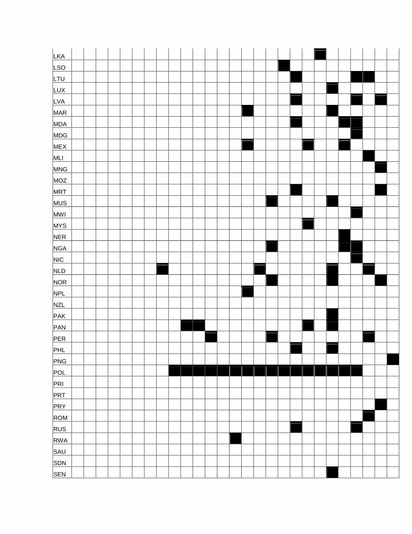
(This is graphically shown in Table 2 where a black box indicates that an observation is

available.) If we require, not unreasonably for a study that claims to have derived income

inequality statistics for each year over the period, that a country should have observations for

at least two-thirds of the time (that is, to have more than 18 observations), we are left with a

total of six countries: USA, Bulgaria, Taiwan, Great Britain, Canada and Japan. 21 Only one

country—the US—has observations for all the years.

Sala-i-Martin presents to the reader his results as if there we no blanks at all in the

data. As we already know, he gets round blank spots by extrapolating forward and backward

in time the results obtained from the years for which he has the data. Thus the Chilean black

18 Calculated by taking the 1996 GDP per capita (27,880 in 1995 international dollars) and multiplying by factors or 2.5 and 3.5. (If the top decile gets between 25 and 35 percent of total US income, then average per capita income of its members is between 2.5 and 3.5 times the US average.) 19 Calculated as follows. The US per capita GDP in 1996 was 3.72 times higher than the world GDP per capita. Then, the mean income of the top US decile is anything between 9.3 and 13 times mean world income. Since US top decile comprises about ½ of a percent of world population, their share in world income ranges between 4.7 and 6.5 percent. 20 The period covered by the Deininger-Squire database runs up to 1996. Sala-i-Martin’s data (thanks to WDIs) extend into 1998. The difference cannot but be minor. 21 And to complicate matters further, the Japanese surveys from which these data are derived are not nationally representative because they leave out farmers and one-person households, that is, ten percent of the population (see Tachibanaki and Yagi, 1997). And Bulgaria is, as we have seen, not included.

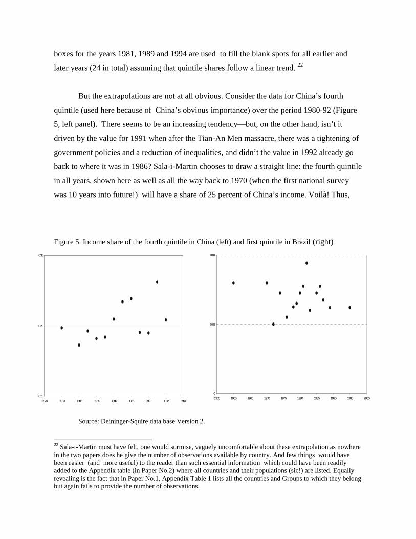
boxes for the years 1981, 1989 and 1994 are used to fill the blank spots for all earlier and

later years (24 in total) assuming that quintile shares follow a linear trend. 22

But the extrapolations are not at all obvious. Consider the data for China’s fourth

quintile (used here because of China’s obvious importance) over the period 1980-92 (Figure

5, left panel). There seems to be an increasing tendency—but, on the other hand, isn’t it

driven by the value for 1991 when after the Tian-An Men massacre, there was a tightening of

government policies and a reduction of inequalities, and didn’t the value in 1992 already go

back to where it was in 1986? Sala-i-Martin chooses to draw a straight line: the fourth quintile

in all years, shown here as well as all the way back to 1970 (when the first national survey

was 10 years into future!) will have a share of 25 percent of China’s income. Voilà! Thus,

Figure 5. Income share of the fourth quintile in China (left) and first quintile in Brazil (right)

Source: Deininger-Squire data base Version 2.

22 Sala-i-Martin must have felt, one would surmise, vaguely uncomfortable about these extrapolation as nowhere in the two papers does he give the number of observations available by country. And few things would have been easier (and more useful) to the reader than such essential information which could have been readily added to the Appendix table (in Paper No.2) where all countries and their populations (sic!) are listed. Equally revealing is the fact that in Paper No.1, Appendix Table 1 lists all the countries and Groups to which they belong but again fails to provide the number of observations.

0.15

0.25

0.35

1978 1980 1982 1984 1986 1988 1990 1992 1994

0

0.02

0.04

1955 1960 1965 1970 1975 1980 1985 1990 1995 2000

Table 2 get filled with black dots. For many countries quintile shares exhibit a large

variability: rather than moving in predictable ways, or being stable, they “jump” all around

(see Sala-i-Martin Appendix Figures, Paper No.2, or Brazil in Figure 3 here). One is

reminded of Samuelson’s quip: “yes, you can draw them as straight lines, but only with a very

thick chalk.”

So, after being treated to an estimate of the entire distributions from five data points,

we are now led for another leap into the unknown. These very dubious annual estimates are

now extrapolated to years vastly apart to get estimates of quintile shares throughout the entire

period. Here is the enormity of the assumptions. Data on income of the top 20% of (say)

Chileans in the year 1994 are used not only to infer the income of the top decile, or of the top

ventile in that year. They are also used to infer income of the bottom quintile and of the

bottom decile and of the bottom 15% or whatever (that is, of the entire distribution) in all

other years. 23 And thus for every country.

We have seen that for Group A and B countries (97 countries), observations are

available for, on average, only 5.5 out of 27 years. For 28 countries in Group C, there are no

data at all. This means that the overall time coverage is 15.8 percent—leaving aside the

former Soviet republics, Bulgaria, Yugoslavia, Vietnam, Iran etc. which are not included at

all.24 If in addition, we assume that for a distribution to be reasonably well described, we need

ten data points (ten deciles), the desirable number of data-points becomes 27 times 125 times

10 = 33750. Instead, Sala-i-Martin has 2667 data points,25 or 7.9 percent.

Here is the deep-rooted problem with Sala-i-Martin’s calculations. He tries to

overcome the problem of fragmentary data by imposing a distribution on them. Given the

very few data points—some of which may themselves be fitted approximations—it is a

dramatic oversimplification with an unknown bias. But in addition, he faces the problem of 23 This is because n-th quintile share in year t, influences our linear approximation of that and all other quintile shares (since the five shares have to add up to 1) in all the years for which one does the extrapolations. 24 Out of total maximum number of country/years, 27 times 125 = 3375, there are only 97 times 5.5 = 532 observations. 25 97 x 5.5 x 5.

data sparseness. He overcomes it by extending in time these largely arbitrary estimations

obtained from the country/years for which he had the data! “He then piled one simplifying

assumption upon another until, having really settled everything by these assumptions, he was

left with only a few aggregate variables between which, given these assumptions, he set up

simpler one-way relations so that, in the end, the desired results emerged almost as

tautologies.” Thus Schumpeter (1980 [1954], p. 472-3) defined the Ricardian vice.

In conclusion, to calculate true world inequality there is no shortcut from using the

individual-level data complemented (when individual data are unavailable) with grouped data

with at least decile shares. To do anything else, introduces a large and unknown degree of

arbitrariness in the results. This, combined with other problems (discussed below) and the

general issues that plague such calculations even if one had access to all individual-level data

(unequal reliability of surveys, differences in the definitions of welfare aggregates and the

like) makes the noise element dominate, by far, the signal.

4. Other problems We are not at the end of the problems yet. There are three more.

The first is the use of GDP per capita rather then survey means. This was done by

other authors as well (Chotikapanich, Valenzuela and Rao, 1997; Schultz 1998; Bhalla, 2002).

There are two problems with this approach. First, it introduces an inconsistency: we use and

trust household survey data for the distributions, but we do not believe their means. In other

words, surveys are good in guessing distributions, but they miss the means (income levels).

Some authors like Surjit Bhalla (2002) have insisted on this issue by claiming that survey

means (as is apparently the case in India) underestimate true income, and have erected the

negative difference between the survey means and GDP per capita from an issue that may (or

may not: the extensive debate on this in India is not conclusive) hold for India, into a general

proposition for all countries and all time. Second, the use of GDP per capita means that we

implicitly believe that over- or under-estimation of income by surveys is proportional to

reported income. If GDP per capita is 20 percent higher than the survey mean, by raising all

survey incomes by 20 percent we are claiming that under-reporting is proportional to reported

income. But, from the literature (see Ravallion, 2001 p. 1805; Ravallion, 2000, pp. 3250-1 in

the context of India, or Wagner and Grabka, 1999 for Germany) we know that this is not the

case. If there is a misstatement of survey incomes, it is most at low ends (where people are

missed by surveys) and top ends (where people hide their incomes, or where income types

associated with rich people are imperfectly reported). 26 As Ravallion (2000) writes, there is

an internal inconsistency in use of national accounts data instead of household survey means.

As the two have diverged in time in India, the adjustment factor by which survey means have

been raised, has also increased. But at the same time, the authors persist in increasing income

of all recipients by the same percentage for any given year. Thus, they need to argue that “the

rate underestimation is roughly constant between people at one date, but…it has risen over

26 There are several ways in which this underreporting takes place. First, there is “top-coding” (maximum acceptable value) for some income components like capital gains in the US Census Survey (top coded at $99,999 per household). Other countries (Germany) do the same. Second, there is a consistent underestimation of income sources associated with the rich. Property income is underestimated by 60 percent in France (Concialdi, 1997, p. 261) and by more than 40 percent in Germany (Wagner and Grabka, 1999).

time with growth in mean consumption (Ravallion, 2000, p. 3250). In conclusion, if we do not

believe survey levels, and want to correct them, adjusting them by the same percentage across

the board is very crude and almost surely wrong.

The second problem is mixing of income and expenditure data. This is the problem

present in Milanovic (2002) as well. It is made unavoidable by the fact that countries

“specialize” in having either income or expenditure surveys, and then the coverage of the

whole world by either income or expenditure surveys alone becomes impossible. Sala-i-

Martin, as well as the Deininger-Squire database, also mixes the two sources: the quintiles are

in some cases derived from expenditure (or consumption) shares, and in some from income

shares.

The third, and a very serious issue, is the mixing of quintile shares obtained from

distributions of households with quintile shares derived from distributions of individuals. One

is the distribution of households by household income, denoted D(H|Yh), and another is

distribution of persons by household per capita income, denoted D(p|Yp). 27 The latter is, of

course, the one that we want to use. Sala-i-Martin does not mention explicitly that he is

combining the two sources. However, by comparing the total number of observations used by

Sala-i-Martin from the Deininger-Squire data base (about 540) with the total number of both

household- and individual-based quintile shares available in the D-S base for the period after

1970 (about 600), and taking into account that about 50 observations (Bulgaria, Russia, Iran

etc.) have not been used, it becomes clear that Sala-i-Martin must have combined D(p|Yp) and

D(H|Yh) distributions. The D(H|Yh) distributions account for about 40 percent of the D-S

database. Thus, had they not been used, Sala-i-Martin’s number of observations would have

been significantly smaller (about 350). The use of the wrong distribution D(H|Yh) makes a

total mess of world inequality calculations as now the issues of family size (vastly different

between countries) and inconsistency in the recipient units entirely vitiate the calculations,

making them simply meaningless. The five data points representing a distribution of

households by total household income in a country X in a year t are now interpreted to be the

27 To complicate matters further, there are also distributions of households by household per capita income D(H|Yp) but they are few in numbers.

same as (i) the distribution of people by their per capita income, and is used to guess (ii) the

entire income distribution of people for year t, and (iii) for many years forward and backward. 28

Moreover, even here, and rather surprisingly, lurks an additional source of bias. For

some unknown reason, the Deininger-Squire data uses much more of household-based

D(H|Yh) information for the period up to the 1990’s. Table 3 gives the share of household-

vs. individual-based quintiles for each decade used by the Deininger-Squire. Since D(H|Yh)

distributions are generally more unequal than D(p|Yp) distributions, the overall (or average)

level of inequality in the 1990’s will tend to be relatively low. As a result, the actual increase

in inequality which took place in the decades of the 1980’s and 1990’s, and which is plain to

see when we control for the type of recipient—that is, if we include only observations based

on distributions of persons—will fail to show in the data when D(H|Yh) and D(p|Yp) are

mixed together. This is illustrated in Figure 6.

Table 3. The two types of distributions used in the Deininger-Squire database

Decade Observations based on D(p|Yp)

Observations based on D(H|Yh)

Share of D(H|Yh) observations in total

1960’s 32 43 0.57 1970’s 60 93 0.61 1980’s 123 105 0.46 1990’s 146 17 0.10

Source: Calculated from the Deininger-Squire database version 2.

28 Facing the same problem of mixing household- and person-based data (and also using the D-S database), Schultz (1999) decides not to do the mixing: “Without a theory or a reliable procedure for relating the processes generating household and person income distributions…I am reluctant to mix the data on households and persons, because ot could conceal important regularities” (p. 324).

Figure 6. Mean Ginis in each decade (1960’s to 1990’s)

Source: calculated from the Deininger-Squire database version 2

And it is not that the results in Figure 6 are driven by some odd high-Gini outliers in

the 1990’s. Figure 7 (left panel) shows the distribution of the Ginis in the 1970’s and 1990’s

when persons and households are mixed up: the two distributions are practically the same.

Figure 7 (right panel) shows the distribution of countries’ Ginis when the concept (income

per capita across persons) is held constant. Now, it is not only that the mean and the median

Gini are higher in the 1990’s—the entire distribution of the Ginis has shifted rightward. This

is hardly surprising since we know that in the 1990’s there was another bout of increases in

inequality, this time in transition countries, China, India and parts of Latin America. The use

of the mixed household- and individual- data will then additionally bias Sala-i-Martin’s

calculations downward. It is important to note, however, that this effect is accidental: it just so

happened that the D-S database includes less of household-based observations in the 1990’s.

Yet, the problem highlights the more general issue of careless combination of the data where,

30

32

34

36

38

40

1960's 1970's 1980's 1990's

Gin

is

Keeping the same concept (only persons)

Using both persons and households

driven by the need to stretch the number of observations way beyond what the data allow, one

commits biases whose very direction cannot be gauged.

Figure 7. Distribution of Gini coefficients from the Deininger-Squire data base

Mixing households and persons as recipient units Holding the recipient unit (person) constant

1990’s

1970’s

yy20 40 60 80

0

.02

.04

.06

yy20 40 60 80

0

.02

.04

.06

1970’s

1990’s

5. The bottom line

The bottom line is that it is not surprising the purported Concept 3 inequality as

calculated by Sala-i-Martin behaves almost identically as the Concept 2 inequality (see Figure

8) . This is because the “fitting” of distributions based on very fragmentary data, plus the

extrapolations in time, had emptied out almost all variability from the within-country

component. Basically, within-country inequality is fixed—by the elimination of

“troublesome” (high inequality) countries, by the minimization of distributions’ variability

through the use of very few data points and linear extrapolations, by the assumption that all

countries whose distributions are unavailable exhibit perfect equality, and by the mixing of

household- and person-based distributions. It is the within-country inequality, which

superimposed onto Concept 2 inequality, yields inequality among world’s individuals. If

within-country inequality is fixed (and countries’ relative positions do not change much),29

then what is superimposed on the Concept 2 inequality is simply a shift parameter.

It is not surprising then that the evolution through time of what is ostensibly a Concept

3 inequality will be the same as the evolution in time of the Concept 2 inequality—as indeed

we see in Figure 8. One might conclude that what Sala-i-Martin has ended up by producing

is inequality between population-weighted GDPs per capita which simply masquerades as

inequality between individuals, or more exactly, a Concept 2 inequality with a constant shift

parameter.

29 Note that even if all within-country distributions are unchanged, but some countries grow faster (or slower) than others (so that their relative position changes), inequality between individuals of the world will change too.

Figure 8. Sala-i-Martin Concept 3 inequality and inter-national population weighted

inequality

While Sala-i-Martin’s results move in parallel with the Concept 2 inequality, they

move out of step with all other calculations of Concept 3 inequality. Figure 9 confronts Sala-i-

Martin’s results with other authors who have tried to calculate world inequality among

individuals. Sala-i-Martin’s is the only calculation that shows inequality steadily decreasing

during the last 30 years. All others show inequality on the rise, or going up and down without

an apparent trend. Sala-i-Martin results give also, by far, the lowest Gini of all other

calculations. Around 1993, the median estimate of other calculations is Gini between 64-65.

Sala-i-Martin’s Gini is 61.

40

45

50

55

60

65

70

1970

1971

1972

1973

1974

1975

1976

1977

1978

1979

1980

1981

1982

1983

1984

1985

1986

1987

1988

1989

1990

1991

1992

1993

1994

1995

1996

1997

1998

Gin

i co

effi

cien

t

Sala-I-Martin calculation

Concept 2 inequality

Figure 9. Sala-i-Martin’s calculations confronted to others

Sources: Milanovic (2002 and for 1998 estimate from 2002a), Bourguignon and Morrisson (1999), Dikhonov and Ward (2001), Dowrick and Akmal (2001). To conclude, Sala-i-Martin has succumbed to the temptation of piling one

assumption upon another with the result that neither the author, nor the reader can any longer

tell which is the part of each assumptions, individually or together, in deriving the final result.

Here are, in summary, the Ricardian building blocks used by Sala-i-Martin in his

calculations—with (*) signs indicating the assumptions imparting unambiguous downward

bias to the results:

1. (*) A strange omission of countries with “disturbing rises” in inequality; then,

2. Use five data points to approximate entire distributions. 3. When these five data points are not available (84 percent of the time), extrapolate

backward and forward in time. When only one observation is available; assume

56

58

60

62

64

66

68

70

1970

1971

1972

1973

1974

1975

1976

1977

1978

1979

1980

1981

1982

1983

1984

1985

1986

1987

1988

1989

1990

1991

1992

1993

1994

1995

1996

1997

1998

1999

Dikhanov-Ward

Bourgignon-Morrison

Milanovic

Dowrick-Akmal

Sala-I-Martin

Chotiapanich-Val.-Rao

distribution stays the same for 30 years; (*) when there is no observation at all, assume everybody in the country has the same income.

4. (*) Treat distributions of household income across households as if they were

distributions of per capita income across individuals. 5. Mix National accounts data (GDP per capita) and household survey data. 6. Mix expenditure and income data.

and produce world income distribution across individuals of the world for the last

thirty years. To paraphrase, “never was so much calculated with so little.” And, unfortunately,

it shows.

REFERENCES:

Bourguignon, Francois and Christian Morrisson (1999). “The size distribution of income among world citizens, 1820-1990”, manuscript (June). Forthcoming in American Economic Review, September 2002.

Bhalla, Surjit (2002), Imagine there is no country, Washington: Institute for

International Economics. Chotikapanich, D., Valenzuela, R. and Rao, D.S.P. (1997). “Global and

regional inequality in the distribution of income: estimation with limited and incomplete data.” Empirical Economics, vol. 22, pp. 533-546.

Pierre Concialdi (1997), "Income Distribution in France: the mid-1980's turning

point" in Peter Gottschalk, Bjorn Gustafson, and Edward Palmer (eds.), Changing patterns in the distribution of economic welfare. An international perspective, Cambridge: Cambridge University Press.

Dikhanov, Yuri and Michael Ward (2001), “Evolution of the Global Distribution

of Income, 1970-99”, August 2001 draft. Dowrick, Steve and Muhammed Akmal (2001), “Contradictory Trends in

Global Income Inequality: A Tale of Two Biases”, draft 29 March 2001, available from http://ecocomm.anu.edu.au/economics/staff/dowrick/dowrick.html.

Maddison, Angus (1995), Monitoring the World Economy, 1820-1992,

Paris:OECD Development Centre Studies. Maddison, Angus (2001), The World Economy: A Millennial Perspective,

Paris:OECD Development Centre Studies. Melchior, Arne, Kjetil Telle and Henrik Wiig (2000), “Globalisation and

Inequality: World Income Distribution and Living Standards, 1960-1998”, Royal Norwegian Ministry of Foreign Affairs, Studies on Foreign Policy Issues, Report 6B:2000, October.

Milanovic, Branko (2002), “True world income distribution, 1988 and 1993: First calculation based on household surveys alone” Economic Journal, January 2002, pp. 51-92.

Milanovic, Branko (2002a), “Worlds apart: the twentieth century’s promise

that failed”, manuscript. Available at www.worldbank.research/inequality.

Mukand, Sharun and Dani Rodrik (2002). “In search of the holy grail: policy convergence, experimentation, and economic performance”, mimeo, January 2002. Available at http://ksghome.harvard.edu/~.drodrik.academic.ksg/papers.html.

Quah, Danny (1997), “Empirics for growth and distribution: stratification, polarization and convergence clubs”, London School of Economics and Political Science, Center for Economic Performance Discussion Paper No. 324, pp. 1-29.

Quah, Danny (1999), “6 x 109: Some Dynamics of Global Inequality and

Growth”, typescript, December 1999. Available at < http://econ.lse.ac.uk/staff/dquah/p/9912sbn.pdf>.

Quah, Danny (1999), “Calculations of world income distribution”, unpublished

notes.

Quah, Danny (2002), “One third of the world’s growth and inequality”, mimeo, March 2002. Ravallion, Martin (2000), “Should poverty measures be anchored to the National Accounts”, Economic and Political Weekly, August 26-September 2, 2000, pp. 3245-3252. Ravallion, Martin (2001), “Growth, inequality and poverty: Looking beyoind averages”, World Development, vol. 29, No. 11, pp. 1803-1815. Sala-i-Martin, Xavier (2002), “The Disturbing ‘Rise’ of World Income Inequality”, NBER Working paper No. 8904, April. Available at www.nber.org. Sala-i-Martin, Xavier (2002), “The World Distribution of Income”, NBER Working paper No. 8905, May. Available at www.nber.org.

Schultz, T. P. (1998). “Inequality in the distribution of personal income in the world: how it is changing and why.” Journal of Population Economics, vol. 11, No. 3, pp. 307-344.

Schumpeter, Joseph (1980[1954]), History of Economic Analysis, New York:

Oxford University Press. Tachibanaki, Toshiaki and Tadashi Yagi (1997), “Distribution of economic

well-being in Japan: towards a more unequal society” in Peter Gottschalk, Bjorn Gustafson, and Edward Palmer (eds.) Changing patterns in the distribution of economic welfare. An international perspective, Cambridge University Press, pp. 108-131.

Wagner, Gert and Markus Grabka (1999), “Robustness Assessment Report” [refers to German Socio-economic Panel 1994]. Available at http://www.lisproject.org/techdoc/ge/ge94survey.doc.

Table 1. List of countries and number of observations in Deininger-Squire data base (version 2), period 1970-96

United States of America 27 Panama 5 Turkey 2 Bulgaria 24 Surinam 5 Tanzania 2 Taiwan 23 Czech Rep 4 Uganda 2 United Kingdom 22 Dominican Rep 4 Uzbekistan 2 Canada 18 Estonia 4 Vietnam 2 Japan 18 Ghana 4 Burkina Faso 1 Poland 17 Iran 4 Bolivia 1 Italy 16 Peru 4 Barbados 1 Brazil 15 Philippines 4 Botswana 1 Sweden 15 Portugal 4 Central African Rep 1 Finland 13 Tunisia 4 Chile 1 India 13 Zimbabwe 4 Cameroon 1 Netherland 13 Belgium 4 Djibouti 1 China 12 Chile 4 Ecuador 1 New Zealand 12 Greece 3 Ethopia 1 Australia 11 Guatemala 3 Fiji 1 Bahamas 11 Ireland 3 Guinea 1 Indonesia 10 Jordan 3 Gambia 1 Venezuela 10 Lithuania 3 Guinea Bissau 1 Costa Rica 9 Latvia 3 Guyana 1 Yugoslavia 9 Moldova 3 Israel 1 Bangladesh 8 Mauritius 3 Kenya 1 Colombia 8 Nigeria 3 Laos 1 Czechoslovakia 8 Romania 3 Lesotho 1 Spain 8 Slovakia 3 Madagascar 1 Jamaica 8 Slovenia 3 Mali 1 Norway 8 Trinidad & Tobago 3 Mongolia 1 Pakistan 8 Ukraine 3 Malawi 1 Germany 7 Belarus 2 Niger 1 Hong Kong 7 Algeria 2 Nicaragua 1 Honduras 7 Egypt 2 Nepal 1 Hungary 7 Gabon 2 Papua New Guinea 1 Korea, South 7 Kazakhstan 2 Paraguay 1 Sri Lanka 7 Kyrgyz 2 Rwanda 1 Denmark 6 Luxembourg 2 Senegal 1 France 6 Morocco 2 Sierra leone 1 Malaysia 6 Mauritania 2 Yemen 1 Singapore 6 Puerto Rico 2 South Africa 1 Thailand 6 Russia 2 Switzerland 1 Cote d'Ivoire 5 El Salvador 2 Armenia 1 Mexico 5 Seychelles 2 Austria 1 Turkmenistan 2 Total 630

Table 2. Quintiles available in Deininger-Squire data base

(cases where recipients are persons) and used by Sala-i-Martin code 70 71 72 73 74 75 76 77 78 79 80 81 82 83 84 85 86 87 88 89 90 91 92 93 94 95 96

AGO

ALB

ARG

ARM

AUS

AUT

BEL

BEN

BFA

BGD

BGR

BHS

BLR

BOL

BRA

BRB

BWA

CAF

CAN

CHE

CHL

CHN

CIV

CMR

COG

COL

CRI

CSK

CZE

DEU

DJI

DNK

DOM

DZA

ECU

EGY

ESP

EST

ETH

FIN

FJI

FRA

GAB

GBR

GHA

GIN

GMB

GNB

GRC

GTM

GUY

HKG

HND

HRV

HTI

HUN

IDN

IND

IRL

IRN

ISR

ITA

JAM

JOR

JPN

KAZ

KEN

KGZ

KHM

KOR

KWT

LAO

LKA

LSO

LTU

LUX

LVA

MAR

MDA

MDG

MEX

MLI

MNG

MOZ

MRT

MUS

MWI

MYS

NER

NGA

NIC

NLD

NOR

NPL

NZL

PAK

PAN

PER

PHL

PNG

POL

PRI

PRT

PRY

ROM

RUS

RWA

SAU

SDN

SEN

SGP

SLE

SLV

SUN

SVK

SVN

SWE

SYC

TCD

TGO

THA

TKM

TTO

TUN

TUR

TWN

TZA

UGA

UKR

URY

USA

UZB

VEN

VNM

YEM

YUF

YUG

ZAF

ZAR

ZMB

ZWE