What determines income distribution and how income

distribution might affect growth

Branko MilanovicWorld Bank Training Poverty and Inequality Analysis

CourseMarch 3, 2011

A. From Kuznets to Piketty: determinants of income

distribution

1. Relationship between income and inequality: the rise and fall of

the Kuznets hypothesis

Kuznets inverted U-shaped curve (defined in 1955)

• As income increases, inequality at first goes up and then declines

• “It seems plausible to assume that in the process of growth, the earlier periods are characterized by…forces that may have widened the inequality…for a while because of the rapid growth of the non-A [non-agricultural] sector and wider inequality within it.

• It is even more plausible to argue that the recent narrowing in income inequality observed in the developed countries was due to a combination of • the narrowing inter-sectoral inequalities in product per worker, • the decline in the share of property incomes in total incomes of households, and • the institutional changes that reflect decisions concerning social security and full employment."

Kuznets curve: history• Evidence for Kuznets curve in cross-sectional

data analyzed in the 1970s, 1980s (Paukert, Lecaillon, Koeble & Thomas)

• More than 90% of pooled time-series and cross-sectional Gini variability is due to differences between countries => factors that determine country inequality are stable (Li, Squire, Zhou)

• Elusive evidence in time-series (Oshima)• Strong historical evidence for Western Europe

before and during Industrial revolution (Lindert and Willianson, van Zanden, Prados)

• Modifications of the Kuznets curve: “strong” and “weak” formulations

The same idea; Tocqueville 120 years earlier

• If one looks closely at what has happened to the world since the beginning of society, it is easy to see that equality is prevalent only at the historical poles of civilization. Savages are equal because they are equally weak and ignorant. Very civilized men can all become equal because they all have at their disposal similar means of attaining comfort and happiness. Between these two extremes is found inequality of condition, wealth, knowledge-the power of the few, the poverty, ignorance, and weakness of all the rest. (Memoir on pauperism, 1835).

• General formulation (used by Ahluwalia 1976)

• We expect β1>0 and β2<0

• Control variables include socialist dummy, government transfers, share of state sector employment, openness, age structure of population (Milanovic 1994; Williamson and Higgins 1999)

itt

k

ikititoit eZYYGini 221 )(lnln

Relationship between Gini and GDP per capita; (about 1100 Ginis between 1970 and 2005)

twoway (scatter Giniall lngdpppp if Giniall<65) (qfit Giniall lngdpppp, yline(20 60, lpattern(dash))), legend(off) xtitle(ln of GDP per capita in international dollars) ytitle(Gini)From global_new2.dta

Kuznets curve

20

30

40

50

60

Gin

i

6 7 8 9 10 11ln of GDP per capita in international dollars

• No controls; a weak inverted U relationship (more than 1300 Gini obs)

• Huge variability in inequality; R2 only 0.11• The upward sloping part of the curve

generally hard to discern• Turning point quite unstable; here about

$PPP 4,000 (level of Sri Lanka or Paraguay in 2008)

• Some disenchantment with the hypothesis: hard to see inverted U in time-series for a single country

No downward portion plotted against time or income: example of the USA

3035

4045

gini

WY+

gini

W in

that

ord

er o

f pre

cede

nce

1950 1960 1970 1980 1990 2000year when the survey was conducted

twoway scatter Giniall year if contcod=="USA", connect(l) ylabel(30(5)45)From allginis.dta.

3035

4045

Gin

i fro

m m

y al

lGin

i file

25000 30000 35000 40000 45000constant 2005 ppp, based on icp05

twoway scatter Giniall gdpppp if contcod=="USA", connect(l) ylabel(30(5)45)From global_new2

Example of China

3035

4045

Gin

i fro

m m

y al

lGin

i file

0 1000 2000 3000 4000constant 2005 ppp, based on icp05

Against income, 1970-2004

twoway scatter Giniall gdpppp if contcod=="CHN" & year<2005, connect(l) ylabel(30(5)45)From global_new2.dta

3035

4045

gini

WY+

gini

W in

that

ord

er o

f pre

cede

nce

1950 1960 1970 1980 1990 2000year when the survey was conducted

Against time, 1950-2004

twoway scatter Giniall year if contcod=="CHN" & year<2005, connect(l) ylabel(30(5)45)Based on giniall.dta

2. Credit market imperfections theory : “pull yourself by your

bootstraps”

Credit market imperfections• Poor households do not invest in human K even

if the returns are high; they invest in subsistence-related types of investment

• Indivisibilities: minimum threshold of K needed for investment; convex returns

• Societies with these problems both more unequal and wasteful in terms of human and capital resources

• Example of win-win strategy (inequality&growth)• Solutions: asset redistribution, no school fees,

deeper capital markets, micro finance

Credit constraint, education, democracy (Li, Squire & Zhou)

pooled IV formulation

Schooling 1960 -4.6** -4.4**

Democracy 1.6** 1.5**

Land Gini 60 0.16** 0.15**

Financial depth (M2/GDP)

-7.7** -10.1**

R2 0.62

No. of obs. 166 166

3. Political theory of income distribution

Methodologically, move from household survey data to fiscal

data

Long-run studies using income and inheritance tax data (Picketty et al.): France 1901-98

• Secular decline in inequality• Due to the declining share of top 1%• Due to the decreasing importance of large

capital income• Due to progressive taxation and

progressive (and high) inheritance taxes• Produces no effect on average K stock but

truncates large K holdings (lower concentration of capital income)

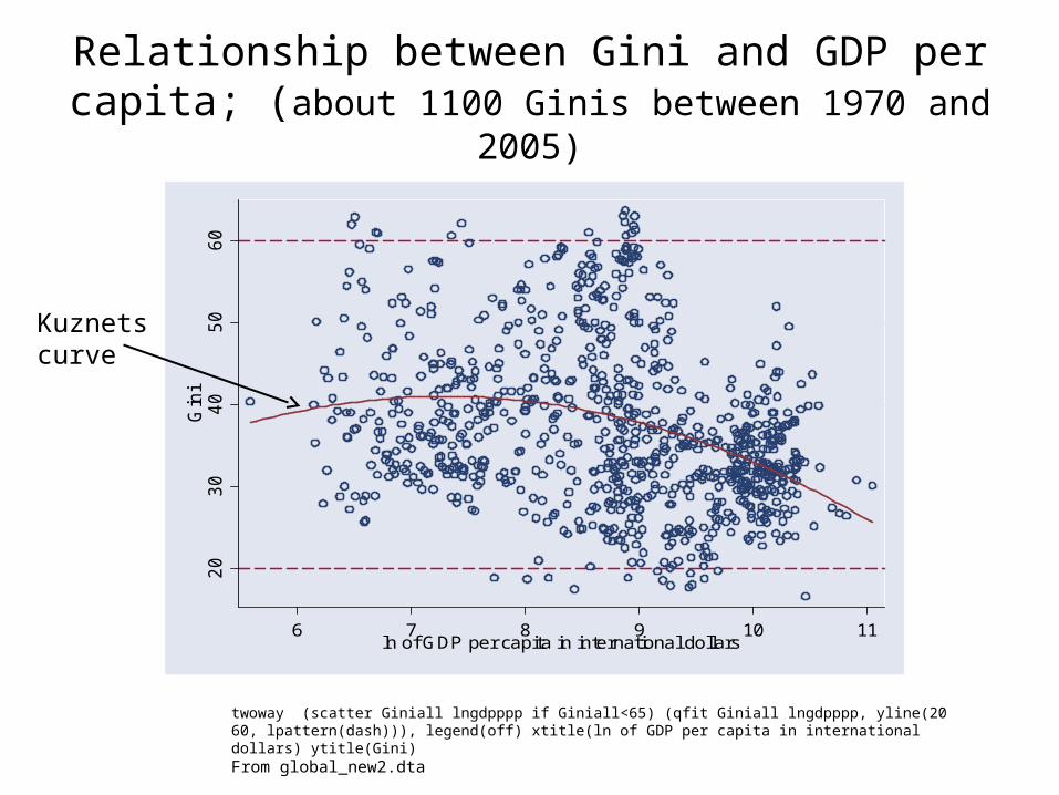
Story for the US (Piketty & Sanz)• Top K incomes decreased during the

Depression and WW2 and never recovered (top estates still lower in real terms than around 1900)

• Total K income did not decrease; its concentration did

• Change in factoral income composition among the top 1%; no longer mostly capitalists but salaried workers. Δ more pronounced in the US than in France

• Conclusion: No spontaneous decline in inequality. Role of depression, wars and progressive taxation. Policy and politics matter the most. A political theory of income distribution

Explanation by E. Saez in “Striking it richer”

The labor market has been creating much more inequality over the last thirty years, with the very top earners capturing a large fraction of macroeconomic productivity gains. A number of factors may help explain this increase in inequality, not only •underlying technological changes but also the retreat of institutions developed during the New Deal and World War II - such as • progressive tax policies, • powerful unions, • corporate provision of health and retirement benefits, and • changing social norms regarding pay inequality.

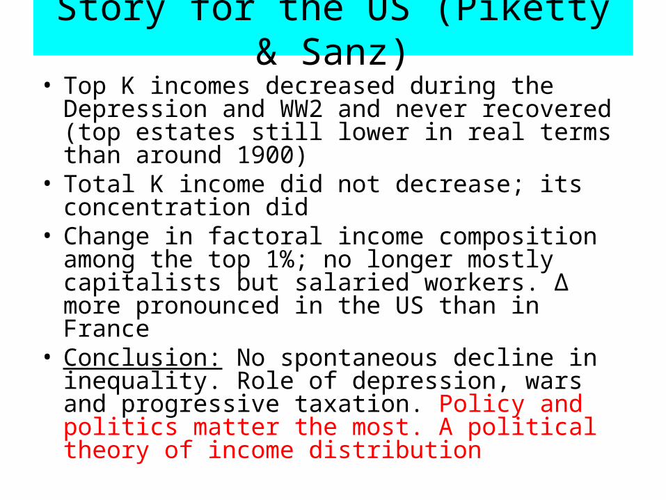
Recent findings

• A number of similar studies for developed countries reaches the same conclusion: a U-shaped inequality in the 20th century in English-speaking countries (UK: Atkinson 03; Netherlands: Atkinson & Salvedra 03; Italy: Brandolini)

• But also for India: Banerji and Piketty 2005• Long L shaped curve for the rest of

developed countries

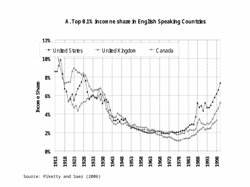
A. Top 0.1% incomne share in English Speaking Countries

0%

2%

4%

6%

8%

10%

12%

1913

1918

1923

1928

1933

1938

1943

1948

1953

1958

1963

1968

1973

1978

1983

1988

1993

1998

Inco

me

Sha

re

United States United Kingdom Canada

Source: Piketty and Saez (2006)

Fig 5. Top 0.1% income share in Germany and Japan

0%

2%

4%

6%

8%

10%

12%18

8518

9018

9519

0019

0519

1019

1519

2019

2519

3019

3519

4019

4519

5019

5519

6019

6519

7019

7519

8019

8519

9019

9520

00

Inco

me

Sha

re

Japan Germany

Source: Piketty and Saez (2006)

Fig 3: Share and Composition of top 0.01% in the US

0.0%

0.5%

1.0%

1.5%

2.0%

2.5%

3.0%

3.5%

4.0%

4.5%19

16

1921

1926

1931

1936

1941

1946

1951

1956

1961

1966

1971

1976

1981

1986

1991

1996

Salaries Business Income Capital Income Capital Gains

Source: Piketty and Saez (2006)

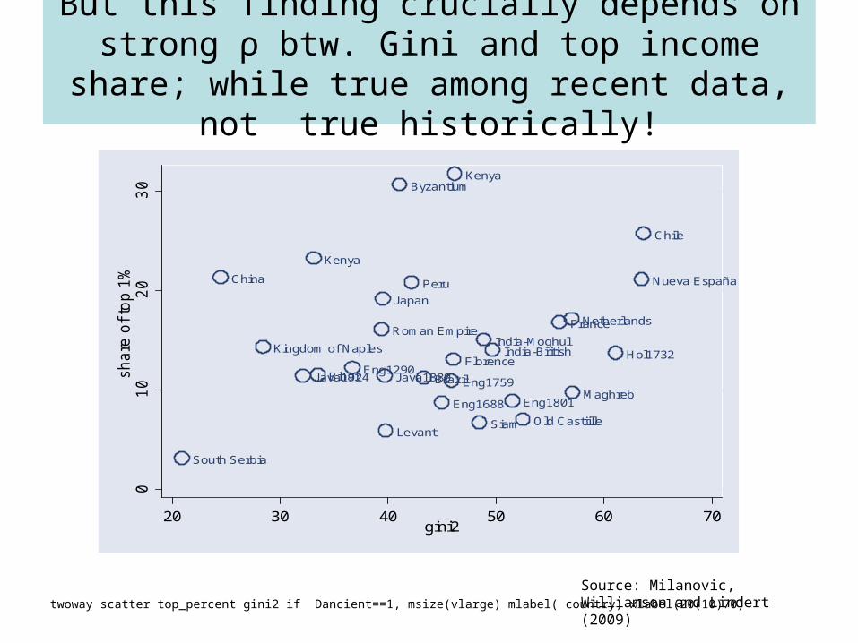
But this finding crucially depends on strong ρ btw. Gini and top income share; while true among

recent data, not true historically!

twoway scatter top_percent gini2 if Dancient==1, msize(vlarge) mlabel( country) xlabel(20(10)70)

Source: Milanovic, Williamson and Lindert (2009)

Roman Empire

Byzantium

Eng1290Florence

South Serbia

Levant

Eng1688

Hol1732India-Moghul

Old Castiille

Eng1759

France

Nueva España

Eng1801

Bihar

Netherlands

Kingdom of Naples

Chile

Brazil

Peru

Maghreb

China

Java1880

Japan

Kenya

Java1924

Kenya

Siam

India-British

01

02

03

0sh

are

of to

p 1

%

20 30 40 50 60 70gini2

B. How inequality might affect growth

Channel 1: The median voter hypothesis (Meltzer-Richard)

Political mechanism• Greater inequality in

factor income=>• Relatively poor μ

voter=>• Chooses relatively

high tax rate

Economic mechanism• High redistribution

and distorsionary effect of taxes =>

• Lower growth rate

Extent of redistribution = = fct (inequality in market income)

• Hypothesis 1. More market-unequal countries redistribute more (using two definitions of market income, without and with government pensions)

• Hypothesis 2. An increase in market share of a given decile is associated with a lower sharegain

• Question. If countries do redistribute more, is the mechanism through which it happens, the median voter hypothesis?

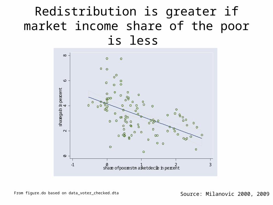
Redistribution is greater if market income share of the poor is less

Source: Milanovic 2000, 2009

02

46

8sh

areg

ain

in p

erce

nt

-1 0 1 2 3share of poorest market decile in percent

From figure.do based on data_voter_checked.dta

It holds for all deciles: if a decile is better-off in terms of marketP income distribution, it loses more through the redistribution

02

46

8sh

areg

ain

in p

erce

nt

-1 0 1 2 3share of poorest market decile in percent

01

23

45

shar

egai

n in

per

cent

1 2 3 4 5share of poorest market decile in percent

Bottom (first) decile Second decile

Richest (top) decile Second richest decile

-8-6

-4-2

0sh

areg

ain

in p

erce

nt

20 25 30 35share of poorest market decile in percent

-3-2

-10

shar

egai

n in

per

cent

15 16 17 18share of poorest market decile in percent

More market unequal states of the world associated with greater Gini reduction through redistribution

Without controls With controls

Gini of marketP income +0.438**(8.9)

+0.473**(8.2)

Openness +0.002(0.9)

GDP per capita (in logs) -0.004(-0.6)

Constant -0.010**(-5.3)

-0.070(0.3)

R2 (within) 0.47 0.54

Number of observations 110 100

Dependent variable: Gini reduction through redistribution. Country fixed effects regression. Source: Milanovic (2009)

But we cannot show that the middle deciles gains more if market inequality high

-8-6

-4-2

0ga

in o

f the

mid

dle

36 38 40 42 44 46share of the middle in market income

Source: Milanovic 2000

Sharegain of the very poor, 1973-2005 (using market income)

USA

Germany

24

68

10

Dis

trib

utio

na

l ga

in o

f th

e b

ottom

de

cile

1970 1980 1990 2000 2010year

twoway (scatter gain3 year if contcod=="DEU" & decile==1, connect(l)) (scatter gain3 year if contcod=="USA" & decile==1, connect(l)), legend(off) text(4 2000 "USA") text(7 2000 "Germany") ytitle(Distributional gain of the bottom decile) Based on data_voter_checked.dta

Channel 2: Inequality and property rights

Political mechanism• Greater inequality

creates cleavages =>• They are particularly

strong if coincide with ethnic differences (high horizontal inequality)=>

• Insecure property rights

Economic mechanism• Insecure property

rights =>• Lower growth rate

Inequality and property rights (Keefer & Knack)

Dependent variable:

protection of property rightsCross section

Ln GDP per capita 1985 7.61**

Ethnic tensions -0.933**

Income Gini circa 1985 -0.196**

Land Gini 1985 -0.097**

R2 0.80

No. of obs. 64

Dependent variable: Property rights: ICRG measure 1986-95. Ranges from 0 to 50.

Excursus: the reverse link and the reverse sign: greater protection of property rights

increases inequalityDependent Gini Gini (time-dummies

included on the RHS)

Property rights 0.929** 0.709*

Financial development (M2/GDI)

-0.064** -0.07**

Education 0.026 -0.016

Land inequality -0.016 -0.02

Democracy 0.438** 0.323**

Prop. Rights x Democracy

-0.056** -0.046**

R2 within (N) 0.26 (203) 0.35 (203)

• Greater protection of property rights increases inequality

• The rich elite is also politically powerful and protects its economic assets

• The effect is mitigated by the introduction of democracy

• => The negative effect of property rights protection is particularly strong in low-democracy environments

• But the regression does not include an income term

(results based on Savoia and Easaw, 2007; World Development, Feb. 2010)

Channel 3. Inequality caused by “morally irrelevant” characteristics

• Inequalities which are independent of individual effort, entrepreneurship or luck

• “Wasteful” (vs. instrumental or “useful”) inequalities

• Examples: education, health, opportunity to better oneself economically, to have a political voice

• Horizontal inequalities between ethnic/religious groups, education levels, socio-economic categories, geographical areas

Assumed ρ’s for different parts of the world

Base case Optrimistic (high mobility)

Pessimistic (low

mobility)

Average Gini (year 2002)

Nordic 0.2 0.15 0.3 27.5

Rest WENAO

0.4 0.3 0.5 33.7

E. Europe 0.4 0.3 0.5 30.6

Asia 0.5 0.4 0.6 37.6

LAC 0.66 0.5 0.9 53.8

Africa 0.66 0.5 0.9 42.6

Also a super-optimistic: ρ=0.2 for all; and super-pessimistic: ρ=0.9 for all. ρ’s based on literature review.

How one’s income depends on circumstances:(dependent variable: own household per capita income, in $PPP, logs)

Eq.

Mean per capita country income (in ln)

Gini index (in %)

Parents’ estimated income class (ventile)

Constant

Number of observations

R2 adjusted

Number of countries

6 (Pessimistic)

0.991

(0)

-0.019

(0.00)

0.109

(0.00)

-0.582

(0.00)

232,000

0.83

116

4 (Base)

0.986

(0.00)

-0.019

(0.00)

0.105

(0.00)

-0.513

(0.00)

232,000

0.81

116

5 (Optimistic)

0.987

(0)

-0.019

(0.00)

0.100

(0.00)

-0.462

(0.00)

232,000

0.80

116

• Circumstances at one’s birth (country + parents’ income class) explain between 83 percent (if world is fairly income-mobile within countries) and 85 percent (if there is less social mobility) of variability in income globally

• => thus, only a very small portion of global income differences can be due to effort

• Coefficient on country mean income remains 1; coefficient on parental income 0.1 (each notch is worth 10% increase in children’s income); coeff. slightly higher if there is less social mobility

• As a proxy, WDR06 looks at the contribution of horizontal inequalities to total inequality, or total “feasible between- inequality” (total Y of country=given; number and sizes of groups=given; ‘pecking order’ by group mean incomes= given; => find new group mean incomes that maximize the between component)

• Up to 40-45% of “feasible between inequality” explained by education differences

• Inequality traps and the interaction between political and economic power