Brief User’s Guide: Dynamic Systems Estimation

(DSE)

Paul Gilbert

September, 2009. Copyright 1993-2009, Bank of Canada.

The user of this software has the right to use, reproduce and distribute it.The Bank of Canada makes no warranties with respect to the software or itsfitness for any particular purpose. The software is distributed by the Bank ofCanada solely on an ”as is” basis. By using the software, the user agrees toaccept the entire risk of using this software.

The software documented here is available on the the Comprehensive RArchive Network (CRAN) <http://cran.r-project.org>. Please check for newversions.

This Guide is generated automatically using the R Sweave utilities (see F.Leisch, R News v2/3, Dec. 2002, p 28-31), so the examples should all work.The text and examples are included in the distributed package subdirectoryinst/doc/dse-guide.Stex. Please check that file if there is any doubt about theexample code. The output from some of the examples is shown but, to conservepaper, much of the output is not shown. It is intended that users should workthrough the examples and see the output themselves.

I regularly use the code with R on Linux and sometimes on Windows. Thereis an extensive set of tests which is run on all R test platforms for packagesdistributed on CRAN. Please report any errors you find. In the past, the codehas also worked with Splus 3.3 on Solaris, but I no longer run this. There areknown problems with Splus since version 5.

Caveat: This software is the by-product of ongoing research. It is not acommercial product. Limited effort is put into maintaining the documentation(but the R tools do automatically check that all functions and their argumentsare documented in the help system, and all examples work). This guide mayhave references to functions which do not yet work and/or have not been dis-tributed, and the documentation may not correspond to the current capabilitiesof the functions (but please report these problems if you find them). While thesoftware does many standard time-series things, it is really intended for doingsome non-standard things. The main difference between dse and most widelyavailable software is that dse is designed for working with multivariate timeseries and for studying estimation techniques and forecasting models.

Constructive suggestions and comments are welcomed by the package main-tainer.

1

1 Introduction to dse

2 Getting Started

3 General Outline of dse Objects and Methods

4 Defining a TSdata Structure

5 ARMA and State-Space TSmodels

6 VAR and VARX TSmodels

7 Model Estimation

8 Forecasting, Etc

9 Evaluation of Forecasting Models

10 Adding New TSmodel Classes

11 Adding New TSdata Classes

12 Mini-Reference

Related Packages (not in this guide)

setRNG, tframe, EvalEst, CDNmoney, tsfa, TSdbi

2

1 Introduction to dse

dse was originally designed with linear, time-invariant auto-regressive moving-average (ARMA) models and state-space (SS) models in mind. These remainthe most well developed models and provide the basis for the examples in thisguide.

In order to provide examples, implemented estimation techniques and meth-ods for converting among various representations of time series models are usedin this guide. (However, it is possible to use dse structure and add other estima-tion techniques.) Many functions for the usual diagnostics which are preformedwith time series data and models are included in the package. Additional in-formation on specific functions is available through the help facility. For detailsof some of the underlying theory of ARMA and SS model equivalence and ex-amples of some of the capabilities of the dse packages see Gilbert (1993) 1. Forexamples where dse is used to evaluate estimation methods see Gilbert (1995) 2.Examples of the use of several functions are illustrated in the files in the demosubdirectories. (In R see demo(package=”dse”) )

2 Getting Started

These packages works with recent versions of the R language (Ihaka and Gen-tleman, 1996) 3 available at <http://cran.r-project.org>. Italics will be used toindicate functions and objects, and () is frequently added to function names tohelp distinguish them as such. Anything entered after a # is a comment in R.Most examples in this guide show only the user input, not the computer output.

If dse is not installed on your system, please use the usual R package instal-lation procedures. Once R is started the dse packages must be made available.

> library("dse")

The code from the vignette that generates this guide can be loaded into aneditor with edit(vignette(”Guide”, package=”dse”)). This uses the default editor,which can be changed using options().

Several data sets are included with dse and will be used in examples in thisguide. The names of the data sets can be listed with

> data(package="dse")

They are made available by

1P.D. Gilbert, 1993. ”State Space and ARMA Models: An Overviewof the Equivalence”, Bank of Canada working paper 93–4. Available athttp://www.bankofcanada.ca/1993/03/publications/research/working-paper-199/

2P.D. Gilbert, 1995. ”Combining VAR Estimation and State Space Model Reduction forSimple Good Predictions”, J. of Forecasting: Special Issue on VAR Modelling, 14, 229–250.

3R. Ihaka and R. Gentleman, 1996. ”R: A Language for Data Analysis and Graphics”,Journal of Computational and Graphical Statistics, 5(3), 299–314.

3

> data(eg1.DSE.data, package="dse")

> data(egJofF.1dec93.data, package="dse")

The dse package requires tframe. It and other required packages will beloaded automatically. Some functions (in particular, tfplot) are part of thetframe package.

Descriptions of functions and objects are available in the R help system oncethe packages are installed.

3 General Outline of dse Objects and Methods

dse implements three main classes of objects: TSdata, TSmodel, and TSes-tModel. These are respectively, representations of data, models, and modelswith data and estimation information.

TSdata is an object which contains a (multivariate) time series object calledoutput and optionally another called input. Methods for defining the generalversion of this class of object are described in the next section and more detailsare provided in the help for TSdata. Input and output correspond to what areoften labelled x and y in econometrics and time series discussions of ARMA mod-els. These are sometimes called exogenous and endogenous variables, thoughthose terms are often not correct for these models. Statistically, output is thevariable which is modelled and input is the conditioning data. From a practicaland computational point of view, the model forecasts output data and inputdata must always be supplied. In particular, to forecasts multiple periods intothe future requires supplying input data for the future so that the model cancalculate outputs. The terms input and output are commonly used in the en-gineering literature, and often correspond to a control variable and the outputfrom a physical system. However, the causal interpretation in this context is notalways appropriate for other uses of time series models. In addition, even whena causal direction is known or assumed, it is not always desirable to define theexogenous variable as an input. If the model is to give forecasts into the futurethen it may be better to define exogenous variables as outputs and let the modelforecast them, unless better forecasts of the exogenous variables are availablefrom other sources. One context in which an input variable is important is toexamine policy scenarios. In this context the policy variable is defined as theinput and forecasts are produced conditioned on different assumptions aboutthe policy.

TSmodel objects are models which are arranged to use TSdata. These objectsalways have another specific class indicating the type of model. The ARMA andSS constructor methods for ARMA TSmodels and state-space TSmodels aredescribed in a section below. Other specific classes of TSmodels can be definedand many of the methods in dse will work with these new models, as long asthey use TSdata and have a few important methods implemented. More detailson defining other classes of models are given in another section of this guide.Details on the representation of models are provided in the help for TSmodeland the help for specific model constructors.

4

TSestModel objects are objects which contain TSdata, a TSmodel, and somestatistical information generated by l(model, data). The l() method originallymeant likelihood, but the method returns the one-step-ahead predictions andother information based on those predictions. Methods for studying one-step-ahead model forecasts extract the predictions from these objects. Other methodstreat TSestModel objects as a simple way to group together a model and data.For example, methods for studying multi-step forecasts need to generate theforecasts, so they do not use the predictions in the TSestModel object. Moredetail about TSestModel objects is available in the help system.

The default method for TSdata() constructs a TSdata object, as will bedescribed in the next section. The generic methods TSmodel() and TSdata()can also be used to extract the TSmodel or TSdata object from another object(such as a TSestModel).

The functions in dse can be used by starting with data and estimating amodel, or by starting with a model and producing simulated data. The nextsection on TSdata starts with data, but it would be equally possible to startwith models as described in the sections on ARMA and State-Space TSmodels.

4 Defining a TSdata Structure

This section describes how to construct a TSdata structure if you have otherdata you would like to use. Some installations may have an online databaseand it may be possible to connect directly to this data. See the TSdbi packageregarding some possibilities for doing this.

For many people the situation will be that the data is in some ASCII file.This can be loaded into session variables with a number of standard R functions,the most useful of which are probably scan() and read.table(). Following is anexample which reads data from an ASCII file called ”eg1.dat” and puts it inthe variable called eg1.DSE.data (which is also one of the available data sets).The file is in the dse package directory otherdata. The file has five columnsof numbers and 364 rows. The first column just enumerates the rows and isdiscarded.

> fileName <- system.file("otherdata", "eg1.dat", package="dse")

> eg1.DSE.data <- t(matrix(scan(fileName),5, 364))[, 2:5]

This matrix can be used to form a TSdata object by

> eg1.DSE.data <- TSdata(input= eg1.DSE.data[,1,drop = F],

output= eg1.DSE.data[, 2:4, drop = F])

The matrix and the resulting TSdata object do not have a good time scaleassociated with points. A better time scale can be added by

> eg1.DSE.data <-tframed(eg1.DSE.data,

list(start=c(1961,3), frequency=12))

5

There are several different possibilities for representing time in R objects.The most common is the ts object, which is applied in the above default tframedmethod to both input and output. Either tframed or ts can also be used directlyon the matrix before the TSdata object is formed. The methods from the tframepackage are used extensively in the dse package because they extend to othertime representations in addition to ts, and provide a mechanism for extendingmethods to other objects like TSdata and TSmodels.

Names can be given to the series with

> seriesNamesInput(eg1.DSE.data) <- "R90"

> seriesNamesOutput(eg1.DSE.data) <- c("M1","GDPl2", "CPI")

Setting the series names is not necessary but many functions can use thenames if they are available. (This overlaps somewhat with dimnames, but is thepreferred method in dse as it extends to data which is not a matrix.) The TSdataobject with elements input and output is the structure which the functions indse expect. More details on this structure are available in the help for TSdata.The input and output elements can be defined in a number of different waysand new representations can be fairly easily added.

Once data is available a model can be estimated:

> model1 <- estVARXls(eg1.DSE.data)

> model2 <- estSSMittnik(eg1.DSE.data, n=4)

> # or model2 <- estSSMittnik(eg1.DSE.data) prompts for state dimension

(Note: these models are not the same as those reported in Gilbert,1993. Inthat paper a variant of estVARXar was used.) The scales of the different seriesin eg1.DSE.data are very different, with the result that the covariance matrixof the residuals from the estimation is nearly singular. This is detected duringthe calculation of residual statistics. Statistics are then calculated using onlythe non-degenerate subspace and a warning message is printed. A better modelmight be obtained if the data were scaled differently.

Information about the estimated models can be displayed, for example:

> summary(model1)

> summary(model2)

> model1

> model2

> stability(model1)

> stability(model2)

> informationTests(model1, model2)

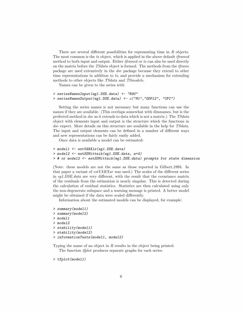
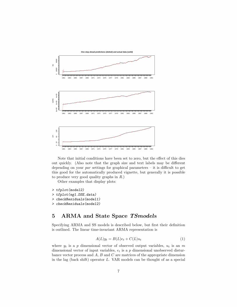
Typing the name of an object in R results in the object being printed.The function tfplot produces separate graphs for each series.

> tfplot(model1)

6

M1

1961 1963 1965 1967 1969 1971 1973 1975 1977 1979 1981 1983 1985 1987 1989 1991

010

000

3000

0

One step ahead predictions (dotted) and actual data (solid)G

DP

l2

1961 1963 1965 1967 1969 1971 1973 1975 1977 1979 1981 1983 1985 1987 1989 1991

0e+

002e

+05

4e+

05

CP

I

1961 1963 1965 1967 1969 1971 1973 1975 1977 1979 1981 1983 1985 1987 1989 1991

020

6010

0

Note that initial conditions have been set to zero, but the effect of this diesout quickly. (Also note that the graph size and text labels may be differentdepending on your par settings for graphical parameters – it is difficult to getthis good for the automatically produced vignette, but generally it is possibleto produce very good quality graphs in R.)

Other examples that display plots:

> tfplot(model2)

> tfplot(eg1.DSE.data)

> checkResiduals(model1)

> checkResiduals(model2)

5 ARMA and State Space TSmodels

Specifying ARMA and SS models is described below, but first their definitionis outlined. The linear time-invariant ARMA representation is

A(L)yt = B(L)et + C(L)ut (1)

where yt is a p dimensional vector of observed output variables, ut is an mdimensional vector of input variables, et is a p dimensional unobserved distur-bance vector process and A, B and C are matrices of the appropriate dimensionin the lag (back shift) operator L. VAR models can be thought of as a special

7

case of ARMA models with B(L) = I. ARIMA models are also a special caseof ARMA models.

A linear time-invariant state space representation in innovations form is givenby

zt = Fzt−1 + Gut + Ket−1

yt = Hzt + et

where zt is the unobserved underlying n dimensional state vector, F is thestate transition matrix, G, the input matrix, H, the output matrix, and K, theKalman gain. The first equation is commonly referred to as the state transitionequation and the second as the measurement equation.

dse also has some limited capabilities to work with the more general non-innovations form

zt = Fzt−1 + Gut + Qnt

yt = Hzt + Ret

where nt is the system noise, Q, the system noise matrix, and R the output(measurement) noise matrix.

Note that the time convention implies that the input variable ut can influ-ence the state zt and then the output variable yt in the same time period. Thisconvention is not always used in time-series models. It is important with eco-nomic data, especially at annual frequencies, that the input can influence theoutput in the same period. Another convention that is often used is to havethe output in the measurement equation depend on the state in the previoustime period. Then, to achieve the same objective, it is necessary to include theinput ut in the measurement equation as well. A different convention will alsoresult in slightly different algrebra converting between ARMA and state-spacemodels.

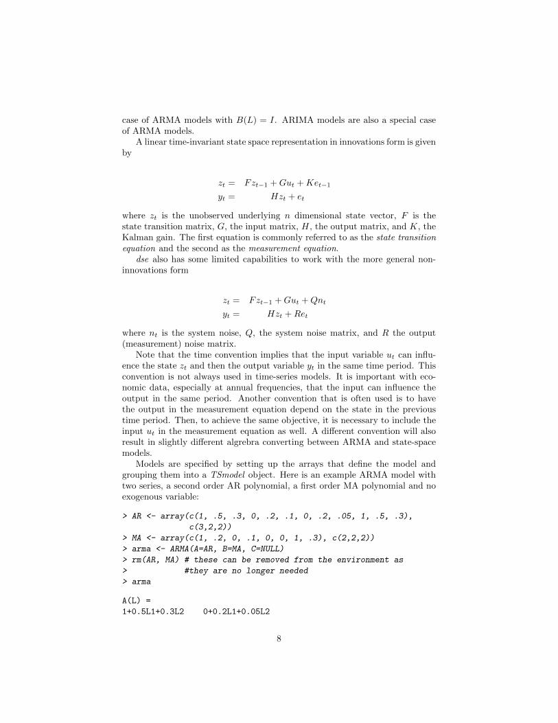
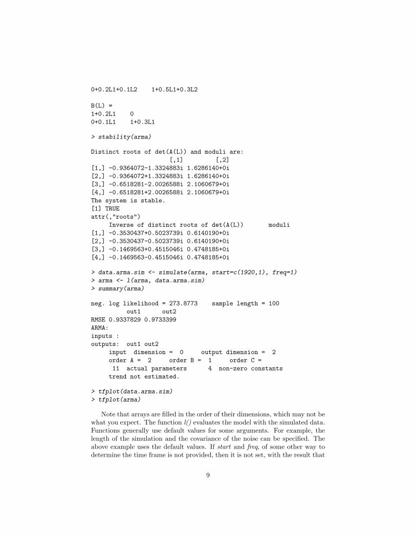
Models are specified by setting up the arrays that define the model andgrouping them into a TSmodel object. Here is an example ARMA model withtwo series, a second order AR polynomial, a first order MA polynomial and noexogenous variable:

> AR <- array(c(1, .5, .3, 0, .2, .1, 0, .2, .05, 1, .5, .3),

c(3,2,2))

> MA <- array(c(1, .2, 0, .1, 0, 0, 1, .3), c(2,2,2))

> arma <- ARMA(A=AR, B=MA, C=NULL)

> rm(AR, MA) # these can be removed from the environment as

> #they are no longer needed

> arma

A(L) =

1+0.5L1+0.3L2 0+0.2L1+0.05L2

8

0+0.2L1+0.1L2 1+0.5L1+0.3L2

B(L) =

1+0.2L1 0

0+0.1L1 1+0.3L1

> stability(arma)

Distinct roots of det(A(L)) and moduli are:

[,1] [,2]

[1,] -0.9364072-1.3324883i 1.6286140+0i

[2,] -0.9364072+1.3324883i 1.6286140+0i

[3,] -0.6518281-2.0026588i 2.1060679+0i

[4,] -0.6518281+2.0026588i 2.1060679+0i

The system is stable.

[1] TRUE

attr(,"roots")

Inverse of distinct roots of det(A(L)) moduli

[1,] -0.3530437+0.5023739i 0.6140190+0i

[2,] -0.3530437-0.5023739i 0.6140190+0i

[3,] -0.1469563+0.4515046i 0.4748185+0i

[4,] -0.1469563-0.4515046i 0.4748185+0i

> data.arma.sim <- simulate(arma, start=c(1920,1), freq=1)

> arma <- l(arma, data.arma.sim)

> summary(arma)

neg. log likelihood = 273.8773 sample length = 100

out1 out2

RMSE 0.9337829 0.9733399

ARMA:

inputs :

outputs: out1 out2

input dimension = 0 output dimension = 2

order A = 2 order B = 1 order C =

11 actual parameters 4 non-zero constants

trend not estimated.

> tfplot(data.arma.sim)

> tfplot(arma)

Note that arrays are filled in the order of their dimensions, which may not bewhat you expect. The function l() evaluates the model with the simulated data.Functions generally use default values for some arguments. For example, thelength of the simulation and the covariance of the noise can be specified. Theabove example uses the default values. If start and freq, of some other way todetermine the time frame is not provided, then it is not set, with the result that

9

plots may be for a matrix rather than a time series, that is, points instead of linegraphs. See the help on simulate for more details. In the example above, arma isinitially assigned an object of class TSmodel, but it is then re-assigned the valuereturned by l(), which is an object of class TSestModel. Also, many functionswork with different classes of objects, and do different things depending on theclass of the argument. The function tfplot() works with objects of class TSdataand TSestModel and also with time series matrices.

Here is an example of a state space model:

> f <- array(c(.5, .3, .2, .4), c(2,2)) #Note: do not use capital

> #F (=FALSE) as a variable name

> h <- array(c(1, 0, 0, 1), c(2,2))

> k <- array(c(.5, .3, .2, .4), c(2,2))

> ss <- SS(F=f, H=h, K=k) #F is argument name not variable name

> print(ss)

> stability(ss)

> data.ss.sim <- simulate(ss, start=c(1920,1), freq=1)

> ss <- l(ss, data.ss.sim)

> summary(ss)

> tfplot(ss)

Data which has been generated with simulate is a TSdata object and can beused with estimation routines. This provides a convenient way to generate datafor estimation algorithms, but remember that estimation will not necessarily getback to the model you start with, since there are equivalent representations (seeGilbert, 1993). However, a good estimate will get close to the likelihood andpredictions of the original model.

Here is an example of changing between state space and ARMA representa-tions using the models defined in the previous example:

> ss.from.arma <- l(toSS(arma), data.arma.sim)

> arma.from.ss <- l(toARMA(ss), data.ss.sim)

> summary(ss.from.arma)

> summary(arma)

> summary(arma.from.ss)

> summary(ss)

> stability(arma)

> stability(ss.from.arma)

The function roots() is used by stability() and can be used by itself to re-turn the roots but not evaluate their magnitude 4. When their arguments areTSmodels the functions toSS() and toARMA() return objects of class TSmodel

4By default the roots of an ARMA model are calculated by converting the model to statespace form, for reasons explained in Gilbert (2000, ”A note on the computation of time seriesmodel roots”, Applied Economics Letters, 7, 423–424). By specifying by.poly=T the methodcan be changed to use an expansion of the polynomial determinant.

10

which are not assigned to a variable in the above example, but used in the eval-uation of l(). The models are returned as part of the TSestModel returned byl().

For state space models there is often interest in the underlying state series.These can be extracted from an estimated model with the function state.

> tfplot(state(ss))

For an innovations form model the state is defined as an expectation givenpast information, so the Kalman filter estimates the state exactly. For an non-innovations form model the filter and smoother give slightly different estimates.(These are often called one-sided and two-sided filters in the economics liter-ature.) An innovations form model would usually be specified based on someadditional information about the structure of the system, typically a physicalunderstanding of the system in engineering, or some theory in economics. Inthe absence of this, an arbitary technique is to use a Cholesky decompositionto convert an innovations form model to an non-innovations form model.

The filter values are automatically returned by l() but, because of the addi-tional time and space requirements, the smoother values are not. The smootheris run separately by the function smoother().

> ssc <- toSSChol(ss)

> ssc <- smoother(ssc)

> tfplot(state(ssc, filter=TRUE))

> tfplot(state(ssc, smoother=TRUE))

These can be compared more easily with

> tfplot(state(ssc, smoother=TRUE), state(ssc, filter=TRUE))

The term state estimate is well established, but these should not be confusedwith model parameter estimates. The error in the model parameter estimatesconverges to zero as the length of the series increases to infinity (with goodestimators and assuming estimation assumptions are satisfied). State estimationerrors never converge to zero, and some authors prefer the term state predictionbecause of this. The state tracking error can also be extracted from an non-innovations form model.

6 VAR and VARX TSmodels

Vector auto-regressive models (VAR) and vector auto-regressive models withexogenous inputs (VARX) models are special cases of ARMA models covered inthe last section. (If you did not notice, please go back and re-read the previoussection.) For the moment, this section is only here because of the number oftime I get asked if dse can do VARs. Sometime I might add more special caseexamples here.

11

7 Model Estimation

The example data eg1.DSE.data and egJofF.1dec93.data are available with dseand are used in examples in this section.

To estimate an AR model with the default number of lags:

> model.eg1.ls <- estVARXls(trimNA(eg1.DSE.data))

In this example trimNA removes NA padding from the ends of the data,since the estimation method cannot handle missing values. This padding maynot be present, depending on how the data was retrieved. This data is highlycorrelated and highly parameterized models result in a degenerate covariancematrix. When this happens a warning is produced in this and other examples.

It is also possible to select a subsample of the data:

> subsample.data <- tfwindow(eg1.DSE.data, start=c(1972,1),

end=c(1992,12), warn=FALSE)

This creates a new variable with data starting in January 1972 and end-ing in December 1992. The R function window also usually works, howeverthe function tfwindow is typically used in dse and this guide because of someprogramming advantages. The argument warn=FALSE prevents some warningmessages from being printed. For example, when the specified start or end datecorresponds to the start or end date of the data, then the default warn=TRUEresults in a warning that the sample has not been truncated.

Various functions can be applied to the estimation result

> summary(model.eg1.ls)

> print(model.eg1.ls)

> tfplot(model.eg1.ls)

> checkResiduals(model.eg1.ls)

Other estimation techniques are available

> model.eg1.ar <- estVARXar(trimNA(eg1.DSE.data))

> model.eg1.ss <- estSSfromVARX(trimNA(eg1.DSE.data))

> model.eg1.bft <- bft(trimNA(eg1.DSE.data))

> model.eg1.mle <- estMaxLik(estVARXls(trimNA(eg1.DSE.data),

max.lag=1)) # see note below

tfplot can put multiple similar objects on a plot.

> tfplot(model.eg1.ls, model.eg1.ar)

> tfplot(model.eg1.ls, model.eg1.ar, start=c(1990,1))

Most of the estimation techniques have several optional parameters whichcontrol the estimation. Consult the help for the individual functions. estMax-Lik extracts data from a TSestModel and uses the model structure and initial

12

parameter values for the estimation. (Note: Maximum likelihood estimationcan be very slow and may not converge in the default number of iterations. Italso tends to over fit unless used with care, so that out-of-sample performanceis not good. I do not generally recommend it, although it does offer possibilitiesfor constraining the structure in specific ways (e.g. fixing some model matrixentries to zero or one). You might consider comparing mle to other estimationtechniques using functions discussed in the following sections and in the packageEvalEst.) In the above estMaxLik example a smaller (one lag) model is used.Be prepared for the estimation to take some time when models have a largenumber of parameters.

An important point to note is that the one-step-ahead predictions and relatedstatistics returned by these estimation techniques are calculated by evaluatingl(model, data) as the final step after the model has been estimated. This cangive different results than might be expected using the estimation residuals,particularly with respect to initial condition effects. (For stable models initialcondition effects should not be too important. If they are an important factorcheck the documentation for specific models regarding the specification of initialconditions.)

Also remember when estimating a model that, if you want to predict futurevalues of a variable, it will need to be an output in the TSdata object.

For the next example a four variable subset of the data in egJofF.1dec93.datawill be used. This subset is extracted by

> eg4.DSE.data<- egJofF.1dec93.data

> outputData(eg4.DSE.data) <- outputData(eg4.DSE.data,

series=c(1,2,6,7))

which selects the 1st, 2nd, 6th, and 7th series of the output data. The followinguses the currently preferred automatic estimation procedure:

> model.eg4.bb <- estBlackBox(trimNA(eg4.DSE.data), max.lag=3)

An optional argument verbose=F will make the function print much less detailabout the steps of the procedure. The optional argument, max.lag=3, specifiesthe maximum lag which should be considered. The default max.lag=12 maytake a very long time for models with several variables. estBlackBox currentlyuses estBlackBox4, also known as bft(..., standardize=T) which is called thebrute force technique in Gilbert (1995).

The traditional model information criteria tests can be performed to comparemodels:

> informationTests(model.eg1.ar, model.eg1.ss)

An arbitrary number of models can be supplied. The generated table lists severalinformation criteria. For state space models the calculations are done with boththe number of parameters (the number of unfixed entries in the model arrays)and the theoretical parameter space dimension. See Gilbert (1993, 1995) for amore extensive discussion of this subject.

13

Note that converting among representations produces input-output equiv-alent models, so that predictions, prediction errors, and any statistics calcu-lated from these, will be the same for the models. However, different estima-tion techniques produce different models with different predictions. So, est-VARXls(data) and toSS(estVARXls(data)) will produce equivalent models andestSSMittnik(data) and toARMA(estSSMittnik(data)) will produce equivalentmodels, but the first two will not be equivalent to the second two.

8 Forecasting, Etc.

The TSestModel object returned by estimation is a TSmodel with TSdata andsome estimation information. To use different data, the new data needs to be ina variable which is a TSdata object. For example, suppose a model is estimatedby

> eg4.DSE.model <- estVARXls(eg4.DSE.data)

and suppose new data becomes available. Data might come directly from adatabase (see the TSdbi package for an example). For the following demonstra-tion purposes new.data is generated with

> new.data <- TSdata(

input=ts(rbind(inputData(eg4.DSE.data), matrix(0.1,10,1)),

start = start(eg4.DSE.data),

frequency = frequency(eg4.DSE.data)),

output = ts(rbind(outputData(eg4.DSE.data), matrix(0.3,5,4)),

start = start(eg4.DSE.data),

frequency = frequency(eg4.DSE.data)))

This simply appends ten observations of 0.1 onto the input and five obser-vations of 0.3 onto the outputs. The function ts assigns time series attributeswhich are taken from eg4.DSE.data. The model can be evaluated with the newdata by

> z <- l(TSmodel(eg4.DSE.model), trimNA(new.data))

Recall that TSmodel() extracts the TSmodel from the TSestModel. trimNAon a TSdata object removes NAs from the ends and truncates both input andoutput to the same sub-sample. l() does not easily give forecasts beyond theperiod where all data is available. (Optional arguments can be used to achievethis, but the function forecast is more convenient.)

Forecasts are conditioned on input so it must be supplied for periods forwhich forecasts are to be calculated. (That is, input is not forecast by themodel.) When more data is available for input than for output, as in new.datagenerated above, then forecast() will use input data and produce a forecast ofoutput.

14

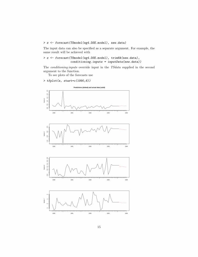
> z <- forecast(TSmodel(eg4.DSE.model), new.data)

The input data can also be specified as a separate argument. For example, thesame result will be achieved with

> z <- forecast(TSmodel(eg4.DSE.model), trimNA(new.data),

conditioning.inputs = inputData(new.data))

The conditioning.inputs override input in the TSdata supplied in the secondargument to the function.

To see plots of the forecasts use

> tfplot(z, start=c(1990,6))

Ser

ies

1

1990 1991 1992 1993 1994

0.0

0.5

1.0

1.5

2.0

2.5

Predictions (dotted) and actual data (solid)

Ser

ies

2

1990 1991 1992 1993 1994

−1.

0−

0.5

0.0

0.5

Ser

ies

6

1990 1991 1992 1993 1994

−0.

40.

00.

20.

40.

60.

8

Ser

ies

7

1990 1991 1992 1993 1994

−1

01

2

15

Sometimes a forecast for input data comes from another source, perhapsanother model. Rather than construct the conditioning.inputs as describedabove, another way to combine this forecast with the historical input data is touse the argument conditioning.inputs.forecasts:

> z <- forecast(eg4.DSE.model,

conditioning.inputs.forecasts = matrix(0.5,6,1))

This would use the input data from eg4.DSE.model and append 6 periods of 0.5to it.

Some generic functions which work with the structure returned by forecast :

> summary(z)

> print(z)

> tfplot(z)

> tfplot(z, start=c(1990,1))

If you actually want the numbers from the forecast they can be extracted with

> forecasts(z)[[1]]

The [[1]] indicates the first forecast (in this example there is only one, but thesame structures are used for other purposes discussed below. To see a subset ofthe data use tfwindow :

> tfwindow(forecasts(z)[[1]], start=c(1994,1), warn=FALSE)

This prints values starting in the first period of 1994.The horizon for the forecast is determined by the available input data (condi-

tioning.inputs or conditioning.inputs.forecasts). If neither of these are suppliedthen the argument horizon, which has a default value of 36, is used to repli-cate the last period of data to the indicated horizon. For models with no inputvariables the argument horizon controls the length of the forecast.

9 Evaluating Forecasting Models

How well does the model do at forecasting? The first thing to check is that modelforecasts actually track the data more or less. The generic function tfplot()works with results from the following functions. Recall that the function l()applies a TSmodel to TSdata and returns a TSestModel which includes one-stepahead forecasts. It can be used with any TSmodel and TSdata of correspondingdimension. So

> z <- l(TSmodel(eg4.DSE.model), new.data)

applies the previously estimated model to the new data, and

> tfplot(z)

16

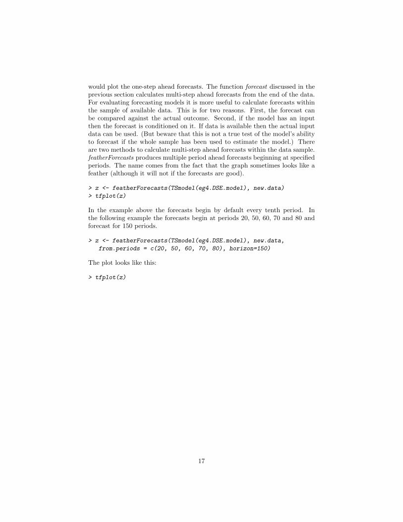
would plot the one-step ahead forecasts. The function forecast discussed in theprevious section calculates multi-step ahead forecasts from the end of the data.For evaluating forecasting models it is more useful to calculate forecasts withinthe sample of available data. This is for two reasons. First, the forecast canbe compared against the actual outcome. Second, if the model has an inputthen the forecast is conditioned on it. If data is available then the actual inputdata can be used. (But beware that this is not a true test of the model’s abilityto forecast if the whole sample has been used to estimate the model.) Thereare two methods to calculate multi-step ahead forecasts within the data sample.featherForecasts produces multiple period ahead forecasts beginning at specifiedperiods. The name comes from the fact that the graph sometimes looks like afeather (although it will not if the forecasts are good).

> z <- featherForecasts(TSmodel(eg4.DSE.model), new.data)

> tfplot(z)

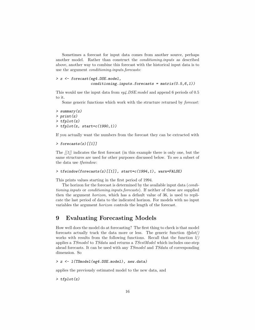
In the example above the forecasts begin by default every tenth period. Inthe following example the forecasts begin at periods 20, 50, 60, 70 and 80 andforecast for 150 periods.

> z <- featherForecasts(TSmodel(eg4.DSE.model), new.data,

from.periods = c(20, 50, 60, 70, 80), horizon=150)

The plot looks like this:

> tfplot(z)

17

Ser

ies

1

1974 1976 1978 1980 1982 1984 1986 1988 1990 1992 1994

0.0

0.5

1.0

1.5

2.0

2.5

Predictions (dotted) and actual data (solid)S

erie

s 2

1974 1976 1978 1980 1982 1984 1986 1988 1990 1992 1994

−1.

5−

0.5

0.5

1.0

1.5

2.0

Ser

ies

6

1974 1976 1978 1980 1982 1984 1986 1988 1990 1992 1994

−1.

0−

0.5

0.0

0.5

Ser

ies

7

1974 1976 1978 1980 1982 1984 1986 1988 1990 1992 1994

−2

−1

01

23

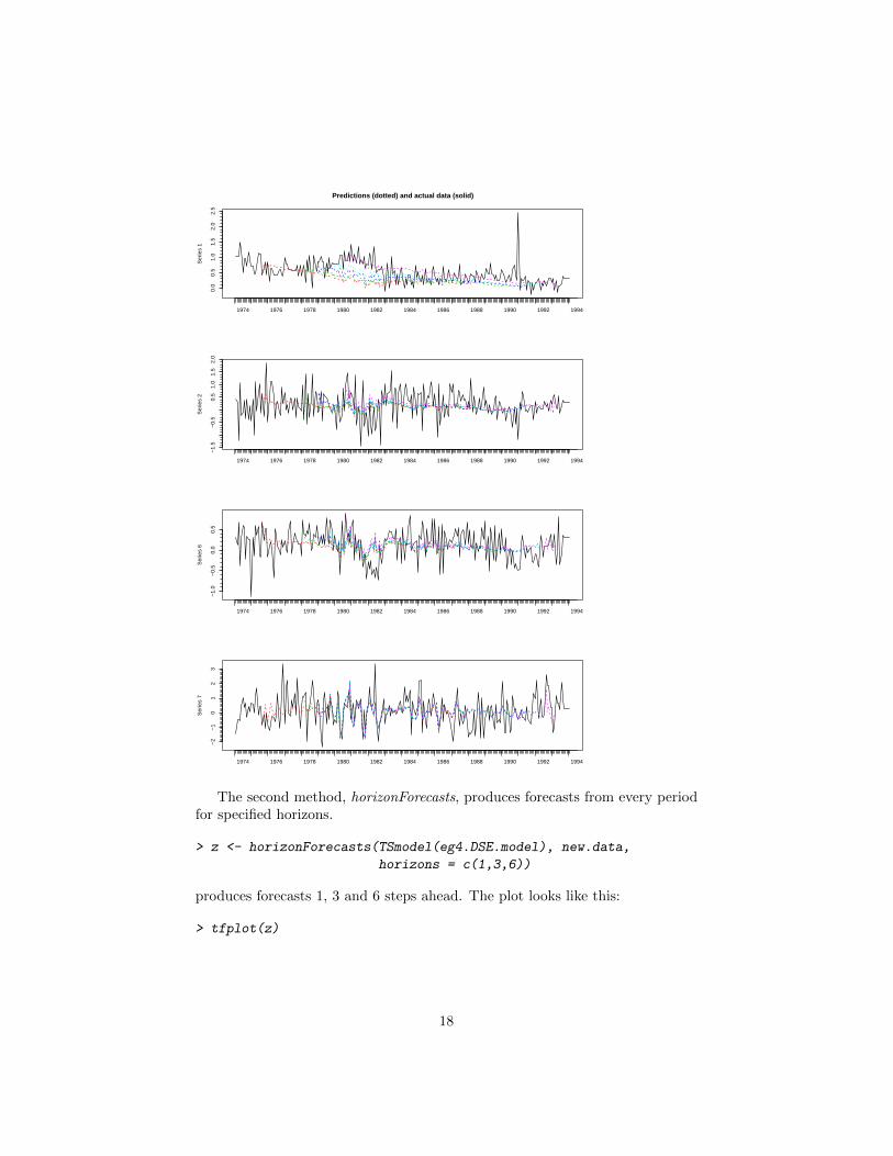
The second method, horizonForecasts, produces forecasts from every periodfor specified horizons.

> z <- horizonForecasts(TSmodel(eg4.DSE.model), new.data,

horizons = c(1,3,6))

produces forecasts 1, 3 and 6 steps ahead. The plot looks like this:

> tfplot(z)

18

Ser

ies

1

1974 1976 1978 1980 1982 1984 1986 1988 1990 1992 1994

0.0

0.5

1.0

1.5

2.0

2.5

Predictions (dotted) and actual data (solid)S

erie

s 2

1974 1976 1978 1980 1982 1984 1986 1988 1990 1992 1994

−1.

5−

0.5

0.5

1.0

1.5

2.0

Ser

ies

6

1974 1976 1978 1980 1982 1984 1986 1988 1990 1992 1994

−1.

0−

0.5

0.0

0.5

Ser

ies

7

1974 1976 1978 1980 1982 1984 1986 1988 1990 1992 1994

−2

−1

01

23

The result is aligned so that the forecast for a particular period is plottedagainst the actual outcome for that period. Thus, in the last example, the plotwill show the data for each period along with the forecast produced from 1, 3,and 6 periods prior. This plot is particularly useful for illustrating when modelsdo well and when they do not. A common experience with economic data isthat models do well during periods of expansion and contraction, but miss theturning points. The forecast covariance, to be discussed next, averages over allperiods. It is quite possible that a model can indicate turning points well butnot do so well on average, and thus be overlooked if only forecast covariance isconsidered. It is always useful to keep in mind the intended use of the model.

19

The numbers which generate the above plot can be extracted from the resultof horizonForecasts with forecasts(). This gives an array with the first dimen-sion corresponding to the horizons and the time frame aligned to correspond tothe data. So forecasts(z)[2,30,] from the above example will be the predictionmade for the 30th period from 3 periods previous (the second element indicatedin horizons is 3) and forecasts(z)[3,30,] will be the prediction made for the 30thperiod from 6 periods previous (horizons[3] is 6). Remember that these fore-casts are conditioned on the supplied input data, which means that the outputvariables here are forecast 1, 3 and 6 periods ahead, but true, not forecasted,input data is used.

If the forecasts look reasonable then examine the forecast errors more system-atically. The following calculates the forecast covariances at different horizons.

> fc <- forecastCov(TSmodel(eg4.DSE.model), data = eg4.DSE.data)

> tfplot(fc)

> tfplot(forecastCov(TSmodel(eg4.DSE.model), data = eg4.DSE.data,

horizons = 1:4))

The last example calculates for horizons from 1 to 4 rather than the default 1to 12. To see how the model forecasts relative to a zero forecast and a trendforecast:

> fc <- forecastCov(TSmodel(eg4.DSE.model), data = eg4.DSE.data,

zero = T, trend =T )

> tfplot(fc)

This is a very useful check (and often very humbling).You can also do out-of-sample forecast covariance analysis. This is discussed

in the EvalEst package vignette.There is not yet implemented in dse any measure of forecast errors which

can be compared across models - inevitably the covariance of the error is smallerfor less variable series and is also affected by scaling of the series. This may justmean that the series is easier to predict or has a different scale, not that theforecast equation is more brilliant. MAPE may be implemented sometime.

10 Adding New TSmodel Classes

dse uses object oriented methods for studying new estimation techniques andother kinds of time series models. Methods were implemented for studyingTroll (Intex Solutions, Inc.) models and some neural net architectures havealso been explored. These different model objects and estimation methods wereimplemented for research purposes. Users are encouraged to consider specificrepresentations used in this guide as examples in the context of dse’s broaderobjectives.

Models used in the package are of class TSmodel with secondary classes toindicate specific types of models. The distributed package supports subclass

20

ARMA and SS. The main methods which will be necessary for a new class ofmodels ”xxx” are print.xxx, is.xxx, l.xxx, simulate.xxx, seriesNamesInput.xxx, se-riesNamesOutput.xxx, checkConsistentDimensions.xxx, and MonteCarloSimula-tions.xxx. Also, the method to.xxx is useful for converting models from existingclasses to this new class where possible. Models should inherit from TSmodel.

11 Adding New TSdata Classes

Data used by functions in this package are objects of class TSdata. The defaultmethods assume that this is a list with an element output and optionally anelement input, each of which is a (multivariate) time series object. New classesof time series can be defined and the dse package should work as long as themethods describe in the tframe package are implemented for the new time seriesclass. This usually will not require any changes to TSdata methods (or anythingelse in the dse package).

21

12 Appendix I: Mini-Reference

Following is a short list of some of the functions. The online help contains moredetails on all functions, while the guides for each package contain more completedescriptions.

OBJECTS

� ARMA - define an ARMA TSmodel

� SS - define a state-space TSmodel

� TSdata - an input/output time series data structure

� TSestModel - a TSmodel estimated with TSdata

MODEL INFORMATION

� print - display model arrays

� summary - summary information about a model

� tfplot - plot data or model predictions.

MODEL PROPERTIES

� McMillan.degree - calculate the McMillan degree of a model

� roots - calculate the roots of a model

� stability - check stability of model

MODEL CONVERSION

� to.SS - convert to an equivalent state space innovations representation

� to.ARMA - convert to an ARMA representation

SIMULATION, ONE-STEP PREDICTIONS & RELATED STATIS-TICS

� simulate - Simulate a model to generate artificial data.

� l - evaluate a TSmodel with TSdata and return a TSestModel object

� smoother - calculate smoothed state for a state space model.

� check.residuals - distribution, autocorrelation and partial autocorrelationof residuals

� information.tests - print model selection criteria

22

MODEL ESTIMATION & REDUCTION

� est.VARX.ls - estimate VAR model with exogenous variable using OLS

� est.VARX.ar - estimate VAR model with exogenous variable using auto-correlations

� est.SS.from.VARX - estimate a VARX model and convert to state space

� est.SS.Mittnik - estimate state space model using Mittnik’s markov pa-rameter technique

� estMaxLik - Maximum likelihood estimation of models.

� est.black.box - estimate and find the best reduced model

� bft - estimate and find the best reduced model by techniques in Gilbert(1995), also referred to as est.black.box4

� reduction.Mittnik - nested-balanced state space model reduction by svd ofHankel generated from a model

FORECAST AND FORECAST EVALUATION

� forecast - generate a forecast from given model and data.

� featherForecasts - forecast from specified periods

� horizonsForecasts - forecast specified periods ahead

� forecastCov - calculate covariance of multi-period ahead forecasts

23