Embed Size (px)
Citation preview

Broadband aggregation in therural areas of Denmark
Master thesis
Jais Langkow Kristensen
Aalborg UniversityElectronics and IT

Department of Electronic Systems
Aalborg University
http://www.aau.dk
Title:Broadband aggregation in the rural ar-eas of Denmark
Theme:Master’s thesis
Project Period:Fall Semester 2015 - Spring Semester2016
Project Group:1021
Participant(s):Jais Langkow Kristensen
Supervisor(s):Tatiana MadsenThomas JacobsenAndrea Fabio Cattoni
Copies: 2
Page Numbers: 45
Date of Completion:June 2, 2016
Abstract:
This work presents a solution for ag-gregating multiple connections, in or-der to utilise the throughput of bothsimultaneously. This system is us-ing the routing tables in Linux to setthe default routes for each flow. Theflows are being split based on weights,which are determined by the perfor-mance of each connection. The met-ric used in this work to evaluate theperformance is the congestion window(CWND). The CWND is propagatedfrom the client to the router via scp,and the router uses this informationto determine the weights. The systemperformance was tested. The resultsfrom the tests shows that an increasein throughput can be achieved whenutilising two connections compared tousing one connection. The test alsoshowed that the system does not im-prove the throughput, compared to asystem with intelligent splitting dis-abled.
The content of this report is freely available, but publication (with reference) may only be pursued due to
agreement with the author.

Contents
Preface v
1 Introduction 31.1 Coverage . . . . . . . . . . . . . . . . . . . . . . . . . . . . . . . . . . . 3
1.1.1 Measurement results . . . . . . . . . . . . . . . . . . . . . . . . 31.2 Bandwidth aggregation . . . . . . . . . . . . . . . . . . . . . . . . . . 41.3 Service awareness . . . . . . . . . . . . . . . . . . . . . . . . . . . . . . 51.4 Commercial products . . . . . . . . . . . . . . . . . . . . . . . . . . . . 51.5 Problem statement . . . . . . . . . . . . . . . . . . . . . . . . . . . . . 6
2 Initial analysis 72.1 System architecture . . . . . . . . . . . . . . . . . . . . . . . . . . . . . 72.2 Test specification . . . . . . . . . . . . . . . . . . . . . . . . . . . . . . 9
3 Design 113.1 Routing method . . . . . . . . . . . . . . . . . . . . . . . . . . . . . . . 11
3.1.1 Multipath TCP . . . . . . . . . . . . . . . . . . . . . . . . . . . 113.1.2 Hybrid architecture . . . . . . . . . . . . . . . . . . . . . . . . 123.1.3 Routing tables . . . . . . . . . . . . . . . . . . . . . . . . . . . . 12
3.2 Performance measurement . . . . . . . . . . . . . . . . . . . . . . . . 133.2.1 Passive performance measurement . . . . . . . . . . . . . . . 133.2.2 Active performance measurement . . . . . . . . . . . . . . . . 14
3.3 Calculating the CWND . . . . . . . . . . . . . . . . . . . . . . . . . . . 163.4 Algorithm design . . . . . . . . . . . . . . . . . . . . . . . . . . . . . . 16
4 Implementation 194.1 Splitting the traffic . . . . . . . . . . . . . . . . . . . . . . . . . . . . . 194.2 Propagating congestion window from client to router . . . . . . . . . 204.3 Receiving the congestion window . . . . . . . . . . . . . . . . . . . . 214.4 Calculating the weights . . . . . . . . . . . . . . . . . . . . . . . . . . 22
iii

iv Contents
5 Test 255.1 Test script . . . . . . . . . . . . . . . . . . . . . . . . . . . . . . . . . . 255.2 Test results . . . . . . . . . . . . . . . . . . . . . . . . . . . . . . . . . . 26
6 Conclusion 336.1 Conclusion . . . . . . . . . . . . . . . . . . . . . . . . . . . . . . . . . . 336.2 Future work . . . . . . . . . . . . . . . . . . . . . . . . . . . . . . . . . 34
Bibliography 35
A Create tables 37
B Test results 39B.1 Single connection limited to 2 mbps . . . . . . . . . . . . . . . . . . . 39B.2 Single connection limited to 6 mbps . . . . . . . . . . . . . . . . . . . 41B.3 Two connections no intelligence . . . . . . . . . . . . . . . . . . . . . 41B.4 Two connections with intelligence . . . . . . . . . . . . . . . . . . . . 41B.5 Single connection limited to 4 mbps . . . . . . . . . . . . . . . . . . . 41
Acronyms
ACK Acknowledgement
ADSL Asymmetric Digital Subscriber Line
AIMD Additive Increase/Multiplicative Decrease
CWND Congestion Window
FSM Finite-State Machine
GRE Generic Routing Encapsulation
HYA HYbrid Access
ISP Internet Service Provider
MPTCP MultiPath TCP
NAT Network Address Translation
QoS Quality of Service
RTT RoundTrip Time
ToS Type of Service
VPN Virtual Private Network

Preface
This report documents a master thesis project, for the Networks and DistributedSystems programme at the Department of Electronic Systems, Aalborg University.
The code used in this project is uploaded on digital exam, and can also befound on:http://kom.aau.dk/group/16gr1021/Code/The code on the client is located in the folder called Client. This folder containsfour scripts
PPropCWND.sh Propagates the congestion window from client to router.
SleepClientsDuo.sh Runs the tests.
tcpshoot.c Used for file transfer in the tests.
tcpsnoop.h Used for file transfer in the tests.
The code on the router is located in the folder called Router. This folder con-tains four scripts
CreateTables.sh Creates the routing tables.
SetupVars.sh Sets the variables.
iftest.sh Assigns the new weights.
multiarraytest.py Calculates the weights.
Acknowledgement
The author would like to thank Aamir Saeed for technical sparring and cooperationwhile writing this report.
Aalborg University, June 2, 2016
v

Preface 1
Abstract
The internet connection in the rural areas of Denmark are lacking throughput andoften have very poor latency. This causes the farms to have inefficient productionand the families to have limited access to certain services like video streaming andVoIP. In order to overcome these issues, more connections could be utilised.
This solution is provided by a number of services, which all have some disad-vantages, but split the traffic on the available connections.
The splitting can be done in numerous ways, and on multiple levels in the OSImodel. In this report the traffic splitting will be done on the transport layer. In or-der to determine how the traffic should be split on the connections, an intelligentalgorithm is required. This report suggests using the performance of the connec-tions, to determine how much traffic should be routed on each connection. Theperformance metric used in this report is the CWND.The system presented in this report consists of two entities; the client and therouter. The client generates traffic, by visiting websites and transferring files viaFTP. Further the client device propagates the CWND of all the current flows to therouter regularly. This transmission is necessary, since only the sender knows theCWND value. Another solution could be to estimate the CWND on the router byobserving the traffic and adjusting the CWND accordingly.The router entity in the system splits the traffic flows on each connection accordingto some weights. These weights are adjusted dynamically using the CWND.


Chapter 1
Introduction
A reliable and fast Internet connection is one of the cornerstones in a modern society. Accessto up-to-date Internet speed is necessary for any household and business to achieve fullpotential of the digital opportunities. This report will cover the current Internet speed andreliability in rural Denmark, and propose solutions to improve the bandwidth. This chapterintroduces and motivates the problem of bandwidth aggregation. The problem statement isdefined in the end of the chapter.
1.1 Coverage
The broadband coverage in Denmark is in general good. However as Figure 1.1shows, there are parts where 100 mbps download is not achievable. Further, themap estimates where the infrastructure supports the speed, and not whether ornot the speed is supplied.
In order to find the actual speeds of the Asymmetric Digital Subscriber Line(ADSL) line an the LTE connection, measurements have been performed in twolocations in northern Jutland, specifically at a farm in Tylstrup (farm 1) and one inSæby (farm 2). These measurements were taken over the course of one week.
The following section will cover some of the results from these measurements.Further results can be seen in [2].
1.1.1 Measurement results
This section contains the figures produced from the measurements.Figure 1.2 shows the throughput measured at the first farm located in Tylstrup.
The ethernet cable bars represent the throughput of the deployed ADSL line. TheLTE bars represent the throughput measured directly from the LTE antenna. TheWiFi bars represent the throughput measured outside and inside the farm house.
3

4 Chapter 1. Introduction
Figure 1.1: Coverage map of Denmark [3]
Figure 1.2: Measurements from the farm in Tylstrup.
As Figure 1.2, Figure 1.3 shows the measured throughput. The ADSL connec-tion is better on this farm than in farm 1, but it is still in the lower end of internetspeeds.
1.2 Bandwidth aggregation
Since the ADSL and LTE connection in rural areas in Denmark are either slow orunreliable in coverage (as described in section 1.1 and 1.1.1), a single connection

1.3. Service awareness 5
Figure 1.3: Measurements from the farm in Sæby.
can not support the requirements of a modern family and small business. Thisissue might be solved by aggregating the LTE connection and the xdsl connection,and simply summing the data rates. An example of this is shown in figure 1.4.
Figure 1.4: This figure illustrates the basic concept of bandwidth aggregation. Each line between thetwo boxes represent different connections with different data rates.
1.3 Service awareness
When aggregating bandwidth, multiple methods can be thought of. One methodcould be to blindly treat all traffic equally and separate the packets on the variousconnections. Another method could be to divide the traffic into services and prior-itize different services differently depending on the Quality of Service (QoS) thatservice needs. This method can improve the experience of services that requirehigh data rates, while still giving the same experience of services that does notrequire as high data rates such as e-mail.
1.4 Commercial products
Multiple solutions providing bandwidth aggregation exists on the market already,however these have some restrictions in usability or are quite expensive. This

6 Chapter 1. Introduction
section will cover some of these.
Speedify Speedify is a service that utilises channel bonding to aggregate connec-tions. The solution is patented in [1], but does not cover how the load balancingis done and does not allow for configuration thereof. The Speedify solution workswithout any additional hardware, only a piece of software is required. It is afreemium service, where one can get a free packet which includes 1 GB of data permonth, a 50 GB data plan that costs 9 $ per month and finally an unlimited dataplan that costs 12 $ per month.
Viprinet Viprinet functions, like Speedify, by utilising a multichannel Virtual Pri-vate Network (VPN) router and channel bonding as seen in Figure 1.5. In thisexample the data stream from the user is encrypted and distributed on the variousInternet connections. The split data packets are transmitted through the InternetService Providers (ISPs) and reaches the data center, which decrypts, aggregatesand forwards the data to the destination [13]. In this setup, a device is neededfrom Viprinet, either a multichannel VPN router or hub. This of course increasesthe cost of this service.
Figure 1.5: An example of the Viprinet setup
Viprinet is by far the most expensive solution with prices up to 11990 GBP [12].
1.5 Problem statement
How can a system that aggregates multiple connections, intelligently bedeveloped and implemented.
This report will focus on improving the speed of the connection rather thanfocusing on reliability. However it is expected that a fairly high reliability will bea natural consequence of utilising more connections with the TCP protocol. Thefollowing chapter will describe how a system, that solves the problem statement,could look.

Chapter 2
Initial analysis
This chapter serves as an initial exploration of the problem statement. First theoverall system architecture will be described and analysed. Given this analysis atest specification will be stated. This specification will be used in chapter 5 in orderto thoroughly test the system.
2.1 System architecture
In order to develop the system described in section 1.5, an overall systemarchitecture have been formulated and visualised in figure 2.1. Each sub-system will be described in the following sections.
Figure 2.1: This figure illustrates how the overall system should look.
The system consists of the following subsystems: The tunnels and Aggregation
server is only required in some routing methods. These will be describedin a later chapter.
7

8 Chapter 2. Initial analysis
The following sections will be describing the sub systems shown in Fig-ure 2.1, and further explain why they are needed.
Packet classification
In order to divide the traffic according to the Type of Service (ToS), asdescribed in section 1.3, a classifier is required. The classifier should beable to determine the ToS affiliated with the packet or flow.
Performance of connections
When dividing the traffic intelligently, the performance of each connectionneeds to be measured. This way the link with the best performance can getthe most traffic compared to the link with the worst performance.
Routing method
This is the main subsystem in the overall system. In this block the packetsare routed on the available links. This block also decides how the aggrega-tion server is going to be designed, as these are inherently linked.
Routing algorithm
In order to split the traffic intelligently, a routing algorithm is needed. Thisalgorithm utilises the functionalities of the routing method and the perfor-mance of each connection, and assigns the packet to the optimal link.
Tunnels
As some services, such as https [6], require a unique IP pair, tunnels arerequired. These have the purpose of tunneling the traffic to a single server,which then forwards the traffic with one IP pair per flow to the final desti-nation.
Aggregation server
The purpose of the aggregation server is to aggregate the traffic after thesplitting. It also serves as the proxy for the tunnels.
Due to time limitations, this report will not take the ToS into accountwhen splitting the traffic. Due to this limitation, an updated system overviewfigure is presented in Figure 2.2

2.2. Test specification 9
Figure 2.2: This figure illustrates how the overall system should look after limitations.
2.2 Test specification
In this section a test specification will be stated. The purpose of the testsspecified is to verify that the system behaves as expected and to measurethe performance in terms of throughput.In the test setup two connections will be used: One LTE subscription fromTelenor and the wired internet at AAU. These will be limited to mimicthe throughput, that can be expected in the rural areas of Denmark. Thelimits will be 2 and 4 mbps. The tool used to limit the connections iswondershaper. This tool uses the iproute’s tc command to control the trans-mission rate. During each test, some traffic will be generated.
Test 1
In this test one link will be used. This link will be limited to 2 mbps. Thepurpose of this test is to set a minimum throughput.
Test 2
In this test one link will be used. This link will be limited to 6 mbps. Thepurpose of this test is to set an upper bound of what can be achieved.
Test 3
In this test two links will be used limited at 2 and 4 mbps accordingly. Inthis test the routing algorithm described above will be disabled. The pur-pose of this test is to verify that an increase in throughput can be achievedwhen applying the intelligent routing algorithm.

10 Chapter 2. Initial analysis
Test 4
As in test 3, this test will be carried out on two connections limited to 2 and4 mbps. In this test the routing algorithm is enabled. The purpose of thistest is, as in test 3, to verify that an increase in throughput can be achieved.
In this chapter the overall system architecture was presented and analysed. Thisanalysis lead to some limitations to the problem. In addition to this a test specifica-tion was defined in section 2.2.

Chapter 3
Design
Given the limitations specified in chapter 2 the system will be analysed. In thisanalysis the state of the art of each subsystem will be presented. Further the algo-rithms needed in each subsystem will be developed.
3.1 Routing method
In this section the state-of-the-art technologies and methods will be de-scribed. This will lead to a design decision.
3.1.1 Multipath TCP
MultiPath TCP (MPTCP) [5] provides simultaneous use of more than onepath between hosts, with all the features of a normal TCP connection.MPTCP enables the hosts to use different paths with different IP addressesto exchange packets. The MPTCP connection appears as a normal TCPconnection to the application, and each subflow in the MPTCP looks likea regular TCP connnection, with the only difference of some TCP options.MPTCP manages the initialisation, termination and utilisation of the sub-flows. MPTCP is currently being used commercially by smartphone man-ufacturers and companies providing routing equipment with the sole pur-pose of combining connections [4].
Advantages MPTCP provides the same inherent features as standard TCP,which makes the communication reliable.
Disdvantages Since this technology is distributing packets over multipleIP addresses, some applications like https that require a secure connec-
11

12 Chapter 3. Design
tion, will fail to function [6]. This issue can be solved using a VPN tunnel.MPTCP is not yet standardised and is still experimental.
3.1.2 Hybrid architecture
The HYbrid Access (HYA), presented in [9], enhances the overall through-put, by aggregating the bandwidth from a LTE and DSL connection througha Generic Routing Encapsulation (GRE) tunnel. The data rate and RoundTripTime (RTT) of a DSL link is mostly constant, while the data rate and RTT onLTE varies over time depending on the number of users in the cell. In HYA,the packet reorder buffer size is related to the difference in RTT on the twolinks used. A large RTT difference leads to a lower bandwidth efficiency.The maximum RTT the customer will experience is the larger of the twolinks. HYA uses one connection first, when this is saturated, the other linkwill be used. This benefits customers with different prices on each link.
Advantages Since the HYA uses the cheapest link until this is saturated,the overall price for the customer will be minimized.
Disdvantages Needs an aggregation/proxy server in order to combine andreorder the packets, and ensure a single IP pair.
3.1.3 Routing tables
In order to utilise more connections, the routing tables in Linux can be used.[11] presents a method to maintain more default routes for the different in-coming flows.A packet arrives from the local network and the Network Address Transla-tion (NAT) searches already existing connections to determine whether it isa new connection. When the gateway encounters a new connection, it cre-ates an uninitialised info-block and passes the packet to the routing system.In the routing system, the kernel uses some predefined weights, to extracta default route from the multipath default routes. This provides the outputinterface and IP address of the next gateway and thereby enabling routingfor this flow. The packet then passes the postrouting chain in the NAT ta-ble.A second packet arrives from the local network with same IP pair as theprevious packet. It passes through the prerouting chain of the mangle ta-ble. Since it has the same IP pair, the NAT roues it to the same outputinterface as was assigned earlier.

3.2. Performance measurement 13
Advantages This method does not require any external equipment, such asaggregation or proxy servers, since it operates per flow.
Disdvantages Since this method operates per flow, a number of unique IPpairs is required for the method to split the traffic.
Design choice
In this report the method described in section 3.1.3 will be used. The rea-son for this is that it does not require any aggregation of the packets, andtherefore can be implemented using only a router. This design choice givesa new system overview figure, which is presented in Figure 3.1
Figure 3.1: This figure illustrates how the system will look
3.2 Performance measurement
In order to route the traffic intelligently, knowledge of the condition ofthe connections is required. This knowledge can be obtained actively orpassively. This section will be describing the difference between these two,and their advantages and disadvantages.
3.2.1 Passive performance measurement
When doing passive measurements, the traffic going through the link isbeing observed. From these observations the current state of the link can beestimated. This estimation can be based on various metrics, some of thesewill be described here. Common for all these methods is that they onlywork when traffic is transmitted.

14 Chapter 3. Design
Round trip time
The RTT can be estimated by measuring the time from a packet is send tothe Acknowledgement (ACK) is received.
Bandwidth
The bandwidth can be estimated by counting the number of bytes leavingthe link each second.
Congestion window
The congestion window tells how congested the link is. If the Conges-tion Window (CWND) is decreasing, the link is congested, however if theCWND is increasing or not changing, the link has ’room’ for more traf-fic. The CWND is calculated using Additive Increase/Multiplicative De-crease (AIMD). This algorithm varies through the implementaions of TCP.
3.2.2 Active performance measurement
When doing active measurements, the link is being probed with data pack-ets of a certain size. Due to the probing, extra traffic is transmitted on thelink, which could reduce the performance of the actual traffic being trans-mitted, and may cause a higher cost for the subscriber. Many methodsexists for doing active measurements, some of these will be described here.
Packet pair
The packet pair method estimates the bottleneck link bandwidth. This isdone by sending two packets from the same source to the same destination.(3.1) shows how the bandwidth is calculated [8].
t1n − t0
n = max(
s1
b1, t1
0 − t10
)(3.1)

3.2. Performance measurement 15
t0n Arrival time of the first
packet[s]
t1n Arrival time of the second
packet[s]
t00 Transmission time of the
first packet[s]
t10 Transmission time of the
second packet[s]
s1 Size of the second packet [b]b1 bandwidth of the bottle-
neck link[bps]
Advantages Simple to implement and does not introduce a lot of extratraffic on the link.
Disdvantages Very vulnerable to cross traffic.
Train of packets
The train of packet method was introduced in [7]. In the method the sourcesends a ’train’ of packets to a destination node. The bandwidth is calculatedusing (3.2)
bw =
((n− 1) ∗ s
∑ IaT
)(3.2)
bw Bandwidth [bps]n Number of packets [·]s Size of packets [b]IaT Inter arrival time [s]
Advantages Simple to implement and does not introduce a lot of extratraffic on the link.
Disdvantages Very vulnerable to cross traffic.
Other methods exist but will not be discussed in this report.In this project the method described in section3.2.1 will be used.

16 Chapter 3. Design
Another possible solution for getting the CWND on the router is to cal-culate it directly there. The work presented in [10], shows how the CWNDcan be calculated using Finite-State Machine (FSM). The following sectionwill describe the method they use.
3.3 Calculating the CWND
As described in section 3.2.1 the CWND is calculated using the AIMD. Thiscan be done at any point on the route from sender to receiver, if it is as-sumed that all ACKs from receiver to sender are received at the sender. Theidea is to create a duplicate of the senders state for each flow. This is doneby observing the traffic in both directions between sender and receiver. ATCP sender can be in either slow-start or congestion avoidance mode. Foreach ACK received the CWND is either increased by 1 or 1/CWND. Inthe case where loss is detected by receiving 3 duplicate ACKs, each TCPflavor acts differently. In [10] the 3 most common TCP flavors are consid-ered, namely Tahoe, Reno and NewReno. These are distinguished by usingthe fact that any TCP sender cannot have more unacknowledged packetsthan min(cwnd, acwnd1). This fact is utilised by checking each packet sent,if it violates any of the flavors. The flavor with the least violations, is theflavor of this flow.
3.4 Algorithm design
In order to determine the weights in the kernel, an algorithm is required.In this section this algorithm will be designed.
In order to set the weights, the state of the connection is used.
if StateO f Connectionx == bad thenif Wx ≥ 2 then
Wx ←Wx − 1end if
elseWx ←Wx + 1
end ifThis way the weights will decrease if the connection is bad and increase
else. A weight of zero would mean that no traffic is directed on that connec-1the receivers advertised window

3.4. Algorithm design 17
tion. This is an undesirable situation, and is avoided by checking Wx ≥ 2.The StateO f Connectionx can be found in multiple ways. All of these meth-ods require the change in CWND to be found. This is, in this report, definedin (3.3).
∆CWNDyx = CWNDy
x(t− τ)− CWNDyx(t) (3.3)
y Flow number [·]x Connection [·]CWNDy
x Congestion window size [Byte]t time [seconds]τ time interval [seconds]
The StateO f Connectionx can be either ’bad’ or ’good’. Some of the waysto determine this will be described in the following algorithms.
Algorithm 3.1 Using the first flow only
if ∆CWND1x ≤ 0 then
StateO f Connectionx ← goodelse
StateO f Connectionx ← badend if
This algorithm only looks at the first flow, when deciding whether thelink should be marked as good or bad. The disadvantage of this method isthat if the flow closes, the algorithm compares the now closed flow CWNDwith a different flow CWND. This situation can be avoided by taking theaverage CWND of all the flows.
Algorithm 3.2 Using the the average CWND, Y is the number of flows
λ(∆CWNDyx) =
Y∑
i=1∆CWNDi
x
Yif λ(∆CWNDy
x) ≤ 0 thenStateO f Connectionx ← good
elseStateO f Connectionx ← bad
end if

18 Chapter 3. Design
The disadvantage of taking the mean of the CWNDs, is that if one flowis being saturated, and is increased while another flow is not saturated yet,the mean will show that the CWND is constant, labelling the link as being’good’. The next algorithm may solve this issue.
Algorithm 3.3 Majority ruling, Y is the number of flows
GoodFlows = 0BadFlows = 0for i=1; i<=Y; i++ do
if ∆CWNDix ≤ 0 then
GoodFlows← GoodFlows + 1else
BadFlows← BadFlows + 1end if
end forif GoodFlows ≥ BadFlows then
StateO f Connectionx ← goodelse
StateO f Connectionx ← badend if
Other methods exists, but will not be described in this report. Due totime constraints, Algorithm 3.1 will be used for determining the state of theconnections in this report.
In this chapter the system was analysed. Given this analysis some additionallimitations were introduced. The analysis and limitations led to the design of thesystem and the underlying subsystems. Further the concept of weights was intro-duced as the way to split the traffic flows. These weights are being determined inAlgorithm 3.1. In the following chapter the implementation of the system will bedescribed.
Chapter 4
Implementation
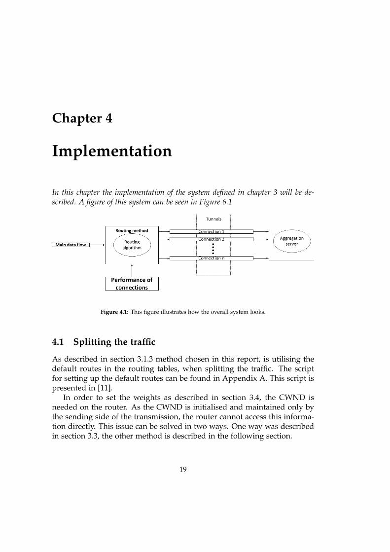
In this chapter the implementation of the system defined in chapter 3 will be de-scribed. A figure of this system can be seen in Figure 6.1
Figure 4.1: This figure illustrates how the overall system looks.
4.1 Splitting the traffic
As described in section 3.1.3 method chosen in this report, is utilising thedefault routes in the routing tables, when splitting the traffic. The scriptfor setting up the default routes can be found in Appendix A. This script ispresented in [11].
In order to set the weights as described in section 3.4, the CWND isneeded on the router. As the CWND is initialised and maintained only bythe sending side of the transmission, the router cannot access this informa-tion directly. This issue can be solved in two ways. One way was describedin section 3.3, the other method is described in the following section.
19

20 Chapter 4. Implementation
4.2 Propagating congestion window from client to router
Since only the sender knows the CWND, and the router needs this informa-tion, to set the weights in the load balancing system, one solution could beto propagate the value from the client to the router. This is done in Listing4.1.
Listing 4.1: Obtaining and propagating the CWND.
1 #!/bin/bash
2 while true
3 do
4 # Obtaining socket statistics and saving in ssfile.dat
5 ss -itn4 > ssfile.dat
6 # Clear old file
7 > cwndfile.dat
8 # Remove header from ssfile
9 tail -n +2 ssfile.dat > ssNew.dat
10 lines=$(cat ssNew.dat | wc -l)
11 # Getting every second line in ssNew.dat
12 for ((i=1; i<= $lines; i=i+2))
13 do
14 let o=$i+1
15 # Removing unnecessary text from line 1, 3, 5...
16 # In order to get the IP DST address
17 awk 'NR=='$i '' ssNew.dat | awk 'print $5' | grep
'[0 -9]\1 ,3\\.[0 -9]\1 ,3\\.[0 -9]\1 ,3\\.[0 -9]\1 ,3\ ' | sed s
/:[0 -9]*//g >> tmp.dat
18 # Removing unnecessary text from line 2, 4, 6...
19 # In order to get the CWND
20 awk 'NR=='$o '' ssNew.dat | awk ' print $1 $2 $3 $4 $5 $6 $7 $8 ' |
grep -Po 'cwnd :[0-9]*' | sed s/cwnd ://g >> tmp.dat
21 tmpLines=$(cat tmp.dat | wc -l)
22 # If the flow has a CWND
23 if (( $tmpLines ==2))
24 then
25 # Add IP and cwnd to cwndfile.dat
26 cat tmp.dat >> cwndfile.dat
27 fi
28 # Clear tmp file
29 > tmp.dat
30 done
31 # Transfer file to the router
32 scp cwndfile.dat sabwa@10 .0.0.1:/ home/sabwa/RoutingTables
33 # Append to Result file , for plotting purposes
34 cat cwndfile.dat >> cwndResult.dat
35 sleep 1
36 done
In Listing 4.1, the ss command is used to get information on all existingflows. This information is shaped into a usable format, and propagated us-ing scp. The information is also stored in the file cwndResult.dat, for testingand plotting purposes. The transmitted file has the following format:

4.3. Receiving the congestion window 21
Listing 4.2: cwndfile.dat format
1 216.58.209.142
2 12
3 216.58.209.131
4 10
5 109.105.109.207
6 10
7 216.58.209.142
8 10
When the router has received the file, it initiates the performance estimationof each link as described in 3.4.
4.3 Receiving the congestion window
While the script described in section 4.2, is running, the router needs a wayto convert the IP’s to the associated interfaces and calculate the weightsfrom the received CWNDs. This is done in Listing 4.3.
Listing 4.3: Get cwndfile.dat
1 #!/bin/bash
2 . SetupVars.sh
3 ./ CreateTables.sh
4 # Available interfaces
5 interList =(eth0 eth3)
6 # Initial weights
7 weightlist =(1 1)
8 # Initial CWND
9 oldcwnd =(10 10)
10 len=$#interList[@]
1112 while true
13 do
14 # If file has been received
15 if [ -e "cwndfile.dat" ]
16 then
17 # Initialise arrays
18 cwnd =()
19 inter =()
20 lines=$(cat cwndfile.dat | wc -l)
21 filecontent =(`cat cwndfile.dat `)
22 let lines=$lines -1
23 for i in $(seq 0 $lines)
24 do
25 if (($i % 2 ==0))
26 then
27 # Append interface name to array
28 inter +=($(ip route get $filecontent[$i] | awk ' print $5'
| head -n1))
29 else
30 # Append CWND to array
31 cwnd +=($filecontent[$i])
32 fi

22 Chapter 4. Implementation
33 done
34 leninter=$#inter[@]
35 len2=$#cwnd[@]
36 # For testing data
37 echo $inter[@] >> ./ Actualtests/FlowsFive2MultiPlus.txt
38 echo $cwnd[@] >> ./ Actualtests/FlowsFive2MultiPlus.txt
39 # Python script to calculate the weights
40 python multiarraytest.py $len $interList[@] $weightlist[@] $
oldcwnd[@] $len2 $inter[@] $cwnd[@] > temp.txt
The last line in Listing 4.3 calls a python script. The following sectionwill describe this script.
4.4 Calculating the weights
The first 32 lines in the python script, loads the variables from the bashscript. Since the variables from the bash script are in arrays, the pythonscript needs to load these one element at the time. Listing 4.4 shows anexample of how the variables are loaded.
Listing 4.4: Calculating the weights
10 # Load variables to list
11 for i in range(lengh):
12 interList [(i)] = str(sys.argv[(i+2)])
13 o += 1
14 for i in range(lengh):
15 weightList [(i)] = int(sys.argv[(i+lengh +2)])
16 o += 1
17 for i in range(lengh):
18 oldCwnd [(i)] = int(sys.argv[(i+lengh +4)])
19 o += 1
Once the variables are loaded, the weights are calculated and printed tothe bash script to set the new weights. Listing 4.5 shows this.
Listing 4.5: Calculating the weights
34 # For no of flows
35 for k,item in enumerate(inter):
36 # Is interface registered
37 if inter[k] in TotList [0]:
38 indexx = TotList [0]. index(inter[k])
39 # If interface is not set and oldcwnd <= current cwnd
40 if TotList [3][ indexx ]==0 and TotList [2][ indexx]<=cwnd[k]:
41 newcwnd[indexx] = cwnd[k] # Set new to current
42 TotList [3][ indexx] = 1 # Interface set
43 TotList [1][ indexx] += 1 # Add 1 to weight
44 # If interface is not set and oldcwnd > current cwnd
45 elif TotList [3][ indexx ]==0 and TotList [2][ indexx]>cwnd[k]:
46 TotList [3][ indexx] = 1 # Interface set

4.4. Calculating the weights 23
47 newcwnd[indexx] = cwnd[k] # Set new to current
48 # Is weight >= 2
49 if TotList [1][ indexx ]>=2:
50 TotList [1][ indexx] -= 1 # subtract 1 from weight
5152 for k,item in enumerate(interList):
53 # If interface is not set (no flows on interface)
54 if TotList [3][k]==0:
55 TotList [1][k] +=1 # Add 1 to weight
5657 # Reducing the fraction
58 f=Fraction(TotList [1][0] , TotList [1][1])
59 TotList [1][0]=f.numerator
60 TotList [1][1]=f.denominator
61 weightList [0]=f.numerator
62 weightList [1]=f.denominator
63 # Design choice , one weight may not be more than 5 times the other weight
64 if (weightList [0]- weightList [1]) >=5:
65 weightList [0]= weightList [0]-1
66 elif (weightList [1]- weightList [0]) >=5:
67 weightList [1]= weightList [1]-1
68 # Output
69 print(newcwnd)
70 print(weightList)
After the python script is done, the bash script updates the routing tablewith the newly calculated weights. This can be seen in Listing 4.6.
Listing 4.6: Get cwndfile.dat
41 # Output from python script
42 Alloldcwnd=$(cat temp.txt | head -n1 | sed 's/[][]//g' | sed s/,//g)
43 Allweightlist=$(cat temp.txt | tail -n +2 | sed 's/[][]//g' | sed s
/,//g)
44 # Updating the variables
45 oldcwnd [0]=$(echo $Alloldcwnd | awk ' print $1')
46 oldcwnd [1]=$(echo $Alloldcwnd | awk ' print $2')
47 weightlist [0]=$(echo $Allweightlist | awk ' print $1')
48 weightlist [1]=$(echo $Allweightlist | awk ' print $2')
49 # Setting the weights
50 Weight1=$(echo $Allweightlist | awk ' print $1')
51 Weight2=$(echo $Allweightlist | awk ' print $2')
52 # For testing data
53 echo $interList[@] >> ./ Actualtests/Five2sMultiPlus.txt
54 echo $Alloldcwnd[@] >> ./ Actualtests/Five2sMultiPlus.txt
55 echo $Allweightlist[@] >> ./ Actualtests/Five2sMultiPlus.txt
5657 rm cwndfile.dat
58 # Update routing tables with new weights
59 ./ CreateTables.sh
60 else
61 # Just to verify the script is running :-)
62 echo "No file"
63 sleep 1
64 fi
65 done

24 Chapter 4. Implementation
In this chapter the system overview figure was presented, and the implementa-tion of the system was described. The following chapter will evaluate the system,by performing a series of tests as specified in 2.2.

Chapter 5
Test
In this chapter the tests specified in section 2.2 will be performed. In order toautomate the tests, a script has been developed. The following section will describethis script.
5.1 Test script
In order to generate traffic a script has been developed. The script beginsby making the folder of the current test. After this a for loop runs 5 fileuploads, in parallel. This is done clients times. The script can be seen inListing 5.1.
Listing 5.1: Obtaining and propagating the CWND.
1 #!/bin/bash
2 Port =10000
3 Port2 =10100
4 clients =50
5 b=1024
6 c=2048000
7 lim =2000
8 delay=1
9 FolderName="SingleAAU -b-$b-c-$c_clients -$clients_sleep_$delay"
1011 mkdir $FolderName
1213 for ((i=1; i<= $clients; i++))
14 do
15 let Port=$Port+1
16 let Port2=$Port2 +1
17 ../../ DropUploader.sh -f ~/. dropbox_uploader -q upload 20130607 - ipfw3.tgz
temp.tgz
18 ./ tcpshoot -b $b -c $c -f ./ $FolderName/"throughput_$Port.log" -p $Port
-s 192.38.55.84 &
25

26 Chapter 5. Test
19 ./ tcpshoot -b $b -c $c -f ./ $FolderName/"throughput_$Port2.log" -p
$Port2 -s 192.38.55.131 &
20 scp 20130607 - ipfw3.tgz server2@192 .38.55.84:/ home/server2/Desktop &
21 scp 20130607 - ipfw3.tgz jais@192 .38.55.131:/ home/jais/ &
22 sleep $delay
23 done
24 wait
25 echo 'done '
This generates 5 flows of approximately 2 mB simultaneously.
5.2 Test results
In this section some of the results of the tests will be presented. The plotsnot shown in this section can be found in Appendix B.
Test 1
In this test one link was used and limited to 2 mbps. Figure 5.1 shows thethroughput over time. It shows a steady value of a little more than 2 mbps.
0 500 1000 1500 2000 2500
Time [s]
0
1
2
3
4
5
6
7
Thr
ough
put [
b/s]
×106 Single_connection_2000mbps Raw
Figure 5.1: .
Figure 5.2 shows the PDF of the throughput. Again it can be seen thatthe most occurring value is a little more than 2 mbps.
The results of this test is as expected. The throughput is approximately2 mbps.

5.2. Test results 27
0 0.5 1 1.5 2
Bandwidth [bps] ×106
0
1
2
3
4
5
6
7
8×10⁻⁶ Single_connection_2000mbps PDF
Figure 5.2: .
Test 2
In this test one link was used and limited to 6 mbps. Figure 5.3 shows thethroughput over time. It shows a steady value of a little more than 6 mbps,with some spikes at approximately 7 mbps.
Figure 5.4 shows the PDF of the throughput. Again it can be seen thatthe most occurring value is a little more than 6 mbps.
The results of this test is as expected. The throughput is approximately6 mbps.
Test 3
In this test two links were used and limited to 2 and 4 mbps. The testwas performed without updating the weights. This means that the weightsremain 1 and 1 throughout the entire test. Figure 5.5 shows the throughputover time. In the beginning of the test, the throughput reaches a little morethan 6 mbps, but after some time, the throughput decreases to 4 mpbs, withgaps of 0 to 1 mbps.
Figure 5.6 shows the PDF of the throughput. The PDF in this case showsa big spike at 4 mbps, with more smaller spikes below 4 mbps.
These results shows that the routing mechanism provides a performance

28 Chapter 5. Test
0 100 200 300 400 500 600 700 800
Time [s]
0
1
2
3
4
5
6
7T
hrou
ghpu
t [b/
s]×106 Single_connection_6000mbps Raw
Figure 5.3: .
0 1 2 3 4 5 6 7
Bandwidth [bps] ×106
0
0.5
1
1.5
2
2.5
3×10⁻⁶ Single_connection_6000mbps PDF
Figure 5.4: .
increase when compared to the test with 2 mbps.

5.2. Test results 29
0 500 1000 1500 2000 2500 3000 3500 4000
Time [s]
0
1
2
3
4
5
6
7
Thr
ough
put [
b/s]
×106 No_intelligence Raw
Figure 5.5: .
0 1 2 3 4 5 6
Bandwidth [bps] ×106
0
1
2
3
4
5
6×10⁻⁷ No_intelligence PDF
Figure 5.6: .
Test 4
In this test two links were used and limited to 2 and 4 mbps. In this testthe algorithm for setting the weights are enabled. Figure 5.7 shows the

30 Chapter 5. Test
throughput over time. In the beginning of the test, the throughput reachesa little more than 6 mbps, but after some time, the throughput decreaseswith spikes both at 2 and 4 mbps.
0 500 1000 1500 2000 2500
Time [s]
0
1
2
3
4
5
6
7
Thr
ough
put [
b/s]
×106 Intelligent_Routing Raw
Figure 5.7: .
Figure 5.8 shows the PDF of the throughput. In this test the majorityof the throughput is 2 mbps, but 4 mbps is also represented with a highnumber of data points.
These results show that the routing algorithm does not increase thethroughput significantly compared to test 3 where the routing method isapplied without the routing algorithm.
These results will be further discussed in the following chapter.

5.2. Test results 31
0 1 2 3 4 5 6
Bandwidth [bps] ×106
0
1
2
3
4
5
6
7×10⁻⁷ Intelligent_Routing PDF
Figure 5.8: .


Chapter 6
Conclusion
6.1 Conclusion
The Internet in the rural areas of Denmark, is lacking speed. This can besolved by utilising more connections and aggregating the throughput. Thislead to the problem statement:
How can a system that aggregates multiple connections, intelligently bedeveloped and implemented.
In the initial analysis, the system was analysed which lead to Figure 6.1.
Figure 6.1: This figure illustrates how the system will look.
After the initial analysis and design the system was implemented. Theimplementation was done in some bash scripts and a python script. Thesewere described in chapter 4. After the system was implemented, it wastested. These tests showed that utilising two connections can improve the
33

34 Chapter 6. Conclusion
speed compared to using only one of the connections. However when ap-plying the intelligent routing algorithm, the throughput was not increased.The reason for this is twofold. The first reason is that the amount of datatransmitted over the two connections is congesting both. If both connec-tions are congested, both will eventually be assigned a weight of 1. Thisis essentially the same as not applying any intelligence. The second reasonis the amount of unique IP pairs. In the test only 3 unique IP pairs wereused. This means that one connection will transmit 2 of these pairs, whilethe other will handle the last. The connection handling the two pairs, willbe congested faster. The only way to control how many flows are assignedto the connections is via the weights. Since the weights will remain 1 as de-scribed above, the connection that is assigned the first pair, will also get thethird. This can result in the connection with the worst performance gettingthe most flows.
6.2 Future work
In order to improve this system, a number of steps can be taken. Themethod presented in 3.3 needs to be implemented, such that the end usercan use the system as is, without having to install and run the script thatpropagates the CWND. The algorithm that calculates the weights, shouldbe upgraded to be able to handle more than two connections, while stillbeing able to reduce the weights and maintaining the ratio between them.In addition to this, the system should be deployed in a real setup, and testedin a real life scenario. As the performance can only be measured on TCPtraffic, the end user must be generating some TCP traffic for the system toroute the traffic intelligently. Another way of measuring the performance,which also takes UDP traffic into account should be applied.

Bibliography
[1] Gizis et al. Network Address Translating router for mobile networking. https://docs.google.com/viewer?url=patentimages.storage.googleapis.com/
pdfs/US20130346620.pdf. 2013.
[2] Jose G. Lopez et al. Intelligent Farming. Dec. 2015.
[3] The Danish Business Authority. Broadband Mapping 2013. http://w2l.dk/file/475201/broadband-mapping.pdf. 2013.
[4] Olivier Bonaventure. Commercial usage of Multipath TCP. http://blog.multipath-tcp.org/blog/html/2015/12/25/commercial_usage_of_multipath_tcp.
html. 2014.
[5] Olivier Bonaventure, Mark Handley, and Costin Raiciu. “An overview ofMultipath TCP”. In: USENIX login; (2012).
[6] The Apache Software Foundation. SSL/TLS Strong Encryption: FAQ. http://httpd.apache.org/docs/2.0/ssl/ssl_faq.html. 2013.
[7] Raj Jain and Shawn A. Routhier. “Packet Trains–Measurements and a NewModel for Computer Network Traffic”. In: IEEE (1986).
[8] Kevin Lai. “Measuring Link Bandwidths Using a Deterministic Model ofPacket Delay”. In: SIGCOMM ’00 (2000).
[9] M. Wesserman X. Xue D. Zhang N. Leymann C. Heidemann. GRE Notifica-tions for Hybrid Access draft-lhwxz-gre-notifications-hybrid-access-00. Dec. 2014.url: https://tools.ietf.org/html/draft-lhwxz-gre-notifications-hybrid-access-00.
[10] Christophe Diot Jim Kurose Don Towsley Sharad Jaiswal Gianluca Iannac-cone. “Inferring TCP Connection Characteristics Through Passive Measure-ments”. In: INFOCOM 2004 (2004).
[11] Christoph Simon. Howto to use more than one independent Internet connection.2001. url: http://ja.ssi.bg/nano.txt.
[12] Viprinet. Price list. http://www.wiredbroadcast.com/downloads/viprinet_price_list_gbp_09_15.pdf. 2015.
35

36 Bibliography
[13] Viprinet.com. The vipirnet principle. https://www.viprinet.com/en/technology/viprinet-principle. 2006.

Appendix A
Create tables
1 #!/ bin/bash
2 # Clear stuff
3 iptables -F
4 ip route flush cache
5 #ip route flush table main
6 ip route flush table 222
7 ip route flush table 201
8 ip route flush table 202
910 #service network -manager restart
11 #sleep 5
12 # Setting up IP-Tables:
13 iptables -t nat -A POSTROUTING -o $IFE1 -s $NWI/$NMI -j SNAT --to $IPE1
14 iptables -t nat -A POSTROUTING -o $IFE2 -s $NWI/$NMI -j SNAT --to $IPE2
1516 iptables -t nat -A POSTROUTING -o $IFE1 -s $NWI/$NMI -j MASQUERADE
17 iptables -t nat -A POSTROUTING -o $IFE2 -s $NWI/$NMI -j MASQUERADE
1819 # Making firewall stateful:
20 iptables -t filter -N keep_state
21 iptables -t filter -A keep_state -m state --state RELATED ,ESTABLISHED \
22 -j ACCEPT
23 iptables -t filter -A keep_state -j RETURN
2425 iptables -t nat -N keep_state
26 iptables -t nat -A keep_state -m state --state RELATED ,ESTABLISHED \
27 -j ACCEPT
28 iptables -t nat -A keep_state -j RETURN
2930 # More statefulness:
31 iptables -t nat -A PREROUTING -j keep_state
32 iptables -t nat -A POSTROUTING -j keep_state
33 iptables -t nat -A OUTPUT -j keep_state
34 iptables -t filter -A INPUT -j keep_state
35 iptables -t filter -A FORWARD -j keep_state
36 iptables -t filter -A OUTPUT -j keep_state
3738 # Init loopback:
37

38 Appendix A. Create tables
39 ip link set lo up
40 ip addr add 127 .0.0.1 /8 brd + dev lo
4142 ip link set $IFI up
43 ip addr add $IPI/$NMI brd + dev $IFI
44 ip rule add prio 50 table main
45 ip route del default table main
4647 ip link set $IFE1 up
48 ip addr flush dev $IFE1
49 ip addr add $IPE1/$NME1 brd $BRD1 dev $IFE1
5051 ip link set $IFE2 up
52 ip addr flush dev $IFE2
53 ip addr add $IPE2/$NME2 brd $BRD2 dev $IFE2
5455 ip rule add prio 222 table 222
56 #ip route add default table 222 proto static \
57 # nexthop via $GWE1 dev $IFE1 \
58 # nexthop via $GWE2 dev $IFE2
5960 ip rule add prio 201 from $NWE1/$NME1 table 201
61 ip route add default via $GWE1 dev $IFE1 src $IPE1 proto static table 201
62 ip route append prohibit default table 201 metric 1 proto static
6364 ip rule add prio 202 from $NWE2/$NME2 table 202
65 ip route add default via $GWE2 dev $IFE2 src $IPE2 proto static table 202
66 ip route append prohibit default table 202 metric 1 proto static
6768 ip route add default table 222 proto static \
69 nexthop via $GWE1 dev $IFE1 weight $Weight1 \
70 nexthop via $GWE2 dev $IFE2 weight $Weight2 \

Appendix B
Test results
B.1 Single connection limited to 2 mbps
0 0.5 1 1.5 2 2.5
Throughput [b/s] ×106
0
0.2
0.4
0.6
0.8
1
F(x
)
Single_connection_2000mbps CDF
Figure B.1: .
39

40 Appendix B. Test results
0 0.5 1 1.5 2 2.5
Throughput [b/s] ×106
0
20
40
60
80
100
120Single_connection_2000mbps Histogram
Figure B.2: .
0 1 2 3 4 5 6 7 8
Throughput [b/s] ×106
0
0.2
0.4
0.6
0.8
1
F(x
)
Single_connection_6000mbps CDF
Figure B.3: .

B.2. Single connection limited to 6 mbps 41
0 1 2 3 4 5 6 7 8
Throughput [b/s] ×106
0
20
40
60
80
100
120Single_connection_6000mbps Histogram
Figure B.4: .
0 1 2 3 4 5 6 7
Throughput [b/s] ×106
0
0.2
0.4
0.6
0.8
1
F(x
)
No_intelligence CDF
Figure B.5: .
B.2 Single connection limited to 6 mbps
B.3 Two connections no intelligence
B.4 Two connections with intelligence
B.5 Single connection limited to 4 mbps

42 Appendix B. Test results
0 1 2 3 4 5 6 7
Throughput [b/s] ×106
0
50
100
150
200
250
300
350
400No_intelligence Histogram
Figure B.6: .
0 1 2 3 4 5 6 7
Throughput [b/s] ×106
0
0.2
0.4
0.6
0.8
1
F(x
)
Intelligent_Routing CDF
Figure B.7: .

B.5. Single connection limited to 4 mbps 43
0 1 2 3 4 5 6 7
Throughput [b/s] ×106
0
50
100
150
200
250
300
350
400
450Intelligent_Routing Histogram
Figure B.8: .
0 0.5 1 1.5 2 2.5
Throughput [b/s] ×107
0
0.2
0.4
0.6
0.8
1
F(x
)
Single_connection_4000mbps CDF
Figure B.9: .

44 Appendix B. Test results
0 0.5 1 1.5 2 2.5
Throughput [b/s] ×107
0
20
40
60
80
100
120
140Single_connection_4000mbps Histogram
Figure B.10: .
0 200 400 600 800 1000 1200
Time [s]
0
1
2
3
4
5
6
7
Thr
ough
put [
b/s]
×106 Single_connection_4000mbps Raw
Figure B.11: .

B.5. Single connection limited to 4 mbps 45
0 0.5 1 1.5 2
Bandwidth [bps] ×107
0
0.2
0.4
0.6
0.8
1
1.2
1.4
1.6×10⁻⁶ Single_connection_4000mbps PDF
Figure B.12: .