The Zero Leverage Mystery An Empirical Study of Norwegian Firms

Fredrik Bruskeland & Alexander C. C. Johansen

Supervisor: Professor Michael Kisser

Master of Science in Economics and Business Administration

Master thesis within the field of Financial Economics (FIE)

NORWEGIAN SCHOOL OF ECONOMICS

This thesis was written as a part of the Master of Science in Economics and Business Administration at NHH. Please note that neither the institution nor the examiners are responsible − through the approval of this thesis − for the theories and methods used, or results and conclusions drawn in this work.

Norwegian School of Economics

Bergen, spring 2013

2

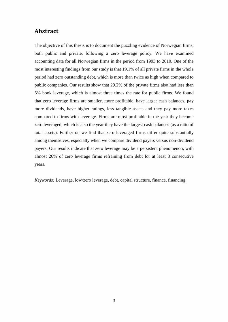
Abstract

The objective of this thesis is to document the puzzling evidence of Norwegian firms,

both public and private, following a zero leverage policy. We have examined

accounting data for all Norwegian firms in the period from 1993 to 2010. One of the

most interesting findings from our study is that 19.1% of all private firms in the whole

period had zero outstanding debt, which is more than twice as high when compared to

public companies. Our results show that 29.2% of the private firms also had less than

5% book leverage, which is almost three times the rate for public firms. We found

that zero leverage firms are smaller, more profitable, have larger cash balances, pay

more dividends, have higher ratings, less tangible assets and they pay more taxes

compared to firms with leverage. Firms are most profitable in the year they become

zero leveraged, which is also the year they have the largest cash balances (as a ratio of

total assets). Further on we find that zero leveraged firms differ quite substantially

among themselves, especially when we compare dividend payers versus non-dividend

payers. Our results indicate that zero leverage may be a persistent phenomenon, with

almost 26% of zero leverage firms refraining from debt for at least 8 consecutive

years.

Keywords: Leverage, low/zero leverage, debt, capital structure, finance, financing.

3

Preface

This thesis was written as a part of our master degrees at the Norwegian School of

Economics (NHH), and corresponds to one semester of full-time studies.

Our interest for the particular theme of the thesis started as a curiosity of why Apple

Inc. chose to have zero debt while all the capital structure theories we knew about at

the time would suggest a higher debt ratio for such a company. Our supervisor

showed us some recent articles on the theme, which started our fascination for the

zero leverage mystery.

Our work with this thesis has been both challenging and rewarding, not to mention a

huge learning experience. The choice of working together was an easy one to make,

as we have known each other for some time and are both interested in the same fields

within financial economics. We believe our collaboration, through discussions and

mutual feedback, has strengthened our work, and been especially beneficial when we

have met difficult challenges along the way.

We hope this thesis will contribute to the interesting field of corporate finance, and

that it will shed light on the zero leverage mystery with regard to Norwegian firms.

We would like to thank SNF (Institute for Research in Economics and Business

Administration) for providing us with the necessary data.

Last, but not least, we would to like express our sincere gratitude to our supervisor

Michal Kisser for support and valuable feedback throughout the process.

Bergen, June 14th 2013.

Fredrik Bruskeland Alexander C. C. Johansen

4

Contents

Abstract .......................................................................................................................... 3

Preface............................................................................................................................ 4

List of tables ................................................................................................................... 7

List of figures ................................................................................................................. 8

1 Introduction ............................................................................................................ 9

1.1 Problems to address ........................................................................................ 10

1.2 Limitations ...................................................................................................... 10

1.3 Structure .......................................................................................................... 11

2 Capital structure theory ...................................................................................... 12

2.1 Capital structure irrelevance: Modigliani-Miller ............................................ 12

2.1.1 Modigliani-Miller I .................................................................................. 12

2.1.2 Modigliani-Miller II ................................................................................. 13

2.2 The effect of the interest tax shield: Modigliani-Miller .................................. 14

2.3 Trade-off theory .............................................................................................. 16

2.3.1 Static Trade-off Theory............................................................................ 16

2.3.2 Dynamic Trade-off models ...................................................................... 18

2.4 Agency cost theories ....................................................................................... 19

2.5 Pecking order theory ....................................................................................... 20

2.6 Dynamic Financing and Investment Models .................................................. 20

2.7 Empirical evidence and research .................................................................... 22

2.7.1 The trade-off model ................................................................................. 22

2.7.2 Pecking order ........................................................................................... 23

2.7.3 The low/zero leverage mystery ................................................................ 24

3 Methodology ......................................................................................................... 27

3.1 T-Test .............................................................................................................. 27

5

3.2 Binary logistic regression ............................................................................... 27

3.3 The models ...................................................................................................... 29

4 The Data Source ................................................................................................... 30

5 Analysis ................................................................................................................. 32

5.1 Leverage definitions........................................................................................ 32

5.2 Fraction of zero/almost zero leveraged firms ................................................. 33

5.2.1 Public companies ..................................................................................... 33

5.2.2 Private consolidated groups ..................................................................... 35

5.2.3 Private companies .................................................................................... 36

5.3 Descriptive statistics ....................................................................................... 37

5.3.1 Private companies .................................................................................... 38

5.3.2 Private consolidated groups ..................................................................... 40

5.3.3 Public companies ..................................................................................... 41

5.3.4 Dividend and interest expense – Private companies ................................ 42

5.4 Industry ........................................................................................................... 46

5.5 Zero Leverage Event Study – Private companies ........................................... 48

5.6 ZL and AZL persistence ................................................................................. 51

5.7 Logistic Regression Analysis .......................................................................... 53

6 Concluding remarks ............................................................................................ 57

7 References ............................................................................................................. 59

Appendix 1: Definition of variables ............................................................................ 63

Appendix 2: Overview of industry classifications ....................................................... 64

Appendix 3: Industry breakdown – public firms and consolidated groups ................. 65

Appendix 4: Results from ZL event study ................................................................... 66

Appendix 5: Correlation matrices ................................................................................ 67

6

List of tables

Table 1: Fraction of ZL/AZLfirms – public companies .............................................. 34

Table 2: Fraction of ZL/AZLfirms – private consolidated groups .............................. 35

Table 3: Fraction of ZL/AZLfirms – private companies ............................................. 37

Table 4: Descriptive statistics ZL/AZLfirms – private companies .............................. 39

Table 5: Descriptive statistics ZL/AZLfirms – private consolidated groups ............... 41

Table 6: Descriptive statistics ZL/AZLfirms – public companies ............................... 42

Table 7: Dividend payers vs. non-dividend payers ...................................................... 44

Table 8: Industry breakdown – private firms ............................................................... 47

Table 9: ZL/AZL persitence ........................................................................................ 52

Table 10: Logit regression. Determinants of ZLpolicy ............................................... 54

7

List of figures

Figure 1: The WACC with and without corporate taxes ............................................. 15

Figure 2: Optimal leverage with taxes and bankruptcy costs ...................................... 17

Figure 3: Dividend and interest expense – private firms ............................................. 45

Figure 4: Zero leverage event study............................................................................. 49

8

1 Introduction

In 1958 Franco Modigliani and Merton H. Miller published a well known, and often

cited, article called “The Cost of Capital, Corporation Finance and the Theory of

Investment”. The model outlined in this article suggested that capital structure is

irrelevant for the value of a firm in perfect capital markets. However, when they

include corporate taxes they find that an increase in debt will increase the firm value

due to the fact that interest payments are tax deductible, and dividends are not.1 This

article formed the basis for modern thinking on capital structure and has been an

important inspiration for other famous capital structure theories such as the trade-off

theory and the pecking order theory. These theories have received different kinds of

criticism, but perhaps the most important being the observation that firms seem to be

too conservative in their use of debt. Graham (2000) finds for instance that the typical

firm could double its tax benefits by issuing more debt.

Although this low leverage puzzle is interesting, recent studies of capital structure

have shed light on another puzzling phenomenon, which we find even more

interesting. Strebulaev and Yang (2013) call this phenomenon “the zero-leverage

puzzle”, and the puzzle is that a high fraction of firms choose to have zero

outstanding debt. Such extreme debt conservatism cannot be explained by existing

capital structure theories, and a study of this puzzle is therefore important to get a

better understanding of financing decisions. Strebulaev and Yang (2013) find that

between 1962 and 2009, on average 10.2% of large public non-financial US firms had

zero outstanding debt, and 32% had zero or negative net debt. This is surprisingly

high. They also find that 61% of firms with zero outstanding debt show no propensity

to issue debt in the next year. Because the fraction of zero-leveraged firms is so high,

they argue that the low-leverage puzzle can be replaced by the zero-leveraged puzzle.

They back up this claim by showing that if you exclude all firms with a book leverage

of less than 5% the average book leverage increases from 25% to 32%. Dang (2012)

did a similar study on UK-firms and found that in the period between 1980 and 2007

the fraction of zero-levered firms was on average 12.18%.

1 see MM (1958) and MM (1963)

9

Strebulaev and Yang (2013) also argue that studying zero-leverage behaviour can be

advantageous from an empirical perspective, because the factors that lead firms to

become low-levered are more likely to be dominating for zero-leverage firms.

1.1 Problems to address In this thesis we focus on Norwegian companies and try to replicate parts of the study

in Strebulaev and Yang (2013) and Dang (2012). To our knowledge, such an analysis

has never been done on Norwegian companies before. In addition to studying public

companies, we have extended the study to also include private companies in order to

see whether there exists a difference between these two groups.

Throughout the thesis we will try to find out if there are significant differences in

characteristics between levered and zero-levered firms, and we will also try to find

economic mechanisms that drive companies to become zero-levered.

1.2 Limitations One of the most important differences between this thesis and similar studies on zero-

leverage firms is the use of proxies. Strebulaev and Yang (2013) construct a set of

proxies for each zero-leverage observation, which they find by identifying up to four

firms that have the same industry code and are the closest to the observed firm in size.

They have no restriction on leverage, meaning that the proxies may also be firms with

zero outstanding debt. They then compare characteristics between zero-levered firms

and their proxies. A big advantage by using such kind of proxies is that they can

conclude that differences in characteristics are not caused by differences in size or

industry. Dang’s (2012) study is similar; like Strebulaev and Yang (2013) he creates

proxy firms, but at the same time he also compares zero-leverage firms with levered

firms. Constructing these kinds of proxies is a complex process and beyond our

knowledge. We have therefore chosen to only compare zero-/low- leveraged firms

with levered firms. As a consequence we cannot make the same conclusions as

Strebulaev and Yang (2013) and Dang (2012), but we still believe a comparison

between levered and zero-levered firms can reveal important factors that may lead

firms to adopt a zero-leverage policy.

10

Another limitation in our thesis is that our dataset does not provide us with market

information such as market values and share repurchases. Both Strebulaev and Yang

(2013) and Dang (2012) use the market-to-book ratio to reflect a firm’s growth

opportunities. Several theories such as Myers (1977) and DeAngelo et al. (2011) say

that firms with high growth opportunities have less incentive to take on debt. This is

therefore an interesting measure when comparing levered and unlevered firms. Share

repurchases is an important measure to get an overview of a firm’s total payout.

Information about a firm’s total payout is important to see whether zero-leveraged

firms retain a higher fraction of their earnings to be able to fund future investments.

Our dataset only provides us with dividends and we are therefore forced to use this as

an approximation of total payout.

Finally we see it as a small limitation that there are few publicly listed companies in

Norway. While Strebulaev and Yang (2013) have on average 4,129 firm observations

in each year between 1987 and 2009, we have an average of 117 in our period. This

makes it more difficult to find significant differences between leveraged and zero-

leveraged public firms. However, as we will show, the most interesting part of our

thesis is the study on private firms, and here we have a yearly average of 19,187 firm

observations.

1.3 Structure The thesis is structured as follows: Section 2 provides a presentation of some of the

most important existing theories on capital structure. This section is meant to give an

insight into why such a large fraction of firms choose to have zero outstanding debt

can be called a mystery. Section 3 describes the methodology we have used in parts of

our analysis, and section 4 explains the data set we have used. In section 5 we present

the results of our analysis and section 6 concludes. Appendices are found at the end of

the thesis.

11

2 Capital structure theory

The relative proportions of a firm’s outstanding securities constitute its capital

structure. When a firm needs new funds to undertake its investments it has to decide

which type of security to issue to potential investors, the most common choices of

financing being debt and equity. Even without the need for new capital a firm might

still decide to acquire financing and use the raised funds to either repay debt or

repurchase shares. In this section we present existing capital structure theory, research

and empirical evidence to outline some of the most important considerations and

choices firms have to make when deciding a capital structure, e.g. how such choices

affect the valuation of the firm and its profitability. This section will then serve as a

theoretical background in understanding why the decision to have zero leverage is in

fact a mystery.

2.1 Capital structure irrelevance: Modigliani-Miller Modigliani and Miller (from now: MM) (1958) argued that capital structure was

irrelevant and would not affect a firm’s value under a set of conditions referred to as

perfect capital markets: 1) There are no taxes, transaction costs, issuance costs or

arbitrage opportunities. 2) Commodities which can be regarded as perfect substitutes

must sell at the same price in equilibrium. 3) The financing decisions of a firm do not

change the underlying cash flows of its investments, nor do they reveal new

information about them.

Under these conditions MM (1958) set forth a couple of propositions regarding firm

value and the cost of capital.

2.1.1 Modigliani-Miller I

MM Proposition I: “The market value of any firm is independent of its capital

structure and is given by capitalizing its expected return at the rate pk appropriate to

its class.” (Modigliani and Miller, 1958 p. 8)

MM (1958) assumed that firms could be divided into equivalent return classes,

denoted by k. The expected rate of return for each class is then denoted by pk. Further

12

on, MM (1958) argued that the total cash flow generated by a firm’s assets should

equal the total cash flow paid out to the security holders of the firm. By the law of one

price, the firm’s outstanding securities and its assets must have the same market

value. As the issuance of any type of security in a perfect capital market does not

change the underlying cash flows of a firm’s assets, the capital structure of the firm is

irrelevant.

Should investors, for some reason, prefer a different capital structure than the firm,

MM (1958) showed that they could create their own capital structure by borrowing or

lending money on their own. This is called homemade leverage. Under the condition

that the investors can borrow and lend money at the same interest rates as the firm,

homemade leverage will act as a perfect substitute for any capital structure of the

firm.

2.1.2 Modigliani-Miller II

MM Proposition II: “The expected yield of a share of stock is equal to the

appropriate capitalization rate pk for a pure equity stream in the class, plus a

premium related to financial risk equal to the debt-equity ratio times the spread

between pk and r.” (Modigliani and Miller, 1958 p. 11)

MM (1958) proposition II states that an all equity firm has an expected return, ij,

equal to pk, while a leveraged firm has an expected return equal to pk, plus pk minus

the cost of debt, r, times that firm’s debt to equity ratio, Dj/Sj. As the proposition

holds for realized returns it also holds for expected return.

𝑖𝑗 = 𝑝𝑘 + (𝑝𝑘 − 𝑟)𝐷𝑗/𝑆𝑗

(1)

With proposition I MM (1958) showed that the value of a firm does not depend upon

its choice of capital structure, rather it comes from the underlying cash flows of the

firm’s assets and the firm’s cost of capital. The cost of debt and the cost of equity

often differ quite a bit, the cost of debt usually being lowest. One might therefore

think that increasing a firm’s leverage ratio would lower the cost of capital and

increase the value of the firm. MM (1958) proved that this is not the case, as adding

13

more debt (Dj) will increase the risk and therefore the cost the firm’s equity (ij). They

showed that the savings gained from the lower cost of debt will be perfectly offset by

the increased cost of equity, and subsequently the firm’s weighted average cost of

capital (WACC) will stay unchanged.

2.2 The effect of the interest tax shield: Modigliani-Miller MM’s propositions (I and II) provide useful insights into the world of corporate

finance, however there is no such thing as a perfect capital market. Two market

imperfections that are essential for firms are corporate taxes and the tax deductibility

of interest payments. Combined, these two imperfections play a large role in

determining the capital structure of firms.

Firms have to pay taxes on their earnings, but only after interest payments are

deducted. This interest tax deduction will lower the amount of taxes the firm has to

pay, assuming the firm has positive earnings, and thus there exists an incentive to use

debt. Although interest payments will reduce the amount of cash available to the

equity holders of the firm, the total amount of cash the firm can pay out to all its

investors, the free cash flow to the firm (FCFF), will be higher due to the interest tax

shield. A consequence of the firm’s ability to pay out more cash to its investors is that

it will have increased its value. This increase in value exactly matches the gain arising

from the interest tax shield, which can be calculated each year as follows:

𝐼𝑛𝑡𝑒𝑟𝑒𝑠𝑡 𝑡𝑎𝑥 𝑠ℎ𝑖𝑒𝑙𝑑 = 𝑐𝑜𝑟𝑝𝑜𝑟𝑎𝑡𝑒 𝑡𝑎𝑥 𝑟𝑎𝑡𝑒 ∗ 𝑖𝑛𝑡𝑒𝑟𝑒𝑠𝑡 𝑝𝑎𝑦𝑚𝑒𝑛𝑡𝑠 (2)

The cash flow from a firm with leverage is equal to the cash flow from a firm without

leverage plus the interest tax shield. By the law of one price the same must be true for

the present values of these cash flows. In the presence of taxes MM (1958, 1963)

showed that the value of a levered firm, VL, would exceed the value of the firm

without leverage, VU, due to the present value of the tax savings from debt, PV(TS).

𝑉𝐿 = 𝑉𝑈 + 𝑃𝑉(𝑇𝑆) (3)

14

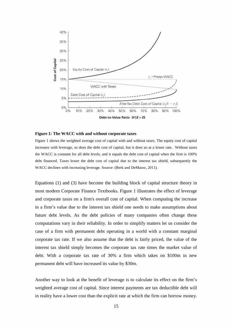
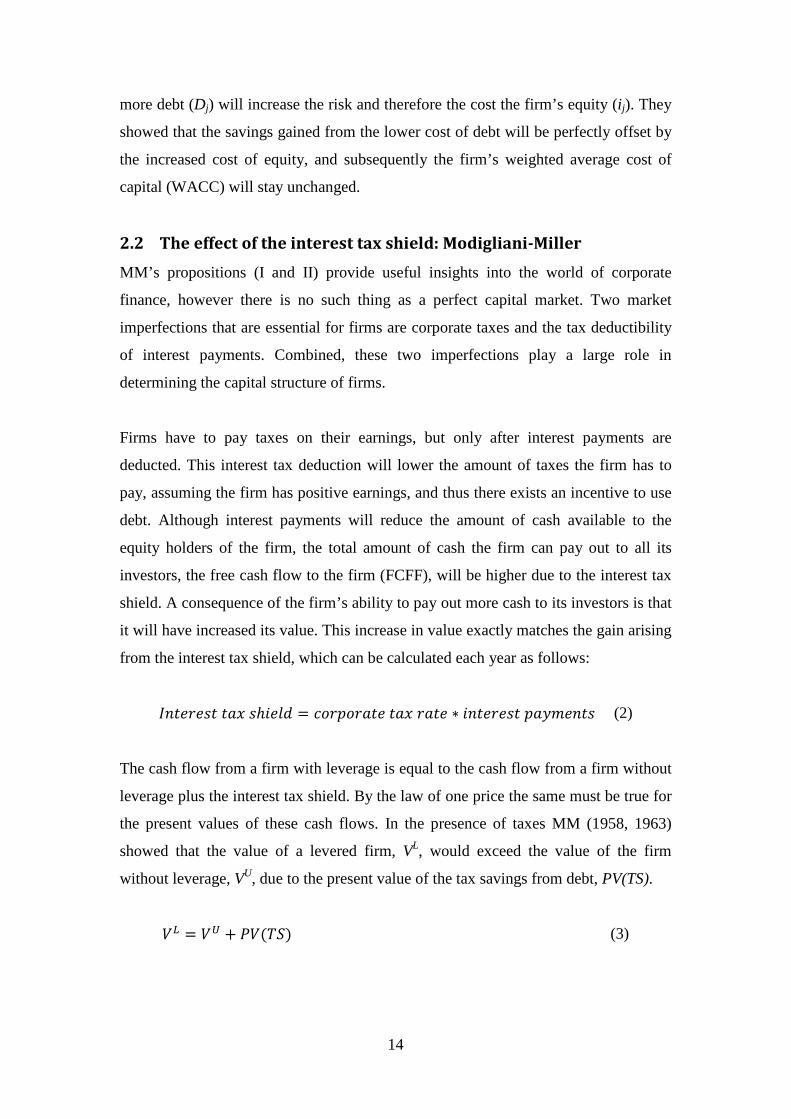
Figure 1: The WACC with and without corporate taxes Figure 1 shows the weighted average cost of capital with and without taxes. The equity cost of capital

increases with leverage, so does the debt cost of capital, but it does so at a lower rate. Without taxes

the WACC is constant for all debt levels, and it equals the debt cost of capital when the firm is 100%

debt financed. Taxes lower the debt cost of capital due to the interest tax shield, subsequently the

WACC declines with increasing leverage. Source: (Berk and DeMarzo, 2011).

Equations (1) and (3) have become the building block of capital structure theory in

most modern Corporate Finance Textbooks. Figure 1 illustrates the effect of leverage

and corporate taxes on a firm's overall cost of capital. When computing the increase

in a firm’s value due to the interest tax shield one needs to make assumptions about

future debt levels. As the debt policies of many companies often change these

computations vary in their reliability. In order to simplify matters let us consider the

case of a firm with permanent debt operating in a world with a constant marginal

corporate tax rate. If we also assume that the debt is fairly priced, the value of the

interest tax shield simply becomes the corporate tax rate times the market value of

debt. With a corporate tax rate of 30% a firm which takes on $100m in new

permanent debt will have increased its value by $30m.

Another way to look at the benefit of leverage is to calculate its effect on the firm’s

weighted average cost of capital. Since interest payments are tax deductible debt will

in reality have a lower cost than the explicit rate at which the firm can borrow money.

15

This insight implies that an increase in the debt ratio of a firm will lower a firm’s

WACC. Consequently future cash flows will have a higher present value, which will

match the present value of the interest tax shield.

2.3 Trade-off theory As shown in the section above, Modigliani and Miller’s (1963) model created a

benefit for debt when corporate income tax was included. Since the model assumes

that there are no costs associated with a change in leverage it suggests extreme debt

levels. Such extreme debt levels are not observed in the real world and the model

therefore needs to include some sort of offsetting cost of debt to be more realistic.

Several different authors have presented theories that include different forms of such

costs. The term trade-off theory has been used to describe these theories. They all

have in common that the costs and benefits of alternative financing methods are

evaluated by a decision maker who runs the firm. The optimal solution is found where

the marginal costs equal the marginal benefits.

In this paper we divide the trade-off theories into two main categories; Static- and

Dynamic trade-off theory. The former category consists of single period trade-off

theories that do not recognize the role of time and assume that a firm’s leverage is

determined by a trade-off between tax benefits and costs of bankruptcy. Dynamic

trade-off theory also considers such a trade-off. However, at the same time, it

recognises adjustment costs associated with refinancing and fluctuations in asset

values over time.

2.3.1 Static Trade-off Theory

Kraus and Litzenberger (1973) provide a classic trade-off model where corporate

taxes and bankruptcy costs are put into a single-period valuation model in a complete

capital market. Their intuition is that for a certain level of leverage, the bankruptcy

costs will equal the advantage of decreased taxes, and the value of the company is

therefore maximised at this level. A simple mathematical explanation of their model

is presented in equation (4).

𝑉𝐿 = 𝑉𝑈 + 𝑃𝑉(𝑇𝑆) − 𝑃𝑉(𝐵𝐶) (4)

16

Figure 2: Optimal leverage with taxes and bankruptcy costs Figure 2 shows that for a certain level of leverage (D*) for each firm the gains from increasing debt are

completely offset by the increase in bankruptcy costs. This is the level of leverage that maximises the

company value. It also shows that the company with high bankruptcy costs (distress costs) has a lower

optimal level of leverage than the company with low bankruptcy costs. Source: (Berk and DeMarzo,

2011).

Equation (4) states that the total value of a leveraged company (VL) is given by the

value of the company if it has no leverage (VU) plus the present value of the interest

tax shield (PV(TS)) minus the present value of bankruptcy costs (PV(BC)). An

increase in leverage is associated with an increase in the tax shield, which increases

the firm value, but such an increase also leads to an increase in bankruptcy costs,

which again lowers the firm value. The firm value is maximised when the marginal

benefits of the tax shield equals the marginal cost of bankruptcy.

To calculate a precise value of the bankruptcy costs is complicated and this has been

done in different ways by different authors. Weiss (1990) classifies the bankruptcy

costs as either direct or indirect bankruptcy costs, where direct costs are related to the

costs of an actual bankruptcy, while indirect costs are costs that arise before a possible

bankruptcy. Examples of the latter are loss of competiveness, poor credit terms or

17

broken contracts, while direct bankruptcy costs can be legal- and audit expenses or

cost of liquidating assets (because they are often sold at fire sale prices).

Since companies face different tax rates and levels of bankruptcy costs, this theory

implies that each company has a distinctive optimal level of leverage. Figure 2 shows

different optimal levels of leverage for three firms with different levels of bankruptcy

costs. Logically, a firm with high bankruptcy costs has a lower optimal level of

leverage than a firm with low bankruptcy costs.

2.3.2 Dynamic Trade-off models

In contrast to static trade-off models, dynamic models recognise the role of time.

Fischer, Heinkel and Zechner (1989) were the first to develop a dynamic trade-off

model that recognises that a firm’s optimal structural choices are dependent on

transaction costs and the fluctuations in asset values over time. In their model firms

still consider a trade-off between tax benefits and bankruptcy. However, because there

are transaction costs associated with a recapitalisation, firms will refinance only

occasionally. In other words, a firm will not refinance until the benefit of the

refinancing outweighs the cost. This implies that there is not one distinctive optimal

leverage ratio, but an optimal range. As long as a firm’s leverage stays within this

range, it has no incentive to recapitalise. The size of this range is dependent on the

variables included in the model. They argue that a decrease in the corporate tax rate or

bankruptcy costs will widen the range. The same counts for an increase in the

variance of asset values.

Strebulaev (2007) provides a similar model as the one in Fischer, Heinkel and

Zechner (1989). An important aspect with this model is that it highlights the

difficulties in interpreting the relationship between leverage and profitability; an

aspect in which empirical studies have found the trade-off model to fail. As

previously shown, an increase in a firm’s profitability will in the trade-off model

reduce the expected bankruptcy costs and therefore gives the firm the opportunity to

increase its tax benefits by increasing leverage. The model therefore states that the

leverage-profitability relationship should be positive. However, empirical studies such

as Myers (1993) have found this relation to be negative. This observed negative

18

relation has been perhaps the most important criticism raised against the trade-off

model.

The model in Strebulaev (2007) shows that economy dynamics can explain the

negative relationship. His model suggests that expected profitability and leverage is

positively correlated at a refinance point. This is consistent with the traditional trade-

off models, but the model also suggests that in a dynamic economy the relationship is

negative. The intuition behind this is that when firms do not refinance, an increase in

profitability will increase the future profitability and therefore also the value of the

firms. This results in a lower market and book leverage, ceteris paribus. In the

simulations of the model, there are firms that refinance in any period, but the firms

that do not do so dominate. Consequently the model shows a negative relationship

between profitability and leverage.

2.4 Agency cost theories Agency cost theory defines corporate managers as agents for shareholders and

analyses the conflicting interest between them. This conflict exists because

shareholders want the company to be run in a way that maximises their value, but

management has incentives to maximise their personal power and wealth. This may

not be in the best interests of the shareholders. Since they cannot control all the

decisions made by the managers there exists informational asymmetries between

them, and this can lead to agency costs.

Jensen (1986) points out that the conflicting interest between the shareholders and

management are particularly severe when the company has a substantial amount of

free cash flow. This is mainly because there is a greater possibility that the

management will, for personal reasons, invest some of this free cash flow in projects

that generate returns below the company’s cost of capital. The idea behind the agency

cost theory is that shareholders can constrain management by increasing the company

leverage, and thereby decrease the amount of free cash flow. However, under the

section “The Role of Debt in Motivating Organizational Efficiency” Jensen (1986)

also points out that an increase in leverage will not always have a positive control

effect. For instance fast growing companies with many high profitable investment

19

opportunities, but with a low amount of free cash flow, will commonly need to turn to

the financial markets to obtain capital. For each capital raise, the markets have the

option to evaluate the proposed projects and the company management. As long as

this option is used in an efficient manner the gains of increasing leverage for control

purposes is petite.

2.5 Pecking order theory Pecking order theory suggests that there exists asymmetric information between the

managers of a firm and the stockholders, and that both parties are aware of this.

Myers and Majulf (1984) argue that as long as this asymmetric information exists,

managers will prefer internal- to external financing. The logic being that this

condition will lead to an under-pricing of the firm’s equity because managers will

always have incentives to issue new equity when the stock is overpriced. However, as

long as external investors are aware of this, an equity issue sends a strong pessimistic

signal to the market. The managers will also try to avoid an equity issue if the stock is

under-priced, and if this happens at the same time as the firm has an investment

opportunity managers might disregard the investment even if it has a positive NPV.

This is called “the underinvestment problem”.

Myers and Majulf (1984) go on by defining a rating of the different financing options

where the idea is that managers will chose the best-rated option first. More precise;

the managers will choose internal financing (financial slack) first, then debt. Hybrid

securities (as convertible bonds) are the third option, and finally issue of new equity.

The pecking order theory therefore violates the other theories presented earlier as

managers are not trying to achieve a certain level of leverage, but rather issue debt

and equity when financing is required. In other words, according to this theory, if a

firm has enough cash to undertake all of its possible investments (with a positive

NPV) the managers of the firm will not issue any debt or new equity.

2.6 Dynamic Financing and Investment Models Although traditional capital structure theory suggests that the optimal debt ratio is the

one that maximizes the value of a firm, evidence has shown that firms typically hold

20

debt levels below this optimal point. Dynamic financing and investment models

(starting with Hennessy and Whited, 2005) combine elements of both trade-off and

pecking order theories and generally produce more "realistic" leverage ratios.

According to DeAngelo, DeAngelo and Whited (2011) optimal leverage targets

include the option to issue transitory debt, thus allowing firms to handle (unexpected)

investment needs, referred to as investment shocks. To fund such shocks firms often,

deliberately – but temporarily – deviate from their leverage targets by issuing

transitory debt.

Transitory debt refers to the difference between actual and target debt levels, and is

not necessarily all of a firm’s short term debt; it is simply debt that managers intend to

pay off in the short to intermediate term to free up debt capacity. Rather than the

duration of the debt, it is managerial intent that defines whether or not the debt is

transitory.

In DeAngelo et al.’s (2011) dynamic capital structure model the target capital

structure of firms and their use of transitory debt is directly related to the nature of

their investment opportunities because “(i) borrowing is a cost-efficient means of

raising capital when a given shock to investment opportunities dictates a funding

need, and (ii) the option to issue debt is a scarce resource whose optimal

intertemporal utilization depends on both current and prospective shocks.”

(DeAngelo et al. 2011, p. 1). The option to issue debt is valuable since the model, in

contrast to extant trade-off models, assumes that investment decisions are

endogenous, and that all forms of financing are costly. Other dynamic capital

structure studies also state the importance of endogenous investment, see for example

Tserlukevich (2008), Morreles and Schürnoff (2010), and Sundaresan and Wang

(2006), who study the leverage impact of real options. The assumption of endogenous

investment policy is critical to the model, with variation in investment opportunity

attributes being the main driver behind the models predictions.

The takeaway here is that debt capacity is a finite – and limited – resource, while at

the same time being the cheapest form of external financing for a firm (where

cheapest is defined as involving the lowest financing costs). It therefore stands to

21

reason that firms would prefer to issue debt to fund investment shocks. As a result

they would have to keep their debt levels below target, and retain the option to issue

debt.

If a firm issues debt today it also must include the opportunity cost of its consequent

future inability to borrow when calculating the relevant leverage-related cost. This

opportunity cost implies that target capital structures are even more conservative. A

firm’s long run target debt level, when viewed ex ante, is then the level that optimally

balances the tax shield from debt, distress costs of debt and the opportunity cost of

using debt capacity now.

Further on, the model shows that the amount of outstanding debt of firms is inversely

related to the volatility of unexpected investment shocks, meaning that firms who

experience unpredicted investment needs tend to have less debt. While, on the other

hand, firms that have more predictable future investment needs, or lower volatility of

investment shocks, tend to have more debt outstanding. The conclusion being that the

higher the degree of investment shock volatility the more valuable it is for firms to

preserve debt capacity. On average, the benefit of preserving debt capacity outweighs

the negative impact of the loss of the interest tax shield due to lower debt ratios.

DeAngelo et al. (2011) also show that firms who face high investment shock volatility

rely more on (tax disadvantaged) cash balances to fund investment, as unused debt

capacity might not suffice, thus reducing their net debt even further. In such cases

maintaining cash balances is the preferable option compared to costlier equity

financing.

2.7 Empirical evidence and research In this section we will outline literature that reviews how the traditional capital

structure theories hold up empirically. We will also give an insight on research into

the zero-leverage mystery.

2.7.1 The trade-off model

As previously mentioned, the static trade-off model, building on the results of

Modigliani and Miller (1958), suggests that firms choose their capital structure to

22

balance the costs and benefits of debt financing. In their review of empirical capital

structure studies Graham and Leary (2011) find that “...several cross-sectional

patterns in leverage are broadly consistent with this view.” (Graham and Leary, 2011

p. 9).

According to the trade-off model, within-firm deviations from leverage targets are

costly and should be corrected. Jalilvand and Harris (1984) present evidence of

within-firm mean-reversion of leverage ratios, which is consistent with the trade-off

view. However, Graham and Leary (2011) find important shortcomings in empirical

studies of the trade-off model. According to the model more profitable firms, ceteris

paribus, should value the tax-shield benefits of debt higher. Nonetheless, many

authors point out that there is a negative relation between leverage and profitability,

which goes against the view of the trade-off model.

Further, Graham and Leary (2011) point out that many firms have low leverage

despite facing low distress risk and heavy tax burdens. Other studies, e.g. Fama and

French (2002) and Iliev and Welch (2010), suggest that the observed speed of

adjustment towards leverage target is too slow to be consistent with the static trade-

off model. According to Myers (1993) the aforementioned model may be a weak

guide to average firm behaviour, and he states that it doesn’t help much in

understanding the decisions of any given firm.

2.7.2 Pecking order

The pecking order theory of Myers and Majluf (1984) is a traditional alternative to the

trade-off theories. Like the trade-off model it discusses the costs and benefits of

capital structure decisions (all capital structure theory does), but the theories differ

with regards to which market frictions are most important.

Graham and Leary (2011) state that the promise of the pecking order theory lies

within its consistency with two main empirical findings: “(i) there is a significant

negative market reaction to the announcement of seasoned equity issues; and (ii) in

aggregate, firms fund the majority of investments with retained earnings while

aggregate net equity issues often are small or even negative.” (Graham and Leary

2011, p. 11).

23

In support of the pecking order theory, studies by Shyam-Sunders and Myers (1999)

and Helwege and Liang (1996) have shown a strong correlation between the

retirement/issuance of debt and a firm’s need for external financing. A study by Frank

and Goyal (2003) has provided different results, they show that smaller and younger

firms prefer equity issues when they are in need external financing. Fama and French

(2005) report similar results, they find that small and high growth firms prefer equity

issues over debt.

In support of the pecking order Lemmon and Zender (2010) point out that small firms

may be constrained by limited debt capacity, and therefore the findings of Fama and

French (2005) may not be inconsistent with the traditional theory.

A study by Leary and Roberts (2010) finds that the pecking order struggles to predict

capital structure decisions, over a range of subsamples. While Myers (2001) finds,

overall, that the pecking order might be a useful conditional theory. However it still

leaves many financing decisions unexplained.

2.7.3 The low/zero leverage mystery

Although some of the models we have mentioned might explain why some firms have

low leverage, or at least lower leverage than "target", none of them are able to explain

why such a large portion of firms take their capital structure decisions to the extreme

and choose almost zero, or zero, leverage.

In a recent empirical study, Strebulaev and Yang (2013) document the puzzling

evidence that a large fraction of U.S. publicly traded firms follow a zero leverage

policy. They find that, on average, over the period from 1962 to 2009 10.2% of these

firms have zero debt, and almost 22% have less than a 5% book leverage ratio.

Further on they find that as firms become less and less leveraged they effectively

replace interest costs with dividend payments, thus keeping the total payout of firms

relatively stable across the leverage spectrum.

A decision by a firm to have zero leverage is also not a short term deviation from

target leverage. The evidence suggests that it is a persistent phenomenon. 61% of

24

firms with no debt, in any given year, show no inclination of acquiring debt the

following year, and as much as 30% of zero leverage firms follow such a policy for at

least 5 consecutive years.

To understand the nature of zero leverage behaviour better Strebulaev and Yang

(2013) construct a set of proxy firms, chosen by industry and size, for each zero

leverage firm-year observation. These proxy firms then serve as control observations.

The evidence shows that ZL firms and their proxies differ significantly along a

number of dimensions: on average ZL firms are more profitable, pay more dividends,

pay more income taxes, have less tangible assets, have higher cash balances, and they

are smaller.

They also find that ZL firms give up a substantial amount of tax benefits of debt, on

average they leave 7.6% of their market values on the table by choosing not to lever

up. This only reinforces the mystery of why some firms chose such an extreme debt

policy.

According to their study, neither industry nor size can explain this puzzling

phenomenon. However, they find that family owned firms and firms with higher CEO

ownership and longer CEO tenure are more likely to adopt a ZL policy. Their results

suggest “that managerial and governance characteristics are related to the zero-

leverage phenomenon in an important way.” (Strebulaev and Yang, 2013, pp 2)

In a similar study, concentrating on UK firms, Dang (2012) finds comparable results.

Over a sample period between 1980 and 2007 he finds that 12.18% of publicly listed,

non-financial, firms in the UK have zero outstanding debt, which is even higher than

Strebulaev and Yang (2013). In the period between 2000 and 2007 almost 20% of

such firms followed a zero leverage policy.

He finds that ZL firms are smaller and younger, that they have less tangible assets,

pay higher dividends and have larger cash holdings, compared to their proxy firms.

Also firms with higher growth opportunities are more likely to become zero

leveraged. In contrast to Strebulaev and Yang (2013) he finds that ZL firms are less

profitable then their proxies. The evidence also shows that ZL firms with less cash

25

holdings and growth opportunities, but more capital expenditures, are more likely to

become leveraged.

Even though ZL firms differ from their proxy firms and from leveraged firms among

many dimensions, both studies, Strebulaev and Yang (2013) and Dang (2012), agree

that zero leverage behaviour remains a mystery. A model which can fully explain this

phenomenon remains to be found.

26

3 Methodology

This section will be used to discuss the methodology used in parts of the upcoming

analysis. Since there has been little empirical research earlier on the theme of this

thesis a large part of the analysis will be descriptive data, which has a fairly

straightforward methodology. This type of analysis will not be discussed in this

section.

3.1 T-Test In one part of the analysis we present a comparison between zero leveraged- and

leveraged firms across different dimensions. To get a better understanding of the

difference between the two samples, for each reported variable, we first perform an F-

test to check for either equal or unequal variances. Then we perform an independent

two sample pairwise T-test, for either equal or unequal variances, both samples with

unequal sample sizes. The T-test shows whether there is a significant difference

between the average values of the two categories (i.e. zero leveraged and leveraged)

for the variable in interest.

3.2 Binary logistic regression We are interested in exploring the properties of zero-leveraged (ZL) firms and we will

therefore run a regression with ZL as the dependent variable. Since ZL is a binary

variable (i.e. can only take on two possible values) a standard linear regression model

will in this case have certain shortcomings. The two most important being that the

coefficient’s marginal partial effects are constant and that the predicted probabilities

can take on values that are not within the range of zero to one. Instead, we will

therefore use a binary response model (hereafter referred to as “logit-model”), which

is shown in equation (5). (Wooldridge, 2009)

𝑃(𝑦 = 1|𝑥) = 𝐺(𝛽0 + 𝛽1𝑥1 + ⋯+ 𝛽𝑘𝑥𝑘) 𝑤ℎ𝑒𝑟𝑒

𝐺(∙) = 𝐺(𝑧) =𝑒𝑧

1 + 𝑒𝑧

(5)

27

This model estimates the probability (P) of the dependent binary variable (y) to have

an outcome of 1, given the explanatory variables (x1-xk). The explanatory variables

have coefficients (β1 – βk) and G(z) is a function which ensures that the predicted

probabilities are always between zero and one for all real numbers z.

Aldrich and Nelson (1984) discuss two important assumptions, in addition to what is

already mentioned, that need to be fulfilled for the logit-regression to be valid. The

first one being that the observations of the explanatory variables need to be

independent from each other. Since we are using panel data, observations for each

firm in different years are highly correlated. This violates the mentioned assumption.

To adjust for this we run the regression with standard errors clustered at the firm

level. The second assumption is that there cannot be a strong linear connection

between two or more of the explanatory variables. We have therefore carefully chosen

explanatory variables that are not expected to have this kind of relationship. The

pairwise correlations between the selected variables are presented in Appendix 5. The

level of correlation is similar to other studies on the same theme, as for instance Dang

(2011).

A weakness with the logit-model is that the coefficients are not as easily interpreted

as in a standard linear regression. Whereas the coefficients in a linear regression will

show how much a one unit increase in the independent variable will change the

outcome of the dependent variable, the interpretation of coefficients in the logit-

model are a little more defuse. Since the function G is non-linear, the marginal partial

effects of the coefficients are not constant. Consequently, if the value of one

independent variable is changed, or another one is included, the coefficients and the

marginal partial effects of all the other variables will change as well.

Wooldridge (2009) suggests mainly two different methods for presenting the

independent variables’ effect on the dependent variable; the partial effect of the

average (PEA) and average partial effect (APE).

The PEA method replaces the independent variables with their average and then

reports the marginal effects of the average observation in the sample. Unfortunately,

this method does not work well if some of the dependent variables included in the

28

regression are discrete- or dummy variables. If for instance a dummy variable

recognises whether a company is listed on a public exchange and 35% of the

companies in the sample are listed it would not make any sense to use a value of .35

for the average company, as this is an impossible value to obtain.

To get around this problem it is possible to use the APE method instead. In this

method a coefficient represents the average marginal effect for all the values of the

corresponding explanatory variable in the sample. We will use this method when we

present our results in the coming analysis.

3.3 The models Since the coefficients for each explanatory variable of the binary logistic regression

are dependent on the level of the other explanatory variables included in the model we

run two different regressions, both with standard errors clustered at firm level. The

models are shown in equation (6) and (7).

𝐿𝑜𝑔𝑖𝑡 (𝑍𝐿) = 𝛼0 + 𝛼1𝑆𝑖𝑧𝑒 + 𝛼2𝑃𝑟𝑜𝑓𝑖𝑡𝑎𝑏𝑖𝑙𝑖𝑡𝑦 + 𝛼3𝐶𝑎𝑠ℎ +

𝛼4𝐴𝑔𝑒 + 𝛼5𝑇𝑎𝑛𝑔𝑖𝑏𝑖𝑙𝑖𝑡𝑦 + 𝛼6𝐼𝑛𝑖𝑡𝑖𝑎𝑙 𝑍𝐿 + 𝜀

(6)

𝐿𝑜𝑔𝑖𝑡 (𝑍𝐿) = 𝛽0 + 𝛽1𝑆𝑖𝑧𝑒 + 𝛽2𝑃𝑟𝑜𝑓𝑖𝑡𝑎𝑏𝑖𝑙𝑖𝑡𝑦 + 𝛽3𝐶𝑎𝑠ℎ +

𝛽4𝐴𝑔𝑒 + 𝛽5𝑇𝑎𝑛𝑔𝑖𝑏𝑖𝑙𝑖𝑡𝑦 + 𝛽6𝐼𝑛𝑖𝑡𝑖𝑎𝑙 𝑍𝐿 + 𝛽7𝑅&𝐷 +

𝛽8𝐶𝐸𝑂 𝑐𝑜𝑚𝑝 𝑎𝑏𝑠 + 𝛽9𝐼𝑛𝑑.𝐹𝑟𝑎𝑐 𝑍𝐿 + 𝜀

(7)

All the variables used in the two models are explained in Appendix 1.

29

4 The Data Source

We use accounting data for all Norwegian companies, both public and private, for the

years 1993 – 2010. The data set is divided into single company accounts and

consolidated group accounts for all years. The data set is made available by SNF

(Institute for Research in Economics and Business Administration) and NHH

(Norwegian School of Economics) through Aksel Mjøs and Karoline Øksnes.

All Norwegian companies owning subsidiaries, with ownership being above 50%,

have to file both company accounts and consolidated accounts. This results in

partially overlapping data sets. We merged the data sets and excluded single company

filings for parent companies, using only their consolidated accounts. We have also

excluded subsidiaries, as we assume that any major decision regarding debt and

capital structure is made by the parent company. The indication of subsidiary status is

only given for the years 2005 – 2010, and thus these years will be most accurate since

subsidiary companies will be included in the years before 2005. We have divided the

total sample into three categories: 1) private firms (including private consolidated

groups), 2) private consolidated groups and 3) public firms (listed on the Oslo stock

exchange).

In line with most capital structure research, this paper focuses on the debt structure of

mostly non-financial private and public companies. We have therefore excluded the

following industries, which are mainly financial companies, according to the

classification of NACE: 65 Financial intermediation, except insurance and pension

funding; 66 Insurance and pension funding, except compulsory social security; 75

Public administration and defence & compulsory social security; 91 Activities of

business, employers and professional organizations; 95 Activities of households as

employers of domestic staff. After this exclusion we are still left with a group of some

financial firms; even so, we believe we have excluded the most problematic, when

viewed in the light of capital structure research.

The data source includes all Norwegian companies, including sole proprietorships and

single person holding companies. We believe that many of these small firms may not

30

be representative for the data sample as a whole as their borrowing capacity is tied to

the personal wealth of the entrepreneur. We therefore exclude all observations (firm-

years) with either total revenues or total assets below NOK 5 million. Any firm-years

with missing values for total revenue or total assets have also been excluded, as we

will be using these variables in most of our study. Since we are only interested in

domestic Norwegian firms we have also excluded any non-Norwegian firms.

We are then left with a data set with varying degrees of firm-year observations for

each of our three categories: 1) private firms – 345,363 observations, 2) private

consolidated groups – 63,124 observations and 3) public firms – 2,112 observations.

31

5 Analysis

In this section we will report the results of our analyses. Many of the following

subsections are similar to Strebulaev and Yang (2013), i.e. the reporting of fractions

of various categories of low-leveraged firms, descriptive statistics, persistence studies

and logit regressions. Nonetheless our analyses still differ in many regards, for

instance we examine exclusively Norwegian firms. Whereas Strebulaev and Yang

(2013) only analyse publicly listed firms, we analyse both public and private firms.

We have also performed an event study focusing on the evolution of firms in the years

prior and posterior to the year in which they become zero leveraged.

5.1 Leverage definitions As previously explained, our dataset has been divided into three sub-categories;

public companies, private companies and private consolidated groups. For all three

categories we report the fraction of zero leveraged (ZL) firms. In line with Strebulaev

and Yang (2013), we have classified firms with zero or low leverage into four partly

overlapping categories. A firm is defined as a ZL firm in any given year if its amount

of interest bearing debt equals zero in that year.

As Strebulaev and Yang (2013), we compute the fraction of firms with zero long-term

debt for the sake of comparison. A firm is defined as a ZLTD firm in a given year if

that firm has zero long term debt outstanding. A difference in the fraction of ZL and

ZLTD will then indicate that some ZLTD firms carry some form of short-term debt.

The fraction of firms with zero long term debt will then almost always be higher than

that of zero leveraged firms.

If a firm in any given year has a book leverage of less than five percent it is classified

as an almost zero leverage (AZL) firm. Strebulaev and Yang (2013) point out several

reasons for why it might be interesting to look at AZL firms as well, the main reason

being that the existing theoretical models on capital structure suggest leverage ratios

that are well above zero:

“From a theoretical standpoint, a number of models (e.g., Fisher, Heinkel, and

Zechner (1989), Leland (1994), Leland and Toft (1996), Leland (1998), Goldstein, Ju,

32

and Leland (2001), Ju, Parrino, Poteshman, and Weisbach (2005)) produce leverage

ratios that are well above zero. Cross-sectional dynamics modelled by Strebulaev

(2007) may produce firms that are almost zero-leverage but in his benchmark case

their fraction is very low. Practically, the finance nature of various liabilities

assigned by accounting conventions to debt is ambiguous (for example, advances to

finance construction or instalment obligations)” (Strebulaev & Yang, 2013, p. 6)

And lastly, like Strebulaev and Yang (2013) we calculate the fraction of firms with

non-positive net debt (NPND). If a firm’s book value of interest bearing debt minus

cash is less than zero, in any given year, we define it as an NPND firm. Cash can in

some circumstances be viewed as negative debt, at least if one receives the same

interest rate on ones cash holdings as one pays on ones outstanding debt. If this is the

case, some portion, or all, of the tax benefits received from debt may be negated by

taxes paid due to cash holdings.

5.2 Fraction of zero/almost zero leveraged firms We divide section 5.2 into three parts; starting with public companies, then private

consolidated groups, and lastly private companies. The reason we do this is to

compare the three different samples and to see if there are any major differences

between public and private firms.

5.2.1 Public companies

The fraction of public ZL firms relative to the total size of the sample are reported in

respectively column 1 and 2 in table 1 for each year between 1993 and 2010.

We find that, on average, 7.4% of the total firm-years follow a ZL policy, but there is

a considerable variation across years with a minimum of 0% in 1993 and a maximum

of 12% in 2004. The average fraction of ZLTD is 10.3%, which indicates that almost

30% of these firms carry liabilities classified as short-term debt in our dataset.

Column 3 of table 1 shows an average fraction of AZL firms as high as 19.3%. As a

comparison the dynamic model by Strebulaev (2007) suggests that less than 1% of

33

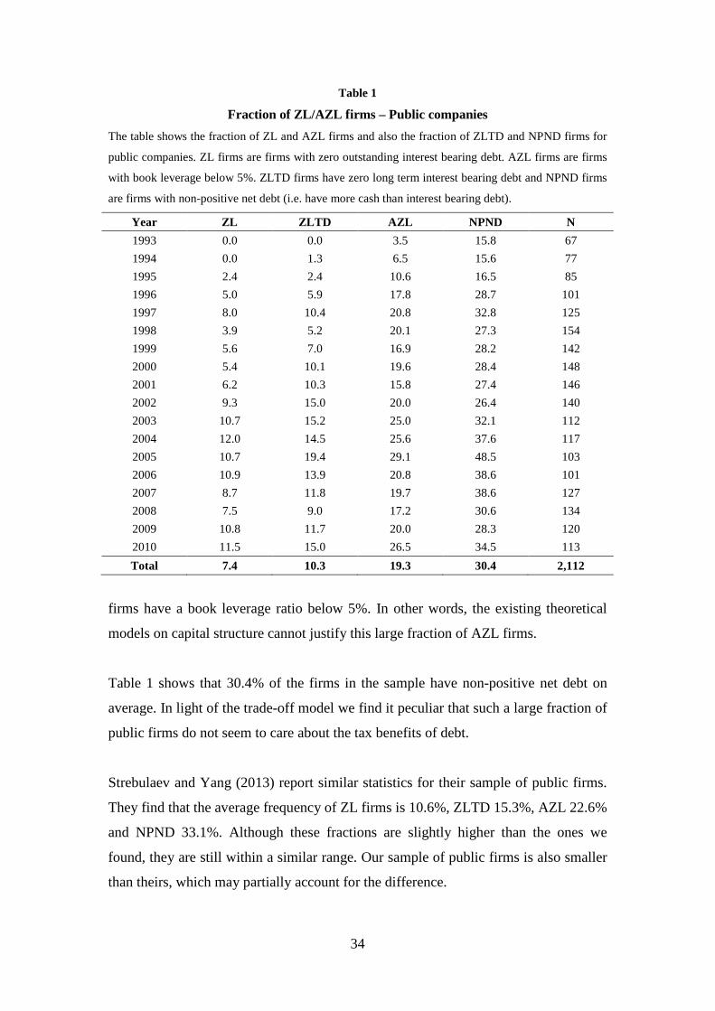
Table 1

Fraction of ZL/AZL firms – Public companies The table shows the fraction of ZL and AZL firms and also the fraction of ZLTD and NPND firms for

public companies. ZL firms are firms with zero outstanding interest bearing debt. AZL firms are firms

with book leverage below 5%. ZLTD firms have zero long term interest bearing debt and NPND firms

are firms with non-positive net debt (i.e. have more cash than interest bearing debt).

Year ZL ZLTD AZL NPND N 1993 0.0 0.0 3.5 15.8 67 1994 0.0 1.3 6.5 15.6 77 1995 2.4 2.4 10.6 16.5 85 1996 5.0 5.9 17.8 28.7 101 1997 8.0 10.4 20.8 32.8 125 1998 3.9 5.2 20.1 27.3 154 1999 5.6 7.0 16.9 28.2 142 2000 5.4 10.1 19.6 28.4 148 2001 6.2 10.3 15.8 27.4 146 2002 9.3 15.0 20.0 26.4 140 2003 10.7 15.2 25.0 32.1 112 2004 12.0 14.5 25.6 37.6 117 2005 10.7 19.4 29.1 48.5 103 2006 10.9 13.9 20.8 38.6 101 2007 8.7 11.8 19.7 38.6 127 2008 7.5 9.0 17.2 30.6 134 2009 10.8 11.7 20.0 28.3 120 2010 11.5 15.0 26.5 34.5 113 Total 7.4 10.3 19.3 30.4 2,112

firms have a book leverage ratio below 5%. In other words, the existing theoretical

models on capital structure cannot justify this large fraction of AZL firms.

Table 1 shows that 30.4% of the firms in the sample have non-positive net debt on

average. In light of the trade-off model we find it peculiar that such a large fraction of

public firms do not seem to care about the tax benefits of debt.

Strebulaev and Yang (2013) report similar statistics for their sample of public firms.

They find that the average frequency of ZL firms is 10.6%, ZLTD 15.3%, AZL 22.6%

and NPND 33.1%. Although these fractions are slightly higher than the ones we

found, they are still within a similar range. Our sample of public firms is also smaller

than theirs, which may partially account for the difference.

34

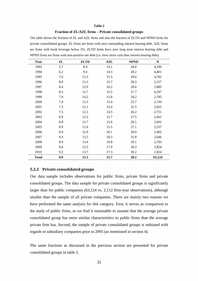
Table 2

Fraction of ZL/AZL firms – Private consolidated groups The table shows the fraction of ZL and AZL firms and also the fraction of ZLTD and NPND firms for

private consolidated groups. ZL firms are firms with zero outstanding interest bearing debt. AZL firms

are firms with book leverage below 5%. ZLTD firms have zero long term interest bearing debt and

NPND firms are firms with non-positive net debt (i.e. have more cash than interest bearing debt).

Year ZL ZLTD AZL NPND N 1993 5.7 8.9 14.1 28.0 4,189 1994 6.2 9.4 14.3 28.2 4,401 1995 7.6 12.3 15.5 28.0 4,762 1996 8.0 12.3 15.7 28.3 5,157 1997 8.4 12.9 16.2 28.6 5,885 1998 8.3 12.7 15.5 27.7 6,297 1999 7.9 14.2 15.8 28.2 2,785 2000 7.4 12.5 15.4 25.7 2,744 2001 7.3 12.1 15.0 25.5 2,825 2002 7.5 12.2 14.5 26.2 2,751 2003 8.9 13.3 15.7 27.5 2,661 2004 8.8 12.7 15.6 28.1 2,601 2005 8.9 12.6 15.5 27.1 2,557 2006 8.9 12.9 16.1 28.9 2,402 2007 9.4 13.5 18.3 31.8 2,646 2008 8.9 13.4 16.8 29.1 2,783 2009 9.6 13.5 17.0 30.3 2,854 2010 9.2 13.7 17.3 30.2 2,824 Total 8.0 12.3 15.7 28.2 63,124

5.2.2 Private consolidated groups

Our data sample includes observations for public firms, private firms and private

consolidated groups. The data sample for private consolidated groups is significantly

larger than for public companies (63,124 vs. 2,112 firm-year observations), although

smaller than the sample of all private companies. There are mainly two reasons we

have performed the same analysis for this category. First, it serves as comparison to

the study of public firms, as we find it reasonable to assume that the average private

consolidated group has more similar characteristics to public firms than the average

private firm has. Second, the sample of private consolidated groups is unbiased with

regards to subsidiary companies prior to 2005 (as mentioned in section 4).

The same fractions as discussed in the previous section are presented for private

consolidated groups in table 2.

35

We observe somewhat similar results as for public companies with an average

fraction of ZL (AZL) firms of 8.0% (15.7%). The average fractions of firms with zero

long-term debt and non-positive net debt are respectively 12.3% and 28.2%.

Comparing table 2 to table 1 we see that the difference across years is far less volatile,

which likely is due to the larger data sample.

5.2.3 Private companies

Since we have access to a large data sample of private companies (345,363 firm-year

observations) we want to perform the same analysis for this group, and check whether

or not there are any differences between public and private firms. To our knowledge

no other study concerning zero leverage has analysed private firms, which, to us,

makes this study more interesting than for public companies. Table 3 reports the

results for private companies.

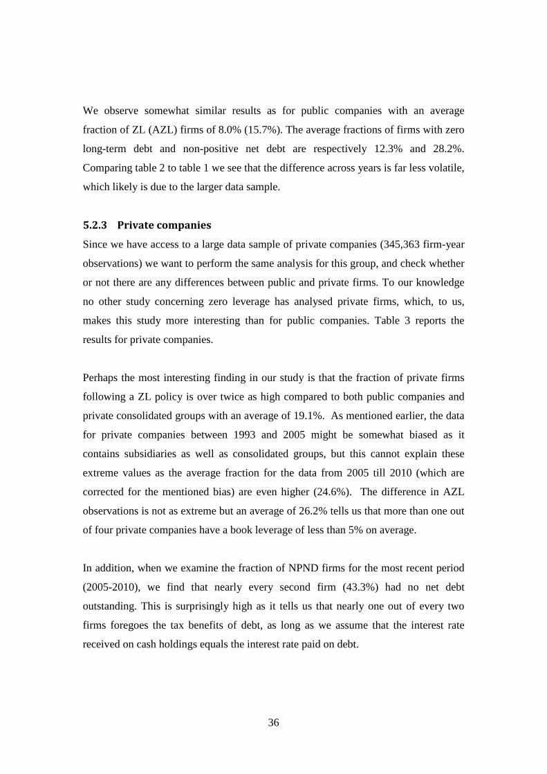
Perhaps the most interesting finding in our study is that the fraction of private firms

following a ZL policy is over twice as high compared to both public companies and

private consolidated groups with an average of 19.1%. As mentioned earlier, the data

for private companies between 1993 and 2005 might be somewhat biased as it

contains subsidiaries as well as consolidated groups, but this cannot explain these

extreme values as the average fraction for the data from 2005 till 2010 (which are

corrected for the mentioned bias) are even higher (24.6%). The difference in AZL

observations is not as extreme but an average of 26.2% tells us that more than one out

of four private companies have a book leverage of less than 5% on average.

In addition, when we examine the fraction of NPND firms for the most recent period

(2005-2010), we find that nearly every second firm (43.3%) had no net debt

outstanding. This is surprisingly high as it tells us that nearly one out of every two

firms foregoes the tax benefits of debt, as long as we assume that the interest rate

received on cash holdings equals the interest rate paid on debt.

36

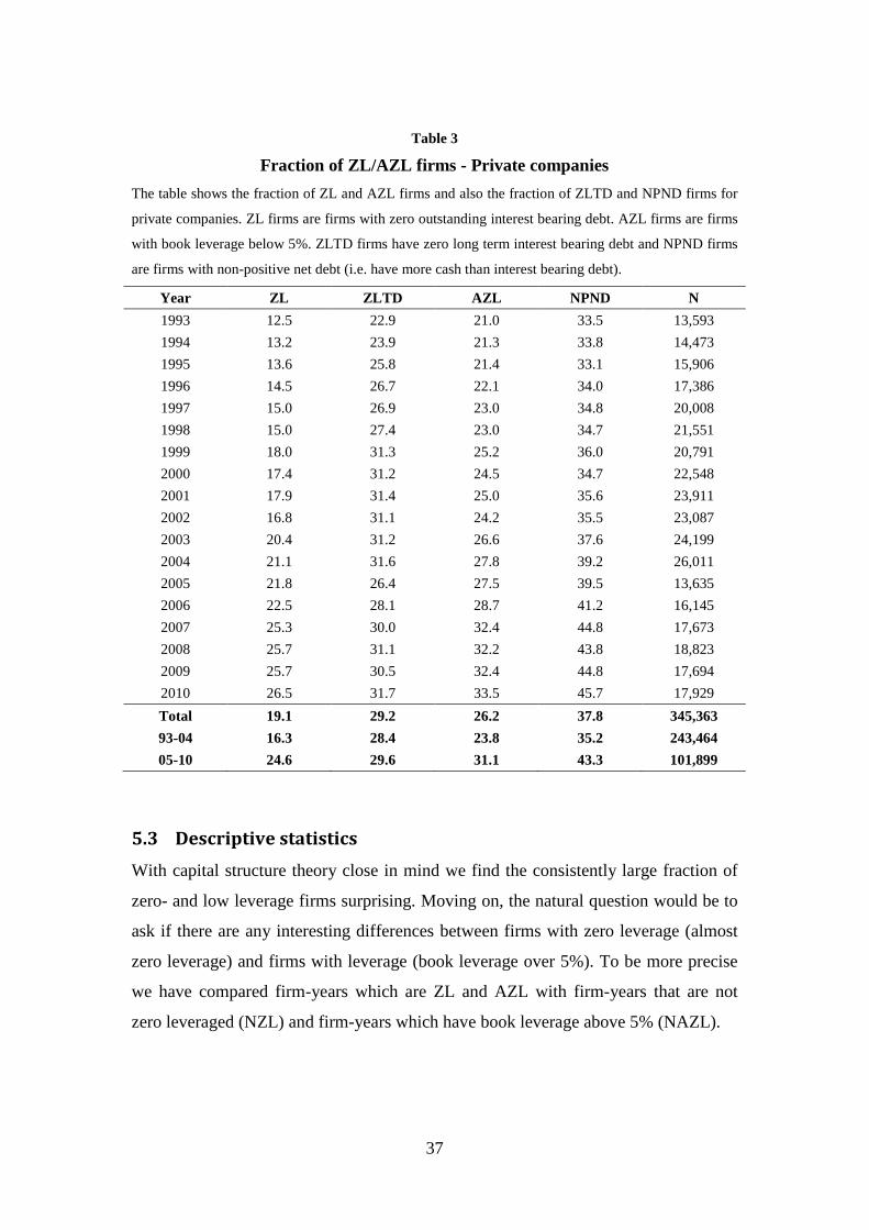
Table 3

Fraction of ZL/AZL firms - Private companies The table shows the fraction of ZL and AZL firms and also the fraction of ZLTD and NPND firms for

private companies. ZL firms are firms with zero outstanding interest bearing debt. AZL firms are firms

with book leverage below 5%. ZLTD firms have zero long term interest bearing debt and NPND firms

are firms with non-positive net debt (i.e. have more cash than interest bearing debt).

Year ZL ZLTD AZL NPND N 1993 12.5 22.9 21.0 33.5 13,593 1994 13.2 23.9 21.3 33.8 14,473 1995 13.6 25.8 21.4 33.1 15,906 1996 14.5 26.7 22.1 34.0 17,386 1997 15.0 26.9 23.0 34.8 20,008 1998 15.0 27.4 23.0 34.7 21,551 1999 18.0 31.3 25.2 36.0 20,791 2000 17.4 31.2 24.5 34.7 22,548 2001 17.9 31.4 25.0 35.6 23,911 2002 16.8 31.1 24.2 35.5 23,087 2003 20.4 31.2 26.6 37.6 24,199 2004 21.1 31.6 27.8 39.2 26,011 2005 21.8 26.4 27.5 39.5 13,635 2006 22.5 28.1 28.7 41.2 16,145 2007 25.3 30.0 32.4 44.8 17,673 2008 25.7 31.1 32.2 43.8 18,823 2009 25.7 30.5 32.4 44.8 17,694 2010 26.5 31.7 33.5 45.7 17,929 Total 19.1 29.2 26.2 37.8 345,363 93-04 16.3 28.4 23.8 35.2 243,464 05-10 24.6 29.6 31.1 43.3 101,899

5.3 Descriptive statistics With capital structure theory close in mind we find the consistently large fraction of

zero- and low leverage firms surprising. Moving on, the natural question would be to

ask if there are any interesting differences between firms with zero leverage (almost

zero leverage) and firms with leverage (book leverage over 5%). To be more precise

we have compared firm-years which are ZL and AZL with firm-years that are not

zero leveraged (NZL) and firm-years which have book leverage above 5% (NAZL).

37

Tables 4, 5 and 6 report a range of descriptive statistics for ZL, AZL, NZL and NAZL

firm-years. For each variable we have conducted a t-test for equality of means where

ZL (AZL) firm-years is one sample and NZL (NAZL) firm-years is the other sample.

In section 5.2 we found the most interesting part of our study to be the sample of

private firms, as this sample had by far the largest portion of zero leveraged

companies. The sample of public firms is quite small, which often makes it difficult to

draw clear conclusions. We will, from now, therefore focus primarily on private firms

and partly private consolidated groups, although we will sometimes still analyse

public firms. Subsequently, from this section (5.3) we have changed the sequence in

which we present the results from the different samples. We will start with describing

private firms (table 4), then private consolidated groups (table 5), and lastly public

firms (table 6). Definitions of all the variables used can be found in appendix 1.

5.3.1 Private companies

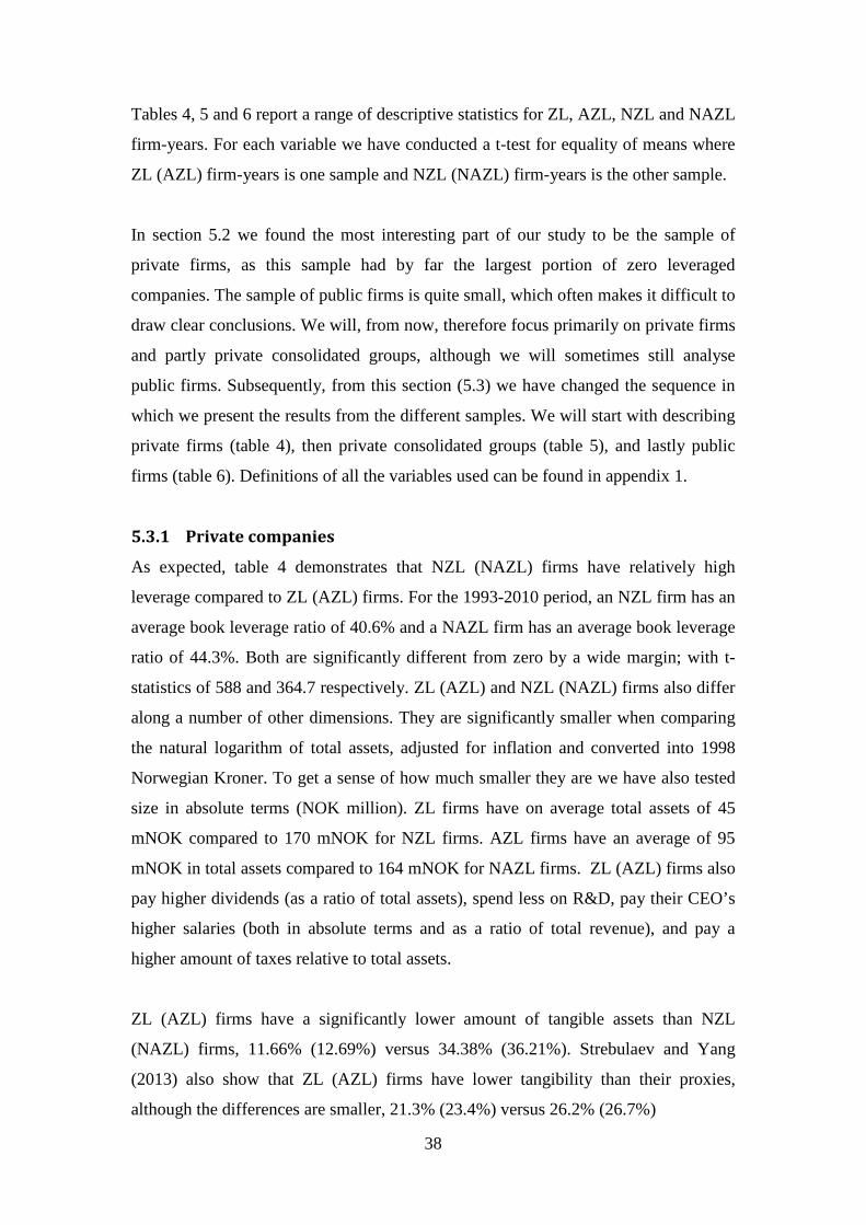
As expected, table 4 demonstrates that NZL (NAZL) firms have relatively high

leverage compared to ZL (AZL) firms. For the 1993-2010 period, an NZL firm has an

average book leverage ratio of 40.6% and a NAZL firm has an average book leverage

ratio of 44.3%. Both are significantly different from zero by a wide margin; with t-

statistics of 588 and 364.7 respectively. ZL (AZL) and NZL (NAZL) firms also differ

along a number of other dimensions. They are significantly smaller when comparing

the natural logarithm of total assets, adjusted for inflation and converted into 1998

Norwegian Kroner. To get a sense of how much smaller they are we have also tested

size in absolute terms (NOK million). ZL firms have on average total assets of 45

mNOK compared to 170 mNOK for NZL firms. AZL firms have an average of 95

mNOK in total assets compared to 164 mNOK for NAZL firms. ZL (AZL) firms also

pay higher dividends (as a ratio of total assets), spend less on R&D, pay their CEO’s

higher salaries (both in absolute terms and as a ratio of total revenue), and pay a

higher amount of taxes relative to total assets.

ZL (AZL) firms have a significantly lower amount of tangible assets than NZL

(NAZL) firms, 11.66% (12.69%) versus 34.38% (36.21%). Strebulaev and Yang

(2013) also show that ZL (AZL) firms have lower tangibility than their proxies,

although the differences are smaller, 21.3% (23.4%) versus 26.2% (26.7%)

38

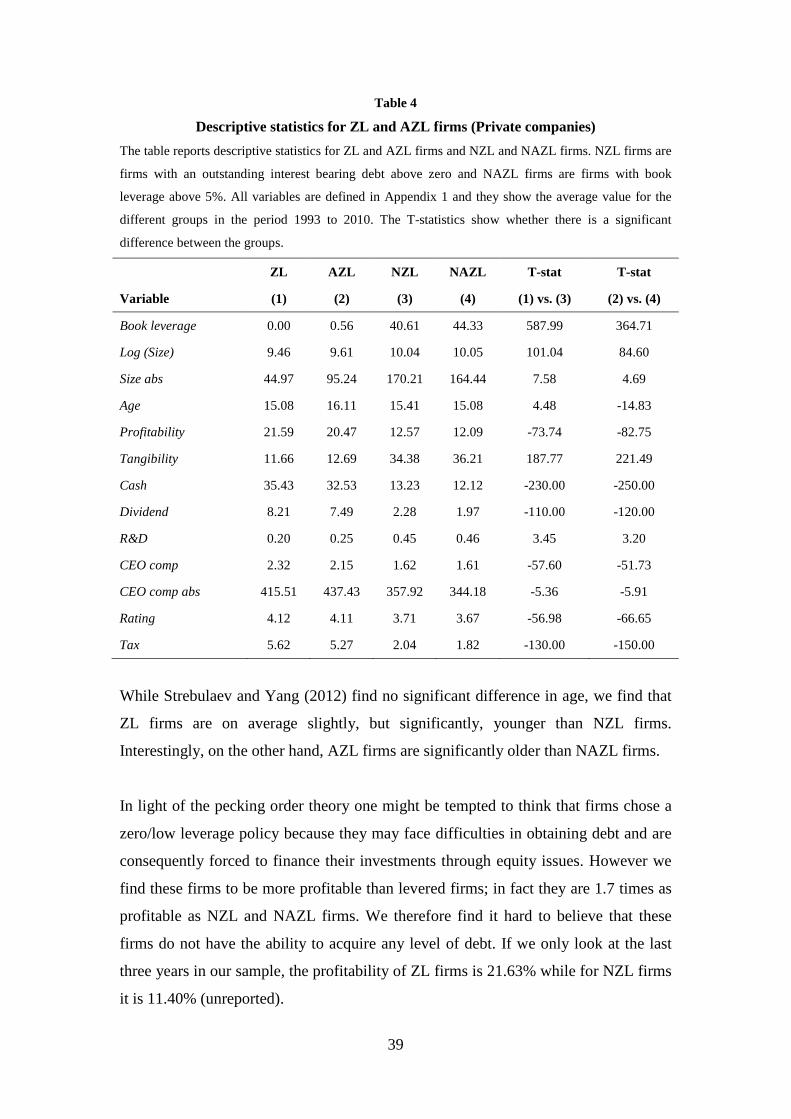
Table 4

Descriptive statistics for ZL and AZL firms (Private companies) The table reports descriptive statistics for ZL and AZL firms and NZL and NAZL firms. NZL firms are

firms with an outstanding interest bearing debt above zero and NAZL firms are firms with book

leverage above 5%. All variables are defined in Appendix 1 and they show the average value for the

different groups in the period 1993 to 2010. The T-statistics show whether there is a significant

difference between the groups.

ZL AZL NZL NAZL T-stat T-stat

Variable (1) (2) (3) (4) (1) vs. (3) (2) vs. (4)

Book leverage 0.00 0.56 40.61 44.33 587.99 364.71

Log (Size) 9.46 9.61 10.04 10.05 101.04 84.60

Size abs 44.97 95.24 170.21 164.44 7.58 4.69

Age 15.08 16.11 15.41 15.08 4.48 -14.83

Profitability 21.59 20.47 12.57 12.09 -73.74 -82.75

Tangibility 11.66 12.69 34.38 36.21 187.77 221.49

Cash 35.43 32.53 13.23 12.12 -230.00 -250.00

Dividend 8.21 7.49 2.28 1.97 -110.00 -120.00

R&D 0.20 0.25 0.45 0.46 3.45 3.20

CEO comp 2.32 2.15 1.62 1.61 -57.60 -51.73

CEO comp abs 415.51 437.43 357.92 344.18 -5.36 -5.91

Rating 4.12 4.11 3.71 3.67 -56.98 -66.65

Tax 5.62 5.27 2.04 1.82 -130.00 -150.00

While Strebulaev and Yang (2012) find no significant difference in age, we find that

ZL firms are on average slightly, but significantly, younger than NZL firms.

Interestingly, on the other hand, AZL firms are significantly older than NAZL firms.

In light of the pecking order theory one might be tempted to think that firms chose a

zero/low leverage policy because they may face difficulties in obtaining debt and are

consequently forced to finance their investments through equity issues. However we

find these firms to be more profitable than levered firms; in fact they are 1.7 times as

profitable as NZL and NAZL firms. We therefore find it hard to believe that these

firms do not have the ability to acquire any level of debt. If we only look at the last

three years in our sample, the profitability of ZL firms is 21.63% while for NZL firms

it is 11.40% (unreported).

39

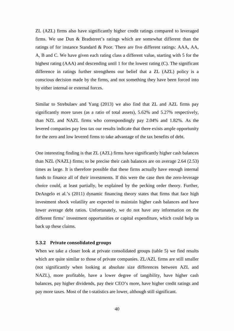
ZL (AZL) firms also have significantly higher credit ratings compared to leveraged

firms. We use Dun & Bradstreet’s ratings which are somewhat different than the

ratings of for instance Standard & Poor. There are five different ratings: AAA, AA,

A, B and C. We have given each rating class a different value, starting with 5 for the

highest rating (AAA) and descending until 1 for the lowest rating (C). The significant

difference in ratings further strengthens our belief that a ZL (AZL) policy is a

conscious decision made by the firms, and not something they have been forced into

by either internal or external forces.

Similar to Strebulaev and Yang (2013) we also find that ZL and AZL firms pay

significantly more taxes (as a ratio of total assets), 5.62% and 5.27% respectively,

than NZL and NAZL firms who correspondingly pay 2.04% and 1.82%. As the

levered companies pay less tax our results indicate that there exists ample opportunity

for the zero and low levered firms to take advantage of the tax benefits of debt.

One interesting finding is that ZL (AZL) firms have significantly higher cash balances

than NZL (NAZL) firms; to be precise their cash balances are on average 2.64 (2.53)

times as large. It is therefore possible that these firms actually have enough internal

funds to finance all of their investments. If this were the case then the zero-leverage

choice could, at least partially, be explained by the pecking order theory. Further,

DeAngelo et al.’s (2011) dynamic financing theory states that firms that face high

investment shock volatility are expected to maintain higher cash balances and have

lower average debt ratios. Unfortunately, we do not have any information on the

different firms’ investment opportunities or capital expenditure, which could help us

back up these claims.

5.3.2 Private consolidated groups

When we take a closer look at private consolidated groups (table 5) we find results

which are quite similar to those of private companies. ZL/AZL firms are still smaller

(not significantly when looking at absolute size differences between AZL and

NAZL), more profitable, have a lower degree of tangibility, have higher cash

balances, pay higher dividends, pay their CEO’s more, have higher credit ratings and

pay more taxes. Most of the t-statistics are lower, although still significant.

40

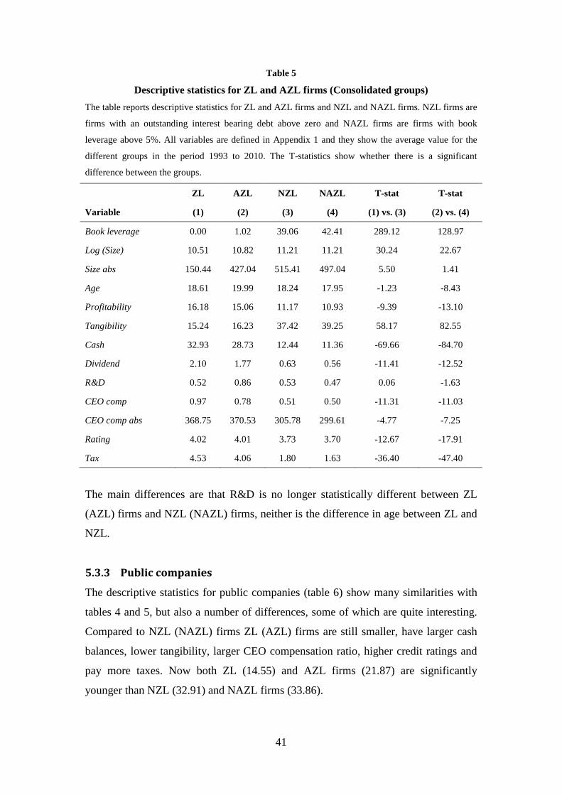
Table 5

Descriptive statistics for ZL and AZL firms (Consolidated groups) The table reports descriptive statistics for ZL and AZL firms and NZL and NAZL firms. NZL firms are

firms with an outstanding interest bearing debt above zero and NAZL firms are firms with book

leverage above 5%. All variables are defined in Appendix 1 and they show the average value for the

different groups in the period 1993 to 2010. The T-statistics show whether there is a significant

difference between the groups.

ZL AZL NZL NAZL T-stat T-stat

Variable (1) (2) (3) (4) (1) vs. (3) (2) vs. (4)

Book leverage 0.00 1.02 39.06 42.41 289.12 128.97

Log (Size) 10.51 10.82 11.21 11.21 30.24 22.67

Size abs 150.44 427.04 515.41 497.04 5.50 1.41

Age 18.61 19.99 18.24 17.95 -1.23 -8.43

Profitability 16.18 15.06 11.17 10.93 -9.39 -13.10

Tangibility 15.24 16.23 37.42 39.25 58.17 82.55

Cash 32.93 28.73 12.44 11.36 -69.66 -84.70

Dividend 2.10 1.77 0.63 0.56 -11.41 -12.52

R&D 0.52 0.86 0.53 0.47 0.06 -1.63

CEO comp 0.97 0.78 0.51 0.50 -11.31 -11.03

CEO comp abs 368.75 370.53 305.78 299.61 -4.77 -7.25

Rating 4.02 4.01 3.73 3.70 -12.67 -17.91

Tax 4.53 4.06 1.80 1.63 -36.40 -47.40

The main differences are that R&D is no longer statistically different between ZL

(AZL) firms and NZL (NAZL) firms, neither is the difference in age between ZL and

NZL.

5.3.3 Public companies

The descriptive statistics for public companies (table 6) show many similarities with

tables 4 and 5, but also a number of differences, some of which are quite interesting.

Compared to NZL (NAZL) firms ZL (AZL) firms are still smaller, have larger cash

balances, lower tangibility, larger CEO compensation ratio, higher credit ratings and

pay more taxes. Now both ZL (14.55) and AZL firms (21.87) are significantly

younger than NZL (32.91) and NAZL firms (33.86).

41

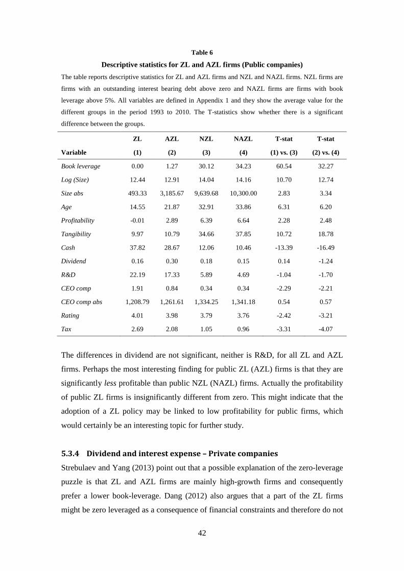
Table 6

Descriptive statistics for ZL and AZL firms (Public companies) The table reports descriptive statistics for ZL and AZL firms and NZL and NAZL firms. NZL firms are

firms with an outstanding interest bearing debt above zero and NAZL firms are firms with book

leverage above 5%. All variables are defined in Appendix 1 and they show the average value for the

different groups in the period 1993 to 2010. The T-statistics show whether there is a significant

difference between the groups.

ZL AZL NZL NAZL T-stat T-stat

Variable (1) (2) (3) (4) (1) vs. (3) (2) vs. (4)

Book leverage 0.00 1.27 30.12 34.23 60.54 32.27

Log (Size) 12.44 12.91 14.04 14.16 10.70 12.74

Size abs 493.33 3,185.67 9,639.68 10,300.00 2.83 3.34

Age 14.55 21.87 32.91 33.86 6.31 6.20

Profitability -0.01 2.89 6.39 6.64 2.28 2.48

Tangibility 9.97 10.79 34.66 37.85 10.72 18.78

Cash 37.82 28.67 12.06 10.46 -13.39 -16.49

Dividend 0.16 0.30 0.18 0.15 0.14 -1.24

R&D 22.19 17.33 5.89 4.69 -1.04 -1.70

CEO comp 1.91 0.84 0.34 0.34 -2.29 -2.21

CEO comp abs 1,208.79 1,261.61 1,334.25 1,341.18 0.54 0.57

Rating 4.01 3.98 3.79 3.76 -2.42 -3.21

Tax 2.69 2.08 1.05 0.96 -3.31 -4.07

The differences in dividend are not significant, neither is R&D, for all ZL and AZL

firms. Perhaps the most interesting finding for public ZL (AZL) firms is that they are

significantly less profitable than public NZL (NAZL) firms. Actually the profitability

of public ZL firms is insignificantly different from zero. This might indicate that the

adoption of a ZL policy may be linked to low profitability for public firms, which

would certainly be an interesting topic for further study.

5.3.4 Dividend and interest expense – Private companies

Strebulaev and Yang (2013) point out that a possible explanation of the zero-leverage

puzzle is that ZL and AZL firms are mainly high-growth firms and consequently

prefer a lower book-leverage. Dang (2012) also argues that a part of the ZL firms

might be zero leveraged as a consequence of financial constraints and therefore do not

42

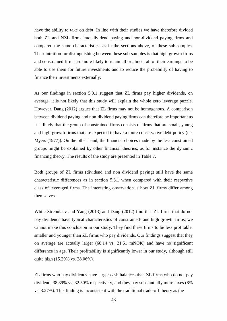
have the ability to take on debt. In line with their studies we have therefore divided

both ZL and NZL firms into dividend paying and non-dividend paying firms and

compared the same characteristics, as in the sections above, of these sub-samples.

Their intuition for distinguishing between these sub-samples is that high growth firms

and constrained firms are more likely to retain all or almost all of their earnings to be

able to use them for future investments and to reduce the probability of having to

finance their investments externally.

As our findings in section 5.3.1 suggest that ZL firms pay higher dividends, on

average, it is not likely that this study will explain the whole zero leverage puzzle.

However, Dang (2012) argues that ZL firms may not be homogenous. A comparison

between dividend paying and non-dividend paying firms can therefore be important as

it is likely that the group of constrained firms consists of firms that are small, young

and high-growth firms that are expected to have a more conservative debt policy (i.e.

Myers (1977)). On the other hand, the financial choices made by the less constrained

groups might be explained by other financial theories, as for instance the dynamic

financing theory. The results of the study are presented in Table 7.

Both groups of ZL firms (dividend and non dividend paying) still have the same

characteristic differences as in section 5.3.1 when compared with their respective

class of leveraged firms. The interesting observation is how ZL firms differ among

themselves.

While Strebulaev and Yang (2013) and Dang (2012) find that ZL firms that do not

pay dividends have typical characteristics of constrained- and high growth firms, we

cannot make this conclusion in our study. They find these firms to be less profitable,

smaller and younger than ZL firms who pay dividends. Our findings suggest that they

on average are actually larger (68.14 vs. 21.51 mNOK) and have no significant

difference in age. Their profitability is significantly lower in our study, although still

quite high (15.20% vs. 28.06%).

ZL firms who pay dividends have larger cash balances than ZL firms who do not pay

dividend, 38.39% vs. 32.50% respectively, and they pay substantially more taxes (8%

vs. 3.27%). This finding is inconsistent with the traditional trade-off theory as the

43

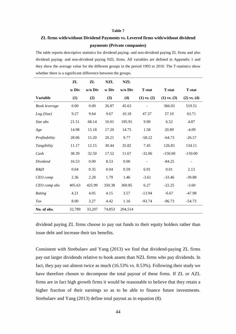
Table 7

ZL firms with/without Dividend Payments vs. Levered firms with/without dividend

payments (Private companies) The table reports descriptive statistics for dividend paying- and non-dividend paying ZL firms and also

dividend paying- and non-dividend paying NZL firms. All variables are defined in Appendix 1 and

they show the average value for the different groups in the period 1993 to 2010. The T-statistics show

whether there is a significant difference between the groups.

ZL ZL NZL NZL

w Div w/o Div w Div w/o Div T-stat T-stat T-stat

Variable (1) (2) (3) (4) (1) vs. (2) (1) vs. (3) (2) vs. (4)

Book leverage 0.00 0.00 26.87 45.63 - 366.03 519.51

Log (Size) 9.27 9.64 9.67 10.18 47.37 57.10 63.71

Size abs 21.51 68.14 10.01 195.91 9.90 6.52 4.87

Age 14.98 15.18 17.20 14.75 1.58 20.89 -4.09

Profitability 28.06 15.20 20.21 9.77 -58.22 -64.73 -26.57

Tangibility 11.17 12.15 30.44 35.82 7.45 126.83 134.11

Cash 38.39 32.50 17.52 11.67 -32.06 -150.00 -150.00

Dividend 16.53 0.00 8.53 0.00 - -84.25 -

R&D 0.04 0.35 0.04 0.59 6.91 0.01 2.13

CEO comp 2.36 2.28 1.79 1.46 -3.61 -33.46 -39.88

CEO comp abs 405.63 425.99 350.38 360.85 6.27 -22.25 -3.60

Rating 4.21 4.05 4.15 3.57 -13.94 -6.67 -47.98

Tax 8.00 3.27 4.42 1.16 -93.74 -96.73 -54.73

No. of obs. 32,789 33,207 74,853 204,514

dividend paying ZL firms choose to pay out funds to their equity holders rather than

issue debt and increase their tax benefits.

Consistent with Strebulaev and Yang (2013) we find that dividend-paying ZL firms

pay out larger dividends relative to book assets than NZL firms who pay dividends. In

fact, they pay out almost twice as much (16.53% vs. 8.53%). Following their study we

have therefore chosen to decompose the total payout of these firms. If ZL or AZL

firms are in fact high growth firms it would be reasonable to believe that they retain a

higher fraction of their earnings so as to be able to finance future investments.

Strebulaev and Yang (2013) define total payout as in equation (8).

44

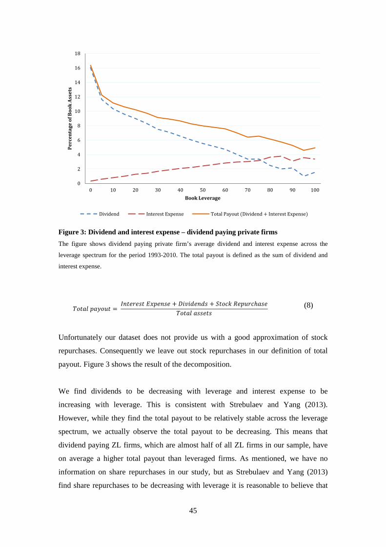
Figure 3: Dividend and interest expense – dividend paying private firms The figure shows dividend paying private firm’s average dividend and interest expense across the

leverage spectrum for the period 1993-2010. The total payout is defined as the sum of dividend and

interest expense.

𝑇𝑜𝑡𝑎𝑙 𝑝𝑎𝑦𝑜𝑢𝑡 = 𝐼𝑛𝑡𝑒𝑟𝑒𝑠𝑡 𝐸𝑥𝑝𝑒𝑛𝑠𝑒 + 𝐷𝑖𝑣𝑖𝑑𝑒𝑛𝑑𝑠 + 𝑆𝑡𝑜𝑐𝑘 𝑅𝑒𝑝𝑢𝑟𝑐ℎ𝑎𝑠𝑒

𝑇𝑜𝑡𝑎𝑙 𝑎𝑠𝑠𝑒𝑡𝑠 (8)

Unfortunately our dataset does not provide us with a good approximation of stock

repurchases. Consequently we leave out stock repurchases in our definition of total

payout. Figure 3 shows the result of the decomposition.

We find dividends to be decreasing with leverage and interest expense to be

increasing with leverage. This is consistent with Strebulaev and Yang (2013).

However, while they find the total payout to be relatively stable across the leverage

spectrum, we actually observe the total payout to be decreasing. This means that

dividend paying ZL firms, which are almost half of all ZL firms in our sample, have

on average a higher total payout than leveraged firms. As mentioned, we have no

information on share repurchases in our study, but as Strebulaev and Yang (2013)

find share repurchases to be decreasing with leverage it is reasonable to believe that

0

2

4

6

8

10

12

14

16

18

0 10 20 30 40 50 60 70 80 90 100

Perc

enta

ge o

f Boo

k As

sets

Book Leverage

Dividend Interest Expenxe Total Payout (Dividend + Interest Expense)

45

such an inclusion would make the slope of the total payout even steeper. This is an

interesting finding because it indicates that dividend paying ZL and AZL firms do not

choose lower debt levels in order to be able to retain a higher fraction of their

earnings. In other words, it seems that dynamic financing models cannot explain the

zero leverage puzzle for these firms, as they would explain zero leverage as a

consequence of a company’s wish to retain a higher proportion of its earnings to be

able to finance future investments.

5.4 Industry To get a better understanding of zero-leverage behaviour it might be interesting to

take a closer look at differences between the industries the companies operate in. Our

dataset provides NACE classifications for all the firm-year observations, which makes

it possible for us to do so. In addition to general NACE classifications the data is also

sorted into 12 main industries. We have decided to use this main classification in our

industry study, which is presented in table 9. For a better understanding of which

NACE classifications are included in the 12 different industries, please see Appendix

2.

Table 8 reports the distribution of ZL and AZL firms in addition to the average book

leverage (BL) and the average firm size (in mNOK) of each industry. Table 9 shows a

considerable variation in the distribution of ZL/AZL firms between the industries,

which can indicate that industry specific factors might explain parts of the zero

leverage puzzle. The ZL (AZL) distribution ranges from 9.2% (12.9%) in Primary

industries to 45.9% (60.4%) in Financial services. IT/Telecom and Culture/Media

have the second and third highest distribution of ZL firms. Strebulaev and Yang

(2013) point out that reputation, human capital and asset illiquidity considerations

might be influential in the explanation of ZL behaviour in these industries.

Given that the average firm size in the financial services sector is as high as 1,224

mNOK, the second largest of the 12 industries, we found it somewhat surprising that

this industry had by far the highest proportion of ZL firms, particularly since our

previous findings show that ZL firms are significantly smaller than leveraged firms.

We therefore examined the different firms within this industry, and found that only a

46

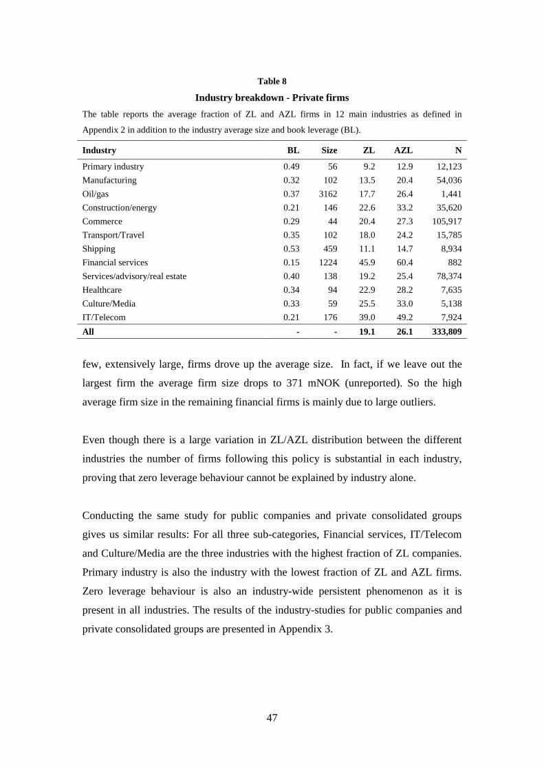
Table 8

Industry breakdown - Private firms The table reports the average fraction of ZL and AZL firms in 12 main industries as defined in

Appendix 2 in addition to the industry average size and book leverage (BL).

Industry BL Size ZL AZL N

Primary industry 0.49 56 9.2 12.9 12,123 Manufacturing 0.32 102 13.5 20.4 54,036 Oil/gas 0.37 3162 17.7 26.4 1,441 Construction/energy 0.21 146 22.6 33.2 35,620 Commerce 0.29 44 20.4 27.3 105,917 Transport/Travel 0.35 102 18.0 24.2 15,785 Shipping 0.53 459 11.1 14.7 8,934 Financial services 0.15 1224 45.9 60.4 882 Services/advisory/real estate 0.40 138 19.2 25.4 78,374 Healthcare 0.34 94 22.9 28.2 7,635 Culture/Media 0.33 59 25.5 33.0 5,138 IT/Telecom 0.21 176 39.0 49.2 7,924 All - - 19.1 26.1 333,809

few, extensively large, firms drove up the average size. In fact, if we leave out the

largest firm the average firm size drops to 371 mNOK (unreported). So the high

average firm size in the remaining financial firms is mainly due to large outliers.

Even though there is a large variation in ZL/AZL distribution between the different

industries the number of firms following this policy is substantial in each industry,

proving that zero leverage behaviour cannot be explained by industry alone.

Conducting the same study for public companies and private consolidated groups

gives us similar results: For all three sub-categories, Financial services, IT/Telecom

and Culture/Media are the three industries with the highest fraction of ZL companies.

Primary industry is also the industry with the lowest fraction of ZL and AZL firms.

Zero leverage behaviour is also an industry-wide persistent phenomenon as it is

present in all industries. The results of the industry-studies for public companies and

private consolidated groups are presented in Appendix 3.

47

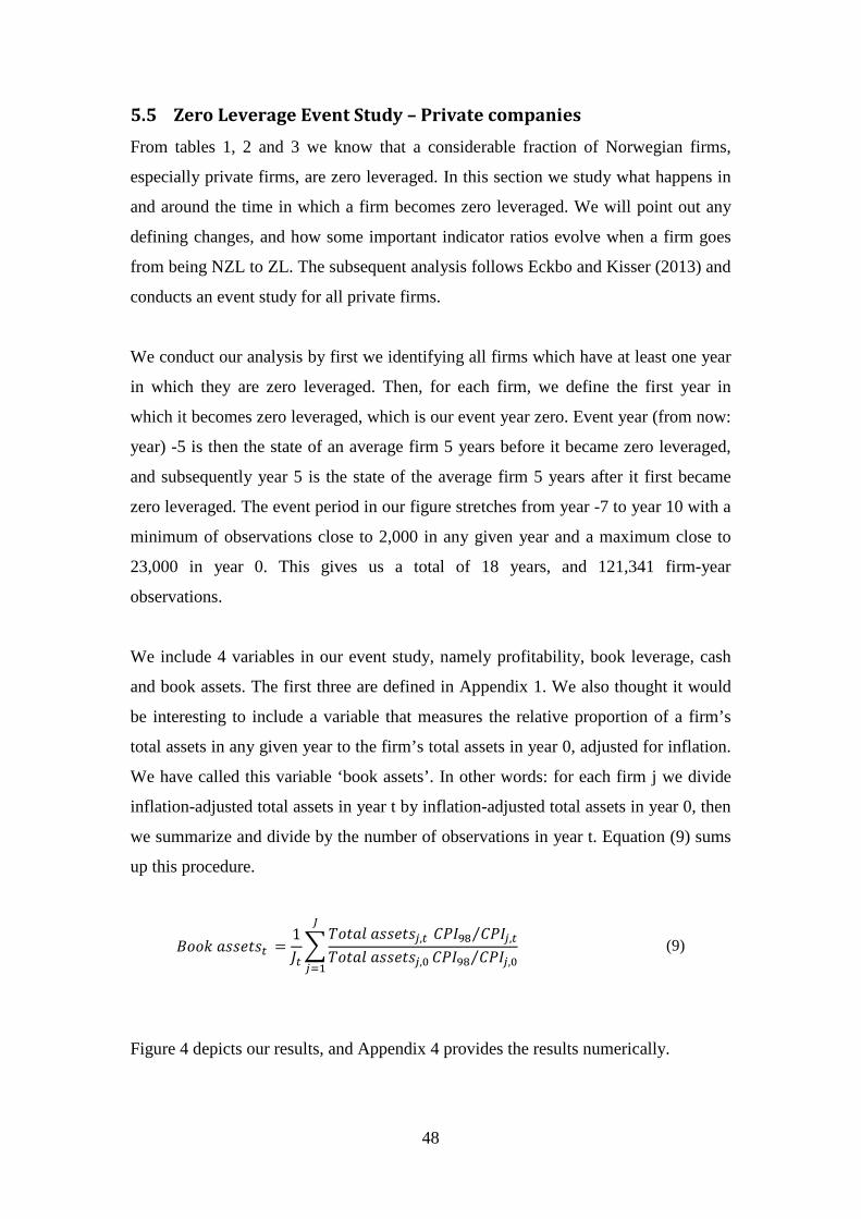
5.5 Zero Leverage Event Study – Private companies From tables 1, 2 and 3 we know that a considerable fraction of Norwegian firms,

especially private firms, are zero leveraged. In this section we study what happens in

and around the time in which a firm becomes zero leveraged. We will point out any

defining changes, and how some important indicator ratios evolve when a firm goes

from being NZL to ZL. The subsequent analysis follows Eckbo and Kisser (2013) and

conducts an event study for all private firms.

We conduct our analysis by first we identifying all firms which have at least one year

in which they are zero leveraged. Then, for each firm, we define the first year in

which it becomes zero leveraged, which is our event year zero. Event year (from now:

year) -5 is then the state of an average firm 5 years before it became zero leveraged,

and subsequently year 5 is the state of the average firm 5 years after it first became

zero leveraged. The event period in our figure stretches from year -7 to year 10 with a

minimum of observations close to 2,000 in any given year and a maximum close to

23,000 in year 0. This gives us a total of 18 years, and 121,341 firm-year

observations.

We include 4 variables in our event study, namely profitability, book leverage, cash

and book assets. The first three are defined in Appendix 1. We also thought it would

be interesting to include a variable that measures the relative proportion of a firm’s

total assets in any given year to the firm’s total assets in year 0, adjusted for inflation.

We have called this variable ‘book assets’. In other words: for each firm j we divide

inflation-adjusted total assets in year t by inflation-adjusted total assets in year 0, then

we summarize and divide by the number of observations in year t. Equation (9) sums

up this procedure.

𝐵𝑜𝑜𝑘 𝑎𝑠𝑠𝑒𝑡𝑠𝑡 =1𝐽𝑡�

𝑇𝑜𝑡𝑎𝑙 𝑎𝑠𝑠𝑒𝑡𝑠𝑗,𝑡 𝐶𝑃𝐼98 𝐶𝑃𝐼𝑗,𝑡⁄𝑇𝑜𝑡𝑎𝑙 𝑎𝑠𝑠𝑒𝑡𝑠𝑗,0 𝐶𝑃𝐼98 𝐶𝑃𝐼𝑗,0⁄

𝐽

𝑗=1

(9)

Figure 4 depicts our results, and Appendix 4 provides the results numerically.

48

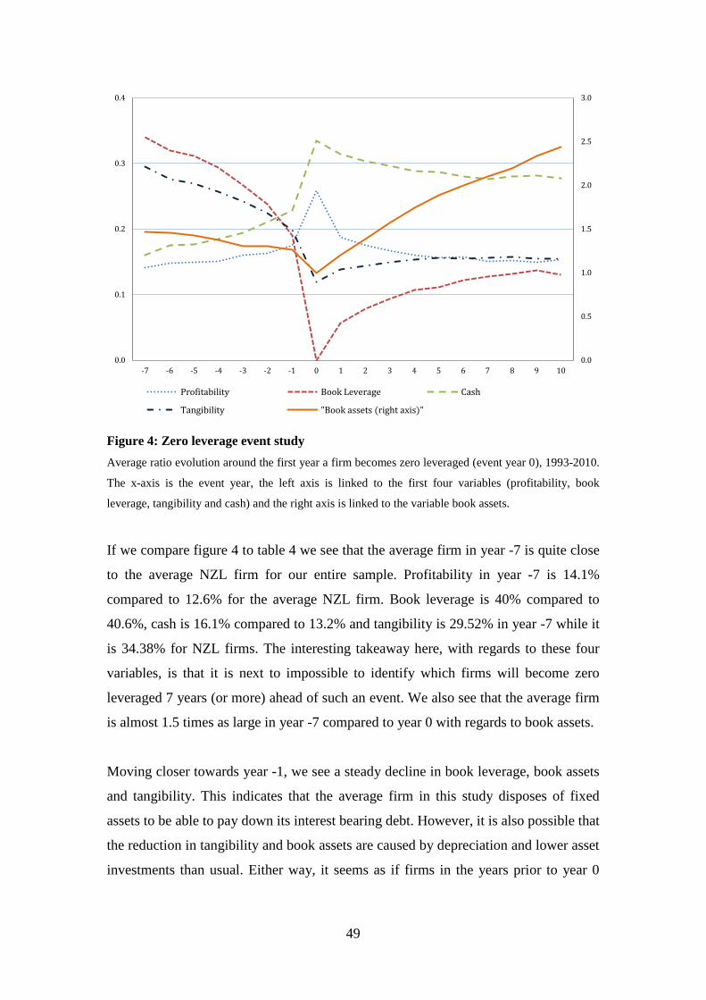
Figure 4: Zero leverage event study Average ratio evolution around the first year a firm becomes zero leveraged (event year 0), 1993-2010.

The x-axis is the event year, the left axis is linked to the first four variables (profitability, book

leverage, tangibility and cash) and the right axis is linked to the variable book assets.

If we compare figure 4 to table 4 we see that the average firm in year -7 is quite close

to the average NZL firm for our entire sample. Profitability in year -7 is 14.1%

compared to 12.6% for the average NZL firm. Book leverage is 40% compared to

40.6%, cash is 16.1% compared to 13.2% and tangibility is 29.52% in year -7 while it

is 34.38% for NZL firms. The interesting takeaway here, with regards to these four

variables, is that it is next to impossible to identify which firms will become zero

leveraged 7 years (or more) ahead of such an event. We also see that the average firm

is almost 1.5 times as large in year -7 compared to year 0 with regards to book assets.

Moving closer towards year -1, we see a steady decline in book leverage, book assets

and tangibility. This indicates that the average firm in this study disposes of fixed

assets to be able to pay down its interest bearing debt. However, it is also possible that

the reduction in tangibility and book assets are caused by depreciation and lower asset

investments than usual. Either way, it seems as if firms in the years prior to year 0

0.0

0.5

1.0

1.5

2.0

2.5

3.0

0.0

0.1

0.2

0.3

0.4

-7 -6 -5 -4 -3 -2 -1 0 1 2 3 4 5 6 7 8 9 10

Profitability Book Leverage Cash

Tangibility "Book assets (right axis)"

49

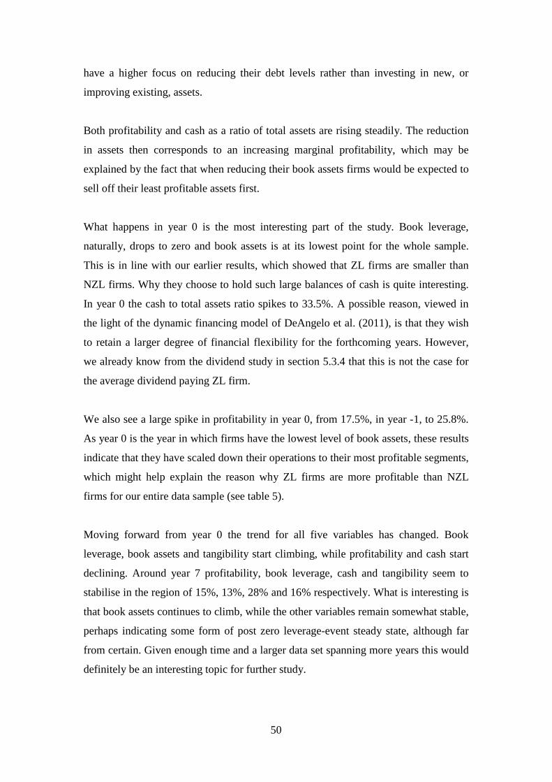
have a higher focus on reducing their debt levels rather than investing in new, or

improving existing, assets.

Both profitability and cash as a ratio of total assets are rising steadily. The reduction

in assets then corresponds to an increasing marginal profitability, which may be

explained by the fact that when reducing their book assets firms would be expected to

sell off their least profitable assets first.

What happens in year 0 is the most interesting part of the study. Book leverage,

naturally, drops to zero and book assets is at its lowest point for the whole sample.

This is in line with our earlier results, which showed that ZL firms are smaller than

NZL firms. Why they choose to hold such large balances of cash is quite interesting.

In year 0 the cash to total assets ratio spikes to 33.5%. A possible reason, viewed in

the light of the dynamic financing model of DeAngelo et al. (2011), is that they wish

to retain a larger degree of financial flexibility for the forthcoming years. However,

we already know from the dividend study in section 5.3.4 that this is not the case for

the average dividend paying ZL firm.

We also see a large spike in profitability in year 0, from 17.5%, in year -1, to 25.8%.

As year 0 is the year in which firms have the lowest level of book assets, these results

indicate that they have scaled down their operations to their most profitable segments,

which might help explain the reason why ZL firms are more profitable than NZL

firms for our entire data sample (see table 5).

Moving forward from year 0 the trend for all five variables has changed. Book

leverage, book assets and tangibility start climbing, while profitability and cash start

declining. Around year 7 profitability, book leverage, cash and tangibility seem to

stabilise in the region of 15%, 13%, 28% and 16% respectively. What is interesting is

that book assets continues to climb, while the other variables remain somewhat stable,

perhaps indicating some form of post zero leverage-event steady state, although far

from certain. Given enough time and a larger data set spanning more years this would

definitely be an interesting topic for further study.

50

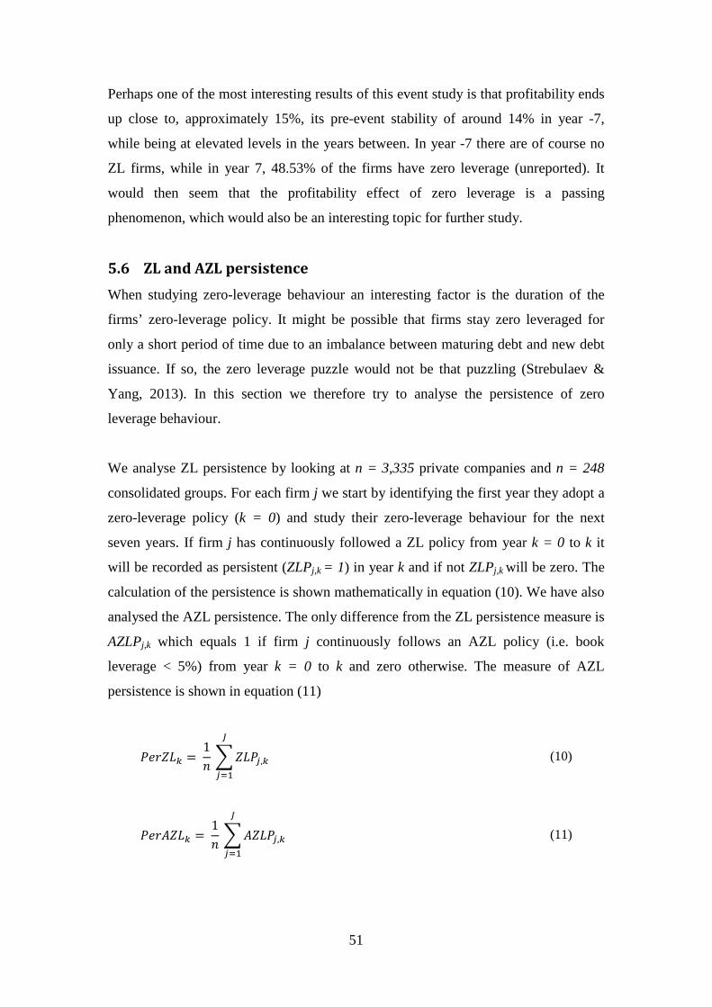
Perhaps one of the most interesting results of this event study is that profitability ends

up close to, approximately 15%, its pre-event stability of around 14% in year -7,

while being at elevated levels in the years between. In year -7 there are of course no

ZL firms, while in year 7, 48.53% of the firms have zero leverage (unreported). It

would then seem that the profitability effect of zero leverage is a passing

phenomenon, which would also be an interesting topic for further study.

5.6 ZL and AZL persistence When studying zero-leverage behaviour an interesting factor is the duration of the

firms’ zero-leverage policy. It might be possible that firms stay zero leveraged for

only a short period of time due to an imbalance between maturing debt and new debt

issuance. If so, the zero leverage puzzle would not be that puzzling (Strebulaev &

Yang, 2013). In this section we therefore try to analyse the persistence of zero

leverage behaviour.

We analyse ZL persistence by looking at n = 3,335 private companies and n = 248

consolidated groups. For each firm j we start by identifying the first year they adopt a

zero-leverage policy (k = 0) and study their zero-leverage behaviour for the next

seven years. If firm j has continuously followed a ZL policy from year k = 0 to k it

will be recorded as persistent (ZLPj,k = 1) in year k and if not ZLPj,k will be zero. The

calculation of the persistence is shown mathematically in equation (10). We have also

analysed the AZL persistence. The only difference from the ZL persistence measure is

AZLPj,k which equals 1 if firm j continuously follows an AZL policy (i.e. book

leverage < 5%) from year k = 0 to k and zero otherwise. The measure of AZL

persistence is shown in equation (11)

𝑃𝑒𝑟𝑍𝐿𝑘 = 1𝑛

�𝑍𝐿𝑃𝑗,𝑘

𝐽

𝑗=1

(10)

𝑃𝑒𝑟𝐴𝑍𝐿𝑘 = 1𝑛

�𝐴𝑍𝐿𝑃𝑗,𝑘

𝐽

𝑗=1

(11)

51

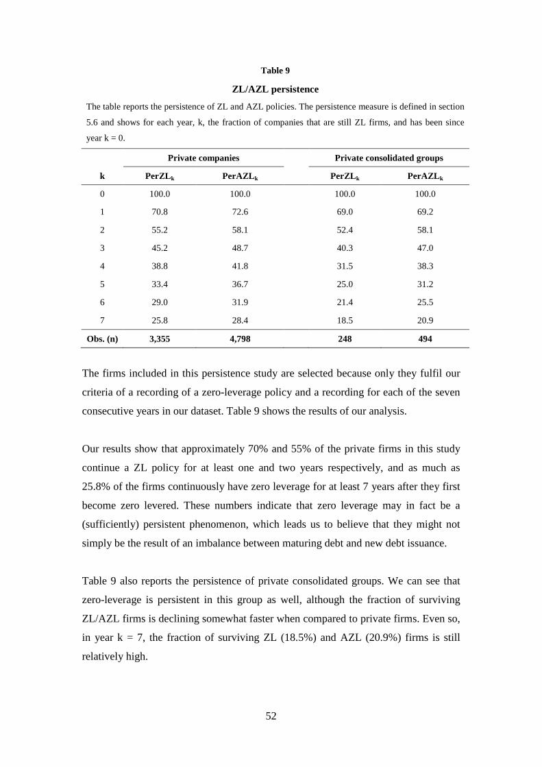
Table 9

ZL/AZL persistence The table reports the persistence of ZL and AZL policies. The persistence measure is defined in section

5.6 and shows for each year, k, the fraction of companies that are still ZL firms, and has been since

year k = 0.

Private companies Private consolidated groups

k PerZLk PerAZLk PerZLk PerAZLk

0 100.0 100.0 100.0 100.0

1 70.8 72.6 69.0 69.2

2 55.2 58.1 52.4 58.1

3 45.2 48.7 40.3 47.0

4 38.8 41.8 31.5 38.3

5 33.4 36.7 25.0 31.2

6 29.0 31.9 21.4 25.5

7 25.8 28.4 18.5 20.9

Obs. (n) 3,355 4,798 248 494

The firms included in this persistence study are selected because only they fulfil our

criteria of a recording of a zero-leverage policy and a recording for each of the seven

consecutive years in our dataset. Table 9 shows the results of our analysis.

Our results show that approximately 70% and 55% of the private firms in this study

continue a ZL policy for at least one and two years respectively, and as much as

25.8% of the firms continuously have zero leverage for at least 7 years after they first

become zero levered. These numbers indicate that zero leverage may in fact be a

(sufficiently) persistent phenomenon, which leads us to believe that they might not

simply be the result of an imbalance between maturing debt and new debt issuance.

Table 9 also reports the persistence of private consolidated groups. We can see that

zero-leverage is persistent in this group as well, although the fraction of surviving

ZL/AZL firms is declining somewhat faster when compared to private firms. Even so,

in year k = 7, the fraction of surviving ZL (18.5%) and AZL (20.9%) firms is still

relatively high.

52

5.7 Logistic Regression Analysis Table 10 contains the results of our logistic regression analysis. The reported

coefficients are the average partial effect of each variable, with standard errors in

parentheses. The number of stars reports the level of significance; three being

significant at the 1% level, two at 5%, one at 10% and no stars insignificance. The

dependent variable is a dummy variable for ZL, which takes the value of 1 if a firm-

year observation has zero outstanding debt and 0 otherwise. For each of our three

samples we have two subsamples, the first ones including six independent variables:

size, profitability, cash, age, tangibility and initial ZL. In the second subsamples we

have added three more variables: R&D, CEO compensation and industry fraction of

ZL.

Overall the results show that the regressions are statistically significant, with pseudo

R-squared ranging from 0.377 to 0.512. The coefficient on firm size is significantly

negative in models 1-5, with values ranging from -0.005 to -0.015. In model 6 the size

coefficient is insignificantly negative; this may be due to the smaller sample size of

this model. These results strongly indicate that a firm is more likely to adopt a ZL

policy when it is smaller, which is in line with our descriptive statistics (see table 4 –

6).

Profitability is significantly positive at the 1% level for models 1-3, at the 5% level

for model 4, and positive, but not significant, for models 5 and 6. So the more

profitable a firm is the more likely it is to be zero leveraged, at least for private

companies and private consolidated groups. To explore this relationship further we

have also looked at the interaction between profitability and size. For private

companies we conducted a fixed effects linear regression with profitability as the

dependent variable and log (size) as an independent variable. We conducted the same

regression for private consolidated groups, but with random effects instead of fixed2.

Both regressions revealed a significant negative relationship between size and

profitability with coefficients for both sub-samples around -0,01 (unreported). This

means that the difference in profitability between ZL and NZL firms for private firms

and private consolidated groups might be a consequence of this negative relationship

2 The choice between fixed and random effects was done by running a Hausman test

53

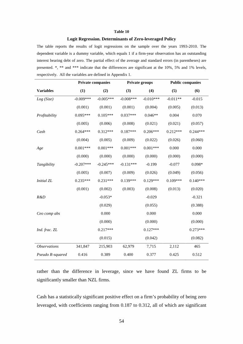
Table 10

Logit Regression. Determinants of Zero-leveraged Policy The table reports the results of logit regressions on the sample over the years 1993-2010. The

dependent variable is a dummy variable, which equals 1 if a firm-year observation has an outstanding

interest bearing debt of zero. The partial effect of the average and standard errors (in parentheses) are

presented. *, ** and *** indicate that the differences are significant at the 10%, 5% and 1% levels,

respectively. All the variables are defined in Appendix 1. Private companies Private groups Public companies

Variables (1) (2) (3) (4) (5) (6)

Log (Size) -0.009*** -0.005*** -0.008*** -0.010*** -0.011** -0.015

(0.001) (0.001) (0.001) (0.004) (0.005) (0.013)

Profitability 0.095*** 0.105*** 0.037*** 0.046** 0.004 0.070

(0.005) (0.006) (0.008) (0.021) (0.021) (0.057)

Cash 0.264*** 0.312*** 0.187*** 0.206*** 0.212*** 0.244***

(0.004) (0.005) (0.009) (0.022) (0.026) (0.060)

Age 0.001*** 0.001*** 0.001*** 0.001*** 0.000 0.000

(0.000) (0.000) (0.000) (0.000) (0.000) (0.000)

Tangibility -0.207*** -0.245*** -0.131*** -0.199 -0.077 0.098*

(0.005) (0.007) (0.009) (0.026) (0.049) (0.056)

Initial ZL 0.235*** 0.231*** 0.139*** 0.129*** 0.109*** 0.140***

(0.001) (0.002) (0.003) (0.008) (0.013) (0.020)

R&D

-0.053*

-0.029

-0.321

(0.029)

(0.055)

(0.388)

Ceo comp abs 0.000

0.000

0.000

(0.000)

(0.000)

(0.000)

Ind. frac. ZL 0.217***

0.127***

0.273***

(0.015) (0.042) (0.082)

Observations 341,847 215,903 62,979 7,715 2,112 465

Pseudo R-squared 0.416 0.389 0.400 0.377 0.425 0.512

rather than the difference in leverage, since we have found ZL firms to be

significantly smaller than NZL firms.

Cash has a statistically significant positive effect on a firm’s probability of being zero

leveraged, with coefficients ranging from 0.187 to 0.312, all of which are significant

54

at the 1% level. Regarding age, all the coefficients are marginally positive and

statistically significant (except for model 5). Cash is the independent variable with

coefficients of the largest magnitude, meaning that the marginal effect of cash is

larger than any of the other variables. The larger the cash holdings of a firm the larger

the probability of that firm being a ZL firm, which is consistent with our earlier

results in tables 4, 5 and 6.

The age coefficients, on the other hand, are of the smallest magnitude, but they are

still significant, and positive, for all models except models 5 and 6. The age

coefficients in models 1-4 are in line with our earlier results. The older a private firm

is the more likely it is to be zero leveraged, although the effect is very small. As we

can see from tables 4, 5 and 6, the age gap between ZL and NZL firms is existent, but

minor.

Tangibility is significantly negative at the 1% level for models 1-3, significantly

positive at the 10% level for model 6, and insignificantly negative for models 4 and 5.

The coefficient values for the models range from -0.245 (model 2) to 0.098 (model 6).

So a firm with fewer tangible assets is more likely to be a ZL firm, except in model 6.

The coefficients for the variable initial ZL (if a firm is a ZL firm in its first firm-year

observation) are all significantly positive, and of a large magnitude, at the 1% level

for all six models. A firm which is zero leveraged the first time it is reported in our

dataset is then more likely to be zero leveraged in subsequent years, which supports

our findings from our persistence study.

As previously mentioned, we added three more variables in models 2, 4 and 6, namely

R&D, CEO compensation and industry fraction of ZL. As we can see from table 10

R&D is negative in all models, but insignificant in models 4 and 6, and only

significant at the 10% level in model 2. This is consistent with our descriptive study,

where we found that ZL firms spend less on R&D than NZL firms.

The coefficients for CEO compensation are not significant for any of the models, and

they are also of a very low magnitude.

55

Lastly, the coefficients of the variable for industry fraction of ZL are significantly

positive at the 1% level for all three models, and they are of a large scale. A firm is

then more likely to be zero leveraged if the fraction of firms within its NACE-coded

industry is high.

All in all comparing the results from our logistic regression with our descriptive study

in section 5.3, we find that they support each other nicely, and we can largely draw

similar conclusions from both.

56

6 Concluding remarks

In this thesis we have documented the puzzling fact of Norwegian firms’ propensity

to have zero outstanding debt. Using publicly available accounting data over the

period 1993-2010, collected and provided by SNF (Institute for Research in

Economics and Business Administration), we have analysed all Norwegian firms,

both public and private.

To our knowledge there are few similar studies regarding Norwegian firms, and little

theoretical and empirical research into the fact that firms choose to have zero

outstanding debt despite the existence of the tax deductibility of interest payments.

We therefore hope that this paper can help shed light on the zero leveraged mystery,

and perhaps inspire others to expand and continue our chosen research path.

We begin our analysis by studying both private and public firms. Then we choose to

focus primarily on private firms. There are two main reasons behind this choice. First,

there are few publicly listed companies in Norway, which makes the sample size

small, while on the other hand our sample size of private firms is extensive. Second,

zero leverage is a more prevalent phenomenon for private firms, and thus the results

from our analysis of this sample are, to us (and hopefully the reader), of greater

interest.

We find that 19.1% of all private firms have zero outstanding debt over the whole

period, which is twice the rate of public firms, and 29.2% have less than 5% book

leverage, thrice the rate of public firms. Compared with leveraged firms, zero

leveraged firms are smaller, more profitable, have larger cash balances, pay more

dividends, have higher credit ratings, more tangible assets and they pay more taxes.

In the years leading up to the year in which firms become zero leveraged they show

increasing profitability and cash holdings, and decreasing total assets and book

leverage. The trends are reversed in the years following the zero leverage event-year.

Firms are at their most profitable (by a large margin), have largest cash holdings and

the smallest amount of total assets in the year they become zero leveraged.

57

We find that zero leveraged firms can be divided into two main categories, namely

dividend payers and non-dividend payers. ZL firms who pay dividends are smaller,

more profitable, have larger cash holding and pay more taxes than ZL firms who do

not pay dividends. Further, our analysis suggests that zero leverage policy may be

persistent, with almost 26% of zero leveraged firms refraining from debt for at least

eight consecutive years.

Further studies into the zero leverage mystery would certainly be interesting. Given

more time and experience we would have liked to incorporate proxy firms in our

analysis as we believe it could help to shed even more light on the extreme corporate

financial policy of zero outstanding debt. We would also have liked to have included

market values and share repurchases in our study, and if available we believe such

data can provide further empirical evidence, and possibly explanations, into the zero

leverage mystery. Although a daunting task, we believe cross-national studies

examining the zero leverage phenomenon could be very insightful and add to the

small, but growing, literature of such an interesting field within corporate finance.

58

7 References

Aldrich, J. H. Nelson, F. D. 1984. Linear Probability, Logit, and Probit Models. Sage

Publications (Beverly Hills).

Berk, J. DeMarzo, P. 2011. Corporate Finance (second edition). Pearson Education.

Dang, V. A. 2012. An Empirical Analysis of Zero-Leverage Firms: New Evidence

From the UK. Manchester Business School Research Paper No. 584.

DeAngelo, H. DeAngelo, L. Whited, T. 2011. Capital Structure Dynamics and

Transitory Debt. Journal of Financial Economics, vol. 99, pp. 235-261.

Eckbo, B. E. Kisser, M. 2012. Corporate Funding: Who Finances Externally. Tuck

School of Business Working Paper No. 2012-110.

Fama, E. French, K. 2002. Testing Trade-off and Pecking Order Predictions About

Dividends and Debt. The Review of Financial Studies, vol. 15 (1), pp. 1-33.

Fama, E. French, K. 2005. Financing Decisions: Who Issues Stock? Journal of

Financial Economics, vol. 76 (3), pp. 549-582.

Fischer, E. O. Heinkel, R. Zechner, J. 1989. Dynamic Capital Structure Choice:

Theory and Tests. The Journal of Finance, vol. 44 (1), pp. 19-40.

Frank, M. Goyal, V. 2003. Testing the Pecking Order Theory of Capital Structure.

Journal of Financial Economics, vol. 67 (2), pp. 217-248.

Goldstein, R. Ju, N. Leland, H. E. 2001. An EBIT-Based Model of Dynamic Capital

Structure. Journal of Business, vol. 74, pp. 483–512.

Graham, J. R. 2010. How Big Are the Tax Benefits of Debt? The Journal of Finance,

vol. 55 (5), pp. 1901-1941.

59

Graham, J. R. Leary, M. T. 2011. A Review of Empirical Capital Structure Research

and Directions for the Future. Annual Review of Financial Economics, vol. 3.

Helwege, J. Liang, N. 1996. Is There a Pecking Order? Evidence From a Panel of IPO

Firms. Journal of Financial Economics, vol. 40 (3), pp. 429-458.

Iliev, P. Welch, I. 2010. Reconciling Estimates of the Speed of Adjustment of

Leverage Ratios. Working paper series, Brown University.

Jalilvand, A. Harris, R. 1984. Corporate Behavior in Adjusting to Capital Structure

and Dividend Targets: An econometric study. The Journal of Finance 39 (1), pp. 127-

145.

Jensen, M. C. 1986. Agency Costs of Free Cash Flow, Corporate Finance, and

Takeovers. The American Economic Review, vol. 76 (2), pp. 323-329.

Ju, N. Parrino, R. Poteshman, A. M. Weisbach, M. S. 2005. Horse and Rabbits?

Optimal Dynamic Capital Structure from Shareholder and Manager Perspectives.

Journal of Financial and Quantitative Analysis, pp. 259–281.

Kreus, A. Litzenberger, R. H. 1973. A State-Preference Model of Optimal Financial

Leverage. The Journal of Finance, vol. 28 (4), pp. 911-922.

Leary, M. Roberts, M. 2010. The Pecking Order, Debt Capacity, and Information

Asymmetry. Journal of Financial Economics, vol. 95 (3), pp. 332-355.

Leland, H. E. 1994. Corporate Debt Value, Bond Covenants, and Optimal Capital

Structure. Journal of Finance, vol. 49, pp. 1213–1252.

Leland, H. E. 1998, Agency Costs, Risk Management, and Capital Structure. Journal

of Finance, vol. 53, pp. 1213–1243.

60

Leland, H. E. Toft, K. 1996. Optimal Capital Structure, Endogenous Bankruptcy,

and the Term Structure of Credit Spreads. Journal of Finance, vol. 51, pp. 987–1019.

Lemmon, M. L. Zender, J. F. 2010. Debt Capacity and Tests of Capital Structure

Theories. Journal of Financial and Quantitative Analysis, vol. 45 (5), pp. 1161-1187.

Modigliani, F. Miller, M. H. 1958. The Cost of Capital, Corporation Finance and the

Theory of Investment. The American Economic Review, vol. 48 (3), pp. 261-297.

Modigliani, F. Miller, M. H. 1963. Corporate Income Taxes and the Cost of Capital:

A Correction. The American Economic Review, vol. 53 (3), pp. 433-443.

Morellec, E. Schürhoff, N. 2010. Dynamic Investment and Financing Under Personal

Taxation. Review of Financial Studies, vol. 23, pp. 101–146.

Myers, S. 1977. Determinants of Corporate Borrowing. Journal of Financial

Economics, vol. 5 (2), pp. 147-175.

Myers, S. 1993. Still Searching for Optimal Capital Structure. Journal of Applied

Corporate Finance, vol. 6 (1), pp. 4-14.

Myers, S. 2001. Capital structure. The Journal of Economic Perspectives, vol. 15 (2),

pp. 81-102.

Myers, S. C. Majluf, N. S. 1984. Corporate Financing and Investment Decisions

When Firms Have Information That Investors Do Not Have. Journal of Financial

Economics, vol. 13 (2), pp. 187-221.

Shyam-Sunder, L. Myers, S. 1999. Testing Static Trade-off Against Pecking Order

Models of Capital Structure. Journal of Financial Economics, vol. 51 (2), pp. 219-

244.

61

Statistisk Sentralbyrå. 2013. Consumer Price Index. Retrieved March 2013 from

Statistisk Sentralbyrå website: http://www.ssb.no/104905/konsumprisindeks-

historisk-serie-1998-100

Strebulaev, I. 2007. Do Tests of Capital Structure Theory Mean What They Say? The

Journal of Finance, vol. 62 (4), pp. 1747-1787.

Strebulaev, I. Yang, B. 2013. The Mystery of Zero-Leverage Firms. Journal of

Financial Economics, vol. 109 (1), pp. 1-23.

Sundaresan, S. M. Wang, N. 2006. Dynamic Investment, Capital Structure, and Debt

Overhang. Working paper series.

Tserlukevich, Y. 2008. Can Real Options Explain Financing Behavior? Journal of

Financial Economics, vol. 89 (2), pp. 232-252.

Weiss, L. A. 1990. Bankruptcy Resolution: Direct Costs and Violation of Priority of

Claims. Journal of Financial Economics, vol. 27 (2), pp. 285-314.

Wooldridge, J. 2008. Introductory Econometrics: A Modern Approach. South-

Western, Division of Thomson Learning.

62

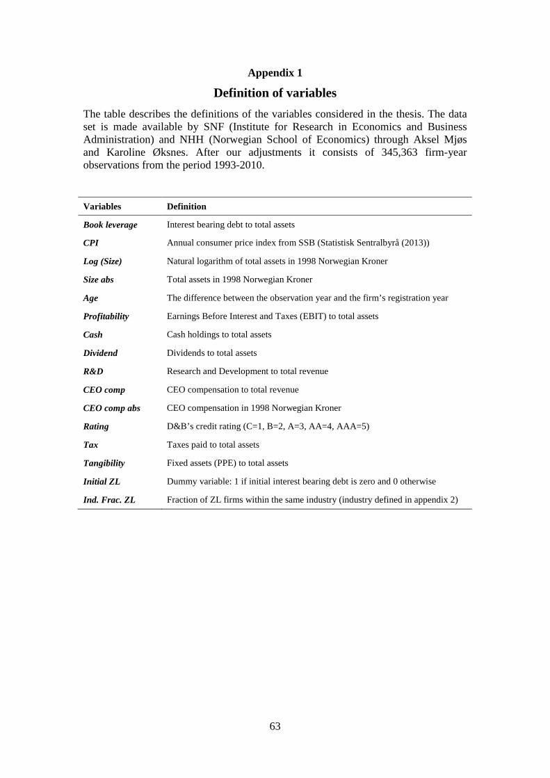
Appendix 1

Definition of variables The table describes the definitions of the variables considered in the thesis. The data set is made available by SNF (Institute for Research in Economics and Business Administration) and NHH (Norwegian School of Economics) through Aksel Mjøs and Karoline Øksnes. After our adjustments it consists of 345,363 firm-year observations from the period 1993-2010. Variables Definition

Book leverage Interest bearing debt to total assets

CPI Annual consumer price index from SSB (Statistisk Sentralbyrå (2013))

Log (Size) Natural logarithm of total assets in 1998 Norwegian Kroner

Size abs Total assets in 1998 Norwegian Kroner

Age The difference between the observation year and the firm’s registration year

Profitability Earnings Before Interest and Taxes (EBIT) to total assets

Cash Cash holdings to total assets

Dividend Dividends to total assets

R&D Research and Development to total revenue

CEO comp CEO compensation to total revenue

CEO comp abs CEO compensation in 1998 Norwegian Kroner

Rating D&B’s credit rating (C=1, B=2, A=3, AA=4, AAA=5)

Tax Taxes paid to total assets

Tangibility Fixed assets (PPE) to total assets

Initial ZL Dummy variable: 1 if initial interest bearing debt is zero and 0 otherwise

Ind. Frac. ZL Fraction of ZL firms within the same industry (industry defined in appendix 2)

63

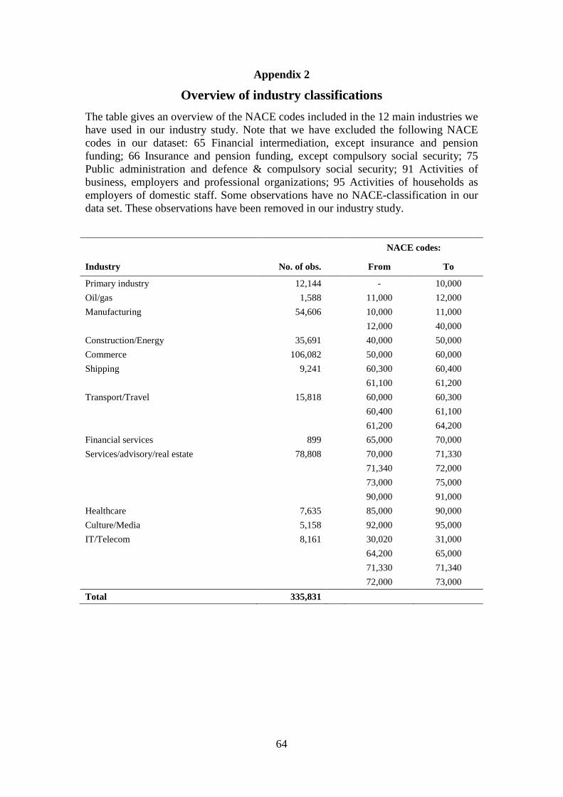
Appendix 2

Overview of industry classifications The table gives an overview of the NACE codes included in the 12 main industries we have used in our industry study. Note that we have excluded the following NACE codes in our dataset: 65 Financial intermediation, except insurance and pension funding; 66 Insurance and pension funding, except compulsory social security; 75 Public administration and defence & compulsory social security; 91 Activities of business, employers and professional organizations; 95 Activities of households as employers of domestic staff. Some observations have no NACE-classification in our data set. These observations have been removed in our industry study.

NACE codes:

Industry No. of obs. From To

Primary industry 12,144

- 10,000 Oil/gas 1,588

11,000 12,000

Manufacturing 54,606

10,000 11,000

12,000 40,000 Construction/Energy 35,691

40,000 50,000

Commerce 106,082

50,000 60,000 Shipping 9,241

60,300 60,400

61,100 61,200 Transport/Travel 15,818

60,000 60,300

60,400 61,100 61,200 64,200 Financial services 899

65,000 70,000

Services/advisory/real estate 78,808

70,000 71,330 71,340 72,000 73,000 75,000

90,000 91,000 Healthcare 7,635

85,000 90,000

Culture/Media 5,158

92,000 95,000 IT/Telecom 8,161

30,020 31,000

64,200 65,000

71,330 71,340

72,000 73,000 Total 335,831

64

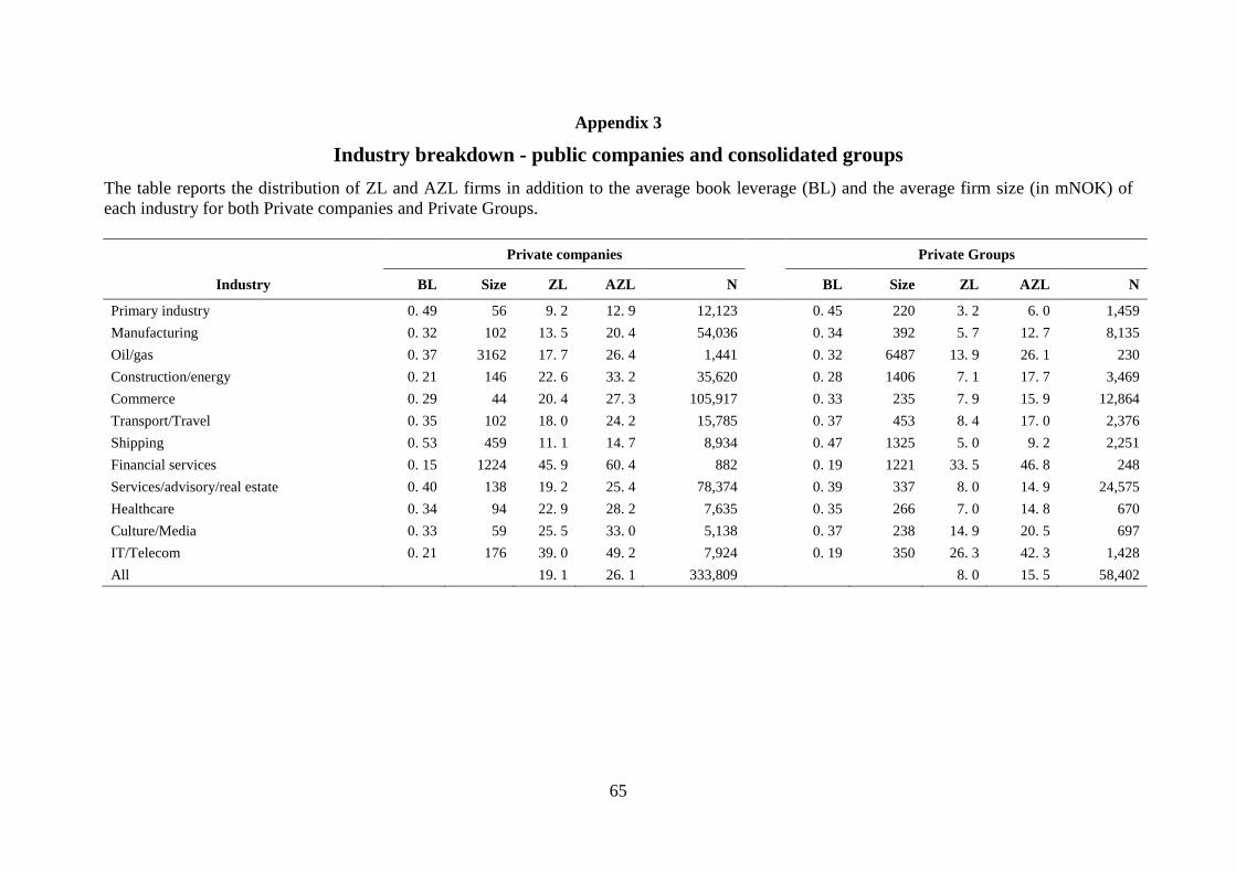
Appendix 3

Industry breakdown - public companies and consolidated groups The table reports the distribution of ZL and AZL firms in addition to the average book leverage (BL) and the average firm size (in mNOK) of each industry for both Private companies and Private Groups.

Private companies Private Groups

Industry BL Size ZL AZL N BL Size ZL AZL N

Primary industry 0. 49 56 9. 2 12. 9 12,123 0. 45 220 3. 2 6. 0 1,459 Manufacturing 0. 32 102 13. 5 20. 4 54,036 0. 34 392 5. 7 12. 7 8,135 Oil/gas 0. 37 3162 17. 7 26. 4 1,441 0. 32 6487 13. 9 26. 1 230 Construction/energy 0. 21 146 22. 6 33. 2 35,620 0. 28 1406 7. 1 17. 7 3,469 Commerce 0. 29 44 20. 4 27. 3 105,917 0. 33 235 7. 9 15. 9 12,864 Transport/Travel 0. 35 102 18. 0 24. 2 15,785 0. 37 453 8. 4 17. 0 2,376 Shipping 0. 53 459 11. 1 14. 7 8,934 0. 47 1325 5. 0 9. 2 2,251 Financial services 0. 15 1224 45. 9 60. 4 882 0. 19 1221 33. 5 46. 8 248 Services/advisory/real estate 0. 40 138 19. 2 25. 4 78,374 0. 39 337 8. 0 14. 9 24,575 Healthcare 0. 34 94 22. 9 28. 2 7,635 0. 35 266 7. 0 14. 8 670 Culture/Media 0. 33 59 25. 5 33. 0 5,138 0. 37 238 14. 9 20. 5 697 IT/Telecom 0. 21 176 39. 0 49. 2 7,924 0. 19 350 26. 3 42. 3 1,428 All 19. 1 26. 1 333,809 8. 0 15. 5 58,402

65

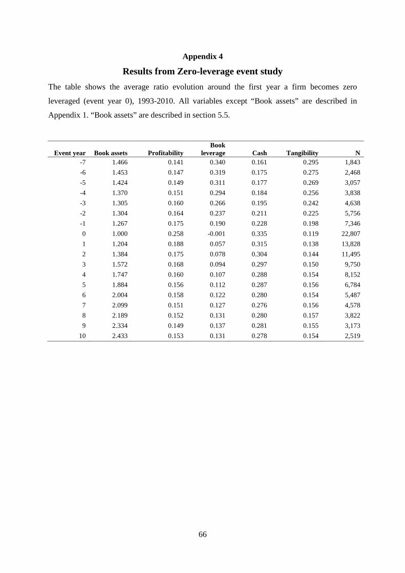
Appendix 4

Results from Zero-leverage event study The table shows the average ratio evolution around the first year a firm becomes zero

leveraged (event year 0), 1993-2010. All variables except “Book assets” are described in

Appendix 1. “Book assets” are described in section 5.5.

Event year Book assets Profitability Book

leverage Cash Tangibility N -7 1.466 0.141 0.340 0.161 0.295 1,843 -6 1.453 0.147 0.319 0.175 0.275 2,468 -5 1.424 0.149 0.311 0.177 0.269 3,057 -4 1.370 0.151 0.294 0.184 0.256 3,838 -3 1.305 0.160 0.266 0.195 0.242 4,638 -2 1.304 0.164 0.237 0.211 0.225 5,756 -1 1.267 0.175 0.190 0.228 0.198 7,346 0 1.000 0.258 -0.001 0.335 0.119 22,807 1 1.204 0.188 0.057 0.315 0.138 13,828 2 1.384 0.175 0.078 0.304 0.144 11,495 3 1.572 0.168 0.094 0.297 0.150 9,750 4 1.747 0.160 0.107 0.288 0.154 8,152 5 1.884 0.156 0.112 0.287 0.156 6,784 6 2.004 0.158 0.122 0.280 0.154 5,487 7 2.099 0.151 0.127 0.276 0.156 4,578 8 2.189 0.152 0.131 0.280 0.157 3,822 9 2.334 0.149 0.137 0.281 0.155 3,173

10 2.433 0.153 0.131 0.278 0.154 2,519

66

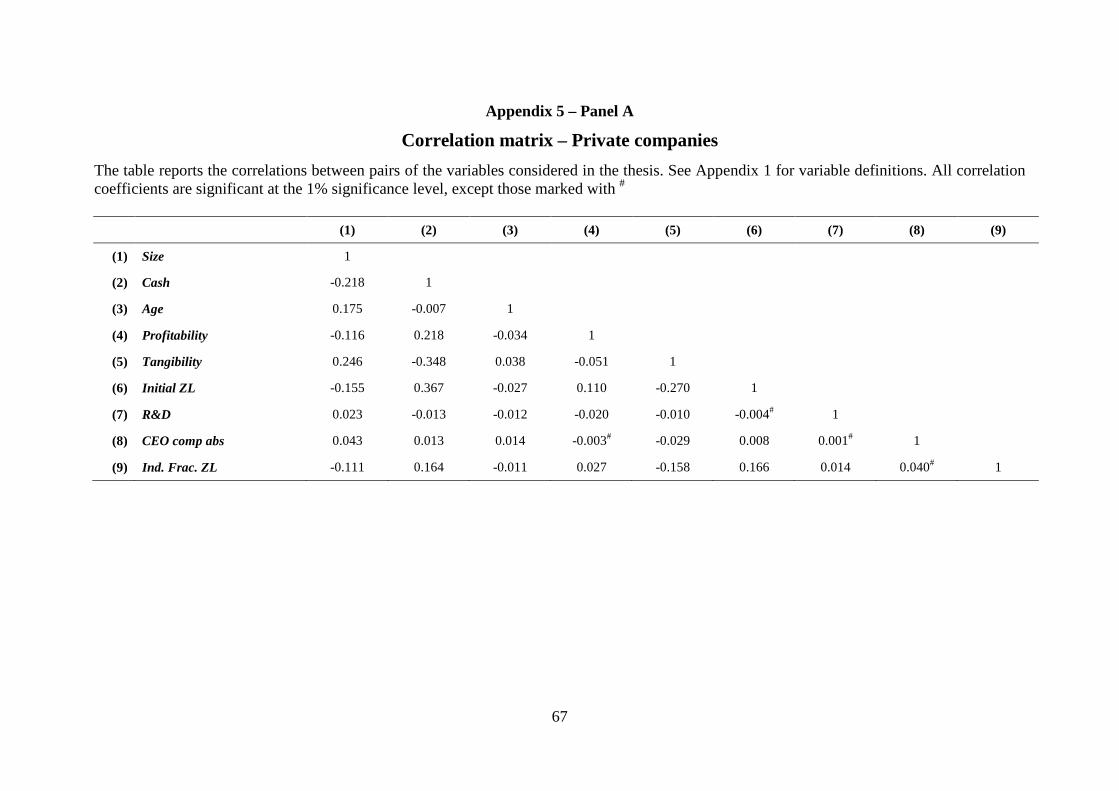
Appendix 5 – Panel A

Correlation matrix – Private companies The table reports the correlations between pairs of the variables considered in the thesis. See Appendix 1 for variable definitions. All correlation coefficients are significant at the 1% significance level, except those marked with #

(1) (2) (3) (4) (5) (6) (7) (8) (9)

(1) Size 1 (2) Cash -0.218 1 (3) Age 0.175 -0.007 1 (4) Profitability -0.116 0.218 -0.034 1 (5) Tangibility 0.246 -0.348 0.038 -0.051 1 (6) Initial ZL -0.155 0.367 -0.027 0.110 -0.270 1 (7) R&D 0.023 -0.013 -0.012 -0.020 -0.010 -0.004# 1 (8) CEO comp abs 0.043 0.013 0.014 -0.003# -0.029 0.008 0.001# 1 (9) Ind. Frac. ZL -0.111 0.164 -0.011 0.027 -0.158 0.166 0.014 0.040# 1

67

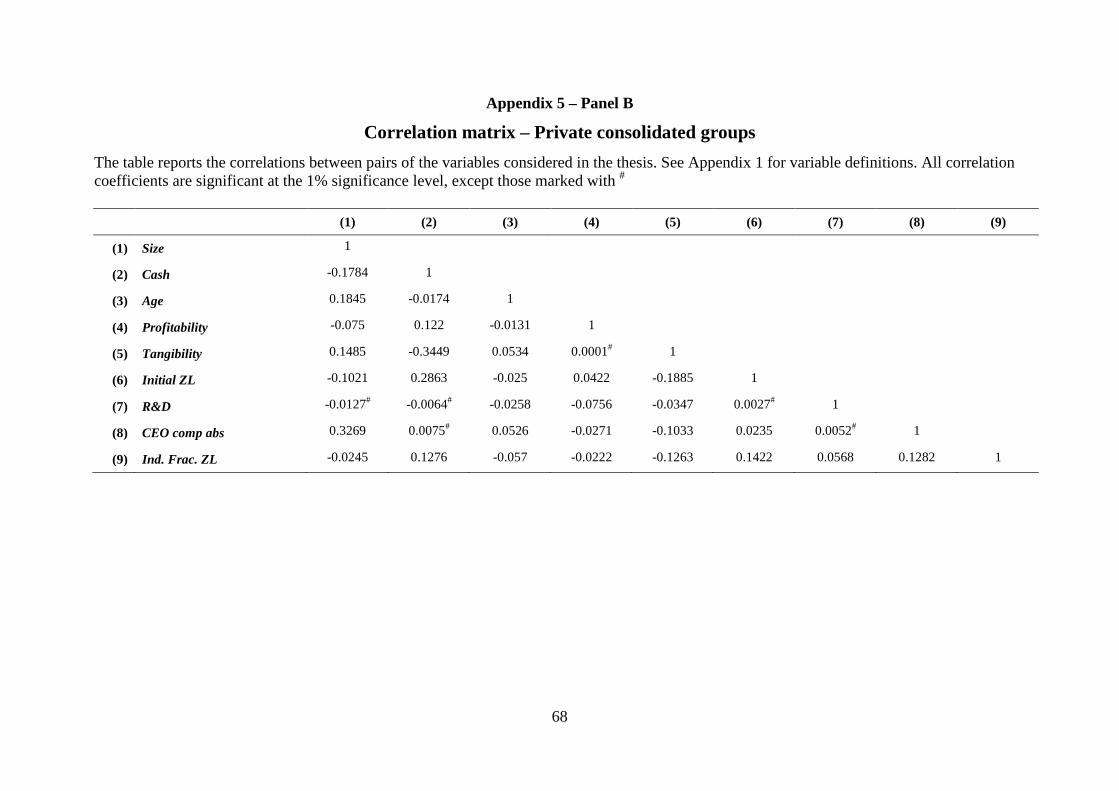
Appendix 5 – Panel B

Correlation matrix – Private consolidated groups The table reports the correlations between pairs of the variables considered in the thesis. See Appendix 1 for variable definitions. All correlation coefficients are significant at the 1% significance level, except those marked with #

(1) (2) (3) (4) (5) (6) (7) (8) (9)

(1) Size 1

(2) Cash -0.1784 1

(3) Age 0.1845 -0.0174 1

(4) Profitability -0.075 0.122 -0.0131 1

(5) Tangibility 0.1485 -0.3449 0.0534 0.0001# 1

(6) Initial ZL -0.1021 0.2863 -0.025 0.0422 -0.1885 1

(7) R&D -0.0127# -0.0064# -0.0258 -0.0756 -0.0347 0.0027# 1

(8) CEO comp abs 0.3269 0.0075# 0.0526 -0.0271 -0.1033 0.0235 0.0052# 1

(9) Ind. Frac. ZL -0.0245 0.1276 -0.057 -0.0222 -0.1263 0.1422 0.0568 0.1282 1

68

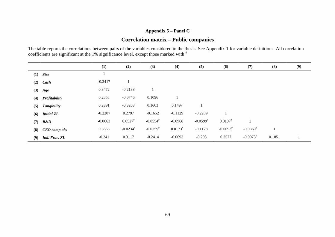
Appendix 5 – Panel C

Correlation matrix – Public companies The table reports the correlations between pairs of the variables considered in the thesis. See Appendix 1 for variable definitions. All correlation coefficients are significant at the 1% significance level, except those marked with #

(1) (2) (3) (4) (5) (6) (7) (8) (9)

(1) Size 1

(2) Cash -0.3417 1

(3) Age 0.3472 -0.2138 1

(4) Profitability 0.2353 -0.0746 0.1096 1

(5) Tangibility 0.2891 -0.3203 0.1603 0.1497 1

(6) Initial ZL -0.2207 0.2797 -0.1652 -0.1129 -0.2289 1

(7) R&D -0.0663 0.0527# -0.0554# -0.0968 -0.0599# 0.0197# 1

(8) CEO comp abs 0.3653 -0.0234# -0.0259# 0.0173# -0.1178 -0.0093# -0.0369# 1

(9) Ind. Frac. ZL -0.241 0.3117 -0.2414 -0.0693 -0.298 0.2577 -0.0073# 0.1851 1

69