BUILDING ENERGY MODEL CALIBRATION: A CASE STUDY … Library/Conferences/Specialty Conferences/2018 Building...To validate the energy model of the case study office, a number of measurements

2018 Building Performance Analysis Conference and SimBuild co-organized by ASHRAE and IBPSA-USA

Chicago, IL September 26-28, 2018

1 Submission to 2018 Building Performance Analysis Conference and SimBuild

BUILDING ENERGY MODEL CALIBRATION: A CASE STUDY USING COMPUTATIONAL FLUID DYNAMICS WITH AIR LEAKAGE TESTING AND ON-

SITE WEATHER DATA

Tat S. Fu1, Ph.D., P.E., and Edward G. Lyon1, P.E. 1Simpson, Gumpertz & Heger (SGH), Waltham, MA

ABSTRACT Whole building energy models of existing buildings are infrequently validated because of model complexity and the availability of reliable data. In this paper, the authors consider two important building energy simulation components – measured whole-building air leakage rates and on-site weather data — and study their effects on creating an accurate energy model of an existing office building in Massachusetts, USA using computational fluid dynamics (CFD) analysis. This case study shows that on-site weather data is critical in calibrating building energy models and that CFD analysis has a greater influence during a heating season compared to a cooling season in a cold climate.

INTRODUCTION Despite building energy performance simulation (BEPS) programs becoming more capable, calibrating and verifying simulation results remains challenging because of the complexity of existing buildings and resultant models, the large number of input parameters, and the availability of reliable data. This is despite the fact that the model accuracy can greatly influence designers’ and building owner’s decisions to implement building enclosure upgrades (e.g., roof replacement and insulation thickness, window replacement and glazing selection). In this paper, the authors consider two important BEPS components – measured whole building air leakage rates and on-site weather data — and study their effects on creating an accurate BEPS model of an existing office building using computational fluid dynamics (CFD) analysis. The CFD analysis helped model air infiltration (using data from air leakage test) based on external wind pressures (using data from on-site weather station). In the following sections, the authors will summarize the modeling and calibration process of an 86,400 ft2 single-story office building located in Climate Zone 5

(Massachusetts, USA). This building includes 80 mechanical zones and sub-metered electricity usage separating HVAC and plug loads. The authors installed a weather station, performed a whole building air leakage test, ran a CFD analysis of the building, and inputted these results into an EnergyPlus model to create an airflow network incorporating weather data and the measured air leakage rate. EnergyPlus, is a whole building energy simulation program that models both energy consumption and water use in buildings. The EnergyPlus model was then calibrated to reduce the difference between the simulated and sub-metered electricity usage. With the calibrated model, the authors studied the effect of using on-site weather data by simulating the model with weather data from two local airports (6 and 11 miles away from the case study building site). Finally, the authors examined the effect of incorporating an airflow network in the EnergyPlus model.

Background There are many studies on matching and calibrating BEPS models to measured data (e.g., Kaplan et al. 1990, Manke et al. 1996, Yoon et al. 2003, Reddy et al. 2007, Neto et al. 2008, Booth et al. 2013). Coakley et al. (2014) recently conducted a comprehensive review of various approaches by practitioners in developing calibrated BEPS models. These studies identified a few common modeling and calibration problems such as the lack of modeling standards, a larger number of input parameters, and uncertainty of input assumptions. In this case study, the authors focus on two key BEPS inputs: on-site weather data and air infiltration using CFD and air leakage test results. Previous efforts demonstrated the importance of available on-site weather data in model calibrations. Several successful calibration case studies relied on installing local weather stations (Royapoor and Roskilly 2014, Paliouras et al. 2015, Roberti et al. 2015). Wang et al.

© 2018 ASHRAE (www.ashrae.org) and IBPSA-USA (www.ibpsa.us). For personal use only. Additional reproduction, distribution, or transmission in either print or digital form is not permitted without ASHRAE or IBPSA-USA's prior written permission.

558


(2012) studied the uncertainties in energy consumption due to actual weather and building operational practices for an office building. The weather uncertainties/fluctuation could lead to -4% to 6% difference in predicted energy usage. Compared to calibrating BEPS models with measured local weather data, there are fewer studies using whole building air leakage testing results. Often air leakage rates are assumed in BEPS models (Parker et al. 1993, Kurnitski et al. 2009). In a comprehensive study, Monetti et al. (2015) conducted a blower door test to measure the envelope air leakage rate of a small test building (162m2 or 1,750 ft2) at the University of Liège. Along with local weather data, Monetti et al. were able to accurately calibrate their BEPS models. However, the Liège study did not include a CFD modeling of the building to better model the airflow from external wind pressures. In this paper, the authors furthered previous efforts by conducting a case study of an actual office building with local weather data, air leakage testing, and CFD analysis. The authors used this data to build a detailed airflow network in EnergyPlus to accurately simulate how weather (i.e., wind speed and direction) affect air infiltration and overall energy usage.

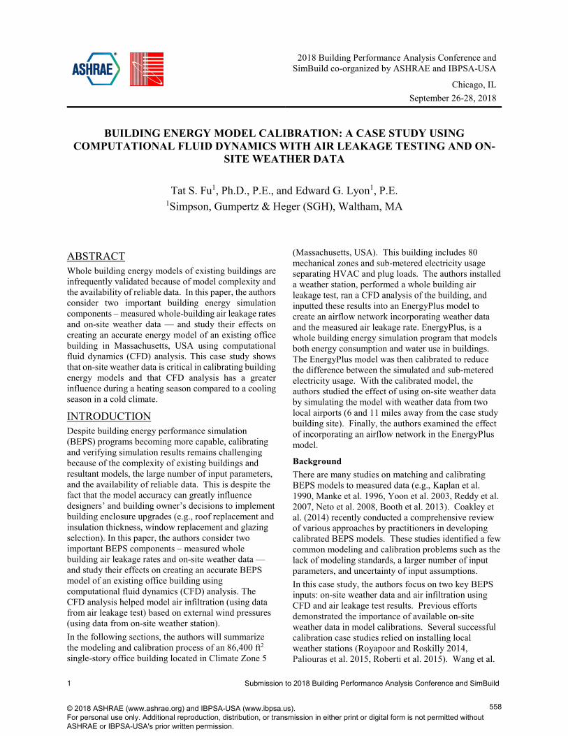
CASE STUDY BUILDING The case study building is an existing 86,400-ft2 single-story office building located in ASHRAE (American Society of Heating, Refrigerating and Air-Conditioning Engineers) Climate Zone 5 near Boston, MA. The building includes perimeter punched window openings and central clerestory windows with aluminum frames (Figures 1 and 2). 2001 renovations included new EIFS (Exterior Insulation and Finish Systems) cladding, EPDM (Ethylene Propylene Diene Monomer) roof, insulated glass units and glass curtain wall. The building’s mechanical systems include forced air heating and cooling with outdoor air ventilation.

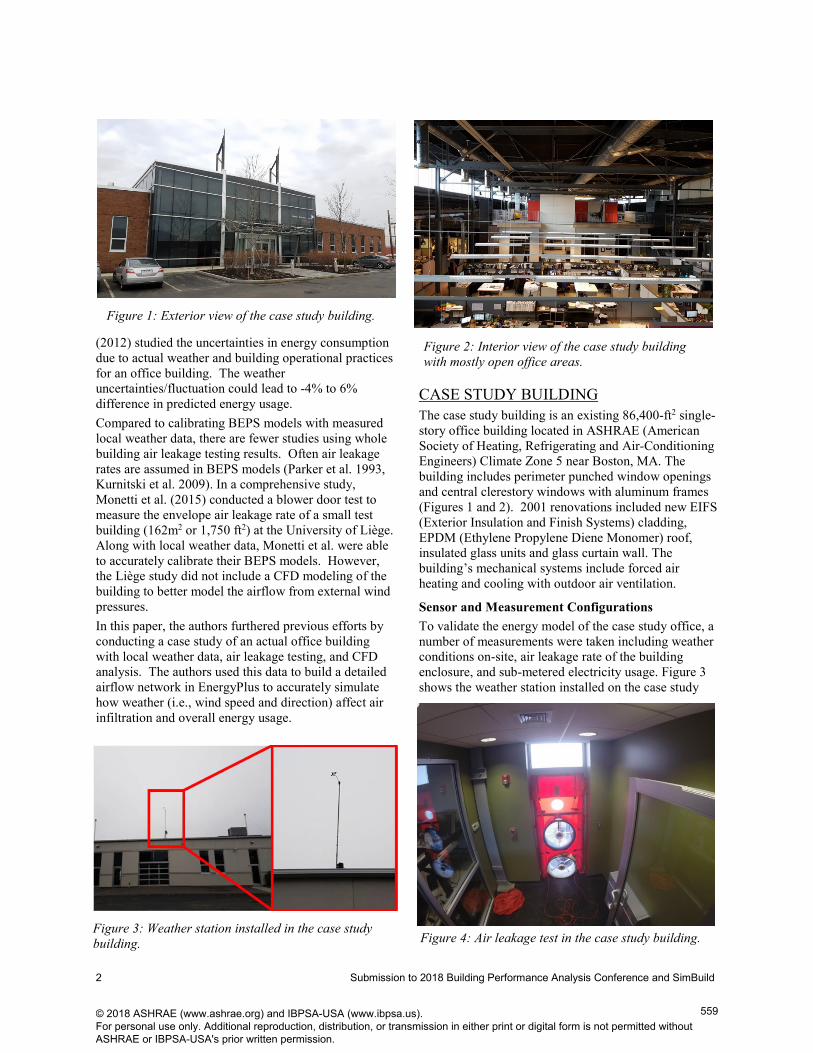
Sensor and Measurement Configurations To validate the energy model of the case study office, a number of measurements were taken including weather conditions on-site, air leakage rate of the building enclosure, and sub-metered electricity usage. Figure 3 shows the weather station installed on the case study

Figure 4: Air leakage test in the case study building. Figure 3: Weather station installed in the case study building.

Figure 1: Exterior view of the case study building.

Figure 2: Interior view of the case study building with mostly open office areas.


559


office roof. Since it was installed in 2015, the station has been recording air temperature, relative humidity, wind speed and direction, solar radiation, barometric pressure, and precipitation at 15-minute intervals. In May 2015, the authors conducted a whole building air leakage test to measure the rate of air leakage through the building enclosure (Figure 4). From the test, it was found that the primary air leakage path was through the clerestory window perimeter. The case study building office had an air leakage rate (an average of 0.26 cfm/ft2 at 75 Pa), which was below the Air Barrier Association of America guideline (0.40 cfm/ft2) and approximately equivalent to Army Corps of Engineers requirement (0.25 cfm/ft2). The air test

results included above grade building surface area only while the Army Corps standard includes slab on grade. Consequently, the case study building exceeded their requirements. The authors then coupled a CFD analysis and air leakage rate to model air infiltration and exfiltration through the building enclosure under different weather conditions (Lyon and Saldanha 2016). 0The authors also sub-metered the electrical consumption in the case study building to separate HVAC and plug loads. This information was used to calibrate the energy model such that HVAC and non-HVAC electricity usage

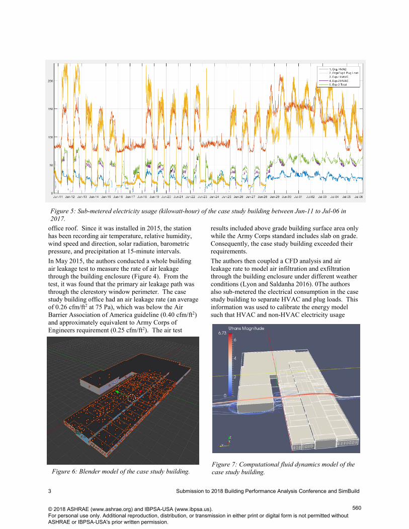
Figure 5: Sub-metered electricity usage (kilowatt-hour) of the case study building between Jun-11 to Jul-06 in 2017.

Figure 6: Blender model of the case study building. Figure 7: Computational fluid dynamics model of the case study building.


560


could be tuned separately. Figure 5 illustrates the sub-metered electricity data for a three-week period between June and July 2017.

BUILDING ENERGY MODEL The case study building includes 80 mechanical zones shown in Figure 6. The authors used Blender, an open-source 3D modeling software, to model the building geometry. ODS Studio, a plugin for Blender, was then used to convert the model geometry and airflow network into an EnergyPlus input file. In addition to creating EnergyPlus input files, the authors also used ODS Studio for virtual wind tunnel CFD analysis, shown in Figure 7. CFD results were fed into an EnergyPlus model to create an airflow network incorporating weather data and the measured air leakage rate. Table 1 summarizes several key input parameters of the EnergyPlus model. To accurately model the glazing systems, both THERM and WINDOWS by the Lawrence Berkeley National Laboratory were used to create inputs of the glazing systems in the EnergyPlus model. There are two types of double-pane glazing systems: punched windows and clerestory windows (the curtain wall entrance is similar to the clerestory windows). The exterior walls are clad with EIFS with 4 inch of expanded polystyrene (EPS) insulation. The low-slope single-ply membrane roof consists of the following components (listed from exterior to interior): EPDM membrane, wood fiberboard, 3 in. polyisocyanurate insulation, metal deck, and acoustical insulation.

Calibration Process The EnergyPlus model was calibrated to reduce the difference between the simulated and sub-metered electricity usages (Figure 8). Using the sub-metered electricity data that separated HVAC and plug loads, the authors were able to calibrate HVAC and plug loads separately. By adjusting lighting and equipment loads during the occupied and unoccupied time periods, the simulated consumption could match very closely to the sub-meter plug load data.

Calibrating according to the HVAC sub-meter data led to adjusting the heating and cooling temperature setpoints to the values shown in Table 1. The authors’ review of the monthly natural gas invoices confirmed that natural gas was not used for heating purposes during the warmer months (May to September).

One of the biggest errors in the model calibration was the occupancy on Saturdays, which is a non-business day. On Saturdays, there are usually some occupants in the office but the number of occupants varies greatly

from week to week. To estimate the number of Saturday occupants, the authors monitored the keyless entry system of the office, which records the employees who enter the building using their designated key fobs to unlock the doors. The authors reviewed Saturday entries for four months and determined that, on average, 10% of the 500 staff would occupy the building on Saturdays. After completing the abovementioned calibration, the calibrated model ended up with a CVRMSE (coefficient of variation of the root mean square error) of 5% using the calculation method published in the ASHRAE Guide 14.

RESULTS AND DISCUSSION Utilizing the calibrated model, the authors conducted several studies to examine the effect of weather station locations and using an airflow network that incorporates CFD analysis.

Weather Stations The authors used two local airports’ weather data: Bedford Hanscom Airforce Base (Hanscom) and Boston Logan Airport (Logan) to simulate the predicted

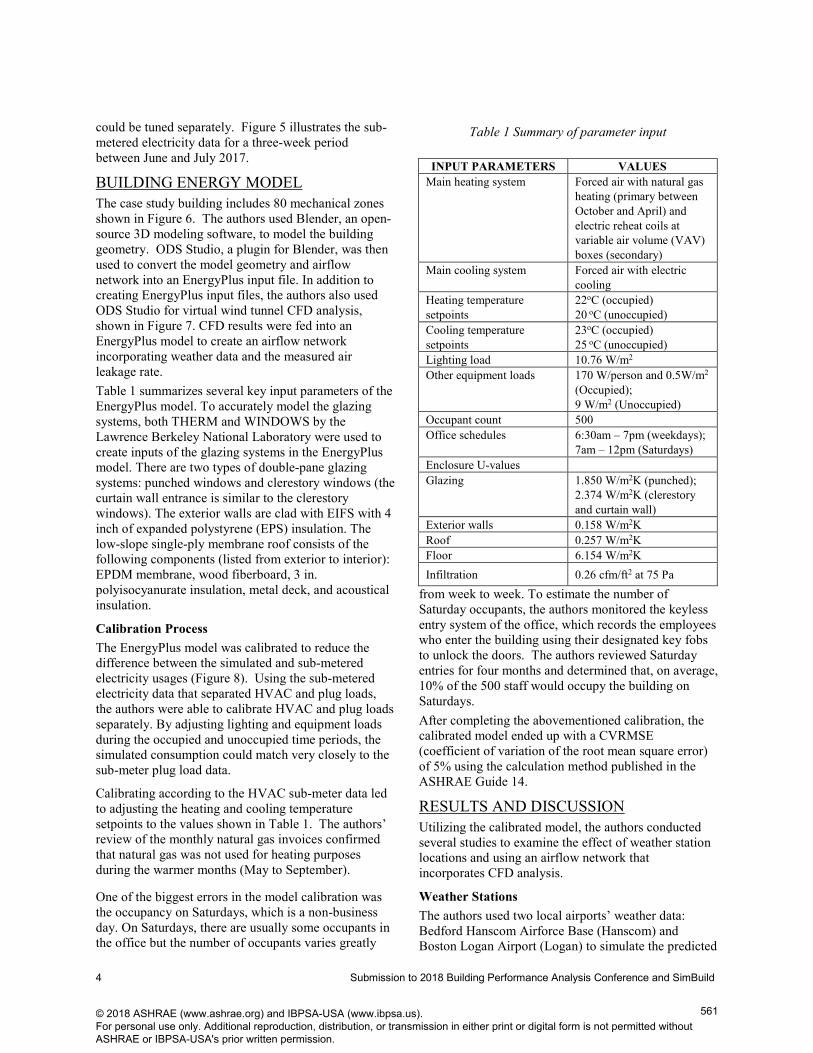
Table 1 Summary of parameter input

INPUT PARAMETERS VALUES Main heating system Forced air with natural gas

heating (primary between October and April) and electric reheat coils at variable air volume (VAV) boxes (secondary)

Main cooling system Forced air with electric cooling

Heating temperature setpoints

22oC (occupied) 20 oC (unoccupied)

Cooling temperature setpoints

23oC (occupied) 25 oC (unoccupied)

Lighting load 10.76 W/m2 Other equipment loads 170 W/person and 0.5W/m2

(Occupied); 9 W/m2 (Unoccupied)

Occupant count 500 Office schedules 6:30am – 7pm (weekdays);

7am – 12pm (Saturdays) Enclosure U-values Glazing 1.850 W/m2K (punched);

2.374 W/m2K (clerestory and curtain wall)

Exterior walls 0.158 W/m2K Roof 0.257 W/m2K Floor 6.154 W/m2K Infiltration 0.26 cfm/ft2 at 75 Pa


561


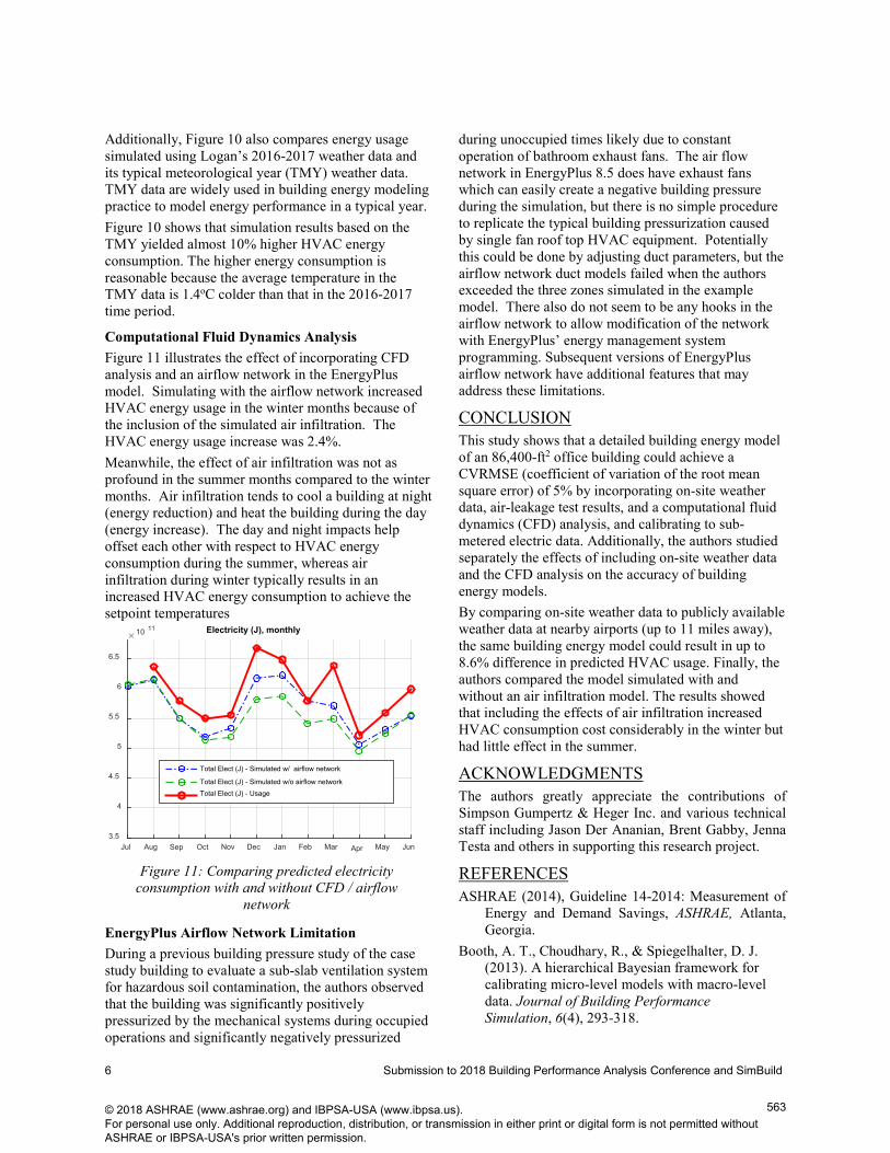
HVAC annual energy usage in the case study building. Airport weather data were served as comparisons because they are often publicly available, and it is a common practice to use nearby airport weather data when on-site weather data are not available. Despite the close proximity of the weather stations (i.e., 6.5 and 11 miles away from the case study building as shown in Figure 9), the simulated HVAC annual energy usage showed increases of 8.6% and 3.1%, respectively (Figure 10). The higher energy usages

could be contributed by slightly colder weather in Hanscom and higher wind speed (and the subsequent larger envelope air infiltration) in both the Hanscom and Logan weather station locations.

Figure 10: Predicted HVAC energy consumption using different weather stations

SGH 2016-17 BOS 2016-17 BED 2016-17 BOS-TMY0

2

4

6

8

10

12

14

0.0

3.1

8.6

12.9

HVAC annual usage as a % to baseline case

Figure 9: Weather station locations

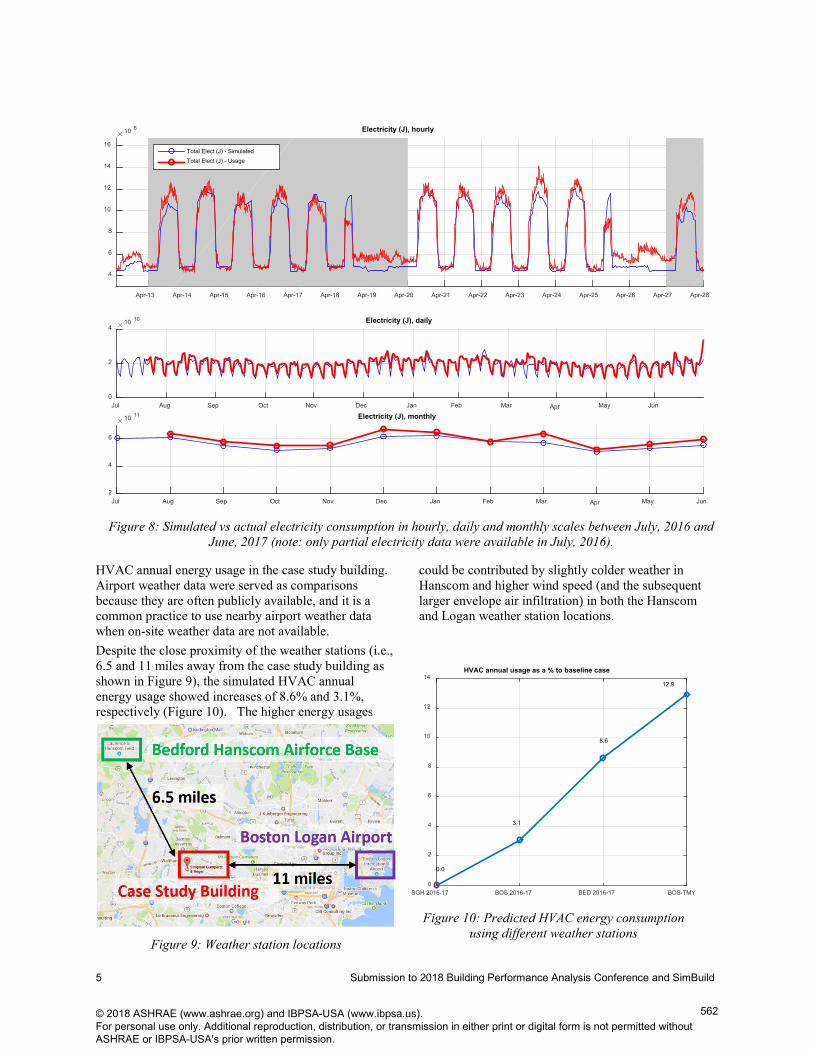
Figure 8: Simulated vs actual electricity consumption in hourly, daily and monthly scales between July, 2016 and June, 2017 (note: only partial electricity data were available in July, 2016).

Apr-13 Apr-14 Apr-15 Apr-16 Apr-17 Apr-18 Apr-19 Apr-20 Apr-21 Apr-22 Apr-23 Apr-24 Apr-25 Apr-26 Apr-27 Apr-28

10 8

4

6

8

10

12

14

16

Electricity (J), hourly

Jul Aug Sep Oct Nov Dec Jan Feb Mar Apr May Jun

10 10

0

2

4Electricity (J), daily


10 11

2

4

6

Electricity (J), monthly

Total Elect (J) - SimulatedTotal Elect (J) - Usage


562


Additionally, Figure 10 also compares energy usage simulated using Logan’s 2016-2017 weather data and its typical meteorological year (TMY) weather data. TMY data are widely used in building energy modeling practice to model energy performance in a typical year. Figure 10 shows that simulation results based on the TMY yielded almost 10% higher HVAC energy consumption. The higher energy consumption is reasonable because the average temperature in the TMY data is 1.4oC colder than that in the 2016-2017 time period.

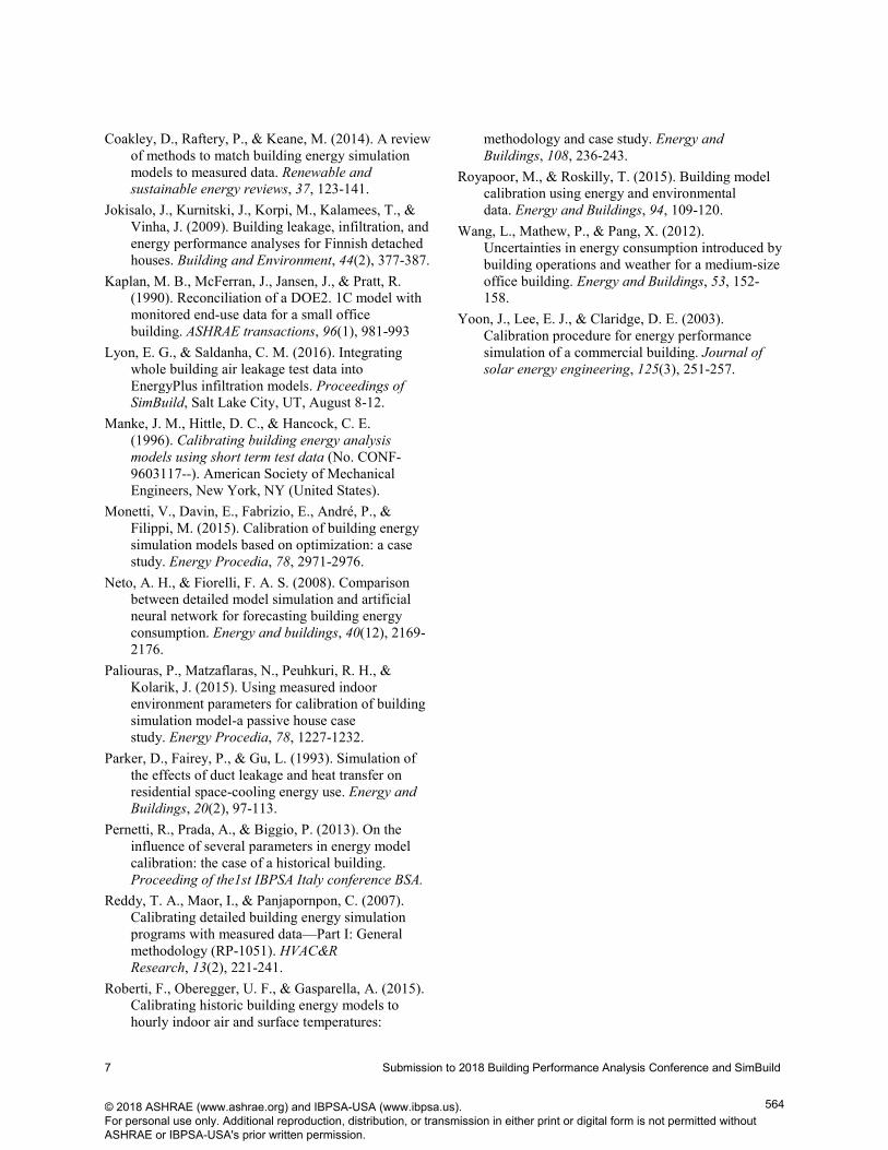
Computational Fluid Dynamics Analysis Figure 11 illustrates the effect of incorporating CFD analysis and an airflow network in the EnergyPlus model. Simulating with the airflow network increased HVAC energy usage in the winter months because of the inclusion of the simulated air infiltration. The HVAC energy usage increase was 2.4%. Meanwhile, the effect of air infiltration was not as profound in the summer months compared to the winter months. Air infiltration tends to cool a building at night (energy reduction) and heat the building during the day (energy increase). The day and night impacts help offset each other with respect to HVAC energy consumption during the summer, whereas air infiltration during winter typically results in an increased HVAC energy consumption to achieve the setpoint temperatures

EnergyPlus Airflow Network Limitation During a previous building pressure study of the case study building to evaluate a sub-slab ventilation system for hazardous soil contamination, the authors observed that the building was significantly positively pressurized by the mechanical systems during occupied operations and significantly negatively pressurized

during unoccupied times likely due to constant operation of bathroom exhaust fans. The air flow network in EnergyPlus 8.5 does have exhaust fans which can easily create a negative building pressure during the simulation, but there is no simple procedure to replicate the typical building pressurization caused by single fan roof top HVAC equipment. Potentially this could be done by adjusting duct parameters, but the airflow network duct models failed when the authors exceeded the three zones simulated in the example model. There also do not seem to be any hooks in the airflow network to allow modification of the network with EnergyPlus’ energy management system programming. Subsequent versions of EnergyPlus airflow network have additional features that may address these limitations.

CONCLUSION This study shows that a detailed building energy model of an 86,400-ft2 office building could achieve a CVRMSE (coefficient of variation of the root mean square error) of 5% by incorporating on-site weather data, air-leakage test results, and a computational fluid dynamics (CFD) analysis, and calibrating to sub-metered electric data. Additionally, the authors studied separately the effects of including on-site weather data and the CFD analysis on the accuracy of building energy models. By comparing on-site weather data to publicly available weather data at nearby airports (up to 11 miles away), the same building energy model could result in up to 8.6% difference in predicted HVAC usage. Finally, the authors compared the model simulated with and without an air infiltration model. The results showed that including the effects of air infiltration increased HVAC consumption cost considerably in the winter but had little effect in the summer.

ACKNOWLEDGMENTS The authors greatly appreciate the contributions of Simpson Gumpertz & Heger Inc. and various technical staff including Jason Der Ananian, Brent Gabby, Jenna Testa and others in supporting this research project.

REFERENCES ASHRAE (2014), Guideline 14-2014: Measurement of

Energy and Demand Savings, ASHRAE, Atlanta, Georgia.

Booth, A. T., Choudhary, R., & Spiegelhalter, D. J. (2013). A hierarchical Bayesian framework for calibrating micro-level models with macro-level data. Journal of Building Performance Simulation, 6(4), 293-318.

Figure 11: Comparing predicted electricity consumption with and without CFD / airflow

network


10 11

3.5

4

4.5

5

5.5

6

6.5

Electricity (J), monthly

Total Elect (J) - Simulated w/ airflow network

Total Elect (J) - Simulated w/o airflow networkTotal Elect (J) - Usage


563


Coakley, D., Raftery, P., & Keane, M. (2014). A review of methods to match building energy simulation models to measured data. Renewable and sustainable energy reviews, 37, 123-141.

Jokisalo, J., Kurnitski, J., Korpi, M., Kalamees, T., & Vinha, J. (2009). Building leakage, infiltration, and energy performance analyses for Finnish detached houses. Building and Environment, 44(2), 377-387.

Kaplan, M. B., McFerran, J., Jansen, J., & Pratt, R. (1990). Reconciliation of a DOE2. 1C model with monitored end-use data for a small office building. ASHRAE transactions, 96(1), 981-993

Lyon, E. G., & Saldanha, C. M. (2016). Integrating whole building air leakage test data into EnergyPlus infiltration models. Proceedings of SimBuild, Salt Lake City, UT, August 8-12.

Manke, J. M., Hittle, D. C., & Hancock, C. E. (1996). Calibrating building energy analysis models using short term test data (No. CONF-9603117--). American Society of Mechanical Engineers, New York, NY (United States).

Monetti, V., Davin, E., Fabrizio, E., André, P., & Filippi, M. (2015). Calibration of building energy simulation models based on optimization: a case study. Energy Procedia, 78, 2971-2976.

Neto, A. H., & Fiorelli, F. A. S. (2008). Comparison between detailed model simulation and artificial neural network for forecasting building energy consumption. Energy and buildings, 40(12), 2169-2176.

Paliouras, P., Matzaflaras, N., Peuhkuri, R. H., & Kolarik, J. (2015). Using measured indoor environment parameters for calibration of building simulation model-a passive house case study. Energy Procedia, 78, 1227-1232.

Parker, D., Fairey, P., & Gu, L. (1993). Simulation of the effects of duct leakage and heat transfer on residential space-cooling energy use. Energy and Buildings, 20(2), 97-113.

Pernetti, R., Prada, A., & Biggio, P. (2013). On the influence of several parameters in energy model calibration: the case of a historical building. Proceeding of the1st IBPSA Italy conference BSA.

Reddy, T. A., Maor, I., & Panjapornpon, C. (2007). Calibrating detailed building energy simulation programs with measured data—Part I: General methodology (RP-1051). HVAC&R Research, 13(2), 221-241.

Roberti, F., Oberegger, U. F., & Gasparella, A. (2015). Calibrating historic building energy models to hourly indoor air and surface temperatures:

methodology and case study. Energy and Buildings, 108, 236-243.

Royapoor, M., & Roskilly, T. (2015). Building model calibration using energy and environmental data. Energy and Buildings, 94, 109-120.

Wang, L., Mathew, P., & Pang, X. (2012). Uncertainties in energy consumption introduced by building operations and weather for a medium-size office building. Energy and Buildings, 53, 152-158.

Yoon, J., Lee, E. J., & Claridge, D. E. (2003). Calibration procedure for energy performance simulation of a commercial building. Journal of solar energy engineering, 125(3), 251-257.


564

Documents

BUILDING ENERGY MODEL CALIBRATION: A CASE STUDY … Library/Conferences/Specialty Conferences/2018 Building...To validate the energy model of the case study office, a number of measurements