Embed Size (px)
Citation preview
1ANALISIS TRIWULANAN: Perkembangan Moneter, Perbankan dan Sistem Pembayaran, Triwulan II - 2007
BULLETIN OF MONETARY ECONOMICS AND BANKING
Directorate of Economic Research and Monetary PolicyBank Indonesia
PatronPatronPatronPatronPatronBoard of Governor Bank Indonesia
Editorial BoardEditorial BoardEditorial BoardEditorial BoardEditorial BoardProf. Dr. Anwar Nasution
Prof. Dr. Miranda S. GoeltomProf. Dr. Insukindro
Prof. Dr. Iwan Jaya AzisProf. Iftekhar HasanDr. M. Syamsuddin
Dr. Perry WarjiyoDr. Halim Alamsyah
Dr. Iskandar SimorangkirDr. Solikin M. JuhroDr. Haris Munandar
Dr. Andi M. Alfian Parewangi
Editorial ChairmanEditorial ChairmanEditorial ChairmanEditorial ChairmanEditorial ChairmanDr. Perry Warjiyo
Dr. Iskandar Simorangkir
Executive DirectorExecutive DirectorExecutive DirectorExecutive DirectorExecutive DirectorDr. Andi M. Alfian Parewangi
SecretariatSecretariatSecretariatSecretariatSecretariatToto Zurianto, MBA
MS. Artiningsih, MBA
The Bulletin of Monetary Economics and Banking (BEMP) is a quarterly accreditedjournal published by Directorate of Economic Research and Monetary Policy-BankIndonesia. The views expressed in this publication are those of the author(s) anddo not necessarily reflect those of Bank Indonesia.
We invite academician and practitioners to write on this journal. Please submityour paper and send it via mail to: [email protected]. See the writing guideon the back of this book.
This journal is published quarterly; January √ April √ August √ October. The digitalversions including all back issues are available online; please visit our stable link:√http://www.bi.go.id/web/id/Publikasi/Jurnal+Ekonomi/. If you are interested to sub-scribe for printed version, please contact our distribution department: Publicationand Administration Section √ Directorate of Economy and Monetary Statistics,Bank Indonesia, Building Sjafruddin Prawiranegara, 2nd Floor - Jl. M. H. ThamrinNo.2 Central Jakarta, Indonesia, Ph. +62-21-3818202, Fax. +62-21-3802283,Email: [email protected].
BULLETIN OF MONETARY, ECONOMICSAND BANKING
Volume 14, Number 1, July 2011
QUARTERLY ANALYSIS: The Progress of Monetary, Banking and Payment System,
Quarter II - 2011
Author Team of Quarterly Report, Bank Indonesia
Persistence of Inflation in Jakarta and Its Implication on the Regional Inflation Control
Policy
Trinil Arimurti, Budi Trisnanto
Sovereign Risk Analysis of Developing Countries: Findings From Credit Default Swap
Premium Behaviour
Moch. Doddy Ariefianto, Soenartomo Soepomo
Determinant of Bank Runs In Indonesia: Bad Luck or Fundamental ?
Iskandar Simorangkir
Long-Run Money and Inflation Neutrality Test inIndonesia
Arintoko
5
51
1
31
75

1QUARTERLY ANALYSIS: The Progress of Monetary, Banking and Payment System, Quarter II, 2011
QUARTERLY ANALYSIS:The Progress of Monetary, Banking and Payment System
Quarter II - 2011
Author Team of Quarterly Report, Bank Indonesia
The Board of Governors Meeting (Rapat Dewan Gubernur/RDG) of Bank Indonesia on 12
April 2011 has decided to maintain the BI rate by 6.75%. This decision does not change the
direction of Bank Indonesia»s monetary policy which tends to be strict in an effort to control the
inflationary pressures that are still high, amid the government efforts to reduce inflationary
pressure from volatile foods group. The Board of Governors considered that the strengthening
of the rupiah so far can reduce these inflationary pressures, particularly from the rising price of
international commodities (imported inflation). In addition, to minimize the negative impact of
short-term foreign capital flows on monetary stability and financial system, the Board of
Governors also has decided to replace the one-month holding period on SBI to six-month
holding period, which shall take effect on May 13, 2011. Looking ahead, Bank Indonesia assessed
that the possibility of the BI rate level adjustment is still open to dampen the incoming inflationary
pressures. Bank Indonesia believed that the implementation of monetary and macro-prudential
policy mix, supported also by the strengthened coordination of government policy, will be able
to maintain the macroeconomic stability and bring inflation to the target, which are 5% ± 1%
in 2011 and 4.5% ± 1% in 2012.
The Board of Governors considered that the global economic recovery in the future is
better as seen from the upward adjustment of global economic growth projections by various
international agencies. This improvement of global optimism will have an impact on world
trade volume which has now also increased. This will have positive influence on the demand
for export products to help encouraging domestic economic growth. However, the process of
global economic recovery is still faced with the uncertainties related to the risk of debt crisis
that hit several countries in Europe and the potential disruption of production after the
earthquake in Japan. In addition, the rising prices of oil and global food commodity are predicted
to continue which cause inflationary pressures in many developed countries and emerging
economies, including Indonesia.
2 Bulletin of Monetary, Economics and Banking, July 2011
On the domestic side, the Board of Governors observed that Indonesia»s economic growth
is forecasted to increase by 6.0 to 6.5% in 2011 and 6.1 to 6.6% in 2012. This economic
recovery is underpinned by a more balanced source of growth in line with the improving
investment performance and the export performance that remains solid. In the second quarter
of 2011, economic growth is forecasted to grow quite high at 6.4%. The role of investment to
increase the capacity of the economy, especially through FDI, is expected to rise in line with the
demand that remains strong, both from domestic and external, and also with the improvement
in sovereign credit rating. By sector, all sectors of the economy are predicted to grow high, with
the highest growth in the sector of transport & communication, trade, hotels & restaurants,
and construction.
The performance of Indonesia»s balance of payments recorded a surplus which is estimated
to be still high enough in 2011. This surplus is derived either from the current account or from
the capital and financial transactions. Export is forecasted to grow quite high. Capital inflows,
in the form of portfolio, are predicted to remain large, while the foreign direct investment (FDI)
is expected to increase. With such development until the end of March 2011, foreign reserves
stood at 105.7 billion U.S. dollars, equivalent to 6.3 months of imports and foreign debt
payments.
The strengthening trend in rupiah continued in March 2011. In addition to being in line
with the performance of BOP, which recorded a grand surplus and foreign investors» positive
perception toward the strength of Indonesia»s economic fundamentals, the strengthening of
rupiah is also a part of Bank Indonesia»s policy response to control inflationary pressures,
particularly from the rising prices of international commodity (imported inflation). Until the end
of March 2011 the rupiah was strengthened by 3.47% (ptp) to Rp8.708 per U.S. dollar. This
appreciation to Rupiah has not so far affected the competitiveness of Indonesia in terms of the
exchange rate, among others, reflected in the performance of Indonesia»s non-oil exports which
continue to show a relatively high improvement.
In regard to price, although the inflation has shown a declining trend, the risk of future
inflation pressures is expected to remain quite high. CPI inflation in March 2011 reached 6.65%
(yoy) or deflation of 0.32% (mtm) in line with inflation correction in alimentation products.
Although it is still relatively high, the inflationary pressure from the volatile foods group showed
a declining trend in line with the Government measures to strengthen the national food.
Meanwhile the moderate inflation of administered prices is associated with the minimum price
adjustment policies by the Government. However, the core inflation showed an increasing
trend, which was recorded at 4.45% (yoy) or 0.25% (mtm) in March 2011, as the propagated
impacts of the high prices of food and the rising inflation expectations. Looking ahead, the risk

3QUARTERLY ANALYSIS: The Progress of Monetary, Banking and Payment System, Quarter II, 2011
of inflationary pressures is expected to remain relatively high, influenced by the rising prices of
international commodity, the high domestic demand, and the high inflation expectations. Bank
Indonesia will continue to be alert to the risk of inflationary pressures and strengthen the
mixture of monetary and macro-prudential policy to control the inflation targets.
The stability of financial system is maintained along with the continuing improvement of
the intermediation function of banks and the banking liquidity which is in control. The banking
industry is under a stable condition characterized by the sustained capital and liquidity as
reflected in the high capital adequacy ratio (CAR) at the level of 18% and the ratio of
nonperforming loans (NPL) which is maintained fewer than 5% gross. The banking
intermediation is also getting better reflected in the rising credit growth, which in March 2011
reached 25.1% (yoy), supported by the growth in all types of loans including loans to Small
Medium Enterprises (SMEs).

4 Bulletin of Monetary, Economics and Banking, July 2011
This page is intentionally left blank
5Persistence of Inflation in Jakarta and Its Implication on the Regional Inflation Control Policy
PERSISTENCE OF INFLATION IN JAKARTA AND ITS IMPLICATIONON THE REGIONAL INFLATION CONTROL POLICY
Trinil Arimurti, Budi Trisnanto 1
The main objective of this study is to measure the persistence of inflation level in Jakarta. In addition,
this study intends to find out the source of inflation persistence and its implication to regional inflation
control. The analysis of the regional inflation behavior developed in this paper is explored to commodities
level. The empirical result indicates that the level of inflation persistence in Jakarta is relatively high,
stemmed from high level of inflation persistence for most of commodities that construct inflation. Using
the estimation results of the hybrid NKPC model, it shows that high inflation persistence in Jakarta mainly
caused by inflation expectation, which is a combination of forward and backward looking. In this regards,
it requires efforts gradually transform the behavior of inflation expectation to be more forward looking.
Keywords: inflation peristence, expectation, NKPC.
JEL Classification:E31, R10
1 The views on this paper are solely of the authhors and not necessaily reflect the views of Bank Indonesia. We thank to Yoni Depari,Sugiharso Safuan and researchers on Beureau of Economc Research and Beureau of Monetary Policy, DKM, Bank Indonesia;[email protected], [email protected].
Abstract
6 Bulletin of Monetary, Economics and Banking, July 2011
I. INTRODUCTION
According to the constitution No. 13, 1968 about Bank of Indonesia (Bank Indonesia)as
finally amended with law No. 4, 2003, the duty of Bank of Indonesia is to achieve and maintain
the stability of Rupiah value toward good and service or inflation stability.Therefore, the monetary
policy is directed to achieve and maintain the inflation in the low and stable rate. In this context,
the response of monetary policy is not only determined by the inflation rate that wants to be
achieved but is also determined by the inflation behavior itself. That will determine the amount
and timing of the response of monetary policy that needs to be applied in order to reach the
inflation desired. In the side of inflation rate that wants to be achieved, the monetary policy is
directed to achieve the inflation target which is stipulated decreasing gradually to the rate that
supports the perpetual economy growth. According to the law meant, the inflation target is
stipulated by the government after coordinating with Bank of Indonesia which is purposed to
increase the credibility of monetary policy. The assessment about the inflation behavior is related
to the inflation persistence or the speed of inflation rate back to its equilibrium rate following
the shock.
Some researchers have been conducted to see the inflation persistence in Indonesia. The
result of Yanuarty study (2007) and Alamsyah (2008), for example, is to conclude that the
degree of inflation persistence in Indonesia was generally high however tended to decrease in
the crisis aftermath period. While Harmanta (2009) stated that the backward lookinginflation
persistence in the era of ITF decreased, and for theforward lookingexperienced an increase.
Nevertheless, the study needs to be supported by the regional study, in term of looking more in
regional level. It is also motivated by the understanding that the national inflation is formed
from regional inflation. More specifically, the study of inflation persistence in region by considering
that each has inflation characteristic that implicates to the inflation controlling policy though
generally inflation pressure in region mostly related to the shock in supply
The implementation of Inflation Targeting Framework (ITF) in 2005 became the milestone
of the change of monetary policy frame done after the economic crisis in Indonesia. Principally
the monetary policy frame is in order to adopt the more credible policy frame that accomplish
to the use of interest rateas operational target and anticipative policy. ITF is hoped able to
change backward looking expectationthat becomes the source of the high inflation intact, to
becomeforward looking expectation. So that, it is hoped that ITF can push the decrease of
inflation persistence.
Next, the persistence inflation needs to be supported by analysis about the cause of
inflation persistence. As understood in CPI inflation component that its price is influenced by
7Persistence of Inflation in Jakarta and Its Implication on the Regional Inflation Control Policy
government policy in the field of price and administered prices. The price in this commodity
tends to be flat and changes when there is a government policy. Besides that, there is component
that its price is influenced by supply shocksor is seasonally. For that, assessment is needed to
see the fundamental factors more detail. This is purposed so that the response of monetary
policy can be carried out more precise regarding monetary policy is for demand management.
In other words, the response of monetary policy cannot be overdone if the source of inflation
pressure from the non √ fundamental factor.
The study of the phenomenon of the inflation persistence that becomes very important
to be done in order to support formulating effective monetary policy. This thing because
the affectivity of monetary policy can support the perpetual economy growthin order to
raise the society prosperity. The high inflation will give negative impact to the economy.
Purchasing powerof society will decrease and world business will be covered by the high of
uncertainty. The implication from the inflation persistence will also be felt in the level of
region so that it needs to be looked after by local government to be able actively act in
controlling inflation.
The study is finally needed to formulate the strategy of inflation control. The source of
inflation pressure makes the inflation persistence needs to be analyzed more edge so that
can be differentiate the fundamental form the temporary source of inflation pressure. The
monetary policy cannot be fully used to respond the inflation pressure from the side of
supply.Sectoral and regional policies are needed to decrease the inflation pressure from non-
fundamental factors. There are some studies of inflation persistence that has previously been
done in Indonesia that are more focused on the national scale or range. National inflation
constitutes theweighted averagefrom inflation in the region in Indonesia, therefore it needs
to study about the behavior of inflation in the region level,including to measure and search
for its cause, and also to know its implication toward the control of the region inflation with
the focus on Jakarta.
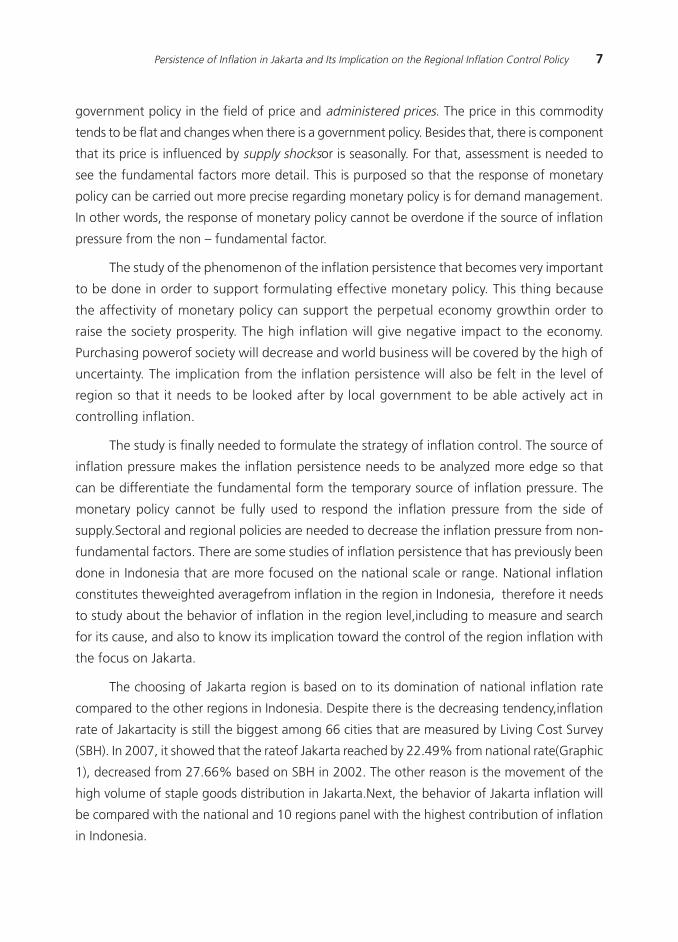
The choosing of Jakarta region is based on to its domination of national inflation rate
compared to the other regions in Indonesia. Despite there is the decreasing tendency,inflation
rate of Jakartacity is still the biggest among 66 cities that are measured by Living Cost Survey
(SBH). In 2007, it showed that the rateof Jakarta reached by 22.49% from national rate(Graphic
1), decreased from 27.66% based on SBH in 2002. The other reason is the movement of the
high volume of staple goods distribution in Jakarta.Next, the behavior of Jakarta inflation will
be compared with the national and 10 regions panel with the highest contribution of inflation
in Indonesia.
8 Bulletin of Monetary, Economics and Banking, July 2011
To answer the research objectives, the scoop of study span which are the period of January
2000 to May 2008 (Jakarta) and January 2000 to December 2009 (national). This relates to the
availability of the data from BPS until the commodity level.
Figure 1.Inflation Rateof the city based on SBH 2007
2. THEORY
The inflation persistence according to Marques (2005) is defined by the speed of inflation
rate to move back to its equilibrium spot after emergence of the shock. The high speed shows
that the low inflation persistence rate and in the way around the high inflation persistence rate
that is shown by the time used by inflation rate to move back to its equilibrium spot. The
almost same definition is also stated by Willis (2003) who defines the inflation persistence by
the time needed by the inflation to move back to its baseline after the shock. While, the
alternative definition which is more various is stated by Batini (2002) who discussed three types
of inflation persistence, which are (i) ≈positive serial correlation in inflation∆; (ii) ≈lags between
systematic monetary policy actions and their (peak) effect on inflation∆; (iii) ≈lagged responses
of inflation to non-systematic policy actions∆.
Combined 56Other Cities
47.23
Jakarta22.49
Surabaya6.47
Bandung5.38
Medan4.67
Semarang3.48
Palembang2.96
Makasar2.56
Denpasar1.53
Banjarmasin1.54
Padang1.69
Source: BPS-Statistics Indonesia, processed
9Persistence of Inflation in Jakarta and Its Implication on the Regional Inflation Control Policy
The study about inflation persistence is important to increase the ability of inflation forecast,
retrieve the clarity of dynamic effect fromexogenous price shocks, gives information/direction
and fix the monetary policy, and in order to value whether the other monetary policy regime
will produce the different persistence, Stock (2004).
2.1 The Measurement of Inflation Persistence
In order to measure the inflation persistence rate, there are two approaches that can be
used,which are the univariate approach and multivariate model approach. The univariate
approach is only more stress to the time series data aspect,while the multivariate approach
also cover additional information such as real output and central bank interest rate (Dossche
and Everaert, 2005). From some studies that have been carried out, the univariate approach
by using autoregressive (AR) time series model constitutes the most common in empiric
research.
Some scalar measurement methods (univariate)that can be used to calculate the inflation
persistence such as (i) the sum of the autoregressive(AR) coefficients; (iii) the largest
autoregressive root; (iv) the half-life (Marques, 2005). With AR model, the inflation persistence
rate is measured from the range of its lag variable. Meanwhile LAR (the largestautoregressive
root) is generally explained by Levin and Piger (2004). In this method, inflation persistence is
acquired by finding the biggest square root, the equation of 1
0
KK K j
j
j
. While
thehalf-life method is adopted especially for evaluating deviation persistence frompurchasing
power parity equilibrium (Marques 2004). As described by Andrews and Chen (1994), the
half-life formula is T
n1 , where n is the amount of some inflations above 0.5 when the
big disturbance occurred as much as 1 unit and T is the amount of observation period.
Despite there are some concepts of different inflation persistence period measurement rate,
the estimation result acquired is not far different generally. (Clark, 2003).
The research focus in the inflation process enables the use of univariate model in this
paper. However, univariate model cannot be separated from some limitations; one of them is
that this model cannot identify the cause source of the observed persistenceof inflationso that
there is the probability of inflation process potential trigger to be ignored.
Marques (2004) stated that the AR model is a good inflation persistence measurer, and is
also directly related to the coefficient of mean reversion as the alternative of inflation persistence
rate measurement. The ARformula AR with order of p can be describedas follows:
10 Bulletin of Monetary, Economics and Banking, July 2011
From the result of the equation estimation, the inflation persistence rate is calculated by
adding AR coefficient, 1
K
j
j
.
The way to calculate the coefficient is the best persistence scalar measurement way
according to Andrews and Chen (1994). Inflation persistence is high if today inflation rate is
influenced by the value of its lag, so that the coefficient is close to 1. In this case, the inflation
can be said closed to the unit root process.
To retrieve the result of estimation, in every inflation series needs to be determined the
amount of proper lag variable dependent. In its determination, Akaike Information Criterion
(AIC) or Schwarz» Bayesian Information Criterion (SBIC) can be used.As stated by Levin and
Piger (2004), in measuring the persistence by using AR model, the equivalent equation as
follows needs also to be considered:
Where the dynamic parameter φj is a simple transformation from AR coefficient from the
equation (1) constitutes simple transformation from AR coefficient from equation (1).
Specifically, persistence concept is much related to the Impulse Response Function (IRF)
from the process of AR (ρ). Marques (2004) described the weakness and the strength of each
(1)
: Monthly inflation rateat the time of t
: The constant from the result of estimation process as control toward inflation Average
: The amount of AR Coefficient
: Random error term or residual from equation regression above
(2)
t
1
K
j
j
t
11Persistence of Inflation in Jakarta and Its Implication on the Regional Inflation Control Policy
persistence measurement methods. The Cumulative Impulse Response Function (CIRF) concept
which is formulated as
1
1CIRF describes the monotonic correlation between CIRF and
the AR coefficient (ρ), so that the calculation is very dependent on the AR coefficient. The other
weakness of CIRF and ρ in measuring the inflation persistence is if there are 2 (two) of data
series, and both of the method cannot tell the different between the series that was highly
increased and then followed by the gradual decrease with the series that the increase was low
and then followed by the low high decrease in its IRF. Separated fromthe limitation that becomes
the weakness of univariate method, this scalar measurement methodmust be seen as the method
for estimating the inflation average speed to move back to its equilibrium after the emergence
of the shock.This scalar is considered more effective if the speed of inflation series convergence
is more uniformed.
Some critics toward the half-lifemethod in inflation persistence rate calculation have
been also explained in the previous research. If IRF is oscillating, this method will produce too
low inflation process persistence. Besides, if the inflation process is very persistent, the output
ofthe half-lifeis very high so it will be difficult to differentiate the change of persistence as the
time goes by. However this method is usually preferred because more understanding for its
measurement in time unit. Because of the limitation, some writers do thehalf-lifecalculation
directly from IRF. Meanwhile the critic towards thelargest autoregressive roothas ever been
stated by (2004). The persistence measurement by using this method is considered not good
since its function depends on the other root, not only from the biggest root. However the
advantage of this method is the easiness in calculating asymptotically valid confidence intervals
for its estimation result.
The calculation result of inflation persistence degree by using AR model estimated by
using OLS can be compared with the bootstrap estimation result. This is also useful to
anticipate of the probability of invalid measurement if the persistence degree closes to the
number of 1, so that the robustness check is important to be carried out. This procedure
has been used in some previous research, such as: O»Reilly and Whelan (2004) and Alamsyah
(2008).
In order to complete the observation toward inflation behavior change, rolling regression
method can be used to see whether the inflation process is changing as the time goes by, by
seeing the evolution from the AR coefficient. This method has been done also in some previous
research such as:Pivetta & Reis (2006), Debelle and Wilkinson (2002), O»Reilly and Whelan
(2004) and Alamsyah (2008). It is generally can be summarized that the estimation result of
12 Bulletin of Monetary, Economics and Banking, July 2011
inflation persistence degree by using the method showed the change of inflation process in
countries that became sample of object occurred. Nevertheless, this method has also the
weakness because not accurately showed the change of inflation persistence rate, so that the
factors influences such as monetary policy cannot be caught clearly.
In doing analysis toward inflation persistence degree, it is also need to be considered the
existence of structural breaks. Some literatures stated that the estimation of inflation persistence
rate will be exaggeratedif the existence of the inflation average value of structural break is not
calculated. Some techniques such as Andrew and Quandt test or Chow test can be carried out
to do the test toward the existence of structural break.
In order to measure of how long does the inflation take to absorb 50% of shockoccurred
before moving back to its average value, formula can be used (Gujarati, 2003) with simple
formula
1
h . Where h is the time needed by inflation to absorb the 50% of shock
occurred before moving back to its average value and ρ is the estimation result of inflation
persistence degree.
Some studies related to the inflation persistence have been done in Indonesia, such as by
Alamsyah (2008), Yanuarti (2007), Bank Indonesia inflation team (2006). Whole the research
were more stressed on the national inflation persistence and limited to general inflation
persistence and commodity group. Generally it is found that the inflation persistence degree in
Indonesia is relatively high in the observation period, though there is decreasing tendency in
the crisis aftermath period in 1997/1998. Nevertheless, there has not been a study about the
inflation persistence in regional level and covers until commodity level.
The study that has been done by Alamsyah (2008) is for seeing the inflation behavior
change in Indonesia at the time of before and after crisis, and also for seeing the cause sourceof
inflation persistence especially from the micro businessmen approached by using NKPC hybrid
model. By using univariate approach which is the sum of autoregressive coefficient (AR (1)) it is
found that the persistence degree in Indonesia is relatively high at the observation period of
1985-2007. Nevertheless, the persistence degree tends to be decreasing at the time of after
economic crisis.It is also founded that the inflation in Indonesia constitutes the combination of
backward and forward lookingbehavior. Therefore, the effort to stabilize the inflation
expectationto the target set by central bank, needs to control the inflation and increase the
monetary policy credibility in Indonesia.
Meanwhile, the study by Yanuarti (2007) was purposed to measure the inflation persistence
degree in Indonesia and also to research whether there is the change of inflation persistence
13Persistence of Inflation in Jakarta and Its Implication on the Regional Inflation Control Policy
degree change in span of 1990-2006. By using gull sample, it is found that the inflation
persistence degree in Indonesia is very high; however tends to decrease at the time of after
crisis. Thesefindings are in line with Alamsyah findings (2008).
2.2 The Cause of Inflation Persistence
Inflation pressure source can be seen through the equation of New Keynesian Philips
Curve (NKPC), where the cause of inflation persistence can be seen by the inflation forward
looking) and (backward looking)behavior. This approach is the innovation of the inflation initial
model that describes the inflation dynamic as written in NKPC:
Next, according to Gali and Gertler (1999), beside forward looking oriented, inflation has
also backward lookingbehavior both of the behaviors described from the NKPC Hybrid model
that catch the inflation persistence characteristic.
The inflation structural equation that is usually called as New Keynesian Phillips Curvehybrid
consisted in this equation below (Angeloni et. al, 2004):
Where πt is inflation at the time of t; E
t (π
t +1) is the inflation expectation at the time of t+1
with informal condition at the time of t, µt is output gap and ξ
t is exogenous shock
substance.
By seeing the right side of the equation, it can be estimated that the four of inflation
sources : (i) extrinsic persistence that relates to the persistence of marginal cost or output gap.;
(ii) intrinsic persistence that relates to the inflation dependency toward the previous period
inflation (backward looking expectation); (iii) expectations-based persistence that relates to the
inflation expectation form that is based on to the forward looking; (iv) error term persistence
because of the inflation shock occurred.
1 tttt Ey
14 Bulletin of Monetary, Economics and Banking, July 2011
III. METHODOLOGY
3.1 Estimation Technique
Inflation persistence estimation is done by seeing univariate autoregressive (AR) time
series model process as Marques (2004) stated since the AR model is the measurer of good
inflation persistenceand also directly related to the mean reversion as alternative of inflation
persistence rate measurement. AR formula with the order p can be broken down as follows:
(3)
: Monthly inflation rate at the time of t
: The constant of estimation result, as control of average inflation
: The total of AR coefficient
: Random error term or residual from equation regression above
The inflation persistence rate is calculated by adding AR coefficient .
The inflation persistence can be said high if today inflation rate is very influenced by its lag
persistence, so that the coefficient is close to 1.in this case, inflation can be said close to
the unit root process.
For, estimation, the determination of the amount of dependent variable lagwhich is
according to theAkaike Information Criterion (AIC) and or Schwarz» Bayesian Information
Criterion (SBIC). In order to see the result of robustness obtained, and also bootstrap and
rolling regression procedure is conducted. Structural break test is carried out by applying the
technic such as Quandt (1960) and Chow test to do the test toward known and unknown
break to measure of how long does the inflation take to absorb 50% of shock that is occurred
before moving to its average value, the formula is:
In this paper, the cause of inflation persistence can be seen based on the inflation behavior
forward lookingand backward looking of the inflation behavior as follows:
t
1
K
j
j
t
15Persistence of Inflation in Jakarta and Its Implication on the Regional Inflation Control Policy
Where πt is the inflation at the time of t; E
t (π
t +1) is an inflation expectation at the time of t+1
with information condition at the time of t, µt is the output gap and ξ
t is a exogenous shock
substance. The significant variable and has big coefficient is the variable that becomes the main
source of inflation pressure. Embarking from the analysis about the source of the inflation
pressure, and in order to see the inflation persistence source, more analysis is done.
In the analysis of the source of inflation persistence, the inflation is only focused on o the
5 commodities that has the highest of inflation persistence degree. The five commodities are
the most important commodities in controlling inflation. In order to analyze the source of
inflation persistence,anecdotal informationandanalysis are used and also the study that has
been done related to the commodities. The information collected such as about the market
structure and the commodity inflation characteristic.
3.2 Data
The data that will be used in this inflation persistence analysis are:
1. Monthly inflation (year-on-year), measured by using Consumer Price Index of the total of all
city in Indonesia (National inflation) and IHK of Jakarta city, also IHK 9 of other regions that
have the biggest rate toward national inflation. While the date used the year base 2002.
The IHK can be explained in detail in to 7 (seven) commodity groups : (i) Foodstuff, (ii) Food,
Baverages and Tobaccos, (iii) Estate, (iv) Clothes, (v) Health, (vi) Education, Recreation and
Sports, and (vii)Transportation and Communication.The sample span was started since January
2000 - May 2008 (December 2009 for national). The source of CPI data is retrieved from the
Statistic Center Bureau and International Financial Statistics (IFS).
2. The annual inflation target(source: Bank Indonesia)
The use of the year on year inflation data especially is because some reasons as stated by
Babecky (2008) as follows:
1. The use of month-to-month (m-t-m) inflation data or quarter-to-quarter (q-t-q) is very related
to the seasonal factor so that it is worried that it does not represent the real inflation
persistence
2. The both of inflation size m-t-m and q-t-q size are not monitored by certain economic
agent.
16 Bulletin of Monetary, Economics and Banking, July 2011
3. Central bank in determining the inflation target is more based on the annual inflation change
(y-o-y).
4. RESULT AND ANALYSIS
4.1 The development of Jakarta Inflation
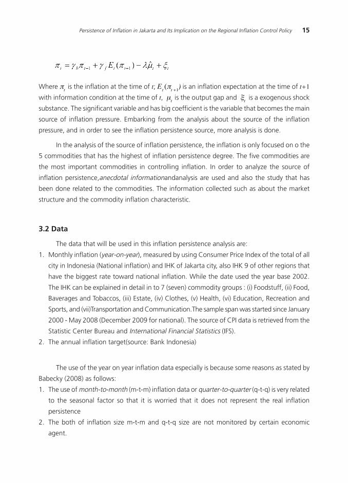
Jakarta Inflation has the almost same pattern with the national inflation. In a span of the
last 25 years, the average of Jakarta inflation rate has not been changing significantly. Either in
the before and after economic crisis period occurred in1997/1998,the average of inflation tend
to be staying at 8% (outside crisis period).While, compared with the region countries such as
Malaysia, Thailand and Philippines at that period, Indonesia inflation is relatively high (Alamsyah,
2008). The tendency of the resistance inflation rate in the high level needs to further observationin
order to determine the right pace in controlling it.
Figure 2. The development of National Inflation andJakarta and National
The high tendency in Jakarta can be still seen after applying the ITF in Indonesia. Formally,
ITF began being applied inJuly 2005 by setting inflation target periodically and transparently.
Figure 2 describes that the inflation realization either in Jakarta of National d not still sometimes
reach the target applied. This thing describes of the lateness of proses of inflation decline in
Indonesia.
-10
0
10
20
30
40
50
60
70
80
90Jakarta
NationalAverage of Jakarta Inflation
Average of National Inflation
Jan1986
Jan1988
Jan1990
Jan1992
Jan1994
Jan1996
Jan1998
Jan2000
Jan2002
Jan2004
Jan2006
Jan2008
Source: BPS-Statistics Indonesia, processed
17Persistence of Inflation in Jakarta and Its Implication on the Regional Inflation Control Policy
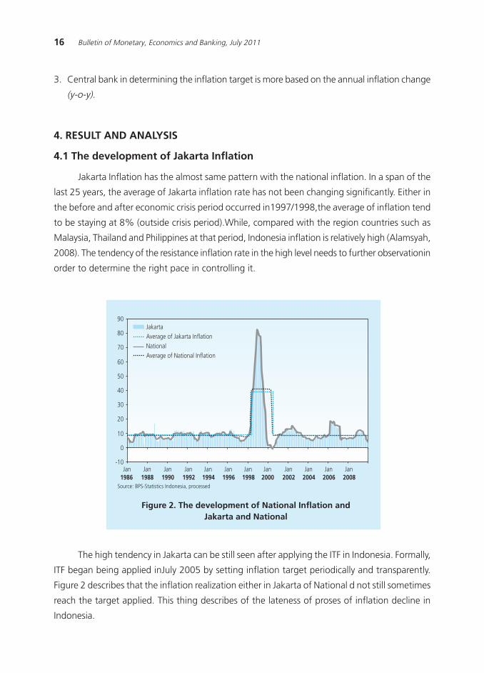
The lowest rate of year by yearinflation until 2008 that could be reached was still above
5%. If it is compared with the inflation average of the country that adopts ITF, the inflation rate
in Indonesia is still classified as high.
Figure 3.Target and inflation Realization
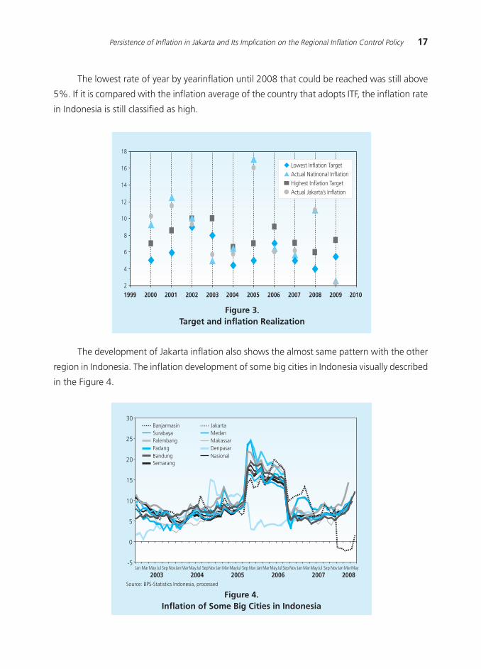
The development of Jakarta inflation also shows the almost same pattern with the other
region in Indonesia. The inflation development of some big cities in Indonesia visually described
in the Figure 4.
Figure 4.Inflation of Some Big Cities in Indonesia
-5
0
5
10
15
20
25
30BanjarmasinSurabayaPalembangPadangBandungSemarang
JakartaMedanMakassarDenpasarNasional
2003 2004 2005 2006 2007 2008Jan MarMay Jul Sep NovJan MarMayJul SepNov Jan MarMayJul Sep Nov Jan MarMayJul Sep Nov Jan MarMayJul Sep Nov Jan MarMay
Source: BPS-Statistics Indonesia, processed
18
16
14
12
10
8
6
4
2
1999 2000 2001 2002 2003 2004 2005 2006 2007 2008 2009 2010
Lowest Inflation Target
Highest Inflation TargetActual Natinonal Inflation
Actual Jakarta»s Inflation
18 Bulletin of Monetary, Economics and Banking, July 2011
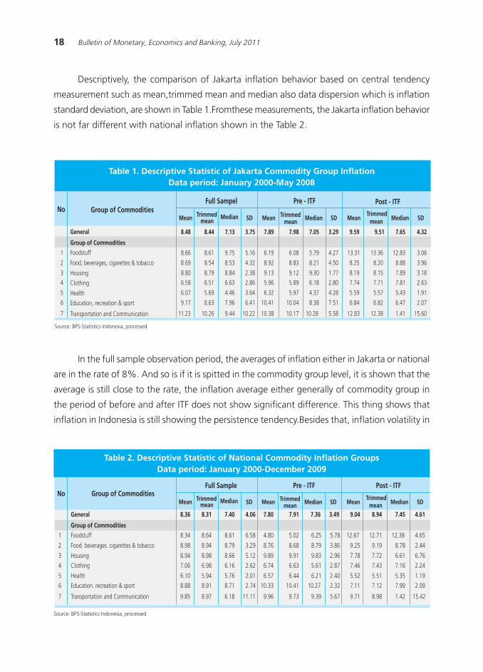
Descriptively, the comparison of Jakarta inflation behavior based on central tendency
measurement such as mean,trimmed mean and median also data dispersion which is inflation
standard deviation, are shown in Table 1.Fromthese measurements, the Jakarta inflation behavior
is not far different with national inflation shown in the Table 2.
In the full sample observation period, the averages of inflation either in Jakarta or national
are in the rate of 8%. And so is if it is spitted in the commodity group level, it is shown that the
average is still close to the rate, the inflation average either generally of commodity group in
the period of before and after ITF does not show significant difference. This thing shows that
inflation in Indonesia is still showing the persistence tendency.Besides that, inflation volatility in
Table 1. Descriptive Statistic of Jakarta Commodity Group InflationData period: January 2000-May 2008
Source: BPS-Statistics Indonesia, processed
Mean Trimmedmean
Median SD Mean Trimmedmean Median SD Mean
Trimmedmean Median SD
8.48 8.44 7.13 3.75 7.89 7.98 7.05 3.29 9.59 9.51 7.65 4.32
1 8.66 8.61 9.75 5.16 6.19 6.08 5.79 4.27 13.31 13.36 12.83 3.06
2 8.69 8.54 8.53 4.32 8.92 8.83 8.21 4.50 8.25 8.20 8.88 3.96
3 8.80 8.79 8.84 2.38 9.13 9.12 9.30 1.77 8.19 8.15 7.89 3.18
4 6.58 6.51 6.63 2.86 5.96 5.89 6.18 2.80 7.74 7.71 7.81 2.63
5 6.07 5.69 4.46 3.64 6.32 5.97 4.37 4.28 5.59 5.57 5.43 1.91
6 9.17 8.63 7.96 6.41 10.41 10.04 8.38 7.51 6.84 6.82 6.47 2.07
7 11.23 10.26 9.44 10.22 10.38 10.17 10.28 5.58 12.83 12.38 1.41 15.60
Pre - ITFNo
Full Sampel Post - ITFGroup of Commodities
General
Group of Commodities
Foodstuff
Food, beverages, cigarettes & tobacco
Housing
Clothing
Health
Education, recreation & sport
Transportation and Communication
Mean Trimmedmean
Median SD Mean Trimmedmean Median SD Mean
Trimmedmean Median SD
Pre - ITF Post - ITFNo Group of Commodities
Full Sample
General 8.36 8.31 7.40 4.06 7.80 7.91 7.36 3.49 9.04 8.94 7.45 4.61
Group of Commodities
1 Foodstuff 8.34 8.64 8.61 6.58 4.80 5.02 6.25 5.78 12.67 12.71 12.38 4.65
2 Food. beverages. cigarettes & tobacco 8.98 8.94 8.79 3.29 8.76 8.68 8.79 3.86 9.25 9.19 8.78 2.44
3 Housing 8.94 8.98 8.66 5.12 9.89 9.91 9.83 2.96 7.78 7.72 6.61 6.76
4 Clothing 7.06 6.98 6.16 2.62 6.74 6.63 5.61 2.87 7.46 7.43 7.16 2.24
5 Health 6.10 5.94 5.76 2.01 6.57 6.44 6.21 2.40 5.52 5.51 5.35 1.19
6 Education. recreation & sport 8.88 8.91 8.71 2.74 10.33 10.41 10.27 2.32 7.11 7.12 7.99 2.09
7 Transportation and Communication 9.85 8.97 6.18 11.11 9.96 9.73 9.39 5.67 9.71 8.98 1.42 15.42
Table 2. Descriptive Statistic of National Commodity Inflation GroupsData period: January 2000-December 2009
Source: BPS-Statistics Indonesia, processed
19Persistence of Inflation in Jakarta and Its Implication on the Regional Inflation Control Policy
both of the periods is not changing significantly.The existence of the shock in the Transportation
and Communication group which was triggered by the raise of natural gas in 2005 became
one of the sources of the high of inflation standard deviation in the groups.
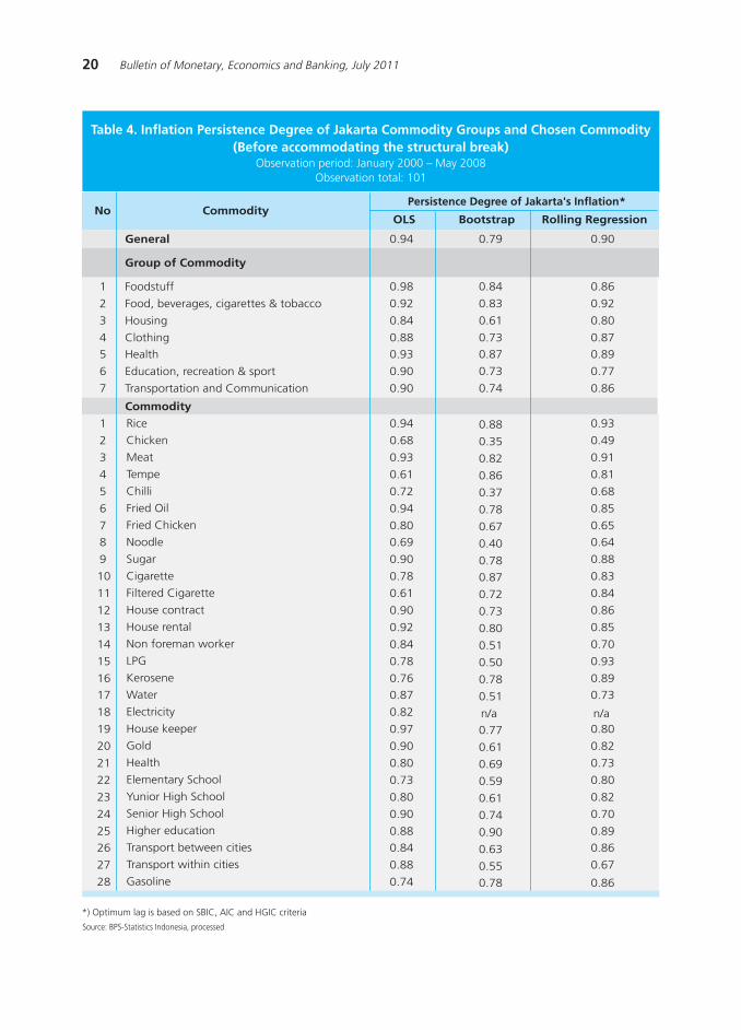
4.2 The Measurement of Jakarta Inflation Persistence Degree2
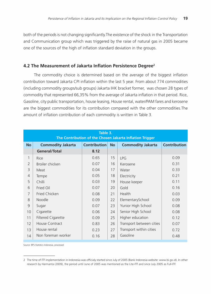
The commodity choice is determined based on the average of the biggest inflation
contribution toward Jakarta CPI inflation within the last 5 year. From about 774 commodities
(including commodity groups/sub groups) Jakarta IHK bracket former, was chosen 28 types of
commodity that represented 66,35% from the average of Jakarta inflation in that period. Rice,
Gasoline, city public transportation, house leasing, House rental, water/PAM fares and kerosene
are the biggest commodities for its contribution compared with the other commodities.The
amount of inflation contribution of each commodity is written in Table 3.
2 The time of ITF implementation in Indonesia was officialy started since July of 2005 (Bank Indonesia website: www.bi.go.id). In otherresearch by Harmanta (2009), the period until June of 2005 was mentioned as the Lite-ITF and since July 2005 as Full-ITF.
Table 3.The Contribution of the Chosen Jakarta Inflation Trigger
Source: BPS-Statistics Indonesia, processed
No Commodity Jakarta Contribution No
General/Total 8.12
1 0.65 15 0.09
2 0.07 16 0.31
3 0.04 17 0.33
4 0.05 18 0.21
5 0.03 19 0.11
6 0.07 20 0.16
7 0.08 21 0.03
8 0.09 22 0.09
9 0.07 23 0.08
10 0.06 24 0.08
11 0.09 25 0.12
12 0.83 26 0.07
13 0.23 27 0.72
14 0.16 28 0.48
Commodity Jakarta Contribution
Rice
Broiler chicken
Meat
Tempe
Chilli
Fried Oil
Fried Chicken
Noodle
Sugar
Cigarette
Filtered Cigarette
House Contract
House rental
Non foreman worker
LPG
Kerosene
Water
Electricity
House keeper
Gold
Health
ElementarySchool
Yunior High School
Senior High School
Higher education
Transport between cities
Transport within cities
Gasoline
20 Bulletin of Monetary, Economics and Banking, July 2011
Table 4. Inflation Persistence Degree of Jakarta Commodity Groups and Chosen Commodity(Before accommodating the structural break)
Observation period: January 2000 √ May 2008Observation total: 101
OLS Bootstrap Rolling Regression
General 0.94 0.79 0.90
Group of Commodity
1 Foodstuff 0.98 0.84 0.86
2 Food, beverages, cigarettes & tobacco 0.92 0.83 0.92
3 Housing 0.84 0.61 0.80
4 Clothing 0.88 0.73 0.87
5 Health 0.93 0.87 0.89
6 Education, recreation & sport 0.90 0.73 0.77
7 Transportation and Communication 0.90 0.74 0.86
Commodity
1 0.94 0.88 0.93
2 0.68 0.35 0.49
3 0.93 0.82 0.91
4 0.61 0.86 0.81
5 0.72 0.37 0.68
6 0.94 0.78 0.85
7 0.80 0.67 0.65
8 0.69 0.40 0.64
9 0.90 0.78 0.88
10 0.78 0.87 0.83
11 0.61 0.72 0.84
12 0.90 0.73 0.86
13 0.92 0.80 0.85
14 0.84 0.51 0.70
15 0.78 0.50 0.93
16 0.76 0.78 0.89
17 0.87 0.51 0.73
18 0.82 n/a n/a19 0.97 0.77 0.80
20 0.90 0.61 0.82
21 0.80 0.69 0.73
22 0.73 0.59 0.80
23 0.80 0.61 0.82
24 0.90 0.74 0.70
25 0.88 0.90 0.89
26 0.84 0.63 0.86
27 0.88 0.55 0.67
28 0.74 0.78 0.86
*) Optimum lag is based on SBIC, AIC and HGIC criteria
Persistence Degree of Jakarta's Inflation*No Commodity
Rice
Chicken
Meat
Tempe
Chilli
Fried Oil
Fried Chicken
Noodle
Sugar
Cigarette
Filtered Cigarette
House contract
House rental
Non foreman worker
LPG
Kerosene
Water
Electricity
House keeper
Gold
Health
Elementary School
Yunior High School
Senior High School
Higher education
Transport between cities
Transport within cities
Gasoline
Source: BPS-Statistics Indonesia, processed
21Persistence of Inflation in Jakarta and Its Implication on the Regional Inflation Control Policy
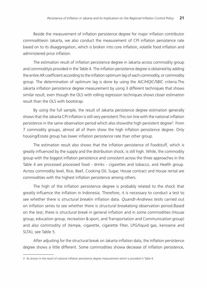
Beside the measurement of inflation persistence degree for major inflation contributor
commoditiesin Jakarta, we also conduct the measurement of CPI inflation persistence rate
based on to its disaggregation, which is broken into core inflation, volatile food inflation and
administered price inflation.
The estimation result of inflation persistence degree in Jakarta across commodity group
and commodityis provided in the Table 4. The inflation persistence degree is obtained by adding
the entire AR coefficient according to the inflation optimum lag of each commodity, or commodity
group. The determination of optimum lag is done by using the AIC/HQIC/SBIC criteria.The
Jakarta inflation persistence degree measurement by using 3 different techniques that shows
similar result, even though the OLS with rolling regression techniques shows closer estimation
result than the OLS with bootstrap.
By using the full sample, the result of Jakarta persistence degree estimation generally
shows that the Jakarta CPI inflation is still very persistent.This isin line with the national inflation
persistence in the same observation period which also showsthe high persistent degree3. From
7 commodity groups, almost all of them show the high inflation persistence degree. Only
housing/Estate group has lower inflation persistence rate than other group.
The estimation result also shows that the inflation persistence of Foodstuff, which is
greatly influenced by the supply and the distribution shock, is still high. While, the commodity
group with the biggest inflation persistence and consistent across the three approaches in the
Table 4 are processed processed food - drinks - cigarettes and tobacco, and Health group.
Across commodity level, Rice, Beef, Cooking Oil, Sugar, House contract and House rental are
commodities with the highest inflation persistence among others.
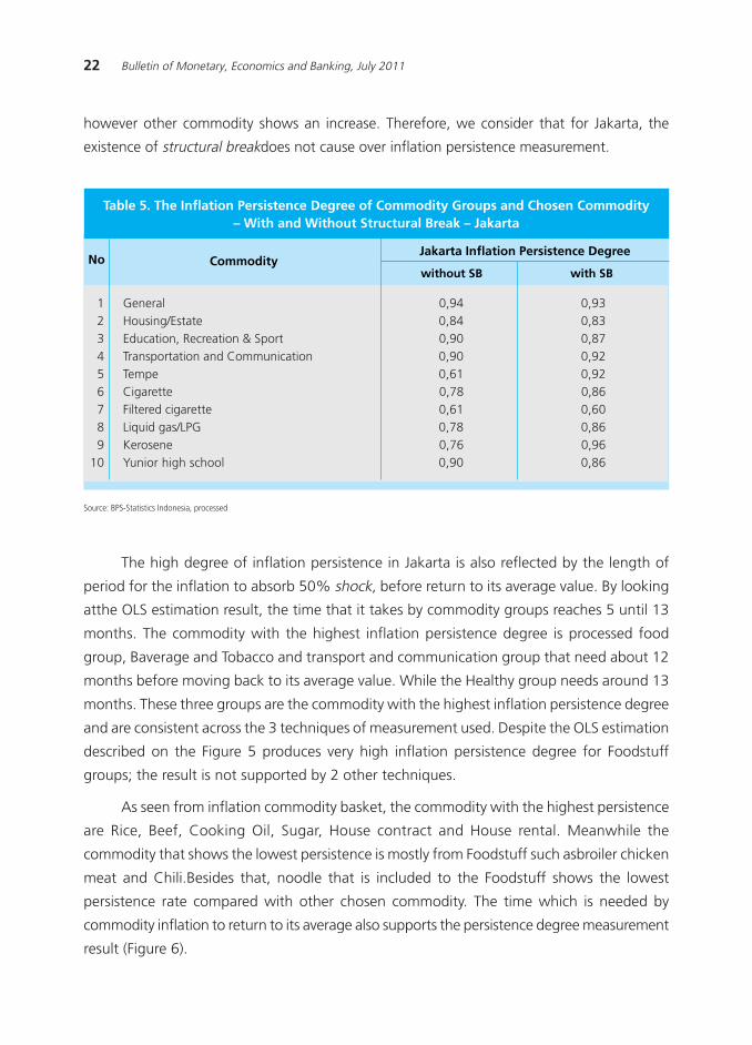
The high of the inflation persistence degree is probably related to the shock that
greatly influence the inflation in Indonesia. Therefore, it is necessary to conduct a test to
see whether there is structural breakin inflation data. Quandt-Andrews testis carried out
on inflation series to see whether there is structural breakalong observation period.Based
on the test, there is structural break in general inflation and in some commodities (House
group, education group, recreation & sport, and Transportation and Communication group)
and also commodity of (tempe, cigarette, cigarette filter, LPG/liquid gas, kerosene and
SLTA), see Table 5.
After adjusting for the structural break on Jakarta inflation data, the inflation persistence
degree shows a little different. Some commodities showa decrease of inflation persistence,
3 As shown in the result of national inflation persistence degree measurement which is provided in Table 4.
22 Bulletin of Monetary, Economics and Banking, July 2011
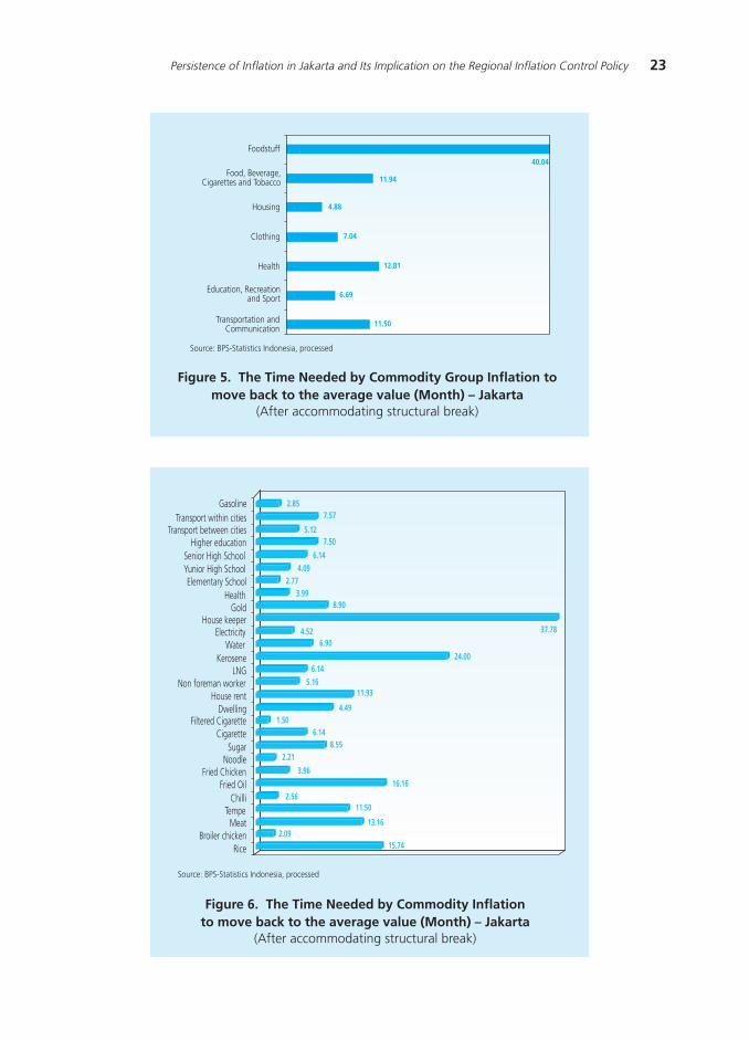
The high degree of inflation persistence in Jakarta is also reflected by the length of
period for the inflation to absorb 50% shock, before return to its average value. By looking
atthe OLS estimation result, the time that it takes by commodity groups reaches 5 until 13
months. The commodity with the highest inflation persistence degree is processed food
group, Baverage and Tobacco and transport and communication group that need about 12
months before moving back to its average value. While the Healthy group needs around 13
months. These three groups are the commodity with the highest inflation persistence degree
and are consistent across the 3 techniques of measurement used. Despite the OLS estimation
described on the Figure 5 produces very high inflation persistence degree for Foodstuff
groups; the result is not supported by 2 other techniques.
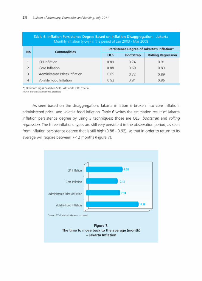
As seen from inflation commodity basket, the commodity with the highest persistence
are Rice, Beef, Cooking Oil, Sugar, House contract and House rental. Meanwhile the
commodity that shows the lowest persistence is mostly from Foodstuff such asbroiler chicken
meat and Chili.Besides that, noodle that is included to the Foodstuff shows the lowest
persistence rate compared with other chosen commodity. The time which is needed by
commodity inflation to return to its average also supports the persistence degree measurement
result (Figure 6).
Table 5. The Inflation Persistence Degree of Commodity Groups and Chosen Commodity√ With and Without Structural Break √ Jakarta
NoJakarta Inflation Persistence Degree
1 General 0,94 0,932 Housing/Estate 0,84 0,833 Education, Recreation & Sport 0,90 0,874 Transportation and Communication 0,90 0,925 Tempe 0,61 0,926 Cigarette 0,78 0,867 Filtered cigarette 0,61 0,608 Liquid gas/LPG 0,78 0,869 Kerosene 0,76 0,96
10 Yunior high school 0,90 0,86
Commodity
Source: BPS-Statistics Indonesia, processed
without SB with SB
however other commodity shows an increase. Therefore, we consider that for Jakarta, the
existence of structural breakdoes not cause over inflation persistence measurement.
23Persistence of Inflation in Jakarta and Its Implication on the Regional Inflation Control Policy
Figure 5. The Time Needed by Commodity Group Inflation tomove back to the average value (Month) √ Jakarta
(After accommodating structural break)
Figure 6. The Time Needed by Commodity Inflationto move back to the average value (Month) √ Jakarta
(After accommodating structural break)
11.94
40.04
4.88
7.04
12.81
6.69
11.50
Foodstuff
Food, Beverage,Cigarettes and Tobacco
Housing
Clothing
Health
Education, Recreationand Sport
Transportation andCommunication
Source: BPS-Statistics Indonesia, processed
2.857.57
5.127.50
6.144.09
2.773.99
8.90
4.526.90
6.145.16
11.93
4.491.50
6.148.55
2.21
3.96
2.56
2.0915.74
13.16
11.50
16.16
24.00
37.78
GasolineTransport within cities
Transport between citiesHigher education
Senior High SchoolYunior High SchoolElementary School
HealthGold
House keeperElectricity
WaterKerosene
LNGNon foreman worker
House rentDwelling
Filtered CigaretteCigarette
SugarNoodle
Fried ChickenFried Oil
ChilliTempe
MeatBroiler chicken
Rice
Source: BPS-Statistics Indonesia, processed
24 Bulletin of Monetary, Economics and Banking, July 2011
OLS Bootstrap Rolling Regression
Persistence Degree of Jakarta's Inflation*No Commodities
1 CPI Inflation 0.89 0.74 0.91
2 Core Inflation 0.88 0.69 0.89
3 Administered Prices Inflation 0.89 0.72 0.89
4 Volatile Food Inflation 0.92 0.81 0.86
*) Optimum lag is based on SBIC, AIC and HGIC criteria
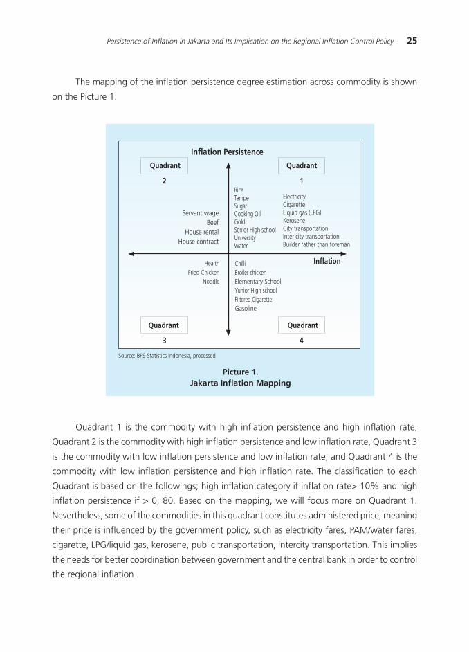
As seen based on the disaggregation, Jakarta inflation is broken into core inflation,
administered price, and volatile food inflation. Table 6 writes the estimation result of Jakarta
inflation persistence degree by using 3 techniques; those are OLS, bootstrap and rolling
regression. The three inflations types are still very persistent in the observation period, as seen
from inflation persistence degree that is still high (0.88 - 0.92), so that in order to return to its
average will require between 7-12 months (Figure 7).
Figure 7.The time to move back to the average (month)
√ Jakarta Inflation
Table 6. Inflation Persistence Degree Based on Inflation Disaggregation √ JakartaMonthly inflation (y-o-y) in the period of Jan 2003 - Mar 2008
Source: BPS-Statistics Indonesia, processed
8.28
7.13
7.74
11.98
CPI Inflation
Core Inflation
Administered Prices Inflation
Volatile Food Inflation
Source: BPS-Statistics Indonesia, processed
25Persistence of Inflation in Jakarta and Its Implication on the Regional Inflation Control Policy
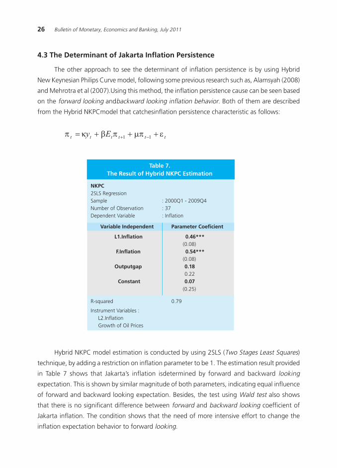
The mapping of the inflation persistence degree estimation across commodity is shown
on the Picture 1.
Picture 1.Jakarta Inflation Mapping
Quadrant 1 is the commodity with high inflation persistence and high inflation rate,
Quadrant 2 is the commodity with high inflation persistence and low inflation rate, Quadrant 3
is the commodity with low inflation persistence and low inflation rate, and Quadrant 4 is the
commodity with low inflation persistence and high inflation rate. The classification to each
Quadrant is based on the followings; high inflation category if inflation rate> 10% and high
inflation persistence if > 0, 80. Based on the mapping, we will focus more on Quadrant 1.
Nevertheless, some of the commodities in this quadrant constitutes administered price, meaning
their price is influenced by the government policy, such as electricity fares, PAM/water fares,
cigarette, LPG/liquid gas, kerosene, public transportation, intercity transportation. This implies
the needs for better coordination between government and the central bank in order to control
the regional inflation .
Quadrant
2
Inflation Persistence
Quadrant
1
Quadrant
3
Quadrant
4
Inflation
Servant wageBeef
House rentalHouse contract
HealthFried Chicken
Noodle
RiceTempeSugarCooking OilGoldSenior High schoolUniversityWater
ElectricityCigaretteLiquid gas (LPG)KeroseneCity transportationInter city transportationBuilder rather than foreman
ChilliBroiler chickenElementary SchoolYunior High schoolFiltered CigaretteGasoline
Source: BPS-Statistics Indonesia, processed
26 Bulletin of Monetary, Economics and Banking, July 2011
NKPC2SLS RegressionSample : 2000Q1 - 2009Q4Number of Observation : 37Dependent Variable : Inflation
Variable Independent Parameter Coeficient
L1.Inflation 0.46***(0.08)
F.Inflation 0.54***(0.08)
Outputgap 0.180.22
Constant 0.07(0.25)
R-squared 0.79
Instrument Variables : L2.Inflation Growth of Oil Prices
4.3 The Determinant of Jakarta Inflation Persistence
The other approach to see the determinant of inflation persistence is by using Hybrid
New Keynesian Philips Curve model, following some previous research such as, Alamsyah (2008)
and Mehrotra et al (2007).Using this method, the inflation persistence cause can be seen based
on the forward looking andbackward looking inflation behavior. Both of them are described
from the Hybrid NKPCmodel that catchesinflation persistence characteristic as follows:
Table 7.The Result of Hybrid NKPC Estimation
Hybrid NKPC model estimation is conducted by using 2SLS (Two Stages Least Squares)
technique, by adding a restriction on inflation parameter to be 1. The estimation result provided
in Table 7 shows that Jakarta»s inflation isdetermined by forward and backward looking
expectation. This is shown by similar magnitude of both parameters, indicating equal influence
of forward and backward looking expectation. Besides, the test using Wald test also shows
that there is no significant difference between forward and backward looking coefficient of
Jakarta inflation. The condition shows that the need of more intensive effort to change the
inflation expectation behavior to forward looking.
27Persistence of Inflation in Jakarta and Its Implication on the Regional Inflation Control Policy
Meanwhile, output gap data is obtained by using HP filter technique. The estimation
showsthe output gap parameter is not significant to influence the inflation.In other word, the
output gap influence toward inflation has not been concluded yet.
The high inflation causes negative impact toward the economy. The high inflation will
give the uncertainty for economic agent in making decision beside influence the purchasing
power of society especially those with constant expectation. The economy management will
be more difficult if the inflation rate is persistent. By definition, the flow of inflation will take
more time before return to the its initial rate prior the shock. In addition, the inflation will also
require longer time to converge. These will amplify the effort needed to decrease the inflation
rate. Since Jakarta has the biggest weight in forming national inflation, then the high inflation
persistence in Jakarta implicates high effort to decrease national inflation.
Based on these assessment, the high inflation persistence degree in Jakarta is because of
the volatile food and administered price groups. This imply the need of stronger coordination
between the government and Bank Indonesia to control the inflation. While for the administered
price group is higly depends on the government effort to arrange the timing and the magnitude
of the price (and income) policy so that its impact toward inflation is minimum.
The high volatile food and administered price inflation will influence the influence
expectation, hence complicates the regional inflation control. Good coordination through the
existing coordination forums such as Bank Indonesia Governor council coordination meeting
with the government, inflation target stipulation forum, also forward looking inflation controlling
team, needs to be more optimized. Regarding to the Team for Monitoring and Controlling the
Regional Inflation / Tim Pemantauan dan Pengendalian Inflasi Daerah (TPID), its target to cover
all region in Indonesia (66 cities) needs to be monitored, considering its importance to reach
low and stable national inflation.
Beside that the TPID role can be optimized if it involve inter-regional coordination, especially
between the region with high economic linkage. In addition, TPID should realize its role to
provide information system (database) in monitoring the biggest inflation contributor commodity,
which is useful in determining price policy in regional level.
The effort to control inflation in region is subsequently can give positive impact toward
faster inflation convergence across region, hence the regional inflation can be easier to controlled.
The inflation control through monetary policy in national level, then is expected to be more
effective. The issue of convergence and coordination across region especially Jakarta and other
region should be interesting topic for next paper4.
4 Arimurti and Trisnanto, ≈Inter regional inflation convergence in Indonesia∆, forthcoming paper.
28 Bulletin of Monetary, Economics and Banking, July 2011
The inflation pressure sourced mainly from inflation expectation especially backward
looking one implies a more intensive dissemination of information and central bank policy to
direct the economic agent expectation to be forward looking, in order to achieve the low and
stable inflation. These attempts are also related to the credibility of policy maker that needs to
be strengthened and maintained.
5. SUMMARY
This research gives several important conclusions, first, the empirical test shows the CPI
inflation in Jakarta is persistent. Similar result is shown in a more disaggregated group, where
the administered price inflation, and volatile food inflation in Jakarta is classified to be very
persistent .Comodity groups with highest degree of persistence are Processed Foods, Beverages
and Tobaccos and Health. On commodity level, Rice, Beef, Cooking Oil, Sugar, and Dwelling.
In Jakarta, the comodity group mostly need 5-12 months to return to its average prior the
shock, while for the mostly commodity needs between 3-12 months. Second, in accordance
with the hybrid NKPC model result, it is found that the Jakarta»s inflation is a combination
between forward and backward looking behavior, This is in line with the result of national
inflation behavior (Alamsyah, 2008). Third, the cause of high inflation persistence degree in
Jakarta are because of the high of inflation persistence degree of volatile food and administered
price groups. This volatile food and administered price inflation affect the inflation expectation,
hence will complicate the inter regional inflation control.
This findings has several policy implications; first,the needsto intensify the dissemination
of information and policy in order to direct inflation expectation to be more on forward looking.
Second, the need to optimizethe coordination between the government and the Central Bank
through the existing coordination forums such as Bank Indonesia governor council coordination
meeting with government, inflation target stipulation forum, and also inflation controlling
team.
29Persistence of Inflation in Jakarta and Its Implication on the Regional Inflation Control Policy
REFERENCES
Alamsyah, H. (2008). Inflation Persistance and Its Impact Towards Choice and Respond of
Monetary Policy in Indonesia
Angeloni, I., Aucremanne, L., Ehrmann, M., Gali, J., Levin, A., & Smets, F. (2004). Inflation
Persistence in the Euro Area : Preliminary Summary of Findings.
Babecky, J., CorRicelly, F., & Horvath, R. (2008, June). Assessing Inflation Peristence: Micro
Evidence on an Inflation Targeting Economy. CERGE-EI .
Batini, N. (2002, December). Euro Area Inflation Persistence. European Central Bank Working
Paper Series .
Debelle, G., & Wilkinson, J. (2002). Inflation Targeting and the Inflation Process: Some Lessons
from an Open Economy. Research Bank of Australia - Research Discussion Paper 2002-01 .
Dossche, M., & Everaert, G. (2005, June). Measuring Inflation Persistence: A Structural Time
Series Approach. National Bank of Belgium Working Paper .
Federal Reserve Bank of San Fransisco. (2006, October 13). Inflation Persistence in an Era of
Well-Anchored Inflation Expectations. FRBSF Economic Letter .
Harmanta. (2009). Monetary Policy Credibilityand its impact towardsInflation Persistence and
Disinflation Strategy in Indonesia: with Dynamic Stochastic General Equilibrium (DSGE) Model.
Jakarta: Faculty of Business and Economics,Post Graduate Program ofEconomic Science,
University of Indonesia.
Levin, A. T., & Piger, J. M. (2004, April). Is Inflation Persistence Intrinsic in Industrial Economies?
European Central Bank Working Paper Series .
Marques, C. R. (2005). Inflation Peristence: Facts or Artefacts? Economic Bulletin .
Marques, C. R. (2004, June). Inflation Persistence: Facts or Artefacts? European Central Bank
Working Paper Series .
O»Reilly, G., & Whelan, K. (2004, April). Has Euro-Area Inflation Persistence Change Over Time?
European Central Bank Working Paper Series .
Pivetta, F., & Reis, R. (2006). The Persistence of Inflation in the United States. Journal of Economic
Dynamics and Control , April.
Stock, J. H. (2004, December). Inflation Persistence in the Euro Area: Evidence from Aggregate
and Sectoral Data.

30 Bulletin of Monetary, Economics and Banking, July 2011
Tim Inflasi. (2007). Core Inflation Persistence. Strategic Issue. Governor Council Meeting
Materials, 4 January. Jakarta: Bank Indonesia.
Willis, J. L. (2003). Implications of Structural Changes in the U.S. Economy for Pricing Behavior
and Inflation Dynamics. Federal Reserve Bank of Kansas City Economic Review .
Yanuarti, T. (2007). Has Inflation Persistence in Indonesia Changed?
31Sovereign Risk Analysis of Developing Countries: Findings From Credit Default Swap Premium Behaviour
SOVEREIGN RISK ANALYSIS OF DEVELOPING COUNTRIES:FINDINGS FROM CREDIT DEFAULT SWAP PREMIUM BEHAVIOUR
Moch. Doddy Ariefianto dan Soenartomo Soepomo 1
This study conducts econometric analysis CDS Premium relations towards variables usually used
as a sovereign rating explanatory. Estimation with data panel econometric found that global risk appetite
is the most important influencing variable followed by foreign exchange reserve and yield spread. This
item is consistent with the existing empiric literature and shows a high correlation between developing
countries economy and world economic cycle.
JEL Classification : F34, F32, G13, G15, C23
Keywords::::: Sovereign Risk, Credit Default Swap, Panel Data
1 The authors are lecturer in Economic and Business Faculty, University of Ma Chung, Malang; [email protected] [email protected] .
Abstract
32 Bulletin of Monetary, Economics and Banking, July 2011
I. INTRODUCTION
Foreign debt has already become important source of fund in developing countries. This
external financing is needed in order to fill the saving-investment gap that is usually negative.
Foreign debt can be in any forms such as government debt, government bond, corporate
bond, bilateral-multilateral loan, etc.
The price of the loan depends on the scheme, economic condition (fiscal and monetary),
and reputation. In some decades recently, there is a kind of institution trend that does
specialization in debt valuation. This institution, which is always called as rating agency institution,
measures the ability of certain entity, quantitatively and qualitatively, to pay (credit risk) and
give this entity a ranking. Special for sovereign entity, the rating has been established since
1975 by Standard and Poor»s (Beers and Cavanaugh, 2006).
Credit risk measurement is not actually new. A credit risk model in default probability
form has been formulated by Altman with his famous Z-statistics in 1968. The development
of credit risk modeling is already advanced including its sophisticated statistic technique and
calibration of variables used. Cantor (2004) gave a review about the credit risk modeling.
The sovereign risk is important and attracting a huge attention of investors. Unlike
private credit risk, investor cannot seize the collateral or government income when event
default occurs. That is why the credit valuation for government loans becomes more
important.
As credit corporate risk, sovereign risk can also be influenced by domestic and
international condition (Beers and Cavanaugh, 2006), including economic or political condition.
Fiscal pressure, for instance, caused by large outstanding debt and government deficit, can
force the government to delay the installment and interest payment as well as the regime
transformation caused by political turbulence. The ruling government today can reject the
debt from previous government.
Interaction pattern of modern economic nowadays has a very high interrelation one
another. Practically, there are no countries that can isolate their economy from external shock.
Subprime mortgage crisis in the US in 2007 and the world economic contraction during
2008-2009 are the real evidences in terms of high interrelation among countries. Thus, a
country can experience an economic crisis as the impact of external turbulence, and make
the existing government to restructure their loan payment.
Further innovation in credit risk management in the early 21st century is the emergence
of Credit Default Swap (CDS). This derivative instrument has a function like bond insurance.
33Sovereign Risk Analysis of Developing Countries: Findings From Credit Default Swap Premium Behaviour
CDS holder (called as protection buyer) can exchange his bond with the sum of nominal face
value, to CDS seller (protection seller) in the case of default (Taylor, 2007). To get this protection,
CDS buyer must pay a certain premium (stated in percentage of debt).
Figure 1.CDS Development
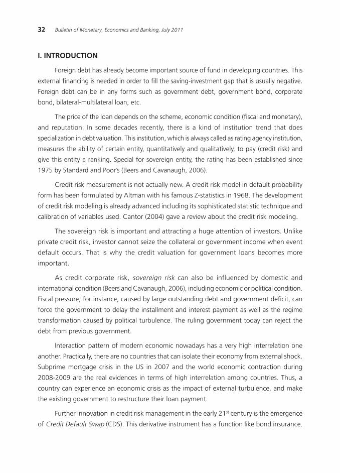
Data from Bank for International Settlement (BIS) shows, since firstly introduced in 2005,
CDS contract value has achieved USD 41.9 Trillion as for December 2008 (Figure 1). Even with
rapid development, CDS position is considered too small among other derivative instruments.
Interest derivative, for instance, is valued at USD 403 at the same period. Even its reputation is
deceived by negative impact from the subprime mortgage, Hull (2011) predicted that this
instrument has a bright prospect in the future.
Sovereign CDS for developing countries is started within the same period. There is a
high correlation between CDS movement with the change of a country»s rating (Ismailescu and
Kazemi, 2010). Thus, the based rating change can explain the CDS movement. Furthermore,
CDS is potential to be leading indicator for financial market.
This research is conducted to reveal the relation between CDS and sovereign rating as
its explanatory variables. The outcome of the study is expected to benefit not only academician,
700
600
500
400
300
200
100
0Dec June
2005Dec June
2006Dec June
2007Dec June
2008Dec
(USD trilions, December 2001 - December 2008)
(USD 41,9 trilion in,December 2008)
Credit Default Swaps
Commodity ContractsEquity-Linked Contracts
Credit Default SwapsForeign Exchange Contracts
700
600
500
400
300
200
100
0
34 Bulletin of Monetary, Economics and Banking, July 2011
(1)
but also for policy maker.This paper consists of five sections. Next section presents the theory
and empirical literature about CDS. The third section explains the methodology of research
including our empirical scheme. The forth section discusses result and analysis, while conclusion
and policy implication will close the presentation.
II. THEORY
2.1. CDS Valuation Overview
Duffie (1999) suggested to considering CDS as swap default able floating rate notes
towards default free floating rate note. As a swap, the owner of CDS has a right to exchange
his default-able instruments with the cash flow from default free instrument that belongs to
swap seller. This swap is triggered when the credit event occur. The credit event can be in any
forms such as outright default from underlying securities issuer, restructuring, rescheduling, or
even just the postponement of interest/installment payment (Hull, 2011).
Skinner and Townend (2002), in the other hand, used a put option approach in valuing
CDS. As a put option, CDS buyer has a right to sell securities that belong to him at par value
when credit event occurred. Furthermore, they also explained that CDS premium meet the put
and call parity:
Where X is noticed as strike price from the option (par value), B is noticed as a security that
contain credit risk, p is CDS premium, D is coupon value, and r is interest rate of risk free
portfolio. They showed that this inequality will be fulfilled, so that the CDS premium is analogue
to the premium of an option.
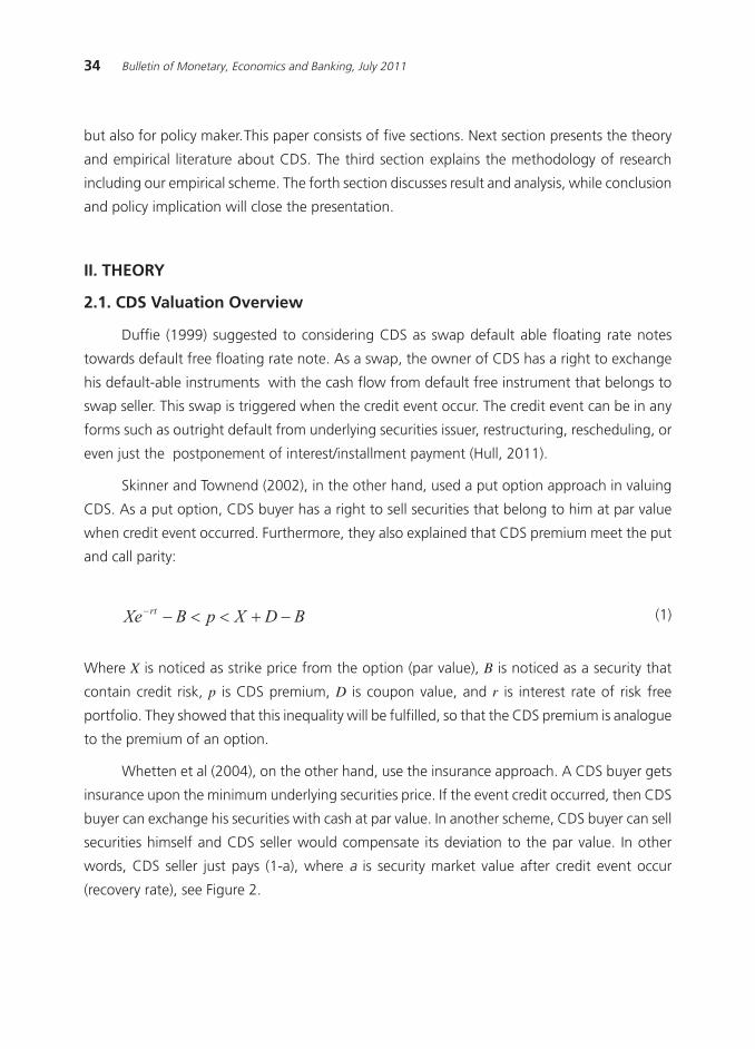
Whetten et al (2004), on the other hand, use the insurance approach. A CDS buyer gets
insurance upon the minimum underlying securities price. If the event credit occurred, then CDS
buyer can exchange his securities with cash at par value. In another scheme, CDS buyer can sell
securities himself and CDS seller would compensate its deviation to the par value. In other
words, CDS seller just pays (1-a), where a is security market value after credit event occur
(recovery rate), see Figure 2.
35Sovereign Risk Analysis of Developing Countries: Findings From Credit Default Swap Premium Behaviour
Figure 2. CDS Scheme
By using the approach from Whetten et al (2004), the premium from CDS can be measured
as follow:
1. There are 2 types of cash flow from CDS transaction, which are fixed premium payment
from CDS buyer and contingency cash flow that is paid by CDS seller only if credit event
occurred.
2. CDS value (for buyer) is the present value of all contingency cash flow minus fixed cash
flow.
3. Fixed cash flow depends on nominal premium on each period and survival ability2 . If premium
is noticed as S, di is payment period (as an annual fraction), q(t
i) is survival rate and D(t
i) is
adjusted discount factor, then the present value can be formulated as follow3:
CDS Spreads
(bps)
ProtectionBuyer Protection
Seller
1 - Recovery rate(%)
Reference Entity
Trigger Event
Source : Whetten et al (2004)
2 If credit event happens, then CDS buyer does not need to pay. Thus there is probability that in a period, CDS buyer does not need topay premium because the credit event happens. One minus this probability is called survivalability.
3 The second part of formula 2 is premium payment accrual value if default occurs between payment period ti-1
and ti.
(2)
36 Bulletin of Monetary, Economics and Banking, July 2011
4 Most of material in this part are summarized from Beers and Cavanaugh (2006)
4. Whereas the number of contingency cash flow can be calculated as a difference of recovery
rate (R) from the par value, or
(3)
5. In equilibrium condition, premium value will equalize the fixed and contingency cash flow
payment, or explicitly stated:
(4)
6. With a little math, we can obtain the CDS premium valuation as follow:
(5)
2.2. Sovereign Rating Approach Towards CDS Premium4
Sovereign rating is credit risk evaluation for government entity, and not specifically for
certain issuer. The rating reflects credit risk evaluation for all entities in a country. The other
credit risk entity would always be smaller or equal with sovereign rating. Thus, the sovereign
rating becomes very important since the domestic credit price will be affected if the sovereign
rating degrades.
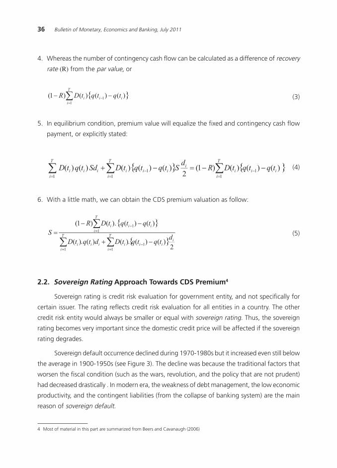
Sovereign default occurrence declined during 1970-1980s but it increased even still below
the average in 1900-1950s (see Figure 3). The decline was because the traditional factors that
worsen the fiscal condition (such as the wars, revolution, and the policy that are not prudent)
had decreased drastically . In modern era, the weakness of debt management, the low economic
productivity, and the contingent liabilities (from the collapse of banking system) are the main
reason of sovereign default.
37Sovereign Risk Analysis of Developing Countries: Findings From Credit Default Swap Premium Behaviour
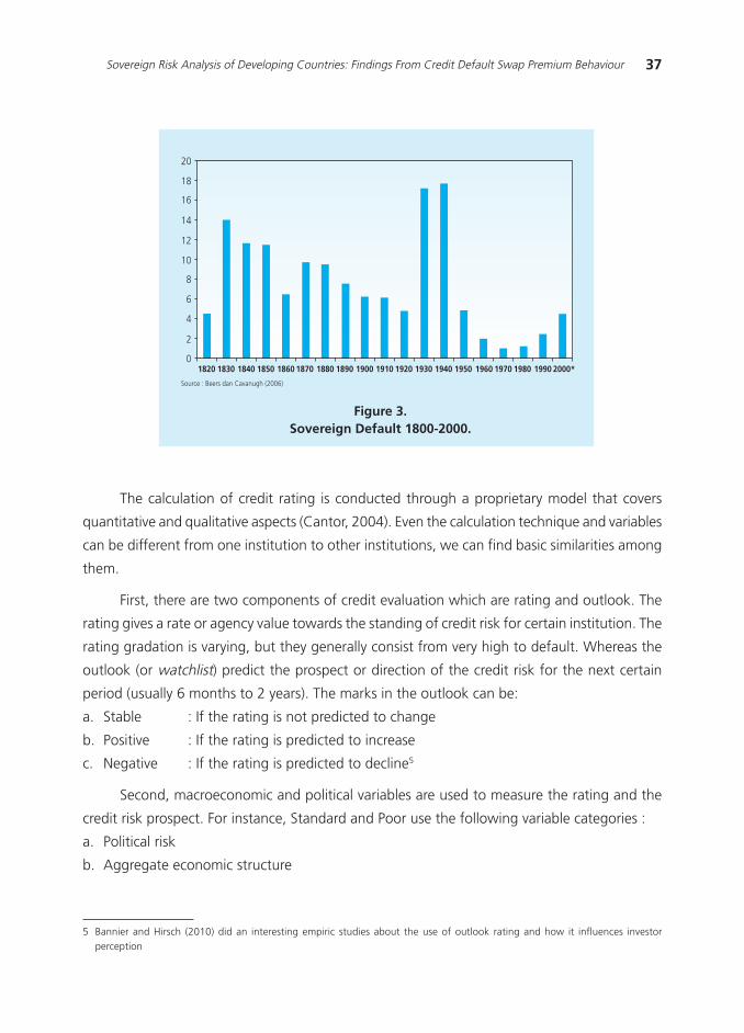
The calculation of credit rating is conducted through a proprietary model that covers
quantitative and qualitative aspects (Cantor, 2004). Even the calculation technique and variables
can be different from one institution to other institutions, we can find basic similarities among
them.
First, there are two components of credit evaluation which are rating and outlook. The
rating gives a rate or agency value towards the standing of credit risk for certain institution. The
rating gradation is varying, but they generally consist from very high to default. Whereas the
outlook (or watchlist) predict the prospect or direction of the credit risk for the next certain
period (usually 6 months to 2 years). The marks in the outlook can be:
a. Stable : If the rating is not predicted to change
b. Positive : If the rating is predicted to increase
c. Negative : If the rating is predicted to decline5
Second, macroeconomic and political variables are used to measure the rating and the
credit risk prospect. For instance, Standard and Poor use the following variable categories :
a. Political risk
b. Aggregate economic structure
Figure 3.Sovereign Default 1800-2000.
5 Bannier and Hirsch (2010) did an interesting empiric studies about the use of outlook rating and how it influences investorperception
20
18
16
14
12
10
8
6
4
2
0
Source : Beers dan Cavanugh (2006)
1820 1830 1840 1850 1860 1870 1880 1890 1900 1910 1920 1930 1940 1950 1960 1970 1980 1990 2000*
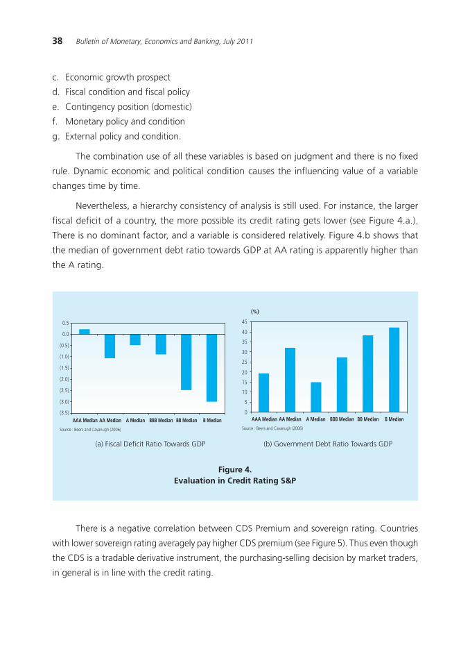
38 Bulletin of Monetary, Economics and Banking, July 2011
c. Economic growth prospect
d. Fiscal condition and fiscal policy
e. Contingency position (domestic)
f. Monetary policy and condition
g. External policy and condition.
The combination use of all these variables is based on judgment and there is no fixed
rule. Dynamic economic and political condition causes the influencing value of a variable
changes time by time.
Nevertheless, a hierarchy consistency of analysis is still used. For instance, the larger
fiscal deficit of a country, the more possible its credit rating gets lower (see Figure 4.a.).
There is no dominant factor, and a variable is considered relatively. Figure 4.b shows that
the median of government debt ratio towards GDP at AA rating is apparently higher than
the A rating.
Figure 4.Evaluation in Credit Rating S&P
(a) Fiscal Deficit Ratio Towards GDP (b) Government Debt Ratio Towards GDP
AAA Median AA Median A Median BBB Median BB Median B Median
Source : Beers and Cavanugh (2006)
0.5
0.0
(0.5)
(1.0)
(1.5)
(2.0)
(2.5)
(3.0)
(3.5)AAA Median AA Median A Median BBB Median BB Median B Median
Source : Beers and Cavanugh (2006)
45
40
35
30
25
20
15
10
5
0
(%)
There is a negative correlation between CDS Premium and sovereign rating. Countries
with lower sovereign rating averagely pay higher CDS premium (see Figure 5). Thus even though
the CDS is a tradable derivative instrument, the purchasing-selling decision by market traders,
in general is in line with the credit rating.
39Sovereign Risk Analysis of Developing Countries: Findings From Credit Default Swap Premium Behaviour
Figure 5.Correlation between CDS Premium and Sovereign Rating S&P.
2.3. Empirical Studies Review
Considering that CDS is a new instrument that has just been actively traded, empirical
study exploring this product is not much done yet. Skinner and Townend (2002) use linear
regression approach on analyzing CDS premium. By assuming CDS as a put option, they
estimated a linear model that relates premium with standard variables explaining price option
such as interest rate of risk free asset, yield, and underlying instrument volatility, maturity
and strike price (artificial).
Data used are 20 realization spots of CDS trade sovereign in US during September 1997
and 1999. After calculating the impact of Asian Crisis, they found that 4 of 5 variable coefficients
are significant with correct signs.
Weigel and Gemmil (2006) built a special instrument (called distance to default) from
statistical process, for 4 developing countries yield; Argentina, Brazil, Mexico, and Venezuela.
As explanatory variables, they use various economic and market indicator that are categorized
as global, regional, and country specific. They found that country specific variable only explained
8% of the dependent variance. The biggest part (45%) is explained by regional factor especially
through financial market integration. Amounted 20% is influenced by global factor (using
proxy of US stock exchange return). The rest 20% variance cannot be explained by explanatory
variable of the model.
0
200
400
600
800
1000
BB- BB BB+ BBB- BBB+ A-
Venezuela
Latvia
Romania
Panama IndiaThailand Malaysia
Philippines
TurkeyIndonesia
Vietnam Egypt
Morocco
Kazakhstan
Hungary
Brazil
Colombia
Peru
40 Bulletin of Monetary, Economics and Banking, July 2011
One of the leading indicators about economic problems encountered by a country is the
exchange rate. Thus, it can be naturally predicted that there is a positive correlation between
the exchange rate pressures with the CDS. This hypothesis has been verified by Carr and Wu
(2007). By using a weekly data of Brazil and Mexico (In January 2002 until March 2005), they
estimated relation between exchange rate risk variance with CDS premium through joint-diffusion
model. The result of their studies showed that the CDS movement intensity is higher than the
exchange rate return variance. It indicates that CDS is over estimate than its real default
probability.
A study that measures the reaction of CDS sovereign of developing countries towards
the credit rating movement (Standard and Poor) is done by Ismailescu and Kazemi (2010). They
used data set consisted of 22 countries with daily frequency on 2 January 2001 until 22 April
2009. The dependent variable is CDS change as a function of a dummy for credit event and a
group of control variables. There are 2 types of dummy, one for the credit event on certain
country (country credit event) and the other is credit event for one block countries (regional
credit event).
They found that credit rating event is not symmetric. A positive change announcement
gives a direct impact meanwhile the negative one gives no impact. It indicates that the positive
announcement gives more information than the negative one. CDS premium has an ability to
predict the credit rating event for downgrade rating (negative) but not for the upgrading one
(positive). The last, credit rating event will have a stronger spillover impact if the rating change
is positive instead of negative.
Matsumura and Vicente (2010) started a studies focusing on default probability (latent
variable) of Brazil by using five variables macroeconomic explanatory, namely the Fed interest
rate, VIX: implied volatility index S&P 500, real exchange rate, stock exchange index (Ibovespa)
and interest rate swap. Daily data in period 17 February 1999 until 15 September 2004 (1320
days) is used to estimate empirical model. They found that The Fed interest rate and VIX is the
most important factor in explaining the change of default probability on Brazil securities.
Bannier and Hirsch (2010) made an interesting empirical study focusing on economic
function from credit outlook announcement. They use all senior unsecured debt data issued
by US government and is rated by Moodys. Overall, the sample has 4043 observation; consist
of 2531 upgrades and 1512 downgrades. Econometrics model used is panel linear with
Cumulative Absolute Return (CAR) as dependent variable and 7 explanatory variables where
some of them are upgrade/downgrade point (in notches) and out/in category dummy of
investment grade.
41Sovereign Risk Analysis of Developing Countries: Findings From Credit Default Swap Premium Behaviour
They found that the downgrade rating gives higher market respond compared when
issuer gets into watchlist. Empirical findings also support the implicit contract hypothesis (Boot
et al, 2006). In this hypothesis, watchlist has economic function to coordinate investor perception
and to direct the issuer»s perception.
Our study has several differences from previous studies , first, our empirical model is
simpler. Using reduce form, we directly estimate the relationship between CDS premium and
macroeconomic variables through price determinant variables (maturity, volatility, free risk interest
rate, etc.). This parsimonious model is expected to give more intuitive insight. Second, we use
larger set of developing countries panel data, from which we expect to have more comprehensive
result.
III. METHODOLOGY
We employ linear panel data model to link the CDS and its explanatory variables . The
empirical model is specified as follow:
Where Sit is 5 years CDS premium of country i on a period t, α is intercept model, X is the
vector of explanatory variables and εit is residual component. We assume the residual component
is only one way that came from cross section heterogeneity. Thus, εit can be classified into two
components which are cross section type component (vi) and idiosyncratic error (u
it). Residual
heterogeneity can be in fixed constant form (Fixed Effect, FE) or random (Random Effect, RE).
We apply the Redundant fixed effect likelihood ratio test to choose the most appropriate
heterogeneity model.
There are 9 explanatory variables used in this study6. Definition, operational proxy, and
relation sign expectation (hypothesis) is given in table 1. 10 developing countries are used as
cross section with observation period covers 2004 until 2009 in an annual frequency. Those
countries are Indonesia, Columbia, Hungarian, Malaysia, Peru, Philippine, Thailand, Turkey,
Venezuela, and Vietnam. Thus, there are 60 observations in this study.
6 Some of variables in this research such as CDS, foreign exchange reserve, and VIX are converted in natural log form. It is intended tomake those coefficient of estimation can be interpreted as an elasticity.
42 Bulletin of Monetary, Economics and Banking, July 2011
Table 1.Variables Used In Conducting Studies
No. Variabel Description, Proxy dan Notation Expected Sign
1 Credit Default Swap
2 Economic Growth
3 Inflation
4 Depreciation
5 Yield Spread
6 Government Debt
7 Foreign ExchangeReserve
8 Fiscal Deficit
9 Current Account Deficit
10 Global Risk Appetite
CDS Premium with 5 years tenor
Annual change percentage (year on year). RealGDP. (GROWGROWGROWGROWGROW)
Annual price rate change percentage (year onyear) of consumer (INFLATIONINFLATIONINFLATIONINFLATIONINFLATION)
Annual exchange rate change percentage(towards USD) (year on year) (DEPRDEPRDEPRDEPRDEPR)
Difference between government notes payableinterest rate and US Treasury in 5 years tenor(Y_SPREADY_SPREADY_SPREADY_SPREADY_SPREAD)
Government debt ration towards nominal GDP(DEBT)DEBT)DEBT)DEBT)DEBT)
State foreign exchange reserve value i on thelast of the year t (in billion USD, DEVISADEVISADEVISADEVISADEVISA)
Ratio between government fiscal deficit towardsnominal GDP (FIS_DEFFIS_DEFFIS_DEFFIS_DEFFIS_DEF)
Ration between current accountcurrent accountdeficit towards nominal GDP (CA_DEFCA_DEFCA_DEFCA_DEFCA_DEF)
VIX index value, implied volatility from putoption index Standard & Poor»s (VIXVIXVIXVIXVIX)
Dependent Variable
Negative
Positive
Positive
Negative
Positive
Negative
Positive
Positive
Positive
IV. RESULT AND ANALYSIS
We firstly explain descriptive statistics from variables used. Then we will reveal the result
of estimation gained and also analytic interpretation.
4.1. Descriptive Statistics
Table 2 shows descriptive statistics (all samples) from the used variables in the model.
As predicted, CDS premium, foreign exchange reserve, and exchange rate depreciation are
variables with the largest range. Meanwhile fiscal deficit and current account deficit are
relatively stable.
43Sovereign Risk Analysis of Developing Countries: Findings From Credit Default Swap Premium Behaviour
On Table 3, the highest average of CDS premium is in Venezuela (865 bps), while the
lowest is in Malaysia (71 bps). The macroeconomic management pattern of these countries
varies one another. For instance Hungarian and Philippine are slightly loose in managing their
fiscal as indicated by the fiscal deficit ratio and debt that respectively reaches -6.25% and
68%, and 2.17% and 64.8%.
Table 2.Used Descriptive Statistics Variables
Variable Mean Median Maximum Minimum Deviation Std
CDS 5CDS 5CDS 5CDS 5CDS 5 256.6918 167.0000 3218.044 16.23000 433.0109
GROWGROWGROWGROWGROW 4.826263 5.040000 18.28700 -6.730000 4.143712
INFLATIONINFLATIONINFLATIONINFLATIONINFLATION 8.839252 6.514625 31.90000 -11.34632 8.549880
DEPRDEPRDEPRDEPRDEPR -0.329263 -0.544737 30.98265 -17.71857 9.601061
Y_SPREADY_SPREADY_SPREADY_SPREADY_SPREAD 5.188258 4.288700 21.63010 -0.909300 4.296805
DEBTDEBTDEBTDEBTDEBT 44.94912 43.40000 81.90000 13.90000 14.97648
DEVISADEVISADEVISADEVISADEVISA 41.37088 33.13500 137.8000 12.63100 28.12098
FIS_DEFFIS_DEFFIS_DEFFIS_DEFFIS_DEF -1.992982 -1.900000 9.500000 -9.300000 2.955555
CA_DEFCA_DEFCA_DEFCA_DEFCA_DEF 1.272193 0.100000 17.88700 -11.91800 7.430450
VIXVIXVIXVIXVIX 20.56754 21.68000 40.00000 11.56000 10.09849
Source: Bloomberg, IMF and World Bank
Table 3.Descriptive Statistics Across Country
Countries CDS5Y Debt Fis_def Y_spread Grow CA_def Depr Devisa Inflation
Columbia 201.12 46.90 -2.12 6.50 4.53 -2.08 -4.68 18.67 21.97
Hungarian 122.63 67.92 -6.25 4.35 1.30 -6.89 -1.00 26.38 5.30
Malaysia 70.94 44.82 -3.12 0.24 4.19 14.97 -1.71 84.85 2.83
Peru 176.42 32.60 1.03 2.71 6.62 0.05 -2.85 22.67 -1.52
Philippines 264.57 64.82 -2.17 4.56 4.76 3.18 -2.61 25.40 5.89
Thailand 86.24 42.67 -0.43 0.67 3.37 1.49 -2.67 80.76 3.23
Turkey 215.30 46.48 -2.62 10.66 3.95 -4.60 2.11 58.08 8.62
Venezuela 865.31 23.83 1.08 7.41 8.36 11.52 5.33 25.88 21.97
Vietnam 184.21 34.18 -5.63 5.13 7.28 -6.04 2.87 16.03 11.40
Indonesia 289.02 42.42 -0.92 7.14 5.31 1.75 2.37 48.05 8.56
Source: Bloomberg, IMF and World Bank
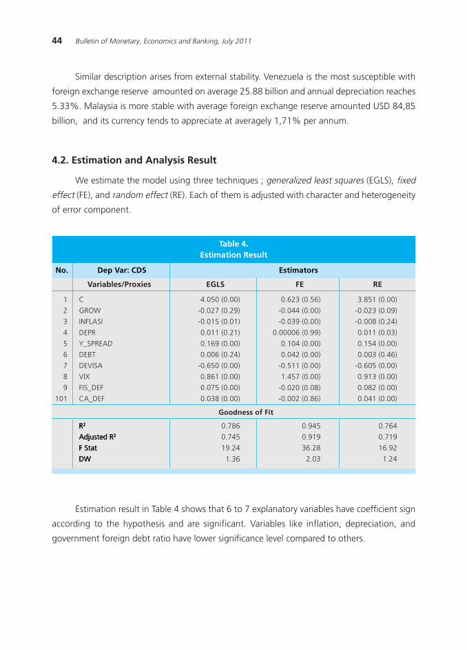
44 Bulletin of Monetary, Economics and Banking, July 2011
Similar description arises from external stability. Venezuela is the most susceptible with
foreign exchange reserve amounted on average 25.88 billion and annual depreciation reaches
5.33%. Malaysia is more stable with average foreign exchange reserve amounted USD 84,85
billion, and its currency tends to appreciate at averagely 1,71% per annum.
4.2. Estimation and Analysis Result
We estimate the model using three techniques ; generalized least squares (EGLS), fixed
effect (FE), and random effect (RE). Each of them is adjusted with character and heterogeneity
of error component.
Table 4.Estimation Result
No. Dep Var: CDS Estimators
1 C 4.050 (0.00) 0.623 (0.56) 3.851 (0.00)
2 GROW -0.027 (0.29) -0.044 (0.00) -0.023 (0.09)
3 INFLASI -0.015 (0.01) -0.039 (0.00) -0.008 (0.24)
4 DEPR 0.011 (0.21) 0.00006 (0.99) 0.011 (0.03)
5 Y_SPREAD 0.169 (0.00) 0.104 (0.00) 0.154 (0.00)
6 DEBT 0.006 (0.24) 0.042 (0.00) 0.003 (0.46)
7 DEVISA -0.650 (0.00) -0.511 (0.00) -0.605 (0.00)
8 VIX 0.861 (0.00) 1.457 (0.00) 0.913 (0.00)
9 FIS_DEF 0.075 (0.00) -0.020 (0.08) 0.082 (0.00)
101 CA_DEF 0.038 (0.00) -0.002 (0.86) 0.041 (0.00)
Goodness of Fit
RRRRR22222 0.786 0.945 0.764
Adjusted RAdjusted RAdjusted RAdjusted RAdjusted R22222 0.745 0.919 0.719
F StatF StatF StatF StatF Stat 19.24 36.28 16.92
DWDWDWDWDW 1.36 2.03 1.24
Variables/Proxies EGLS FE RE
Estimation result in Table 4 shows that 6 to 7 explanatory variables have coefficient sign
according to the hypothesis and are significant. Variables like inflation, depreciation, and
government foreign debt ratio have lower significance level compared to others.
45Sovereign Risk Analysis of Developing Countries: Findings From Credit Default Swap Premium Behaviour
The goodness of fit rate of empirical model is good. The independent variables are
able to simultaneously explain the existing 76% until 94% variation of CDS premium. F-
statistic test are over the critical value indicating variables use in the model gives additional
information.
VIX variable has the biggest coefficient, which is from 0.861 (EGLS) until 1.457 (FE).
Considering that this coefficient represents the elasticity, and then a 1% of global risk
perception increase encourages the increase of CDS by 0.861% to 1.457%. This findings
confirmed earlier study from Matsumura and Vicente (2010) as explained above. CDS as a
risky asset class will experience decrease in demand when world market sentiment worsen.
It also shows the integration level in derivative market in to world economic cycle.
Foreign exchange reserve is significant on the model. Estimated coefficient shows
that each 1% increase of foreign exchange reserve will be followed by the decrease of CDS
by 0.511% (EGLS) to 0.651% (FE). The role of foreign exchange reserve towards economic
stability is highly important. First generation crisis theory expressed by Krugman (1979) and
Flood and Garber (1984) shows how an attack towards exchange rate triggered by the low
foreign exchange reserve. The empirical findings give support to the first generation crisis
theory.
Yield spread variable with US treasury (that is comparable) becomes the third biggest
influencing variable. Each of 1% increase of yield spread will give impact to the CDS increase
by 0.104% to 0.169%. Yield spread is actually a sovereign risk measurement, because
yield is the sum of real interest rate (opportunity cost of money) and risk premium.
Nevertheless, considering that yield curve is also a monetary policy tool then it is not perfect
measure of risk.
Economic development, inflation, depreciation, debt ratio, fiscal deficit ratio, and
current account give smaller impact but some of them remain significant. These variables
are country economic specific. Thus, it can be seen indeed that these internal explanatory
variables contribute limitedly; it accords to Weigel and Gemmil findings (2006).
Overall, the empirical sign and its significance have supported hypothesis expressed
in this research. CDS as a market instrument has a connection to fundamental economic
variables (global and domestic). Thus, the movement of CDS also reflects trader perception
towards the economic prospects (sovereign risk). Furthermore, considering that this
instrument is daily traded, it is possible to use it as leading indicator for sovereign risk
prospect.
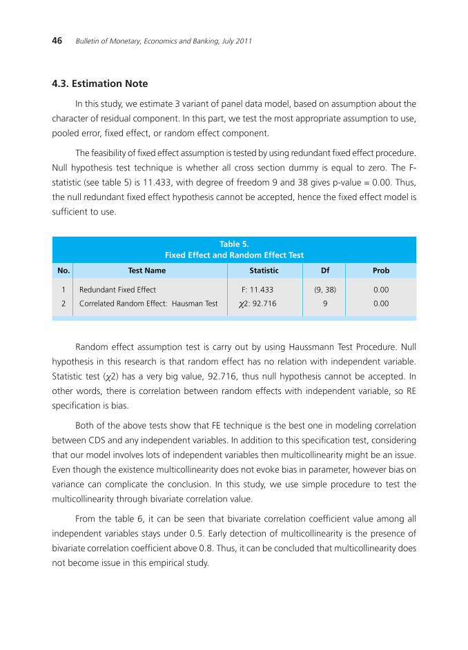
46 Bulletin of Monetary, Economics and Banking, July 2011
Table 5.Fixed Effect and Random Effect Test
No. Test Name Statistic Df Prob
1 Redundant Fixed Effect F: 11.433 (9, 38) 0.00
2 Correlated Random Effect: Hausman Test χ2: 92.716 9 0.00
4.3. Estimation Note
In this study, we estimate 3 variant of panel data model, based on assumption about the
character of residual component. In this part, we test the most appropriate assumption to use,
pooled error, fixed effect, or random effect component.
The feasibility of fixed effect assumption is tested by using redundant fixed effect procedure.
Null hypothesis test technique is whether all cross section dummy is equal to zero. The F-
statistic (see table 5) is 11.433, with degree of freedom 9 and 38 gives p-value = 0.00. Thus,
the null redundant fixed effect hypothesis cannot be accepted, hence the fixed effect model is
sufficient to use.
Random effect assumption test is carry out by using Haussmann Test Procedure. Null
hypothesis in this research is that random effect has no relation with independent variable.
Statistic test (χ2) has a very big value, 92.716, thus null hypothesis cannot be accepted. In
other words, there is correlation between random effects with independent variable, so RE
specification is bias.
Both of the above tests show that FE technique is the best one in modeling correlation
between CDS and any independent variables. In addition to this specification test, considering
that our model involves lots of independent variables then multicollinearity might be an issue.
Even though the existence multicollinearity does not evoke bias in parameter, however bias on
variance can complicate the conclusion. In this study, we use simple procedure to test the
multicollinearity through bivariate correlation value.
From the table 6, it can be seen that bivariate correlation coefficient value among all
independent variables stays under 0.5. Early detection of multicollinearity is the presence of
bivariate correlation coefficient above 0.8. Thus, it can be concluded that multicollinearity does
not become issue in this empirical study.
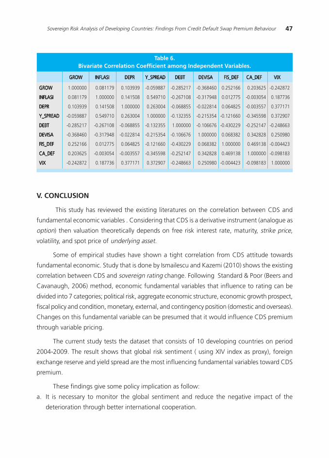
47Sovereign Risk Analysis of Developing Countries: Findings From Credit Default Swap Premium Behaviour
V. CONCLUSION
This study has reviewed the existing literatures on the correlation between CDS and
fundamental economic variables . Considering that CDS is a derivative instrument (analogue as
option) then valuation theoretically depends on free risk interest rate, maturity, strike price,
volatility, and spot price of underlying asset.
Some of empirical studies have shown a tight correlation from CDS attitude towards
fundamental economic. Study that is done by Ismailescu and Kazemi (2010) shows the existing
correlation between CDS and sovereign rating change. Following Standard & Poor (Beers and
Cavanaugh, 2006) method, economic fundamental variables that influence to rating can be
divided into 7 categories; political risk, aggregate economic structure, economic growth prospect,
fiscal policy and condition, monetary, external, and contingency position (domestic and overseas).
Changes on this fundamental variable can be presumed that it would influence CDS premium
through variable pricing.
The current study tests the dataset that consists of 10 developing countries on period
2004-2009. The result shows that global risk sentiment ( using XIV index as proxy), foreign
exchange reserve and yield spread are the most influencing fundamental variables toward CDS
premium.
These findings give some policy implication as follow:
a. It is necessary to monitor the global sentiment and reduce the negative impact of the
deterioration through better international cooperation.
Table 6.Bivariate Correlation Coefficient among Independent Variables.
GROWGROWGROWGROWGROW INFLASIINFLASIINFLASIINFLASIINFLASI DEPRDEPRDEPRDEPRDEPR Y_SPREADY_SPREADY_SPREADY_SPREADY_SPREAD DEBTDEBTDEBTDEBTDEBT DEVISADEVISADEVISADEVISADEVISA FIS_DEFFIS_DEFFIS_DEFFIS_DEFFIS_DEF CA_DEFCA_DEFCA_DEFCA_DEFCA_DEF VIXVIXVIXVIXVIX
GROWGROWGROWGROWGROW Ω1.000000 Ω0.081179 Ω0.103939 -0.059887 -0.285217 -0.368460 Ω0.252166 Ω0.203625 -0.242872
INFLASIINFLASIINFLASIINFLASIINFLASI Ω0.081179 Ω1.000000 Ω0.141508 Ω0.549710 -0.267108 -0.317948 Ω0.012775 -0.003054 Ω0.187736
DEPRDEPRDEPRDEPRDEPR Ω0.103939 Ω0.141508 Ω1.000000 Ω0.263004 -0.068855 -0.022814 Ω0.064825 -0.003557 Ω0.377171
Y_SPREADY_SPREADY_SPREADY_SPREADY_SPREAD -0.059887 Ω0.549710 Ω0.263004 Ω1.000000 -0.132355 -0.215354 -0.121660 -0.345598 Ω0.372907
DEBTDEBTDEBTDEBTDEBT -0.285217 -0.267108 -0.068855 -0.132355 Ω1.000000 -0.106676 -0.430229 -0.252147 -0.248663
DEVISADEVISADEVISADEVISADEVISA -0.368460 -0.317948 -0.022814 -0.215354 -0.106676 Ω1.000000 Ω0.068382 Ω0.342828 Ω0.250980
FIS_DEFFIS_DEFFIS_DEFFIS_DEFFIS_DEF Ω0.252166 Ω0.012775 Ω0.064825 -0.121660 -0.430229 Ω0.068382 Ω1.000000 Ω0.469138 -0.004423
CA_DEFCA_DEFCA_DEFCA_DEFCA_DEF Ω0.203625 -0.003054 -0.003557 -0.345598 -0.252147 Ω0.342828 Ω0.469138 Ω1.000000 -0.098183
VIXVIXVIXVIXVIX -0.242872 Ω0.187736 Ω0.377171 Ω0.372907 -0.248663 Ω0.250980 -0.004423 -0.098183 Ω1.000000

48 Bulletin of Monetary, Economics and Banking, July 2011
b. Sufficient foreign exchange reserve is necessary as a buffer if an immediate negative shock
occur. High foreign exchange reserve can also become a signal of external sector credibility
and stability.
c. Monitoring any movement of bond in the market is highly important. Yield spread is an
indicator towards sovereign risk perception change.
49Sovereign Risk Analysis of Developing Countries: Findings From Credit Default Swap Premium Behaviour
REFERENCES
Bank for International Settlement, Triennial Quarterly Survey, Derivative Market, September
2010.
Bannier, C.E., and Hirsch, C.W., 2010, ≈The economic function of credit rating agencies √
What does the watch list tell us?∆ Journal of Banking and Finance, Vol. 34, page. 3037-
3049.
Beers, D.T and M. Cavanaugh, 2006, Sovereign Credit Ratings: A Primer, 2006, Standard &
Poor»s Research.
Cameroon, A.C., and Triverdi., P. K., 2005, Micro econometrics: Methods and Applications,
Cambridge, New York.
Cantor, R., 2004,»≈An Introduction to recent research on credit ratings∆, Journal of Banking
and Finance, Vol 28, page. 2565-2573.
Carr, P., and Wu, L., 2007,∆Theory and evidence on the dynamic interactions between sovereign
credit swaps and currency option∆, Vol. 31, page 2383-2403.
Hull, J.C., 2011, Fundamentals Of Futures and Options Market., 7th Edition, Pearson.
Ismailescu, I and Kazemi, H., 2010,∆≈The reaction of emerging market credit default swap
spreads to sovereign credit rating changes∆, Journal of International Banking & Finance,
Vol. 34, page 2861-2873.
Matsumura, M.S. and Vicente, J.V.M, 2010,∆≈The role of macroeconomic variables in sovereign
risk∆, Emerging Markets Review, 11, page 229-249.
Nomura, Fixed Income Research Team, Credit Default Swap Primer, May 2004.
Skinner, F.S and Townend, T.G., 2002,∆An empirical analysis of credit default swaps∆,
International Review of Financial Analysis, Vol. 11, page. 297-309.
Weigel, D.D. and Gemmill, G., 2006, ≈What drives credit risk in emerging markets? The roles
of country fundamentals and market co-movements ≈, Journal of International Money and
Finance, 25, page 476-502.
Whetten, M., Adelson M., and Van Bemmelen, 2004,≈≈Credit Default Swap: A Primer∆, Nomura
Fixed Income Research.

50 Bulletin of Monetary, Economics and Banking, July 2011
This page is intentionally left blank
51Determinant of Bank Runs In Indonesia: Bad Luck or Fundamental?
DETERMINANT OF BANK RUNS IN INDONESIA:BAD LUCK OR FUNDAMENTAL?
Iskandar Simorangkir 1
This paper examine the determinant of bank runs in Indonesia that includes economic fundamental,
bank performance, and self-fulfilling prophecy factors for all banks either in full sample periods between
years 1990 √ 2005 or in banking crisis periods between years 1997 √ 1998. The bank runs determinant
uses dynamic panel model from Arrelano-Bond. Estimation result shows that self-fulfilling prophecy, bank
monetary performance which is rentability and fixed credit ratio and macroeconomic condition which is
economic growth, inflation and real exchange rate influence bank runs in Indonesia. Bank runs determinant
in banking crisis between year 1997 √ 1998 also shows a result that is not really different from bank runs
determinant during full sample periods between years 1990 √ 2005.
1 Head of Economi Research Bureau, Bank Indonesia and lecturer at Postgraduate Program University of Pelita Harapan Jakarta. Thewriter is grateful to Prof. Rustam Didong, Dr. Muliaman Hadad, and Dr. Sugiharso Safuan upon the ideas. All parts in this article arethe subjective points of view of the writer
Abstract
Classification JEL: : : : : C29, C33, G21
Key Words: Bank runs, Banking Crisis, Arrelano Bond Dynamic Panel
52 Bulletin of Monetary, Economics and Banking, July 2011
I. INTRODUCTION
Bank runs is a phenomenon where many customers withdraw their money in a great
amount together and immediately in a bank because costumers do not believe that the bank is
able to fully pay the money on time2. Bank runs occurring in a bank would become a crisis if it
spreads to other banks (contagious effect). Bank runs and banking crisis have become a global
phenomenon and occurred repeatedly in both developed and developing countries within the
last decades. Bank runs and banking crisis even occurred frequently since monetary liberalization
in 1980s and 1990s (Davis and Karim, 2007). Even in the middle 2007 until today, world
money market is experiencing a global monetary crisis that came from subprime mortgage in
United States (US).
In a modern banking history, banking crisis had happened long before the World War I,
like bank runs (bank panic) and banking crisis occurred in United States in 1837, 1873, 1884,
1890, 1907, and 1933 (Calomiris, 2007). Research conducted by the IMF in 181 member
countries shows that since 1980 until mid-1996, there were 133 bank runs and a serious
banking crisis (Lindgren, Garcia and Saal, 1996). The next terrible banking crisis occurred in
1997/1998 in some of East Asian countries, including Indonesia, Thailand, Malaysia, Philippine
and South Korea. The crisis started from the exchange rate crisis in Thailand and is contagious
to Indonesia and other East Asian countries and further developed into a banking crisis and
economic crisis (Bank Indonesia, 1998). The financial crisis occurred in the U.S. occurred again
in 2007/2008 and has grown into a global financial crisis and its impact is still experienced until
now.
In the case of Indonesia, bank runs also occurred repeatedly. In 1992, there was a bank
runs on several national banks resulting liquidated Bank Summa. Subsequently, in the year
1997/1998 there was bank runs that evolved into the worst banking crisis ever in the banking
history of Indonesia. The closure of 16 banks by the Government on November 1, 1997 has
resulted in reduced customer trust for the banks, especially the private banks where public
believed they had bad financial performance. The decline of trust for the banks encouraged
customers to massively withdraw their funds (bank runs). Furthermore, withdrawal at a bank
systemically3 spread (contagion) to other banks so it evolved into a banking crisis.
2 Definition of bank runs was expressed by George G. Kaufman on The Concise Encyclopedia of Economics in websitehttp://www.econlib.org/library/Enc/BankRuns.html or in George G. Kaufman on ≈Bank runs: Causes, Benefits and Costs.∆∆Cato Journal 2,No. 3 (Winter 1988): 559-88.
3 Systemic risk is a risk where a bank runs in a bank can trigger a bank runs to other banks or in academic literature it is always calledas risk giving contagion effect. The process of systemic occurrence or the contagion happened through self-fulfilling prophecy
53Determinant of Bank Runs In Indonesia: Bad Luck or Fundamental?
Repeated phenomenon of bank runs and banking crisis are caused by the nature of
banks where they are the institutions that are vulnerable towards funds withdrawal by customers
on a large scale. The vulnerability is an impact of the operations of banks that transform short-
term liabilities, such as demand deposits, savings and time deposits into longer-term assets,
such as credit. Under these conditions, banks have always faced problems of maturity mismatch
so that it is very vulnerable to large-scale funds withdrawals (bank runs) by customers because
of the limited liquid assets owned by banks.
Subsequently, bank runs on one bank can cause a systemic risk, which is spreading to
other banks. Systemic risk occurs because customers at other banks do not know the information
about the condition of his/her bank (asymmetric information) so that customers think that their
banks also face the same problems, it makes customers massively withdraw their funds in the
banks. The same bank runs process also occurs in other banks, so there are many banks would
experience bank runs and ultimately lead to banking crises. Factors causing bank runs that
come from the worriedness (belief) of the customers due to the absence of information about
the bank»s performance is often called as self-fulfilling prophecy. Bank runs caused by a self-
fulfilling prophecy factor is a random event from the news that is not symmetrical (asymmetric
information) received by the customers (agent). The widely influential theory models were
developed by Diamond and Dybvig (1983).
Beside self-fulfilling prophecy factor, factors causing bank runs are fundamental factors,
both derived from macroeconomic and bank fundamentals (Kindleberger (1978), Gup and
Bartholomew (1999)). Shock that occurs in the economic fundamentals, such as the economic
contraction, the increase of interest rates, the exchange rate volatility, the asset impairment
and the increase of uncertainty in the financial sector, would encourage a negative effect on
the business activities of banks. Contraction or weakening economy may lead to an increase in
bad debts of banks and subsequently can lead to inability to pay the bank customer deposit
withdrawals because most of customer funds are embedded in bad debts.
Some researches show that banking crises that occurred in a country have generated a
huge loss for the economy and society (Hoelscher and Quintyn, 2003 and Hanson, 2005). The
obstruction of access to financing for business world would lead to an economic decrease or
contraction so it encourages an increase in unemployment. Besides, bank restructuring as an
attempt to recover the impact of the banking crisis also requires a large fiscal costs and will
ultimately be borne to the tax payer. The output loss experienced by the countries facing banking
crisis is various depends on how deep and long it is. Hanson (2005) conducted a study of the
output loss due to the banking crisis. The results of these studies argued that Indonesia suffered
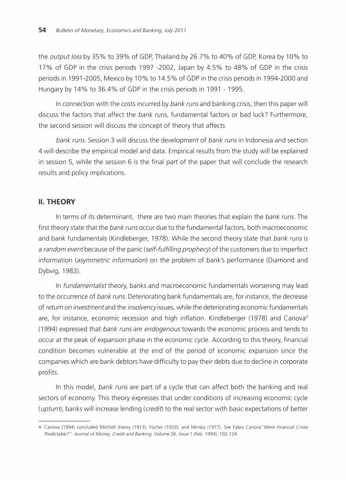
54 Bulletin of Monetary, Economics and Banking, July 2011
the output loss by 35% to 39% of GDP, Thailand by 26.7% to 40% of GDP, Korea by 10% to
17% of GDP in the crisis periods 1997 -2002, Japan by 4.5% to 48% of GDP in the crisis
periods in 1991-2005, Mexico by 10% to 14.5% of GDP in the crisis periods in 1994-2000 and
Hungary by 14% to 36.4% of GDP in the crisis periods in 1991 - 1995.
In connection with the costs incurred by bank runs and banking crisis, then this paper will
discuss the factors that affect the bank runs, fundamental factors or bad luck? Furthermore,
the second session will discuss the concept of theory that affects
bank runs. Session 3 will discuss the development of bank runs in Indonesia and section
4 will describe the empirical model and data. Empirical results from the study will be explained
in session 5, while the session 6 is the final part of the paper that will conclude the research
results and policy implications.
II. THEORY
In terms of its determinant, there are two main theories that explain the bank runs. The
first theory state that the bank runs occur due to the fundamental factors, both macroeconomic
and bank fundamentals (Kindleberger, 1978). While the second theory state that bank runs is
a random event because of the panic (self-fulfilling prophecy) of the customers due to imperfect
information (asymmetric information) on the problem of bank»s performance (Diamond and
Dybvig, 1983).
In fundamentalist theory, banks and macroeconomic fundamentals worsening may lead
to the occurrence of bank runs. Deteriorating bank fundamentals are, for instance, the decrease
of return on investment and the insolvency issues, while the deteriorating economic fundamentals
are, for instance, economic recession and high inflation. Kindleberger (1978) and Canova4
(1994) expressed that bank runs are endogenous towards the economic process and tends to
occur at the peak of expansion phase in the economic cycle. According to this theory, financial
condition becomes vulnerable at the end of the period of economic expansion since the
companies which are bank debtors have difficulty to pay their debts due to decline in corporate
profits.
In this model, bank runs are part of a cycle that can affect both the banking and real
sectors of economy. This theory expresses that under conditions of increasing economic cycle
(upturn); banks will increase lending (credit) to the real sector with basic expectations of better
4 Canova (1994) concluded Mitchell theory (1913), Fischer (1933), and Minsky (1977). See Fabio Canova≈Were Financial CrisesPredictable?∆. Journal of Money, Credit and Banking. Volume 26, Issue 1 (Feb. 1994), 102-124.
55Determinant of Bank Runs In Indonesia: Bad Luck or Fundamental?
economic growth in the future. Furthermore, banks will have a great credit (highly leveraged)
and if the cycle of economic declines, the debtor cannot repay the loan. These conditions
generated banks liquidity problems and makes those banks do not have sufficient reserves to
cover losses.
The causes of bank runs can also be derived from bank fundamental factors (Gorton,
1988). Banks will have difficulty in providing liquidity to meet its customers fund withdrawals if
the banks have poor financial performance. The occurrence of losses, poor solvency, and poor
current asset quality generate retention of customer funds on bad current assets, such as bad
credit loans. Furthermore, these conditions resulted in the lack of liquidity available at banks, so
banks are always vulnerable to bank runs.
Meanwhile, the second theory states that bank runs occur due to random events caused
by bank customers panic (agent) and is not always related to economic fundamentals. Theory
model of the second group that is widely influential was developed by Diamond and Dybvig
(1983). This model explains that the bank runs that occur are a rational response of belief of
the agent due to asymmetric information about bank performance. If the customer (agent)
thinks that the banks do not have sufficient funds to meet the customer fund withdrawal, then
bank runs will occur. A bank will face massive withdrawal if many individuals believe that other
customers will massively withdraw their funds or often refer to self-fulfilling prophecy.
In this group, including« Calomiris and Gorton (1991), they expressed a combination
factors between self-fulfilling prophecy and the shock of banking assets is the cause bank runs.
Besides that, Chen (1999) expresses that beside self-fulfilling prophecy and liquidity factors,
the moral hazard also contributes to the occurrence of bank runs. Contagion in the discussion
of bank runs is often interpreted as a factor that is equal to the self-fulfilling prophecy because
contagion means that bank runs on a bank will affect the bank runs on other banks. The
influencing process from one bank to another occurred through a withdrawal transmission
mechanism of customers (self-fulfilling prophecy). Thus according to this theory, bank runs is
mainly due to bad luck instead of fundamental factors. From the empirical side, studies of bank
runs and determinants of banking crises have been a lot done. For example, Canova (1994)
conducted a study on the determinants of banking crises in the period 1864-1914 in the U.S.
with a probit model. The results of these studies indicate that the banking crisis in U.S. in that
period was caused by the impact of economic factors. Further research also concluded that
there would be a seasonal banking crisis that is influenced by economic cycles.
Research on the determinants of banking crisis as a whole by using data panel of developing
and developed countries is conducted by Demirgüç-Kunt and Detragiache (1998). The model
56 Bulletin of Monetary, Economics and Banking, July 2011
used is a multivariate logit with the conclusion result that shows banking crises can occur if the
macroeconomic condition is weak (low economic growth and high inflation), high interest
rates, sudden capital outflow and high credit loan. Eichengreen and Rose (1998) conducted a
study of external shocks (international shock) towards banking crisis in OECD countries and the
results show that interest rates have a major influence, while economic growth has little influence
on the vulnerability of the banking crisis.
The above determinants of banking crises study is done using aggregate data from each
country (cross country) so there is the possibility of aggregation problems, such as denying
each other out factors among the banks that are aggregating. Concerning to these weaknesses,
McCandless, Gabrielli and Rouillet (2003) used individual bank data and dynamic data panel
model to determine the determinants of bank runs and banking crises in Argentina which
occurred in 2001. The research findings indicate that the determinant of bank runs that occurred
in Argentina is the factor of self-fulfilling prophecy, macroeconomic shock and worsening bank
fundamentals condition.
III. PROGRESS OF BANKING CRISIS IN INDONESIA
At first the crisis that hits Indonesia»s economy since 1997 is mainly triggered by the crisis
of the rupiah. The huge depreciation pressure of the rupiah exchange rate is mainly derived
from the factor of contagion from the crisis of the exchange rate of Thai Baht in July 1997.
Effect of contagion did not only hit Indonesia but also rapidly expanded into other Asian countries,
such as the Philippines, Malaysia and South Korea. Increasingly heavy pressure on the rupiah
depreciation forced Indonesia to remove managed floating exchange rate regime (managed
floating) to free floating exchange rate system on August 14, 1997. In order to avoid the
national economy from a deeper crisis as a result of the pressure of depreciation and capital
outflow, the government decided a package of economic policy in September 1997. Furthermore,
the program expanded to stabilization and economic reform programs supported by IMF, World
Bank, and ADB formally in November 1997. As the implementation of financial sector reform
program in order to make better banking system, then on 1 November 1997, 16 private banks
were closed.
Closure of 16 banks led to bank runs on banks where according to public perception
quite unreliable. Banks closure policy that should have been intended to recover the national
banking precisely resulted in a massive withdrawal of funds on non-government banks. Large-
scale withdrawal is due to the ruin of public trust towards banks due to bank closures policy.
The more widespread bank runs are also caused by the weak financial performance of banks,
57Determinant of Bank Runs In Indonesia: Bad Luck or Fundamental?
such as the increase in bad credit loans and declining banks rentability as the impact of
management of businesses that did not fully follow the nature of good governance. (Warjiyo,
2001 and Bank Indonesia, 19985). Besides, the rapid depreciation of rupiah resulted in ballooning
bank foreign debt denominated in rupiah. The condition was further aggravated by the absence
of guarantee program. During the absence of guarantee program and information about the
condition of banks (asymmetric information), bank customers, particularly private bank
customers, massively withdraw their funds and transfer them to a bank that considered better
and safer assets (fiat money) .
One month after the closure of 16 banks mentioned above (December 1997), the amount
of third party funds in national commercial private banks (BUSN) decreased by Rp 22.9 trillion
(11.94%). Withdrawal of funds started from the closure of banks and reached the highest
withdrawal in December 1997 and January 1998. The massive withdrawal declined since the
government provided a guarantee (blanket guarantee) in January 1998. However, when the
massive chaos occurred in May 1998, the number of banks experienced bank runs again.
In the period of banking crisis in 1997/1998, a large-scale withdrawals (bank runs)
commonly occurred in non-foreign6 exchange BUSN, frozen bank activities7, and frozen bank
operations8. Peak massive withdrawals on non-foreign exchange BUSN occurred in December
1997, January 1998, and May 1998. As an illustration, in December 1997, from 45 non-foreign
exchange BUSN, 25 bank experienced a decrease of third party»s funds by 10%, 17 banks
decreased by 20%, 13 experienced funds decline by 40%, 11 banks declined by 60%, and 6
banks experienced decreasing funds by 80% of the total amount of the previous month.
As in non-foreign exchange BUSN,»bank runs also occurred in frozen business bank (BBKU)
and frozen operation bank (BBO). The highest withdrawal occurred during November 1997
until January 1998, and March until May 1998. For instance, in November 1998, 26 banks
from 40 BBKU experienced third party funds decline by 10% from the total of previous month
third party funds, 14 banks experienced decline by 20% from the previous month amount, and
2 banks experienced decline by 40% from the previous month amount. Bank runs on BBO is
not much different from BBKU. In January 1998, from 10 BBO, 6 banks experienced third party
funds decline by 20% and 4 banks decline by 40%.
5 Annual report of Bank Indonesia in 1997/19986 Non-foreign exchange BUSNs is national private banks that are not allowed to conduct foreign exchange activities in their business
activities.7 Frozen bank activities (BBKU) is bank where its business activities is frozen or is not allowed to have any business activities temporarily
or in a certain period8 Frozen bank operation (BBO) is a bank where operational activities is frozen temporarily
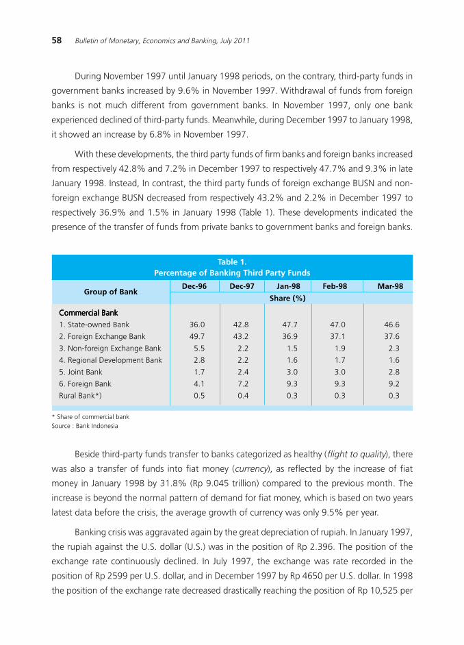
58 Bulletin of Monetary, Economics and Banking, July 2011
During November 1997 until January 1998 periods, on the contrary, third-party funds in
government banks increased by 9.6% in November 1997. Withdrawal of funds from foreign
banks is not much different from government banks. In November 1997, only one bank
experienced declined of third-party funds. Meanwhile, during December 1997 to January 1998,
it showed an increase by 6.8% in November 1997.
With these developments, the third party funds of firm banks and foreign banks increased
from respectively 42.8% and 7.2% in December 1997 to respectively 47.7% and 9.3% in late
January 1998. Instead, In contrast, the third party funds of foreign exchange BUSN and non-
foreign exchange BUSN decreased from respectively 43.2% and 2.2% in December 1997 to
respectively 36.9% and 1.5% in January 1998 (Table 1). These developments indicated the
presence of the transfer of funds from private banks to government banks and foreign banks.
* Share of commercial bankSource : Bank Indonesia
Beside third-party funds transfer to banks categorized as healthy (flight to quality), there
was also a transfer of funds into fiat money (currency), as reflected by the increase of fiat
money in January 1998 by 31.8% (Rp 9.045 trillion) compared to the previous month. The
increase is beyond the normal pattern of demand for fiat money, which is based on two years
latest data before the crisis, the average growth of currency was only 9.5% per year.
Banking crisis was aggravated again by the great depreciation of rupiah. In January 1997,
the rupiah against the U.S. dollar (U.S.) was in the position of Rp 2.396. The position of the
exchange rate continuously declined. In July 1997, the exchange was rate recorded in the
position of Rp 2599 per U.S. dollar, and in December 1997 by Rp 4650 per U.S. dollar. In 1998
the position of the exchange rate decreased drastically reaching the position of Rp 10,525 per
Group of Bank
Table 1.Percentage of Banking Third Party Funds
Commercial BankCommercial BankCommercial BankCommercial BankCommercial Bank
1. State-owned Bank 36.0 42.8 47.7 47.0 46.6
2. Foreign Exchange Bank 49.7 43.2 36.9 37.1 37.6
3. Non-foreign Exchange Bank 5.5 2.2 1.5 1.9 2.3
4. Regional Development Bank 2.8 2.2 1.6 1.7 1.6
5. Joint Bank 1.7 2.4 3.0 3.0 2.8
6. Foreign Bank 4.1 7.2 9.3 9.3 9.2
Rural Bank*) 0.5 0.4 0.3 0.3 0.3
Dec-96 Dec-97 Jan-98 Feb-98 Mar-98
Share (%)
59Determinant of Bank Runs In Indonesia: Bad Luck or Fundamental?
U.S. dollar in May 1998 and continued to weaken to a peak in June 1998 on the position of Rp
14,900 per U.S. dollar. From that position rupiah began to appreciate in December 1998 in the
position of Rp 8025 per U.S. dollar. Meanwhile, in 1999, the position of the exchange rate
tends to fluctuate and eventually rose in December 1999 by Rp 7100 per U.S. dollar.
Depreciation that occurred from January 1997 to December 1998 resulted in swelling of
the bank»s external debt obligations denominated in rupiah. Meanwhile, on the other hand
most of the foreign loans were invested in credit that generated rupiah (non-export), resulting
mismatch that aggravated the balance sheet of banks.
Withdrawal of bank funds on a large scale by the customer and the great depreciation of
the rupiah put a pressure on bank balance sheet. These conditions resulted in bad national
banking system performance. Banking performance degradation occurred in all financial aspects
of the banks, which includes the capital, asset quality, profitability, and liquidity. Performance
of capital (CAR) declined sharply since the crisis, as reflected by lower CAR of all banks from
9.19% at end December 1997 to -15.68% at the end of December 1998. Likewise the
performance quality of productive assets (KAP), which is measured by the ratio of productive
assets classified as non-current assets with the total productive assets, increased from 4.80%
Figure 1.Development of Fiat Money and Exchange Rates
0
2000
4000
6000
8000
10000
12000
14000
16000
1996 1997 1998 1999 2000 2001 2002 2003 2004 2005 2006 2007 2008
Currency in Community
Exchange Rate
1 6 10 2 7 2 7 2 7 2 7 2 7 2 7 2 7 2 7 2 7 2 7 2 6 9-20.00
0.00
20.00
40.00
60.00
80.00
100.00
Source : Bank Indonesia. processed
60 Bulletin of Monetary, Economics and Banking, July 2011
at the end of 1997 to 42.39% at the end of 1998, before decreased by 12.74% at the end of
1999 as the impact of the transfer of troubled bank loans to BPPN.
In line with the worsening KAP, then rentability performance, which is measured by the
ratio of profit to average assets (ROA), decreased from 1.37% in 1997 to -18.76% in 1998 and
-6.14% in 1999. Losses experienced by almost all banks were due to the high costs borne by
the banks, with a one-month deposit interest rate reached by 70% in September 1998. While
on the other hand, the KAP increases and the amount of credit granted decreased along with
the economic contraction (13.1% in 1998) and the increase of business risk due to social,
political, and security instability. In line with the decline in credit loan, the loan to deposit ratio
(LDR) of the bank also declined sharply from 86.42% at the end of 1997 to 72.37% at the end
of 1998 and only amounted to 26.16% at the end of 1999.
IV. METHODOLOGY
This study uses a dynamic panel model to analyze the influence of certain bank customer»s
behavior towards other bank customers through the changes on their saving on the bank.
Because of the limited information about his/her banks (imperfect information), when a large
decrease in third party funds occurred, the customer will interprete the bank is in trouble hence
trigger them to withdraw their funds (self-fulfilling prophecy). Institutionally self-fulfilling
prophecy can affect bank runs on other banks (systemic risk) or often referred to contagion9.
Thus the dynamic panel model that will be used in this paper can analyze simultaneously the
determinant of bank runs coming from the self-fulfilling prophecy, macroeconomic fundamentals
and financial performance of banks factor.
Dynamic panel model used in this study is Arrelano-Bond dynamic panel. Arrelano-Bond
model is used to overcome the problem of dynamic models on the fixed effect model (MET)
and the random effect model (MER). The correlation between lagged dependent variable and
the influence of individual effects can lead the use of MET and MER OLS estimators to be bias
and inconsistent, hence not robust. Formal model of dynamic data panel used to analyze the
determinants of bank runs in this paper is:
(1)
9 Some writers, such as D»Amato, Grubisic, and Powell (1997) and Allen and Gale (2000) use»contagion term to self-fulfilling prophecy
Where ∆Depit is the dependent variable in the form of monthly percentage changes in third-
party funds of each individual bank as a proxy for bank runs.
61Determinant of Bank Runs In Indonesia: Bad Luck or Fundamental?
Percentage change in a positive third-party funds means no bank run occurs, while the
negative one means there is a bank runs, where the size depends the on size of third party
funds. The use of ∆Depit as a proxy for bank runs in line with D»Amato, Grubisic and Powell
(1997) and McCandless, Gabrielli and Rouillet (2003). They show the percentage change in
third party funds is robust as a proxy for bank runs. ∆Depit
is the lag one of dependent
variable, which serves to capture the influence of self-fulfilling of bank runs occurrence. With
the limited information obtained by customers about his/her banks (asymmetric information), a
decline of third party funds in their bank in the previous periods (t-1) will encourage customers
to a massive withdrawals or bank runs in the current period (t). This proxy are also used by
D»Amato, Grubisic and Powell (1995) and McCandless, Gabrielli and Rouillet (2003) on their
research and showed robust results. Bk is the k independent variables of the bank»s financial
performance. Financial performance used is a combination of the health rating of Bank Indonesia
in the form of CAMELS10. Fh is h dependent variable from macroeconomic fundamental condition
with macroeconomic variable.
In the estimation process of Arrelano and Bond (1991) model, we use instrumental variables
(IV) to obtain a robust result. In this dynamic panel model, we use k lag variable as independent
variable. By using first difference then specific effect from the banks can be eliminated, however
with first difference there would be a serial correlation between lag variable and difference
residual. To overcome this problem, Arrelano and Bond proposed to use lag explanatory variable
in level, including dependent variable as the instrument.
GMM estimation would be consistent if lag of the explanatory variable in level is a valid
instrument for explanatory variable in difference form. However, this is possible when the
residual is not correlated (no serial correlation) and each of independent variable is exogenous.
These two condition will be evaluated by second order correlation test and Sargan test to
identify any excessive restriction. With Sargan test, it can evaluate the joint model specification
and instrument validity.
Panel data covers 94 banks with monthly periods started from January 1990 until December
2005. This 94 banks consist of 7 government banks, 42 non-foreign exchange private banks,
and 10 foreign banks. The overall data panel of those banks was obtained from conventional
bank monthly report (LBU) of bank individual from Bank Indonesia. A complete explanation of
the data can be seen in the two tables below.
10Bank Indonesia determined that CAMELS as the criteria of health rate assessment, which is C is capital, A is asset quality such as non-performing loans (NPL), M is management, E is earnings or rentability, L is liquidity, and S is systemic risk. In connection with theresearch focusing on bank performance, then finance performance used are Capital, Asset Quality, Earnings, and Liquidity, meanwhileManagement and Systemic risk are not used. It is in line with the previous research as mentioned above.

62 Bulletin of Monetary, Economics and Banking, July 2011
Variables Name
Table 2.Variables of Bank Performance
Capital Adequacy Ratio (CA)
The ratio of profit to totalassets (ROA)
The ratio of profit to equity(ROE)
Ratio of Liquid Tool to TotalAssets (LIQ)
Ratio of Credit to Third PartyFunds (LDR)
Monthly Credit Growth(GKREDIT)
Non-Performing Loan (NPL)
Measurement Method Basic Consideration Theory
The size of bank solvability. The betterbank solvability, the higher theresistance towards bank runs (positivecoefficient sign)
The greater the rentability, the betterthe financial performance of banksand the subsequent higher resistanceagainst bank runs (positive coefficientsign).
The size of Bank Rentability. Thegreater the rentability, the better thefinancial performance of banks andthe subsequent higher resistanceagainst bank run bank (positivecoefficient sign).
The size of bank liquidity. The greaterthe liquidity, the greater the liquid toolowned by banks and further enhancesthe ability of banks to tackle theproblem of bank runs (positivecoefficient sign).
The size of liquidity. The greater theLDR means the greater increase incredit than public funds collected bythe bank so that liquidity that isavailable gets smaller and furtherincrease the vulnerability to bank runs(coefficient sign -).
Just l ike LDR, the higher creditgrowth, the less liquidity-ownedbanks thus it increases thevulnerability to bank runs (the sign ofthe coefficient is negative).
The size of Productive Asset Quality(KAP). ). The worse KAP, the morethird-party funds retained in non-current so that the liquid tool ownedgets smaller and it further increasesthe vulnerability of banks to bank runs(negative coefficient sign).
The ratio between total capital(paid-in capital + retained earnings+ net income of the current year)with total asset
Ratio between the current yearprofit after tax and total assets
Ratio between the current yearprofit after tax to equity (equity =paid-in capital + Retained earnings+ net income of the current year)
Ratio between liquidity (Cash andSBI) and total current assets
Ratio between total credit and thethird party funds
Total credit growth of this month (t)compared to the previous monthtotal credit growth (t-1)
Ratio between total non-currentloans (not current, doubtful andloss) and total assets.
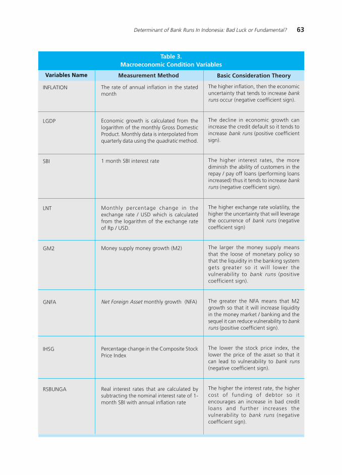
63Determinant of Bank Runs In Indonesia: Bad Luck or Fundamental?
Variables Name
Table 3.Macroeconomic Condition Variables
INFLATION
LGDP
SBI
LNT
GM2
GNFA
IHSG
RSBUNGA
Measurement Method Basic Consideration Theory
The higher inflation, then the economicuncertainty that tends to increase bankruns occur (negative coefficient sign).
The decline in economic growth canincrease the credit default so it tends toincrease bank runs (positive coefficientsign).
The higher interest rates, the morediminish the ability of customers in therepay / pay off loans (performing loansincreased) thus it tends to increase bankruns (negative coefficient sign).
The higher exchange rate volatility, thehigher the uncertainty that will leveragethe occurrence of bank runs (negativecoefficient sign)
The larger the money supply meansthat the loose of monetary policy sothat the liquidity in the banking systemgets greater so it wil l lower thevulnerability to bank runs (positivecoefficient sign).
The greater the NFA means that M2growth so that it will increase liquidityin the money market / banking and thesequel it can reduce vulnerability to bankruns (positive coefficient sign).
The lower the stock price index, thelower the price of the asset so that itcan lead to vulnerability to bank runs(negative coefficient sign).
The higher the interest rate, the highercost of funding of debtor so itencourages an increase in bad creditloans and further increases thevulnerability to bank runs (negativecoefficient sign).
The rate of annual inflation in the statedmonth
Economic growth is calculated from thelogarithm of the monthly Gross DomesticProduct. Monthly data is interpolated fromquarterly data using the quadratic method.
1 month SBI interest rate
Monthly percentage change in theexchange rate / USD which is calculatedfrom the logarithm of the exchange rateof Rp / USD.
Money supply money growth (M2)
Net Foreign Asset monthly growth (NFA)
Percentage change in the Composite StockPrice Index
Real interest rates that are calculated bysubtracting the nominal interest rate of 1-month SBI with annual inflation rate
64 Bulletin of Monetary, Economics and Banking, July 2011
Meanwhile, macroeconomic indicator (Fhit) includes inflation, economic growth, (LPDB),
1 month SBI interest rate, exchange rate (LNT), money supply growth (GM2), net foreign asset
growth (GNFA), stock exchange price index (IHSG), real interest rate (RSBUNGA) as described
below in Table 3. GDP quarterly data is interpolated to monthly.
V. RESULT AND ANALYSIS
5.1. Aggregately Bank runs Determinants (1990 √ 2005)
To estimate bank runs, we use Equation 1 and add dummy bank runs (dcrisis) on the
banking crisis occurred in 1997/1998.
This dummy variable addition is necessary to capture the occurrence of structural break
on the data, which may lead to the inefficient estimation result. As previously explained, following
D»Amato, Grubisic and Powell (1995) and McCandless, Gabrielli and Rouillet (2003), the
percentage change in a positive third-party funds means no bank runs occur, otherwise the
percentage change in third party funds that the negative means bank runs occur, where the
severity depends on the number of third-party withdrawals.
Since the model used is the GMM, the model robustness is analyzed by looking at the
moment condition. Arrelano and Bond (1991) suggested to use the serial correlation test of
Arrelano and Bond and Sargan as described in session 4. Based on the results of Arrelano-Bond
dynamic panel with one-step approach, there is a problem in a dynamic panel model (model 1),
i.e. there are problems with the auto correlation and over-identification in the variables used.
Considering this, the financial performance and macroeconomic indicators that exhibit
multicollinearity will not be used to avoid problems of specification inaccuracies and serial
correlation in the model. At the bank»s financial performance indicators, the ROE is not used
since we already have ROA. In addition, two variables have a close relationship so that it can
cause problems of multicollinearity. Likewise the credit growth variable (gkredit) is removed
because it is still associated with the loan to deposit ratio (LDR). For variable macroeconomic
indicators, the monthly growth of net foreign assets (GNFA) is not used because GNFA is a
factor affecting the growth of money supply (GM2). Besides, variable inflation, one-month
nominal interest rates of SBI, and real interest rates (RSBUNGA) will be separated with a distinctive
model. The separation is intended to avoid the relationship between interest rates with inflation
(2)
65Determinant of Bank Runs In Indonesia: Bad Luck or Fundamental?
that are interrelated. Taking into account the problems of multicollinearity, the model 1 is not
used to analyze the determinants of bank runs, but model 2 (model 1 with SBI minus ROE,
GKREDIT, GNFA, Inflation and rsbunga), model 3 (model 1 with INFLATION minus ROE, GKREDIT,
GNFA, SBI and rsbunga) and model 4 (model 1 with RSBUNGA minus ROE, GKREDIT, GNFA, SBI
and inflation).
The results of one-step model of 2, 3 and 4 are not robust based on Arrelano-Bond serial
correlation test, and Sargan tests indicated an over-identifying restriction problem. To overcome
these problems, we performe two-step regression of the Arrelano-Bond dynamic panel model.
This time, the two-step estimation results indicate that the model was robust. Furthermore the
F statistic of the three models was statistically significant at α = 1%, which means the model
can reject Ho: all independent variable coefficients are equal to zero. Thus, all independent
variables together influence the bank runs significantly. The results is presented in Table 4.
Sign of coefficient of the lag third-party funds (GDPK (-1)) is positive as expected. This
means decrease in third party funds in the previous period will lead to lower third-party funds
in the current period. The coefficient parameters (GDPK (-1)) in model 2, 3 and 4 are all significant,
as reflected by the p-value = 0.000. This significant coefficient indicates that the information
about bank runs can encourage the customers to withdraw their funds and can further lead to
the occurrence of bank runs on the other banks. The results are consistent D»Amato, Grubisic
and Powell (1995) and McCandless, Gabrielli and Rouillet (2003) which shows that self-fulfilling
prophecy factor is one of the causes of bank runs in Argentina in 1995 and 2001.
The results of the determinants of bank runs coming from the financial performance of
banks in the form of ROA, LDR, liq, NPL, and CA can be described as follows. The coefficient of
ROA has a positive sign so it accords to theoretical considerations as described in Table 2 and
Table 3, i.e. the higher the profitability of the bank, the better the financial performance of
banks so that it reduces vulnerability of the bank to bank runs. Concerning from its significance,
the p-value of ROA coefficient by 0.000, which means at α = 1% ROA significantly affects the
bank runs which is in this case it used a proxy variable used of bank runs is the change in bank
third party fund (GDPK).
LDR financial performance indicators show positive signs so it is not aligned as expected.
The LDR coefficient sign should have been negative because the higher the ratio the lower the
LDR liquidity available in the bank so the bank would be vulnerable to a massive withdrawal of
funds (bank runs). However, the LDR coefficient which is statistically significant affects the
bank run by the p-value 0.0000. The coefficient of LIQ also has a negative sign so it does not fit
with the expected sign, but it is statistically and significantly affects the bank runs. The explanation
66 Bulletin of Monetary, Economics and Banking, July 2011
of the opposite sign of the coefficient of two variables is mainly due to problems of limited
information from the customers in terms of the performance of banks (asymmetric information).
With limited information, the bank»s customers pay more attention to rates of return than the
publication of financial statements of banks in their fund withdrawals decision, as reflected by
compatibility of ROA coefficient. While the LDR and LIQ variable are not sensitive to the
withdrawal of third party funds.
Other financial performance indicators, the NPL showed a negative sign so that it fits
with the expected sign. Considering from its significance, it is statistically significant affecting
the bank run by the p-value of 0.000. Coefficient CA (capital adequacy ratio) has a negative
sign so it does not fit with the expected sign, but is statistically significant. As explained in the
LDR and LIQ, opposite sign of the coefficient is due to the limited information on the financial
statements of bank customers through publication so that changes in third party funds are not
sensitive to the capital adequacy ratio (CA). The significant variables of financial performance
show the healthier a finance of a bank, the less of the tendency of bunk runs.
The results of the determinant variables include macroeconomic conditions that include
LGDP, LNT, GM2, JCI, SBI, INFLATION and RSBUNGA will be described hereinafter. In all models,
economic growth (LGDP) has a positive sign so that it aligned as expected and is statistically
significant influencing bank runs on α = 1%. The exchange rate did not significantly affect the
bank run on all models. In model 2, the change in joint-stock index (IHSG) significantly affects
the bank run at α = 5%, but is not significant in models 3 and 4. Furthermore, IHSG and LNT
independent variable are separated by entering each variable in model 2, 3 and 4. Separation
was performed to detect the occurrence of multicollinearity between IHSG and LNT. The results
of dynamic panel with the separation of the two independent variables showed similar results,
i.e. IHSG remained significant and influence bank runs on the model 2 and has a negative sign
and did not significantly affect the bank runs in model 3 and 4. IHSG coefficient sign is negative
so that it is contrary to that expected. IHSG negative sign indicates that the placement of
customer funds in a bank is a substitution with the placement of funds in the stock market.
Other macroeconomic indicators that significantly affect the growth of bank runs are the money
supply M2 (GM2) with p-value of 0.000 in all three models.
SBI variables, INFLATION and RSBUNGA are estimated with separate models to avoid
multicollinearity problems. SBI using model 2, INFLATION with model 3, and RSBUNGA model
4. SBI coefficient on the model 2 is negative so that it aligned as expected and significantly
affects the bank run on α = 1%. Negative coefficient indicates the higher interest rates, the
greater the cost of funding of debtor so it encourages an increase in bad credit loans and
further increase the vulnerability to bank runs. INFLATION coefficient in model 3, did not
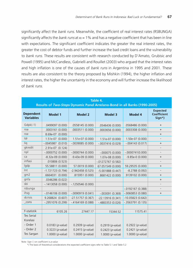
67Determinant of Bank Runs In Indonesia: Bad Luck or Fundamental?
significantly affect the bank runs. Meanwhile, the coefficient of real interest rates (RSBUNGA)
significantly affects the bank runs at α = 1% and has a negative coefficient that has been in line
with expectations. The significant coefficient indicates the greater the real interest rates, the
greater the cost of debtor funds and further increase the bad credit loans and the vulnerability
to bank runs. These results are consistent with research conducted by D»Amato, Grubisic and
Powell (1995) and McCandless, Gabrielli and Rouillet (2003) who argued that the interest rates
and high inflation is one of the causes of bank runs in Argentina in 1995 and 2001. These
results are also consistent to the theory proposed by Mishkin (1994), the higher inflation and
interest rates, the higher the uncertainty in the economy and will further increase the likelihood
of bank runs.
DependentVariables
Table 4.Results of Two-Steps Dynamic Panel Arrelano-Bond in all Banks (1990-2005)
Gdpk(-1)
roa
roe
ldr
liq
gkredit
npl
ca
inflasi
lgdp
lnt
gm2
gnfa
sbi
rsbunga
ihsg
dcrisis
_cons
F-statistik
Tes Serial
Korelasi
- Order 1
- Order 2
Tes Sargan
Model 1 Model 4Model 3Model 2Expected
CoefficientSign*)
.0499097 (0.000)
.0003161 (0.000)
8.69e-07 (0.000)
1.51e-07 (0.000)
-.0045987 (0.010)
2.91e-07 (0.124)
-.0000752 (0.000)
-8.32e-09 (0.000)
.010806 (0.523)
55.58811 (0.000)
-1.721723 (0.794)
.6664031 (0.000)
.0346286 (0.022)
-.1413058 (0.000)
-.0146106 (0.000)
9.268824 (0.607)
-.2951076 (0.299)
6105.26
0.0183 (p-value)
0.3223 (p-value)
1.0000 (p-value)
.0558145 (0.000)
.0003511 (0.000)
1.51e-07 (0.000)
-.0039085 (0.000)
-.0000744 (0.000)
-9.43e-09 (0.000)
57.0019 (0.000)
-2.942458 (0.525)
.815951 (0.000)
-.1250546 (0.000)
-.0090919 (0.041)
-27.51757 (0.367)
-.4164169 (0.088)
27447.17
0.2939 (p-value)
0.2415 (p-value)
1.0000 (p-value)
.0546436 (0.000)
.0003656 (0.000)
1.51e-07 (0.000)
-.0037416 (0.029)
-.000075 (0.000)
1.07e-08 (0.000)
-.01272767 (0.582)
67.051549 (0.000)
-5.001888 (0.447)
.8681422 (0.000)
-.003091 (0.369)
-22.13916 (0.341)
-.4883353 (0.026)
15344.52
0.2919 (p-value)
0.2423 (p-value)
1.0000 (p-value)
.0568486 (0.000)
.0003308 (0.000)
1.50e-07 (0.000)
-.004143 (0.017)
-.0000741(0.000)
-9.85e-0 (0.000)
59.29535 (0.000)
-8.2788 (0.092)
.9139102 (0.000)
-.0192167 (0.388)
-.0060853 (0.080)
-10.05823 (0.642)
-.3563791 (0.135)
11575.41
0.2922 (p-value)
0.2421 (p-value)
1.0000 (p-value)
+
+
+
-
+
-
-
+
-
+
-
+
+
-
-
+
Note: Sign ( ) on coefficient is p-value *) The basis of theoretical considerations the expected coefficient signs refer to Table 5.1 and Table 5.2
68 Bulletin of Monetary, Economics and Banking, July 2011
Meanwhile, the dummy banking crisis 1997-1998 (dcrisis) indicates the coefficients did
not significantly affect the dependent variable (bank runs) on all models. These results indicate
that there is no problem of structural breaks in the data of change percentage in third party
funds so without using a dummy crisis, estimation of bank runs determinant model in this
dissertation has been quite robust.
5.2. Bank runs Determinants in the period of Banking Crisis in 1997-1998
Bank runs determinants obtained from the result of data panel regression above by using
monthly data from 1990 until 2005. However, as known in 1997 until the year 1998 there was
bank runs in Indonesia that has sparked a national banking crisis. In this regard, this research
would also like to see the determinants of bank runs from January 1997 until December 199811.
In addition, the analysis of bank runs determinants in the period 1997-1998 is a control variable
to use the change of third party funds as a proxy of bank runs. As explained in section 4, the
control variable is necessary given the changes of third party funds are not always followed by
the occurrence of bank runs.
In relation to have multicollinearity between independent variables, then to analyze the
bank runs determinants on the period of banking crisis in 1997-1998 used models 2, 3 and 4.
The estimation of Arrelano-Bond dynamic data panel model with one-step approach shows
bias result because the results of regression indicate the presence of serial correlation problem
and over-identifying problem in restriction equation. In connection with the problems, looked
for models that are not biased (robust), using two-step model of Arrelano-Bond dynamic panel,
the results can be seen in Table 5. GMM regression results show that the relationship between
the dependent variable with independent variable are statistically significant, as reflected by
the F values statistically significant at α = 1%.
Based on the results of GMM regressions, the three models showed a lag DPK are used
as a proxy of self-fulfilling prophecy has a positive sign and statistically significant with a p-
value of 0.000 or α less than 1%. The significant coefficient shows that the news of a reduction
in funds or bank run in another bank can cause to other customers in droves attracted funds in
the bank (bank runs). The results of study are in line with bank runs research in Argentina
conducted by D»Amato, Grubisic and Powell (1995) and McCandless, Gabrielli and Rouillet
11 Massive funds withdrawals has been experienced since Government change the policy from managed floating exchange rate tofreely freely floating exchange rate on 14 August 1997 and the wave of bank runs was getting bigger since the closure of 16 bankson November 1997 until it gets recovered on August 1998
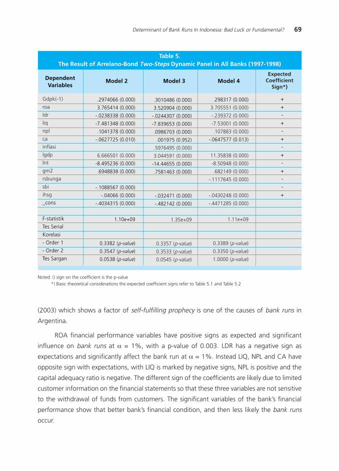
69Determinant of Bank Runs In Indonesia: Bad Luck or Fundamental?
(2003) which shows a factor of self-fulfilling prophecy is one of the causes of bank runs in
Argentina.
ROA financial performance variables have positive signs as expected and significant
influence on bank runs at α = 1%, with a p-value of 0.003. LDR has a negative sign as
expectations and significantly affect the bank run at α = 1%. Instead LIQ, NPL and CA have
opposite sign with expectations, with LIQ is marked by negative signs, NPL is positive and the
capital adequacy ratio is negative. The different sign of the coefficients are likely due to limited
customer information on the financial statements so that these three variables are not sensitive
to the withdrawal of funds from customers. The significant variables of the bank»s financial
performance show that better bank»s financial condition, and then less likely the bank runs
occur.
DependentVariables
Table 5.The Result of Arrelano-Bond Two-Steps Dynamic Panel in All Banks (1997-1998)
Gdpk(-1)
roa
ldr
liq
npl
ca
inflasi
lgdp
lnt
gm2
rsbunga
sbi
ihsg
_cons
F-statistik
Tes Serial
Korelasi
- Order 1
- Order 2
Tes Sargan
Model 4Model 3Model 2Expected
CoefficientSign*)
.2974066 (0.000)
3.765414 (0.000)
-.0238338 (0.000)
-7.481348 (0.000)
.1041378 (0.000)
-.0627725 (0.010)
6.666501 (0.000)
-8.495236 (0.000)
.6948838 (0.000)
-.1088567 (0.000)
-.04066 (0.000)
-.4034315 (0.000)
1.10e+09
0.3382 (p-value)
0.3547 (p-value)
0.0538 (p-value)
.3010486 (0.000)
3.520904 (0.000)
-.0244307 (0.000)
-7.839653 (0.000)
.0986703 (0.000)
.001975 (0.952)
.5976495 (0.000)
3.044591 (0.000)
-14.44655 (0.000)
.7581463 (0.000)
-.032471 (0.000)
-.482142 (0.000)
1.35e+09
0.3357 (p-value)
0.3533 (p-value)
0.0545 (p-value)
.298317 (0.000)
3.705551 (0.000)
-.239372 (0.000)
-7.53001 (0.000)
.107883 (0.000)
-.0647577 (0.013)
11.35838 (0.000)
-8.50948 (0.000)
.682149 (0.000)
-.1117645 (0.000)
-.0430248 (0.000)
-.4471285 (0.000)
1.11e+09
0.3389 (p-value)
0.3350 (p-value)
1.0000 (p-value)
+
+
-
+
-
+
-
+
-
+
-
-
+
Noted: () sign on the coefficient is the p-value *) Basic theoretical considerations the expected coefficient signs refer to Table 5.1 and Table 5.2
70 Bulletin of Monetary, Economics and Banking, July 2011
The variable of macroeconomic indicator, in the form of economic growth (LGDP), the
exchange rate (LNT) and the money supply growth (M2) in all three models have signs as
expected and significantly affect the bank run at α = 1%. The significant coefficient of LGDP
shows that better economic growth, the less likely bank runs. While LNT significant coefficient
shows the higher the depreciation of exchange rate, then higher bank foreign liabilities
denominated in rupiahs and will further increase the likely bank runs. GM2 significant coefficient
shows increasing the money supply, then greater the liquidity available at banking and will
further reduce the possibility of bank runs. The results are consistent with the results of research
conducted by Demirguc-Kunt and Detragiache (1998), Hardy and Pazarbasiouglu (1999) and
Ho (2004) which showed economic growth and exchange rates affect bank runs and banking
crisis.
Other significant macroeconomic variables affect the bank runs at α = 1% and has a sign
in accordance with the theory of bank runs is a 1-month SBI in model 2, Inflation in models 3
and real interest rates (RSBUNGA) in model 4. The significant of inflation coefficient, SBI interest
rates and real interest are consistent with the theories argued by Mishkin (1994) and D»Amato
research, Grubisic and Powell (1995) and McCandless, Gabrielli and Rouillet (2003) who argued
that the interest rates and high inflation is one of the causes of bank runs.
Meanwhile, the IHSG variable on all three significant models affect bank runs at α = 1%,
but the coefficient is negative that is inconsistent with the theory as described in Table 2 and
Table 3. The negative of IHSG coefficient shows that the third party funds in banking is a
substitute for the stock product.
VI. CONCLUSION
This paper provide the empirical test of bank runs determinants in Indonesia. Focusing
on the self-fulfilling prophecy, the dynamic panel result shows that the self-fulfilling prophecy
variable significantly influences the bank runs in Indonesia. The implication policy from this
result shows that the information of bank runs occurrence or the third party significant withdrawal
in a bank can influence the customer»s expectation to greatly withdraw money in other bank.
Regarding to the discovery, in the bank risk based supervision frame, supervisor authority needs
to map the sensitive banks toward self-fulfilling prophecy factor. The bank sensitivity mapping,
is inserted to the cycle of bank supervision in risk valuation frame toward bank individual so
that can be early prevented the contagious bank runs impact from one bank to another bank.
Besides, reliable communication management needs to be built to restore the worsen society»s
expectation toward a bank. Building customer trust toward bank needs also to be supported
71Determinant of Bank Runs In Indonesia: Bad Luck or Fundamental?
by government as the source of emergency funding in terms of bank runs occurrence that has
systemic risk. Support can be done by increasing the coordination on bank supervision, between
Bank Indonesia with government via existing financial system stability forum.
Caveat
This research is using lag of independent variable (third party fund change percentage) as
bank runs proxy. The use of this robust variable to get the self-fulfilling prophecy factor, however,
it is still possible to find better proxy.
72 Bulletin of Monetary, Economics and Banking, July 2011
REFERENCES
Aharony, Joseph, and Itzhak Swary. ≈Contagion Effects of Bank Failures: Evidence from Capital
Markets.∆ The Journal of Business, July 1983, 56(3), pp. 305-322.
Allen, Franklin, and Douglas Gale. ≈Optimal Financial Crises∆ The Journal of Finance, Vol. 53,
No.4, Papers and Proceedings of the Fifty-Eighth Annual Meeting of the American Finance
Association, Chicago, Illinois, January 3-5, 1998 (Aug., 1998), pp. 1245-1284.
______. ≈Bubbles and Crises∆. The Economic Journal, Vol. 110, No. 460 (Jan., 2000), hal. 236-
255.
______. ≈Financial Contagion.∆ The Journal of Political Economy, February 2000, 108(1), pp. 1-
33.
Bank Indonesia, Annual Report of Bank Indonesia from 1997/1998 until 2007.
Bryant, John.
≈Bank Collapse and Depression∆ Journal of Money, Credit and Banking, Vol. 13, No. 4 (Nov.,
1981), pp. 454-464.
Calomiris, Charles W. ≈Bank Failures in Theory and History: The Great Depression and Other
«Contagious» Events.∆ NBER Working Paper Series, No. WP 13597, November 2007.
______, dan Gary Gorton.∆≈The Origins of Banking Panics: Models, Facts, and Bank Regulation∆.
Dalam R. G. Hubbard, Financial markets and Financial Crisis. Chicago: University of Chicago
Press, hal. 109-173, 1991.
Canova, Fabio. ≈Were Financial Crises Predictable?∆ Journal of Money, Credit, and Banking,
Vol. 26, 1 (Februari 1994), hal. 102-124.
D»Amato, Laura, Elena Grubisic dan Andrew Powell, 1997, ≈Contagion, Bank Fundamentals or
Macroeconomic Shock? An Empirical Analysis of the Argentine 1995 Banking Problems∆,
1997, Banco Central de la República Argentina Working Paper Number 2, July 1997.
Davis, E. Philip dan Dilruba Karim. ≈Comparing Early Warning Systems for Banking Crises.∆
Working Paper Brunel University dan NIESR West London, 2007.
Demirguc-Kunt, Asli dan Detragiache, Enrica.
≈The Determinants of Banking Crises: Evidence from Developing and Developed Countries.∆
IMF Working Paper, No. WP/97/106, September 1997.
73Determinant of Bank Runs In Indonesia: Bad Luck or Fundamental?
Diamond, Douglas W. ≈Debt Maturity Structure and Liquidity Risk.∆ The Quaterly Journal of
Economics, August 1991, 106(3), pp. 709-737.
______, dan Philip H. Dybvig, ≈Bank Runs, Deposit Insurance, and Liquidity.∆ Journal of Political
Economy, June 1983, 91(3), hal. 401-419.
Kaufman, George G. ≈Bank Runs: Causes, Benefits and Costs.∆ Cato Journal 2, no. 3 (Winter
1988): 559-88.
______. ≈The Concise Encyclopedia of Economics di website≈http://www.econlib.org/library/
Enc/BankRuns.html∆ mimeo.
Kindleberger, C. P. Manias, Panics and Crashes. Basic Books, New York, 1978.
Lindgren, Carl-Johan; Garcia, Gillian, Garcia; dan Saal, Matthew I.∆Bank Soundness and
Macroeconomic Policy.∆ IMF, 1996.
McCandless, George, Maria F. Gabrielli, Maria J. Rouillet, 2003, ≈Determining the Causes of
Bank Runs in Argentina During the Crisis of 2001∆, Revista De Analisis Economico, Vol. 18,
No. 1, Banco Central de la República Argentina.
Minsky, Hyman. ≈A Theory≈of System Fragility∆, dalam Edward Altman dan Arnold Sametz
(ed.), Financial Crises: Institutions and Markets in a Fragile Financial Environment, New York:
Wiley-Interscience, 1977.
Mishkin, Frederic S.
≈Understanding Financial Crises: A Developing Country Perspective.∆ NBER Working Paper
Series, No. WP 5600, Mei 1996.
Safuan, Sugiharso. ≈Contagion and Interdependence in the Asian Crisis∆. Proceedings Seminar
Pusat Pendidikan dan Studi Kebanksentralan, Bank Indonesia. Jakarta, 27 Agustus 2003.
Warjiyo, Perry. ≈Bank Failure Management: The Case of Indonesia∆ APEC Policy Dialogue on
Bank Failure Management Paper, Mexico, June 7-8, 2001.

74 Bulletin of Monetary, Economics and Banking, July 2011
This page is intentionally left blank
75Long-Run Money and Inflation Neutrality Test in Indonesia
LONG-RUN MONEY AND INFLATION NEUTRALITY TESTIN INDONESIA
Arintoko 1
This paper investigates long-run neutrality of money and inflation in Indonesia, with due consideration
to the order of integration, exogeneity, and cointegration of the money stock-real output and the money
stock-price, using annual time-series data. The Fisher-Seater methodology is used to do the task in this
research. The empirical results indicate that evidence rejected the long-run neutrality of money (both
defined as M1 and M2) with respect to real GDP, showing that it is inconsistent with the classical and
neoclassical economics. However, the positive link between the money and price in long run holds for
money defined as M1 rather than M2, which consistent with these theories. In particular, besides the
positive effect to long-run inflation, monetary expansions have long-run positive effect on real output in
the Indonesian economy.
1 Lecturer Staff of Faculty of Economic of Jenderal Soedirman University, and a PHD student at Postgraduate Program of EconomicScience, UGM. e-mail: [email protected].
Abstract
JEL: C32, E31, E51
Keywords: long-run neutrality of money, inflation, unit root, exogeneity, cointegration
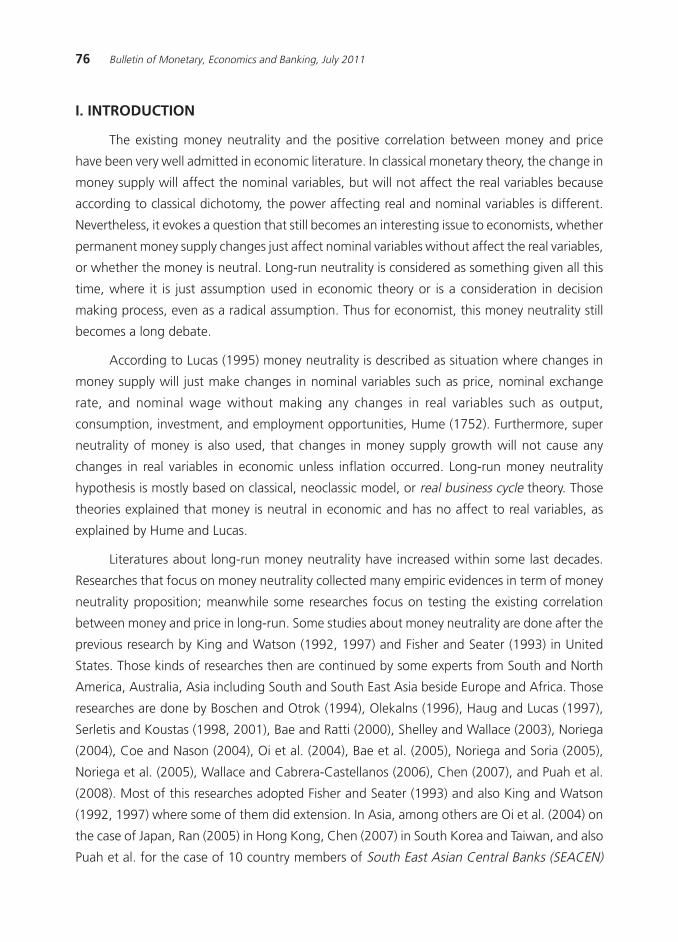
76 Bulletin of Monetary, Economics and Banking, July 2011
I. INTRODUCTION
The existing money neutrality and the positive correlation between money and price
have been very well admitted in economic literature. In classical monetary theory, the change in
money supply will affect the nominal variables, but will not affect the real variables because
according to classical dichotomy, the power affecting real and nominal variables is different.
Nevertheless, it evokes a question that still becomes an interesting issue to economists, whether
permanent money supply changes just affect nominal variables without affect the real variables,
or whether the money is neutral. Long-run neutrality is considered as something given all this
time, where it is just assumption used in economic theory or is a consideration in decision
making process, even as a radical assumption. Thus for economist, this money neutrality still
becomes a long debate.
According to Lucas (1995) money neutrality is described as situation where changes in
money supply will just make changes in nominal variables such as price, nominal exchange
rate, and nominal wage without making any changes in real variables such as output,
consumption, investment, and employment opportunities, Hume (1752). Furthermore, super
neutrality of money is also used, that changes in money supply growth will not cause any
changes in real variables in economic unless inflation occurred. Long-run money neutrality
hypothesis is mostly based on classical, neoclassic model, or real business cycle theory. Those
theories explained that money is neutral in economic and has no affect to real variables, as
explained by Hume and Lucas.
Literatures about long-run money neutrality have increased within some last decades.
Researches that focus on money neutrality collected many empiric evidences in term of money
neutrality proposition; meanwhile some researches focus on testing the existing correlation
between money and price in long-run. Some studies about money neutrality are done after the
previous research by King and Watson (1992, 1997) and Fisher and Seater (1993) in United
States. Those kinds of researches then are continued by some experts from South and North
America, Australia, Asia including South and South East Asia beside Europe and Africa. Those
researches are done by Boschen and Otrok (1994), Olekalns (1996), Haug and Lucas (1997),
Serletis and Koustas (1998, 2001), Bae and Ratti (2000), Shelley and Wallace (2003), Noriega
(2004), Coe and Nason (2004), Oi et al. (2004), Bae et al. (2005), Noriega and Soria (2005),
Noriega et al. (2005), Wallace and Cabrera-Castellanos (2006), Chen (2007), and Puah et al.
(2008). Most of this researches adopted Fisher and Seater (1993) and also King and Watson
(1992, 1997) where some of them did extension. In Asia, among others are Oi et al. (2004) on
the case of Japan, Ran (2005) in Hong Kong, Chen (2007) in South Korea and Taiwan, and also
Puah et al. for the case of 10 country members of South East Asian Central Banks (SEACEN)
77Long-Run Money and Inflation Neutrality Test in Indonesia
Research and Training Centre. Meanwhile the issue of the existing positive correlation between
money and price were collected in the latest studies by Saatcioglu and Korap (2009), Roffia and
Zaghini (2007), also Browne and Cronin (2007). The result conform the conclusions from previous
researchers such as Lucas (1980), Dwyer and Hafer (1988), Friedman (1992), Barro (1993),
McCandless and Weber (1995), Rolnick and Weber (1997), Dewald (1998), Dwyer (1998),
Dwyer and Hafer (1999).
The studies in some cases found supporting evidences about the existing money neutrality,
but not the money super neutrality. On the long run correlation between money and price,
empirical result generally gives the same conclusion about the existence of positive correlation
between money and price; even there are some differences in terms of time-series characteristics
from data obtained in some countries.
The paper will test the preposition of long-run money neutrality using either M1 or M2
towards real output and price in Indonesia. This research uses annual time series data. Research
focusing on this issue is expected to enrich economic literature and studies and also becomes
deep consideration for monetary policy maker.
This paper is started with introduction that contains why the research in terms of long-
run inflation and money neutrality test is very important for Indonesian. The second part of this
paper discusses and reviews the previous research. The third part explains research method
about Fisher-Seater methodology including its prerequisites test such as integration, exogeneity,
and cointegration. The forth part provides the result of the research and explanation that will
be ended by the fifth part as a conclusion and suggestion.
II. THEORY
2.1. Hume View and Classical Quantitative Theory
According to money quantitative theory, Hume emphasized the unit change of money
stock and its irrelevance towards rational society»s behavior. He stated that money is meaningless;
however money represents labor and commodity.
There are two Hume»s statements that formed a doctrine that a change in money supply
stock will have an effect on proportional change towards all prices that reflected in a currency
unit and has no effect on real variables like how many people work and how many products
manufactured and consumed. Prediction from quantitative theory is that in the long-run the
growth money supply is neutral towards the number production growth and influences the
inflation proportionally. In a quantity equation from classical quantity theory,
78 Bulletin of Monetary, Economics and Banking, July 2011
(1)
(6)
Where the equation relates money quantity (M) towards nominal output (P x Y), meanwhile V
shows the velocity of money. The quantity equation shows that the increase of money quantity
reflects one of the three other variables, either price increase, output increase, or money velocity
decrease, though this velocity tends to be stable all the time. When Central Bank changes
money supply, it will cause a proportional change on nominal output (P x Y). Because money
is neutral according to classical theory, money does not influence the real output, Y, but do
change the price, P.
2.2. Neoclassical Model
Theoretical explanation in classical model below is mostly adopted from Barro (1997).
This model is started with small opened economic model with four equations assuming the
existence of perfect capital mobility assumption.
(2)
(5)
(4)
(3)
There are four unknown parameters in real output model y, real interest rate r, real
exchange rate ε, and price P. Equation (2) shows equilibrium for goods market in which its
demand, E is the function from real income, real interest rate, and real exchange rate. Real
exchange rate in this definition is:
where e is nominal exchange rate, P and Pf are domestic and foreign price rate respectively.
The increase in ε represents the appreciation of domestic currency that decreases net real
export and decreases real goods demand.
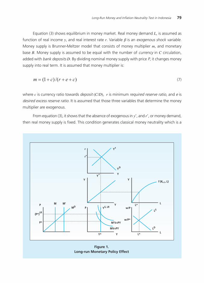
79Long-Run Money and Inflation Neutrality Test in Indonesia
Equation (3) shows equilibrium in money market. Real money demand L, is assumed as
function of real income y, and real interest rate r. Variable β is an exogenous shock variable.
Money supply is Brunner-Meltzer model that consists of money multiplier m, and monetary
base B. Money supply is assumed to be equal with the number of currency in C circulation,
added with bank deposits D. By dividing nominal money supply with price P, it changes money
supply into real term. It is assumed that money multiplier is:
where c is currency ratio towards deposit (C/D), r is minimum required reserve ratio, and e is
desired excess reserve ratio. It is assumed that those three variables that determine the money
multiplier are exogenous.
From equation (3), it shows that the absence of exogenous in y*, and r*, or money demand,
then real money supply is fixed. This condition generates classical money neutrality which is a
(7)
Figure 1.Long-run Monetary Policy Effect
r Ys
r*
YD
YY*
Y Yf (Kt-1, L)
P
(P*)LR
P*
M M»MD P
YYS, LR
Y* Y
M»V=PY
MV=PY
w/P*
w/PL* L
LS
LD
LL*
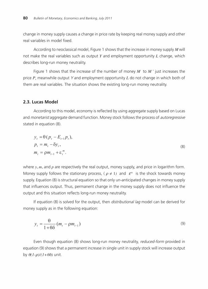
80 Bulletin of Monetary, Economics and Banking, July 2011
(8)
change in money supply causes a change in price rate by keeping real money supply and other
real variables in model fixed.
According to neoclassical model, Figure 1 shows that the increase in money supply M will
not make the real variables such as output Y and employment opportunity L change, which
describes long-run money neutrality.
Figure 1 shows that the increase of the number of money M to M « just increases the
price P, meanwhile output Y and employment opportunity L do not change in which both of
them are real variables. The situation shows the existing long-run money neutrality.
2.3. Lucas Model
According to this model, economy is reflected by using aggregate supply based on Lucas
and monetarist aggregate demand function. Money stock follows the process of autoregressive
stated in equation (8).
where y, m, and p are respectively the real output, money supply, and price in logarithm form.
Money supply follows the stationary process, ( ρ = 1) and εm is the shock towards money
supply. Equation (8) is structural equation so that only un-anticipated changes in money supply
that influences output. Thus, permanent change in the money supply does not influence the
output and this situation reflects long-run money neutrality.
If equation (8) is solved for the output, then distributional lag model can be derived for
money supply as in the following equation:
(9)
Even though equation (8) shows long-run money neutrality, reduced-form provided in
equation (9) shows that a permanent increase in single unit in supply stock will increase output
by θ(1-ρ)/(1+θδ) unit.
81Long-Run Money and Inflation Neutrality Test in Indonesia
2.4. The Previous Research
Some empirical evidences on money neutrality are study by McCandless and Weber (1995),
who found a high correlation (more than 0,9) between inflation and the growth of money
supply using indicator M0, M1, even M2 along 30 years in 110 countries. Instead, McCandless
and Weber found the absence of correlation between the growth of money supply and the
growth of real output within the same period. Meanwhile Shelley and Wallace (2003) tested
the long-run money neutrality and found the money neutrality within 1932-1981 periods in
Mexico. However, in 1932-2001, Shelley and Wallace using the model developed by Fisher and
Seater found that there was no money neutrality regardless the size definition of money supply
used. Wallace and Cabrera-Castellanos (2006) who also refer to Fisher-Seater model found the
existing money neutrality in Guatemala during 1950-2002. This study found the existing M1
neutrality with GDP, expenditure, and consumption.
By using Fisher and Seater methodology, Bae and Ratti (2000) tested the existing long-
run neutrality and super neutrality in Argentina and Brazil. Using low frequency data for money
supply and output, this study found evidence that supports the existing hypothesis of money
neutrality in Argentina and Brazil. However this research did not find the super neutrality evidence
in both countries.
Some researchers, Oi et al. (2004), Chen (2007), and Puah et al. (2008) found some
evidences of long-run monetary neutrality in Asian Countries. Oi et al. (2004), by using King
and Watson (1997) methodology, found the long-run monetary neutrality evidence in Japan
for variable M2 within 1890 √ 2003 period. With the same methodology, but with quarterly
data, Chen (2007) found evidence that long-run monetary neutrality M2 also occurs in South
Korea within 1970.1 √ 2004.4. Meanwhile Puah et al. (2008), by using Fisher-Seater methodology
found the long-run monetary neutrality evidence towards M1 in some Asian countries such as
Malaysia, Myanmar, Nepal, Philippine, and South Korea.
In contrast, some other researchers found different evidences which are non-neutrality
of money instead. Among others, Fisher and Seater (1993) shows that M2 is not neutral in US
during 1968 √ 1975, Shelley and Wallace (2003) during 1932 √ 2001 period in Mexico, and
Ran (2005) who tested the long-run money neutrality on two exchange rate regimes in Hong
Kong. Ran tested money neutrality based on Fisher and Seater model expansion (1993) and
found that M1 is not neutral under floating exchange rate regime. With the same methodology,
this empirical evidence was also found by Puah et al. (2008) that M1 is not neutral on the long-
run in Indonesia during 1965 √ 2002. Long-run non-neutrality evidence for M1 was also found
82 Bulletin of Monetary, Economics and Banking, July 2011
by Puah in Taiwan and Thailand respectively during 1951 √ 2002 and 1953 √ 2002. Long-run
monetary non-neutrality evidence in Taiwan was supported by Chen (2007) study using quarterly
M2 data referring the method of King and Watson (1997).
Meanwhile the existing issue in terms of positive correlation between money and price
was collected by, one of them, the latest study by Saatcioglu and Korap (2009) who tested
money and price correlation validity based on the quantity theory of money in Turkey. The
result shows that the empirical evidence supports the existing proportional relationship between
money and price in Turkey»s economy. Other study carried out by Roffia and Zaghini (2007)
who analyzed money growth towards inflation dynamic in 15 countries. Using 3 years horizon,
they found the positive correlation between aggregate monetary and price in about 50% of
the observed countries. Another study is Browne and Cronin (2007) who found an empirical
evidence that supports the existing correlation between price (both commodity and consumer
price) and money supply in the long-run in US. Empirical result from those latest researches
accorded the conclusion by Lucas (1980), Dwyer and Hafer (1988), Friedman (1992), Barro
(1993), McCandless and Weber (1995), Rolnick and Weber (1997), Dewald (1998), Dwyer
(1998), Dwyer and Hafer (1999), where the change of money supply has a tight correlation
with the price rate .
III. METHODOLOGY
3.1. Variables and Data
On econometric analysis, we use annual data covering 1970-2008 periods. The definitions
of money supply used are M1 and M2. The behavior of these two definitions of money (m) are
are important in terms of their influence on real macroeconomic variables such as output (y),
beside the nominal variable such as price (p). Real output is represented by real Gross Domestic
Product (GDP) with year 2000 constant price, meanwhile price is represented by Consumer
Price Index (CPI) with the same base year. Initial data was obtained from Indonesia Economic
and Financial Statistics (SEKI), Indonesia Banking Annual Report, and Indonesia Statistics, BPS
various years.
M1 is a narrow definition for money supply or money velocity. M1 includes fiat money
and giral money. M2 is a wide definition for money supply that includes M1 added by near
money, like savings deposit in commercial bank and time deposits. Thus fiat money added by
giral money is M1, and M1 added by quasy money is M2.
83Long-Run Money and Inflation Neutrality Test in Indonesia
3.2. Integrated Series and Exogeneity
Integrated series from variables included in Fisher-Seater methodology will determine an
appropriate test form. In this case, the data series of money, output, and price determine the
appropriate FS test form to test long-run neutrality of money and inflation.
FS model required that in long-run neutrality test, all variables are integrated in the same
order, which is assumed as I(1). In FS application , it is assumed that money, output, and price
are I(1). To test integrated of order from variables used, then this research conducted unit root
test through Augmented Dickey-Fuller (ADF) and Phillips-Perron (PP). ADF test is based on the
following autoregressive process or AR(1):
where µ and ρ are parameters, and εt is assumed as white noise. y is stationary series if -1 < r
< 1. Dickey-Fuller test (DF) and PP use root unit as null hypotheses, H0: ρ = 1 and H1: ρ < 1. The
test was done by estimating equation (10) and subtract with yt-1
in both side of the equation
would give:
(11)
(10)
H0: γ = 0; H
1: γ < 1
Meanwhile Phillips and Perron (1988) proposed a non-parametric method to control
high order serial correlation . PP test is a regression with AR(1) process:
where, ργ −= 1 and the null hypotheses and its alternative are:
(12)
When ADF test corrects high order serial correlation with the addition of lagged differenced
terms on the right side of the equation, PP test does a t-statistic correction of coefficient γ from
AR(1) regression to calculate serial correlation in ε.
84 Bulletin of Monetary, Economics and Banking, July 2011
(15)
where it is assumed that disturbances u1 and u
2 are not correlated. Based on equation (14),
money (m) is exogenous only if the estimation result accepts H0:δ
j = 0. The hypothesis
interprets that output and price variables (as variable y) in the model do not influence the
money (m).
Test result rejects H0 if F(m,n – z) statistic > F(m,n – z) critical value on α = 5%, with
degree of freedom m and n-z, where m = lag sum, n = number of observation, and z = the
number of estimated parameter. Causality test based on equation (13) and (14) for this exogeneity
test refers to Hafer (1982) as expressed by Gujarati and Porter 20092 that uses money growth
(m) and output growth (y).
3.3. Cointegration Test
Cointegration test is carried out to prove the existing of long-run correlation among the
estimated variables. Fisher and Seater (1993) argued that monetary neutrality would involve
the existence of permanent change in money supply. In this definition, according to Engle and
Granger (1987), the real and nominal variables need I(1); however both of them are not
cointegrated. Cointegration test in a multivariate system uses Johansen (1995) approach based
on the following formulation:
Furthermore, to apply FS methodology it has to fulfill the assumption that money
which is M1 and M2 are exogenous. M1 and M2 are is exogenous if the variables are not
influenced or caused by y variable in Granger causality test on the following bivariate
regression :
(13)
(14)
..
2 See Gujarati and Porter (2009) page 699
85Long-Run Money and Inflation Neutrality Test in Indonesia
(17)
(16)
(18)
where k = number of lag. In the hypothesis test it uses the following Likelihood Ratio (LR) test
statistic,
for r = 0, ,…., k-1 where λi is eigenvalue value. T is the size of sample. Q
r is also called trace
statistic. This test rejects H0 stating there is no cointegration if LR statistic > its critical value on
the chosen α.
3.4. Fisher-Seater Methodology
FS methodology was firstly introduced by Fisher and Seater (1993) by using bivariate
system to test long-run money neutrality, where money measurement is one of the variables.
Bivariate system used follows these two equations:
where, )(La , b(L), c(L) and d(L) are lag polynomial, while b0 and c
0 are not restricted. Error
vector (ut,w
t) ~ iid (0,Σ). In this methodology, it is assumed that x t = ∆im
t and z t = ∆ jm
t with
i,j = 0 or 1. The first variable is m, the nominal money supply M in natural logarithm. The
second variable is y expressing nominal and real variables in natural logarithm, like real output
and price. If m and y variables are not integrated on the level or I(0) then the two variables must
have the same integration order. say in first level or I(1). When variable m is I(1), then the
appropriate test is the long-run neutrality of money and inflation, and if variable m is I(2), then
the appropriate test is long-run super neutrality test.
Fisher and Seater defined long-run derivative (LRD) as a marginal in z towards permanent
change in x, which is written as follow:
(19)
where
86 Bulletin of Monetary, Economics and Banking, July 2011
(21)
(22)
3 See Fisher and Seater (1993) page 404.4 Barlett Estimator is infinite limit of the slope coefficient.
(20)
where α(L) and γ(L) are function from coefficient of equation (17) and (18) which are α(L)=d(L)/
[a(L)c(L)-b(L)c(L)] and γ(L)=c(L)/[a(L)c(L)-b(L)c(L)] 3
Referring to Fisher and Seater, money will be neutral in the long-run (LRN) if LRDy,m
= λ,
where λ = 1 if y is nominal variable, and λ = 0 if y is real one. Meanwhile the money will be
super neutral in the long run (long-run super neutrality, LRSN ) if LRDy, ∆m
= µ, where µ = 1 if y
is nominal variable, and µ = 0 if y is real one.
By assuming that money supply variable are exogenous and error term ut and w
t are not
correlated in ARIMA model, then c(1)/d(1) is Bartlett4 estimator from zero frequency in regression
∆(y)yt towards ∆(m)m
t. Estimation c(1)/d(1) is given with , where β
k is slope coefficient
from the following ordinary least squares (OLS) regression:
Equation (19) shows that long-run derivative is the limit of output elasticity towards
money. If the limit of denominator on the equation is zero, it means there is no permanent
change of monetary variable, so (m) = 0, hence we cannot do the neutrality test. For (m) > 1, FS
methodology shows that equation (19) can be re-written as follow:
when (m) = (y) = 1, long-run neutrality of money and inflation (LRN) can be tested and equation
(21) would be:
The null hypothesis tests for long-run neutrality of money and inflation are βk respectively
for y as output and price. If the result of estimation does not reject null hypothesis then the
preposition of long-run neutrality of money and inflation are empirically supported. In result
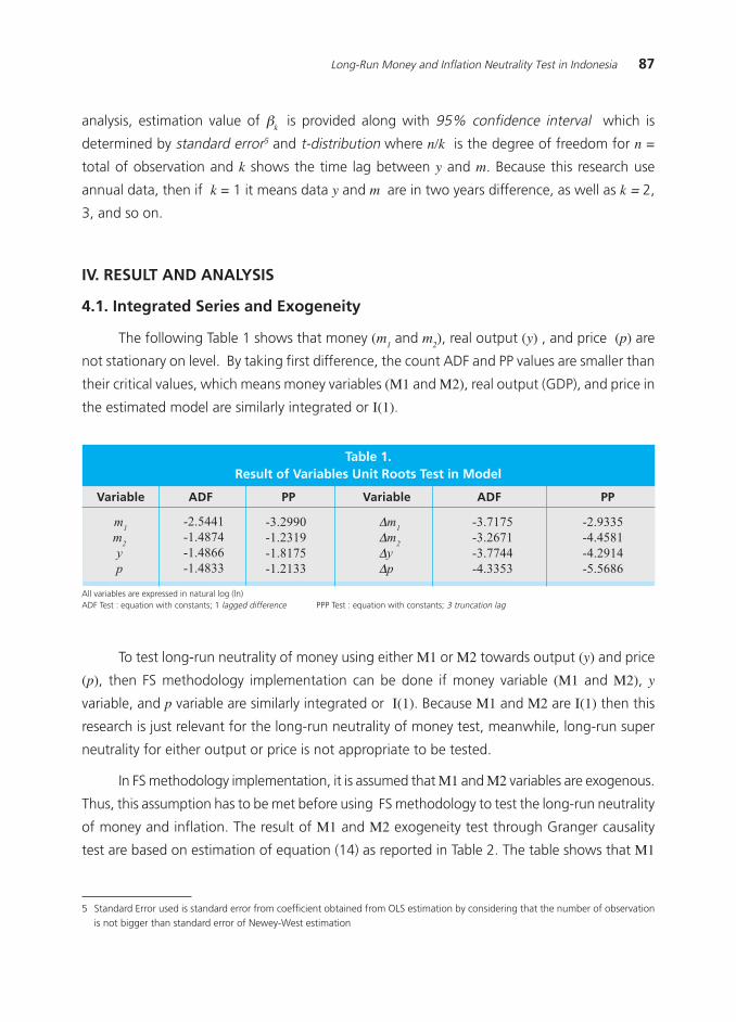
87Long-Run Money and Inflation Neutrality Test in Indonesia
analysis, estimation value of βk is provided along with 95% confidence interval which is
determined by standard error5 and t-distribution where n/k is the degree of freedom for n =
total of observation and k shows the time lag between y and m. Because this research use
annual data, then if k = 1 it means data y and m are in two years difference, as well as k = 2,
3, and so on.
IV. RESULT AND ANALYSIS
4.1. Integrated Series and Exogeneity
The following Table 1 shows that money (m1 and m
2), real output (y) , and price (p) are
not stationary on level. By taking first difference, the count ADF and PP values are smaller than
their critical values, which means money variables (M1 and M2), real output (GDP), and price in
the estimated model are similarly integrated or I(1).
5 Standard Error used is standard error from coefficient obtained from OLS estimation by considering that the number of observationis not bigger than standard error of Newey-West estimation
Table 1.Result of Variables Unit Roots Test in Model
-2.9335
-4.4581
-4.2914
-5.5686
Variable ADF PP Variable ADF PP
m1
m2
y
p
-2.5441
-1.4874
-1.4866
-1.4833
-3.2990
-1.2319
-1.8175
-1.2133
∆m1
∆m2
∆y
∆p
-3.7175
-3.2671
-3.7744
-4.3353
All variables are expressed in natural log (ln)ADF Test : equation with constants; 1 lagged difference PPP Test : equation with constants; 3 truncation lag
To test long-run neutrality of money using either M1 or M2 towards output (y) and price
(p), then FS methodology implementation can be done if money variable (M1 and M2), y
variable, and p variable are similarly integrated or I(1). Because M1 and M2 are I(1) then this
research is just relevant for the long-run neutrality of money test, meanwhile, long-run super
neutrality for either output or price is not appropriate to be tested.
In FS methodology implementation, it is assumed that M1 and M2 variables are exogenous.
Thus, this assumption has to be met before using FS methodology to test the long-run neutrality
of money and inflation. The result of M1 and M2 exogeneity test through Granger causality
test are based on estimation of equation (14) as reported in Table 2. The table shows that M1
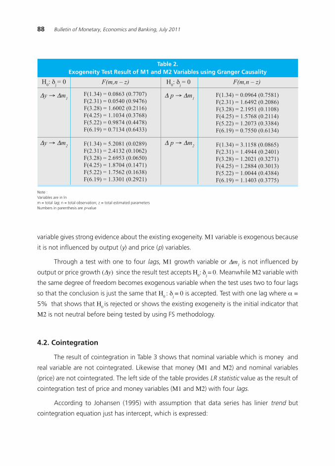
88 Bulletin of Monetary, Economics and Banking, July 2011
variable gives strong evidence about the existing exogeneity. M1 variable is exogenous because
it is not influenced by output (y) and price (p) variables.
Through a test with one to four lags, M1 growth variable or ∆m1 is not influenced by
output or price growth (∆y) since the result test accepts H0: δ
j = 0. Meanwhile M2 variable with
the same degree of freedom becomes exogenous variable when the test uses two to four lags
so that the conclusion is just the same that H0 : δ
j = 0 is accepted. Test with one lag where α =
5% that shows that H0 is rejected or shows the existing exogeneity is the initial indicator that
Μ2 is not neutral before being tested by using FS methodology.
4.2. Cointegration
The result of cointegration in Table 3 shows that nominal variable which is money and
real variable are not cointegrated. Likewise that money (M1 and M2) and nominal variables
(price) are not cointegrated. The left side of the table provides LR statistic value as the result of
cointegration test of price and money variables (M1 and M2) with four lags.
According to Johansen (1995) with assumption that data series has linier trend but
cointegration equation just has intercept, which is expressed:
∆y → ∆m1
∆y → ∆m2
H0: δ
j = 0
F(1.34) = 0.0863 (0.7707)
F(2.31) = 0.0540 (0.9476)
F(3.28) = 1.6002 (0.2116)
F(4.25) = 1.1034 (0.3768)
F(5.22) = 0.9874 (0.4478)
F(6.19) = 0.7134 (0.6433)
F(1.34) = 5.2081 (0.0289)
F(2.31) = 2.4132 (0.1062)
F(3.28) = 2.6953 (0.0650)
F(4.25) = 1.8704 (0.1471)
F(5.22) = 1.7562 (0.1638)
F(6.19) = 1.3301 (0.2921)
F(m,n – z) H0: δ
j = 0 F(m,n – z)
F(1.34) = 0.0964 (0.7581)
F(2.31) = 1.6492 (0.2086)
F(3.28) = 2.1951 (0.1108)
F(4.25) = 1.5768 (0.2114)
F(5.22) = 1.2073 (0.3384)
F(6.19) = 0.7550 (0.6134)
F(1.34) = 3.1158 (0.0865)
F(2.31) = 1.4944 (0.2401)
F(3.28) = 1.2021 (0.3271)
F(4.25) = 1.2884 (0.3013)
F(5.22) = 1.0044 (0.4384)
F(6.19) = 1.1403 (0.3775)
∆ p → ∆m1
∆ p → ∆m2
Table 2.Exogeneity Test Result of M1 and M2 Variables using Granger Causality
Note :Variables are in lnm = total lag; n = total observation; z = total estimated parametersNumbers in parenthesis are p-value
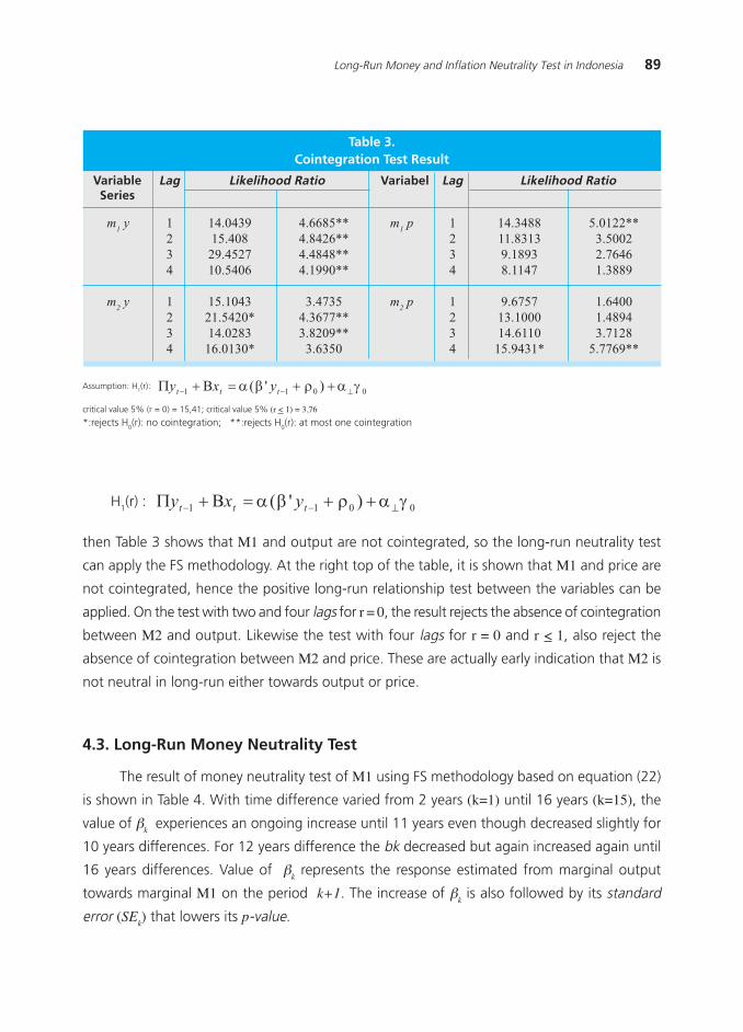
89Long-Run Money and Inflation Neutrality Test in Indonesia
then Table 3 shows that M1 and output are not cointegrated, so the long-run neutrality test
can apply the FS methodology. At the right top of the table, it is shown that M1 and price are
not cointegrated, hence the positive long-run relationship test between the variables can be
applied. On the test with two and four lags for r = 0, the result rejects the absence of cointegration
between M2 and output. Likewise the test with four lags for r = 0 and r < 1, also reject the
absence of cointegration between M2 and price. These are actually early indication that M2 is
not neutral in long-run either towards output or price.
4.3. Long-Run Money Neutrality Test
The result of money neutrality test of M1 using FS methodology based on equation (22)
is shown in Table 4. With time difference varied from 2 years (k=1) until 16 years (k=15), the
value of βk experiences an ongoing increase until 11 years even though decreased slightly for
10 years differences. For 12 years difference the bk decreased but again increased again until
16 years differences. Value of βk represents the response estimated from marginal output
towards marginal M1 on the period k+1. The increase of βk is also followed by its standard
error (SEk) that lowers its p-value.
Table 3.Cointegration Test Result
Lag Likelihood Ratio Variabel Lag Likelihood Ratio
Assumption: H1(r):
critical value 5% (r = 0) = 15,41; critical value 5% (r < 1) = 3,76
*:rejects H0(r): no cointegration; **:rejects H0(r): at most one cointegration
m1 y
m2 y
1
2
3
4
1
2
3
4
14.0439
15.408
29.4527
10.5406
15.1043
21.5420*
14.0283
16.0130*
4.6685**
4.8426**
4.4848**
4.1990**
3.4735
4.3677**
3.8209**
3.6350
m1 p
m2 p
14.3488
11.8313
9.1893
8.1147
9.6757
13.1000
14.6110
15.9431*
5.0122**
3.5002
2.7646
1.3889
1.6400
1.4894
3.7128
5.7769**
1
2
3
4
1
2
3
4
VariableSeries
H1(r) :
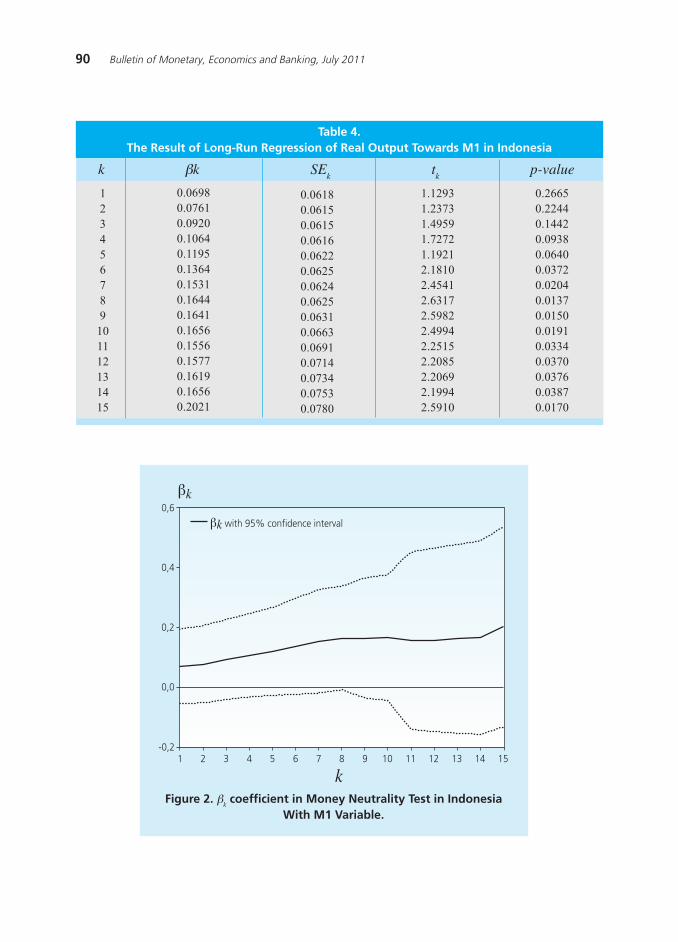
90 Bulletin of Monetary, Economics and Banking, July 2011
Table 4.The Result of Long-Run Regression of Real Output Towards M1 in Indonesia
k βk SEk
tk
p-value
1
2
3
4
5
6
7
8
9
10
11
12
13
14
15
0.0698
0.0761
0.0920
0.1064
0.1195
0.1364
0.1531
0.1644
0.1641
0.1656
0.1556
0.1577
0.1619
0.1656
0.2021
0.0618
0.0615
0.0615
0.0616
0.0622
0.0625
0.0624
0.0625
0.0631
0.0663
0.0691
0.0714
0.0734
0.0753
0.0780
1.1293
1.2373
1.4959
1.7272
1.1921
2.1810
2.4541
2.6317
2.5982
2.4994
2.2515
2.2085
2.2069
2.1994
2.5910
0.2665
0.2244
0.1442
0.0938
0.0640
0.0372
0.0204
0.0137
0.0150
0.0191
0.0334
0.0370
0.0376
0.0387
0.0170
Figure 2. βk coefficient in Money Neutrality Test in Indonesia
With M1 Variable.
-0,2
0,0
0,2
0,4
0,6
1 2 3 4 5 6 7 8 9 10 11 12 13 14 15
βk with 95% confidence interval
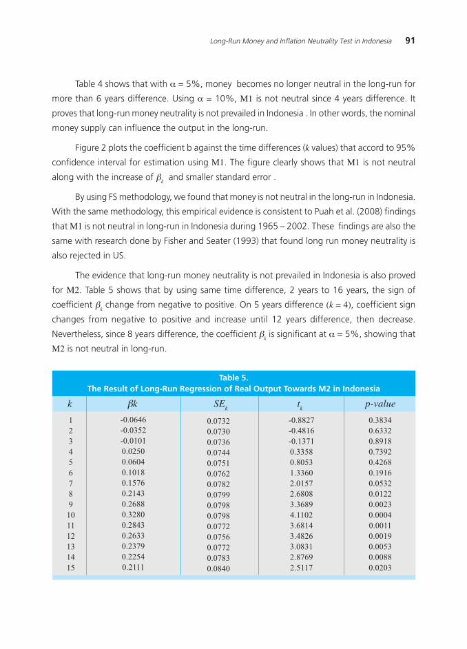
91Long-Run Money and Inflation Neutrality Test in Indonesia
Table 4 shows that with α = 5%, money becomes no longer neutral in the long-run for
more than 6 years difference. Using α = 10%, M1 is not neutral since 4 years difference. It
proves that long-run money neutrality is not prevailed in Indonesia . In other words, the nominal
money supply can influence the output in the long-run.
Figure 2 plots the coefficient b against the time differences (k values) that accord to 95%
confidence interval for estimation using M1. The figure clearly shows that M1 is not neutral
along with the increase of βk and smaller standard error .
By using FS methodology, we found that money is not neutral in the long-run in Indonesia.
With the same methodology, this empirical evidence is consistent to Puah et al. (2008) findings
that M1 is not neutral in long-run in Indonesia during 1965 √ 2002. These findings are also the
same with research done by Fisher and Seater (1993) that found long run money neutrality is
also rejected in US.
The evidence that long-run money neutrality is not prevailed in Indonesia is also proved
for M2. Table 5 shows that by using same time difference, 2 years to 16 years, the sign of
coefficient βk change from negative to positive. On 5 years difference (k = 4), coefficient sign
changes from negative to positive and increase until 12 years difference, then decrease.
Nevertheless, since 8 years difference, the coefficient βk is significant at α = 5%, showing that
M2 is not neutral in long-run.
Table 5.The Result of Long-Run Regression of Real Output Towards M2 in Indonesia
k βk SEk
tk
p-value
1
2
3
4
5
6
7
8
9
10
11
12
13
14
15
-0.0646
-0.0352
-0.0101
0.0250
0.0604
0.1018
0.1576
0.2143
0.2688
0.3280
0.2843
0.2633
0.2379
0.2254
0.2111
0.0732
0.0730
0.0736
0.0744
0.0751
0.0762
0.0782
0.0799
0.0798
0.0798
0.0772
0.0756
0.0772
0.0783
0.0840
-0.8827
-0.4816
-0.1371
0.3358
0.8053
1.3360
2.0157
2.6808
3.3689
4.1102
3.6814
3.4826
3.0831
2.8769
2.5117
0.3834
0.6332
0.8918
0.7392
0.4268
0.1916
0.0532
0.0122
0.0023
0.0004
0.0011
0.0019
0.0053
0.0088
0.0203
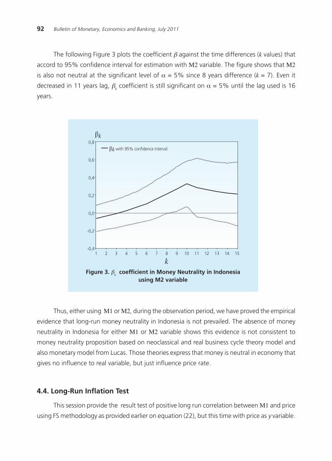
92 Bulletin of Monetary, Economics and Banking, July 2011
The following Figure 3 plots the coefficient β against the time differences (k values) that
accord to 95% confidence interval for estimation with M2 variable. The figure shows that M2
is also not neutral at the significant level of α = 5% since 8 years difference (k = 7). Even it
decreased in 11 years lag, βk coefficient is still significant on α = 5% until the lag used is 16
years.
Thus, either using M1 or M2, during the observation period, we have proved the empirical
evidence that long-run money neutrality in Indonesia is not prevailed. The absence of money
neutrality in Indonesia for either M1 or M2 variable shows this evidence is not consistent to
money neutrality proposition based on neoclassical and real business cycle theory model and
also monetary model from Lucas. Those theories express that money is neutral in economy that
gives no influence to real variable, but just influence price rate.
4.4. Long-Run Inflation Test
This session provide the result test of positive long run correlation between M1 and price
using FS methodology as provided earlier on equation (22), but this time with price as y variable.
Figure 3. βk coefficient in Money Neutrality in Indonesia
using M2 variable
1 2 3 4 5 6 7 8 9 10 11 12 13 14 15
βk with 95% confidence interval
-0,4
-0,2
0,0
0,2
0,4
0,6
0,8
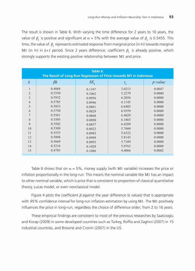
93Long-Run Money and Inflation Neutrality Test in Indonesia
The result is shown in Table 6. With varying the time difference for 2 years to 16 years, the
value of βk is positive and significant at α = 5% with the average value of β
k is 0.5455. This
time, the value of βk represents estimated response from marginal price (in ln) towards marginal
M1 (in ln) in k+1 period. Since 2 years difference, coefficient βk is already positive, which
strongly supports the existing positive relationship between M1 and price.
Table 6.The Result of Long-Run Regression of Price towards M1 in Indonesia
k βk SEk
tk
p-value
1
2
3
4
5
6
7
8
9
10
11
12
13
14
15
0.4068
0.5550
0.5932
0.5785
0.5853
0.5750
0.5561
0.5505
0.5502
0.5309
0.5535
0.5808
0.5669
0.5216
0.4785
0.1347
0.1062
0.0956
0.0946
0.0881
0.0829
0.0868
0.0890
0.0857
0.0922
0.0983
0.0999
0.0993
0.1028
0.1086
3.0213
5.2279
6.2056
6.1145
6.6403
6.9359
6.4029
6.1865
6.4209
5.7604
5.6322
5.8143
5.7109
5.0763
4.4066
0.0047
0.0000
0.0000
0.0000
0.0000
0.0000
0.0000
0.0000
0.0000
0.0000
0.0000
0.0000
0.0000
0.0000
0.0002
Table 6 shows that on α = 5%, money supply (with M1 variable) increases the price or
inflation proportionally in the long-run. This means the nominal variable like M1 has an impact
to other nominal variable, which is price that is consistent to proportion of classical quantitative
theory, Lucas model, or even neoclassical model.
Figure 4 plots the coefficient β against the year difference (k values) that is appropriate
with 95% confidence interval for long-run inflation estimation by using M1. The M1 positively
influences the price in long-run, regardless the choice of difference order; from 2 to 16 years.
These empirical findings are consistent to most of the previous researches by Saatcioglu
and Korap (2009) in some developed countries such as Turkey, Roffia and Zaghini (2007) in 15
industrial countries, and Browne and Cronin (2007) in the US.
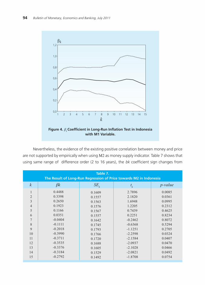
94 Bulletin of Monetary, Economics and Banking, July 2011
Nevertheless, the evidence of the existing positive correlation between money and price
are not supported by empirically when using M2 as money supply indicator. Table 7 shows that
using same range of difference order (2 to 16 years), the bk coefficient sign changes from
Figure 4. βk Coefficient in Long-Run Inflation Test in Indonesia
with M1 Variable.
1 2 3 4 5 6 7 8 9 10 11 12 13 14 150,0
0,2
0,4
0,6
0,8
1,0
1,2
k βk SEk
tk
p-value
1
2
3
4
5
6
7
8
9
10
11
12
13
14
15
0.4488
0.3398
0.2650
0.1923
0.1166
0.0351
-0.0404
-0.1111
-0.2018
-0.3990
-0.3711
-0.3535
-0.3376
-0.3184
-0.2792
0.1609
0.1557
0.1563
0.1576
0.1567
0.1557
0.1642
0.1745
0.1793
0.1766
0.1720
0.1688
0.1605
0.1529
0.1492
2.7896
2.1820
1.6948
1.2205
0.7439
0.2251
-0.2462
-0.6368
-1.1251
-2.2598
-2.1584
-2.0937
-2.1028
-2.0821
-1.8708
0.0085
0.0361
0.0995
0.2312
0.4625
0.8234
0.8072
0.5294
0.2705
0.0324
0.0407
0.0470
0.0466
0.0492
0.0754
Table 7.The Result of Long-Run Regression of Price towards M2 in Indonesia
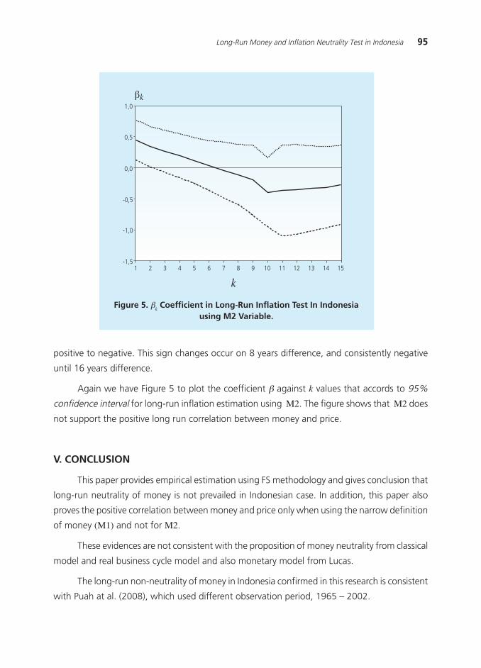
95Long-Run Money and Inflation Neutrality Test in Indonesia
positive to negative. This sign changes occur on 8 years difference, and consistently negative
until 16 years difference.
Again we have Figure 5 to plot the coefficient β against k values that accords to 95%
confidence interval for long-run inflation estimation using M2. The figure shows that M2 does
not support the positive long run correlation between money and price.
V. CONCLUSION
This paper provides empirical estimation using FS methodology and gives conclusion that
long-run neutrality of money is not prevailed in Indonesian case. In addition, this paper also
proves the positive correlation between money and price only when using the narrow definition
of money (M1) and not for M2.
These evidences are not consistent with the proposition of money neutrality from classical
model and real business cycle model and also monetary model from Lucas.
The long-run non-neutrality of money in Indonesia confirmed in this research is consistent
with Puah at al. (2008), which used different observation period, 1965 √ 2002.
Figure 5. βk Coefficient in Long-Run Inflation Test In Indonesia
using M2 Variable.
1 2 3 4 5 6 7 8 9 10 11 12 13 14 15-1,5
-1,0
-0,5
0,0
0,5
1,0

96 Bulletin of Monetary, Economics and Banking, July 2011
The implication is straightforward that monetary policy to stabilize fluctuation in
macroeconomic does really matter, Monetary expansion in long-run, can stimulate the output,
although it can also stimulate inflation. So, in Inflation Targeting Framework, the monetary
authority can keep focusing on inflation without ignoring the importance of the role of money
supply towards the long-run increase of output .
97Long-Run Money and Inflation Neutrality Test in Indonesia
Bae, S. and R. Ratti (2000), ≈Long-Run Neutrality, High Inflation, and Bank Insolvencies in
Argentina and Brazil,∆ Journal of Monetary Economics, 46: 581-604.
Barro, R (1997), Macroeconomics, 5th edition, Canbridge, MA: MIT Press.
Boschen, J.F. and C.M. Otrok (1994), ≈Long-Run Neutrality and Superneutrality in an ARIMA
Framework: Comment,∆ American Economic Review, 84: 1470-1473.
Browne, F. and D. Cronin (2007), ≈Commodity Prices, Money and Inflation,∆ ECB Working
Paper Series, 738 (March): 1-33.
Chen, S.W. (2007), ≈Evidence of the Long-Run Neutrality of Money: the Case of South Korea
and Taiwan,∆ Economics Bulletin, 64(3): 1-18.
Coe, P.J. and J.M. Nason (2004), ≈Long-Run Monetary Neutrality and Long-Horizon
Regressions,∆ Journal of Applied Econometrics, 19 (3): 355-373
Dickey, D. and W.A. Fuller (1979), ≈Distribution of the Estimates for Autoregressive Time Series
with a Unit Root,∆ Journal of the American Statistical Society, 74: 427-431.
Dewald, W.G. (1998), ≈Historical U.S. Money Growth, Inflation, and Inflation Credibility,∆ Federal
Reserve Bank of St. Louis Review, 80:13√24.
Dwyer, G.P. and R. W. Hafer (1999), ≈Are Money Growth and Inflation Still Related?,∆ Federal
Reserve Bank of Atlanta Economic Review, Second Quarter: 32-43.
Engle, R.F. and C.W.J. Granger (1987), ≈Cointegration and Error Correction: Representation,
Estimation and Testing,∆ In Engle R.F. and C.W.J. Granger (1991), Long-Run Economic
Relationships: Readings in Cointegration, 81-111. New York: Oxford University Press.
Fisher, M.E and J.J. Seater (1993), ≈Long-Run Neutrality and Superneutrality in an ARIMA
Framework,∆ American Economic Review, 83(3): 402-415.
Gujarati, D.N. and D.C. Porter (2009), Basic Econometrics, 5th Edition, New York: McGraw-Hill.
Hume, D. (1752), ≈Of Money, Of Interest, and Of the Balance of Trade,∆ In Essays, Moral,
Political, and Literary, Reprinted in Hume, 1955, Writings on Economics, Eugene
Rotwein ed.
Diakses dari http://www.econlib.org/library/LFBooks/Hume/hmMPL.html
Johansen, S. (1995), Likelihood-based Inference in Cointegrated Vector Autoregressive Models,
New York: Oxford University Press.
REFERENCES
98 Bulletin of Monetary, Economics and Banking, July 2011
King, R.G. and M.W. Watson (1997), ≈Testing Long-Run Neutrality,∆ Federal Reserve Bank of
Richmond Economic Quarterly, 83(3): 69-101.
Lucas, R.E. (1972), ≈Expectations and the Neutrality of Money,∆ Journal of Economic Theory,
4(2): 103√124.
__________ (1980), ≈Two Illustrations of the Quantity Theory of Money,∆ American Economic
Review, 70: 1005√1014.
___________(1995), ≈Monetary Neutrality. Prize Lecture,∆ December 7, 1995. Diakses dari http:/
/nobelprize.org/economics/laureates/1995/lucas-lecture.pdf.
McCandless, G.T., Jr. and W.E. Weber (1995), ≈Some Monetary Facts,∆ Federal Reserve Bank of
Minneapolis Quarterly Review, 19(3): 1-11.
Noriega, A.E (2004), ≈Long-Run Monetary Neutrality and the Unit-Root Hypothesis: Further
International Evidence,∆ North American Journal of Economics and Finance, 15(2): 179-
197.
Noriega, A.E., L.M. Soria and R. Velazquez (2005), ≈International Evidence on Monetary Neutrality
under Broken Trend Stationary Models,∆ Mimeo. Diakses dari http://repec.org/esLATM04/
up.7482.1080751251.pdf
Oi, H., S. Shiratsuka, and T. Shirota (2004), ≈On Long-Run Monetary Neutrality in Japan,∆
Monetary and Economic Studies, 22(3): 79 √ 113
Olekalns, N. (1996), ≈Some Further Evidence on the Long-Run Neutrality of Money,∆ Economics
Letters, 50(3): 393-98.
Phillips, P.C.B., and P. Perron (1988), ≈Testing for a Unit Root in Time Series Regression,∆
Biometrika, 75(2): 335-346.
Puah, C.H., M.S. Habibullah and S.A. Mansor (2008), ≈On the Long-Run Monetary Neutrality:
Evidence from the SEACEN Countries,∆ Journal of Money, Investment and Banking, Issue 2:
50-62.
Ran, J. (2005), ≈Is There Long-Run Money Neutrality under Different Exchange Rate Regimes?,∆
Pacific Economic Review, 10(3): 361-370.
Roffia, B. and A. Zaghini (2007), ≈ Excess Money Growth and Inflation Dynamics,∆ ECB Working
Paper Series, 749: 1-40.
Romer, D. (2001), Advanced Macroeconomics, Second Edition, New York: McGraw-Hill.
Rolnick, A.J. and W.E. Weber (1997), ≈Inflation, Money, and Output under Alternative Monetary
Standards,∆ Federal Reserve Bank of Minneapolis Research Department, Staff Report 175.
Saatcioglu, C. and L. Korap (2009), ≈The Search for Co-Integration Between Money, Prices and
Income: Low Frequency Evidence from the Turkish Economy,∆ Panoeconomicus, 1: 55-72.
Serletis, A. and Z. Koustas (1998), ≈International Evidence on the Neutrality of Money,∆ Journal
of Money, Credit and Banking, 30 (1): 1√25.

99Long-Run Money and Inflation Neutrality Test in Indonesia
ƒƒƒ, and ƒƒƒ (2001), ≈Monetary Aggregation and the Neutrality of Money,∆ Economic
Inquiry, 39 (1): 124√138. Diakses dari http://econpapers.repec.org/article/oupecinqu/
Shelley, G.L. and F.H. Wallace (2003), ≈Testing for Long Run Neutrality of Money in Mexico,∆
Diakses dari http://129.3.20.41/eps/mac/papers/0402/0402003.pdf
Wallace, F.H. and L.F. Cabrera-Castellanos (2006), ≈Long Run Money Neutrality in Guatemala,∆
MPRA Paper 4025, University Library of Munich, Germany, revised 2006. Diakses dari http:/
/129.3.20.41/eps/mac/papers/

100 Bulletin of Monetary, Economics and Banking, July 2011
This page is intentionally left blank
101
WRITING GUIDANCE
1. The paper should be original and should not violate any copyrights. The submitted paper
should have never been published or not being submitted to other publisher. The copyright
of the published paper is retained to the author.
2. The Bulletin of Monetary Economics and Banking provide a financial incentive between IDR
1,000,000 to IDR 3,000,000.
3. The paper should be sent in 2 formats (1) Microsoft Word (*.doc) and (b) portable digital file
(*.PDF). The 2 files should be sent to the following mail address:
[email protected] and Cc to: [email protected]
You may save your files in CD and send it to the following Editorial Address:
BULLETIN OF MONETARY ECONOMICS AND BANKING
Directorate of Economic Research and Monetary Policy-Bank Indonesia
Building Syafruddin Prawiranegara, 20th Floor
JI. M. H. Thamrin No.2 Central Jakarta, Indonesia
Ph. +62-21-3818202, Fax. +62-21- 3800394
4.4.4.4.4. To avoid missing fonts or other compatibility issue, any special characters or mathematicalTo avoid missing fonts or other compatibility issue, any special characters or mathematicalTo avoid missing fonts or other compatibility issue, any special characters or mathematicalTo avoid missing fonts or other compatibility issue, any special characters or mathematicalTo avoid missing fonts or other compatibility issue, any special characters or mathematical
expression (equations, symbol, matrix, etc.) must be written using Microsoft Equation.expression (equations, symbol, matrix, etc.) must be written using Microsoft Equation.expression (equations, symbol, matrix, etc.) must be written using Microsoft Equation.expression (equations, symbol, matrix, etc.) must be written using Microsoft Equation.expression (equations, symbol, matrix, etc.) must be written using Microsoft Equation.
5. The submitted paper should contain (i) an abstract of maximum one page A4, (ii) keywords
and (iii) JEL classification code. See the JEL code at http://www.aeaweb.org/journal/
jel_class_system.html.
6. The paper must contain the followings:
The background, the aim of the paper and its distinction to previous study
Theory and review of literatures
Methodology (quantitative methodology is preferred)
Result and analysis
Policy and further study implication
7. The citation should be in footnote and not in endnote.
8. The reference must obey the following rule:
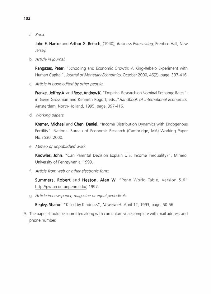
102 Bulletin of Monetary Economics and Banking, October 2010
a. Book:
John E. HankeJohn E. HankeJohn E. HankeJohn E. HankeJohn E. Hanke and Arthur G. ReitschArthur G. ReitschArthur G. ReitschArthur G. ReitschArthur G. Reitsch, (1940), Business Forecasting, Prentice-Hall, New
Jersey.
b. Article in journal:
Rangazas, PeterRangazas, PeterRangazas, PeterRangazas, PeterRangazas, Peter. ≈Schooling and Economic Growth: A King-Rebelo Experiment with
Human Capital∆, Journal of Monetary Economics, October 2000, 46(2), page. 397-416.
c. Article in book edited by other people:
Frankel, Jeffrey AFrankel, Jeffrey AFrankel, Jeffrey AFrankel, Jeffrey AFrankel, Jeffrey A. and Rose, Andrew KRose, Andrew KRose, Andrew KRose, Andrew KRose, Andrew K. ≈Empirical Research on Nominal Exchange Rates∆,
in Gene Grossman and Kenneth Rogoff, eds.,∆Handbook of International Economics.
Amsterdam: North-Holland, 1995, page. 397-416.
d. Working papers:
Kremer, MichaelKremer, MichaelKremer, MichaelKremer, MichaelKremer, Michael and Chen, DanielChen, DanielChen, DanielChen, DanielChen, Daniel. ≈Income Distribution Dynamics with Endogenous
Fertility∆. National Bureau of Economic Research (Cambridge, MA) Working Paper
No.7530, 2000.
e. Mimeo or unpublished work:
Knowles, JohnKnowles, JohnKnowles, JohnKnowles, JohnKnowles, John. ≈Can Parental Decision Explain U.S. Income Inequality?∆, Mimeo,
University of Pennsylvania, 1999.
f. Article from web or other electronic form:
Summers, RobertSummers, RobertSummers, RobertSummers, RobertSummers, Robert and Heston, Alan WHeston, Alan WHeston, Alan WHeston, Alan WHeston, Alan W. ≈Penn World Table, Version 5.6∆
http://pwt.econ.unpenn.edu/, 1997.
g. Article in newspaper, magazine or equal periodicals:
Begley, SharonBegley, SharonBegley, SharonBegley, SharonBegley, Sharon. ≈Killed by Kindness∆, Newsweek, April 12, 1993, page. 50-56.
9. The paper should be submitted along with curriculum vitae complete with mail address and
phone number.