Embed Size (px)
Citation preview

Technical Appendices
Business Climate Rankings and the California Economy
Jed Kolko, David Neumark, and Marisol Cuellar Mejia
Contents
Appendix A. Business Climate Indexes
Appendix B. Related Academic Research
Appendix C. Data and Methods
Appendix D. Detailed Findings
References
Supported with funding from the David A. Coulter Family Foundation and the Donald Bren Foundation

http://www.ppic.org/main/home.asp Technical Appendices Business Climate Rankings and the California Economy 2
Appendix A: The Business Climate Indexes
State Business Climate Indexes
Assessments of the business climate typically rank states or localities using a combination of measures, and the sets of measures vary widely. For example, the Tax Foundation, the Cato Institute, the American Legislative Exchange Council, the Pacific Research Institute, and the Small Business and Entrepreneurship Council all publish state rankings that focus strictly on taxes, regulations, and fiscal policy measures.1 The Beacon Hill Institute’s index includes factors that could affect economic growth even if they are not policy-determined, like crime rates, academic research and development spending, and air quality, along with tax indicators.2 Some indexes focus more narrowly on technology and the new economy, such as the SNEI.3 And yet others emphasize equity and quality of life measures, such as those of the Corporation for Enterprise Development.
In addition to these differences in the broad emphasis of different business climate indexes, the indexes also vary widely in terms of the specific variables and years covered, the weighting of the variables, the extent to which they have been validated, etc. In this section, we provide a brief overview of the indexes we study—enough, we hope, to provide some idea about the types of factors emphasized by each index. The first column of Table A1 lists the indexes included in our study and the institution that creates the index (as well as the years covered).4 The next two columns describe the focus of each index, and list the 14 categories of variables (which we have created) covered by each index; a full list of these categories is discussed below.5
Two significant features of these indexes are apparent. First, the indexes aim to capture different facets of the policy and economic environment, as captured (in some cases, at least) by the name of the index. Compare, for example, the Small Business Survival Index (SBSI) with the Fiscal Policy Report Card on the Nation’s Governors (FPRCNG). Thus, it would not be at all surprising if states are ranked differently depending on the index, and if the indexes varied in the extent to which they predict economic outcomes.
Second, the institutions that create these indexes in some cases may construct indexes according to a particular agenda or mission. For example, the Economic Freedom Index (EFI) is put out by the Pacific Research Institute, whose mission is to “champion freedom, opportunity, and personal responsibility for all individuals by advancing free-market policy solutions.”6 In contrast, the DRCS-P focuses on quality of life, equity, and employment, earnings, and job quality; this index is created by the Corporation for Enterprise Development, which describes itself as “[d]riven to create a more robust, fair and sustainable economy for all of us, … fueled by the belief that there is a tremendous amount of untapped potential in low-income people
1 See Dubay and Atkins (2006), Slivinski (2006), Laffer and Moore (2007), and Fisher (2005). 2 See Beacon Hill Institute (2008). 3 See Atkinson and Andes (2008). 4 We also examined the ALEC-Laffer State Economic Competitiveness Index, created by the American Legislative Exchange Council/ALEC, the California Economic Performance Card, created by the California Foundation for Commerce and Education, and Best States for Business created by Forbes Magazine. However, the first is available only for 2008 and 2009, the second only for 2008, and the third from 2006 through 2009, years that are beyond our sample period or hardly overlap. In addition, there is not sufficient detail available for Forbes’ Best States for Business, making it impossible to evaluate how the index was generated in terms of variables, sources, weights, and aggregation methods. 5 The second column lists the focus of the index as stated by the creating institution. The third column gives a more objective summary of the types of factors included. The notes to the table provide references for the source documents, which provide more detail. 6 See http://liberty.pacificresearch.org/about/default.asp (viewed November 4, 2009).

http://www.ppic.org/main/home.asp Technical Appendices Business Climate Rankings and the California Economy 3
and distressed communities.”7 Business climate indexes created by an institution with a point of view are not categorically dubious—it is an empirical question how well such indexes predict economic performance. But this does highlight that indexes vary widely, and the fact that the factors emphasized by a particular index sometimes have a relationship with the institution’s point of view might suggest that the index does not necessarily emphasize the factors most predictive of economic performance.
Although the third column of Table A1 lists our categories of variables covered by the different indexes, the table does not provide detail on the specific variables that go into these categories, nor the share of the weight that each index puts on the different categories. We provide more information on the composition of the indexes in two steps. First, in Table 2 (main text) we group the 14 categories we have created into three broad classes: taxes and costs; productivity (and quality of life); and other. We then show the weights (relative to a total of 100) that each index puts on these 14 categories as well as the broad class.8 This table clearly highlights differences between indexes that emphasize very different components of the economic and policy environment. For example, the table shows that the SBTC, and some other indexes (SBSI, CDBI, EFI, EFINA, and FPRCNG) focus heavily on taxes, costs, and regulation and litigation, the DRCS-P index emphasizes quality of life measures, and the SNEI emphasizes human capital, new businesses, and technology. In addition, though, the table reveals differences within these groups—such as the sole emphasis of the SBTC index on taxes, and the considerably heavier emphasis of the EFI index on regulation and litigation.
Second, in Table A2 we provide a much more detailed list of the variables within each of our 14 categories that go into each index. This, too, is informative for interpreting the indexes. For example, we see that the SBTC index weighs a broad range of tax rates, while others (the SCI and CDBI indexes) try to summarize all of this information in a single tax burden, and yet others (such as the FPRCNG) emphasize a small set of taxes. Similarly, the table reveals the kinds of variables used to capture quality of life (such as crime rates and infant mortality) and equity (such as the poverty rate, and inequality in the income distribution).
To show yet another way how the indexes are related, Table A3 shows the correlations across states of the different indexes (in each case, averaged across years). The order in which the indexes are displayed in this table is not random, as explained below. Note, though, that among the first five indexes (SNEI, DRCS-P, DRCS-DC, DRCS-BV, and SCI) the correlations are positive, and in almost every case quite high. On the other hand, the correlations of these five indexes with the next five (SBTC, SBSI, CDBI, EFI, and EFINA) are mostly negative, and in many cases (especially when they are not negative) quite small. Conversely, the correlations among these latter fives indexes are uniformly positive, and again quite large. Finally, the correlations of the FPRCNG index with the other ten indexes, shown in the last row of Table A3, are generally small and vary in sign.
To more systematically assess the impressions given by these correlations, we performed a variety of cluster analyses on the average index values, generally finding that there were two distinct clusters, one that generally included the first five indexes listed above, and one that generally included the second set of five indexes. The last index (FPRCNG) was more or less randomly assigned to one cluster or the other. For this reason—coupled with the information on what factors and policies the indexes weight—we refer to the first set of indexes, including SNEI, DRCS-P, DRCS-DC, DRCS-BV, and SCI, as belonging to the “productivity
7 See http://development.cfed.org/focus.m (viewed November 4, 2009). 8 The main text explains how these weights are constructed.

http://www.ppic.org/main/home.asp Technical Appendices Business Climate Rankings and the California Economy 4
cluster,” and the second set, including SBTC, SBSI, CDBI, EFI, and EFINA, as belonging to the “taxes-and-costs cluster.” We did not assign FPRCNG to either cluster.
Table A4 shows how the 50 states rank on the business climate indexes, averaged across the years for which the index is available.9 In the three right-hand columns we report the mean, minimum, and maximum for the state across the index averages. The table reveals that states’ positions in the rankings can vary wildly from one index to another. Indeed, the last column of the table shows that the smallest difference between the minimum and maximum average ranking for states is 21, and for 16 states the range is 40 or higher. Thus, essentially all states are ranked quite differently across the business climate indexes. This, of course, is the primary motivation for our efforts to determine the empirical content of these indexes. Many states rank consistently within a cluster, such as Massachusetts performing well across the productivity indexes and California and New York both performing poorly across the taxes-and-costs indexes. But even among indexes in the same “cluster” a state’s rankings can sometimes vary considerably: Texas, for instance, ranges from 5th (EFINA) to 26th (CDBI) in the taxes-and-costs cluster and from 6th (DRCS-BV) to 47th (DRCS-P) in the productivity cluster.
As Table A1 showed, each index is available for at least some years—sometimes many and sometimes few. For most of the indexes, the inter-temporal correlations (available upon request) are very high, exceeding 0.7 or 0.8 even for observations eight or nine years apart. One mild exception is for the DRCS-BV index, for which these correlations dip to near 0.5. More notable is the FPRCNG index, for which the correlations are frequently near zero or negative, and the implied autocorrelation function does not indicate a positive (but lower) correlation between nearby observations that tails off, but is rather quite erratic. This difference in patterns for the FPRCNG index likely stems from the inclusion of and relatively heavy weight placed on policy variables that fluctuate more (see Table A2), in particular the changes in per capita proposed and actual general fund spending.
The information presented thus far has a few implications for our empirical strategy. First, the high inter-temporal correlations imply that there is little variation in an index within states over time. This implies that there is little to be learned from regression models with fixed state effects. Consequently, our regression models primarily identify the effects of variation in business climate indexes and sub-indexes from cross-state variation, incorporating an extensive set of controls for state characteristics.10
Second, given that the indexes are typically available only for a subset of years (see Table A1), and that there is often not much overlap between the years available for different indexes, for the most part we study one index at a time for the years for which that index is available. The fact that the inter-temporal correlations of the indexes are high is reassuring on this issue, as it implies that we are relatively unlikely to get answers that would vary in other years—at least because of changes in the index.
Third, even within each cluster, indexes have different emphases. Those that report sub-indexes will allow for deeper analysis of the policies contributing to the relationships we will observe between these indexes
9 Because we average across years, in any one column all 50 values of the rank do not necessarily appear. This averaging implies that the variation across states discussed below is not simply driven by single-year outliers, but rather by more systematic differences in how the different business climate indexes rank states. 10 Moreover, the within-state variation over time that does exist may reflect measurement error, given the numerous subjective and somewhat ad hoc decisions that go into constructing the indexes, as well as actual errors in measurement. It is well known that in such a case controlling for fixed state effects can bias the estimated effects of the indexes toward zero, and can easily result in more biased estimates than cross-sectional regressions without fixed effects, especially when the regression model includes a comprehensive list of relevant control variables, which increases the noise-to-signal ratio in the mismeasured variables.

http://www.ppic.org/main/home.asp Technical Appendices Business Climate Rankings and the California Economy 5
and economic growth. In fact, because a sub-index reflects a narrower, more tightly-defined set of policy variables than an index made up of multiple sub-indexes, the relationship with economic growth may be stronger for some individual sub-indexes than for the indexes they belong to.
State Business Climate Sub-Indexes
Several of the business climate indexes also define and report scores for sub-indexes that are combined to produce the final index score and ranking. We analyze the composition of the three taxes-and-costs indexes (SBTC, EFINA, EFI) and four productivity indexes (SNEI and the three DRCS indexes) that present information about sub-indexes. Each of these indexes has between two and five sub-indexes, which are listed and described in Table A5. Table A5 also shows the weight each sub-index gets in calculating the index. For the productivity indexes, the table also shows the weight of variables in each sub-index that we consider to be outcomes: the DRCS-P “employment” sub-index, for instance, consists entirely of variables that we consider to be economic outcomes, like employment growth, rather than policy-related factors potentially affecting economic outcomes. In analyzing the relationship between these sub-indexes and economic growth, we construct alternative versions of sub-indexes that strip out components that we consider to be economic outcomes (see Appendix D).
These sub-index labels require some deciphering. EFINA’s “labor market freedom” sub-index includes components for minimum wage legislation, government share of total employment, and unionization, for instance. To compare sub-indexes better, we apply our own 14 categories in Table 2 to the sub-indexes and present the results in Tables A6a and A6b of the main text. Both EFINA’s “takings and discriminatory taxation” sub-index (EFINA-TDT) and EFI’s “fiscal” index (EFI-F) are measures of what we call “tax rates and tax burden,” and no other sub-index in EFINA or EFI includes similar tax measures. Particularly confusing is that only one of the three variables in EFINA’s “size of government” sub-index (EFINA-SG) — “general consumption expenditures by government as percentage of GDP”—falls under what we classify as size of government. The other two variables in EFINA-SG—transfers and subsidies as a percent of GDP and social security payments as a percent of GDP—fall into our “welfare and transfer payments” category. In contrast, EFI’s “government size” (EFI-GS) sub-index falls entirely into our “size of government” category (see Table A6a), since it includes state and local total expenditures as a percent of GSP, the size of the government workforce, and citizen representation.11 We consider “size of government” to be independent of the composition of government expenditure, preferring to include compositional measures of welfare, transfers, and subsidies under our “welfare and transfer payments” category. Our categorization in Tables A6a and A6b should make clear that the sub-indexes with similar names as given by the organizations that create the indexes—like EFINA-SG and EFI-GS—might actually measure quite different policies, whereas sub-indexes given different names—like EFINA-SG and EFI-WS, or EFINA-TDT and EFI-F—might actually measure quite similar policies.
11 This latter is measured as a combination of the average of total number of government units, and legislators per million people.

http://www.ppic.org/main/home.asp Technical Appendices Business Climate Rankings and the California Economy 6
Table A1. Business climate indexes
Index/ranking, institution, and years
Stated focus of index Categories1 Comparability across
years Validity checks as reported by institution
State New Economy Index (SNEI), Progressive Policy Institute (1999, 2002) Information, Technology and Innovation Foundation and Kauffman Foundation (2007, 2008)2
Compatibility of state’s economy with “New Economy”
Business incubation; human capital; technology, knowledge jobs, and digital economy
Indicators and methods of constructing index not identical across years
States that score higher appear to create jobs at a slightly faster rate than lower-ranking states. Between 2002 and 2006, there was virtually no correlation (0.02) between employment growth and SNEI. Claim that job creation is not necessarily the best measure of long-term economic wellbeing, especially if growth comes in the form of low-paying jobs. Reports that growth in per capita income is more important, and that SNEI was positively correlated with growth in per capita incomes between 2002 and 2006 (0.34).
Development Report Card for the States─Performance (DRCS-P), Corporation for Enterprise Development (2001–2007)3
Opportunities for employment, income, and improving quality of life
Quality of life; equity; employment, earnings, and job quality
Measures included in sub-index in each year can change, which can also lead to changes in weights if number of variables in a sub-index (which are equally-weighted) changes
Does not empirically test the effectiveness of their indexes in predicting economic outcomes. However, their framework and measures were reviewed by technical advisors and representatives from the business community, labor, government and community development organizations.
Development Report Card for the States─ Development Capacity (DRCS-DC), Corporation for Enterprise Development (2001–2007) 3
Capacity for future development
Cost of doing business (excl. taxes); quality of life; business incubation; human capital; infrastructure; technology, knowledge jobs, and digital economy
Measures included in sub-index in each year can change, which can also lead to changes in weights if number of variables in a sub-index (which are equally-weighted) changes
Does not empirically test the effectiveness of their indexes in predicting economic outcomes. However, their framework and measures were reviewed by technical advisors and representatives from the business community, labor, government and community development organizations.
Development Report Card for the States─Business Vitality (DRCS-BV), Corporation for Enterprise Development (2001–2007) 3
Dynamism of the state's large and small businesses
Business incubation; technology, knowledge jobs, and digital economy
Measures included in sub-index in each year can change, which can also lead to changes in weights if number of variables in a sub-index (which are equally-weighted) changes
Does not empirically test the effectiveness of their indexes in predicting economic outcomes. However, their framework and measures were reviewed by technical advisors and representatives from the business community, labor, government and community development organizations.
State Competitiveness Index (SCI), Beacon Hill Institute (2001–2008)
Long-term competitiveness for attracting and incubating new businesses and growth of existing firms
Cost of doing business (excl. taxes); size of government; tax rates and tax burden; quality of life; welfare and transfer payments; employment, earnings, and job quality; business incubation; human capital; infrastructure; technology, knowledge jobs, and digital economy
Consistent across years The Beacon Hill Institute tries to answer the question: Do the indexes of state competitiveness explain affluence and growth? To answer that, they use a regression analysis that attempts to predict differences in real per capita income across states at a point in time on the basis of the SCI and real per-capita income in the previous year.
State Business Tax Climate Index (SBTC), Tax Foundation (2003–2009)
Tax rates Tax rates and tax burden Methods change each year, but old index values reconstructed based on new methods, so index consistent across years
The Tax Foundation does not verify empirically the validity of the SBTC. Instead, they rely on the existing economic literature that has found a strong relationship between taxes and economic growth.

http://www.ppic.org/main/home.asp Technical Appendices Business Climate Rankings and the California Economy 7
Index/ranking, institution, and years
Stated focus of index Categories1 Comparability across
years Validity checks as reported by institution
Small Business Survival Index (SBSI), Small Business and Entrepreneurship Council (1996–2008)
Government-imposed or government-related costs affecting investment, entrepreneurship, and business
Cost of doing business (excl. taxes); size of government; tax rates and tax burden; regulation and litigation; quality of life; infrastructure
No discussion in documents, but number of variables included has increased from 9 in 1996 to 34 in the 2008 edition
The Small Business and Entrepreneurship Council does not verify empirically the validity of the SBSI. They argue that its SBSI is “supported by sound economic reasoning and fundamentals. That is, the inclusion of each measure meets a basic economic common sense test. For good measure, a wide body of economic analysis further backs up this economic common sense.”
Cost of Doing Business Index (CDBI), Milken Institute (2002–2007)
Fundamental business costs, including labor, taxes, real estate and electricity
Cost of doing business (excl. taxes); tax rates and tax burden
Methods change over time No empirical testing of effectiveness of index in predicting economic outcomes.
Economic Freedom Index (EFI), Pacific Research Institute (1999, 2004, 2008)
Government is toward free enterprise and consumer choice; rights of individuals to pursue their interests through voluntary exchange of private property under rule of law
Cost of doing business (excl. taxes); size of government; tax rates and tax burden; regulation and litigation; welfare and transfer payments
Different indicators and weights used in 1999 and 2004
From constructed list of indicators, explored different subsets of variables and weighting techniques, choosing the index with the strongest predictive power to explain human migration across the 50 U.S. states. Afterwards, they test empirically the relationship between their final Economic Freedom Index and two outcome variables (total personal income growth and change in total employment growth) finding a positive and significant relationship between economic freedom and growth.
Economic Freedom Index of North America (EFINA), The Fraser Institute / National Center for Policy Analysis (1981–2005)
Restrictions on economic freedom imposed by governments: takings and discriminatory taxation; size of government; and labor market freedom
Cost of doing business (excl. taxes); size of government; tax rates and tax burden; welfare and transfer payments
Consistent across years To test whether or not there is a positive relationship between economic growth and economic freedom, they use annual observations on each of the components from 1981 to 2005 and run state fixed-effects models. They report that GDP per-capita is positively associated with the degree of economic freedom as measured by their index.
Fiscal Policy Report Card on the Nation's Governors (FPRCNG), Cato Institute (1992–2008, biennial)
Fiscal performance of governors in terms of restraining the growth of taxes and spending
Cost of doing business (excl. taxes); size of government; tax rates and tax burden
2008 report card uses a somewhat different methodology than prior Cato report cards
No direct test of index, but claims that selected research reports argument that fiscal stringency produces economic growth.
NOTES: See Table A2 for a detailed list of variables used in the indexes. 1 These are category labels that we have assigned. They are often, although not always, the same as those used by the institutions that create the indexes. See Table 2 in the main text for the weights the indexes place on each of these categories. 2Although the SNEI has been produced by two different institutions, the author of all four reports computing the SNEI is the same (Robert Atkinson). 3The DRCS indexes go back to 1987, but only the information beginning in 2001 was available on-line.
SOURCES (for latest version of each index):
SNEI: http://www.kauffman.org/uploadedfiles/2008_state_new_economy_index_120908.pdf (viewed November, 2008); DRCS_P, DRCS_DC, DRCS_BV: http://cfed.org/knowledge_center/research/DRC/ (viewed March, 2011); SCI: http://www.beaconhill.org/Compete08/BHIState08-FINAL.pdf (viewed November, 2008); SBTC: http://www.taxfoundation.org/files/bp58.pdf (viewed November, 2008); SBSI: http://www.sbecouncil.org/uploads/sbsi%202008%5B1%5D1.pdf (viewed December, 2008); CDBI: http://www.milkeninstitute.org/pdf/2007CostofDoingBusiness.pdf (viewed November, 2008); EFI: http://special.pacificresearch.org/pub/sab/entrep/2008/Economic_Freedom/map.html (viewed November, 2008); EFINA: http://www.freetheworld.com/efna2008/EFNA_Complete_Publication.pdf (viewed November, 2008); FPRCNG: http://www.cato.org/pubs/pas/pa-624.pdf (viewed November, 2008).
Table A1 (continued)

http://www.ppic.org/main/hom Technical Appendices Business Climate Rankings and the California Economy 8
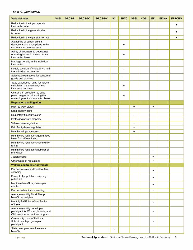
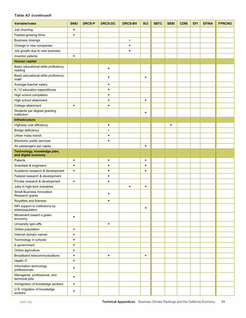
Table A2. Variables in business climate indexes
Variable/index SNEI DRCS-P DRCS-DC DRCS-BV SCI SBTC SBSI CDBI EFI EFINA FPRCNG
Cost of doing business (excluding taxes)
Workers compensation costs − − − Minimum wage − − − − Union membership rate − − Electricity cost − − − − − Rent costs − Size of government Full-time equivalent government employees per 100 residents − − − −
Trend in government spending − State expenditures per capita − − State debt per capita − General consumption expenditures by government as % of GDP −
Average annual percentage change in per capita general fund spending proposed by the governor
−
Average annual percentage change in actual per capita general fund spending
−
Average dollar value of proposed and enacted tax and fee changes −
Bond rating: S&P's/Moody's composite + +
Budget surplus as % of GSP + Tax rates and tax burden Top personal income tax rate − − − − Income threshold for top marginal income tax rate +
Top corporate income tax rate − − − Top capital gains tax rate − − − Unemployment insurance tax rate − − − Sales tax rate − − Property tax rate − Gas tax rate − − − Diesel tax rate − − − Cigarettes tax rate − − Distilled spirits tax rate − − Sales, gross receipts, and excise tax burden − − −
Property tax burden − − − Estate, inheritance, and/or gift taxes − − −
Measure of tax burden − − − − Tax limitation status + Internet access tax − Additional income tax on S-corporations − −
Indexed personal income tax rates + + Corporate alternative minimum tax − − Individual alternative minimum tax − − Reduction in the top personal income tax rate +
http://www.ppic.org/main/hom Technical Appendices Business Climate Rankings and the California Economy 9
Variable/index SNEI DRCS-P DRCS-DC DRCS-BV SCI SBTC SBSI CDBI EFI EFINA FPRCNG
Reduction in the top corporate income tax rate +
Reduction in the general sales tax rate +
Reduction in the cigarette tax rate + Availability of certain credits, deductions and exemptions in the corporate income tax base −
Ability of taxpayers to deduct net operating losses in the corporate income tax base +
Marriage penalty in the individual income tax − Double taxation of capital income in the individual income tax − Sales tax exemptions for consumer goods and services − State experience rating formulas in calculating the unemployment insurance tax base +
Charging in proportion to base period wages in calculating the unemployment insurance tax base +
Regulation and litigation Right-to work status + + Legal liability costs - Regulatory flexibility status + Protecting private property + Video choice regulation + Paid family leave regulation − Health savings accounts + Health care regulation: guaranteed issue for self-employed −
Health care regulation: community rating −
Health care regulation: number of mandates − −
Judicial sector − Other types of regulations − Welfare and transfer payments Per capita state and local welfare spending −
Percent of population receiving public aid −
Medicare benefit payments per enrollee −
Per capita Medicaid spending − Average monthly Food Stamp benefit per recipient −
Monthly TANF benefit for family of three −
Average monthly benefit per participant for Women, Infants, and Children special nutrition program
−
Commodity costs of National School Lunch program per participant
−
State unemployment insurance benefits −
Table A2 (continued)

http://www.ppic.org/main/hom Technical Appendices Business Climate Rankings and the California Economy 10
Variable/index SNEI DRCS-P DRCS-DC DRCS-BV SCI SBTC SBSI CDBI EFI EFINA FPRCNG
Social security payment − Transfers and subsidies − Quality of life Crime rate − − − Better Government Association integrity index +
Travel time to work − Homeownership rate + Population without health insurance − − Net migration + Infant mortality − − Children at or below 200% of the poverty line without health insurance
−
Teen pregnancy − Heart disease − Charitable giving + Voting rate + Cost of urban housing − − Households with installed phones + Rate of nonfederal physicians per 100,000 inhabitants +
Conversion of cropland to other uses +
Equity Poverty rate − Income inequality − Income inequality increase − Disparity between rural and urban areas −
Employment, earnings and job quality
Employment growth: long term + Employment growth: short term + Unemployment rate − − Private sector layoffs − Average annual pay + Average annual pay growth + Employer health coverage + Working poor − Involuntary part-time employment − % of adults in labor force + Business incubation Initial public offerings + + + New companies + + + Venture capital + + + Income from dividends, interest and rent +
Small Business Investment Company financing +
Loans to small businesses + Deposits in commercial banks and savings institutions +
Gazelle jobs +
Table A2 (continued)
http://www.ppic.org/main/hom Technical Appendices Business Climate Rankings and the California Economy 11
Variable/index SNEI DRCS-P DRCS-DC DRCS-BV SCI SBTC SBSI CDBI EFI EFINA FPRCNG
Job churning + Fastest-growing firms + Business closings − Change in new companies + Job growth due to new business + Inventor patents + Human capital Basic educational skills proficiency: reading +
Basic educational skills proficiency: math + +
Average teacher salary + K–12 education expenditures + High school completion + High school attainment + + College attainment + + Students per degree granting institution +
Infrastructure Highway cost efficiency + + Bridge deficiency − Urban mass transit + Electronic public services + Air passengers per capita + Technology, knowledge jobs, and digital economy
Patents + + + Scientists & engineers + + + Academic research & development + + + Federal research & development + Private research & development + + Jobs in high-tech industries + + Small Business Innovation Research grants +
Royalties and licenses + NIH support to institutions by state/population +
Movement toward a green economy +
University spin-offs + Online population + Internet domain names + Technology in schools + E-government + Online agriculture + Broadband telecommunications + + + Health IT + Information technology professionals +
Managerial, professional, and technical jobs +
Immigration of knowledge workers + U.S. migration of knowledge workers +
Table A2 (continued)
http://www.ppic.org/main/hom Technical Appendices Business Climate Rankings and the California Economy 12
Variable/index SNEI DRCS-P DRCS-DC DRCS-BV SCI SBTC SBSI CDBI EFI EFINA FPRCNG
High-tech jobs + Manufacturing value-added + + High-wage traded services + Resource efficiency/environment Per capita energy consumption − Use of alternative energy + Toxic release inventory − − Vehicle miles traveled − Rate of recycled waste + Greenhouse gas emissions − − Air quality + + External sector Exports + Incoming FDI per capita, dollars + + Export focus of manufacturing and services +
Strength of traded sector + Industrial diversity + Percent of population born abroad +
NOTES: Table shows the variables included as of the last year for which the index was available at the time of writing. See Table A1. The list of variables can vary year-to-year. We do not list every single variable when there is more than one variable that would fit under the same label in this table (e.g., multiple crime rates). Variables are not always measured in exactly the same fashion in each index in which they are included. For example, academic research and development is included in three indexes. In DRCS-DC it corresponds to expenditures per capita, while in SCI it corresponds to expenditures per $1,000 of GSP. Another example is initial public offerings, which appears as well in three indexes. In SNEI it is measured as a share of total worker earnings; in SCI as a share of GSP; and in DRCS-BV as proceeds of initial public offerings per 1,000 firms. The positive signs mean that the variable enters positively into the index, and vice versa. For example, referring to the first row of the table, a state with higher workers compensation costs, everything else equal, would have a lower score in the SCI.
Table A2 (continued)

http://www.ppic.org/main/home.asp Technical Appendices Business Climate Rankings and the California Economy 13
Table A3. Correlations of average indexes across states, 1992–2009
SNEI DRCS-P DRCS-DC DRCS-BV SCI SBTC SBSI CDBI EFI EFINA FPRCNG
SNEI 1
DRCS-P 0.55* 1
DRCS-DC 0.75* 0.70* 1
DRCS-BV 0.72* 0.29* 0.59* 1
SCI 0.53* 0.74* 0.72* 0.23 1
SBTC -0.05 -0.12 -0.08 -0.13 0.14 1
SBSI -0.14 -0.17 -0.13 -0.02 0.02 0.76* 1
CDBI -0.72* -0.37* -0.40* -0.45* -0.12 0.18 0.25 1
EFI -0.26 -0.010 -0.12 -0.16 0.22 0.57* 0.53* 0.61* 1
EFINA 0.03 -0.03 -0.01 0.23 0.06 0.48* 0.64* 0.26 0.62* 1
FPRCNG 0.09 0.07 -0.03 0.09 0.10 0.18 0.33* -0.07 0.07 0.14 1
NOTES: The table reports correlations of the average rank across years for each index. * indicates statistically significantly different from zero at the 5% level. All 50 states are included.

http://www.ppic.org/main/home.asp Technical Appendices Business Climate Rankings and the California Economy 14
Table A4. Average state ranks by index, 1992–2009
State SNEI DRCS-P DRCS-DC DRCS-BV SCI SBTC SBSI CDBI EFI EFINA FPRCNG Mean Min Max Alabama 45 40 45 16 45 18 9 14 17 12 32 27 9 45 Alaska 27 40 42 42 21 3 15 41 39 46 N/A 32 3 46 Arizona 17 33 37 33 30 27 23 27 19 7 27 25 7 37 Arkansas 48 43 45 28 46 36 27 11 17 25 27 32 11 48 California 4 31 17 4 20 45 46 47 47 43 31 31 4 47 Colorado 6 14 6 1 5 12 12 26 6 12 14 10 1 26 Connecticut 6 5 8 10 16 38 35 47 44 28 21 23 5 47 Delaware 7 9 7 15 14 9 26 42 12 2 35 16 2 42 Florida 21 31 33 28 32 5 8 28 27 6 16 21 5 33 Georgia 20 30 25 20 32 24 21 25 14 11 17 22 11 32 Hawaii 35 27 45 45 44 23 48 49 33 43 25 38 23 49 Idaho 23 21 32 26 10 30 30 7 2 34 26 22 2 34 Illinois 18 35 17 10 36 23 19 37 37 22 30 26 10 37 Indiana 34 33 27 30 36 11 14 18 20 12 17 23 11 36 Iowa 41 13 23 39 15 44 40 5 21 27 30 27 5 44 Kansas 31 27 18 26 16 31 35 15 7 23 27 23 7 35 Kentucky 43 43 40 24 38 34 26 15 36 28 19 31 15 43 Louisiana 44 50 48 37 48 35 27 21 34 14 34 36 14 50 Maine 29 14 37 30 30 39 46 28 36 47 25 33 14 47 Maryland 5 8 9 21 20 29 25 38 32 21 30 22 5 38 Massachusetts 1 9 7 4 2 32 33 48 40 23 11 19 1 48 Michigan 23 26 23 25 30 26 12 40 35 35 16 26 12 40 Minnesota 13 2 1 10 7 42 46 41 38 37 19 23 1 46 Mississippi 50 49 49 41 50 19 10 11 19 24 17 31 10 50 Missouri 34 26 30 32 24 17 18 16 13 16 27 23 13 34 Montana 42 33 28 40 25 9 38 4 20 43 29 28 4 43 Nebraska 32 14 24 36 12 44 32 10 23 18 20 24 10 44 Nevada 26 27 42 32 35 4 2 32 13 16 20 23 2 42 New Hampshire 11 1 18 22 8 8 11 33 7 7 18 13 1 33 New Jersey 5 17 12 8 36 48 43 45 46 34 28 29 5 48 New Mexico 27 46 37 37 37 27 39 32 35 39 13 34 13 46 New York 12 23 18 21 35 49 45 49 50 48 12 33 12 50 North Carolina 26 40 29 24 29 42 38 24 26 13 31 29 13 42 North Dakota 42 32 19 44 12 34 24 2 17 32 25 26 2 44 Ohio 30 32 18 25 41 47 38 25 40 41 33 33 18 47 Oklahoma 39 41 42 26 40 19 28 8 10 30 20 28 8 42 Oregon 15 23 10 28 14 9 40 20 33 37 39 24 9 40 Pennsylvania 22 22 10 10 33 26 18 33 45 30 23 25 10 45 Rhode Island 20 13 31 29 27 49 48 35 48 48 26 34 13 49 South Carolina 36 34 40 23 39 26 14 8 15 13 13 24 8 40 South Dakota 45 13 32 46 14 2 1 1 7 7 11 16 1 46 Tennessee 35 39 35 21 36 17 10 12 25 1 23 23 1 39 Texas 15 47 32 6 25 7 7 26 19 5 13 18 5 47 Utah 12 16 6 18 5 14 26 14 4 19 21 14 4 26 Vermont 21 3 27 30 10 43 41 38 37 39 22 28 3 43 Virginia 9 9 9 9 13 15 14 30 5 6 26 13 5 30 Washington 4 20 3 26 6 12 5 37 36 40 21 19 3 40 West Virginia 49 48 46 49 48 36 35 14 34 49 29 40 14 49 Wisconsin 33 8 17 24 19 38 27 30 31 37 21 26 8 38 Wyoming 43 18 24 46 9 1 3 22 6 24 26 20 1 46

http://www.ppic.org/main/home.asp Technical Appendices Business Climate Rankings and the California Economy 15
Table A5. Description of business climate sub-indexes
Sub-index name Description / variables included Sub-index weight
Outcomes weight
Knowledge jobs (SNEI-KJ)
Employment in IT occupations in non-IT industries as a share of total jobs; managers, professionals, and technicians as a share of the total workforce; educational attainment of the workforce; educational attainment of recent migrants from abroad; educational attainment of recent migrants within the U.S.; manufacturing value-added per production hour worked as a percentage of the national average, adjusted by industrial sector; share of employment in traded-service sectors in which the average wage is above the national median for traded services
24.1 0.0
Globalization (SNEI-G)
Value of exports per manufacturing and service worker; percentage state workforce employed by foreign companies 9.6 0.0
Economic dynamism (SNEI-ED)
Jobs in gazelle companies (firms with annual sales revenue that has grown 20% or more for four straight years) as a share of total employment; number of new startups and business failures, combined, as share of the total firms in state; number of Deloitte Technology Fast 500 and Inc. 500 firms as share of total firms; number and value of initial public stock offerings of companies as a share of total worker earnings; number of entrepreneurs starting new businesses; number of independent inventor patents per capita
21.7 33.3
Digital economy (SNEI-DE)
Internet users as share of the population; number of Internet domain names per firm; computer and Internet use in schools; utilization of digital technologies in state government; percentage of farmers with Internet access and using computers for business; adoption of residential broadband services and median download speed; number of prescriptions routed electronically as a percentage of total number of prescriptions eligible for electronic routing
20.5 0.0
Innovation capacity (SNEI-IC)
Jobs in electronics manufacturing, software and computer-related services, telecommunications, and biomedical industries as a share of total employment; scientists and engineers as percentage of workforce; number of patents issued to companies or individuals per worker; industry R&D as percentage of total worker earnings; non-industrial R&D as percentage of GSP; change in energy consumption per capita and change in renewable energy consumed as percentage of total energy; venture capital invested as share of worker earnings
24.1 0.0
Variable weighting
SNEI assigns different weights to each sub-index, and different weights to each variable in each sub-index.
Employment (DRCS-P-EMP)
10-year and annual percent change in employment; unemployment rate; extended mass layoff events (private, non-farm), per establishment 20.0 100.0
Earnings and job quality (DRCS-P-EJQ)
Annual pay for workers covered by unemployment insurance; percent change in annual pay for all workers covered by unemployment insurance; percent of non-elderly population covered by employer-based health plans; percent of households with at least one worker whose combined income is no more than 150% of the poverty line; percent of employees who work part-time for economic reasons
20.0 80.0
Equity (DRCS-P-E)
Percent of population in households with incomes below the poverty level; ratio of mean income of families in the top quintile to mean income of families in the bottom quintile; percent change in the ratio of mean income of families (family income) in the top quintile to mean income of families in the bottom quintile; composite index score of six economic performance measures that compare absolute value differences between non-metropolitan and metropolitan counties within a state
20.0 25.0

http://www.ppic.org/main/home.asp Technical Appendices Business Climate Rankings and the California Economy 16
Sub-index name Description / variables included Sub-index weight
Outcomes weight
Quality of life (DRCS-P-QL)
Net domestic migration rate; rate of infant (under one year) deaths per live birth; percent of children under 19 years of age at or below 200% of the poverty line without health insurance; birth rate for females aged 15–19; death rate from coronary heart disease; homeownership rate; average charitable contribution as percentage of adjusted gross income; percent of people (18 and over) voting in the November 2004 elections; rate of serious (violent and property) crimes per capita
20.0 0.0
Resource efficiency (DRCS-P-RE)
Per capita energy consumption; percent of energy consumed from renewable resources; total toxic release per capita; annual vehicle miles traveled, per capita; percent of solid waste recycled; and metric tons of carbon dioxide equivalent per capita
20.0 0.0
Competitiveness of existing business (DRCS-BV-CEB)
Traded sector earnings per worker; rate of firm terminations; machinery and equipment expenditures as a percent of manufacturing value added; Herfindahl index of diversity among industries within the state's traded sector
50.0 25.0
Entrepreneurial energy (DRCS-BV-EE)
Number of companies applying for new employment identification numbers per worker; percent change in companies applying for new employment identification numbers; number of jobs created by new establishments for firms with fewer than 500 employees per new establishment; percent of total wage and salary jobs in high technology industries; proceeds of initial public offerings per firm
50.0 80.0
Human resources (DRCS-DC-HR)
Percent of 4th grade students at or above proficient in reading; percent of 4th grade students at or above proficient in math; average teacher salary relative to comparable wages; per pupil expenditures adjusted for wages, for pre-K–12 students; high school completion rate of 18–24 year-olds; percent heads of household with at least 12 years of education; percent heads of households with at least four years of college
20.0 0.0
Innovation assets (DRCS-DC-IA)
Number of employed doctoral scientists and engineers per worker; number of science and engineering graduate students in doctorate-granting institutions per capita; number of High-Speed Lines per capita; R&D expenditures at universities and colleges per capita; federal obligations for R&D per capita; amount of private research and development per worker; SBIR grants awarded per worker; gross license income per worker; number of patents issued per capita; number of university spin-outs per $1 billion university R&D spending
20.0 0.0
Financial resources (DRCS-DC-FR)
Annual state personal income per capita from dividends, interest, and rent; venture capital investments per worker; total SBIC financing per worker; cumulative amount of loans under $1 million per worker 20.0 25.0
Amenities resources & natural capital (DRCS-DC-AR)
Average cost of electricity per kilowatt hour; average of fair market rent schedules for a standard two-bedroom unit of housing, metropolitan areas, as percent of median metropolitan family income; state population without primary care within ready economic and geographic reach per capita; percent change of land in farms; proportion of persons living in counties designated by the EPA as "non-attainment," where air pollution levels persistently exceed the national ambient air quality standards for one or more of seven air pollutants
20.0 0.0
Infrastructure resources (DRCS-DC-IR)
Ratio of cost effectiveness of state-owned road system to national average; percent of bridges on and off federal aid system rated as deficient; all urban public mass transit systems' carrying capacity, in annual vehicle revenue miles per capita; and E-government index score based on availability of contact information, publications, databases, portals, and number of online services by state government
20.0 0.0
Variable weighting
In DRCSs, sub-index variables are weighted equally in each sub-index, and then the sub-indexes are weighted equally in the final index; each variable’s weight in the final index depends on the number of variables in its sub-index.
Table A5 (continued)

http://www.ppic.org/main/home.asp Technical Appendices Business Climate Rankings and the California Economy 17
Sub-index name Description / variables included Sub-index weight
Outcomes weight
Corporate tax (SBTC-CTI)
Tax rate sub-index: corporate income tax top rate; bracket structure; gross receipts rate Tax base sub-index: availability of certain credits, deductions and exemptions; ability of taxpayers to deduct net operating losses; smaller tax base issues (under gross receipts tax, the three tax base criteria replaced by availability of deductions from gross receipts for employee compensation costs and cost of goods sold)
19.4 0.0
Individual income tax (SBTC-IITI)
Tax rate sub-index: top marginal tax rate and graduated rate structure (takes into account starting points of top brackets, number of brackets, and average width of brackets) Tax base sub-index: marriage penalty; capital gains taxation; double taxation of capital income; minor base issues
29.2 0.0
Sales tax (SBTC-STI)
Tax rate sub-index: state-level rate and combined state-local rate Tax base sub-index: whether base includes variety of business-to-business transactions such as agricultural products, services, machinery, computer software, and leased or rented items; whether base includes goods and services typically purchased by consumers; excise tax rate on products such as gasoline, diesel fuel, tobacco, spirits, and beer
21.5 0.0
Property tax (SBTC-PTI)
Tax rate sub-index: property tax collection, measured both per capita and as percentage of personal income; capital stock tax rates and maximum payments Tax base sub-index: whether levies wealth taxes such as inheritance, estate, gift, inventory, and intangible property
15.7 0.0
Unemployment insurance tax (SBTC-UITI)
Tax rate sub-index: rates levied in the most recent year; statutory rate schedules that could be implemented depending on the state of the economy and the UI fund Tax base sub-index: experience rating formulas; charging methods; and smaller factors
14.2 0.0
Variable weighting
Each sub-index includes a tax rate and tax base component, equally weighted. Scalar variables are on scale of zero (worst) to 10 (best), and are weighted equally. If component includes scalar and dummy variables then weights are 80 percent for scalar variables and 20 percent for dummy variables.
Size of government (EFINA-SG)
General consumption expenditures by government as a percent of GDP; transfers and subsidies as percent of GDP; social security payments (includes unemployment insurance, disability, public pensions) as percent of GDP
33.3 0.0
Labor market freedom (EFINA-LMF)
Minimum wage legislation; government employment as a percent of total state employment; union density 33.3 0.0
Takings and discriminatory taxation (EFINA-TDT)
Total tax revenue as percent of GDP; top marginal income tax rate and income threshold at which applies; indirect tax revenue as a percent of GDP; sales taxes collected as percent of GDP 33.3 0.0
Variable weighting Each variable is weighted equally in the sub-index.
Fiscal (EFI-F)
Average days required for work to cover taxes; per capita state tax revenue; per capita state and local property tax revenue; tax burden on high-income family; per capita state government death and gift tax revenue; per capita state government severance tax revenue; personal income taxes; sales taxes; excise taxes; license taxes; corporate taxes; state debt; tax exemptions
34.9 0.0
Table A5 (continued)

http://www.ppic.org/main/home.asp Technical Appendices Business Climate Rankings and the California Economy 18
Sub-index name Description / variables included Sub-index weight
Outcomes weight
Regulatory (EFI-R)
Licensing requirements for non-health professions; licensing requirements for health professions; continuing education requirements for selected professions; percent land owned by federal government; purchasing regulations; public school regulation; labor legislation; full-time-equivalent employees of state public utilities commissions; corporate constituency statutes; property rights legislation; strictness of state gun laws; state seat belt laws; state provisions for minimum age for driver's licenses; full-time-equivalent employees of insurance regulation organization; state legislation regarding environmental health
34.2 0.0
Welfare spending (EFI-WS)
Per capita state and local welfare spending; percent of population receiving public aid; Medicare benefit payments per enrollee; per capita Medicaid spending; average monthly Food Stamp benefit per recipient; monthly TANF benefit for family of three; average monthly benefit per participant for Women, Infants, and Children Special Nutrition Program; commodity costs of National School Lunch Program per participant
37.3 0.0
Government size (EFI-GS)
State and local total expenditures as a percent of GSP; size of government workforce; citizen representation (avg. of total number of government units, and legislators per million people) 6.3 0.0
Judicial (EFI-J)
Number of resident active attorneys; Attorney General salary; judges' compensation; judges' terms; judges' selection method; state has Illinois Brick Repealer statutes (which restrict anti-trust suits); tort reform; medical-liability reform
-12.6 0.0
Variable weighting Sub-indexes are averages of state ranks on each variable.
NOTES: SNEI weights correspond to the values in the 2008 edition; DRCS weights correspond to the values in the 2007 edition; and SCI weights correspond to the values in the 2008 edition. SBTC sub-index weights described are for 2006 and 2007; sub-index weighting was different for 2003 and 2004. EFI sub-index weights described are for 2004; sub-index weighting was different in 1999. Note that variables in some sub-indexes are described relative to state GSP, and others relative to GDP; these are interchangeable terms. Underlined are the variables that we consider are outcomes. The EFI sub-indexes are weighted according to a principal components analysis, and the negative weight on the judicial sub-index presumably reflects a weak or negative correlation with other EFI sub-indexes.
Table A5 (continued)

http://www.ppic.org/main/home.asp Technical Appendices Business Climate Rankings and the California Economy 19
Table A6a. Distribution of weights of components of business climate sub-indexes by categories (%), taxes-and-costs cluster
SBTC-CTI
SBTC-IITI
SBTC-STI
SBTC-PTI
SBTC-UITI
EFINA-SG
EFINA-LMF
EFINA-TDT
EFI- F
EFI- R
EFI- WS
EFI- GS
EFI- J
Taxes and costs category percentage
Cost of doing business (excluding taxes) 66.67 1.33
Size of government 33.33 33.33 7.69 100.00
Tax rates and tax burden 100.00 100.00 100.00 100.00 100.00 100.00 92.31
Regulation and litigation 98.67 100.00
Welfare and transfer payments 66.67 100.00
Productivity category percentage
Quality of life
Equity
Employment, earnings and job quality
Business incubation
Human capital
Infrastructure
Technology, knowledge jobs, and digital economy
“Other” category percentage
Resource efficiency / environment
External sector
Sub-index weight 19.43 29.15 21.5 15.72 14.2 33.33 33.33 33.33 34.86 34.22 37.3 6.27 -12.6
NOTES: EFI weights correspond to the values in the 2004 edition (http://special.pacificresearch.org/pub/sab/entrep/2004/econ_freedom/00_summary.html, viewed July 2010); SBTC weights correspond to the values in the 2007 edition (http://www.hopewelltwp.org/bp52.pdf, page 9, viewed July 2010); and EFINA weights to the values in the 2008 edition (http://www.freetheworld.com/efna2008/EFNA_Complete_Publication.pdf, page 95, viewed July 2010).

http://www.ppic.org/main/home.asp Technical Appendices Business Climate Rankings and the California Economy 20
Table A6b. Distribution of weights of components of business climate sub-indexes by categories (%), productivity cluster
SNEI-KJ
SNEI- G
SNEI-ED
SNEI-DE
SNEI-DC
DRCS-P-
EMP
DRCS-P-
EJQ
DRCS-P- E
DRCS-P- QL
DRCS -P- RE
DRCS -BV- CEB
DRCS -BV- EE
DRCS-DC-HR
DRCS-DC- IA
DRCS-DC-FR
DRCS-DC-AR
DRCS-DC- IR
Taxes and costs category percentage
Cost of doing business (excluding taxes) 20.0
Size of government
Tax rates and tax burden
Regulation and litigation
Welfare and transfer payments
Productivity category percentage
Quality of life 100.0 60.0
Equity 100.0
Employment, earnings and job quality 100.0 100.0
Business incubation 100.0 15.0 25.0 80.0 100.0
Human capital 20.0 100.0
Infrastructure 100.0
Technology, knowledge jobs, and digital economy
80.0 100.0 85.0 25.0 20.0 100.0
"Other" category percentage
Resource efficiency / environment 100.0 20.0
External sector
100.0 50.0
Sub-index weight 24.1 9.6 21.7 20.5 24.1 20.0 20.0 20.0 20.0 20.0 50.0 50.0 20.0 20.0 20.0 20.0 20.0
NOTES: SNEI weights correspond to the values in the 2008 edition (http://www.itif.org/files/2008_State_New_Economy_Index.pdf, page 70, viewed July 2010); and DRCS weights correspond to the values in the 2007 edition (http://cfed.org/knowledge_center/research/DRC/, viewed July 2010).

http://www.ppic.org/main/home.asp Technical Appendices Business Climate Rankings and the California Economy 21
Appendix B: Related Academic Research
Assessment of Business Climate Indexes
Erickson (1987) reviews the development of business climate indexes in the United States. Concerns about state and regional business climates go back to the period just after World War II, when the U.S. South and West were competing more directly with the North for manufacturing industry at the same time that manufacturing was declining. Taxes have always been at the center of discussions about the “business climate,” with other issues rising or falling in importance with the times, such as workforce education during the growth of high-technology industries in the 1960’s and energy costs after the oil crisis in the 1970’s. Modern business climate indexes began with the 1975 Fantus Company index, prepared for the Illinois Manufacturers’ Association; the Alexander Grant & Company (later, Grant Thornton) index, prepared for the Conference of State Manufacturers’ Associations, first in 1979; and the Inc. magazine Report Card on the States, first published in 1981. Numerous indexes followed later. Erickson (1987) criticizes this first wave of business climate indexes for their simplicity, while acknowledging the considerable media attention they get and crediting business climate indexes for encouraging local and state governments to examine their tax, regulatory, infrastructure, and education policies more closely.
Three academic studies assess the relationship between these early indexes and economic outcomes. Plaut and Pluta (1983) use a business climate measure based on the Fantus and Alexander Grant & Company indexes. These two indexes covered a range of taxes, business costs, and other measures. For each of these indexes, a more favorable ranking is positively correlated with higher production, employment, and capital stock; all of these outcomes are measured for the manufacturing sector.1 Plaut and Pluta regress each manufacturing outcome on the composite business climate measure and other explanatory variables, including several, like union activity and tax rates, which are already included in one or both of the business climate indexes. The business climate measure has a positive and statistically significant relationship with the changes in employment and capital stock, though not with changes in output. A concern is that their output measures cover the periods 1967–1972 and 1972–1977, and the business climate indexes were published in 1975 and 1979 and therefore may be based on data measured after the outcomes are measured, although if the indexes change slowly over time this may not matter much.
Skoro (1988) assesses the relationship between economic growth and two business climate indexes: the Grant Thornton index and Inc. magazine’s index. Whereas the Grant Thornton index was weighted toward taxation, Inc. focused on capital availability, state aid to business, labor costs and quality, and recent business activity. Skoro argues that although the Grant Thornton index claims to measure the business climate only for manufacturers and the Inc. index claims to measure the business climate only for small businesses, they should be evaluated, at least in part, on their ability to predict overall economic growth. Based on bivariate correlations, Skoro finds that both indexes have a positive relationship with measures of employment growth, though only some correlations are statistically significant; the relationship with the change in per capita income is not statistically significant. Skoro compares these correlations with the correlations between 1 Note that, in the study, a higher value of the index means a worse ranking, so the signs reported by Plaut and Pluta are the opposite of how we describe the results here. In the ensuing discussion, we make a similar change when needed to be consistent with how we describe results for business climate indexes in this report. A reader comparing our discussion to what is reported in these studies should keep this in mind.

http://www.ppic.org/main/home.asp Technical Appendices Business Climate Rankings and the California Economy 22
employment growth and growth measures (population, employment, and income) from the previous decade and finds that, in many cases, the lagged growth measures show a stronger correlation with the growth outcomes than the business climate indexes do. Because both business climate indexes include components measuring lagged economic growth, Skoro concludes that the indexes may be “useless” because lagged economic growth by itself is often more highly correlated with later growth than the indexes are. This case would have been more convincing had he included both the business climate indexes and lagged growth measures together in a regression.
Holmes (1998) found a positive effect of right-to-work laws on manufacturing employment in counties that border a state with the opposite right-to-work status. As a specification check on his finding that manufacturing grows faster in right-to-work states, he includes the Fantus business climate index as a control, to see whether right-to-work status matters per se or as a proxy for general business climate. Once the Fantus index is included, the right-to-work variable ceases to have a statistically significant effect on manufacturing employment.
In recent years, another set of studies has assessed the usefulness of a second wave of business climate indexes, including many of the same indexes we consider in this report. In a wide-ranging critique of business climate indexes, Fisher (2005) assesses how well five indexes predict economic performance. He is particularly critical of the “arbitrary” weighting of components in the construction of most indexes, contrasting the indexes to regression models that assign weights empirically based on predictions of economic performance. He finds that the 2001 SBSI index is positively correlated with some measures of “small business vitality and entrepreneurship,” like the share of new firms among all firms and the share of employment in rapidly growing firms, but not other measures like patents issued; many of his outcome measures, though, are from earlier than 2001, the year of the SBSI index he assesses, and he looks only at bivariate correlations.2 In assessing the SBTC index, Fisher finds no correlation or a negative correlation with measures of state average and marginal tax rates, and on these grounds argues that any predictive power of the SBTC for economic performance—which he does not test—would be spurious.
As also discussed in Fisher (2005), the creators of the SCI do their own assessment, finding that the index is positively correlated with the one-year change in per capita real income. Fisher finds this relationship is very sensitive to the state-level deflator used to calculate real income; he also finds that the only sub-index within the SCI that predicts income growth is one he dubs “income correlates,” suggesting the positive relationship is tautological. In assessing his fourth index, the Cato Institute’s FPRCNG, Fisher points out that Cato’s self-assessment of the index may suffer from reverse causality: several of the well-ranked tax-cutting states that grew faster during the 1990’s cut taxes later in that decade after increasing taxes earlier in the decade. Fisher’s own analysis regresses per-capita income growth in 2000–2003 on 2000 per capita income and a modified version of the index (restricting the measure to actual tax changes up to 2000, not those proposed by governors but not enacted); this modified index had no statistically significant relationship with per-capita income growth.
In discussing the EFI, Fisher reviews the creators’ own assessment rather than conducting his own. In constructing the EFI, more than two hundred rankings were averaged into several sub-indexes. The weights assigned to these sub-indexes in the final index were chosen to maximize the predictive power of the index
2 The outcome measures he correlates with the SBSI index themselves are components of the State New Economy Index (SNEI), which is one of the indexes we assess.

http://www.ppic.org/main/home.asp Technical Appendices Business Climate Rankings and the California Economy 23
for state differences in net domestic migration flows. Fisher criticizes EFI’s self-assessment for using their 2004 index to help predict differences in 2000 per-capita income; as with the Cato self-assessment, this, too, begs the question of reverse causality.3
Fisher’s review of these business climate indexes is the most thorough description of multiple indexes we have found. He raises the important points that often business climate indexes use proxies that fail to measure accurately what they claim to; that including economic outcome measures in indexes that purport to predict economic outcomes is circular; and that index construction often involves weighting components arbitrarily rather than based on their actual predictive power. His evaluation of these indexes is a useful starting point, but can be criticized on several grounds. First, he restricts his tests of predictive power to simple correlations or regressions in which the only control other than the index is a lagged level of the dependent variable. This approach will only detect very short-term effects of policy, due to the inclusion of the lagged dependent variable. Second, by assessing indexes on their own terms—such as comparing the tax-focused SBTC with other tax measures—Fisher is sensitive to the creators’ intentions but makes it difficult to compare the predictive power of multiple indexes. Even when an index is intended to reflect only the tax burden or only the climate for entrepreneurship, these outcomes are assumed to contribute to broader performance measures—like output, employment, or income—and are of only marginal policy interest if they do not. Furthermore, by tailoring tests to fit each index, Fisher is open to criticism that the tests are selectively or arbitrarily chosen.
In contrast, Bittlingmayer et al. (2005) use a uniform framework that facilitates comparison across indexes, making their study the most similar in the literature to ours. They consider the effects of numerous business climate indexes on growth in aggregate wages, population, employment, and the number of non-farm proprietorships. However, in lieu of controls for other state-level variables that could be correlated with both the business climate index and outcome measures, they include only counties on state borders: the unit of observation is a pair of counties straddling a state border, and all variables (the business climate indexes and the outcome growth rates) are ratios of the two counties’ values. Results are mixed: roughly half of the twelve indexes have a positive, statistically significant relationship with most or all economic outcomes in most years, and the other half have no relationship or a negative relationship with these outcomes. Indexes tend to have a consistent effect across the four outcome measures. The authors point out that even the indexes showing a positive relationship explain little of the variation in economic outcomes. Also, indexes more narrowly focused on tax policies were more likely to have positive relationships with growth than were broader measures.
Two concerns arise with Bittlingmayer et al. (2005). First, their study looks at economic outcomes for four time periods: 1970–1980, 1980–1990, 1990–2000, and 1992–2002, but they use only a single year of each business climate index; for seven of the twelve indexes they use values from 1999 or later. Though they demonstrate that the correlation across years (up to nine years apart) for a given index ranges from 0.58 to near 1 (usually in the 0.7–0.8 range), the relationship between many indexes and outcomes is sensitive to the time period of the outcome, and in some cases the positive relationship is stronger for early years than for later years. As with many of the self-assessments described above in the review of Fisher (2005),
3 Documents about other indexes also demonstrate how well they predict past economic outcomes. The American Legislative Exchange Council “Rich States, Poor States” report shows (their Table 9) that the top 10 states in the 2009 index exhibited faster growth in GDP, per-capita income, aggregate income, and population in 1997-2007 than the bottom 10 states. See http://www.alec.org/am/pdf/tax/09RSPS/26969_REPORT_full.pdf (viewed 11/12/09). We do not include this index in our assessment because we look at indexes up to 2007, which we test against subsequent economic performance, and this index is first available in 2008.

http://www.ppic.org/main/home.asp Technical Appendices Business Climate Rankings and the California Economy 24
Bittlingmayer et al. (2005) could be picking up the effect of growth on state policies (for example, fast-growing states could have expanding tax bases and therefore can lower tax rates while maintaining constant revenue) rather than an effect of policies on growth.
A second concern is that border areas may not be representative of entire states. In particular, coastal states—where a disproportionate share of U.S. economic activity is located—tend to have their economic and population centers right on the coast since oceans facilitate trade and transportation. In states with smaller coastlines, like New York or Pennsylvania, economic centers might be both on the coast and near state borders; in states with larger coastlines, like California and Florida, the vast majority of economic activity is far from state borders, and border areas of those states are economically distinct from the rest of the state. Furthermore, economic activity in border areas is probably more sensitive to differences in state tax and regulatory policies since both sides of the border share similar economic conditions and may be in the same labor market. A business in a border area could move over the border to take advantage of a more favorable tax or regulatory climate while retaining much of its workforce, while a business far from a state border would face much higher costs of replacing workers in order to move to a different state.
As part of a report measuring Michigan’s tax burden and comparing it with other states, Anderson Economic Group (2006) does a cursory evaluation of how three tax measures relate to economic growth. One of their measures is the SBTC index, which is also covered in Bittlingmayer et al. (2005) and Fisher (2005). The others are Tannenwald’s (2004) measure of the business tax burden, which is the measure Fisher (2005) uses as a benchmark for average tax rates that he compares the SBTC index against, and the COST study of businesses’ share of state and local taxes, prepared by Ernst & Young.4 Anderson (2006) compares the top 10 and bottom 10 states according to each of the three measures on income and GSP growth, for 1999–2004; both the SBTC and COST indexes are from 2003. The best states according to SBTC show faster growth than the worst states, but the worst states on the other two measures—COST and Tannenwald’s—outperform the best states. These comparisons do not control for other factors, and two of the three tax measures come from the middle of the outcome period, so we do not consider this to be a useful test of the predictive power of business climate indexes.
Finally, Garrett and Rhine (2010) assess the relationship across states between employment growth and the EFINA index and its sub-indexes. The EFINA index and the “size of government” sub-index (EFINA-SG) has a positive and statistically significant (10% level) relationship with employment growth in the periods 1980–1990, 1990–2000, and 2000–2005; the relationship for the “labor market freedom” sub-index (EFINA-LMF) is significant for the latter two periods and of larger magnitude than EFINA-SG. Similar to the approach we take, they regress growth rates on the initial values of the index, controlling for density, industry mix, and other factors. However, they consider only the EFINA index, and in their analysis of sub-indexes they report only regressions on each separately, despite high positive correlations among the EFINA sub-indexes. They ran regressions with all three sub-indexes simultaneously but chose not to report the results, noting the high correlation among sub-indexes, loss of precision, and “improbable results” (p. 13).5
4 Available at http://www.cost.org/WorkArea/DownloadAsset.aspx?id=67438 (viewed April 16, 2010). 5 In Appendix D, we report results for sub-indexes included singly and also for all sub-indexes of an index included simultaneously.

http://www.ppic.org/main/home.asp Technical Appendices Business Climate Rankings and the California Economy 25
Studies of Policy Factors and Other Components of Indexes
Economists have tended to assess whether specific policies and other factors often included in business climate indexes affect state and local growth directly. Several studies attempt to assess a fairly comprehensive list of components in a single model, whereas most research has looked at a narrow set of policies or a single policy in trying to explain variation in state and regional growth.
Wasylenko and McGuire (1985) consider a wide range of explanatory variables in regressions for employment growth. Wages, electricity prices, and the change in overall tax burden have statistically significant negative effects on total employment growth; per capita income and public spending on education relative to income have statistically significant positive effects on total employment growth. The results differ somewhat for employment growth in individual sectors. Warm climate is positively associated with employment growth in several sectors.
Bartik (1985) considers factors affecting new establishment births in Fortune 500 companies, identified by comparing Dun & Bradstreet plant-level data for 1972 and 1977.6 Controlling for land area, Bartik finds that lower wages, lower unionization, lower corporate tax rates, higher workers compensation rates, and more road miles and lower property taxes all are associated with more establishment births. The elasticity of births with respect to corporate and property taxes is around 0.2, but births are probably more sensitive to tax differences than other sources of employment change because new establishments are not already tied to a location, as an expansion of an existing business establishment is.
In a less comprehensive study of factors affecting growth, Helms (1985) examines both the tax and expenditure side of fiscal policy. He finds that the effect of taxes on growth depends on how tax revenues are spent. Tax increases that fund transfer payments are associated with reductions in aggregate income, whereas tax increases that fund health, highways, local schools, or higher education have smaller negative effects or positive effects on income.
Crain and Lee (1999) and Reed (2009) both employ a long list of candidate variables to explain state growth, concluding that the results are sensitive to the model specification. Crain and Lee (1999) find that results are particularly sensitive to transformations, such as whether state government revenue is expressed relative to population or aggregate income. Both papers identify a subset of variables for which conclusions are robust. Crain and Lee (1999) identify greater industrial diversity, several measures of smaller government, and working-age share of population as factors associated with faster per capita income growth. Reed (2009) identifies educational attainment, the working-age share of the population, the male share of the population, lower overall tax burden, but higher sales and corporate income taxes as contributors to economic growth.
Both of these papers model their work on cross-country growth differences, and rather than using employment growth as a dependent variable they use per capita income growth (Crain and Lee, 1999) or growth in labor efficiency and technological change as defined in the Solow growth model (Reed, 2009). While these outcome variables may be appropriate for cross-country comparisons, the mobility of labor and capital across states means that cross-state differences in productivity should be reflected at least in part
6 Bartik (1985) credits R. Schmenner for creating this database, which sounds like a precursor to the NETS database, one of our sources for employment information.

http://www.ppic.org/main/home.asp Technical Appendices Business Climate Rankings and the California Economy 26
through employment growth. Outcomes that, by construction, control for employment growth may misrepresent cross-state variation in the appeal of locations for business.
In addition to the above studies that have assessed multiple policies or factors simultaneously in a model of growth, numerous studies have considered the relationship between individual taxes, regulations, or other policy factors and state-level growth. Theory and intuition suggest that, all else equal, states with higher taxes or more stringent regulation should be more expensive places for business, and employment in those states should grow more slowly. Most of the academic research on the effects of these policies focuses on taxes, mainly at the state level (Bartik, 1991; Buss, 2001). Regulation is generally challenging to quantify, except in cases of clear-cut indicators like right-to-work laws (Holmes, 1998). Moreover, this literature tends to focus on limited outcomes. Overall employment is the most common dependent variable, with isolated studies of specific components of business dynamics, such as births (Papke, 1991) or relocations (Carlton, 1983); these studies, in turn, are limited to a handful of narrow manufacturing industries (Holmes, 1998, also looks only at manufacturing).
Here we briefly mention several reviews of this literature. Wasylenko (1997) reviews the literature on taxes and economic growth. Although studies show a wide range of effects of taxation on inter-regional or inter-state growth, slightly more than half of the studies reviewed found a statistically significant negative effect, with the elasticity of economic output with respect to taxation averaging around −0.1 to −0.2. He reports that the intra-regional elasticity of output with respect to taxes is roughly four times larger: within a metropolitan area or other region, non-tax factors are similar, so the sensitivity to tax differences is greater.7 Most of the studies he reviews, like many of the business climate studies discussed above, focus on manufacturing. Reviewing tax incentives, Buss (2001) reports that studies tend to find such programs to be ineffective, being small relative to overall tax burdens. In a review of regulation studies, Tannenwald (1997) reports that environmental regulations tend to have a negative but small effect on economic activity. But, relative to looking at taxation, the effect of regulation on economic development is harder to assess: even when regulatory stringency can be quantified, enforcement matters too and may be more challenging to measure (Tannenwald, 1997). Furthermore, regulations that benefit workers or consumers could lower labor costs or expand local markets.
Although the business climate indexes and the literature assessing them focus on tax and regulatory policy across states, the local and regional growth literature tends to consider metropolitan areas or counties as the geographic unit.8 This literature emphasizes persistent—and sometimes quite immutable—factors like local educational attainment (for example, Shapiro, 2006), diversity or specialization of the local industry mix (Glaeser et al., 1992; Henderson et al., 1995), climate and other amenities that contribute to local quality of life (Glaeser et al., 2001), and geographic features like coastal proximity (Rappaport and Sachs, 2003).
For summary measures and rankings of regional business climates, recent work has estimated the relative productivity of metropolitan areas using weighted averages of residuals from wage and rent equations. Following the Roback (1982) model of spatial equilibrium, localities where businesses are more productive should exhibit higher wages and rents, and localities with higher quality of life should exhibit higher rents 7 By looking at pairs of border counties, Bittlingmayer et al. (2005) were effectively examining the intra-regional relationship between business climate indexes and growth. 8 Metropolitan areas or counties are more economically meaningful than states because they better approximate labor markets and locally-traded product markets, whereas states are political boundaries and typically comprise numerous distinct local markets or, in cases where metropolitan areas contain portions from multiple states, parts of local markets. Dardia and Luk (1999) argue that metropolitan areas and regions within states have their own “business climates,” reflected in the divergent growth patterns of individual regions and sectors within California.
http://www.ppic.org/main/home.asp Technical Appendices Business Climate Rankings and the California Economy 27
and lower wages. Gabriel and Rosenthal (2004) and Albouy (2009) produce local productivity rankings for metropolitan areas.9 Unlike business climate indexes, this method does not require selecting or identifying factors that might enhance productivity, which offers the advantage of avoiding arbitrary weighting schemes. Albouy (2009) then tries to explain the variation in his productivity measure: population size, educational attainment, and good weather all raise local productivity, and the only policy measure he includes—the Wharton housing and land use regulation—has no effect on productivity.
We end this literature review with these local productivity rankings because they are the academic studies that come closest to doing what business climate indexes do: summarize numerous factors affecting local growth and reduce them to a single measure. For the purposes of studying the effects of a particular policy, economists focus more explicitly on parameterizing that policy and implementing an identification strategy for estimating the policy’s effect. However, aggregating across policies—whether in a business climate index or a local productivity measure—provides a more easily digestible benchmark for policymakers, businesses, and the media. Ultimately, the two types of evidence should be viewed as complementary.
9 Milken, Site Selection magazine, Forbes magazine, and others publish business climate rankings of metropolitan areas, but, unlike the state indexes, these local rankings are based largely on measures of economic performance rather than policy factors (Fisher, 2005). Many policies like land-use regulations are local, but counties, cities, and other local districts divide responsibilities differently in different states, making it harder to compare county or city-level policies across all U.S. states. Elements of the Forbes ranking are described at http://www.forbes.com/2009/03/25/best-cities-careers-bizplaces09-business-places-intro.html (viewed 11/16/09), and the Milken ranking is at http://www.milkeninstitute.org/pdf/bpc2009.pdf (viewed 11/16/09). Economy.com publishes a metropolitan cost of doing business index, but the methodology and rankings are available only to subscribers. An earlier ranking of metropolitan areas from the Progressive Policy Institute is at http://www.neweconomyindex.org/metro/metro_3mb.pdf (viewed November 2, 2009).

http://www.ppic.org/main/home.asp Technical Appendices Business Climate Rankings and the California Economy 28
Appendix C: Data and Methods
We use the National Establishment Time-Series (NETS) to measure overall employment growth. We also use the NETS to measure employment growth at new businesses, which is an outcome for which we report results in these appendices, although not in the main report.
The NETS is based on Dun & Bradstreet data, and includes exact addresses, employment counts, detailed industry, year of birth, and headquarters information for nearly every business establishment in the United States since 1992.1 We currently have access to the NETS data through 2006. We also use the Quarterly Census of Employment and Wages (QCEW) to get an alternative measure of employment through 2008. There are some differences between the QCEW and the NETS, discussed in Neumark et al. (2007), but for the purposes of this paper these differences are not likely to be substantive.2 The NETS has the advantage of allowing us to measure employment at new establishments. On the other hand, the NETS has no information on earnings, whereas the QCEW gives a measure of total compensation paid during a calendar quarter to covered workers, which can be aggregated to annual measures, also through 2008.3 Finally, the GSP data (in current dollars) come from the Bureau of Economic Analysis. GSP is derived as the sum of the GDP originating in all the industries in a state. Given that there is a discontinuity in the GSP time series in 1997, when the data change from SIC industry definitions to NAICS industry definitions, we use GSP growth for the period 1997–2008.4
Data: Business Climate Indexes
We collected data on 11 business climate indexes for all the available years through 2008.5 In many cases it was possible to download the data from the web; in some cases we needed to contact the index’s sponsoring institution. For each of the 11 indexes we use the index values rather than the ranking, which allows us to capture information on the magnitude of the gap between states. This is particularly important because there is a good deal of bunching up in the middle of the rankings, whereas states nearer to one end of the rankings or the other tend to have larger differences between their index values. In addition, because indexes can
1 For information on the NETS, see http://youreconomy.org/nets/NETS%20Database%20Description2009.pdf (viewed November 11, 2009), and for additional information and assessment see Neumark et al. (2007) and Kolko and Neumark (2007). 2 The employment definitions in the two data sources are different. For the NETS, D&B continuously collects employment information throughout the year. The interviewer/online questionnaire asks: “How many persons are employed at your establishment?” No particular date is specified in the question and it does not distinguish between full-time and part-time employees. D&B’s employment number also includes the owner of the business, whereas other sources capture employees only. The annual NETS database is constructed using January snapshots of the D&B data—that is, the data as of January of each year. In the QCEW, employment is the number of covered workers who worked during, or received pay for, the pay period including the 12th of the month. Excluded are members of the armed forces, the self-employed, proprietors, domestic workers, unpaid family workers, and railroad workers covered by the railroad unemployment insurance system. 3 QCEW data on Employment and Total Wages from 1992 to 2008 were downloaded from ftp://ftp.bls.gov/pub/special.requests/cew/ (viewed July 30, 2009). The wage measure includes total compensation paid during the calendar quarter, regardless of when services were performed, and includes pay for vacation and other paid leave, bonuses, stock options, tips, the cash value of meals and lodging, and in some states, contributions to deferred compensation plans (such as 401(k) plans). 4BEA data on GSP by state from 1997 to 2008 were downloaded from http://www.bea.gov/regional/gsp/ (viewed July 15, 2009). 5 Our sample period ends in 2008 but the dependent variables for the last year are measured from 2007 or an earlier year to 2008, so in our regressions we use indexes through 2007. Tables A3 and A4 include SBTC index rankings from 2008 and 2009 (published in late 2008). The years shown in the first column of Table A1 refer to the latest year for which an index was available at the time of writing.

http://www.ppic.org/main/home.asp Technical Appendices Business Climate Rankings and the California Economy 29
change from year to year, we standardize each index for each year, subtracting off its mean and dividing by its standard deviation. Thus, each index in each year has a mean of zero and a standard deviation of one.
All of the index descriptions list the individual variables used in constructing the index. In some cases we assembled the underlying data to study modified forms of the indexes, which we describe below. We also collected data on 13 sub-indexes of three indexes in the taxes-and-costs cluster—SBTC, EFINA, and EFI—and 17 sub-indexes of four indexes in the productivity cluster—SNEI and the three DRCS indexes—as explained in Appendix A, standardizing them as we did for the indexes.
Control Variables
In addition to the business climate indexes and underlying data, we also gathered data on amenities and other geographic or economic factors that could influence economic growth. In particular, we use climate variables from Mendelsohn et al. (1994), capturing both temperature and precipitation. All were originally calculated at the county level; we use the county-population-weighted state average based on 2006 Census population estimates. In particular, we define “Mild” as the negative of the sum of the absolute values of the difference between monthly average temperature and 20 degrees Celsius, summed over January, April, July, and October, and “Dry” as the negative of the average monthly precipitation for those four months, in centimeters. We also use “Proximity,” defined as the negative of the average distance from the state’s county centroids, weighted by county population, to the nearest coast, Great Lake, or major river (Rappaport and Sachs, 2003). In all cases, the multiplication by −1 makes drier and milder climates and places nearer to navigable water have higher values of these measures. As well, we define population density as the tract-weighted population density across the state (and use this in logs), based on 1990 Census data (Glaeser and Kahn, 2004).
Finally, we construct a measure of the state-specific “industry composition effect” attributable to the baseline industry mix of the state. We construct this by taking the industry composition of employment in each state in 1992 (the beginning of the NETS data), and calculating how employment would have grown had employment in each industry in the state grown at the average rate of growth of the industry’s employment in the other 49 states. Letting EIS denote the industry composition effect, E denote employment, the subscripts i and j denote states, and k denote industry, this variable is defined as:
(1) 𝐸𝐼𝑆𝑖 =�∑ 𝐸𝑖𝑘,1992∙�
∑ 𝐸𝑗𝑘,2006−∑ 𝐸𝑗𝑘,1992𝑗≠𝑖𝑗≠𝑖∑ 𝐸𝑗𝑘,1992𝑗≠𝑖
+1�𝑘 �−𝐸𝑖,1992
𝐸𝑖,1992∙ 100.
Descriptive Information on Business Climate Indexes, Outcomes, and Controls
Descriptive statistics on the outcome and control variables are reported in Table C1.6 Mean annual employment growth in the QCEW is quite a bit higher than in the NETS, reflected also in a considerably lower minimum in the NETS, although both means are between one and two percent. As discussed in Neumark et al. (2007), there are strengths of each of the data series. Thus, for the purposes of this paper
6 “Mean” refers to the unweighted average of state values for each variable. “National mean,” in the final column of Table C1, refers to economic growth rates for the U.S. overall, which is equivalent to the average of state values weighted by the size of the state’s economy (employment, wages, or GSP).

http://www.ppic.org/main/home.asp Technical Appendices Business Climate Rankings and the California Economy 30
we are interested primarily in the robustness of the conclusions across the two different measures of employment growth.7 Despite this difference between the QCEW and NETS in mean employment growth, the correlation between the two datasets’ estimates of annual state employment growth is quite high (0.54). The rates of growth of GSP and total wages may seem high, but recall that these are in current dollars (which is taken care of in the regressions by including year dummy variables). The rate of employment growth due to births is much higher, because this measure does not capture employment reductions due to deaths (or employment changes due to expansions, contractions, or relocation into or out of states).8
Many of the control variables are correlated with the business climate indexes. In Table C2 we show regressions of the business climate indexes, averaged over years, on all five controls. The industry composition effect variable rarely has a statistically significant relationship with the business climate indexes (only in two cases). The population density and mild climate variables, on the other hand, often have a statistically significant relationship with the business climate indexes, although the signs differ for the two clusters of indexes—density is positive for the productivity indexes, and negative for the taxes-and-costs cluster, while mild climate is negative for the productivity indexes and positive for the taxes-and-costs indexes (though statistically significant for only one of the latter). Thus, taxes and costs tend to be lower in states with less dense population and milder climate, whereas productivity rankings are better for states with more dense population and harsher climates.
Methods
The empirical approach involves estimating state-level regressions for our five outcome measures, all of which are defined in terms of percentage growth: NETS employment; QCEW employment; QCEW wages; GSP; and NETS employment due to births (reported in these appendices only). The regressions include the business climate indexes or sub-indexes. We study one index at a time, for the years for which it is available, and for the sub-indexes our preferred specification includes all sub-indexes within an index. For our baseline specifications, we define the index or sub-index as of time t, and the growth in the outcome variable from t to t + 1. However, we also explore the sensitivity of the results to varying the length of the window over which growth is measured, as well as shifting the window over which it is measured, relative to measurement of the business climate index.
In addition to the business climate variables, all specifications include year fixed effects to capture the aggregate business cycle, so that we identify the effects of state business climate rankings on how the state’s performance differs from the aggregate. Since we use indexes that are standardized within year, however, the inclusion of year effects has little impact on the estimated coefficients and standard errors.
It is natural to think about estimating these regression models with state-specific fixed effects, to identify the effects of changes in the relative magnitude (and hence ranking) of a state’s business climate index, and to avoid confounding the factors captured in the business climate index with other features of the state that affect economic growth. However, as noted above there is little within-state variation. Hence, we instead try to control for important observable differences between states with the climate, proximity, density, and industry composition effect variables defined above.
7 We also look at growth rates over periods longer than one year, for which we expect the NETS to be more accurate (Neumark et al., 2007). 8 See Neumark et al. (2006, 2007) for descriptive information on the magnitudes of these different flows.

http://www.ppic.org/main/home.asp Technical Appendices Business Climate Rankings and the California Economy 31
Letting ∆Yit denote the growth-related outcome measures we study, BCit denote the index, Xi denote the control variables, and Dt denote the year fixed effects, the regression models we estimate are therefore of the form:
(2) ∆𝑌𝑖𝑡 = 𝛼 + 𝛽𝐵𝐶𝑖𝑡 + 𝑋𝑖𝛿 + ∑ 𝜃𝐷𝑡𝑡 + 𝜀𝑖𝑡 .
As in all policy analyses, there are questions of the endogeneity of policy, because policies may be affected by economic activity, especially when looking at outcomes and policies at the same jurisdictional level. We do not believe there are compelling instrumental variables to solve this problem, though others have tried to predict policy changes using political-cycle events like term-end behavior (Besley and Case, 1995) and redistricting. The problem is particularly difficult because BC captures a number (and often a very large number) of policies. One could also think about economic development policies in neighboring areas, but given the possibility of inter-jurisdictional competition (e.g., Brueckner, 2003), the exogeneity of neighboring states’ policies is questionable. Thus, we are limited to addressing this issue via careful controlling for underlying trends at the state level, through the industry composition effect variable, and through some other analyses specific to particular variables or hypotheses of interest. We also suspect that any endogeneity problems are less severe when we study the aggregate business climate indexes, in contrast to the narrower sub-indexes; in the former case, the large number and types of policies captured in the indexes makes it less likely that state economic growth drives the measured policy variation. Regardless, we readily acknowledge that the potential for endogenous effects of state economic growth on policy dictates caution in drawing strong policy conclusions based on the evidence.
The indexes and sub-indexes are scaled and signed such that positive values reflect a “better” business climate, based on the intention of the creators of each index. If business climate indexes and sub-indexes predict economic outcomes as was intended in the construction of the indexes, then the coefficient on each index and sub-index should be positive.
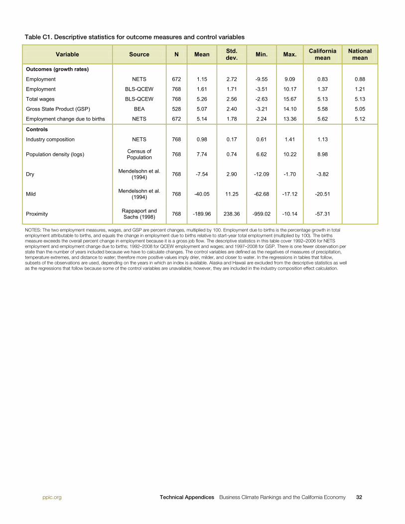
http://www.ppic.org/main/home.asp Technical Appendices Business Climate Rankings and the California Economy 32
Table C1. Descriptive statistics for outcome measures and control variables
Variable Source N Mean Std. dev. Min. Max. California
mean National
mean
Outcomes (growth rates) Employment NETS 672 1.15 2.72 -9.55 9.09 0.83 0.88
Employment BLS-QCEW 768 1.61 1.71 -3.51 10.17 1.37 1.21
Total wages BLS-QCEW 768 5.26 2.56 -2.63 15.67 5.13 5.13
Gross State Product (GSP) BEA 528 5.07 2.40 -3.21 14.10 5.58 5.05
Employment change due to births NETS 672 5.14 1.78 2.24 13.36 5.62 5.12
Controls Industry composition NETS 768 0.98 0.17 0.61 1.41 1.13
Population density (logs) Census of Population 768 7.74 0.74 6.62 10.22 8.98
Dry Mendelsohn et al. (1994) 768 -7.54 2.90 -12.09 -1.70 -3.82
Mild Mendelsohn et al. (1994) 768 -40.05 11.25 -62.68 -17.12 -20.51
Proximity Rappaport and Sachs (1998) 768 -189.96 238.36 -959.02 -10.14 -57.31
NOTES: The two employment measures, wages, and GSP are percent changes, multiplied by 100. Employment due to births is the percentage growth in total employment attributable to births, and equals the change in employment due to births relative to start-year total employment (multiplied by 100). The births measure exceeds the overall percent change in employment because it is a gross job flow. The descriptive statistics in this table cover 1992–2006 for NETS employment and employment change due to births; 1992–2008 for QCEW employment and wages; and 1997–2008 for GSP. There is one fewer observation per state than the number of years included because we have to calculate changes. The control variables are defined as the negatives of measures of precipitation, temperature extremes, and distance to water; therefore more positive values imply drier, milder, and closer to water. In the regressions in tables that follow, subsets of the observations are used, depending on the years in which an index is available. Alaska and Hawaii are excluded from the descriptive statistics as well as the regressions that follow because some of the control variables are unavailable; however, they are included in the industry composition effect calculation.

http://www.ppic.org/main/home.asp Technical Appendices Business Climate Rankings and the California Economy 33
Table C2. Relationship between business climate indexes and state controls, 1992–2008
SNEI DRCS-P DRCS-DC DRCS-BV SCI SBTC SBSI CDBI EFI EFINA FPRCNG Industry composition
1.316 1.244 -0.131 -1.489 1.112 2.549 0.898 -0.531 0.647 -0.019 -0.446 (0.880) (0.833) (0.838) (0.597)** (0.876) (1.104)** (1.151) (0.741) (0.854) (1.035) (0.673)
Population density
0.783 0.120 0.695 0.820 0.108 -0.634 -0.370 -0.807 -0.820 -0.202 0.154 (0.231)*** (0.212) (0.206)*** (0.207)*** (0.234) (0.232)*** (0.245) (0.163)*** (0.211)*** (0.288) (0.148)
Dry -0.088 -0.004 -0.073 -0.021 -0.018 -0.029 -0.015 0.060 0.089 0.008 -0.011 (0.080) (0.048) (0.074) (0.057) (0.076) (0.078) (0.102) (0.066) (0.071) (0.090) (0.045)
Mild -0.011 -0.058 -0.046 0.006 -0.043 0.013 0.017 0.008 0.016 0.035 -0.002 (0.012) (0.010)*** (0.010)*** (0.010) (0.011)*** (0.013) (0.015) (0.010) (0.010) (0.013)** (0.007)
Proximity -0.0006 0.0009 -0.0007 -0.0004 -0.0006 -0.0010 -0.0006 -0.0003 -0.0006 -0.0003 -0.0007 (0.0007) (0.0007) (0.0007) (0.0009) (0.0008) (0.0009) (0.0011) (0.0006) (0.0010) (0.0010) (0.0004)*
N 48 48 48 48 48 48 48 48 48 48 48
R2 0.51 0.53 0.51 0.37 0.39 0.30 0.12 0.61 0.53 0.18 0.07
NOTES: The table shows estimated regressions of the averages of each business climate index across years on the state controls, which are time invariant.

http://www.ppic.org/main/home.asp Technical Appendices Business Climate Rankings and the California Economy 34
Appendix D: Detailed Findings
Economic Outcomes and Business Climate Regressions
We report how business climate indexes predict economic outcomes in Tables D1–D5. Each table covers one of our five economic outcomes and reports a set of regressions for each business climate index, in each column. First, we estimate the model with nothing but the business climate index and year fixed effects as independent variables, to get at the simple relationship between the indexes and state economic growth. In this case, the dependent variable is defined as the one-year percentage change. Second, we augment this model with the controls for the industry composition effect, population density, climate, and proximity to navigable water. We then repeat this last, augmented specification for two- and three-year percent changes (always annualized), also varying the window relative to the business climate index over which these changes are measured. Economic theory provides no guidance as to which of these specifications (after the first) is correct. Instead, our goal is to estimate a variety of reasonable specifications, to see whether we identify indexes that have robust relationships with economic outcomes. In our discussion, we focus on the one-year outcome changes, in order to explain our approach and findings, but we include a table summarizing our results for all specifications and weigh them equally in reaching our conclusions.
Given that our goal is to assess how well business climate indexes predict economic growth, the ideal way to identify informative business climate indexes would be to estimate relationships between business climate indexes and economic outcomes over a long sample period, and then test the ability of business climate indexes to forecast economic outcomes out of sample. However, given the relatively short sample period available to us, especially for some of the indexes, this is infeasible. Our conclusions have to be interpreted, then, keeping in mind the caveat that going forward the relationships between business climate indexes and economic outcomes may be weaker than is suggested by our in-sample estimates.
Tables D1 and D2 report results for employment growth as measured by the NETS and the QCEW, respectively. In Table D1, for many of the indexes (SNEI, DRCS-P, DRCS-BV, SCI, and FPRCNG), the estimated relationship between the index and NETS employment growth is never statistically significant. For these indexes, the estimates are typically small and vary in sign, with a central tendency of about zero. With regard to the magnitude, for the SNEI index, for example, the estimated coefficient of −0.032 means that a one-standard deviation increase in this index is associated with employment growth that is lower by a trivial three-hundredths of a percentage point. To provide a better understanding of what this magnitude means, the number in square brackets reports the change in the percentage rate of growth of employment that is associated with a move in the rankings from the 40th to the 10th state, using the average values of the index for the included years—what would be considered a very substantial “jump up” in the rankings. In this example, the estimate is −0.061, implying a tiny decline in employment growth (consistent with the negative coefficient estimate). Clearly, then, these indexes have essentially no predictive power for employment growth as measured by the NETS. We would also add the CDBI index to this list, for which there is a significant estimated effect only for the first specification with no controls, and the effect is also very small once controls are added. And for the DRCS-DC index, there is an anomalous estimated negative effect that is significant in some cases.

http://www.ppic.org/main/home.asp Technical Appendices Business Climate Rankings and the California Economy 35
Intermediate cases are the SBTC, SBSI, and EFI indexes, for which the estimated coefficient of the index is significant and positive for at least one specification with the full set of controls included, and for which the estimates are often larger in magnitude. The strongest and most robust evidence, however, is for the EFINA index: we find positive, more sizable estimates for every specification, and the estimates are statistically significant in every case.1 The magnitudes with controls are centered on 0.16 to 0.18. To interpret the magnitudes, taking the last estimate of 0.180 for the EFINA index implies that moving a state from the 40th to the 10th place in the rankings would increase the rate of growth of employment by 0.317 percentage point—i.e., three-tenths of a percentage point faster employment growth. This can be compared with the mean employment growth rate of 1.15 percent reported in Table C1, implying faster growth by 28%.
Note that the table (and the similar tables that follow) divides the results (with thick vertical lines) for the different “clusters” of indexes discussed earlier; to reiterate, the first five constitute the productivity cluster, and the next five the taxes-and-costs cluster. Interestingly, of the indexes for which there is at least some persistent evidence of a positive relationship between the index and employment growth, all are in the taxes-and-costs cluster. Conversely, none of the indexes in the productivity clusters has a positive relationship with employment growth. Thus, the principal result that emerges is that states ranked better on the tax-and-cost-focused indexes—meaning lower taxes, regulatory costs, etc.—have faster employment growth.
It is also worth noting some of the results for the control variables; these are similar for the different specifications, and hence are only shown for one specification. In particular, the estimated coefficients of the industry composition effect variable are more or less centered on one. Population density is almost always negatively associated with employment growth (except in one specification), and the estimate is generally statistically significant. This presumably reflects the higher growth rate associated with a lower base, more room to expand, lower land costs, and so on, offsetting any agglomeration effects that might be in the opposite direction. The “dry” variable, meaning less precipitation, is always estimated to be positively associated with employment growth, although the estimate is never statistically significant. In contrast, there is a strong positive association between a mild climate and employment growth. The estimate is strongly statistically significant in every specification. Moreover, the implied effect is large. In this case moving from the 40th to the 10th position in the rankings is associated with a rate of growth of employment that is higher by about 0.55 to 1.05 percentage points—much larger than the estimated association with even the “strongest” business climate index. Somewhat surprisingly, perhaps, the estimated effect of proximity to navigable water is negative, and sometimes statistically significant, and the implied magnitude shown in square brackets is sometimes large (about −0.3 in some cases). This is not the usual predicted effect from models of economic geography, but may reflect that shifts in recent decades towards services and low weight-to-value products have made proximity to water relatively less important, and that the expansion in these sectors has been easier in places not tied to the older industries for which this proximity was important.
Finally, for the business climate indexes for which we find at least some evidence suggesting positive effects of a good business climate (SBTC, SBSI, EFI, and EFINA most of all), the inclusion of the control variables generally reduces the magnitude of association with the business climate index substantially—by half for EFINA and SBSI and roughly one-third for SBTC (though not at all for EFI)—and often reduces the level of
1 This may be partly because, relative to most of the other indexes in the taxes-and-costs cluster, the EFINA index is available for more years (see Table A1).

http://www.ppic.org/main/home.asp Technical Appendices Business Climate Rankings and the California Economy 36
statistical significance. The same is also true for the other index for which the simple specification in the first row suggests a significant (albeit negative) effect (DRCS-DC). Thus, a good deal of the association between business climate indexes and employment growth—an association that in almost every case suggests that a higher business climate ranking implies faster growth—is partly and sometimes substantially mediated by the other control variables. To some extent, then, states with apparently “good” business climate rankings tend to have other advantages relative to other states, such as milder weather and lower population density. Nonetheless, Table D1 still shows that a relationship between employment growth and taxes and costs—as captured by at least some of the business climate indexes—persists once the control variables are taken into account.
Table D2 repeats the analysis of Table D1, but using employment growth as measured by the QCEW. As it turns out, the evidence is very similar. There is essentially no evidence linking the business climate indexes related to productivity to QCEW employment growth, whereas there is more evidence—indeed, perhaps more so than in Table D1—linking lower taxes and costs to employment growth. All five indexes in the taxes-and-costs cluster have coefficients implying that a move from a 40th to 10th ranking is associated with a 0.2 to 0.4 percentage point increase in employment growth; the estimates are near the high end of that range for the two indexes showing a statistically significant relationship with employment growth (SBTC and EFINA). And similar conclusions regarding the mediating effects of the other controls apply here as well.
In Tables D3 and D4, we turn to two alternative measures of economic growth: growth of total wages, and of GSP. For both measures, our main findings are similar to those for employment growth, though somewhat less strong. None of the indexes in the productivity cluster has a positive, statistically significant relationship with either outcome when we include controls; only SNEI and only in the wage growth regression has a positive relationship—at the 10% significance level—without control variables. The DRCS-BV index even has a negative, large, and statistically significant relationship with wage and GSP growth when controls are included, as this index also did—to a lesser extent—for QCEW employment growth. In the taxes-and-costs cluster, four of the five indexes have a large, positive, statistically significant relationship with wage and GSP growth without controls. However, with controls only the EFINA index has a persistent positive and significant estimated effect on these outcomes; there are, though, some significant positive estimates for the SBTC and CDBI indexes. The estimated magnitudes drop by modest amounts in the wage growth regression and by nearly half in the GSP growth regression when the controls are added. As in the employment growth regressions, mild climate, the industry composition effect, and lower population density are positively associated with wage and GSP growth.
We next consider employment change in new establishments—“births”—as an outcome variable, for several reasons. Births represent a large share of job creation (Kolko and Neumark, 2007), and California’s economy exhibits more employment growth from births than the national average (see Table C1). Studying this dimension of job growth also responds to a general and long-standing policy focus on the importance of small businesses in job creation—with entrepreneurship and business creation often explicit policy goals—as well as more recent research indicating that job growth in the small business sector is largely dependent on new small businesses (Haltiwanger et al., 2009).2 Table D5 shows that the productivity indexes predict
2 We purposely exclude business relocation as an indicator of economic growth. Neumark et al. (2005, 2007) and Kolko and Neumark (2007) show that measures of businesses leaving California—which are often cited in critiques of the state’s business climate—offer a narrow and for the most part meaningless view of the state’s economic situation. California’s net employment change due to relocation is trivial relative to the size of the economy. We focus instead on economic growth measures that reflect overall economic activity, including but encompassing much more than employment changes due to relocation.
http://www.ppic.org/main/home.asp Technical Appendices Business Climate Rankings and the California Economy 37
employment change due to births at least as well as the taxes-and-costs cluster, when controls are included; this result is the opposite of what we find for overall employment, wage, and GSP growth. Four of five of the productivity indexes (SNEI, DRCS-P, DRCS-DC, and DRCS-BC) have a positive, statistically significant relationship (at the 10% level) with employment change due to births in the models with changes defined over one, two, and three years; several of the cost-based indexes do as well, and the EFI coefficients are larger than those of the productivity indexes or the other taxes-and-costs indexes.3
We emphasize our results on overall growth in employment, wages, and GSP. It is unclear whether, from a policy perspective, greater employment growth due to births in the absence of greater net employment growth (which implies greater excess job reallocation) is desirable. It may be that greater employment growth due to births in the absence of contemporaneous faster net employment growth leads to higher long-term economic growth, if new firms take advantage of newer technologies and processes that allow them to generate longer-term growth.4 We found no evidence that the productivity indexes are associated with later economic growth, though only within our time period of 1992–2008.5
Table D6 summarizes these results for all eleven indexes, five outcomes, and five specifications shown in Tables D1–D5. For both employment outcomes, the taxes-and-costs business climate indexes have a positive and statistically significant estimated effect in nearly half of the specifications we test (11 out of 25). However, among the indexes in this cluster, effects vary. The EFINA index has a statistically significant relationship with both employment outcome measures in every specification we test (five out of five), as does SBTC for the QCEW employment outcome; in contrast, CDBI never has a significant relationship with employment growth in any specification, and for NETS employment the estimate is always negative. For wages, EFINA has a significant positive coefficient in all five specifications, and SBTC does in three out of five, though the other three taxes-and-costs indexes are never significant for wages. For GSP growth, EFINA is significant in three out of five specifications, CDBI in one, and the others in none. For indexes and outcomes that are significant over most or all five specifications, the coefficient estimates tend to cluster in a tight range, such as 0.160-0.183 for EFINA in the NETS employment growth regressions.
Among the productivity indexes, the average magnitude is either negative or insignificant (NETS employment, wages, and GSP), or slightly positive or insignificant in the positive direction (QCEW employment). For employment change due to births, the productivity indexes have positive coefficients in every instance and are statistically significant in 20 out of 25 specifications, the most robust relationship between a cluster and an outcome in Table D6.
We subjected these results to several sensitivity tests.6 First, because indexes in the productivity cluster each include components that we consider to be outcomes rather than factors that affect outcomes, we recalculated
3 Employment change due to births is, of course, a component of overall net employment growth; for the productivity indexes to be associated with employment change due to births but not with overall employment change, these indexes must also be (positively) associated with one or more component of gross job destruction—deaths, contractions, or moves-out—or negatively associated with the other components of gross job creation—expansions and moves in. We confirmed (tables available upon request) that most of the productivity indexes are positively associated with components of gross job creation and gross job destruction. 4 This could be a reflection of the “creative destruction” emphasized by Schumpeter (1942). 5 Dividing our years into two time periods and regressing later growth on both earlier and later versions of the indexes revealed no patterns that might suggest productivity indexes are associated with future growth (results available on request). However, nearly all index rankings are quite stable over time, making it hard to separate contemporaneous from lagged effects of the indexes (Table A3). Moreover, the absence of a longer time-series makes it difficult to draw strong conclusions about whether factors that contribute to more births also contribute to growth in the longer run. 6 In addition to the analyses described next, we also re-ran our baseline models including state fixed effects. As expected from the high correlation of business climate indexes for states over time, standard errors increased considerably, and almost no coefficients of the indexes

http://www.ppic.org/main/home.asp Technical Appendices Business Climate Rankings and the California Economy 38
these indexes and generated modified indexes stripped of outcome components.7 Our regression results changed little with these modified indexes.8
Second, we repeated the regressions for the taxes-and-costs cluster adding a control for the DRCS-BV index, the only index from the productivity cluster that generally has a statistically significant (albeit negative) relationship with our growth outcomes in the regression models with the control variables included. Although we know from Table A3 that indexes in different clusters have no statistically significant positive correlation, some pairs—like CDBI and DRCS-BV—exhibit significant and large negative correlations, raising the possibility that we are misattributing the effects of an index to those in another cluster when we include each index singly in Tables D1–D5.9 With few exceptions, the taxes-and-costs index coefficients changed little when the DRCS-BV index is included as a control.
Finally, we included doctorate degrees granted per capita as an additional control. The presence of research universities is a policy variable whose effect on economic growth might only be apparent in the long-term, as the economic development impact of universities often comes through the incubation of new industries. Doctorate degrees granted per capita is a measure of the presence, size, and emphasis on graduate training of research universities. Other aspects of the higher-education system, like community colleges, could better reflect the relationship between higher education and economic growth, but our reason for including this control is to test the robustness of the business climate index findings, not to draw conclusions about the complicated relationship between education and growth. The inclusion of this variable had little effect on the business climate index coefficients, and the relationship between the doctorate degrees variable and economic growth was typically negative and sometimes significant.10 We did not test measures of educational attainment—such as the share of adults with a college degree—as control variables because educational attainment is already included in some of the productivity-focused business climate indexes.
We explored two possibilities for heterogeneous effects. First, we found that the relationship between business climate indexes and economic performance is similar in years when the national economy grew faster and in years when the national economy grew more slowly.11 Thus, a poor business climate does not appear to harm states more in recessions than in regular times, but rather slows growth throughout the business cycle. Second, we found that the relationship between the business climate and economic
were statistically significant. More specifically, for the taxes-and-costs indexes, the coefficient estimates were often little changed, but the standard errors were so much larger that these estimated coefficients were no longer statistically significant. We therefore interpret these fixed-effects results as providing no additional insight while at the same time not contradicting our baseline results. (Results available upon request.) 7 As shown in Table A2, some indexes include components better interpreted as economic outcomes than as pre-existing conditions that shape these outcomes. Examples are: the employment growth measures, unemployment rate, involuntary part-time employment, and pay measures in the DRCS-P index; initial public offerings and “gazelle” jobs in the SNEI; new companies, business closings, and job growth due to new businesses in the DRCS-BV index; and labor force participation (% of adults in the labor force) in the SCI index. Admittedly, the list of potentially problematic components could be extended, as cost factors such as rents, higher tax revenues and government spending, and lower tax rates could reflect the impact of economic activity rather than prior policy choices. However, we focus on those that are clear outcomes that do not directly reflect policy choices. We were able to generate the SNEI and the three DRCS indexes omitting the outcome components. 8 We would have expected any positive relationships between our economic outcomes and indexes containing outcomes to diminish when stripping out the outcome components, but the indexes that incorporate outcome components were in the productivity cluster and generally showed no positive relationship with net employment growth, wages, or GSP in the first place. 9 Results available on request. Because of the strong positive correlation between indexes within each cluster, we do not attempt to enter all indexes as independent variables in a single regression. Also, because each index is available for different years in the time period we study, we would have too few years of observations if we restricted ourselves to years when multiple indexes were available. 10 Results available on request. 11 We tested this two ways. First, we added an interaction between the business climate index and the national value for the dependent variable to our baseline regressions with controls in Tables D1-D5. Second, we divided our sample years in half based on whether national GDP growth was above or below the median annual national growth for the time period and repeated our baseline regressions for each sub-sample of years. Results available on request.

http://www.ppic.org/main/home.asp Technical Appendices Business Climate Rankings and the California Economy 39
performance is similar in states with a good deal of economic activity near a state border, like New Hampshire or Maryland, and in states with most economic activity far from state borders, like California or Texas. Even though almost no business in California or Texas could move across the state line and stay within the same local labor market, economic performance in these states is as sensitive to the business climate as in states where many businesses are near another state’s border.12
Our last extension was to look at economic outcomes in sectors we hypothesize could be more sensitive to differences in state business climates. Kolko and Neumark (2007) identify some sectors as more “footloose” than others, based on gross job creation and destruction due to relocation into and out of California. Intuitively, industries that serve a national or international market should be more footloose than those tied to local markets (such as services delivered in-person, like haircuts, or retailers) or dependent on local natural resources or features (like mining, forestry, or shipping). The most footloose sectors are manufacturing (NAICS 31-33), information (51), finance and insurance (52), and professional and technical services (54). We repeat our regression models for manufacturing only and for information, finance and insurance, and professional and technical services together. We look separately at manufacturing because, unlike the other three sectors, it has long had a declining share of employment, has traditionally provided reasonably high-paying jobs for middle-class workers, and is often the target of specific tax credits and economic development efforts. We look at private sector employment and wages in these industries from the QCEW. For purposes of comparison, the first row of each panel of Table D7 reports results for all industries, restricting the data to the private sector.
For QCEW employment and wages, the relationship between business climate indexes in the taxes-and-costs cluster and growth is stronger for manufacturing than for overall employment. The top panel of Table D7 shows that the coefficients on three indexes—SBTC, SBSI, and CDBI—are at least twice as large for manufacturing (second row) as overall private-sector employment (first row), and the SBSI and CDBI coefficients become statistically significant for manufacturing. Comparing overall private-sector employment with the three footloose non-manufacturing sectors (third row), no clear pattern emerges: coefficient magnitudes are similar, and two of the five indexes are statistically significant for footloose employment and overall private sector employment, compared with four for manufacturing employment. The results for wage growth in the bottom panel of Table D7 are broadly similar. The relationship between the taxes-and-costs indexes is stronger for manufacturing wage growth than for wage growth in the private sector overall or in the three footloose non-manufacturing sectors. The same three indexes noted above—SBTC, SBSI, and CDBI—have larger coefficients and are statistically significant for manufacturing wage growth only.
Looking at the effect of the productivity indexes on these same sectors, there is still no consistent relationship with economic growth. Comparing the effect on manufacturing employment (QCEW) with the effect on overall private sector employment in Table D7 (top panel), the coefficients on SNEI, DRCS-P, DRCS-DC, and DRCS-BV all become larger in the negative direction, though only one—DRCS-BV—has a statistically significant negative estimated effect on manufacturing employment. Comparing the estimated effect on employment in the footloose non-manufacturing sectors with the estimated effect on overall private sector employment, there is little change except that SNEI is positive and significant at the 10% level. Looking at the productivity indexes and wage growth in Table D7 (bottom panel), there are no big differences between
12 We included an interaction between the share of workers that commute daily across state lines in either direction and the business climate index (as well as the main effect of this cross-commuting measure) in our baseline regressions with controls in Tables D1–D5. Results available on request.

http://www.ppic.org/main/home.asp Technical Appendices Business Climate Rankings and the California Economy 40
the results for manufacturing and the private sector overall, while for footloose non-manufacturing sectors SNEI becomes more strongly positive and DRCS-BV is still negative but no longer statistically significant. The stronger predictive power that SNEI has for QCEW employment and, even more so, for wages may be due to the overlap between SNEI’s heavy emphasis on indicators relevant for technology and related industries (see Table A2) and our definition of “footloose industries,” which includes the information sector and other technology industries. These SNEI results highlight that business climate measures geared toward specific industries may predict outcomes in those industries better than they predict outcomes for the economy overall.13
The main conclusions that emerge from these business climate index regressions are: (1) indexes focusing on taxes and costs of doing business have some predictive power for economic growth, especially for manufacturing wage and employment growth, while productivity-focused indexes do not; and (2) productivity-focused indexes predict births, though not economic growth.
California’s Economic Performance and the Business Climate
One question motivating this research is why California’s economic performance is at or above the national average even though its business climate rankings are quite poor on the taxes-and-costs cluster, while middling or favorable on indexes in the productivity cluster. The answer does not appear to be that indexes in the productivity cluster capture factors that are more important for economic growth than do the taxes-and-costs cluster. Although California’s middling-to-favorable rankings on indexes in the productivity cluster correspond better to California’s middle-to-good economic performance than do California’s poor rankings on indexes in the taxes-and-costs cluster, we have shown that only the taxes-and-costs cluster predicts employment, wage, or GSP growth. In this section, we assess why California’s growth outperforms its rankings on indexes in the taxes-and-costs cluster, interpreting the estimated effects from the analysis of the taxes-and-costs indexes as capturing the causal effects of the policies the indexes capture.
California’s economic growth is higher, in relative terms, than its ranking on the taxes-and-costs business climate indexes alone would predict. In fact, California is near or above the national average for all four economic growth measures, as shown in Table C1. Figure D1, top panel, plots the average ranking across the five business climate indexes in the taxes-and-costs cluster against annualized QCEW employment change: California’s average ranking is the lowest aside from New York, but its average employment growth is above the fitted line and also above that of many other states. 14
California’s economic performance is better than would be expected given its poor business climate because it has other characteristics—captured in the control variables—that are particularly favorable to economic growth. To measure and compare the contributions of the taxes-and-costs business climate indexes and the control variables to economic growth in California and other states, we multiply the regression coefficients by the states’ index values and values for the control variables. For each index we calculate the estimated contribution of the business climate index to QCEW employment growth, �̂��𝐵𝐶𝑖 − 𝐵𝐶� and the estimated total contribution of the five non-policy factors to employment growth �𝑋𝑖 − 𝑋��̂�, where �̂� and �̂� are from 13 These positive results for SNEI persisted even when we used the modified version of the index that excluded outcome components, as described above. 14 The corresponding figure for the productivity cluster (Figure D1, lower panel) shows no statistical relationship between the productivity cluster scores and employment growth: the fitted line is essentially flat.

http://www.ppic.org/main/home.asp Technical Appendices Business Climate Rankings and the California Economy 41
Table D2 (for QCEW employment growth). Averaging over the models for the three indexes with consistent relationships with economic growth—SBTC, EFI, and EFINA—yields two measures for each state: the estimated contribution of the business climate to employment growth, and the estimated contribution of the five non-policy factors to employment growth. Figure D2 plots these for all states.
Figure 2 in the main text shows that California’s values for our control variables—notably its mild climate—appear to make positive contributions to economic growth, larger in magnitude than the negative contribution of its rankings on these three business climate indexes. Figure D2 shows that California is unique among large states in having these offsetting influences. Among the states for which the average across the SBTC, EFI, and EFINA indexes make a larger negative contribution to growth, such as New York, all have factors outside the control of policy that together contribute negatively to employment growth—unlike California. In fact, the only states, like California, where these business climate indexes make a negative contribution to economic growth and factors beyond policy control make a positive contribution to growth are New Mexico, Montana, and Idaho—all states with much smaller populations and economies than California.
Many states have both a favorable business climate and favorable non-policy factors, such as Nevada, Colorado, Arizona, Wyoming, and Texas; many states are unfavorable on both dimensions, like New York, Rhode Island, and New Jersey. For both these sets of states, ignoring non-policy factors could lead to giving the business climate undue credit (or blame) for high (or low) employment growth since the non-policy factors contribute to employment growth in the same direction as the business climate does. In a few states, the business climate and non-policy factors have offsetting estimated effects on employment growth. Although harder to see in the figure, Indiana, Tennessee, and several other mostly Southern states have favorable business climates yet unfavorable non-policy factors—the opposite of the offsetting effects in California.
The implication is that some of California’s natural advantages—particularly its dry, mild climate—offset the disadvantages of policies that give the state such poor rankings on the taxes-and-costs business climate indexes.
Policy and Economic Performance: Which Taxes and Costs Matter?
We focus on business climate indexes, rather than the individual components that constitute them, for two reasons. First, the indexes themselves are a large part of the public debate and receive political and media attention; thus, it is useful to assess directly their predictive power. As important, though, the indexes all represent attempts to reduce the innumerable policy and other variables that could affect economic performance down to a single measure. With far more potential individual components than there are observations on states and years of data, some method of data reduction is essential. Since existing research has demonstrated that the effects of individual components are quite sensitive to the other components included in a model, we are reluctant to make arbitrary decisions about which few components from the universe of possibilities to include in a model testing individual policy variables. Any attempt to look at a limited number of individual policy variables risks omitted variable bias, particularly if policy variables are highly correlated with each other. Unless a comprehensive set of policy variables is included in a model—which is precluded by limited degrees of freedom and the high correlation among many policy variables—the results from a model with limited policy variables could either mean that the included policies

http://www.ppic.org/main/home.asp Technical Appendices Business Climate Rankings and the California Economy 42
themselves matter for economic growth or that the included policies are proxies for related, omitted policies that matter.
Nonetheless, we are interested in trying to delve deeper into the business climate indexes that appear to matter to see whether we can say something more specific about the policies that might be most important to state economic growth. To do so, without ending up with the insurmountable problem of using individual policy variables, we use sub-indexes that constitute three of the indexes in the taxes-and-costs cluster—SBTC, EFINA, and EFI—and four of the indexes in the productivity cluster—SNEI and the three DRCS indexes. Within the taxes-and-costs cluster, only those three indexes organize the individual components into sub-indexes and report state scores for them. Fortunately, these three include the two indexes with the strongest positive relationship with economic growth (SBTC and EFINA). The third, EFI, includes a relatively wide range of taxes-and-costs components and therefore includes sub-indexes for regulation and litigation, which SBTC and EFINA lack (see Table A6a and the discussion in Appendix A). Together, the 13 sub-indexes in these three indexes include at least one of each of the five taxes-and-costs sub-categories that we defined in comparing the indexes in Table 2 and the sub-indexes in Table A6a. Within the productivity cluster, the SCI index presents ranks, not scores, for many years, and its sub-index definitions change over time, making these sub-indexes a challenge to incorporate into our models. Among the other four productivity indexes, the sub-indexes also span the sub-categories we defined in Table 2 and, for these sub-indexes, in Table A6b. Replacing the business climate indexes with sub-indexes in our empirical models lets us focus on narrower policy categories and their relationships with growth while taking into account the full range of components, without the limitations or arbitrariness introduced by including individual policies.
The regressions with one sub-index at a time are useful for comparing results across indexes: similar sub-indexes in different indexes, like EFINA-SG and EFI-WS, might have similar effects when looked at singly but different effects when controlling for the different set of sub-indexes each index includes. However, sub-indexes within an index are often highly correlated. Therefore, we first present regressions with one sub-index at a time, followed by regressions with all sub-indexes for a single index simultaneously. In all the sub-index regressions, we follow the same strategy that we use for indexes: we investigate five economic outcomes, present results using the same set of controls as before, and include year fixed effects and state-level control variables. As before, we report the implied effect of moving from 40th to 10th in the ranking on the sub-index; we focus on the four outcomes that most strongly reflect economic growth: employment from two data sources, wages, and GSP; and we present the specification with the one-year outcome change and then summarize the results from all specifications.
For the productivity sub-indexes, an additional complication is that many variables are themselves economic outcomes rather than factors potentially affecting economic outcomes. Sub-indexes including outcome variables could have a relationship with economic outcome measures by construction. Table A5 shows the portion of each sub-index that is outcomes. In our preferred specification, we omit three sub-indexes comprised 80% or more of outcome variables: the DRCS-P employment sub-index, the DRCS-P earnings and job quality sub-index, and the DRCS-BV entrepreneurial energy sub-index. For other sub-indexes with outcome variables—which account for at most one-third of each sub-index—we re-calculate the sub-indexes omitting the outcome variables, as we did for the overall productivity indexes above. We use these “stripped” sub-indexes in our sub-index regressions.
Including sub-indexes separately in our model (Table D8), one stands out for each of the three taxes-and-costs indexes. Among the five sub-indexes of SBTC, all of which measure different aspects of taxation, the

http://www.ppic.org/main/home.asp Technical Appendices Business Climate Rankings and the California Economy 43
corporate income tax index has a positive and statistically significant relationship at the 5% level with both employment growth measures, and with wage and GSP growth. For wages and GSP, the coefficient on the corporate tax sub-index is especially large relative to other sub-indexes. The individual income tax sub-index is positive, statistically significant, and of similar magnitude to the corporate tax sub-index for QCEW employment growth when scaled to the 40th–10th ranking difference; in no other instance is there a positive, significant relationship between an SBTC sub-index and an economic growth outcome measure. Note that the sub-indexes, like the indexes, are all scaled so positive values are intended to reflect a “better” business climate, according to the intent of the index.
The SBTC corporate tax sub-index captures numerous aspects of the corporate tax rate structure and base, such as the top marginal rate (higher results in a worse sub-index score); the number of tax brackets and their income thresholds (flatter is better); the generosity of the net operating loss deduction (more years and higher dollar limits are better); the extent of tax credits (fewer are better); and similarity with the federal tax code (conformity is better).
Unlike the SBTC index, the EFI and EFINA indexes include sub-indexes that span multiple categories of taxes and costs. Among the sub-indexes of EFINA, one sub-index—“size of government”—has a positive and significant relationship with all of our economic growth outcomes, and, except for GSP growth, a notably larger coefficient estimate than other sub-indexes. The two other EFINA sub-indexes have positive coefficient estimates that are significant for some outcomes and not others. Among the EFI sub-indexes, again one sub-index—“welfare spending”—stands out; this sub-index has a statistically significant relationship with all outcomes except GSP growth and the largest coefficient estimate among the EFI sub-indexes for all outcomes except wage growth. It is striking that the EFI and EFINA sub-indexes that stand out comprise similar policy measures: despite their different names (EFINA’s “size of government” sub-index and EFI’s “welfare-spending” sub-index), our analysis of their components revealed them both to consist primarily of variables describing the composition of government expenditure and, more specifically, the shares going to welfare and transfer payments (see Appendix A). In both cases, the larger these expenditures, the lower is economic growth. Again, note that the sub-indexes are scaled so that positive values are intended to reflect a “better” business climate, so higher values of these two sub-indexes correspond with lower welfare and transfer payments.
Given that the sub-indexes within an index are often fairly highly correlated, the independent estimated effects of a sub-index could appear different if we condition on the other sub-indexes, although it may also be difficult to identify the separate coefficients of multiple sub-indexes. We repeat our analysis by including all sub-indexes in a given index in the same model, reporting these results in Table D9. For SBTC, the corporate income tax sub-index coefficient estimates change little from the single sub-index model in Table D8, though the standard errors rise notably for this and the individual income tax sub-index; among the sub-indexes within the SBTC index, these two are the only highly correlated ones, so this is not surprising. Nonetheless, the corporate income tax sub-index continues to have a positive, statistically significant relationship with wage and GSP growth, but no longer with employment growth. The positive relationship we observe between the sub-index and growth does not appear to be driven by the top marginal tax rate.

http://www.ppic.org/main/home.asp Technical Appendices Business Climate Rankings and the California Economy 44
Replacing the corporate tax sub-index with the top marginal rate, the latter variable has no statistically significant relationship with any of our economic growth measures.15
Among the EFINA and EFI sub-indexes, the two that stood out in Table D8 (EFINA-SG and EFI-WS) do so even more sharply once we include all sub-indexes for a given index in the same regression. Both EFINA-SG and EFI-WS are positive and significant at the 10% level or less for three of our four main economic growth outcomes, and no other sub-index in either EFINA or EFI has a significant estimated effect for any of these outcomes, though EFI-SG is significant at the 5% level for employment growth due to births. The coefficient estimates on both of these sub-indexes became larger for most outcomes.
These results are quite robust to our alternative specifications for different time periods of the outcome variable. Table D10 uses the same format as Table D6, summarizing the results for each sub-index and outcome across our five specifications. The SBTC corporate tax sub-index is positive and statistically significant, with a very narrow range of coefficient estimates, in all five specifications for wage growth and GSP growth.16 The EFINA-SG sub-index is statistically significant in all five specifications for NETS employment, QCEW employment, and wages, again with a relatively narrow range of coefficient estimates, and the EFI-WS is significant for three of five specifications for QCEW employment, three for wages, and four for GSP.17 To provide a simpler view of the results, Table D11 presents a qualitative summary of the evidence.
These sub-index results are, in general, stronger and more robust than the results for the business climate indexes overall, as a comparison of the summary of index results in Table D6 and the summary of sub-index results in Table D10 shows. For each of the three indexes for which we could examine sub-indexes, one sub-index appears to account for most or all of the relationship between the index and economic growth outcomes, and in some cases a sub-index has a strong association with economic growth even though the index it belongs to does not. For instance, EFI has a positive, significant relationship with economic growth (excluding births) in only three out of 20 specifications (Table D6), though EFI’s welfare-spending sub-index has a positive, significant relationship with the economic growth measures in 11 out of 20 cases (Table D10) and larger coefficient estimates than for the overall index.18 EFI in particular is a broad index, covering many types of taxes and cost measures, and three of its five sub-indexes (fiscal, regulatory, and judicial) never have positive and significant relationships with any economic growth outcome.
15 This is true either without other sub-indexes (as in Table D8) or with other SBTC sub-indexes (as in Table D9). Moreover, when we include both the top marginal corporate tax rate and the corporate tax sub-index in the model in Table D9, the tax rate continues to have no relatationship with any growth outcome, and the estimated coefficient of the corporate tax sub-index remains of similar magnitude and significance. Results available upon request. 16 We subjected the SBTC sub-indexes to an additional robustness test. Because SBTC only includes components for tax rates and tax burdens, the SBTC sub-index model tells us about tax base composition, which could be correlated with expenditure composition and therefore subject to omitted variable bias since the EFINA and EFI results suggest that expenditure composition matters for economic growth. We re-ran the model with all SBTC sub-indexes (Table D9) and added the EFINA-SG sub-index (which is available for many of the same years); this does not change the coefficient estimates or significance on the SBTC corporate income tax sub-index. Results available upon request. 17 The sub-indexes, unlike the taxes-and-cost indexes, did not differ markedly for manufacturing and footloose industries relative to the private sector overall. For EFINA-SG, the coefficients for both employment and wage growth in manufacturing were similar to the total private sector but with much higher standard errors and therefore not statistically significant, and the coefficients were somewhat lower for employment and wage growth in footloose industries. For EFI-WS, the coefficient for employment growth was lower for manufacturing and higher for footloose industries than for the private sector overall, but in neither case significant; the coefficient for wage growth was slightly higher for manufacturing and nearer to zero for footloose industries than for the private sector overall, but again in neither case significant. Results available upon request. 18 We continue to focus on the two employment growth measures (NETS and QCEW), wage growth, and GSP growth as our four main economic growth outcomes. A given index or sub-index has five specifications for each of these four outcomes, yielding 20 specifications to compare.

http://www.ppic.org/main/home.asp Technical Appendices Business Climate Rankings and the California Economy 45
Among the “stripped” productivity sub-indexes, none has a positive, statistically significant relationship with more than one of our outcome variables when included singly or with the other sub-indexes in the same index.19
As a sensitivity check for the taxes-and-costs sub-index results, we replicated Table D9 once for each of the five productivity indexes, including a different productivity index as a control and comparing against the original Table D9 modified to include only the years for which the productivity index was also available. This check accounts for the possibility that the productivity index is an omitted variable, correlated with taxes-and-costs sub-indexes and an economic growth measure. For only one combination of a sub-index (EFI-WS) and a productivity index (SNEI) does the inclusion of the productivity index change the positive relationship between the sub-index and outcomes, and furthermore this combination is for a single year of data since EFI and SNEI were simultaneously available only in 1999. (Results available on request.)
The sub-index analysis yields two main conclusions. The first is that, among taxes, the corporate income tax rate structure and base matter for wage and GSP growth, though not necessarily for employment growth. The SBTC is the only index whose sub-indexes distinguish different tax streams, so this finding comes entirely from that one index.
The second, more robust, conclusion is that greater government expenditure on welfare and transfer payments is associated with slower economic growth, as shown by the results for EFINA-SG on employment and wages and the results for EFI-WS on QCEW employment, wages, and GSP. These findings hold true across multiple specifications and when controlling for sub-indexes that reflect tax rates and the tax burden, other costs of doing business, and regulatory and judicial indicators. The strength of this result is reinforced by its consistency across two different business climate indexes, covering different years and different sub-indexes that serve as controls in our model. Admittedly, the EFINA-SG sub-index contains more than conventional welfare and transfer spending. But the EFI-WS sub-index focuses only on the latter, and the results for the EFI-WS sub-index are qualitatively similar (and in some ways stronger, and in particular predictive of GSP growth) than the results for the EFINA-SG sub-index.
There are a couple of potential issues that might raise cautions about these findings for the sub-indexes related to welfare and transfer payments. One is that there is some scope for reverse causality. Given that welfare and transfer payments may go up when economic growth is slower (as more people become eligible for payments or for higher payments), causality running from economic growth to higher welfare and transfer payments could in principle generate our results (or bias their strength). Moreover, the EFINA-SG sub-index defines these payments as a share of GSP (rather than relative to population, as in the EFI-WS sub-index). This generates even more possibility of this type of bias, as slow GSP growth can also feed directly into a higher share of payments relative to GSP. Thus, if this reverse causality were more important, we should find a stronger positive relationship with the welfare and transfer payment sub-indexes (a high value of the sub-index implies low payments) and economic growth for the EFINA-SG sub-index, and in particular for the GSP growth results for that sub-index. This is not, however, what we find. First, we also find significant effects in this direction for the EFI-WS sub-index. Most important, perhaps, we find significant effects for GSP growth for the EFI-WS sub-index but not the EFINA-SG sub-index, the opposite prediction from what we would expect if reverse causality from defining payments as a share of GSP were driving the results. Nonetheless, we cannot rule out the hypothesis that faster economic growth leads to lower welfare
19 Results available upon request.

http://www.ppic.org/main/home.asp Technical Appendices Business Climate Rankings and the California Economy 46
and transfer payments, which would generate a bias in the direction of a positive effect of sub-indexes that capture welfare and transfer payments on economic growth.
Second, the EFINA-SG sub-index includes a broader set of expenditures, including state retirement pensions. It could therefore be high for a state because the state has a large retirement population (for example, Florida), rather than because these payments change behavior and lead to lower economic growth. However, this concern is assuaged by the fact that the results are similar for the EFI-WS sub-index, which includes only state expenditures focused much more sharply on those directed towards the more conventionally thought-of “welfare” population (see Table A5).20
One other reason to be less concerned that our results are driven by reverse causality is that we use across-state rather than within-state variation to identify the effects of business climate indexes. This may offer some advantage in terms of avoid endogeneity bias, as we avoid relying on short-term changes in state economic conditions that could affect some of the policy variables. Indeed when we simply ran regressions paralleling those in Table D9 using the state averages (i.e., the between regression), the results were similar, although sometimes a little weaker. The results could be slightly weaker either because the averaging removed an endogenous shorter-term response of welfare and transfer payments to economic growth, or because the averaging obscured a short-term response of economic growth to exogenous policy change. Nonetheless, the robustness of the conclusions to using longer-term variation is reassuring.
Overall, these considerations make us more confident—but not definitive—in interpreting the combined evidence as identifying the effects of welfare and transfer spending on economic growth.
20 In addition, the large retiree population in a state like Florida consists of many migrants from other states, so the retirees would not likely be a source of high state retirement pension expenditures.

http://www.ppic.org/main/home.asp Technical Appendices Business Climate Rankings and the California Economy 47
Table D1. Regressions for NETS employment, 1992–2006 Period SNEI DRCS-P DRCS-DC DRCS-BV SCI SBTC SBSI CDBI EFI EFINA FPRCNG
Business climate index
1-year changes
-0.032 -0.126 -0.298 -0.193 -0.190 0.395 0.262 0.195 0.335 0.311 0.039 (0.103) (0.093) (0.113)** (0.123) (0.129) (0.120)*** (0.102)** (0.080)** (0.132)** (0.103)*** (0.108) [-0.061] [-0.241] [-0.578] [-0.351] [-0.327] [0.564] [0.471] [0.245] [0.577] [0.547] [0.082]
R2 0.87 0.45 0.47 0.46 0.52 0.46 0.76 0.50 0.71 0.73 0.62 N 96 192 192 192 240 96 480 192 96 672 264 Business climate index
1-year changes
-0.031 0.144 -0.194 -0.105 -0.136 0.232 0.130 -0.077 0.354 0.160 0.012 (0.106) (0.124) (0.117) (0.133) (0.155) (0.128)* (0.078) (0.124) (0.194)* (0.083)* (0.094) [-0.059] [0.276] [-0.376] [-0.191] [-0.234] [0.331] [0.234] [-0.097] [0.610] [0.281] [0.025]
Industry composition
2.066 0.880 0.954 0.894 1.305 0.704 1.700 1.321 2.007 1.405 1.811 (0.591)*** (1.039) (1.001) (1.032) (0.921) (1.174) (0.676)** (0.938) (0.979)** (0.694)** (0.779)**
[0.575] [0.245] [0.266] [0.249] [0.363] [0.196] [0.473] [0.368] [0.559] [0.391] [0.504] Population density
-0.342 -0.343 -0.166 -0.233 -0.331 -0.226 -0.421 -0.446 0.080 -0.425 -0.484 (0.161)** (0.187)* (0.184) (0.196) (0.159)** (0.297) (0.100)*** (0.209)** (0.205) (0.102)*** (0.132)***
[-0.524] [-0.525] [-0.254] [-0.357] [-0.507] [-0.346] [-0.645] [-0.683] [0.122] [-0.651] [-0.741] Dry 0.039 0.050 0.039 0.045 0.031 0.085 0.039 0.033 0.025 0.034 0.008 (0.048) (0.047) (0.046) (0.048) (0.043) (0.066) (0.038) (0.047) (0.060) (0.047) (0.052) [0.230] [0.294] [0.230] [0.265] [0.182] [0.500] [0.230] [0.194] [0.147] [0.200] [0.047] Mild 0.026 0.036 0.020 0.028 0.022 0.043 0.025 0.037 0.031 0.028 0.036 (0.007)*** (0.011)*** (0.010)** (0.008)*** (0.011)* (0.012)*** (0.006)*** (0.008)*** (0.011)*** (0.008)*** (0.009)*** [0.647] [0.895] [0.497] [0.696] [0.547] [1.069] [0.622] [0.920] [0.771] [0.696] [0.895] Proximity -0.0014 -0.0009 -0.0009 -0.0008 -0.0009 0.0001 -0.0007 -0.0011 -0.0002 -0.0011 -0.0017 (0.0004)*** (0.0007) (0.0005) (0.0005) (0.0005)* (0.0007) (0.0006) (0.0005)** (0.0007) (0.0006)* (0.0008)** [-0.375] [-0.236] [-0.222] [-0.211] [-0.247] [0.023] [-0.191] [-0.298] [-0.063] [-0.297] [-0.439] R2 0.90 0.51 0.51 0.51 0.58 0.53 0.79 0.59 0.76 0.77 0.69 N 96 192 192 192 240 96 480 192 96 672 264 Business climate index
2-year changes
-0.104 0.074 -0.178 -0.089 -0.100 0.128 0.143 -0.102 0.009 0.177 -0.006 (0.105) (0.106) (0.107) (0.106) (0.136) (0.132) (0.081)* (0.138) (0.160) (0.086)** (0.069) [-0.197] [0.142] [-0.345] [-0.162] [-0.172] [0.183] [0.257] [-0.128] [0.016] [0.311] [-0.013]
N 96 192 192 192 192 96 432 144 96 624 264 Business climate index
2-year changes
(shifted back one year)
0.030 0.091 -0.211 -0.110 -0.150 0.208 0.131 -0.022 0.260 0.183 -0.006 (0.094) (0.118) (0.122)* (0.131) (0.180) (0.128) (0.078) (0.127) (0.105)** (0.086)** (0.079) [0.057] [0.174] [-0.409] [-0.200] [-0.259] [0.297] [0.236] [-0.028] [0.448] [0.322] [-0.013]
N 96 192 192 192 240 96 480 192 96 624 264 Business climate index
3-year changes
-0.018 0.056 -0.161 -0.094 -0.088 0.159 0.141 -0.105 -0.148 0.177 0.026 (0.100) (0.107) (0.111) (0.090) (0.141) (0.121) (0.077)* (0.142) (0.301) (0.085)** (0.072) [-0.034] [0.107] [-0.312] [-0.171] [-0.152] [0.227] [0.254] [-0.132] [-0.255] [0.311] [0.054]
N 96 144 144 144 144 48 384 96 48 576 223 Business climate index
3-year changes
(shifted back one year)
-0.039 0.061 -0.196 -0.099 -0.155 0.147 0.147 -0.030 0.062 0.180 -0.012 (0.096) (0.100) (0.109)* (0.110) (0.163) (0.112) (0.079)* (0.125) (0.121) (0.086)** (0.067) [-0.074] [0.117] [-0380] [-0.180] [-0.267] [0.210] [0.264] [-0.038] [0.107] [0.317] [-0.025]
N 96 192 192 192 192 96 432 144 96 576 264
NOTES: See notes to Table C1. Business climate indexes are standardized by year. Unit of observation is the state and year. All models include year fixed effects. Standard errors clustered by state are below coefficient estimates. ***,**, and * indicate significance at the 1%, 5% or 10% level. The square brackets show the estimated coefficients multiplied by the difference between the 10th and 40th state rankings for each variable. Hawaii and Alaska are excluded. The specifications using as dependent variables changes over longer periods, as indicated in the second column, also include industry composition, population density, dry, mild, and proximity as controls. Population density is entered in logs. Note that sample sizes vary based on the years for which the index are available (see Table A1), and the years required to define the dependent variable over different intervals.
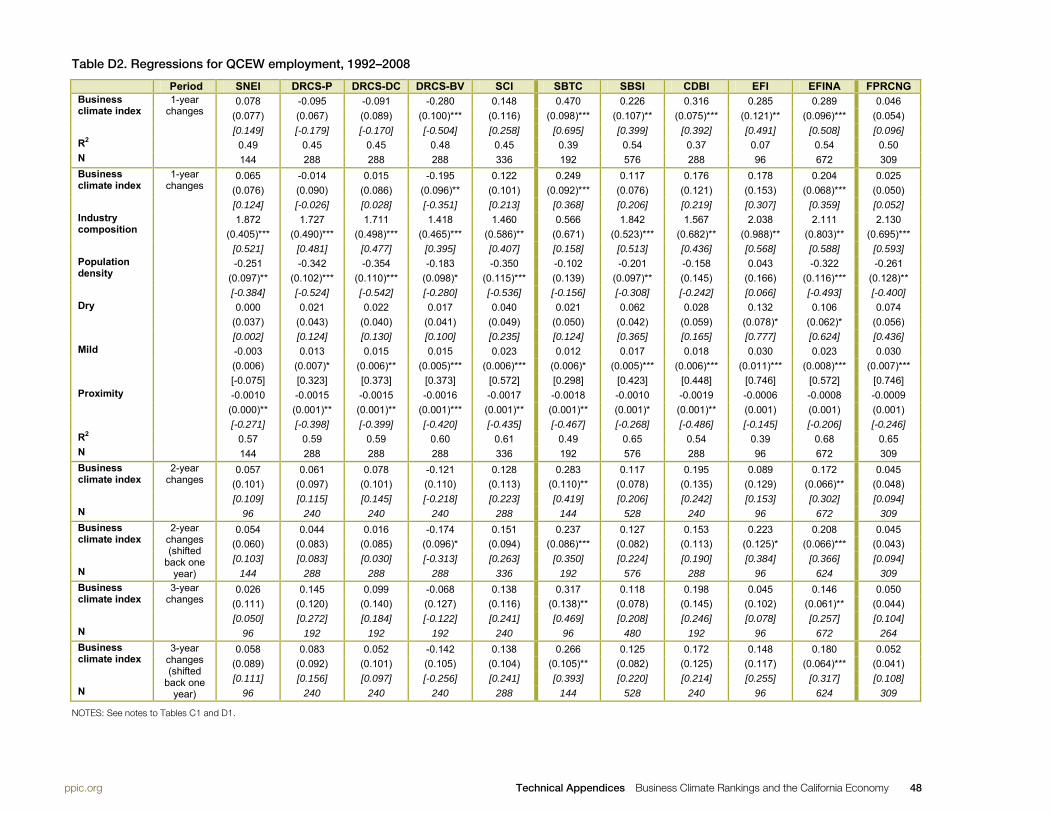
http://www.ppic.org/main/home.asp Technical Appendices Business Climate Rankings and the California Economy 48
Table D2. Regressions for QCEW employment, 1992–2008
Period SNEI DRCS-P DRCS-DC DRCS-BV SCI SBTC SBSI CDBI EFI EFINA FPRCNG Business climate index
1-year changes
0.078 -0.095 -0.091 -0.280 0.148 0.470 0.226 0.316 0.285 0.289 0.046 (0.077) (0.067) (0.089) (0.100)*** (0.116) (0.098)*** (0.107)** (0.075)*** (0.121)** (0.096)*** (0.054) [0.149] [-0.179] [-0.170] [-0.504] [0.258] [0.695] [0.399] [0.392] [0.491] [0.508] [0.096]
R2 0.49 0.45 0.45 0.48 0.45 0.39 0.54 0.37 0.07 0.54 0.50 N 144 288 288 288 336 192 576 288 96 672 309 Business climate index
1-year changes
0.065 -0.014 0.015 -0.195 0.122 0.249 0.117 0.176 0.178 0.204 0.025 (0.076) (0.090) (0.086) (0.096)** (0.101) (0.092)*** (0.076) (0.121) (0.153) (0.068)*** (0.050) [0.124] [-0.026] [0.028] [-0.351] [0.213] [0.368] [0.206] [0.219] [0.307] [0.359] [0.052]
Industry composition
1.872 1.727 1.711 1.418 1.460 0.566 1.842 1.567 2.038 2.111 2.130 (0.405)*** (0.490)*** (0.498)*** (0.465)*** (0.586)** (0.671) (0.523)*** (0.682)** (0.988)** (0.803)** (0.695)***
[0.521] [0.481] [0.477] [0.395] [0.407] [0.158] [0.513] [0.436] [0.568] [0.588] [0.593] Population density
-0.251 -0.342 -0.354 -0.183 -0.350 -0.102 -0.201 -0.158 0.043 -0.322 -0.261 (0.097)** (0.102)*** (0.110)*** (0.098)* (0.115)*** (0.139) (0.097)** (0.145) (0.166) (0.116)*** (0.128)**
[-0.384] [-0.524] [-0.542] [-0.280] [-0.536] [-0.156] [-0.308] [-0.242] [0.066] [-0.493] [-0.400] Dry 0.000 0.021 0.022 0.017 0.040 0.021 0.062 0.028 0.132 0.106 0.074 (0.037) (0.043) (0.040) (0.041) (0.049) (0.050) (0.042) (0.059) (0.078)* (0.062)* (0.056) [0.002] [0.124] [0.130] [0.100] [0.235] [0.124] [0.365] [0.165] [0.777] [0.624] [0.436] Mild -0.003 0.013 0.015 0.015 0.023 0.012 0.017 0.018 0.030 0.023 0.030 (0.006) (0.007)* (0.006)** (0.005)*** (0.006)*** (0.006)* (0.005)*** (0.006)*** (0.011)*** (0.008)*** (0.007)*** [-0.075] [0.323] [0.373] [0.373] [0.572] [0.298] [0.423] [0.448] [0.746] [0.572] [0.746] Proximity -0.0010 -0.0015 -0.0015 -0.0016 -0.0017 -0.0018 -0.0010 -0.0019 -0.0006 -0.0008 -0.0009 (0.000)** (0.001)** (0.001)** (0.001)*** (0.001)** (0.001)** (0.001)* (0.001)** (0.001) (0.001) (0.001) [-0.271] [-0.398] [-0.399] [-0.420] [-0.435] [-0.467] [-0.268] [-0.486] [-0.145] [-0.206] [-0.246] R2 0.57 0.59 0.59 0.60 0.61 0.49 0.65 0.54 0.39 0.68 0.65 N 144 288 288 288 336 192 576 288 96 672 309 Business climate index
2-year changes
0.057 0.061 0.078 -0.121 0.128 0.283 0.117 0.195 0.089 0.172 0.045 (0.101) (0.097) (0.101) (0.110) (0.113) (0.110)** (0.078) (0.135) (0.129) (0.066)** (0.048) [0.109] [0.115] [0.145] [-0.218] [0.223] [0.419] [0.206] [0.242] [0.153] [0.302] [0.094]
N 96 240 240 240 288 144 528 240 96 672 309 Business climate index
2-year changes (shifted
back one year)
0.054 0.044 0.016 -0.174 0.151 0.237 0.127 0.153 0.223 0.208 0.045 (0.060) (0.083) (0.085) (0.096)* (0.094) (0.086)*** (0.082) (0.113) (0.125)* (0.066)*** (0.043) [0.103] [0.083] [0.030] [-0.313] [0.263] [0.350] [0.224] [0.190] [0.384] [0.366] [0.094]
N 144 288 288 288 336 192 576 288 96 624 309 Business climate index
3-year changes
0.026 0.145 0.099 -0.068 0.138 0.317 0.118 0.198 0.045 0.146 0.050 (0.111) (0.120) (0.140) (0.127) (0.116) (0.138)** (0.078) (0.145) (0.102) (0.061)** (0.044) [0.050] [0.272] [0.184] [-0.122] [0.241] [0.469] [0.208] [0.246] [0.078] [0.257] [0.104]
N 96 192 192 192 240 96 480 192 96 672 264 Business climate index
3-year changes (shifted
back one year)
0.058 0.083 0.052 -0.142 0.138 0.266 0.125 0.172 0.148 0.180 0.052 (0.089) (0.092) (0.101) (0.105) (0.104) (0.105)** (0.082) (0.125) (0.117) (0.064)*** (0.041) [0.111] [0.156] [0.097] [-0.256] [0.241] [0.393] [0.220] [0.214] [0.255] [0.317] [0.108]
N 96 240 240 240 288 144 528 240 96 624 309
NOTES: See notes to Tables C1 and D1.

http://www.ppic.org/main/home.asp Technical Appendices Business Climate Rankings and the California Economy 49
Table D3. Regressions for QCEW wages, 1992–2008
Period SNEI DRCS-P DRCS-DC DRCS-BV SCI SBTC SBSI CDBI EFI EFINA FPRCNG Business climate index
1-year changes
0.256 -0.165 -0.253 -0.573 0.091 0.648 0.290 0.344 0.237 0.420 0.094 (0.141)* (0.097)* (0.116)** (0.155)*** (0.160) (0.221)*** (0.141)** (0.132)** (0.238) (0.109)*** (0.090) [0.489] [-0.310] [-0.471] [-1.032] [0.159] [0.958] [0.511] [0.427] [0.408] [0.739] [0.196]
R2 0.53 0.48 0.48 0.53 0.49 0.37 0.55 0.39 0.18 0.53 0.48 N 144 288 288 288 336 192 576 288 96 672 309 Business climate index
1-year changes
0.262 -0.148 -0.214 -0.470 -0.024 0.280 0.162 0.119 0.192 0.360 0.060 (0.162) (0.165) (0.135) (0.143)*** (0.137) (0.181) (0.112) (0.243) (0.241) (0.078)*** (0.093) [0.501] [-0.278] [-0.399] [-0.846] [-0.042] [0.414] [0.286] [0.148] [0.331] [0.633] [0.125]
Industry composition
2.882 3.278 3.066 2.394 3.004 2.155 2.817 3.017 4.446 2.663 2.744 (0.804)*** (0.690)*** (0.677)*** (0.641)*** (0.703)*** (1.077)* (0.682)*** (0.782)*** (1.486)*** (0.829)*** (0.897)***
[0.803] [0.913] [0.854] [0.667] [0.837] [0.600] [0.785] [0.840] [1.238] [0.742] [0.764] Population density
-0.459 -0.618 -0.487 -0.250 -0.575 -0.224 -0.175 -0.337 0.306 -0.206 -0.165 (0.201)** (0.162)*** (0.168)*** (0.136)* (0.181)*** (0.249) (0.127) (0.299) (0.245) (0.116)* (0.146)
[-0.703] [-0.946] [-0.746] [-0.383] [-0.880] [-0.343] [-0.268] [-0.516] [0.469] [-0.315] [-0.253] Dry 0.035 -0.008 -0.023 -0.018 -0.012 -0.032 0.010 -0.023 0.126 0.083 0.007 (0.073) (0.056) (0.051) (0.049) (0.058) (0.067) (0.051) (0.062) (0.109) (0.061) (0.069) [0.206] [-0.047] [-0.135] [-0.106] [-0.071] [-0.188] [0.059] [-0.135] [0.742] [0.489] [0.041] Mild -0.002 0.004 0.003 0.015 0.018 0.013 0.018 0.022 0.057 0.021 0.029 (0.012) (0.013) (0.010) (0.008)* (0.011)* (0.011) (0.008)** (0.009)** (0.017)*** (0.008)*** (0.009)*** [-0.050] [0.099] [0.075] [0.373] [0.448] [0.323] [0.448] [0.547] [1.418] [0.522] [0.721] Proximity -0.0011 -0.0020 -0.0023 -0.0023 -0.0028 -0.0030 -0.0019 -0.0032 -0.0016 -0.0012 -0.0016 (0.001) (0.001)* (0.001)** (0.001)*** (0.001)** (0.001)*** (0.001)** (0.001)** (0.001) (0.001)* (0.001)* [-0.278] [-0.517] [-0.589] [-0.595] [-0.739] [-0.793] [-0.485] [-0.846] [-0.420] [-0.302] [-0.408] R2 0.58 0.58 0.58 0.61 0.61 0.47 0.62 0.54 0.48 0.61 0.56 N 144 288 288 288 336 192 576 288 96 672 309 Business climate index
2-year changes
0.185 -0.007 -0.077 -0.355 0.030 0.353 0.158 0.114 0.069 0.305 0.080 (0.165) (0.170) (0.131) (0.161)** (0.145) (0.200)* (0.113) (0.247) (0.184) (0.080)*** (0.087) [0.354] [-0.013] [-0.143] [-0.639] [0.052] [0.522] [0.279] [0.142] [0.119] [0.536] [0.167]
N 96 240 240 240 288 144 528 240 96 672 309 Business climate index
2-year changes (shifted
back one year)
0.210 -0.096 -0.247 -0.450 0.030 0.271 0.170 0.141 0.202 0.397 0.066 (0.113)* (0.158) (0.133)* (0.149)*** (0.130) (0.172) (0.112) (0.225) (0.218) (0.076)*** (0.081) [0.401] [-0.180] [-0.460] [-0.810] [0.052] [0.401] [0.300] [0.175] [0.348] [0.698] [0.138]
N 144 288 288 288 336 192 576 288 96 624 309 Business climate index
3-year changes
-0.035 0.103 -0.063 -0.289 0.062 0.401 0.162 0.168 -0.026 0.249 0.088 (0.146) (0.187) (0.160) (0.179) (0.141) (0.231)* (0.110) (0.239) (0.147) (0.080)*** (0.076) [-0.067] [0.194] [-0.117] [-0.520] [0.108] [0.593] [0.286] [0.209] [-0.045] [0.438] [0.183]
N 96 192 192 192 240 96 480 192 96 672 264 Business climate index
3-year changes (shifted
back one year)
0.219 -0.016 -0.157 -0.392 0.032 0.320 0.165 0.155 0.116 0.336 0.077 (0.132) (0.161) (0.132) (0.157)** (0.132) (0.183)* (0.110) (0.222) (0.184) (0.079)*** (0.076) [0.419] [-0.030] [-0.293] [-0.706] [0.056] [0.473] [0.291] [0.192] [0.200] [0.591] [0.160]
N 96 240 240 240 288 144 528 240 96 624 309
NOTES: See notes to Tables C1 and D1.

http://www.ppic.org/main/home.asp Technical Appendices Business Climate Rankings and the California Economy 50
Table D4. Regressions for GSP, 1997–2008
Period SNEI DRCS-P DRCS-DC DRCS-BV SCI SBTC SBSI CDBI EFI EFINA FPRCNG Business climate index
1-year changes
-0.063 -0.266 -0.362 -0.694 0.075 0.780 0.335 0.468 0.362 0.339 0.166 (0.209) (0.146)* (0.162)** (0.186)*** (0.192) (0.195)*** (0.159)** (0.163)*** (0.268) (0.130)** (0.161) [-0.120] [-0.500] [-0.675] [-1.250] [0.131] [1.154] [0.591] [0.581] [0.624] [0.596] [0.346]
R2 0.11 0.23 0.23 0.29 0.19 0.29 0.19 0.19 0.04 0.19 0.13 N 144 288 288 288 336 192 528 288 96 432 218 Business climate index
1-year changes
-0.227 -0.272 -0.279 -0.548 0.006 0.265 0.176 0.333 0.184 0.193 0.130 (0.244) (0.204) (0.163)* (0.154)*** (0.161) (0.208) (0.143) (0.251) (0.334) (0.112)* (0.162) [-0.434] [-0.511] [-0.520] [-0.987] [0.010] [0.392] [0.310] [0.414] [0.317] [0.339] [0.271]
Industry composition
3.720 4.164 3.789 3.010 3.327 3.793 2.855 4.004 5.884 3.327 3.574 (1.391)** (0.939)*** (0.913)*** (0.785)*** (0.973)*** (1.618)** (0.761)*** (1.180)*** (1.678)*** (0.808)*** (1.097)***
[1.036] [1.160] [1.055] [0.838] [0.927] [1.056] [0.795] [1.115] [1.639] [0.927] [0.995] Population density
-0.192 -0.824 -0.662 -0.407 -0.647 -0.636 -0.262 -0.314 0.060 -0.250 -0.470 (0.273) (0.202)*** (0.207)*** (0.160)** (0.210)*** (0.313)** (0.142)* (0.288) (0.348) (0.136)* (0.195)**
[-0.294] [-1.262] [-1.014] [-0.623] [-0.991] [-0.974] [-0.401] [-0.481] [0.092] [-0.383] [-0.720] Dry -0.037 0.049 0.030 0.038 0.022 0.015 0.016 -0.040 0.045 0.021 0.040 (0.124) (0.081) (0.085) (0.080) (0.081) (0.113) (0.057) (0.096) (0.098) (0.056) (0.079) [-0.218] [0.288] [0.177] [0.224] [0.130] [0.088] [0.094] [-0.235] [0.265] [0.124] [0.235] Mild -0.003 0.006 0.009 0.025 0.029 0.027 0.025 0.035 0.057 0.036 0.041 (0.020) (0.018) (0.016) (0.015) (0.014)** (0.019) (0.009)** (0.014)** (0.018)*** (0.009)*** (0.010)*** [-0.075] [0.149] [0.224] [0.622] [0.721] [0.671] [0.622] [0.870] [1.418] [0.895] [1.020] Proximity -0.0028 -0.0016 -0.0020 -0.0020 -0.0025 -0.0027 -0.0018 -0.0033 -0.0029 -0.0015 -0.0018 (0.002)* (0.001) (0.001)* (0.001)** (0.001)* (0.001)** (0.001) (0.001)** (0.002) (0.001) (0.001)* [-0.725] [-0.414] [-0.528] [-0.529] [-0.648] [-0.694] [-0.457] [-0.864] [-0.770] [-0.401] [-0.472] R2 0.26 0.37 0.37 0.40 0.34 0.40 0.27 0.36 0.36 0.29 0.28 N 144 288 288 288 336 192 528 288 96 432 218 Business climate index
2-year changes
-0.163 -0.266 -0.203 -0.484 0.048 0.285 0.179 0.359 0.119 0.148 0.041 (0.164) (0.202) (0.167) (0.169)*** (0.167) (0.241) (0.142) (0.243) (0.288) (0.115) (0.120) [-0.312] [-0.500] [-0.378] [-0.872] [0.084] [0.421] [0.316] [0.446] [0.205] [0.260] [0.085]
N 96 240 240 240 288 144 480 240 96 432 218 Business climate index
2-year changes (shifted
back one year)
-0.023 -0.148 -0.249 -0.523 0.050 0.241 0.155 0.413 0.037 0.256 -0.051 (0.133) (0.174) (0.137)* (0.131)*** (0.158) (0.183) (0.151) (0.234)* (0.246) (0.118)** (0.108) [-0.044] [-0.278] [-0.464] [-0.942] [0.087] [0.356] [0.273] [0.513] [0.064] [0.450] [-0.106]
N 144 288 288 288 336 192 480 288 96 384 218 Business climate index
3-year changes
-0.221 -0.201 -0.222 -0.365 0.044 0.304 0.173 0.377 0.131 0.122 0.011 (0.139) (0.205) (0.187) (0.190)* (0.166) (0.266) (0.149) (0.245) (0.213) (0.113) (0.124) [-0.422] [-0.378] [-0.414] [-0.657] [0.077] [0.450] [0.305] [0.468] [0.226] [0.215] [0.023]
N 96 192 192 192 240 96 432 192 96 432 173 Business climate index
3-year changes (shifted
back one year)
0.018 -0.156 -0.237 -0.480 0.043 0.243 0.152 0.362 0.043 0.208 -0.050 (0.117) (0.177) (0.149) (0.153)*** (0.161) (0.233) (0.154) (0.239) (0.229) (0.118)* (0.103) [0.034] [-0.293] [-0.442] [-0.864] [0.075] [0.359] [0.268] [0.450] [0.074] [0.366] [-0.104]
N 96 240 240 240 288 144 432 240 96 384 218
NOTES: See notes to Tables C1 and D1.
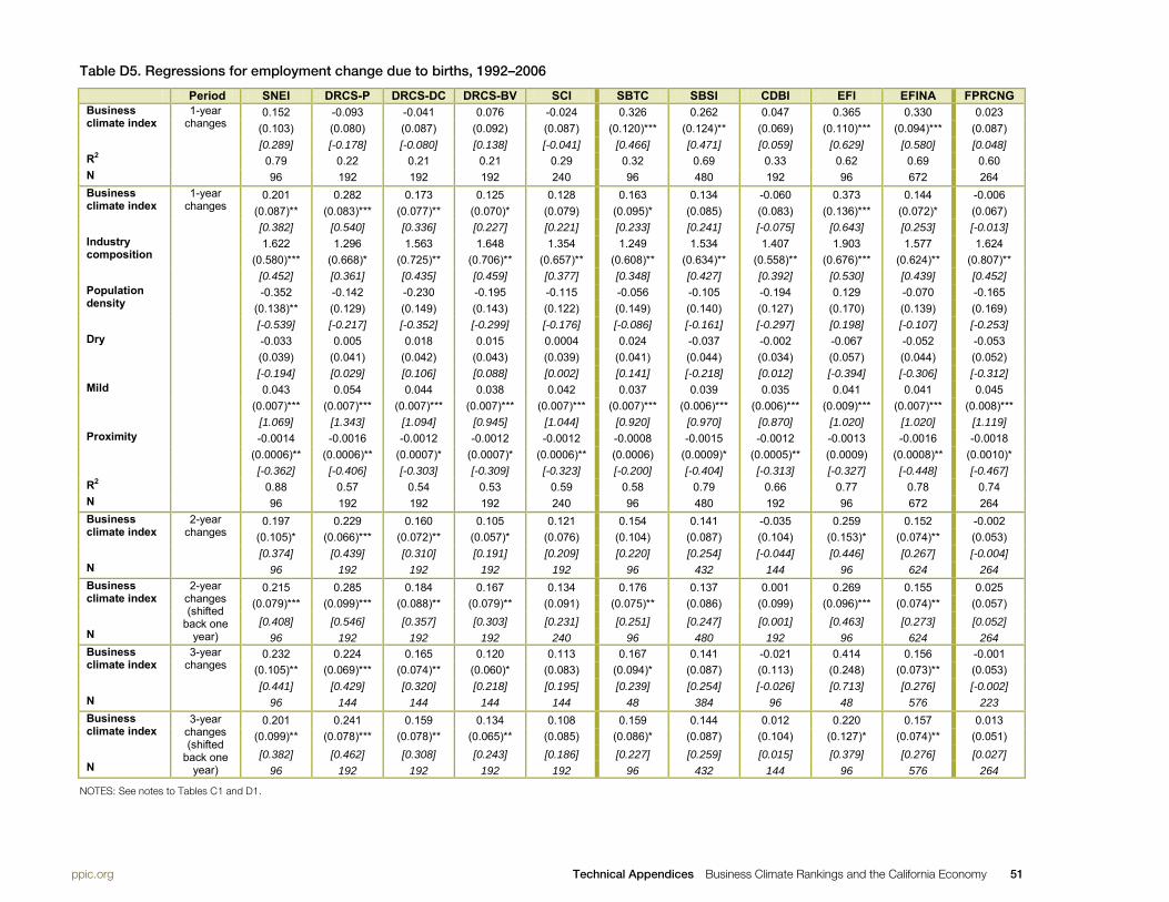
http://www.ppic.org/main/home.asp Technical Appendices Business Climate Rankings and the California Economy 51
Table D5. Regressions for employment change due to births, 1992–2006
Period SNEI DRCS-P DRCS-DC DRCS-BV SCI SBTC SBSI CDBI EFI EFINA FPRCNG Business climate index
1-year changes
0.152 -0.093 -0.041 0.076 -0.024 0.326 0.262 0.047 0.365 0.330 0.023 (0.103) (0.080) (0.087) (0.092) (0.087) (0.120)*** (0.124)** (0.069) (0.110)*** (0.094)*** (0.087) [0.289] [-0.178] [-0.080] [0.138] [-0.041] [0.466] [0.471] [0.059] [0.629] [0.580] [0.048]
R2 0.79 0.22 0.21 0.21 0.29 0.32 0.69 0.33 0.62 0.69 0.60 N 96 192 192 192 240 96 480 192 96 672 264 Business climate index
1-year changes
0.201 0.282 0.173 0.125 0.128 0.163 0.134 -0.060 0.373 0.144 -0.006 (0.087)** (0.083)*** (0.077)** (0.070)* (0.079) (0.095)* (0.085) (0.083) (0.136)*** (0.072)* (0.067) [0.382] [0.540] [0.336] [0.227] [0.221] [0.233] [0.241] [-0.075] [0.643] [0.253] [-0.013]
Industry composition
1.622 1.296 1.563 1.648 1.354 1.249 1.534 1.407 1.903 1.577 1.624 (0.580)*** (0.668)* (0.725)** (0.706)** (0.657)** (0.608)** (0.634)** (0.558)** (0.676)*** (0.624)** (0.807)**
[0.452] [0.361] [0.435] [0.459] [0.377] [0.348] [0.427] [0.392] [0.530] [0.439] [0.452] Population density
-0.352 -0.142 -0.230 -0.195 -0.115 -0.056 -0.105 -0.194 0.129 -0.070 -0.165 (0.138)** (0.129) (0.149) (0.143) (0.122) (0.149) (0.140) (0.127) (0.170) (0.139) (0.169)
[-0.539] [-0.217] [-0.352] [-0.299] [-0.176] [-0.086] [-0.161] [-0.297] [0.198] [-0.107] [-0.253] Dry -0.033 0.005 0.018 0.015 0.0004 0.024 -0.037 -0.002 -0.067 -0.052 -0.053 (0.039) (0.041) (0.042) (0.043) (0.039) (0.041) (0.044) (0.034) (0.057) (0.044) (0.052) [-0.194] [0.029] [0.106] [0.088] [0.002] [0.141] [-0.218] [0.012] [-0.394] [-0.306] [-0.312] Mild 0.043 0.054 0.044 0.038 0.042 0.037 0.039 0.035 0.041 0.041 0.045 (0.007)*** (0.007)*** (0.007)*** (0.007)*** (0.007)*** (0.007)*** (0.006)*** (0.006)*** (0.009)*** (0.007)*** (0.008)*** [1.069] [1.343] [1.094] [0.945] [1.044] [0.920] [0.970] [0.870] [1.020] [1.020] [1.119] Proximity -0.0014 -0.0016 -0.0012 -0.0012 -0.0012 -0.0008 -0.0015 -0.0012 -0.0013 -0.0016 -0.0018 (0.0006)** (0.0006)** (0.0007)* (0.0007)* (0.0006)** (0.0006) (0.0009)* (0.0005)** (0.0009) (0.0008)** (0.0010)* [-0.362] [-0.406] [-0.303] [-0.309] [-0.323] [-0.200] [-0.404] [-0.313] [-0.327] [-0.448] [-0.467] R2 0.88 0.57 0.54 0.53 0.59 0.58 0.79 0.66 0.77 0.78 0.74 N 96 192 192 192 240 96 480 192 96 672 264 Business climate index
2-year changes
0.197 0.229 0.160 0.105 0.121 0.154 0.141 -0.035 0.259 0.152 -0.002 (0.105)* (0.066)*** (0.072)** (0.057)* (0.076) (0.104) (0.087) (0.104) (0.153)* (0.074)** (0.053) [0.374] [0.439] [0.310] [0.191] [0.209] [0.220] [0.254] [-0.044] [0.446] [0.267] [-0.004]
N 96 192 192 192 192 96 432 144 96 624 264 Business climate index
2-year changes (shifted
back one year)
0.215 0.285 0.184 0.167 0.134 0.176 0.137 0.001 0.269 0.155 0.025 (0.079)*** (0.099)*** (0.088)** (0.079)** (0.091) (0.075)** (0.086) (0.099) (0.096)*** (0.074)** (0.057)
[0.408] [0.546] [0.357] [0.303] [0.231] [0.251] [0.247] [0.001] [0.463] [0.273] [0.052] N 96 192 192 192 240 96 480 192 96 624 264 Business climate index
3-year changes
0.232 0.224 0.165 0.120 0.113 0.167 0.141 -0.021 0.414 0.156 -0.001 (0.105)** (0.069)*** (0.074)** (0.060)* (0.083) (0.094)* (0.087) (0.113) (0.248) (0.073)** (0.053) [0.441] [0.429] [0.320] [0.218] [0.195] [0.239] [0.254] [-0.026] [0.713] [0.276] [-0.002]
N 96 144 144 144 144 48 384 96 48 576 223 Business climate index
3-year changes (shifted
back one year)
0.201 0.241 0.159 0.134 0.108 0.159 0.144 0.012 0.220 0.157 0.013 (0.099)** (0.078)*** (0.078)** (0.065)** (0.085) (0.086)* (0.087) (0.104) (0.127)* (0.074)** (0.051) [0.382] [0.462] [0.308] [0.243] [0.186] [0.227] [0.259] [0.015] [0.379] [0.276] [0.027]
N 96 192 192 192 192 96 432 144 96 576 264
NOTES: See notes to Tables C1 and D1.
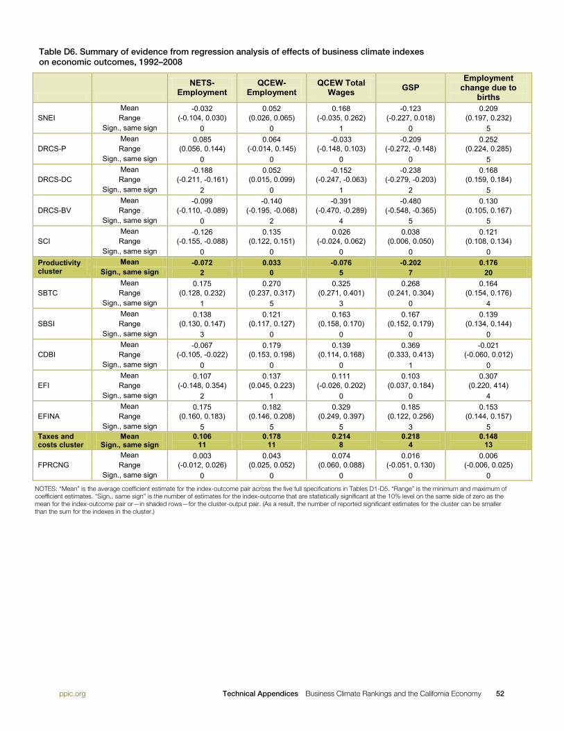
http://www.ppic.org/main/home.asp Technical Appendices Business Climate Rankings and the California Economy 52
Table D6. Summary of evidence from regression analysis of effects of business climate indexes on economic outcomes, 1992–2008
NETS-Employment
QCEW-Employment
QCEW Total Wages GSP
Employment change due to
births
SNEI Mean -0.032 0.052 0.168 -0.123 0.209 Range (-0.104, 0.030) (0.026, 0.065) (-0.035, 0.262) (-0.227, 0.018) (0.197, 0.232)
Sign., same sign 0 0 1 0 5
DRCS-P Mean 0.085 0.064 -0.033 -0.209 0.252 Range (0.056, 0.144) (-0.014, 0.145) (-0.148, 0.103) (-0.272, -0.148) (0.224, 0.285)
Sign., same sign 0 0 0 0 5
DRCS-DC Mean -0.188 0.052 -0.152 -0.238 0.168 Range (-0.211, -0.161) (0.015, 0.099) (-0.247, -0.063) (-0.279, -0.203) (0.159, 0.184)
Sign., same sign 2 0 1 2 5
DRCS-BV Mean -0.099 -0.140 -0.391 -0.480 0.130 Range (-0.110, -0.089) (-0.195, -0.068) (-0.470, -0.289) (-0.548, -0.365) (0.105, 0.167)
Sign., same sign 0 2 4 5 5
SCI Mean -0.126 0.135 0.026 0.038 0.121 Range (-0.155, -0.088) (0.122, 0.151) (-0.024, 0.062) (0.006, 0.050) (0.108, 0.134)
Sign., same sign 0 0 0 0 0 Productivity cluster
Mean -0.072 0.033 -0.076 -0.202 0.176 Sign., same sign 2 0 5 7 20
SBTC Mean 0.175 0.270 0.325 0.268 0.164 Range (0.128, 0.232) (0.237, 0.317) (0.271, 0.401) (0.241, 0.304) (0.154, 0.176)
Sign., same sign 1 5 3 0 4
SBSI Mean 0.138 0.121 0.163 0.167 0.139 Range (0.130, 0.147) (0.117, 0.127) (0.158, 0.170) (0.152, 0.179) (0.134, 0.144)
Sign., same sign 3 0 0 0 0
CDBI Mean -0.067 0.179 0.139 0.369 -0.021 Range (-0.105, -0.022) (0.153, 0.198) (0.114, 0.168) (0.333, 0.413) (-0.060, 0.012)
Sign., same sign 0 0 0 1 0
EFI Mean 0.107 0.137 0.111 0.103 0.307 Range (-0.148, 0.354) (0.045, 0.223) (-0.026, 0.202) (0.037, 0.184) (0.220, 414)
Sign., same sign 2 1 0 0 4
EFINA Mean 0.175 0.182 0.329 0.185 0.153 Range (0.160, 0.183) (0.146, 0.208) (0.249, 0.397) (0.122, 0.256) (0.144, 0.157)
Sign., same sign 5 5 5 3 5 Taxes and costs cluster
Mean Sign., same sign
0.106 11
0.178 11
0.214 8
0.218 4
0.148 13
FPRCNG Mean 0.003 0.043 0.074 0.016 0.006 Range (-0.012, 0.026) (0.025, 0.052) (0.060, 0.088) (-0.051, 0.130) (-0.006, 0.025)
Sign., same sign 0 0 0 0 0
NOTES: “Mean” is the average coefficient estimate for the index-outcome pair across the five full specifications in Tables D1-D5. “Range” is the minimum and maximum of coefficient estimates. “Sign., same sign” is the number of estimates for the index-outcome that are statistically significant at the 10% level on the same side of zero as the mean for the index-outcome pair or—in shaded rows—for the cluster-output pair. (As a result, the number of reported significant estimates for the cluster can be smaller than the sum for the indexes in the cluster.)

http://www.ppic.org/main/home.asp Technical Appendices Business Climate Rankings and the California Economy 53
Table D7. Regressions for QCEW Employment and Wages in Manufacturing and Footloose Industries, 1992-2008
Industry SNEI DRCS-P DRCS-DC DRCS-BV SCI SBTC SBSI CDBI EFI EFINA FPRCNG A. Employment Total private 0.055 -0.049 -0.001 -0.254 0.106 0.262 0.129 0.223 0.168 0.215 0.019
(0.087) (0.103) (0.092) (0.106)** (0.106) (0.101)** (0.081) (0.137) (0.172) (0.076)*** (0.060)
[0.105] [-0.092] [-0.002] [-0.457] [0.185] [0.387] [0.228] [0.277] [0.289] [0.378] [0.04]
Manufacturing -0.292 -0.271 -0.099 -0.563 0.053 0.526 0.328 0.858 -0.086 0.278 0.031
(0.215) (0.269) (0.243) (0.182)*** (0.225) (0.213)** (0.145)** (0.259)*** (0.356) (0.150)* (0.114)
[-0.558] [-0.509] [-0.184] [-1.014] [0.092] [0.778] [0.579] [1.066] [-0.148] [0.489] [0.065]
Footloose 0.329 -0.047 0.002 -0.271 0.197 0.235 0.195 0.381 0.047 0.251 0.196 industries (0.190)* (0.196) (0.152) (0.161)* (0.142) (0.148) (0.118) (0.144)** (0.460) (0.116)** (0.152)
[0.629] [-0.088] [0.004] [-0.488] [0.343] [0.348] [0.344] [0.473] [0.081] [0.441] [0.409]
B. Wages
Total private 0.326 -0.200 -0.248 -0.555 -0.077 0.301 0.187 0.188 0.210 0.397 0.075
(0.182)* (0.187) (0.148)* (0.161)*** (0.153) (0.207) (0.128) (0.284) (0.271) (0.088)*** (0.108)
[0.623] [-0.376] [-0.462] [-0.999] [-0.134] [0.445] [0.33] [0.233] [0.362] [0.698] [0.156] Manufacturing 0.187 -0.217 -0.179 -0.650 0.141 0.688 0.336 0.643 -0.784 0.373 0.231
(0.399) (0.356) (0.267) (0.218)*** (0.263) (0.257)** (0.171)* (0.353)* (0.697) (0.161)** (0.182)
[0.357] [-0.408] [-0.334] [-1.17] [0.246] [1.017] [0.593] [0.799] [-1.351] [0.656] [0.481] Footloose 0.805 -0.175 -0.227 -0.388 0.058 0.148 0.190 0.104 0.571 0.474 0.129 industries (0.252)*** (0.239) (0.235) (0.297) (0.251) (0.245) (0.175) (0.243) (0.478) (0.148)*** (0.174)
[1.539] [-0.329] [-0.423] [-0.699] [0.101] [0.219] [0.335] [0.129] [0.984] [0.834] [0.269] N 144 288 288 288 336 192 576 288 96 672 309
NOTES: See notes to Tables C1 and D1. Employment and wages data cover private sector only. The dependent variable is 1-year changes of the variable in the first column, and all controls are included, so the specifications correspond to the second ones Tables D1–D5. Manufacturing employment corresponds to NAICS codes 31–33, and footloose industries are information (51), finance and insurance (52), and professional and technical services (54).

http://www.ppic.org/main/home.asp Technical Appendices Business Climate Rankings and the California Economy 54
Figure D1. QCEW employment growth vs. index averages, scatterplots of data and regression residuals
AL
AZ
AR CA
CO
CT
DE
FLGA
ID
ILIN
IAKSKY
LA MEMD
MA
MI
MN
MS MO
MT
NE
NV
NH
NJ
NM
NY
NC
ND
OH
OK
OR
PARI
SC
SD
TN
TX
UT
VT
VAWA
WV
WI
WY
Slope (Std. Err.)=0.031 (0.145)
0
1
2
3
4
QCEW
em
ploy
men
t cha
nge
1992
-200
8 an
nual
ized
-2 -1 0 1 2
Average business climate index for productivity cluster
Productivity cluster
AL
AZ
ARCA
CO
CT
DE
FLGA
ID
IL IN
IAKSKY
LAMEMD
MA
MI
MN
MSMO
MT
NE
NV
NH
NJ
NM
NY
NC
ND
OH
OK
OR
PARI
SC
SD
TN
TX
UT
VT
VAWA
WV
WI
WY
Slope (Std. Err.) = 0.559 (0.126)0
1
2
3
4
QCE
W e
mpl
oym
ent c
hang
e 19
92-2
008
annu
alize
d
-2 -1 0 1 2
Average business climate index for taxes-and-costs cluster
Taxes-and-costs cluster

http://www.ppic.org/main/home.asp Technical Appendices Business Climate Rankings and the California Economy 55
Figure D2. Contributions of business climate index and control variables to employment growth (QCEW)
NOTE: Presents product of coefficients from Table D2 and states’ values for business climate index and control variables relative to mean. Units are percentage points of annual employment growth. Averaged over values from SBTC, EFI, and EFINA models. The California datapoint corresponds to the second set of bars in Figure 2 in the main text.
CTME
MANH
NJ
NY
PA
RI
VT
IL
IN
IA
KS
MIMN
MONE
ND
OH
SD
WI AL
AR
DE
FL
GA
KY
LA
MD
MSNC
OK
SC
TN
TX
VA
WV
AZ
CA
CO
ID
MT
NV
NM
OR
UT
WA
WY
-1
-.5
0
.5
1
1.5
2
Cont
ribut
ion
of c
ontro
l var
iables
-.5 0 .5 1
Contribution of business climate
Northeast Midwest South West
All regions

http://www.ppic.org/main/home.asp Technical Appendices Business Climate Rankings and the California Economy 56
Table D8. Single sub-index regressions
NETS Employment
QCEW Employment
QCEW Total Wages GSP
Employment change due
to births SBTC corporate 0.222 0.241 0.463 0.490 0.120 income tax sub-index (0.090)** (0.073)*** (0.153)*** (0.124)*** (0.079)
[0.241] [0.251] [0.481] [0.509] [0.130] SBTC individual 0.143 0.187 0.232 0.216 0.129 income tax sub-index (0.124) (0.088)** (0.157) (0.183) (0.082)
[0.185] [0.232] [0.288] [0.268] [0.167] SBTC sales tax sub-index 0.140 -0.026 -0.187 -0.383 0.052
(0.104) (0.098) (0.091)** (0.151)** (0.064)
[0.125] [-0.023] [-0.167] [-0.341] [0.046] SBTC property tax -0.223 0.102 -0.028 0.231 -0.001 sub-index (0.136) (0.096) (0.165) (0.189) (0.080)
[-0.388] [0.179] [-0.049] [0.406] [-0.002] SBTC Unemployment -0.025 0.038 0.039 0.072 -0.051 Insurance tax sub-index (0.122) (0.068) (0.123) (0.144) (0.085)
[-0.043] [0.068] [0.069] [0.128] [-0.088] N 96 192 192 192 96
EFINA size of 0.226 0.251 0.399 0.194 0.169 government sub-index (0.080)*** (0.066)*** (0.074)*** (0.110)* (0.067)**
[0.398] [0.442] [0.702] [0.342] [0.298] EFINA labor market 0.087 0.153 0.329 0.280 0.102 freedom sub-index (0.110) (0.104) (0.126)** (0.144)* (0.092)
[0.126] [0.221] [0.476] [0.405] [0.147] EFINA takings and 0.107 0.127 0.227 0.117 0.097 discriminatory taxation (0.085) (0.067)* (0.087)** (0.109) (0.069) sub-index [0.185] [0.22] [0.392] [0.202] [0.168] N 672 672 672 432 672
EFI fiscal sub-index 0.068 0.126 0.099 -0.068 0.103
(0.142) (0.161) (0.249) (0.312) (0.114)
[0.117] [0.216] [0.17] [-0.117] [0.177] EFI regulatory sub-index 0.087 -0.042 -0.010 0.011 0.133
(0.170) (0.122) (0.196) (0.305) (0.111)
[0.137] [-0.066] [-0.016] [0.017] [0.209] EFI welfare spending 0.453 0.290 0.401 0.428 0.364 sub-index (0.162)*** (0.124)** (0.197)** (0.277) (0.134)***
[0.669] [0.429] [0.593] [0.632] [0.538] EFI government size 0.175 0.176 0.402 0.202 0.210 sub-index (0.157) (0.094)* (0.173)** (0.172) (0.086)**
[0.29] [0.292] [0.667] [0.335] [0.348] EFI judicial sub-index 0.106 -0.084 -0.094 -0.091 0.117
(0.151) (0.110) (0.221) (0.248) (0.088)
[0.208] [-0.165] [-0.185] [-0.179] [0.230] N 96 96 96 96 96
NOTES: Every cell reports a different regression. The dependent variable is 1-year changes of the variable in the first row, and all controls are included, so the specifications correspond to the second ones in Tables D1-D5.

http://www.ppic.org/main/home.asp Technical Appendices Business Climate Rankings and the California Economy 57
Table D9. Regressions including all sub-indexes within an index
NETS Employment
QCEW Employment
QCEW Total Wages GSP
Employment change due
to births SBTC corporate income 0.211 0.212 0.467 0.513 0.074 tax sub-index (0.137) (0.131) (0.205)** (0.226)** (0.100)
[0.229] [0.220] [0.485] [0.533] [0.080] SBTC individual income 0.048 0.081 -0.028 -0.089 0.105 tax sub-index (0.165) (0.135) (0.198) (0.253) (0.099)
[0.062] [0.101] [-0.035] [-0.111] [0.136] SBTC sales tax sub-index 0.214 0.014 -0.102 -0.336 0.088
(0.108)* (0.082) (0.099) (0.151)** (0.067)
[0.191] [0.012] [-0.091] [-0.299] [0.078] SBTC property tax sub-index -0.209 0.133 0.045 0.343 0.010
(0.130) (0.085) (0.144) (0.188)* (0.078)
[-0.364] [0.234] [0.079] [0.604] [0.017] SBTC Unemployment -0.029 0.053 0.071 0.134 -0.054 Insurance tax sub-index (0.116) (0.066) (0.124) (0.146) (0.084)
[-0.050] [0.094] [0.127] [0.239] [-0.094] N 96 192 192 192 96 R2 0.55 0.50 0.49 0.44 0.59
EFINA size of 0.359 0.356 0.473 0.147 0.218 government sub-index (0.128)*** (0.122)*** (0.145)*** (0.151) (0.104)**
[0.632] [0.627] [0.833] [0.259] [0.384] EFINA labor market -0.066 0.002 0.117 0.222 -0.001 freedom sub-index (0.119) (0.116) (0.138) (0.163) (0.099)
[-0.095] [0.003] [0.169] [0.321] [-0.001] EFINA takings and -0.129 -0.128 -0.150 -0.061 -0.059 discriminatory taxation (0.134) (0.116) (0.142) (0.133) (0.099) sub-index [-0.223] [-0.221] [-0.259] [-0.105] [-0.102] N 672 672 672 432 672 R2 0.77 0.68 0.61 0.29 0.78
EFI fiscal sub-index -0.134 0.073 -0.024 -0.243 -0.077
(0.132) (0.172) (0.249) (0.276) (0.096)
[-0.230] [0.125] [-0.041] [-0.417] [-0.132] EFI regulatory sub-index -0.021 -0.157 -0.148 -0.073 0.041
(0.170) (0.118) (0.195) (0.288) (0.096)
[-0.033] [-0.247] [-0.233] [-0.115] [0.064] EFI welfare spending 0.461 0.308 0.367 0.534 0.299 sub-index (0.168)*** (0.146)** (0.231) (0.275)* (0.138)**
[0.681] [0.455] [0.542] [0.789] [0.442] EFI government size 0.095 0.101 0.326 0.095 0.159 sub-index (0.149) (0.102) (0.201) (0.186) (0.084)*
[0.158] [0.168] [0.541] [0.158] [0.264] EFI judicial sub-index 0.078 -0.105 -0.083 -0.115 0.108
(0.142) (0.112) (0.225) (0.258) (0.075)
[0.153] [-0.206] [-0.163] [-0.226] [0.212] N 96 96 96 96 96 R2 0.77 0.43 0.52 0.38 0.78
NOTES: See notes to Table D8. In this table, all sub-indexes within an index are included simultaneously.

http://www.ppic.org/main/home.asp Technical Appendices Business Climate Rankings and the California Economy 58
Table D10. Summary of evidence from regression analysis of effects of business climate sub-indexes on economic outcomes, 1992–2008
Sub-index
NETS-Employment
QCEW-Employment
QCEW Total Wages GSP
Employment change due to
births
SBTC-CTI Mean 0.174 0.208 0.460 0.522 0.058 Range (0.111, 0.234) (0.199, 0.222) (0.443, 0.476) (0.494, 0.549) (0.046, 0.074)
Sign., same sign 1 1 5 5 0
SBTC-IITI Mean 0.048 0.116 0.027 -0.088 0.121 Range (0.031, 0.065) (0.079, 0.175) (-0.028, 0.096) (-0.115, -0.064) (0.105, 0.135)
Sign., same sign 0 0 0 0 1
SBTC-STI Mean 0.091 0.041 -0.053 -0.214 0.077 Range (0.020, 0.214) (0.012, 0.087) (-0.102, 0.016) (-0.336, -0.114) (0.057, 0.104)
Sign., same sign 1 0 0 2 1
SBTC-PTI Mean -0.131 0.124 0.010 0.157 0.032 Range (-0.209, -0.095) (0.104, 0.140) (-0.013, 0.045) (0.035, 0.343) (0.010, 0.068)
Sign., same sign 0 0 0 1 0
SBTC-UITI
Mean -0.059 -0.019 -0.014 0.082 -0.051
Range (-0.153, -0.007) (-0.073, 0.053) (-0.099, 0.071) (0.020,0.134) (-0.069, -0.036)
Sign., same sign 0 0 0 0 0
EFINA-SG Mean 0.331 0.326 0.449 0.129 0.229 Range (0.306, 0.359) (0.270, 0.379) (0.371, 0.523) (0.068, 0.185) (0.218, 0.235)
Sign., same sign 5 5 5 0 5
EFINA-LMF Mean -0.031 -0.001 0.108 0.207 0.001 Range (-0.066, -0.013) (-0.009, 0.003) (0.097, 0.117) (0.198, 0.222) (-0.005, 0.008)
Sign., same sign 0 0 0 0 0
EFINA-TDT Mean -0.110 -0.120 -0.151 -0.046 -0.062
Range (-0.129, -0.088) (-0.138, -0.104) (-0.155, -0.143) (-0.067, -0.023) (-0.073, -0.056) Sign., same sign 0 0 0 0 0
EFI-F Mean -0.051 0.031 -0.042 -0.156 -0.047 Range (-0.134, 0.088) (-0.052, 0.102) (-0.129, 0.035) (-0.260, 0.014) (-0.101, 0.008)
Sign., same sign 0 0 0 0 0
EFI-R Mean -0.097 -0.136 -0.165 -0.093 -0.046 Range (-0.221, -0.021) (-0.211, -0.047) (-0.218, -0.121) (-0.210, 0.010) (-0.119, 0.041)
Sign., same sign 0 1 0 0 0
EFI-WS Mean 0.156 0.246 0.325 0.419 0.293 Range (-0.037, 0.461) (0.186, 0.308) (0.263, 0.375) (0.212, 0.534) (0.232, 0.403)
Sign., same sign 1 3 3 4 4
EFI-GS Mean 0.136 0.098 0.172 0.035 0.156 Range (0.095, 0.167) (0.015, 0.168) (-0.044, 0.350) (-0.086, 0.104) (0.123, 0.242)
Sign., same sign 1 0 1 0 3
EFI-J Mean 0.165 -0.112 -0.196 -0.261 0.167 Range (0.073, 0.319) (-0.137, -0.076) (-0.283, -0.083) (-0.373, -0.115) (0.108, 0.250)
Sign., same sign 0 0 3 2 4
NOTES: “Mean” is the average coefficient estimate for the sub-index-outcome pairs across the same five full specifications in Tables D1-D5. “Range” is the minimum and maximum of coefficient estimates. “Sign., same sign” is the number of estimates for the sub-index-outcome that are statistically significant at the 10% level on the same side of zero as the mean for the sub-index-outcome pair.

http://www.ppic.org/main/home.asp Technical Appendices Business Climate Rankings and the California Economy 59
Table D11. Qualitative summary of evidence from regression analysis of effects of business climate sub-indexes on economic outcomes, 1992–2008
NOTES: See Tables D9 and D10 for detailed results. The characterization of the detailed results summarized in this table is based on the sign and statistical significance of the results across numerous specifications. The NETS data go only through 2006. The second column reports, as needed, the main content of the sub-index; for additional details see Table A6a and Table A5.
Content of sub-index
NETS Employment
QCEW Employment
QCEW Total Wages GSP
SBTC corporate income tax index
Structure, base, and rate of corporate tax
No effect or positive
No effect or positive Clear positive Clear positive
SBTC individual income tax index
Structure, base, and rate of individual
income tax No effect No effect No effect No effect
SBTC sales tax index Structure, base, and rate of sales tax
No effect or positive No effect No effect No effect or
negative
SBTC property tax index Structure, base, and rate of property tax No effect No effect No effect No effect or
positive SBTC unemployment insurance tax index
Structure and rate of UI tax No effect No effect No effect No effect
EFINA size of government index
Mainly welfare and transfer payments Clear positive Clear positive Clear positive No effect
EFINA labor market freedom index
Mainly costs of doing business (excl. taxes) No effect No effect No effect No effect
EFINA takings and discriminatory taxation index
Tax rates and tax burden No effect No effect No effect No effect
EFI fiscal index Mainly tax rates and tax burden No effect No effect No effect No effect
EFI regulatory index Regulations and regulatory structure No effect No effect or
negative No effect No effect
EFI welfare spending index Mainly welfare and transfer payments
No effect or positive Positive Positive Clear positive
EFI government size index Overall government expenditures and
employment
No effect or positive No effect No effect or
positive No effect
EFI judicial index Litigation rules and judiciary characterstics No effect No effect Negative No effect or
negative

http://www.ppic.org/main/home.asp Technical Appendices Business Climate Rankings and the California Economy 60
References
Albouy, David. 2009. “What Are Cities Worth? Land Rents, Local Productivity, and the Capitalization of Amenity Values.” NBER Working Paper No. 14981.
Anderson Economic Group. 2006. “Benchmarking for Success: A Comparison of State Business Taxes.” Report commissioned by the Michigan House of Representatives. Available at www.andersoneconomicgroup.com/LinkClick.aspx?link=upload%2fDoc1950.pdf&tabid=125&mid=411.
Atkinson, Robert D., and Scott M. Andes. 2008. “The 2008 State New Economy Index: Benchmarking Economic Transformation in the States.” Washington DC: Information Technology and Innovation Foundation.
Bartik, Timothy J. 1985. “Business Location Decisions in the United States: Estimates of the Effects of Unionization, Taxes, and Other Characteristics of States.” Journal of Business & Economic Statistics 3: 14–22.
Bartik, Timothy J. 1991. Who Benefits from State and Local Economic Development Policies? Kalamazoo, MI: W. E. Upjohn Institute for Employment Research.
Bartik, Timothy J. 1994. “Jobs, Productivity, and Local Economic Development: What Implications Does Economic Research Have for the Role of Government?” National Tax Journal 47: 847–61.
Beacon Hill Institute.2008. “Eighth Annual State Competitiveness Report.” Available at www.beaconhill.org/Compete08/BHIState08-FINAL.pdf.
Besley, Timothy, and Anne Case. 1995. “Does Electoral Accountability Affect Economic Policy Choices? Evidence from Gubernatorial Term Limits.” Quarterly Journal of Economics 110: 769–98.
Bittlingmayer, George, Liesl Eathington, Arthur P. Hall, and Peter F. Orazem. 2005. “Business Climate Indexes: Which Work, Which Don’t, and What Can They Say about the Kansas Economy?” Research report prepared for Kansas, Inc. Available at www.kansasinc.org/pubs/working/Business%20Climate%20Indexes.pdf.
Blank, Rebecca M. 2002. “Evaluating Welfare Reform in the United States.” Journal of Economic Literature 40: 1105–66.
Brueckner, Jan. 2001. “Strategic Interaction Among Governments: An Overview of Empirical Studies.” International Regional Science Review 26: 175–88.
Buss, Terry F. 2001. “The Effect of State Tax Incentives on Economic Growth and Firm Location Decisions: An Overview of the Literature.” Economic Development Quarterly 15: 90–105.
Carlton, Dennis W. 1983. “The Location and Employment Choices of New Firms: An Econometric Model with Discrete and Continuous Endogenous Variables.” Review of Economics and Statistics 65: 440–49.
Crain, W. Mark, and Katherine J. Lee. 1999. “Economic Growth Regressions for the American States: A Sensitivity Analysis.” Economic Inquiry 37: 242–57.
Dardia, Michael, and Sherman Luk. 1999. “Rethinking the California Business Climate.” San Francisco: Public Policy Institute of California.
Davis, Steven, John Haltiwanger, and Scott Schuh. 1996. Job Creation and Destruction. Cambridge, MA: MIT Press.
Dubay, Curtis, and Chris Atkins. 2006. “2007 State Business Tax Climate Index,” Background Paper No. 52. Washington DC: Tax Foundation.
Elmendorf, Doug, and Jason Furman. 2008. “If, When, How: A Primer on Fiscal Stimulus.” Hamilton Project Strategy Paper. Washington DC: Brookings Institution.
Erickson, Rodney A. 1987. “Business Climate Studies: A Critical Evaluation.” Economic Development Quarterly 1: 62–71.
Fisher, Peter. 2005. Grading Places, Washington DC: Economic Policy Institute.
Gabriel, Stuart A., and Stuart S. Rosenthal. 2004. “Quality of the Business Environment versus Quality of Life: Do Firms and Households Like the Same Cities?” Review of Economics and Statistics 86: 438–44.
Garrett, Thomas, and Russell Rhine. 2010. “Economic Freedom and Employment Growth in U.S. States.” Federal Reserve Bank of St. Louis Working Paper 2010-006A.
Glaeser, Edward, et al. 1992. “Growth in Cities.” Journal of Political Economy 100: 1126–52.

http://www.ppic.org/main/home.asp Technical Appendices Business Climate Rankings and the California Economy 61
Glaeser, Edward L., and Matthew E. Kahn. 2004. “Sprawl and Urban Growth.” In Handbook of Regional and Urban Economics, vol. 4, ed. J. V. Henderson and J. F. Thisse (Amsterdam: Elsevier B.V.), 2482–2527.
Glaeser, Edward, Jed Kolko, and Albert Saiz. 2001. “Consumer City.” Journal of Economic Geography 1: 27–50.
Greenstone, Michael, Richard Hornbeck, and Enrico Moretti. 2007. “Identifying Agglomeration Spillovers: Evidence from Million Dollar Plants.” MIT Department of Economics Working Paper No. 07-31.
Haltiwanger, John, Ron S. Jarmin, and Javier Miranda. 2009. “Who Creates Jobs? Small vs. Large vs. Young.” Unpublished paper, University of Maryland.
Helms, L. Jay. 1985. “The Effect of State and Local Taxes on Economic Growth: A Time Series—Cross Section Approach.” Review of Economics and Statistics 67: 574–82.
Henderson, Vernon, Ari Kuncoro, and Matt Turner. 1995. “Industrial Development in Cities.” Journal of Political Economy 103: 1067–90.
Holmes, Thomas. 1998. “The Effect of State Policies on the Location of Manufacturing: Evidence from State Borders.” Journal of Political Economy 106: 667–705.
Kolko, Jed, and David Neumark. 2007. Business Location Decisions and Employment Dynamics in California. San Francisco: Public Policy Institute of California.
Kolko, Jed, and Davin Reed. 2008. “The California Economy: Employment in 2007.” Just the Facts. San Francisco: Public Policy Institute of California.
Laffer, Arthur, and Stephen Moore. 2007. Rich States Poor States: ALEC-Laffer State Economic Competitiveness Index. Washington DC: American Legislative Exchange Council.
Mendelsohn, Robert, William D. Nordhaus, and Daigee Shaw. 1994. “The Impact of Global Warming on Agriculture: A Ricardian Analysis.” American Economic Review 84: 753–71.
Mulligan, Casey, and Andrei Shleifer. 2005. “The Extent of the Market and the Supply of Regulation.” Quarterly Journal of Economics 120: 1445–73.
Neiman, Max, Gregory Andranovich, and Kenneth Fernandez. 2000. Local Economic Development in Southern California’s Suburbs: 1990–1997. San Francisco: Public Policy Institute of California.
Neumark, David, Brandon Wall, and Junfu Zhang. Forthcoming. “Do Small Businesses Create More Jobs? New Evidence for the United States from the National Establishment Time Series.” Review of Economics and Statistics.
Neumark, David, Junfu Zhang, and Brandon Wall. 2005. “Are Businesses Fleeing the State? Interstate Business Relocation and Employment Change in California.” California Economic Policy 1, Public Policy Institute of California.
Neumark, David, Junfu Zhang, and Brandon Wall. 2006. “Where the Jobs Are: Business Dynamics and Employment Growth.” Academy of Management Perspectives 20: 79–94.
Neumark, David, Junfu Zhang, and Brandon Wall. 2007. “Employment Dynamics and Business Relocation: New Evidence from the National Establishment Time Series.” Research in Labor Economics 26: 39–84.
Papke, Leslie E. 1991. “Interstate Business Tax Differentials and New Firm Location.” Journal of Public Economics 45: 47–68.
Papke, Leslie E. 1997. “Subnational Taxation and Capital Mobility: Estimates of Tax-Price Elasticities.” National Tax Journal 40: 191–204.
Plaut, Thomas, and Joseph Pluta. 1983. “Business Climate, Taxes and Expenditures, and State Industrial Growth in the United States.” Southern Economic Journal 50: 99–119.
Rappaport, Jordan, and Jeffrey Sachs. 2003. “The United States as a Coastal Nation.” Journal of Economic Growth 8: 5–46.
Reed, W. Robert. 2009. “The Determinants of U.S. State Economic Growth: A Less Extreme Bounds Analysis.” Economic Inquiry 47: 685–700.
Roback, Jennifer. 1982. “Wages, Rents, and Quality of Life.” Journal of Political Economy 90: 1257–78.
Schumpeter, Joseph. 1942. Capitalism, Socialism, and Democracy. Repr., New York: Harper, 1975.
Shapiro, Jesse. 2006. “Smart Cities: Quality of Life, Productivity, and the Growth Effects of Human Capital.” Review of Economics and Statistics 88: 324–35.

http://www.ppic.org/main/home.asp Technical Appendices Business Climate Rankings and the California Economy 62
Slivinski, Stephen. 2006. “Fiscal Policy Report Card on America’s Governors: 2006.” Cato Institute Policy Analysis No. 581.
Skoro, Charles. 1988. “Rankings of State Business Climates: An Evaluation of Their Usefulness in Forecasting.” Economic Development Quarterly 2: 138–52.
Tannenwald, Robert. 1996. “State Business Tax Climate: How Should It Be Measured and How Important Is It?” New England Economic Review (January/February): 23–38.
Tannenwald, Robert. 1997. “State Regulatory Policy and Economic Development.” New England Economic Review (March/April): 83–99.
Varshney, Sanjay, and Dennis Tootelian. 2009. “Cost of State Regulations on California Small Business Study.” El Dorado Hills: Varshney and Associates.
Wasylenko, Michael. 1997. “Taxation and Economic Development: The State of the Economic Literature.” New England Economic Review (March/April): 37–52.
Wasylenko, Michael, and Therese McGuire. 1985. “Jobs and Taxes: The Effect of Business Climate on States’ Employment Growth Rates.” National Tax Journal 38: 497–511.

The Public Policy Institute of California is dedicated to informing and improving public policy in California through independent, objective, nonpartisan research on major economic, social, and political issues. The institute’s goal is to raise public awareness and to give elected representatives and other decisionmakers a more informed basis for developing policies and programs.
The institute’s research focuses on the underlying forces shaping California’s future, cutting across a wide range of public policy concerns, including economic development, education, environment and resources, governance, population, public finance, and social and health policy.
PPIC is a private operating foundation. It does not take or support positions on any ballot measures or on any local, state, or federal legislation, nor does it endorse, support, or oppose any political parties or candidates for public office. PPIC was established in 1994 with an endowment from William R. Hewlett.
Mark Baldassare is President and Chief Executive Officer of PPIC. John E. Bryson is Chair of the Board of Directors.
Short sections of text, not to exceed three paragraphs, may be quoted without written permission provided that full attribution is given to the source and the above copyright notice is included. Research publications reflect the views of the authors and do not necessarily reflect the views of the staff, officers, or Board of Directors of the Public Policy Institute of California.
© 2011 Public Policy Institute of California All rights reserved. San Francisco, CA
PUBLIC POLICY INSTITUTE OF CALIFORNIA 500 Washington Street, Suite 600 San Francisco, California 94111 phone: 415.291.4400 fax: 415.291.4401 www.ppic.org
PPIC SACRAMENTO CENTER Senator Office Building 1121 L Street, Suite 801 Sacramento, California 95814 phone: 916.440.1120 fax: 916.440.1121