BUSINESS UNDERSTANDING ­ Scania trucks

END TERM PROJECT ­ A.Y. 2016

Teacher: Students: Prof. Pasquale Rullo De Rosis Alessandro Francesco,180196

Lab Assistant: Pezzolla Daniele,139811

Prof. Ettore Ritacco Surace Luca,182458

Temesgen Zelalem,180416

Abstract

This document describes the analysis performed to understand and

manipulate a dataset in order to get the best classification possible. We

perform different analyzes in order to understand which algorithm best fits our

scenario and how to manipulate data to fit the model required by the algorithm

itself. The analysis was performed following the CRISP­DM methodology.

Business Understanding

The goal of this project is building a model based on an algorithm to predict

the component failure for a specific truck component. This model will be based

on the data gathered by the sensors and should signal all the deadline of the

components in order to optimize their replacement and troubleshooting.

Data understanding

Data description: The dataset is presented in 1 cvs file characterized by 60000 tuples: 59000

negative class and 1000 positive class. The positive class consists of

component failures for a specific component related to the APS system. The

negative class consists of trucks with failures for components not related to the

APS.

Attribute description: Each instances is described by 171 attributes, of which 7 are histogram

variables, all the attributes are expressed into numerical form. The attribute

names of the data have been anonymized for proprietary reasons, increasing

the data understanding difficulty. For this reason the semantic of each attribute

is not evaluable. They will be treated observing their distribution.

1

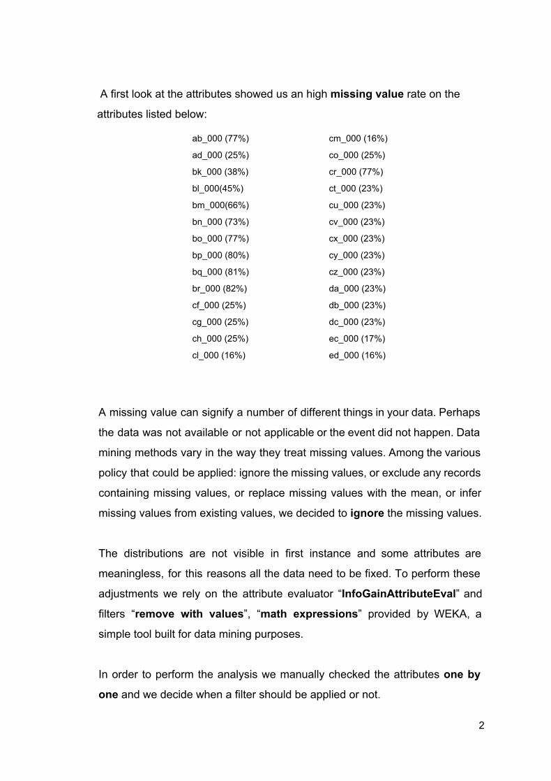
A first look at the attributes showed us an high missing value rate on the

attributes listed below:

ab_000 (77%)

ad_000 (25%)

bk_000 (38%)

bl_000(45%)

bm_000(66%)

bn_000 (73%)

bo_000 (77%)

bp_000 (80%)

bq_000 (81%)

br_000 (82%)

cf_000 (25%)

cg_000 (25%)

ch_000 (25%)

cl_000 (16%)

cm_000 (16%)

co_000 (25%)

cr_000 (77%)

ct_000 (23%)

cu_000 (23%)

cv_000 (23%)

cx_000 (23%)

cy_000 (23%)

cz_000 (23%)

da_000 (23%)

db_000 (23%)

dc_000 (23%)

ec_000 (17%)

ed_000 (16%)

A missing value can signify a number of different things in your data. Perhaps

the data was not available or not applicable or the event did not happen. Data

mining methods vary in the way they treat missing values. Among the various

policy that could be applied: ignore the missing values, or exclude any records

containing missing values, or replace missing values with the mean, or infer

missing values from existing values, we decided to ignore the missing values.

The distributions are not visible in first instance and some attributes are

meaningless, for this reasons all the data need to be fixed. To perform these

adjustments we rely on the attribute evaluator “InfoGainAttributeEval” and

filters “remove with values”, “math expressions” provided by WEKA, a

simple tool built for data mining purposes.

In order to perform the analysis we manually checked the attributes one by

one and we decide when a filter should be applied or not.

2

Figure 1 ­ How the attribute changes after the application of the logarithm

As we mentioned before, in the majority of the cases the distribution is not

highlighted. Applying the logarithm function is needed to better identify the

distribution. We chose this function for its great expansive capacity while it

maintains distribution property untouched. As we can show in the Figure 1

above.

For each attribute we use the filter “remove with values” that removes the

useless instances, after or before a threshold, in order to show better the

remaining distribution. The “pinnacle” at the beginning of an attribute graph

could be an huge amount of unnecessary data because in that area the

function distribution is constant. Thus it is impossible to get any predictive

properties. In this case we tried to use again the logarithm function but the

distribution did not change. Thus we use the filter “remove with values” as a

splitter, choosing the highest value of the range that contains the pinnacle as

split point. In the cases in which we observed that the majority of the instances

are contained by the pinnacle, then we preferred to remove the whole

attribute.

Since the red class (positive) counts less instances than the blue one

(negative), we used again the “Removes With Values” with different

parameters as an isolator tool. In this way, it has been possible to separate

the two graphs and make the best choice to ensure the analysis relevance.

3

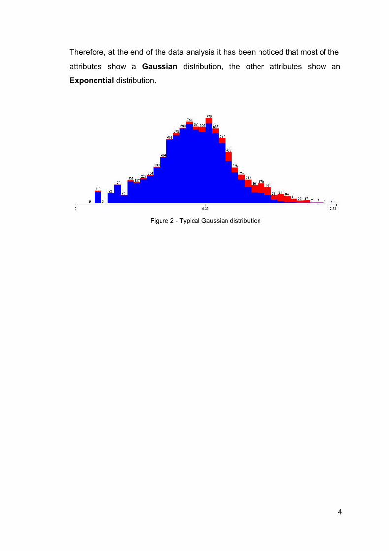
Therefore, at the end of the data analysis it has been noticed that most of the

attributes show a Gaussian distribution, the other attributes show an

Exponential distribution.

Figure 2 ­ Typical Gaussian distribution

4

Data Preparation:

Data Cleaning:

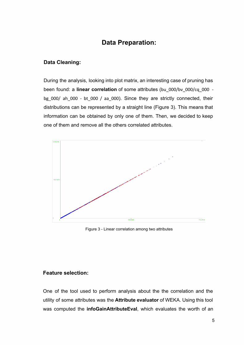
During the analysis, looking into plot matrix, an interesting case of pruning has

been found: a linear correlation of some attributes (bu_000/bv_000/cq_000 ­

bg_000/ ah_000 ­ bt_000 / aa_000). Since they are strictly connected, their

distributions can be represented by a straight line (Figure 3). This means that

information can be obtained by only one of them. Then, we decided to keep

one of them and remove all the others correlated attributes.

Figure 3 ­ Linear correlation among two attributes

Feature selection:

One of the tool used to perform analysis about the the correlation and the

utility of some attributes was theAttribute evaluator of WEKA. Using this tool

was computed the infoGainAttributeEval, which evaluates the worth of an

5

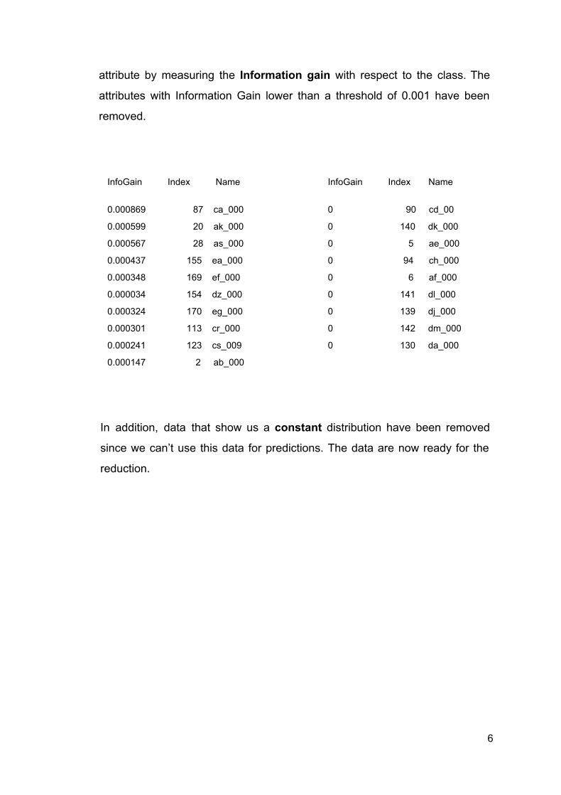
attribute by measuring the Information gain with respect to the class. The

attributes with Information Gain lower than a threshold of 0.001 have been

removed.

InfoGain Index Name InfoGain Index Name

0.000869 87 ca_000

0.000599 20 ak_000

0.000567 28 as_000

0.000437 155 ea_000

0.000348 169 ef_000

0.000034 154 dz_000

0.000324 170 eg_000

0.000301 113 cr_000

0.000241 123 cs_009

0.000147 2 ab_000

0 90 cd_00

0 140 dk_000

0 5 ae_000

0 94 ch_000

0 6 af_000

0 141 dl_000

0 139 dj_000

0 142 dm_000

0 130 da_000

In addition, data that show us a constant distribution have been removed

since we can’t use this data for predictions. The data are now ready for the

reduction.

6

Data Reduction

Sampling data: The training set was prepared splitting the original dataset in two different

sets, the training set and the test set. The first was used totrain the model and

the second to test what it learned. The test set was made using the wekafilter

“remove percentage”, extracting 30% of random tuples from the dataset and

checking with mysql that the training and the test set are disjoints.

We also tried the “Resample”(Unsupervised) filter to create our sets.

After that, we started to prepare the training set for the subsequent algorithms.

In order to create a subset of the original training data that maintains similar

statistical behaviour we applied a data preparation filter calledSampling. The

WEKA version of this procedure is called Resample. It has been applied to our

dataset, pruning the 25% of the original tuples, decreasing the total of

instances to 10499 and balancing the ratio between the two classes with

different uniform value ( 0.3 ­ 0.4 ­ 0.5).

7

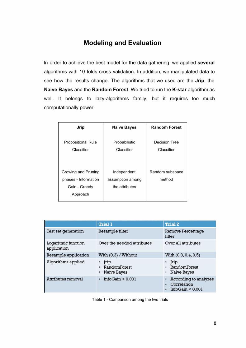
Modeling and Evaluation

In order to achieve the best model for the data gathering, we applied several

algorithms with 10 folds cross validation. In addition, we manipulated data to

see how the results change. The algorithms that we used are the Jrip, the

Naive Bayes and theRandom Forest. We tried to run theK­star algorithm as

well. It belongs to lazy­algorithms family, but it requires too much

computationally power.

Jrip

Propositional Rule

Classifier

Growing and Pruning

phases ­ Information

Gain ­ Greedy

Approach

Naive Bayes

Probabilistic

Classifier

Independent

assumption among

the attributes

Random Forest

Decision Tree

Classifier

Random subspace

method

Table 1 ­ Comparison among the two trials

8

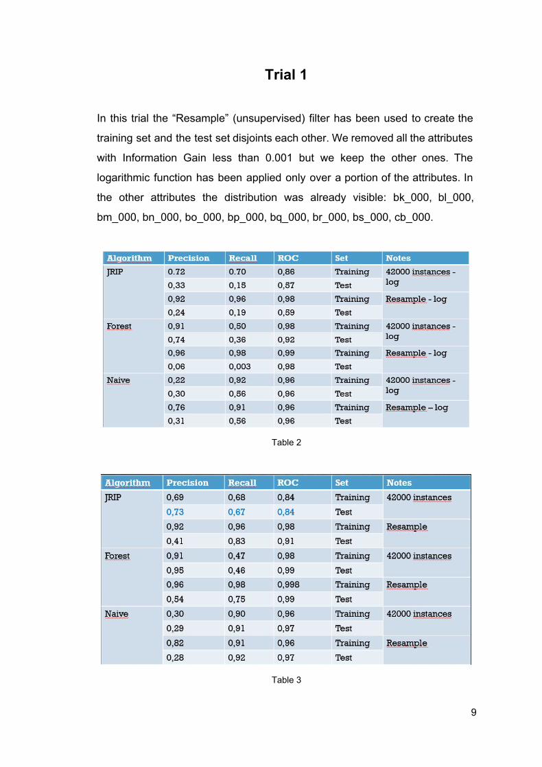
Trial 1

In this trial the “Resample” (unsupervised) filter has been used to create the

training set and the test set disjoints each other. We removed all the attributes

with Information Gain less than 0.001 but we keep the other ones. The

logarithmic function has been applied only over a portion of the attributes. In

the other attributes the distribution was already visible: bk_000, bl_000,

bm_000, bn_000, bo_000, bp_000, bq_000, br_000, bs_000, cb_000.

Table 2

Table 3

9

In the table 2 and table 3 showed above, the results of the three algorithms

executions are reported. The values are referred to the positive class.

The best results was given by the JRip algorithm. It behaved good when no

manipulation has been applied on the data. Random Forest gave a high value

of precision but a not satisfiable value of recall. Naive Bayes gave bad results:

in the case of logarithmic application both of precision and recall values were

very bad, in the other one the recall increased but the precision still had a very

low value.

The Resample affected the results of every algorithm: the JRip and the

Random Forest increased their results on training set but decreased them on

test set; the Naive Bayes increased its results on training set and maintained

the same results on test set.

10

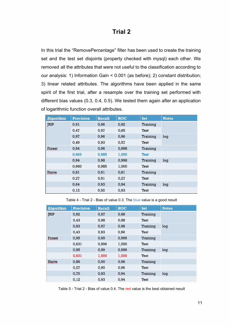
Trial 2

In this trial the “RemovePercentage” filter has been used to create the training

set and the test set disjoints (property checked with mysql) each other. We

removed all the attributes that were not useful to the classification according to

our analysis: 1) Information Gain < 0.001 (as before); 2) constant distribution;

3) linear related attributes. The algorithms have been applied in the same

spirit of the first trial, after a resample over the training set performed with

different bias values (0.3, 0.4, 0.5). We tested them again after an application

of logarithmic function overall attributes.

Table 4 ­ Trial 2 ­ Bias of value 0.3. The blue value is a good result

Table 5 ­ Trial 2 ­ Bias of value 0.4. The red value is the best obtained result

11

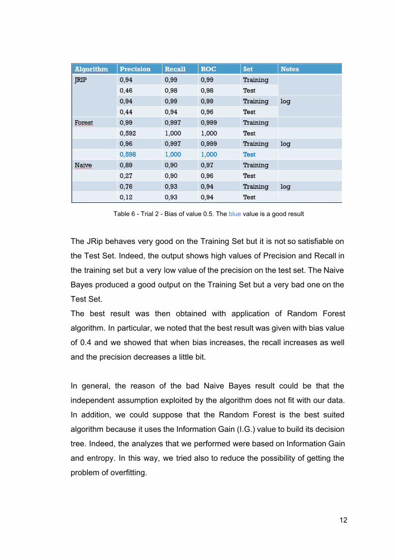
Table 6 ­ Trial 2 ­ Bias of value 0.5. The blue value is a good result

The JRip behaves very good on the Training Set but it is not so satisfiable on

the Test Set. Indeed, the output shows high values of Precision and Recall in

the training set but a very low value of the precision on the test set. The Naive

Bayes produced a good output on the Training Set but a very bad one on the

Test Set.

The best result was then obtained with application of Random Forest

algorithm. In particular, we noted that the best result was given with bias value

of 0.4 and we showed that when bias increases, the recall increases as well

and the precision decreases a little bit.

In general, the reason of the bad Naive Bayes result could be that the

independent assumption exploited by the algorithm does not fit with our data.

In addition, we could suppose that the Random Forest is the best suited

algorithm because it uses the Information Gain (I.G.) value to build its decision

tree. Indeed, the analyzes that we performed were based on Information Gain

and entropy. In this way, we tried also to reduce the possibility of getting the

problem of overfitting.

12

The best model obtained is very good in order to maximize the value of the

recall. Furthermore, the ROC area (Figure 4) has a value of 1.0, which is the

maximum value obtainable.

FIgure 4 ­ Roc Area of value 1.0 as obtained in the trial 2

The ROC curve is a graphical plot that illustrates the performance of a binary

classifier system as its discrimination threshold is varied. The area measures

discrimination, that is, the ability of the test to correctly classify instances.

The greater the area under the curve the better the quality of the model.

Indeed, the top­left area of the curve is an high­precision and high­recall zone.

13