Embed Size (px)
Citation preview
Standard: Distribution Design Manual Vol 5 – Overhead Bare Conductor Distribution Standard Number: HPC-5DC-07-005-2012
SUPERSEDED 04/0
5/201
7 BY
DISTRIB
UTION D
ESIGN R
ULES
HPC-9DJ-
01-0
002-
2015
Page 2 of 139 Print Date: 18/12/2013
© Horizon Power Corporation – Document Number: HPC-5DC-07-0005-2012
Uncontrolled document when printed. Printed copy expires one week from print date. Refer to Document No. for current version.
Document Control
Author Name: Anthony Seneviratne
Position: Standards Engineer
Document Owner
(May also be the Process Owner)
Name: Justin Murphy
Position: Manager Asset Management Services
Approved By * Name: Justin Murphy
Position: Manager Asset Management Services
Date Created/Last Updated February 2014
Review Frequency ** 3 yearly
Next Review Date ** February 2017
* Shall be the Process Owner and is the person assigned authority and responsibility for managing the whole process, end-to-end, which may extend across more than one division and/or functions, in order to deliver agreed business results.
** Frequency period is dependent upon circumstances– maximum is 5 years from last issue, review, or revision whichever is the latest. If left blank, the default shall be 1 year unless otherwise specified.
Revision Control
Revision Date Description
1 14/02/2013 Initial Document
STAKEHOLDERS
The following positions shall be consulted if an update or review is required:
NOTIFICATION LIST The following shall be notified if an update or review is
required
Manager Engineering Services Engineering & Projects
Manager Assets Management Services Operations
SUPERSEDED 04/0
5/201
7 BY
DISTRIB
UTION D
ESIGN R
ULES
HPC-9DJ-
01-0
002-
2015

Page 3 of 139 Print Date 4/05/2017
© Horizon Power Corporation – Document Number: HPC-5DC-07-0005-2012
Uncontrolled document when printed. Printed copy expires one week from print date. Refer to Document No. for current version.
TABLE OF CONTENTS
FOREWORD ............................................................................................................ 10
1 INTRODUCTION ........................................................................................ 11
1.1 General ................................................................................................................ 11
1.2 Pre – Line Design Considerations ........................................................................ 11
2 DESIGN PROCESS .................................................................................... 13
2.1 Determine Design Inputs ...................................................................................... 13
2.2 Selection of Route ................................................................................................ 16
2.3 Selection of Conductor Size and Type .................................................................. 16
2.4 Route Survey and Ground Line Profile ................................................................. 16
2.5 Conductor Stringing Tension and Ruling Span ..................................................... 17
2.6 Selection of Poles and Pole Tops ......................................................................... 17
2.7 Selecting Pole Positions and Pole Top Construction ............................................ 18
2.8 Drawing Line Profile ............................................................................................. 19
2.9 Checking Clearances............................................................................................ 19
2.9.1 Ground Clearance................................................................................................................. 19
2.9.2 Two Circuit Lines .................................................................................................................. 19
2.9.3 Uplift ...................................................................................................................................... 19
2.9.4 Horizontal Clearances .......................................................................................................... 20
2.10 Checking Structure Capacity ................................................................................ 20
2.11 Optimisation of Design .......................................................................................... 21
3 DESIGN PRINCIPLES ................................................................................ 22
3.1 Basic Methodology ............................................................................................... 22
3.2 Security Levels ..................................................................................................... 22
3.3 Design and Service Life ........................................................................................ 22
3.3.1 Minimum Design Wind Return Periods and Security Requirements .................................... 23 3.3.2 Security Level and Failure Containment ............................................................................... 23
3.3.3 Service Life of a Structure .................................................................................................... 24
3.4 Design Principles .................................................................................................. 24
3.4.1 Loading on Structures ........................................................................................................... 25
3.4.2 Risk Management Principles ................................................................................................ 26
3.4.3 Prudent Avoidance Principle ................................................................................................. 26 3.4.3.1 Electro Magnetic Field Exposures ....................................................................................................... 26
3.5 Design Basis ........................................................................................................ 27
3.5.1 Limit States ........................................................................................................................... 27
SUPERSEDED 04/0
5/201
7 BY
DISTRIB
UTION D
ESIGN R
ULES
HPC-9DJ-
01-0
002-
2015
Page 4 of 139 Print Date 4/05/2017
© Horizon Power Corporation – Document Number: HPC-5DC-07-0005-2012
Uncontrolled document when printed. Printed copy expires one week from print date. Refer to Document No. for current version.
3.5.2 Limit State Design ................................................................................................................. 27 3.5.2.1 Limit State Design Loads .................................................................................................................... 28 3.5.2.2 Limit State Design Strength ................................................................................................................. 28 3.5.3 Design Wind Speed .............................................................................................................. 28
3.5.4 Wind Loads ........................................................................................................................... 28
3.5.5 Span Reduction Factor (SRF) .............................................................................................. 30
3.5.6 Temperature ......................................................................................................................... 31
3.6 Strength and Serviceability Limit States ................................................................ 31
3.6.1 Ultimate Strength Limit State ................................................................................................ 31
3.6.2 Serviceability Limit State ....................................................................................................... 31 3.6.3 Strength Reduction Factors .................................................................................................. 31
3.7 Load Combinations ............................................................................................... 32
3.7.1 General ................................................................................................................................. 32 3.7.1.1 Permanent Loads ................................................................................................................................ 33 3.7.2 Load Conditions and Load Factors ....................................................................................... 33 3.7.2.1 Maximum Wind and Maximum Weight ................................................................................................ 33 3.7.2.2 Maximum Wind and Uplift ................................................................................................................... 33 3.7.2.3 Everyday Condition (sustained load) ................................................................................................... 33 3.7.2.4 Serviceability (deflection/damage limit) ............................................................................................... 33 3.7.2.5 Failure Containment Load ................................................................................................................... 33
3.8 Assessing loads on Supports ................................................................................ 35
3.8.1 Intermediate Pole .................................................................................................................. 35
3.8.2 Angle Pole ............................................................................................................................. 35
3.8.3 Termination Pole ................................................................................................................... 35
3.8.4 Load Referral ........................................................................................................................ 35 3.8.5 Bending Moment ................................................................................................................... 35
3.8.6 Pole Strength ........................................................................................................................ 36
3.8.7 List of Symbols ...................................................................................................................... 36
3.8.8 Distribution Worked Example ............................................................................................... 36 3.8.8.1 Ultimate Strength Limit State Assessment (Maximum Wind Load) ..................................................... 39 3.8.8.2 Everyday Load Condition Assessment ................................................................................................ 41 3.8.8.3 Serviceability Condition Assessment................................................................................................... 41 3.8.8.4 Failure Containment Condition Assessment ....................................................................................... 42
4 SUPPORT DESIGN .................................................................................... 44
4.1 Guidelines ............................................................................................................ 44
4.2 Pole Selection ...................................................................................................... 44
4.3 Foundation Design ............................................................................................... 45
4.3.1 Distribution Pole Foundations ............................................................................................... 46
SUPERSEDED 04/0
5/201
7 BY
DISTRIB
UTION D
ESIGN R
ULES
HPC-9DJ-
01-0
002-
2015
Page 5 of 139 Print Date 4/05/2017
© Horizon Power Corporation – Document Number: HPC-5DC-07-0005-2012
Uncontrolled document when printed. Printed copy expires one week from print date. Refer to Document No. for current version.
4.4 Pole Position Guidelines ....................................................................................... 46
4.4.1 Introduction ........................................................................................................................... 46
4.4.2 Designed Pole Alignment ..................................................................................................... 46
4.4.3 General Considerations for Pole Positioning ........................................................................ 47 4.4.3.1 Maximising Number of Customer Services ......................................................................................... 47 4.4.3.2 Street Lighting ..................................................................................................................................... 47 4.4.3.3 Future Extensions ............................................................................................................................... 47 4.4.3.4 Advantages by Positioning .................................................................................................................. 48 4.4.3.5 Earthed Poles ...................................................................................................................................... 49 4.4.3.6 Minimising Deviation Angles ............................................................................................................... 50 4.4.3.7 Proximity to Underground Services ..................................................................................................... 51 4.4.3.8 Road Intersections .............................................................................................................................. 51 4.4.3.9 Driveway Crossovers .......................................................................................................................... 52 4.4.3.10 Easements .......................................................................................................................................... 53 4.4.3.11 Circuit Overhang ................................................................................................................................. 53 4.4.3.12 Stays ................................................................................................................................................... 53 4.4.3.13 Common Lot Boundary Projection ...................................................................................................... 54
5 STAYS ........................................................................................................ 55
5.1 General ................................................................................................................ 55
5.2 Stay Arrangements ............................................................................................... 55
5.3 Stay Formulae ...................................................................................................... 55
5.3.1 Single Stay ............................................................................................................................ 55
5.3.2 Vertical Double Stay ............................................................................................................. 55
5.3.3 Horizontal Double Stay ......................................................................................................... 55 5.3.4 Outrigger Stay ....................................................................................................................... 56
5.3.5 Loads on Poles ..................................................................................................................... 56
5.3.6 Stay Anchorage .................................................................................................................... 56
5.4 List of Symbols ..................................................................................................... 56
5.5 Worked Example .................................................................................................. 57
6 INSULATORS ............................................................................................ 58
6.1 Insulator Design .................................................................................................... 58
6.1.1 Design for Pollution ............................................................................................................... 58
6.1.2 Pins ....................................................................................................................................... 58
6.2 Insulator Strength Limits ....................................................................................... 59
6.3 Insulator Strength Determination .......................................................................... 59
6.3.1 Standard Insulators ............................................................................................................... 60
6.4 Insulator Strength Calculations ............................................................................. 60
6.4.1 Example 1 ............................................................................................................................. 60
SUPERSEDED 04/0
5/201
7 BY
DISTRIB
UTION D
ESIGN R
ULES
HPC-9DJ-
01-0
002-
2015
Page 6 of 139 Print Date 4/05/2017
© Horizon Power Corporation – Document Number: HPC-5DC-07-0005-2012
Uncontrolled document when printed. Printed copy expires one week from print date. Refer to Document No. for current version.
6.4.2 Example 2 ............................................................................................................................. 61
7 CROSS-ARMS ........................................................................................... 63
7.1 Allowable Stress Limits ......................................................................................... 63
7.1.1 Wood Cross-arms ................................................................................................................. 63
7.1.2 Steel Cross-arms .................................................................................................................. 63
7.1.3 Standard Cross-arms ............................................................................................................ 63
7.2 Cross-arm Formulae ............................................................................................. 63
7.2.1 Cross-arm Strength............................................................................................................... 63 7.2.1.1 Intermediate and Angle Cross-arm:..................................................................................................... 63 7.2.1.2 Termination Cross-arm ........................................................................................................................ 63 7.2.2 Loads on Cross-arms ........................................................................................................... 64 7.2.2.1 Intermediate ........................................................................................................................................ 64 7.2.2.2 Angle ................................................................................................................................................... 64 7.2.2.3 Termination ......................................................................................................................................... 65
7.3 List of Symbols ..................................................................................................... 65
7.4 Cross-arm Strength Calculation Examples ........................................................... 66
7.4.1 Calculating Forces ................................................................................................................ 66 7.4.2 Example 2 ............................................................................................................................. 68
8 CONDUCTORS .......................................................................................... 69
8.1 Selection of Conductor ......................................................................................... 69
8.1.1 Electrical Requirements ........................................................................................................ 69 8.1.1.1 Solar Absorption Coefficient ................................................................................................................ 70 8.1.1.2 Wind Velocity ...................................................................................................................................... 70 8.1.1.3 Wind Incident Angle ............................................................................................................................ 70 8.1.1.4 Temperature ........................................................................................................................................ 70 8.1.1.5 Intensity of Solar Radiation ................................................................................................................. 70 8.1.1.6 Ground Reflection Factor .................................................................................................................... 70 8.1.2 Mechanical Requirements .................................................................................................... 70
8.1.3 Environmental Requirements ............................................................................................... 71
8.1.4 Economic Requirements ....................................................................................................... 72 8.1.5 Conductors Currently Installed in the Network ..................................................................... 73
8.1.6 Standard Conductors ............................................................................................................ 74
8.2 Conductor Sag and Tension ................................................................................. 74
8.2.1 Sag and Tension Calculations .............................................................................................. 74
8.2.2 Tension Limits ....................................................................................................................... 74
8.2.3 Conductor Stress and Fatigue .............................................................................................. 75
8.2.4 Span Ratios .......................................................................................................................... 76 8.2.4.1 Wind span ........................................................................................................................................... 76
SUPERSEDED 04/0
5/201
7 BY
DISTRIB
UTION D
ESIGN R
ULES
HPC-9DJ-
01-0
002-
2015
Page 7 of 139 Print Date 4/05/2017
© Horizon Power Corporation – Document Number: HPC-5DC-07-0005-2012
Uncontrolled document when printed. Printed copy expires one week from print date. Refer to Document No. for current version.
8.2.4.2 Weight span ........................................................................................................................................ 77
8.3 Clearance Requirements ...................................................................................... 77
8.3.1 Non Flashover Distances ...................................................................................................... 77
8.3.2 Clearance from Ground ........................................................................................................ 78
8.3.3 Clearance from Structures .................................................................................................... 79
8.3.4 Vertical Spacing of Conductors of Different Circuits ............................................................. 81
8.3.5 Conductors on Same Supports ............................................................................................. 83
8.3.6 Other Clearance .................................................................................................................... 87
8.4 Formulae .............................................................................................................. 87
8.4.1 Ruling Span .......................................................................................................................... 87
8.4.2 Sag ........................................................................................................................................ 87 8.4.2.1 Supports at Same Level: ..................................................................................................................... 87 8.4.2.2 Supports at Different Levels: ............................................................................................................... 87 8.4.2.3 At any Point X: .................................................................................................................................... 87 8.4.3 Tension ................................................................................................................................. 88 8.4.3.1 Set Conditions: .................................................................................................................................... 88 8.4.3.2 Varying Conditions: ............................................................................................................................. 88 8.4.3.3 Checking for Uplift: .............................................................................................................................. 88
8.5 Conductor Ratings ................................................................................................ 90
8.5.1 Conductor Thermal Rating .................................................................................................... 90
8.5.2 Conductor Fault Rating ......................................................................................................... 90 8.5.2.1 Annealing ............................................................................................................................................ 91 8.5.2.2 Maximum Design Operating Temperatures ......................................................................................... 91 8.5.2.3 Design Issues ...................................................................................................................................... 92 8.5.3 Sag/Tension Calculations ..................................................................................................... 92 8.5.3.1 Short bays (Urban) .............................................................................................................................. 92 8.5.3.2 Long Spans(Rural) .............................................................................................................................. 92
8.6 List of Symbols ..................................................................................................... 95
9 VOLTAGE REGULATION .......................................................................... 97
9.1 Voltage Tolerance Limits ...................................................................................... 97
9.1.1 Statutory Voltage Tolerance Limits ....................................................................................... 97 9.1.2 Voltage Drop Criteria ............................................................................................................ 97
9.1.3 Effect of Different Load Cycles ............................................................................................. 98
9.1.4 Voltage Drop Limits for LV Networks .................................................................................... 98
9.1.5 MV Voltage Regulation ......................................................................................................... 99 9.1.5.1 Design Approach ................................................................................................................................. 99 9.1.5.2 Computer Modelling ............................................................................................................................ 99 9.1.5.3 Voltage Control Equipment ................................................................................................................. 99 9.1.5.4 Calculating MV Voltage Drop ............................................................................................................ 100
SUPERSEDED 04/0
5/201
7 BY
DISTRIB
UTION D
ESIGN R
ULES
HPC-9DJ-
01-0
002-
2015
Page 8 of 139 Print Date 4/05/2017
© Horizon Power Corporation – Document Number: HPC-5DC-07-0005-2012
Uncontrolled document when printed. Printed copy expires one week from print date. Refer to Document No. for current version.
9.1.5.5 Worked Example ............................................................................................................................... 101
9.2 Line Drop Compensators (LDC) ......................................................................... 102
10 LV NETWORK DESIGN ........................................................................... 105
10.1 Introduction ......................................................................................................... 105
10.1.1 General ............................................................................................................................... 105
10.1.2 Primary Aim ........................................................................................................................ 105 10.1.3 Challenge for Network Designers ....................................................................................... 105
10.1.4 Use of Computer Packages ................................................................................................ 105
10.1.5 Aspects of Electrical Design ............................................................................................... 106
10.2 Determination of Recommended Load Demand Values ..................................... 106
10.2.1 Introduction ......................................................................................................................... 106
10.2.2 Effect of Load Diversity on Maximum Demand .................................................................. 107
10.2.3 Determination of Design Load Demand Values ................................................................. 107
10.2.4 Application of After Diversity Maximum Demand (ADMD) ................................................. 108
10.2.5 Residential Load ADMDs .................................................................................................... 109 10.2.6 Non-Residential Load Demands ......................................................................................... 109
10.2.7 Residential Lot Classification .............................................................................................. 109
10.2.8 LV Conductor Selection Guidelines .................................................................................... 110
10.2.9 LV Conductor Data Table ................................................................................................... 110
10.2.10 Selection of LV Feeder Routes ........................................................................................... 110 10.2.10.1 Proximity to Loads ............................................................................................................................. 110 10.2.10.2 Utilisation/Loading ............................................................................................................................. 111 10.2.10.3 Typical Lengths ................................................................................................................................. 111 10.2.10.4 Interconnection with Other Feeders .................................................................................................. 111 10.2.10.5 Pole Positioning and Alignment ......................................................................................................... 111 10.2.10.6 Other Considerations ........................................................................................................................ 111
10.3 Voltage Drops and Line Currents in LV Feeders ................................................. 112
10.3.1 General ............................................................................................................................... 112
10.3.2 Effect of Load Unbalance ................................................................................................... 112
10.3.3 Voltage Drops/Line Currents in Meshed Networks ............................................................. 112
11 FAULT LEVEL ......................................................................................... 114
11.1 Introduction ......................................................................................................... 114
11.2 Equipment Rating ............................................................................................... 114
11.3 Fault Calculation ................................................................................................. 115
11.4 Formulae ............................................................................................................ 115
11.4.1 Ohmic Impedance ............................................................................................................... 116 11.4.2 Per Cent Impedance ........................................................................................................... 116
SUPERSEDED 04/0
5/201
7 BY
DISTRIB
UTION D
ESIGN R
ULES
HPC-9DJ-
01-0
002-
2015
Page 9 of 139 Print Date 4/05/2017
© Horizon Power Corporation – Document Number: HPC-5DC-07-0005-2012
Uncontrolled document when printed. Printed copy expires one week from print date. Refer to Document No. for current version.
11.4.3 Per Unit Impedance ............................................................................................................ 116
11.4.4 Worked Example using Per Unit method ............................................................................ 116 11.4.5 Worked example using MVA method ................................................................................. 119
11.4.6 Zone Substation Fault Levels ............................................................................................. 120
12 INSULATION COORDINATION ............................................................... 121
12.1 Introduction ......................................................................................................... 121
12.2 Design for Power Frequency Overvoltages ......................................................... 122
12.3 Design for Impulse voltages................................................................................ 122
12.3.1 Lightning ............................................................................................................................. 122 12.3.1.1 Direct Strikes ..................................................................................................................................... 122 12.3.1.2 Induced Strokes ................................................................................................................................ 126 12.3.2 Current ................................................................................................................................ 127 12.3.3 Surge Impedance................................................................................................................ 127
12.3.4 Lightning Protection using Surge Arresters ........................................................................ 127
12.3.5 Selection of Surge Arresters ............................................................................................... 127
12.3.6 Impulse Flashover of Adjacent Insulators ........................................................................... 130
13 STREET LIGHTING .................................................................................. 131
13.1 Policy .................................................................................................................. 131
13.2 Asset Hierarchy .................................................................................................. 131
13.3 Lighting Categories and Application .................................................................... 131
13.4 Lighting Design Basis ......................................................................................... 133
13.4.1 Selection of Lamp Types .................................................................................................... 133
13.4.2 Luminaire Technical Requirements .................................................................................... 133
13.4.3 Design Considerations ........................................................................................................ 133
13.4.4 Minimum Lighting Performance Requirements .................................................................. 134
13.4.5 Lamp Poles ......................................................................................................................... 134 13.4.6 Electrical Protection of Street Lights ................................................................................... 136 APPENDIX A – REVISION INFORMATION ....................................................................................................... 138 APPENDIX B – RELATED INFORMATION ........................................................................................................ 139 SUPERSEDED 0
4/05/2
017
BY
DISTRIB
UTION D
ESIGN R
ULES
HPC-9DJ-
01-0
002-
2015
Page 10 of 139 Print Date 4/05/2017
© Horizon Power Corporation – Document Number: HPC-5DC-07-0005-2012
Uncontrolled document when printed. Printed copy expires one week from print date. Refer to Document No. for current version.
FOREWORD This volume is one in a series of five volumes, which together, form the Horizon Power Distribution Design Manual. The DDM is intended to be a comprehensive reference manual for distribution design work carried out by professional engineers and technical support staff.
The five volumes are:
Volume 1: Quality of Electricity Supply
Volume 2: Low Voltage Aerial Bundled Cable
Volume 3: Supply to Large Customer Installations
Volume 4: Underground Residential Distribution (URD)
Volume 5: Overhead Bare Conductor Distribution
The DDM will also serve to initiate "newcomers" to distribution work in Horizon Power without them having to start from scratch. It serves to establish "standards" for design work to ensure that we get the best value from our facilities - not only in terms of initial cost, but also in terms of component availability, length of service life and cost-effective maintenance. In addition to this, the DDM will also serve as a teaching aid for courses run by Horizon Power.
This volume describes the engineering process involved in designing and providing electricity supplies using bare overhead conductor.
It describes the design process in detail, making use of standardised design information for use with routine work.
SUPERSEDED 04/0
5/201
7 BY
DISTRIB
UTION D
ESIGN R
ULES
HPC-9DJ-
01-0
002-
2015
Page 11 of 139 Print Date 4/05/2017
© Horizon Power Corporation – Document Number: HPC-5DC-07-0005-2012
Uncontrolled document when printed. Printed copy expires one week from print date. Refer to Document No. for current version.
1 INTRODUCTION
1.1 General This document describes the engineering process involved in designing distribution overhead power lines. These lines typically originate from Zone substations as Medium Voltage lines and are stepped down to Low Voltage through distribution transformers. Low Voltage overhead power lines then transmit power from transformers to customer installations. Some customers are supplied directly from the Medium Voltage network.
Overhead Power lines account for a significant proportion of Horizon Power's networks. These assets involve large amounts of capital expenditure, both by Horizon Power and customers. Also, these lines need to be properly designed and constructed and it is imperative that a high level of engineering input is put into their designs, particularly because these lines may be built in cyclonic areas. Effort expended here could avoid unnecessary expenses for Horizon Power and customers and ensure that the customer's requirements and all of Horizon Power's requirements are catered for.
Each overhead line requires different design considerations, configurations, layouts, etc. As such, there may be many different ways to approach a design.
The information contained in this manual will assist the designer to develop a structured design approach, and ensure that the optimum line configuration is selected at all times.
1.2 Pre – Line Design Considerations There are certain basic requirements that have to be considered when designing overhead distribution power lines. These requirements fall within the broader National Standards and Guidelines (e.g. AS 7000). This manual has been put in place to facilitate the development of innovative project designs that will aim at:
(a) Reduced cost to customers; (b) Reduced Life Cycle ( Maintenance) costs; (c) Greater durability with due consideration to location in a cyclonic areas; (d) Safety of workers and the General Public; (e) Environmental Compatibility; (f) Electromagnetic Field Compatibility; (g) Favourable public acceptance ( aesthetics); and (h) Increased network safety and reliability
When the requirement for a line has been established, the following factors need to be considered before the design can commence. They are:
a) Potential number of Customers and total load; b) Estimation of potential load growth; c) Availability/ and or requirement for interconnections; d) Selection of Voltage for line operation; e) Size and location of loads (Bulk supply, transformers) f) Selection of Route g) Length of line h) Life Cycle costs
SUPERSEDED 04/0
5/201
7 BY
DISTRIB
UTION D
ESIGN R
ULES
HPC-9DJ-
01-0
002-
2015

Page 12 of 139 Print Date 4/05/2017
© Horizon Power Corporation – Document Number: HPC-5DC-07-0005-2012
Uncontrolled document when printed. Printed copy expires one week from print date. Refer to Document No. for current version.
The capacity (load) to be carried by the power line during its lifetime together with voltage drop and fault rating considerations will dictate the size and type of conductor to be used. The line design process is discussed in Chapter 2.
SUPERSEDED 04/0
5/201
7 BY
DISTRIB
UTION D
ESIGN R
ULES
HPC-9DJ-
01-0
002-
2015
Page 13 of 139 Print Date 4/05/2017
© Horizon Power Corporation – Document Number: HPC-5DC-07-0005-2012
Uncontrolled document when printed. Printed copy expires one week from print date. Refer to Document No. for current version.
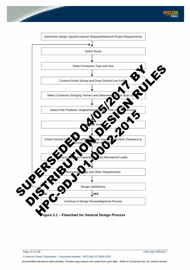
2 DESIGN PROCESS Typical steps in an overhead distribution line design are shown below. The actual steps and their sequence will depend upon the individual project and the context in which the design is performed.
The process is iterative, with the designer making some initial assumptions, e.g. as to pole height and size, which may later need to be adjusted as the design is checked and gradually refined. The optimum arrangement that meets all constraints is required as the final outcome. Horizon Power uses overhead line simulation software to aid the design process.
The generalised design process is shown in Figure 2.1.
2.1 Determine Design Inputs Prior to commencing design, it is important to collect and document all relevant design inputs. This may include:
a) planning reports, concept, specification or customer request for supply initiating the project;
b) load details, disturbing loads etc; c) special requirements of customers or stakeholders (e.g. supply reliability); d) system planning requirements; e) information about possible future stages or adjacent developments, road
widening or other; f) applicable relevant standards and statutory requirements; g) co-ordination with other utilities - 'Dial Before You Dig' results h) co-ordination with road lighting design; i) survey plans or base maps; j) any site constraints identified and k) environmental factors (as elaborated below)
The designer should take into consideration the environmental factors which could influence the design of the supply arrangement, e.g. selection of and location of equipment, etc.
For example, suppose an overhead MV line is to be constructed to supply a customer remote from a zone substation, and the line route traverses an area of high lightning activity. It would seem prudent for the designer to include an earth-wire system to shield the conductors, in the line design, even though this is not normal practice for distribution lines.
Similar considerations should apply for lines or installations close to the coast, which are subjected to high salt-pollution levels. High pollution insulators may be incorporated in the line design.
Consideration must be given to the location of the equipment or the environment the equipment is to operate in. For example, a pole top transformer may not be entirely suitable for use outside a cement plant or quarry, where the build up of fly-ash or dust on insulators may lead to nuisance tripping or a disproportionately high level of maintenance. Others include mines sites, with open air blasting, etc.
SUPERSEDED 04/0
5/201
7 BY
DISTRIB
UTION D
ESIGN R
ULES
HPC-9DJ-
01-0
002-
2015
Page 14 of 139 Print Date 4/05/2017
© Horizon Power Corporation – Document Number: HPC-5DC-07-0005-2012
Uncontrolled document when printed. Printed copy expires one week from print date. Refer to Document No. for current version.
Consideration shall also be given to:
• Cultural Heritage and Native Title;
• Environmental approvals for clearing or removal of native vegetation; and
• Siting of Substations with respect to Noise Control.
Current statutory processes require a range of approvals to be obtained prior to commencement of works. Due to the time taken to obtain these approvals, these issues must be considered at the commencement of a project.
As per the Western Australian Distribution Connections Manual (WADCM Section 6.12) environmental and heritage impacts must be investigated and managed by the applicant for power supply and their agent. Issues may include but are not limited to the following:
a) Aboriginal heritage sites and objects of suspected aboriginal origin;
b) Acid sulphate soils;
c) Bio-security weeds, pests and disease spread (e.g. dieback disease);
d) Declared rare flora and threatened ecological communities;
e) Dust;
f) Erosion;
g) Land entry permits;
h) Native title;
i) Noise;
j) Protected wetlands;
k) Vegetation clearing permits; and
l) Waste management including controlled waste.
The design should be 'traceable' back to a set of design inputs. Persons other than the original designer should be able to review the design and see why it was done a certain way.
SUPERSEDED 04/0
5/201
7 BY
DISTRIB
UTION D
ESIGN R
ULES
HPC-9DJ-
01-0
002-
2015
Page 15 of 139 Print Date 4/05/2017
© Horizon Power Corporation – Document Number: HPC-5DC-07-0005-2012
Uncontrolled document when printed. Printed copy expires one week from print date. Refer to Document No. for current version.
Determine Design Inputs/Customer Requests/Network Project Requirements
Select Route
Select Conductor Type and Size
Conduct Route Survey and Draw Ground Line Profile
Select Conductor Stringing Tension and Determine Typical Span Length
Select Pole Positions, Heights/Strengths and Pole Top Construction
Draw Line Profile
Check Vertical Clearances/Uplift/Horizontal clearances / Check Clearance to structures and other obstacles
Check Structure Capacity Matches Mechanical Loads
Nominate Fittings and Other Requirements
Design Satisfactory
NO YES
Continue to Design Review/Approval Process
Figure 2.1 – Flowchart for General Design Process
SUPERSEDED 04/0
5/201
7 BY
DISTRIB
UTION D
ESIGN R
ULES
HPC-9DJ-
01-0
002-
2015
Page 16 of 139 Print Date 4/05/2017
© Horizon Power Corporation – Document Number: HPC-5DC-07-0005-2012
Uncontrolled document when printed. Printed copy expires one week from print date. Refer to Document No. for current version.
2.2 Selection of Route Ideally, the line route should be as short and straight as possible in order to minimise costs, minimise stays and have a tidy appearance. However, some other factors that need to be taken into account are:
a) Land issues, ease of acquisition, rights over private lands etc.; b) Ease of obtaining necessary approvals; c) Stakeholder considerations and acceptance; d) Vegetation clearing, environmental and visual impact, EMF impact; e) Access for construction, maintenance and operations; f) Ease of servicing all lots for Low Voltage Lines; g) Compatibility with future development; h) Waterways, parks and natural habitat; and i) Terrain suitability and ground conditions (excavation, pole foundation etc.)
2.3 Selection of Conductor Size and Type Selection of conductors is covered in section 8.1. Factors influencing selection include:
a) Load current and whether the line is 'backbone' or a spur; b) Line voltage and voltage profile along the line; c) Fault levels and line rating; d) Environmental conditions – ambient temperature, vegetation, wildlife,
pollution or salt spray; e) Compatibility with existing adjacent electrical infrastructure; f) Required span lengths and stringing tension; and g) Future requirements with respect to distribution system planning.
2.4 Route Survey and Ground Line Profile A ‘line route survey’ is carried out to determine:
a) Details of existing electricity infrastructure; b) Terrain and site features, e.g. trees, access tracks, fences, gullies; and c) Ground line rise and fall along the route.
Ground line profiling may not be necessary for minor projects in urban areas where the ground is reasonably level or has a consistent slope throughout and there are no on site obstructions.
The designer can check worst case ground clearances by deducting the sag in the span from the height of the supports at either end by taking the following measurements:
a) Conductor temperature b) Conductor size/type c) Ambient temperature d) Conductor attachment point with respect to ground level e) Strain points
SUPERSEDED 04/0
5/201
7 BY
DISTRIB
UTION D
ESIGN R
ULES
HPC-9DJ-
01-0
002-
2015

Page 17 of 139 Print Date 4/05/2017
© Horizon Power Corporation – Document Number: HPC-5DC-07-0005-2012
Uncontrolled document when printed. Printed copy expires one week from print date. Refer to Document No. for current version.
However, ground line profiling is essential where:
1) Poles have to be positioned along an undulating traverse; 2) There is a 'hump' or change in gradient in the ground at mid span; 3) Outside of urban areas where spans are comparatively long-say in excess
of 80 m; 4) The designer has doubts about the adequacy of required clearances; and 5) Where uplift on poles is suspected.
The equipment used to obtain measurements will depend on the complexity of the project. For many distribution lines, a simple electronic distance measuring device and inclinometer are adequate. Elsewhere, use of a high end GPS unit or LiDAR may be warranted. The route is broken up into segments, typically corresponding with 'knee points' or changes in gradient. Slope distance and inclination measurements for each segment can be converted to chainage and reduced level (RL) values to facilitate plotting as follows:
Software packages can be used to plot survey data. Apart from the ground line, various features and stations must be shown, including existing poles, gullies, fences, obstacles, roadways. A clearance line is then drawn offset from the ground line, according to the minimum vertical clearances that apply (refer chapter 8).
2.5 Conductor Stringing Tension and Ruling Span Refer to Chapter 8 for guidance on selecting a suitable stringing tension and Ruling Span.
2.6 Selection of Poles and Pole Tops Typical pole sizes are presented in Table 4.7. When selecting poles, potential future sub-circuits and streetlight mounting must be considered, if these are identified / known during the design phase.
Apart from spanning and angular limitations, selecting a suitable pole top configuration should take in to account:
1) Life cycle suitability; 2) Reliability; 3) Suitability for the environment (vegetation, wild life, salt and/or industrial
pollution levels); and 4) Ease of construction and maintenance.
Horizontal (flat) construction has the advantage of reduced pole height at the expense of a wider line and corresponding broader easement width.
Flat configurations are preferred in areas frequented by birds. For higher risk spans increasing conductor separation can reduce conductor flashover due to bird impact. Attaching bird diverters on conductors is also effective as a visual warning to birds.
Delta pin configuration provides for both horizontal and vertical separation and helps reduce conductor clashing.
SUPERSEDED 04/0
5/201
7 BY
DISTRIB
UTION D
ESIGN R
ULES
HPC-9DJ-
01-0
002-
2015

Page 18 of 139 Print Date 4/05/2017
© Horizon Power Corporation – Document Number: HPC-5DC-07-0005-2012
Uncontrolled document when printed. Printed copy expires one week from print date. Refer to Document No. for current version.
Overall, more compact pole top configurations are less visually obstructive. It is best to keep to reasonably consistent configurations to maintain visual amenity as well as maintain spanning capability and ease of conductor phasing.
2.7 Selecting Pole Positions and Pole Top Construction Refer to section 4.4 for pole positioning guidelines.
Firstly, position poles along the route at any key or constrained locations.
Next determine the maximum span length that can be achieved over flat ground given the attachment heights on poles, the sag at the nominated stringing tension and the required ground clearance. Also check the spanning capability of the pole top constructions to be used. Position poles along the route so that this spacing is not exceeded. If there are gullies between poles, the spacing can be increased and if there are 'humps' mid-span, span lengths can be reduced.
Strain Points, Pole Details and Pole Top Constructions have to be determined. Strain point locations need to be determined:
1) To isolate electrically different circuits. 2) To keep very short spans or very long spans mechanically separate, such
that all spans in a strain section are of similar length (no span less than half or more than double the ruling span length, and on tight-strung lines, the longest span not more than double the shortest span). Failure to limit span variance can cause excess sagging in longest span at higher design temperature loadings.
3) To isolate critical spans, e.g. spans over a river, major highway or railway line, to help facilitate repairs or maintenance.
4) On line deviation angles too great for intermediate constructions, e.g. Cross-arms with pin insulators.
5) At locations where there are uplift forces on poles. 6) At intervals of approximately 10 spans or so.
The following points also must be considered:
1) Strain section length limitation will be favourable if a line is affected by wires brought down in a storm. Also, the length of conductor on a drum may be a consideration.
2) Span lengths within the strain section must be reasonably similar and poles and pole top construction used must be reasonably consistent, as this gives the line a tidy appearance.
3) When nominating suitable pole top constructions for intermediate poles, adequate capacity must be available for the deviation angle at each site.
4) Pole strengths and foundation types/sinking depths must be nominated as a first pass, as these may need to be amended later once tip loads are determined. Stronger poles will be required at terminations and on large deviation angles. Pole sinking depths can be determined in accordance with Table 4.7.
SUPERSEDED 04/0
5/201
7 BY
DISTRIB
UTION D
ESIGN R
ULES
HPC-9DJ-
01-0
002-
2015

Page 19 of 139 Print Date 4/05/2017
© Horizon Power Corporation – Document Number: HPC-5DC-07-0005-2012
Uncontrolled document when printed. Printed copy expires one week from print date. Refer to Document No. for current version.
2.8 Drawing Line Profile Overhead line simulation software program can be used to draw the line profile.
Poles are shown to scale on the profile, with marks placed at the support points for each circuit.
The conductors are shown by selected conductor type, stringing tension and ruling span linking two support points for the circuit. Different conductor profiles can be generated to depict the varying temperature conditions such as the maximum design temperature, everyday temperature, cold or uplift conditions.
2.9 Checking Clearances
2.9.1 Ground Clearance If the line profile screen shows that there is insufficient ground clearance (refer to clause 8.3.2) the designer may need to:
• Reduce span length;
• Increase stringing tension;
• Increase pole height; and
• Adjust pole positions to try to fit in better with the terrain.
2.9.2 Two Circuit Lines Where there are spans with an upper circuit and a lower circuit, the inter circuit clearance should be checked. (Refer to section 8.3).
2.9.3 Uplift Poles at the bottom of a hill or in a gully are prone to uplift. Under cold conditions, the conductors heading up the slope will become tight and pull upward on structures, causing damage.
Uplift is generally not a problem if it is on one side of the structure only and offset on the opposite side by a downward force, as may occur with a line with successive spans running down a steep slope. However, if on both sides of an intermediate structure such as a suspension or pin construction, it needs to be addressed. Possible solutions include:
a) Changing the pole top construction to a termination type; b) Moving the pole to a different location; c) Reducing stringing tension; d) Increasing pole height; and e) Reducing heights of adjacent poles subject to having adequate ground
clearance.
Uplift is managed in different ways in line design software packages. It is important to verify how to conduct this important check.
SUPERSEDED 04/0
5/201
7 BY
DISTRIB
UTION D
ESIGN R
ULES
HPC-9DJ-
01-0
002-
2015
Page 20 of 139 Print Date 4/05/2017
© Horizon Power Corporation – Document Number: HPC-5DC-07-0005-2012
Uncontrolled document when printed. Printed copy expires one week from print date. Refer to Document No. for current version.
2.9.4 Horizontal Clearances The designer should check that there are adequate horizontal clearances between the line and any nearby structures (e.g. flag poles, buildings, bridge columns, streetlight columns) or embankments. (Refer to clause 8.3.3) These clearances should be checked for both - (a) the no wind condition and (b) the blowout conditions.
Ways of addressing horizontal clearance problems include:
a) Increasing conductor tension; b) Reducing span length; c) Relocating poles to a different alignment; d) Ensuring that poles are placed in line with any objects, so that there is nil
blow out; e) Using different pole top constructions, e.g. vertical construction; f) Using insulated cables or underground cables rather than bare conductors
where feasible; g) Relocating objects affected, where feasible, e.g. Streetlights; and h) Increasing line height to skip over the object, where feasible.
2.10 Checking Structure Capacity Tip load calculations must be undertaken for each of the poles, in the line. Forces exerted by conductors are detailed in Chapter 3. Conductors attached significantly below the tip have their applied force scaled down proportionately. Forces are added as vectors, not scalar quantities unless in the same direction.
The applied tip load is then compared with the capacity of the pole.
Where the pole has more than adequate strength, the designer may investigate whether it is feasible to drop down to a smaller size, e.g. from a 24 kN to an 16 kN pole. This may mean an adjustment to sinking depth as a consequence, which will affect the profile marginally.
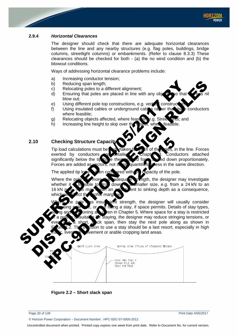
Where the pole has insufficient strength, the designer will usually consider increasing pole size, or else fitting a stay, if space permits. Details of stay types, sizing and positioning are given in Chapter 5. Where space for a stay is restricted or a pole is unsuitable for staying, the designer may reduce stringing tensions, or even use a short, slack span, then stay the next pole along as shown in Figure 2.2. The decision to use a stay should be a last resort, especially in high traffic, livestock movement or arable cropping land areas.
Figure 2.2 – Short slack span
SUPERSEDED 04/0
5/201
7 BY
DISTRIB
UTION D
ESIGN R
ULES
HPC-9DJ-
01-0
002-
2015

Page 21 of 139 Print Date 4/05/2017
© Horizon Power Corporation – Document Number: HPC-5DC-07-0005-2012
Uncontrolled document when printed. Printed copy expires one week from print date. Refer to Document No. for current version.
2.11 Optimisation of Design The design process is iterative. The initial first-pass design is 'tweaked' repeatedly until it complies with all technical (standards and regulations) and stakeholder requirements and is optimal in terms of cost, reliability and practicality for construction, maintenance and operations.
SUPERSEDED 04/0
5/201
7 BY
DISTRIB
UTION D
ESIGN R
ULES
HPC-9DJ-
01-0
002-
2015
Page 22 of 139 Print Date 4/05/2017
© Horizon Power Corporation – Document Number: HPC-5DC-07-0005-2012
Uncontrolled document when printed. Printed copy expires one week from print date. Refer to Document No. for current version.
3 DESIGN PRINCIPLES
3.1 Basic Methodology The design methodology involves the development of a suite of appropriate structures, insulation and constructions for use at the various voltage levels to comply with AS 7000 - Overhead Line Design (Detailed Procedures). The overhead line has to perform with suitable levels of reliability and security for the weather related loads expected in the region it is installed for the entirety of its intended life.
3.2 Security Levels All overhead lines should be designed for a selected security level relevant to the lines importance to the system (including consideration of system redundancy), its location and exposure to climatic conditions, and with due consideration for public safety and design working life.
AS 7000 (Chapter 6) provides a framework to evaluate and select standard designs to suit a relevant security level appropriate to a particular line, line construction class or line type.
The security levels are defined below:
Level 1 Applicable to overhead lines where collapse of the line may be tolerable with respect to social and economic consequences. (Normal distribution lines).
Level 2 Applicable to overhead lines where collapse of the line would cause negligible danger to life and property and alternative arrangements can be provided if loss of support services occurs. (Higher security distribution lines and normal transmission lines).
Level 3 Applicable to overhead lines where collapse of the line, would cause unacceptable danger to life or significant economic loss to the community and sever vital post disaster services. (Higher security transmission lines).
3.3 Design and Service Life The design life, or target nominal service life expectancy of the line is dependent on its exposure to a number of variable factors such as solar radiation, temperature, precipitation, wind and seismic effects.
The service life of an overhead line is the period over which it will continue to serve its intended purpose safely, without undue maintenance or repair disproportionate to its cost of replacement and without exceeding any specified serviceability criteria.
The structural supports must be able to withstand the ultimate design loadings without failure, during this period. This may include providing allowance for a reducing load factor over time due to progressive degradation such as soft rot in timber poles and corrosion in steel poles.
SUPERSEDED 04/0
5/201
7 BY
DISTRIB
UTION D
ESIGN R
ULES
HPC-9DJ-
01-0
002-
2015
Page 23 of 139 Print Date 4/05/2017
© Horizon Power Corporation – Document Number: HPC-5DC-07-0005-2012
Uncontrolled document when printed. Printed copy expires one week from print date. Refer to Document No. for current version.
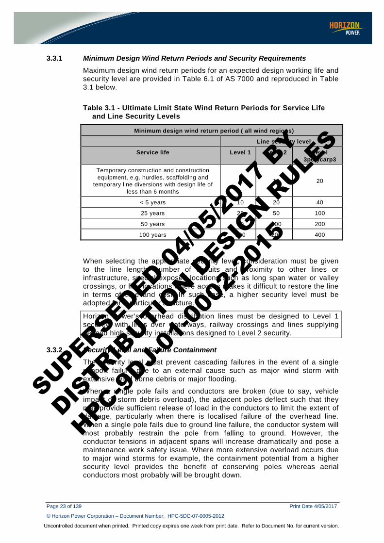
3.3.1 Minimum Design Wind Return Periods and Security Requirements Maximum design wind return periods for an expected design working life and security level are provided in Table 6.1 of AS 7000 and reproduced in Table 3.1 below.
Table 3.1 - Ultimate Limit State Wind Return Periods for Service Life
and Line Security Levels
Minimum design wind return period ( all wind regions)
Line security level
Service life Level 1 Level 2 Level 3polycarp3
Temporary construction and construction equipment, e.g. hurdles, scaffolding and
temporary line diversions with design life of less than 6 months
5 10 20
< 5 years 10 20 40
25 years 25 50 100
50 years 50 100 200
100 years 100 200 400
When selecting the appropriate security level, consideration must be given to the line length, number of circuits and proximity to other lines or infrastructure, special exposed locations such as long span water or valley crossings, or line locations where access makes it difficult to restore the line in terms of time and cost. In such case, a higher security level must be adopted for a particular structure.
Horizon Power’s overhead distribution lines must be designed to Level 1 security, with lines over waterways, railway crossings and lines supplying defined high security installations designed to Level 2 security.
3.3.2 Security Level and Failure Containment The security level must prevent cascading failures in the event of a single support failure due to an external cause such as major wind storm with extensive wind borne debris or major flooding.
When a single pole fails and conductors are broken (due to say, vehicle impact or storm debris overload), the adjacent poles deflect such that they may provide sufficient release of load in the conductors to limit the extent of damage, particularly when there is localised failure of the overhead line. When a single pole fails due to ground line failure, the conductor system will most probably restrain the pole from falling to ground. However, the conductor tensions in adjacent spans will increase dramatically and pose a maintenance work safety issue. Where more extensive overload occurs due to major wind storms for example, the containment potential from a higher security level provides the benefit of conserving poles whereas aerial conductors most probably will be brought down.
SUPERSEDED 04/0
5/201
7 BY
DISTRIB
UTION D
ESIGN R
ULES
HPC-9DJ-
01-0
002-
2015
Page 24 of 139 Print Date 4/05/2017
© Horizon Power Corporation – Document Number: HPC-5DC-07-0005-2012
Uncontrolled document when printed. Printed copy expires one week from print date. Refer to Document No. for current version.
On distribution overhead pole lines, pole deflection (usually rotational and lateral or longitudinal) combined with partial foundation deformation, will occur when abnormal longitudinal loads are applied.
As per AS 7000, on poles subject to tension such as termination poles, failure containment conditions must be considered during design.
3.3.3 Service Life of a Structure The service life of a structure (e.g. pole) is the period in years over which it will continue to serve its intended purpose safely, without undue maintenance or repair disproportionate to its cost of replacement and without exceeding any specified serviceability criteria. This recognises that cumulative deterioration of the structure over time will occur, due to ‘wear and tear’ or environmental effects. Therefore, in order to maintain structural integrity within adequate design margins, adequate maintenance and possible minor repairs will be required from time to time to maintain the structure in a safe and useable condition over its service life.
Structures and fittings located close to the sea typically within 1.0 km from the sea will be subjected to more severe exposure and would normally require either special protection or a shorter service life. Experience in these coastal regions suggests that metallic fittings will be the weakest link over time and may need to be replaced more than once during the service life of the structure.
Horizon Power is committed to using steel poles on new lines and when replacing poles on existing lines. The above ground service life of steel poles is expected to be 50 years, using hot dip galvanizing that provides a minimum average zinc coating mass of 400 g/m2, in line with Table D2 of AS 7000. By using 600 g/m2, of zinc galvanizing on steel, the above ground service life can be extended to 75 years.
Added protection will be required for the portion of the steel pole embedded in the ground and just above ground line to prevent degradation and loss of strength due to corrosion.
3.4 Design Principles The main technical aspects in the design of overhead lines are ensuring that:
• the mechanical load forces do not exceed the strength of structures or other components, and
• there are adequate clearances – between the conductors and the ground or from other objects in the vicinity of the line, as well as between the various phase conductors and circuits themselves so that clashing does not occur.
The line must comply with these requirements over the full design range of weather and other load conditions that could reasonably encountered – when the line is cold and taut, when at its maximum design temperature and consequently when conductor sag is at a maximum, and under maximum wind conditions. The load conditions to be considered for Horizon Power lines are set out in the following sections, where applicable wind pressures, temperatures and load factors are provided.
SUPERSEDED 04/0
5/201
7 BY
DISTRIB
UTION D
ESIGN R
ULES
HPC-9DJ-
01-0
002-
2015

Page 25 of 139 Print Date 4/05/2017
© Horizon Power Corporation – Document Number: HPC-5DC-07-0005-2012
Uncontrolled document when printed. Printed copy expires one week from print date. Refer to Document No. for current version.
3.4.1 Loading on Structures The loads on a structure consist of three mutually perpendicular systems of load acting vertical, normal to the direction of line, and parallel to the direction of the line. These loads can be described as:
• Vertical load
• Transverse load
• Longitudinal load
Vertical loads Vertical loads include the weight of conductors, earth wires, cross arms and pole mounted plant such as transformers.
Transverse loads Transverse loads are caused by wind on conductor and structure and horizontal tension from deviation angle in the line.
Longitudinal loads Longitudinal loads are caused by difference in conductor tension on either side of termination structures, adjacent spans being of different lengths and an abnormal (broken wire) load on the structure.
Figure 3.1 - Forces on Poles
SUPERSEDED 04/0
5/201
7 BY
DISTRIB
UTION D
ESIGN R
ULES
HPC-9DJ-
01-0
002-
2015
Page 26 of 139 Print Date 4/05/2017
© Horizon Power Corporation – Document Number: HPC-5DC-07-0005-2012
Uncontrolled document when printed. Printed copy expires one week from print date. Refer to Document No. for current version.
3.4.2 Risk Management Principles The layout design process should include the identification and assessment of risks associated with the construction, maintenance and operation of the proposed line leading to the evaluation and implementation of risk treatment options which ensure that the residual risk is acceptable to Horizon Power.
3.4.3 Prudent Avoidance Principle Where potential risks with unproven consequences are involved, a prudent avoidance approach is recommended. This essentially means doing what can be done without undue inconvenience and at modest expense to avert a possible risk.
3.4.3.1 Electro Magnetic Field Exposures Due to the need to provide supply to customers, the options available to designers in locating distribution lines and substations are limited. Distribution lines, by their very nature and function are normally located in road reserves to provide supply to customers on both sides of the road. Where practicable to reduce electromagnetic exposures: distribution lines should be:
a) Located on the opposite side of the road from areas such as schools, kindergartens, child-care centres and the like.
b) Sited away from the walls of multi storey buildings or areas where children congregate.
c) Located on the side of the road bordered by open spaces where applicable.
Prudent design options to reduce electromagnetic exposures from distribution lines include but not limited to:
i. Use of aerial bundled cables for low voltage reticulation to provide more effective field cancellation
ii. Balancing of load across all phases to reduce neutral currents iii. Adopt a low reactance (RWB/BWR) phasing when current flow in both
circuits is in the same direction for new double circuit lines, iv. For lines with both medium and low voltage conductors, the phasing on
existing circuits should be determined when building under/over existing facilities to minimise combined magnetic field strength.
SUPERSEDED 04/0
5/201
7 BY
DISTRIB
UTION D
ESIGN R
ULES
HPC-9DJ-
01-0
002-
2015
Page 27 of 139 Print Date 4/05/2017
© Horizon Power Corporation – Document Number: HPC-5DC-07-0005-2012
Uncontrolled document when printed. Printed copy expires one week from print date. Refer to Document No. for current version.
3.5 Design Basis The Limit State design approach uses a reliability based (risk of failure) approach to match component strengths (modified by a factor to reflect strength variability) to the effect of loads calculated on the basis of an acceptably low probability of occurrence.
φRn > effect of loads (Wn + ΣγxX)
Where:
X = the applied loads pertinent to each loading condition
γx = are load factors which take into account variability of loads, importance of structure, stringing, maintenance and safety considerations etc.
Wn = wind load based on a selected return period wind
φ = the strength reduction factor which takes into account variability of material, workmanship etc.
Rn = the nominal strength of the component
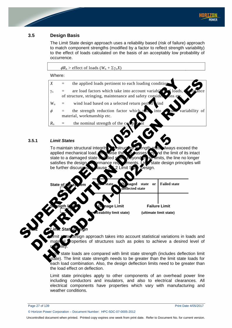
3.5.1 Limit States To maintain structural integrity, the structure strength must always exceed the applied mechanical load, otherwise the line passes beyond the limit of its intact state to a damaged state or failed state. Beyond these limits, the line no longer satisfies the design performance requirements. Limit state design principles will be further discussed in clause 3.5.2 Limit State Design.
State of the system
Strength limits Damage Limit Failure Limit (serviceability limit state) (ultimate limit state)
3.5.2 Limit State Design Limit state design approach takes into account statistical variations in loads and material properties of structures such as poles to achieve a desired level of reliability.
Limit state loads are compared with limit state strength (includes deflection limit state). The limit state strength needs to be greater than the limit state loads for each load combination. Also, the design deflection limits need to be greater than the load effect on deflection.
Limit state principles apply to other components of an overhead power line including conductors and insulators, and also to electrical clearances. All electrical components have properties which vary with manufacturing and weather conditions.
Intact state Damaged state or deflected state
Failed state
SUPERSEDED 04/0
5/201
7 BY
DISTRIB
UTION D
ESIGN R
ULES
HPC-9DJ-
01-0
002-
2015
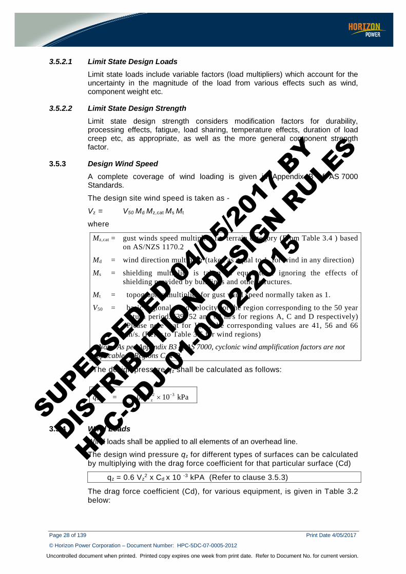
Page 28 of 139 Print Date 4/05/2017
© Horizon Power Corporation – Document Number: HPC-5DC-07-0005-2012
Uncontrolled document when printed. Printed copy expires one week from print date. Refer to Document No. for current version.
3.5.2.1 Limit State Design Loads Limit state loads include variable factors (load multipliers) which account for the uncertainty in the magnitude of the load from various effects such as wind, component weight etc.
3.5.2.2 Limit State Design Strength Limit state design strength considers modification factors for durability, processing effects, fatigue, load sharing, temperature effects, duration of load creep etc, as appropriate, as well as the more general component strength factor.
3.5.3 Design Wind Speed A complete coverage of wind loading is given in Appendix B of AS 7000 Standards.
The design site wind speed is taken as -
Vz = V50 Md Mz,cat Ms Mt
where
Mz,cat = gust winds speed multiplier for terrain category (From Table 3.4 ) based on AS/NZS 1170.2
Md = wind direction multiplier (taken as equal to 1, for wind in any direction)
Ms = shielding multiplier is taken as equal to 1 ignoring the effects of shielding provided by buildings and other structures.
Mt = topographic multiplier for gust wind speed normally taken as 1.
V50 = basic regional wind velocity for the region corresponding to the 50 year return period. (39, 52 and 60 m/s for regions A, C and D respectively) Please note that for V100 , the corresponding values are 41, 56 and 66 m/s. (Refer to Table 3.5 for wind regions)
Note: As per Appendix B3 of AS 7000, cyclonic wind amplification factors are not applicable to Regions C & D.
The design pressure qz shall be calculated as follows:
qz = 2 3z0.6 10 kPaV −×
3.5.4 Wind Loads Wind loads shall be applied to all elements of an overhead line.
The design wind pressure qz for different types of surfaces can be calculated by multiplying with the drag force coefficient for that particular surface (Cd)
qz = 0.6 Vz2 x Cd x 10 -3 kPA (Refer to clause 3.5.3)
The drag force coefficient (Cd), for various equipment, is given in Table 3.2 below:
SUPERSEDED 04/0
5/201
7 BY
DISTRIB
UTION D
ESIGN R
ULES
HPC-9DJ-
01-0
002-
2015
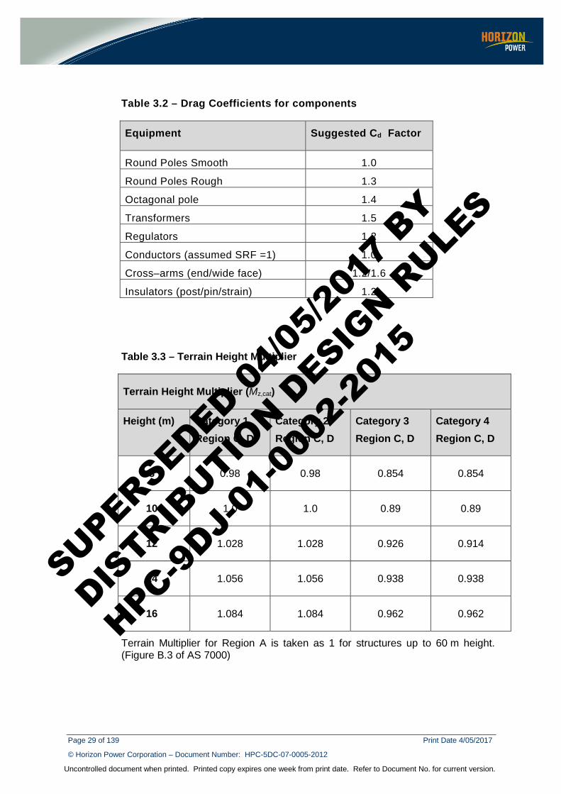
Page 29 of 139 Print Date 4/05/2017
© Horizon Power Corporation – Document Number: HPC-5DC-07-0005-2012
Uncontrolled document when printed. Printed copy expires one week from print date. Refer to Document No. for current version.
Table 3.2 – Drag Coefficients for components
Equipment Suggested Cd Factor
Round Poles Smooth 1.0
Round Poles Rough 1.3
Octagonal pole 1.4
Transformers 1.5
Regulators 1.2
Conductors (assumed SRF =1) 1.0
Cross–arms (end/wide face) 1.2/1.6
Insulators (post/pin/strain) 1.2
Table 3.3 – Terrain Height Multiplier
Terrain Height Multiplier (Mz,cat)
Height (m) Category 1 Region C, D
Category 2 Region C, D
Category 3 Region C, D
Category 4 Region C, D
8 0.98 0.98 0.854 0.854
10 1.0 1.0 0.89 0.89
12 1.028 1.028 0.926 0.914
14 1.056 1.056 0.938 0.938
16 1.084 1.084 0.962 0.962
Terrain Multiplier for Region A is taken as 1 for structures up to 60 m height. (Figure B.3 of AS 7000)
SUPERSEDED 04/0
5/201
7 BY
DISTRIB
UTION D
ESIGN R
ULES
HPC-9DJ-
01-0
002-
2015
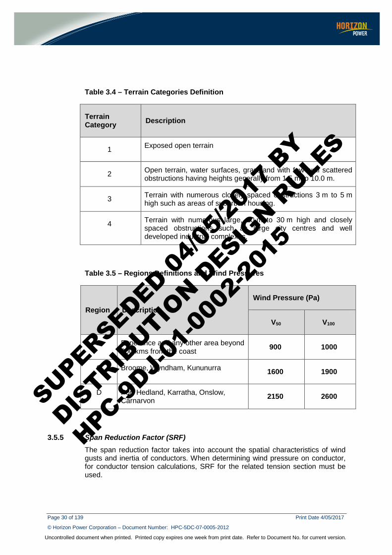
Page 30 of 139 Print Date 4/05/2017
© Horizon Power Corporation – Document Number: HPC-5DC-07-0005-2012
Uncontrolled document when printed. Printed copy expires one week from print date. Refer to Document No. for current version.
Table 3.4 – Terrain Categories Definition
Terrain Category Description
1 Exposed open terrain
2 Open terrain, water surfaces, grassland with few well scattered obstructions having heights generally from 1.5 m to 10.0 m.
3 Terrain with numerous closely spaced obstructions 3 m to 5 m high such as areas of suburban housing.
4 Terrain with numerous large, 10 m to 30 m high and closely spaced obstructions such as large city centres and well developed industrial complexes.
Table 3.5 – Regions Definitions and Wind Pressures
Region Description Wind Pressure (Pa)
V50 V100
A Esperance and any other area beyond 200 kms from the coast 900 1000
C Broome, Wyndham, Kununurra 1600 1900
D Port Hedland, Karratha, Onslow, Carnarvon 2150 2600
3.5.5 Span Reduction Factor (SRF) The span reduction factor takes into account the spatial characteristics of wind gusts and inertia of conductors. When determining wind pressure on conductor, for conductor tension calculations, SRF for the related tension section must be used.
SUPERSEDED 04/0
5/201
7 BY
DISTRIB
UTION D
ESIGN R
ULES
HPC-9DJ-
01-0
002-
2015
Page 31 of 139 Print Date 4/05/2017
© Horizon Power Corporation – Document Number: HPC-5DC-07-0005-2012
Uncontrolled document when printed. Printed copy expires one week from print date. Refer to Document No. for current version.
For Region A, SRF = 1, for spans up to 200 m and for spans > 200, calculate SRF using the formula:
SRF = 1.0 – (span length - 200)/1000 x 0.3125
For Regions C and D, calculate SRF using the formula:
SRF = 0.59 + 0.41 e (- span length/210)
3.5.6 Temperature
Ambient temperature for Region A is 40 °C (summer) and 15 °C (winter) and for Regions C & D 45 °C (summer) and 35 °C (winter).
Maximum conductor temperature must not exceed 75 °C, to ensure that electrical clearances are maintained.
3.6 Strength and Serviceability Limit States
3.6.1 Ultimate Strength Limit State Ultimate limit state is the maximum load carrying resistance of a structure or structural element. It is associated with collapse or other forms of structural failure due to excessive deformation, loss of stability, overturning, rupture or buckling.
3.6.2 Serviceability Limit State Serviceability limit state is the state beyond which specified service criteria for a structure or a structural element is no longer met. In this state, a structure and all its components mechanically function whilst maintaining prescribed electrical clearances.
3.6.3 Strength Reduction Factors
The strength reduction factor (φ) takes into account variability of material and workmanship for structural components used in overhead lines as well as some modification factors. Table 3.6 gives strength reduction factors applicable to different components of an overhead line.
Table 3.6 – Strength Reduction Factors (as per Table 6.2 of AS 7000)
Component of Overhead Line Limit State Strength Reduction Factor (φ)
Steel Poles and Cross arms Strength 0.9
Bolts, Nuts and Washers Strength 0.9
Untreated wood poles and cross-arms Strength 0.5
SUPERSEDED 04/0
5/201
7 BY
DISTRIB
UTION D
ESIGN R
ULES
HPC-9DJ-
01-0
002-
2015
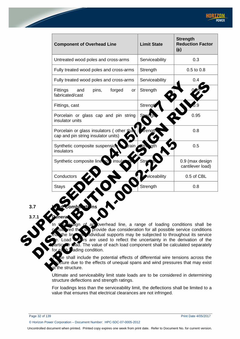
Page 32 of 139 Print Date 4/05/2017
© Horizon Power Corporation – Document Number: HPC-5DC-07-0005-2012
Uncontrolled document when printed. Printed copy expires one week from print date. Refer to Document No. for current version.
Component of Overhead Line Limit State Strength Reduction Factor (φ)
Untreated wood poles and cross-arms Serviceability 0.3
Fully treated wood poles and cross-arms Strength 0.5 to 0.8
Fully treated wood poles and cross-arms Serviceability 0.4
Fittings and pins, forged or fabricated/cast
Strength 0.95
Fittings, cast Strength 0.9
Porcelain or glass cap and pin string insulator units
Strength 0.95
Porcelain or glass insulators ( other than cap and pin string insulator units)
Strength 0.8
Synthetic composite suspension or strain insulators
Strength 0.5
Synthetic composite line post insulators Strength 0.9 (max design cantilever load)
Conductors Serviceability 0.5 of CBL
Stays Strength 0.8
3.7 Load Combinations
3.7.1 General In the design of an overhead line, a range of loading conditions shall be considered that will provide due consideration for all possible service conditions that the line and individual supports may be subjected to throughout its service life. Load factors are used to reflect the uncertainty in the derivation of the particular load. The value of each load component shall be calculated separately for each loading condition.
These shall include the potential effects of differential wire tensions across the structure due to the effects of unequal spans and wind pressures that may exist at the structure.
Ultimate and serviceability limit state loads are to be considered in determining structure deflections and strength ratings.
For loadings less than the serviceability limit, the deflections shall be limited to a value that ensures that electrical clearances are not infringed.
SUPERSEDED 04/0
5/201
7 BY
DISTRIB
UTION D
ESIGN R
ULES
HPC-9DJ-
01-0
002-
2015

Page 33 of 139 Print Date 4/05/2017
© Horizon Power Corporation – Document Number: HPC-5DC-07-0005-2012
Uncontrolled document when printed. Printed copy expires one week from print date. Refer to Document No. for current version.
3.7.1.1 Permanent Loads Self weight of structures, insulators, other fixed equipment and conductors resulting from adjacent spans act as permanent loads.
Vertical loads on poles foundations, cross-arms, insulators and fittings is the vertical force due to their own mass plus the mass of all ancillaries and attachments. (Gs).
Vertical loads of conductors/cables and attachments such as marker balls, spacers and dampers form the design weight span.(Gc)
3.7.2 Load Conditions and Load Factors The following load conditions and factors shall be used to determine the loading on structures:
Wn - wind load based on a selected wind period
Ft - load on structure due to intact horizontal component of conductor tension in the direction of the line for the appropriate wind load
Gc - Vertical load due to conductors
Gs - Vertical load due to cross-arms, insulators and fittings
3.7.2.1 Maximum Wind and Maximum Weight Determined by the equation: Wn +1.25 Ft + 1.1 Gs + 1.25 Gc (Table 7.3 of AS 7000)
3.7.2.2 Maximum Wind and Uplift Determined by the equation: Wn +1.25 Ft + 0.9 Gs + 1.25 Gc (Table 7.3 of AS 7000)
3.7.2.3 Everyday Condition (sustained load) Determined by the equation: 1.1 Ft + 1.1 Gs + 1.25 Gc (Table 7.3 of AS 7000)
3.7.2.4 Serviceability (deflection/damage limit) Determined by the equation: 1.0 Ft + 1.1 Gs + 1.1 Gc (Table 7.3 of AS 7000)
3.7.2.5 Failure Containment Load These loads are as a result of the failure of an adjacent structure. For the failure containment condition, supports shall be designed for the equivalent longitudinal loads resulting from conductors on the structure being broken with a minimum coincident wind pressure of 0.25 times the ultimate design wind pressure (Wn). The unbalance tension (Fb) resulting from these broken conductors is the residual static load (RSL) in the aerial phase conductors after severance of a conductor, or the collapse of a conductor support system. For aerial conductors supported by suspension insulator strings, an RSL factor of 0.7 must be used, otherwise 0.8 is used.
The unbroken conductors will be subject to the “Intact Conductor Tensions (Ft)”.
SUPERSEDED 04/0
5/201
7 BY
DISTRIB
UTION D
ESIGN R
ULES
HPC-9DJ-
01-0
002-
2015
Page 34 of 139 Print Date 4/05/2017
© Horizon Power Corporation – Document Number: HPC-5DC-07-0005-2012
Uncontrolled document when printed. Printed copy expires one week from print date. Refer to Document No. for current version.
Fb and Ft tensions for conductors are based on the temperature corresponding to the everyday load condition with a minimum nominal wind pressure of 0.25 times the ultimate design wind pressure.
Accordingly, total load on a structure is:
0.25Wn +1.25 Ft + 1.1 Gs + 1.25 Gc + 1.25 Fb
SUPERSEDED 04/0
5/201
7 BY
DISTRIB
UTION D
ESIGN R
ULES
HPC-9DJ-
01-0
002-
2015
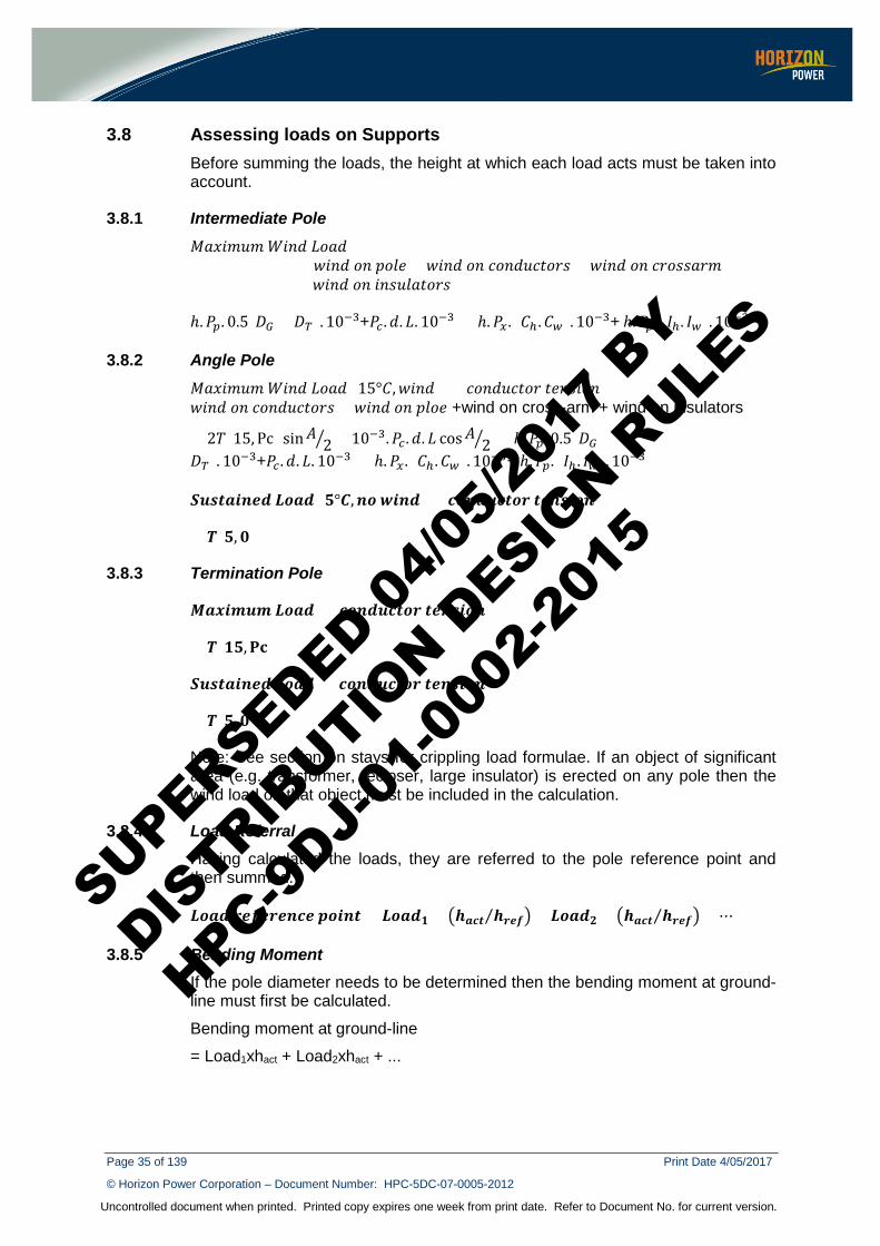
Page 35 of 139 Print Date 4/05/2017
© Horizon Power Corporation – Document Number: HPC-5DC-07-0005-2012
Uncontrolled document when printed. Printed copy expires one week from print date. Refer to Document No. for current version.
3.8 Assessing loads on Supports Before summing the loads, the height at which each load acts must be taken into account.
3.8.1 Intermediate Pole 𝑀𝑀𝑀𝑀𝑀𝑀𝑀𝑀𝑀𝑀𝑀𝑀𝑀𝑀 𝑊𝑊𝑀𝑀𝑊𝑊𝑊𝑊 𝐿𝐿𝐿𝐿𝑀𝑀𝑊𝑊
= 𝑤𝑤𝑀𝑀𝑊𝑊𝑊𝑊 𝐿𝐿𝑊𝑊 𝑝𝑝𝐿𝐿𝑝𝑝𝑝𝑝 + 𝑤𝑤𝑀𝑀𝑊𝑊𝑊𝑊 𝐿𝐿𝑊𝑊 𝑐𝑐𝐿𝐿𝑊𝑊𝑊𝑊𝑀𝑀𝑐𝑐𝑐𝑐𝐿𝐿𝑐𝑐𝑐𝑐 + 𝑤𝑤𝑀𝑀𝑊𝑊𝑊𝑊 𝐿𝐿𝑊𝑊 𝑐𝑐𝑐𝑐𝐿𝐿𝑐𝑐𝑐𝑐𝑀𝑀𝑐𝑐𝑀𝑀 + 𝑤𝑤𝑀𝑀𝑊𝑊𝑊𝑊 𝐿𝐿𝑊𝑊 𝑀𝑀𝑊𝑊𝑐𝑐𝑀𝑀𝑝𝑝𝑀𝑀𝑐𝑐𝐿𝐿𝑐𝑐𝑐𝑐
ℎ.𝑃𝑃𝑝𝑝. 0.5(𝐷𝐷𝐺𝐺 + 𝐷𝐷𝑇𝑇). 10−3+𝑃𝑃𝑐𝑐 .𝑊𝑊. 𝐿𝐿. 10−3 + ℎ.𝑃𝑃𝑥𝑥 . (𝐶𝐶ℎ .𝐶𝐶𝑤𝑤). 10−3+ ℎ.𝑃𝑃𝑝𝑝. (𝐼𝐼ℎ. 𝐼𝐼𝑤𝑤). 10−3
3.8.2 Angle Pole 𝑀𝑀𝑀𝑀𝑀𝑀𝑀𝑀𝑀𝑀𝑀𝑀𝑀𝑀 𝑊𝑊𝑀𝑀𝑊𝑊𝑊𝑊 𝐿𝐿𝐿𝐿𝑀𝑀𝑊𝑊 (15°𝐶𝐶,𝑤𝑤𝑀𝑀𝑊𝑊𝑊𝑊) = 𝑐𝑐𝐿𝐿𝑊𝑊𝑊𝑊𝑀𝑀𝑐𝑐𝑐𝑐𝐿𝐿𝑐𝑐 𝑐𝑐𝑝𝑝𝑊𝑊𝑐𝑐𝑀𝑀𝐿𝐿𝑊𝑊 +𝑤𝑤𝑀𝑀𝑊𝑊𝑊𝑊 𝐿𝐿𝑊𝑊 𝑐𝑐𝐿𝐿𝑊𝑊𝑊𝑊𝑀𝑀𝑐𝑐𝑐𝑐𝐿𝐿𝑐𝑐𝑐𝑐 + 𝑤𝑤𝑀𝑀𝑊𝑊𝑊𝑊 𝐿𝐿𝑊𝑊 𝑝𝑝𝑝𝑝𝐿𝐿𝑝𝑝 +wind on cross-arm + wind on insulators
= 2𝑇𝑇(15, Pc) sin𝐴𝐴 2 + 10−3.𝑃𝑃𝑐𝑐 .𝑊𝑊. 𝐿𝐿 cos𝐴𝐴 2 + ℎ.𝑃𝑃𝑝𝑝. 0.5(𝐷𝐷𝐺𝐺 +𝐷𝐷𝑇𝑇). 10−3+𝑃𝑃𝑐𝑐 .𝑊𝑊. 𝐿𝐿. 10−3 + ℎ.𝑃𝑃𝑥𝑥 . (𝐶𝐶ℎ .𝐶𝐶𝑤𝑤). 10−3+ ℎ.𝑃𝑃𝑝𝑝. (𝐼𝐼ℎ . 𝐼𝐼𝑤𝑤). 10−3
𝑺𝑺𝑺𝑺𝑺𝑺𝑺𝑺𝑺𝑺𝑺𝑺𝑺𝑺𝑺𝑺𝑺𝑺 𝑳𝑳𝑳𝑳𝑺𝑺𝑺𝑺 (𝟓𝟓°𝑪𝑪,𝑺𝑺𝑳𝑳 𝒘𝒘𝑺𝑺𝑺𝑺𝑺𝑺) = 𝒄𝒄𝑳𝑳𝑺𝑺𝑺𝑺𝑺𝑺𝒄𝒄𝑺𝑺𝑳𝑳𝒄𝒄 𝑺𝑺𝑺𝑺𝑺𝑺𝑺𝑺𝑺𝑺𝑳𝑳𝑺𝑺
= 𝑻𝑻(𝟓𝟓,𝟎𝟎)
3.8.3 Termination Pole
𝑴𝑴𝑺𝑺𝑴𝑴𝑺𝑺𝑴𝑴𝑺𝑺𝑴𝑴 𝑳𝑳𝑳𝑳𝑺𝑺𝑺𝑺 = 𝒄𝒄𝑳𝑳𝑺𝑺𝑺𝑺𝑺𝑺𝒄𝒄𝑺𝑺𝑳𝑳𝒄𝒄 𝑺𝑺𝑺𝑺𝑺𝑺𝑺𝑺𝑺𝑺𝑳𝑳𝑺𝑺
= 𝑻𝑻(𝟏𝟏𝟓𝟓,𝐏𝐏𝐏𝐏)
𝑺𝑺𝑺𝑺𝑺𝑺𝑺𝑺𝑺𝑺𝑺𝑺𝑺𝑺𝑺𝑺𝑺𝑺 𝑳𝑳𝑳𝑳𝑺𝑺𝑺𝑺 = 𝒄𝒄𝑳𝑳𝑺𝑺𝑺𝑺𝑺𝑺𝒄𝒄𝑺𝑺𝑳𝑳𝒄𝒄 𝑺𝑺𝑺𝑺𝑺𝑺𝑺𝑺𝑺𝑺𝑳𝑳𝑺𝑺
= 𝑻𝑻(𝟓𝟓,𝟎𝟎)
Note: See section on stays for crippling load formulae. If an object of significant area (e.g. transformer, recloser, large insulator) is erected on any pole then the wind load on that object must be included in the calculation.
3.8.4 Load Referral Having calculated the loads, they are referred to the pole reference point and then summed.
𝑳𝑳𝑳𝑳𝑺𝑺𝑺𝑺 𝒄𝒄𝑺𝑺𝒓𝒓𝑺𝑺𝒄𝒄𝑺𝑺𝑺𝑺𝒄𝒄𝑺𝑺 𝒑𝒑𝑳𝑳𝑺𝑺𝑺𝑺𝑺𝑺 = 𝑳𝑳𝑳𝑳𝑺𝑺𝑺𝑺𝟏𝟏 × 𝒉𝒉𝑺𝑺𝒄𝒄𝑺𝑺 𝒉𝒉𝒄𝒄𝑺𝑺𝒓𝒓⁄ + 𝑳𝑳𝑳𝑳𝑺𝑺𝑺𝑺𝟐𝟐 × 𝒉𝒉𝑺𝑺𝒄𝒄𝑺𝑺 𝒉𝒉𝒄𝒄𝑺𝑺𝒓𝒓⁄ + ⋯
3.8.5 Bending Moment If the pole diameter needs to be determined then the bending moment at ground-line must first be calculated.
Bending moment at ground-line
= Load1xhact + Load2xhact + ...
SUPERSEDED 04/0
5/201
7 BY
DISTRIB
UTION D
ESIGN R
ULES
HPC-9DJ-
01-0
002-
2015
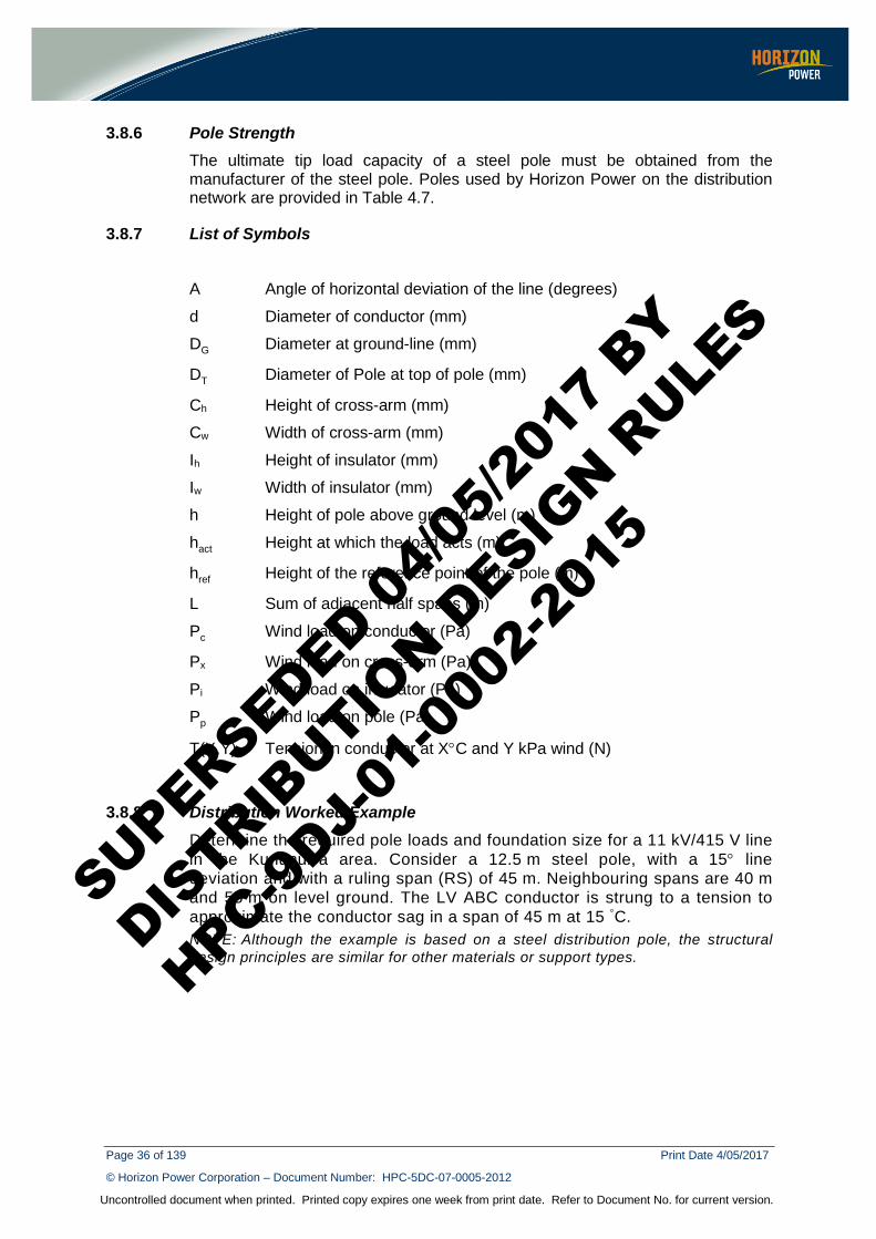
Page 36 of 139 Print Date 4/05/2017
© Horizon Power Corporation – Document Number: HPC-5DC-07-0005-2012
Uncontrolled document when printed. Printed copy expires one week from print date. Refer to Document No. for current version.
3.8.6 Pole Strength The ultimate tip load capacity of a steel pole must be obtained from the manufacturer of the steel pole. Poles used by Horizon Power on the distribution network are provided in Table 4.7.
3.8.7 List of Symbols
A Angle of horizontal deviation of the line (degrees)
d Diameter of conductor (mm)
DG Diameter at ground-line (mm)
DT Diameter of Pole at top of pole (mm)
Ch Height of cross-arm (mm)
Cw Width of cross-arm (mm)
Ih Height of insulator (mm)
Iw Width of insulator (mm)
h Height of pole above ground level (m)
hact Height at which the load acts (m)
href Height of the reference point of the pole (m)
L Sum of adjacent half spans (m)
Pc Wind load on conductor (Pa)
Px Wind load on cross-arm (Pa)
Pi Wind load on insulator (Pa)
Pp Wind load on pole (Pa)
T(X,Y) Tension in conductor at X°C and Y kPa wind (N)
3.8.8 Distribution Worked Example Determine the required pole loads and foundation size for a 11 kV/415 V line in the Kununurra area. Consider a 12.5 m steel pole, with a 15° line deviation and with a ruling span (RS) of 45 m. Neighbouring spans are 40 m and 55 m on level ground. The LV ABC conductor is strung to a tension to approximate the conductor sag in a span of 45 m at 15 °C. NOTE: Although the example is based on a steel distribution pole, the structural design principles are similar for other materials or support types.
SUPERSEDED 04/0
5/201
7 BY
DISTRIB
UTION D
ESIGN R
ULES
HPC-9DJ-
01-0
002-
2015

Page 37 of 139 Print Date 4/05/2017
© Horizon Power Corporation – Document Number: HPC-5DC-07-0005-2012
Uncontrolled document when printed. Printed copy expires one week from print date. Refer to Document No. for current version.
DESIGN DATA 11 kV Conductor type: 19/3.75 AAC (Pluto) to AS 1531 strung at 5% of CBL at 15°C.
Conductor Dia Mass Area Mod of E Exp Coef CBL
(mm) (kg/m) (mm2) (MPa) (/deg C) (kN)
Pluto 18.8 0.576 209.8 65000 0.000023 31.9
11 kV Conductor positions: Conductor 1: 1.2 m left, 10.2 m above ground
Conductor 2: above top of pole, 10.6 m above ground
Conductor 3: 1.2 m right, 10.2 m above ground
415 V Cable type: 4 × 95 mm2 LV Aerial Bundled Cable (ABC) to AS/NZS 3560 and strung at 7% of CBL at 15°C.
Conductor Dia Mass Area Mod of E Exp Coef CBL
(mm) (kg/m) (mm2) (MPa) (/deg C) (kN)
4/95 ABC 38.4 1.35 380 56000 0.000023 53.2
415 V Cable position: 0.225 m left, 8.7 m above ground
Pole details: Manufactured to Horizon Power Technical Specification for Fabricated Poles on the Distribution Network (Initially assume a 16 kN/12.5 m steel tubular Pole)
Top diameter 125 mm
Ground line diameter 395 mm
Height above ground 10.2 m (i.e. depth in ground 2.3 m)
Cross-arm size: 100 by 150 mm
11 kV insulators are ALP 11/275
The soil conditions are specified in three layers: 0-0.5 m of loose gravel with sand, 0.5-1.0 m of firm cohesive soil and 1.0 m or more of very stiff cohesive soil.
CALCULATIONS
LV Bracket - ABC
8700
400
102
200
1200 1200
SUPERSEDED 04/0
5/201
7 BY
DISTRIB
UTION D
ESIGN R
ULES
HPC-9DJ-
01-0
002-
2015
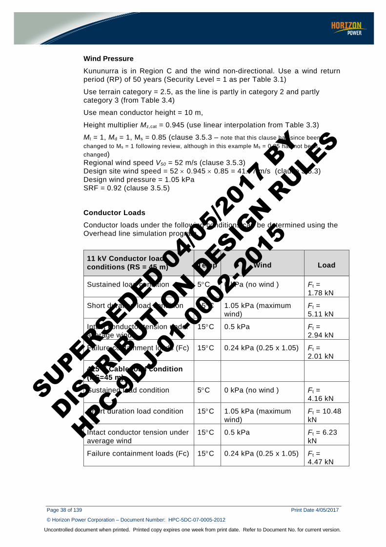
Page 38 of 139 Print Date 4/05/2017
© Horizon Power Corporation – Document Number: HPC-5DC-07-0005-2012
Uncontrolled document when printed. Printed copy expires one week from print date. Refer to Document No. for current version.
Wind Pressure Kununurra is in Region C and the wind non-directional. Use a wind return period (RP) of 50 years (Security Level = 1 as per Table 3.1)
Use terrain category = 2.5, as the line is partly in category 2 and partly category 3 (from Table 3.4)
Use mean conductor height = 10 m,
Height multiplier Mz,cat = 0.945 (use linear interpolation from Table 3.3)
Mt = 1, Md = 1, Ms = 0.85 (clause 3.5.3 – note that this clause has since been changed to Ms = 1 following review, although in this example Ms = 0.85 has not been changed) Regional wind speed V50 = 52 m/s (clause 3.5.3) Design site wind speed = 52 × 0.945 × 0.85 = 41.77 m/s (clause 3.5.3) Design wind pressure = 1.05 kPa SRF = 0.92 (clause 3.5.5)
Conductor Loads Conductor loads under the following conditions can be determined using the Overhead line simulation program.
11 kV Conductor load conditions (RS = 45 m) Temp Wind Load
Sustained load condition 5°C 0 kPa (no wind ) Ft = 1.78 kN
Short duration load condition 15°C 1.05 kPa (maximum wind)
Ft = 5.11 kN
Intact conductor tension under average wind
15°C 0.5 kPa Ft = 2.94 kN
Failure containment loads (Fc) 15°C 0.24 kPa (0.25 x 1.05) Ft = 2.01 kN
415 V Cable load condition (RS=45 m)
Sustained load condition 5°C 0 kPa (no wind ) Ft = 4.16 kN
Short duration load condition 15°C 1.05 kPa (maximum wind)
Ft = 10.48 kN
Intact conductor tension under average wind
15°C 0.5 kPa Ft = 6.23 kN
Failure containment loads (Fc) 15°C 0.24 kPa (0.25 x 1.05) Ft = 4.47 kN
SUPERSEDED 04/0
5/201
7 BY
DISTRIB
UTION D
ESIGN R
ULES
HPC-9DJ-
01-0
002-
2015
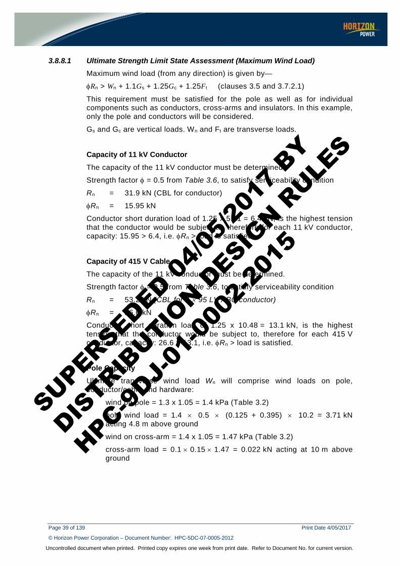
Page 39 of 139 Print Date 4/05/2017
© Horizon Power Corporation – Document Number: HPC-5DC-07-0005-2012
Uncontrolled document when printed. Printed copy expires one week from print date. Refer to Document No. for current version.
3.8.8.1 Ultimate Strength Limit State Assessment (Maximum Wind Load) Maximum wind load (from any direction) is given by—
φRn > Wn + 1.1Gs + 1.25Gc + 1.25Ft (clauses 3.5 and 3.7.2.1)
This requirement must be satisfied for the pole as well as for individual components such as conductors, cross-arms and insulators. In this example, only the pole and conductors will be considered.
Gs and Gc are vertical loads. Wn and Ft are transverse loads.
Capacity of 11 kV Conductor The capacity of the 11 kV conductor must be determined.
Strength factor φ = 0.5 from Table 3.6, to satisfy serviceability condition
Rn = 31.9 kN (CBL for conductor)
φRn = 15.95 kN
Conductor short duration load of 1.25 x 5.11 = 6.4 kN, is the highest tension that the conductor would be subject to, therefore for each 11 kV conductor, capacity: 15.95 > 6.4, i.e. φRn > load is satisfied.
Capacity of 415 V Cable The capacity of the 11 kV conductor must be determined.
Strength factor φ = 0.5 from Table 3.6, to satisfy serviceability condition
Rn = 53.2 kN (CBL for 4 × 95 LV ABC conductor)
φRn = 26.6 kN
Conductor short duration load of 1.25 x 10.48 = 13.1 kN, is the highest tension that the conductor would be subject to, therefore for each 415 V conductor, capacity: 26.6 > 13.1, i.e. φRn > load is satisfied.
Pole Capacity Ultimate transverse wind load Wn will comprise wind loads on pole, conductor/cable and hardware:
wind on pole = 1.3 x 1.05 = 1.4 kPa (Table 3.2)
pole wind load = 1.4 × 0.5 × (0.125 + 0.395) × 10.2 = 3.71 kN acting 4.8 m above ground
wind on cross-arm = 1.4 x 1.05 = 1.47 kPa (Table 3.2)
cross-arm load = 0.1 × 0.15 × 1.47 = 0.022 kN acting at 10 m above ground
SUPERSEDED 04/0
5/201
7 BY
DISTRIB
UTION D
ESIGN R
ULES
HPC-9DJ-
01-0
002-
2015
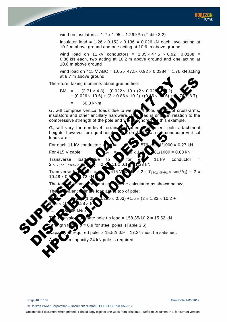
Page 40 of 139 Print Date 4/05/2017
© Horizon Power Corporation – Document Number: HPC-5DC-07-0005-2012
Uncontrolled document when printed. Printed copy expires one week from print date. Refer to Document No. for current version.
wind on insulators = 1.2 x 1.05 = 1.26 kPa (Table 3.2)
insulator load = 1.26 × 0.152 × 0.136 = 0.026 kN each, two acting at 10.2 m above ground and one acting at 10.6 m above ground
wind load on 11 kV conductors = 1.05 × 47.5 × 0.92 × 0.0188 = 0.86 kN each, two acting at 10.2 m above ground and one acting at 10.6 m above ground
wind load on 415 V ABC = 1.05 × 47.5× 0.92 × 0.0384 = 1.76 kN acting at 8.7 m above ground
Therefore, taking moments about ground line:
BM = (3.71 × 4.8) + (0.022 × 10 + (2 × 0.026 × 10.2) + (0.026 × 10.6) + (2 × 0.86 × 10.2) +(0.86 × 10.6) + (1.76 × 8.7)
= 60.8 kNm
Gs will comprise vertical loads due to weight of pole, weight of cross-arms, insulators and other ancillary hardware. This load is small in relation to the compressive strength of the pole and will be ignored for this example.
Gc will vary for non-level terrain and unequal adjacent pole attachment heights, however for equal height poles on flat terrain the conductor vertical loads are—
For each 11 kV conductor: Gc = 47.5 x 0.576 x 9.81/1000 = 0.27 kN
For 415 V cable: Gc = 47.5 x 1.35 x 9.81/1000 = 0.63 kN
Transverse load due to Ft for each 11 kV conductor = 2 × T15C,1.05kPa × sin(15/2) = 2 x 5.11 x 0.13 = 1.33 kN
Transverse load due to Ft for 415 V cable = 2 × T15C,1.05kPa × sin(15/2) = 2 x 10.48 x 0.13 = 2.72 kN
The total pole base moment can now be calculated as shown below:
The equivalent ultimate load at the top of pole:
BMtot = 60.8 + (1.25 × 0.225 × 0.63) +1.5 × (2 × 1.33 × 10.2 + 1.76 × 10.6 + 3.58 × 8.7)
= 158.35 kNm
The equivalent ultimate pole tip load = 158.35/10.2 = 15.52 kN
Strength factor φ = 0.9 for steel poles. (Table 3.6)
Capacity of required pole > 15.52/ 0.9 = 17.24 must be satisfied.
A minimum capacity 24 kN pole is required.
SUPERSEDED 04/0
5/201
7 BY
DISTRIB
UTION D
ESIGN R
ULES
HPC-9DJ-
01-0
002-
2015
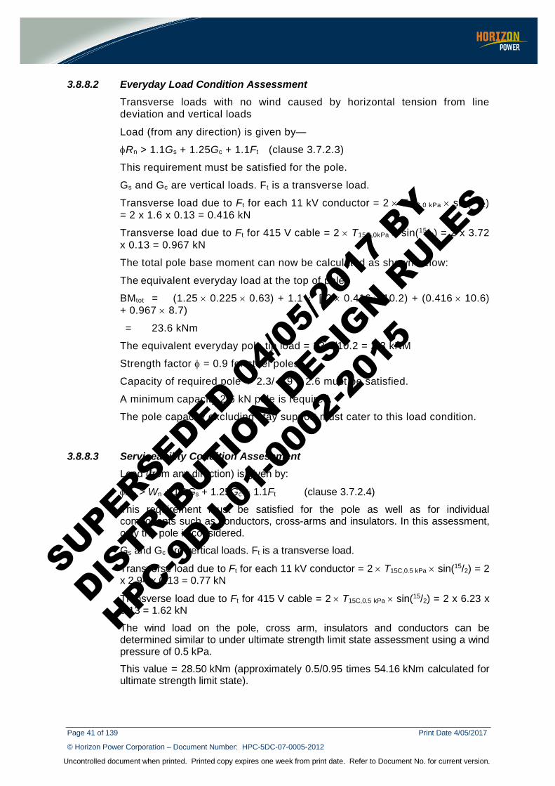
Page 41 of 139 Print Date 4/05/2017
© Horizon Power Corporation – Document Number: HPC-5DC-07-0005-2012
Uncontrolled document when printed. Printed copy expires one week from print date. Refer to Document No. for current version.
3.8.8.2 Everyday Load Condition Assessment Transverse loads with no wind caused by horizontal tension from line deviation and vertical loads
Load (from any direction) is given by—
φRn > 1.1Gs + 1.25Gc + 1.1Ft (clause 3.7.2.3)
This requirement must be satisfied for the pole.
Gs and Gc are vertical loads. Ft is a transverse load.
Transverse load due to Ft for each 11 kV conductor = 2 × T15C,0 kPa × sin(15/2) = 2 x 1.6 x 0.13 = 0.416 kN
Transverse load due to Ft for 415 V cable = 2 × T15C,0kPa × sin(15/2) = 2 x 3.72 x 0.13 = 0.967 kN
The total pole base moment can now be calculated as shown below:
The equivalent everyday load at the top of pole:
BMtot = (1.25 × 0.225 × 0.63) + 1.1 × [(2 × 0.416 × 10.2) + (0.416 × 10.6) + 0.967 × 8.7)
= 23.6 kNm
The equivalent everyday pole tip load = 23.6/10.2 = 2.3 kNM
Strength factor φ = 0.9 for steel poles.
Capacity of required pole > 2.3/ 0.9 = 2.6 must be satisfied.
A minimum capacity 2.6 kN pole is required.
The pole capacity excluding stay support must cater to this load condition.
3.8.8.3 Serviceability Condition Assessment Load (from any direction) is given by:
φRn > Wn + 1.1Gs + 1.25Gc + 1.1Ft (clause 3.7.2.4)
This requirement must be satisfied for the pole as well as for individual components such as conductors, cross-arms and insulators. In this assessment, only the pole is considered.
Gs and Gc are vertical loads. Ft is a transverse load.
Transverse load due to Ft for each 11 kV conductor = 2 × T15C,0.5 kPa × sin(15/2) = 2 x 2.94 x 0.13 = 0.77 kN
Transverse load due to Ft for 415 V cable = 2 × T15C,0.5 kPa × sin(15/2) = 2 x 6.23 x 0.13 = 1.62 kN
The wind load on the pole, cross arm, insulators and conductors can be determined similar to under ultimate strength limit state assessment using a wind pressure of 0.5 kPa.
This value = 28.50 kNm (approximately 0.5/0.95 times 54.16 kNm calculated for ultimate strength limit state).
SUPERSEDED 04/0
5/201
7 BY
DISTRIB
UTION D
ESIGN R
ULES
HPC-9DJ-
01-0
002-
2015
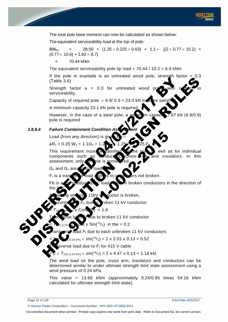
Page 42 of 139 Print Date 4/05/2017
© Horizon Power Corporation – Document Number: HPC-5DC-07-0005-2012
Uncontrolled document when printed. Printed copy expires one week from print date. Refer to Document No. for current version.
The total pole base moment can now be calculated as shown below:
The equivalent serviceability load at the top of pole:
BMtot = 28.50 + (1.25 × 0.225 × 0.63) + 1.1 × [(2 × 0.77 × 10.2) + (0.77 × 10.6) + 1.62 × 8.7)
= 70.44 kNm
The equivalent serviceability pole tip load = 70.44 / 10.2 = 6.9 kNm
If the pole in example is an untreated wood pole, strength factor = 0.3 (Table 3.6)
Strength factor φ = 0.3 for untreated wood poles with respect to serviceability.
Capacity of required pole > 6.9/ 0.3 = 23.0 kN must be satisfied.
A minimum capacity 23.1 kN pole is required.
However, in the case of a steel pole, a minimum capacity 7.67 kN (6.9/0.9) pole is required
3.8.8.4 Failure Containment Condition Assessment Load (from any direction) is given by—
φRn > 0.25 Wn + 1.1Gs + 1.25Gc + 1.25 Ft + 1.25 Fb
This requirement must be satisfied for the pole as well as for individual components such as conductors, cross-arms and insulators. In this assessment, only the pole is considered.
Gs and Gc are vertical loads.
Ft is a transverse load applied to conductors not broken.
Fb is a the residual static load (RSL) in broken conductors in the direction of the line.
Assuming one side 11kV conductor is broken,
Horizontal load Fb due to broken 11 kV conductor
= T15C,0.24 kPa x Cos(15/2) = 1.6
Transverse load Fb due to broken 11 kV conductor
= T15C,0.24 kPa x 0.8 x Sin(15/2) in the = 0.2
Transverse load Ft due to each unbroken 11 kV conductors
= 2 x T15C,0.24 kPa × sin(15/2) = 2 x 2.01 x 0.13 = 0.52
Transverse load due to Ft for 415 V cable
= 2 × T15C,0.24 kPa × sin(15/2) = 2 x 4.47 x 0.13 = 1.16 kN.
The wind load on the pole, cross arm, insulators and conductors can be determined similar to under ultimate strength limit state assessment using a wind pressure of 0.24 kPa.
This value = 13.68 kNm (approximately 0.24/0.95 times 54.16 kNm calculated for ultimate strength limit state).
SUPERSEDED 04/0
5/201
7 BY
DISTRIB
UTION D
ESIGN R
ULES
HPC-9DJ-
01-0
002-
2015
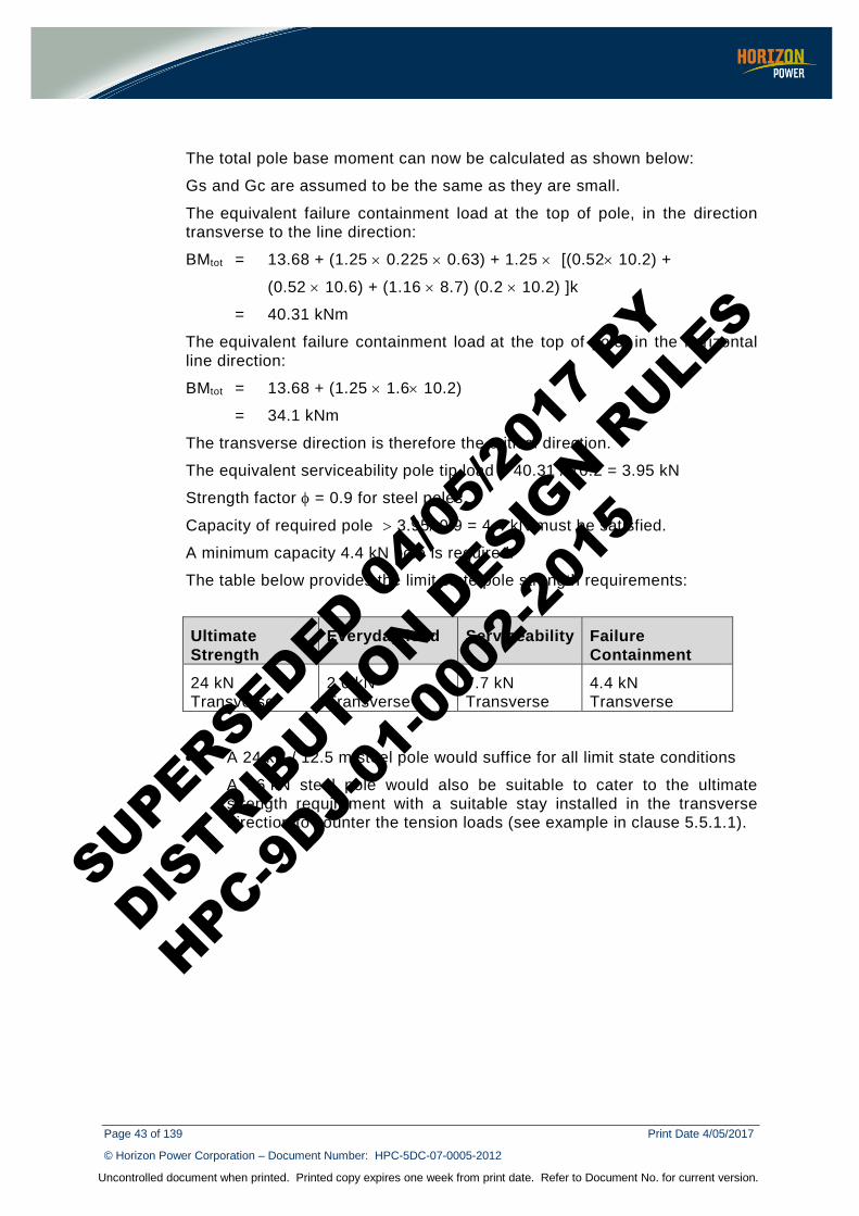
Page 43 of 139 Print Date 4/05/2017
© Horizon Power Corporation – Document Number: HPC-5DC-07-0005-2012
Uncontrolled document when printed. Printed copy expires one week from print date. Refer to Document No. for current version.
The total pole base moment can now be calculated as shown below:
Gs and Gc are assumed to be the same as they are small.
The equivalent failure containment load at the top of pole, in the direction transverse to the line direction:
BMtot = 13.68 + (1.25 × 0.225 × 0.63) + 1.25 × [(0.52× 10.2) +
(0.52 × 10.6) + (1.16 × 8.7) (0.2 × 10.2) ]k
= 40.31 kNm
The equivalent failure containment load at the top of pole, in the horizontal line direction:
BMtot = 13.68 + (1.25 × 1.6× 10.2)
= 34.1 kNm
The transverse direction is therefore the critical direction.
The equivalent serviceability pole tip load = 40.31 / 10.2 = 3.95 kN
Strength factor φ = 0.9 for steel poles.
Capacity of required pole > 3.95/ 0.9 = 4.4 kN must be satisfied.
A minimum capacity 4.4 kN pole is required.
The table below provides the limit state pole strength requirements:
Ultimate Strength
Everyday load Serviceability Failure Containment
24 kN Transverse
2.6 kN Transverse
7.7 kN Transverse
4.4 kN Transverse
• A 24 kN / 12.5 m steel pole would suffice for all limit state conditions
• A 16 kN steel pole would also be suitable to cater to the ultimate strength requirement with a suitable stay installed in the transverse direction to counter the tension loads (see example in clause 5.5.1.1).
SUPERSEDED 0
4/05/2
017
BY
DISTRIB
UTION D
ESIGN R
ULES
HPC-9DJ-
01-0
002-
2015
Page 44 of 139 Print Date 4/05/2017
© Horizon Power Corporation – Document Number: HPC-5DC-07-0005-2012
Uncontrolled document when printed. Printed copy expires one week from print date. Refer to Document No. for current version.
4 SUPPORT DESIGN
4.1 Guidelines a) The projected area of cylindrical surfaces shall be taken at right angles to
the wind direction, and no allowance should be made for the shielding of one conductor by another, but the full area of members of both the windward and leeward sides of the structure shall be taken as being exposed to wind pressure.
b) Intermediate (in line) poles must consider wind loads on the conductors, pole and all attachments.
c) Angle poles shall consider wind loads on the pole and all fittings plus tension loads in the conductors. When designing for the maximum wind load condition the tension used shall be the tension which is developed in the conductors under maximum wind load conditions. Also, the pole shall be designed to withstand sustained tension loads in the conductors under everyday (still air) conditions.
d) Terminal poles shall consider:
I. in the line direction - the maximum wind loads and sustained load in the conductors; and
II. in the transverse direction - the maximum wind loads on the conductors, poles, stay wire and all attachments.
e) If the design load calculated for ultimate strength conditions exceeds the available pole capacity, then a stay shall be installed to counter tension loads.
4.2 Pole Selection A range of pole sizes is available for use. Each has a specific maximum load rating as given in Table 4.7. The rating refers to the maximum load that can be applied at a point 300 mm below the crown of the pole.
Once the total load of the conductor plus equipment (refer to load combinations in section 3.7) is known then a suitable size pole can be chosen, with a load rating equal to or in excess of the total load.
Care must be taken to include anticipated (future) additions or modifications that maybe carried out to the pole structure, to ensure that the correct load rating is selected.
When selecting a pole of the required size (rating) the following steps must be taken:
1) Determine:
a) type of structure to be erected
b) conductor type and size to be used
c) the bay length
d) all associated fittings to be mounted on the pole
e) wind speed in region of installation
SUPERSEDED 04/0
5/201
7 BY
DISTRIB
UTION D
ESIGN R
ULES
HPC-9DJ-
01-0
002-
2015
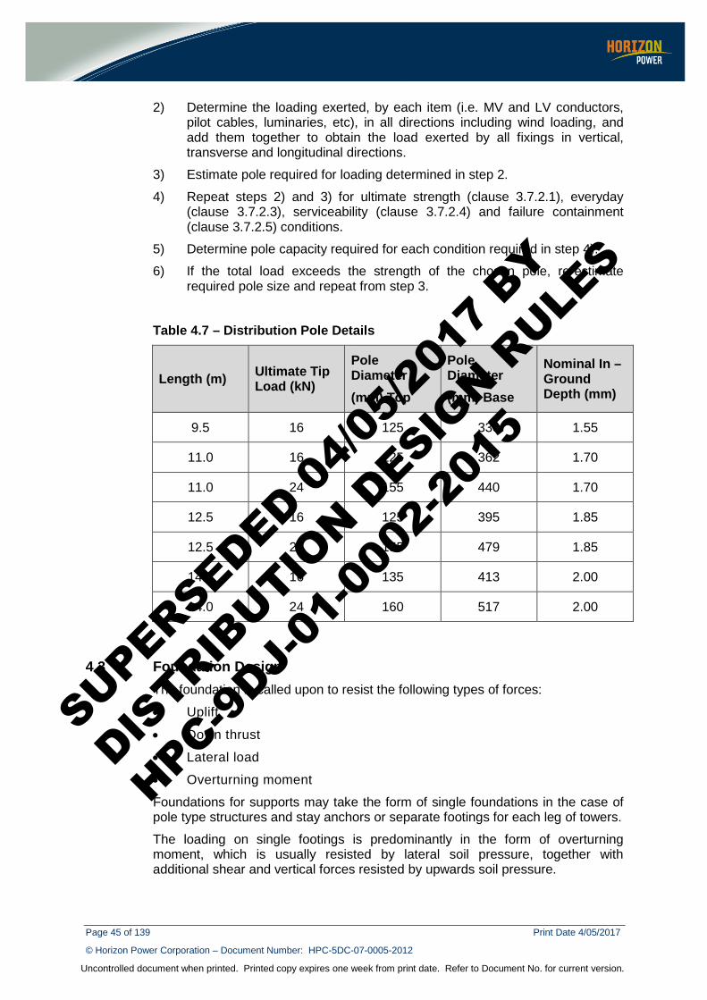
Page 45 of 139 Print Date 4/05/2017
© Horizon Power Corporation – Document Number: HPC-5DC-07-0005-2012
Uncontrolled document when printed. Printed copy expires one week from print date. Refer to Document No. for current version.
2) Determine the loading exerted, by each item (i.e. MV and LV conductors, pilot cables, luminaries, etc), in all directions including wind loading, and add them together to obtain the load exerted by all fixings in vertical, transverse and longitudinal directions.
3) Estimate pole required for loading determined in step 2.
4) Repeat steps 2) and 3) for ultimate strength (clause 3.7.2.1), everyday (clause 3.7.2.3), serviceability (clause 3.7.2.4) and failure containment (clause 3.7.2.5) conditions.
5) Determine pole capacity required for each condition required in step 4).
6) If the total load exceeds the strength of the chosen pole, re-estimate required pole size and repeat from step 3.
Table 4.7 – Distribution Pole Details
Length (m) Ultimate Tip Load (kN)
Pole Diameter (mm) Top
Pole Diameter (mm) Base
Nominal In –Ground Depth (mm)
9.5 16 125 330 1.55
11.0 16 125 362 1.70
11.0 24 155 440 1.70
12.5 16 125 395 1.85
12.5 24 155 479 1.85
14.0 16 135 413 2.00
14.0 24 160 517 2.00
4.3 Foundation Design The foundation is called upon to resist the following types of forces:
• Uplift
• Down thrust
• Lateral load
• Overturning moment
Foundations for supports may take the form of single foundations in the case of pole type structures and stay anchors or separate footings for each leg of towers.
The loading on single footings is predominantly in the form of overturning moment, which is usually resisted by lateral soil pressure, together with additional shear and vertical forces resisted by upwards soil pressure.
SUPERSEDED 04/0
5/201
7 BY
DISTRIB
UTION D
ESIGN R
ULES
HPC-9DJ-
01-0
002-
2015
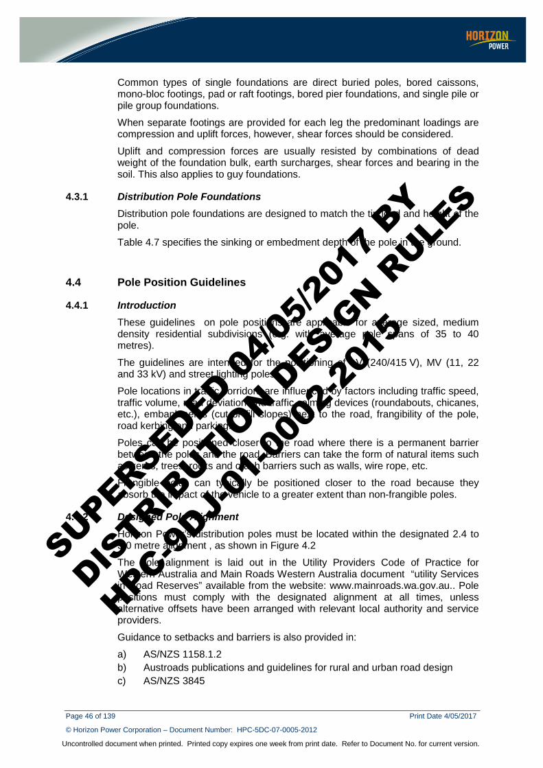
Page 46 of 139 Print Date 4/05/2017
© Horizon Power Corporation – Document Number: HPC-5DC-07-0005-2012
Uncontrolled document when printed. Printed copy expires one week from print date. Refer to Document No. for current version.
Common types of single foundations are direct buried poles, bored caissons, mono-bloc footings, pad or raft footings, bored pier foundations, and single pile or pile group foundations.
When separate footings are provided for each leg the predominant loadings are compression and uplift forces, however, shear forces should be considered.
Uplift and compression forces are usually resisted by combinations of dead weight of the foundation bulk, earth surcharges, shear forces and bearing in the soil. This also applies to guy foundations.
4.3.1 Distribution Pole Foundations Distribution pole foundations are designed to match the tip load and height of the pole.
Table 4.7 specifies the sinking or embedment depth of the pole in the ground.
4.4 Pole Position Guidelines
4.4.1 Introduction These guidelines on pole positions are applicable for average sized, medium density residential subdivisions (e.g. with average pole spans of 35 to 40 metres).
The guidelines are intended for the positioning of LV (240/415 V), MV (11, 22 and 33 kV) and street lighting poles.
Pole locations in traffic corridors are influenced by factors including traffic speed, traffic volume, road deviation and traffic calming devices (roundabouts, chicanes, etc.), embankments (cut or fill slopes) next to the road, frangibility of the pole, road kerbing and parking.
Poles can be positioned closer to the road where there is a permanent barrier between the poles and the road. Barriers can take the form of natural items such as kerbs, trees, rocks and crash barriers such as walls, wire rope, etc.
Frangible poles can typically be positioned closer to the road because they absorb the impact of the vehicle to a greater extent than non-frangible poles.
4.4.2 Designed Pole Alignment Horizon Power’s distribution poles must be located within the designated 2.4 to 3.0 metre alignment , as shown in Figure 4.2
The pole alignment is laid out in the Utility Providers Code of Practice for Western Australia and Main Roads Western Australia document “utility Services in Road Reserves” available from the website: www.mainroads.wa.gov.au.. Pole positions must comply with the designated alignment at all times, unless alternative offsets have been arranged with relevant local authority and service providers.
Guidance to setbacks and barriers is also provided in:
a) AS/NZS 1158.1.2 b) Austroads publications and guidelines for rural and urban road design c) AS/NZS 3845
SUPERSEDED 04/0
5/201
7 BY
DISTRIB
UTION D
ESIGN R
ULES
HPC-9DJ-
01-0
002-
2015
Page 47 of 139 Print Date 4/05/2017
© Horizon Power Corporation – Document Number: HPC-5DC-07-0005-2012
Uncontrolled document when printed. Printed copy expires one week from print date. Refer to Document No. for current version.
Figure 4.2: - Designated Public Services Alignment
4.4.3 General Considerations for Pole Positioning
4.4.3.1 Maximising Number of Customer Services Poles should be positioned in such a manner that would maximise the number of customers serviced from one pole. Typically, around 4 to 6 customers should be serviced from the same pole.
Note: Customer’s aerial services are not permitted. Services must not cross other properties.
4.4.3.2 Street Lighting Distribution poles should, whenever possible, be positioned to take into account the street lighting design requirements so that an acceptable level of street lighting can be achieved.
Location and spacing of street lighting poles and luminaries to achieve the acceptable level of street lighting must be part of the overall design process. Refer to Chapter 15 for street lighting requirements.
4.4.3.3 Future Extensions Consideration should be given to the likelihood/possibility of future extensions to the existing/proposed distribution network (e.g. requirements for “tee-offs”, ground/aerial stays). Figure 4.3 shows an example of how the positioning of the pole can facilitate the easy construction of the “tee-off” in future.
SUPERSEDED 04/0
5/201
7 BY
DISTRIB
UTION D
ESIGN R
ULES
HPC-9DJ-
01-0
002-
2015
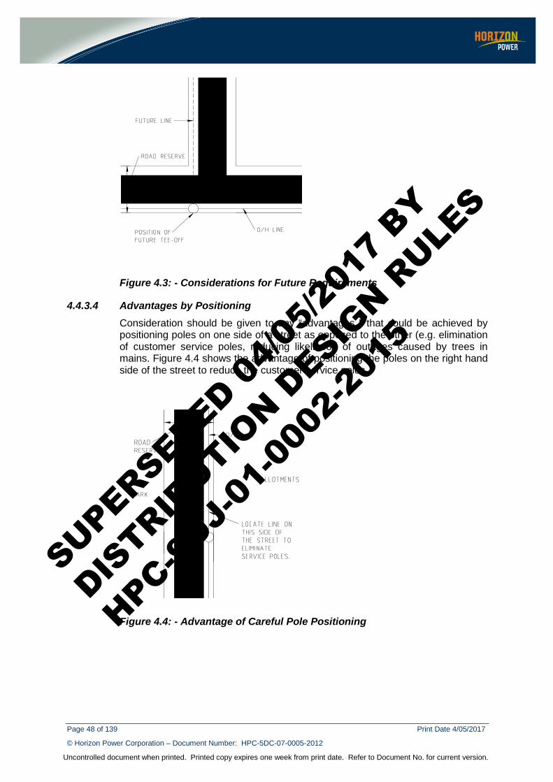
Page 48 of 139 Print Date 4/05/2017
© Horizon Power Corporation – Document Number: HPC-5DC-07-0005-2012
Uncontrolled document when printed. Printed copy expires one week from print date. Refer to Document No. for current version.
Figure 4.3: - Considerations for Future Requirements
4.4.3.4 Advantages by Positioning Consideration should be given to any “advantages ” that could be achieved by positioning poles on one side of a street as opposed to the other (e.g. elimination of customer service poles, reducing likelihood of outages caused by trees in mains. Figure 4.4 shows the advantage of positioning the poles on the right hand side of the street to reduce the customer service poles.
Figure 4.4: - Advantage of Careful Pole Positioning
SUPERSEDED 04/0
5/201
7 BY
DISTRIB
UTION D
ESIGN R
ULES
HPC-9DJ-
01-0
002-
2015
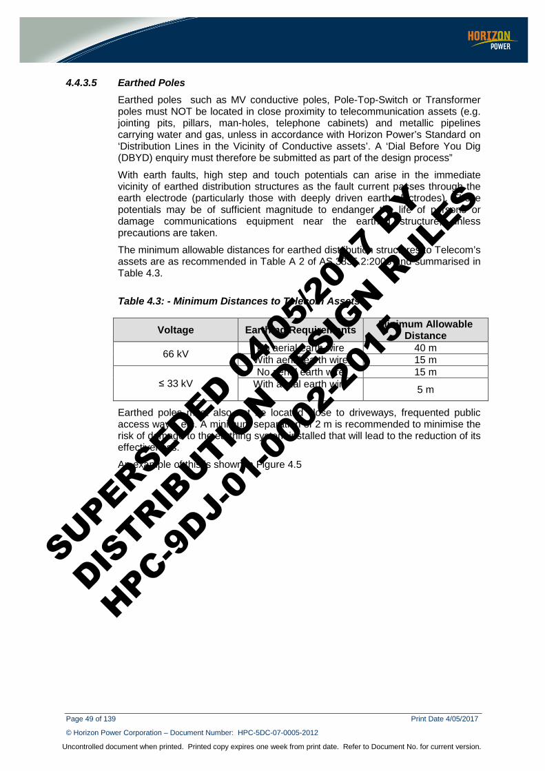
Page 49 of 139 Print Date 4/05/2017
© Horizon Power Corporation – Document Number: HPC-5DC-07-0005-2012
Uncontrolled document when printed. Printed copy expires one week from print date. Refer to Document No. for current version.
4.4.3.5 Earthed Poles Earthed poles such as MV conductive poles, Pole-Top-Switch or Transformer poles must NOT be located in close proximity to telecommunication assets (e.g. jointing pits, pillars, man-holes, telephone cabinets) and metallic pipelines carrying water and gas, unless in accordance with Horizon Power’s Standard on ‘Distribution Lines in the Vicinity of Conductive assets’. A ‘Dial Before You Dig (DBYD) enquiry must therefore be submitted as part of the design process”
With earth faults, high step and touch potentials can arise in the immediate vicinity of earthed distribution structures as the fault current passes through the earth electrode (particularly those with deeply driven earth electrodes). These potentials may be of sufficient magnitude to endanger the life of persons or damage communications equipment near the earthed structure, unless precautions are taken.
The minimum allowable distances for earthed distribution structures to Telecom’s assets are as recommended in Table A 2 of AS 3835.2:2006 and summarised in Table 4.3.
Table 4.3: - Minimum Distances to Telecom Assets
Voltage Earthing Requirements Minimum Allowable Distance
66 kV No aerial earth wire 40 m With aerial earth wire 15 m
≤ 33 kV No aerial earth wire 15 m
With aerial earth wire 5 m
Earthed poles must also not be located close to driveways, frequented public access ways, etc. A minimum separation of 2 m is recommended to minimise the risk of damage to the earthing system installed that will lead to the reduction of its effectiveness.
An example of this is shown in Figure 4.5
SUPERSEDED 04/0
5/201
7 BY
DISTRIB
UTION D
ESIGN R
ULES
HPC-9DJ-
01-0
002-
2015
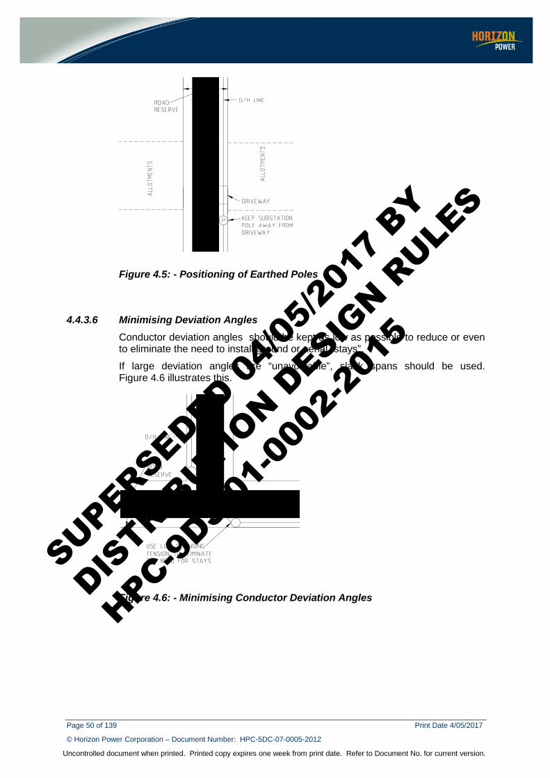
Page 50 of 139 Print Date 4/05/2017
© Horizon Power Corporation – Document Number: HPC-5DC-07-0005-2012
Uncontrolled document when printed. Printed copy expires one week from print date. Refer to Document No. for current version.
Figure 4.5: - Positioning of Earthed Poles
4.4.3.6 Minimising Deviation Angles Conductor deviation angles should be kept as low as possible to reduce or even to eliminate the need to install ground or aerial “stays”.
If large deviation angles are “unavoidable”, slack spans should be used. Figure 4.6 illustrates this.
Figure 4.6: - Minimising Conductor Deviation Angles
SUPERSEDED 04/0
5/201
7 BY
DISTRIB
UTION D
ESIGN R
ULES
HPC-9DJ-
01-0
002-
2015
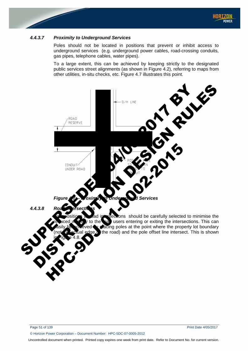
Page 51 of 139 Print Date 4/05/2017
© Horizon Power Corporation – Document Number: HPC-5DC-07-0005-2012
Uncontrolled document when printed. Printed copy expires one week from print date. Refer to Document No. for current version.
4.4.3.7 Proximity to Underground Services Poles should not be located in positions that prevent or inhibit access to underground services (e.g. underground power cables, road-crossing conduits, gas pipes, telephone cables, water pipes).
To a large extent, this can be achieved by keeping strictly to the designated public services street alignments (as shown in Figure 4.2), referring to maps from other utilities, in-situ checks, etc. Figure 4.7 illustrates this point.
Figure 4.7: - Proximity to Underground Services
4.4.3.8 Road Intersections Pole positions at road intersections should be carefully selected to minimise the reduced visibility to the road users entering or exiting the intersections. This can easily be achieved by placing poles at the point where the property lot boundary (not the actual edge of the road) and the pole offset line intersect. This is shown in Figure 4.8.
SUPERSEDED 04/0
5/201
7 BY
DISTRIB
UTION D
ESIGN R
ULES
HPC-9DJ-
01-0
002-
2015
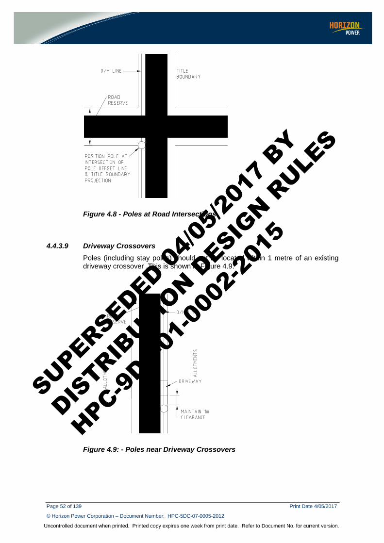
Page 52 of 139 Print Date 4/05/2017
© Horizon Power Corporation – Document Number: HPC-5DC-07-0005-2012
Uncontrolled document when printed. Printed copy expires one week from print date. Refer to Document No. for current version.
Figure 4.8 - Poles at Road Intersections
4.4.3.9 Driveway Crossovers Poles (including stay poles) should not be located within 1 metre of an existing driveway crossover .This is shown in Figure 4.9.
Figure 4.9: - Poles near Driveway Crossovers
SUPERSEDED 04/0
5/201
7 BY
DISTRIB
UTION D
ESIGN R
ULES
HPC-9DJ-
01-0
002-
2015
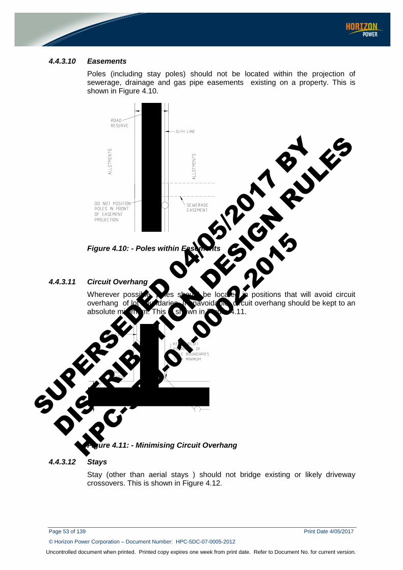
Page 53 of 139 Print Date 4/05/2017
© Horizon Power Corporation – Document Number: HPC-5DC-07-0005-2012
Uncontrolled document when printed. Printed copy expires one week from print date. Refer to Document No. for current version.
4.4.3.10 Easements Poles (including stay poles) should not be located within the projection of sewerage, drainage and gas pipe easements existing on a property. This is shown in Figure 4.10.
Figure 4.10: - Poles within Easements
4.4.3.11 Circuit Overhang Wherever possible, poles should be located in positions that will avoid circuit overhang of lot boundaries. If unavoidable, circuit overhang should be kept to an absolute minimum. This is shown in Figure 4.11.
Figure 4.11: - Minimising Circuit Overhang
4.4.3.12 Stays Stay (other than aerial stays ) should not bridge existing or likely driveway crossovers. This is shown in Figure 4.12.
SUPERSEDED 04/0
5/201
7 BY
DISTRIB
UTION D
ESIGN R
ULES
HPC-9DJ-
01-0
002-
2015
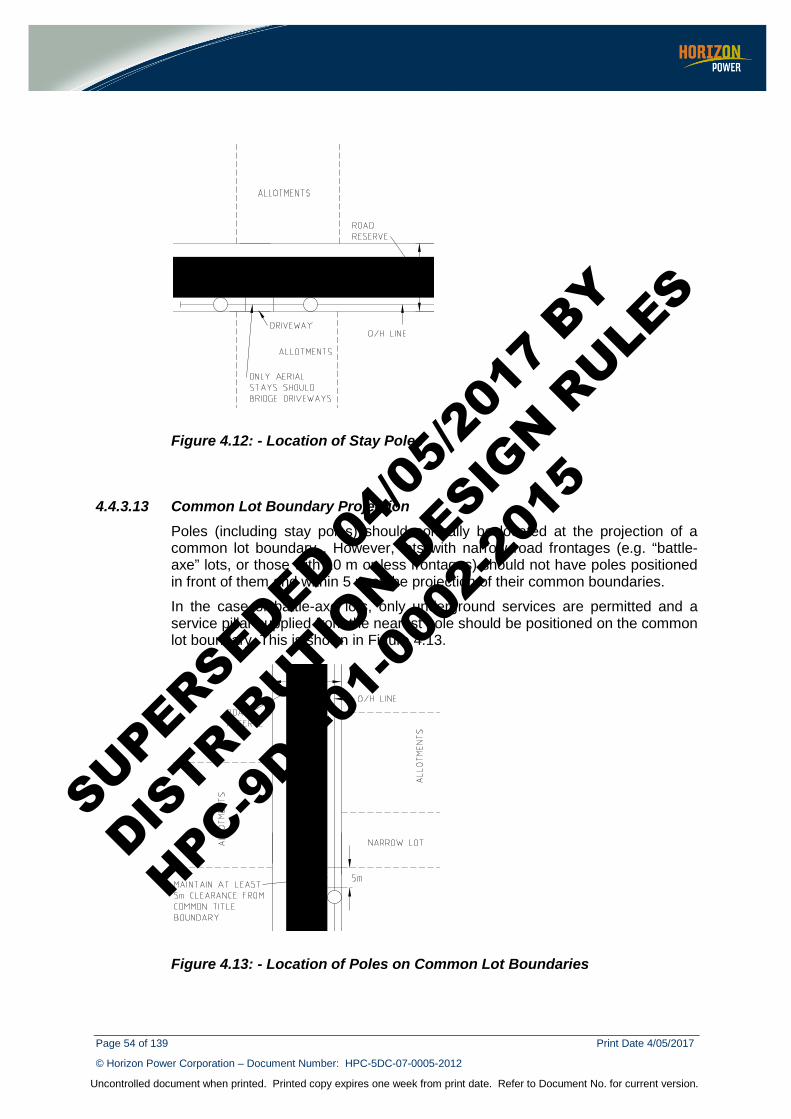
Page 54 of 139 Print Date 4/05/2017
© Horizon Power Corporation – Document Number: HPC-5DC-07-0005-2012
Uncontrolled document when printed. Printed copy expires one week from print date. Refer to Document No. for current version.
Figure 4.12: - Location of Stay Poles
4.4.3.13 Common Lot Boundary Projection Poles (including stay poles) should normally be located at the projection of a common lot boundary . However, lots with narrow road frontages (e.g. “battle-axe” lots, or those with 10 m or less frontages) should not have poles positioned in front of them and within 5 m of the projection of their common boundaries.
In the case of battle-axe lots, only underground services are permitted and a service pillar supplied from the nearest pole should be positioned on the common lot boundary. This is shown in Figure 4.13.
Figure 4.13: - Location of Poles on Common Lot Boundaries
SUPERSEDED 04/0
5/201
7 BY
DISTRIB
UTION D
ESIGN R
ULES
HPC-9DJ-
01-0
002-
2015
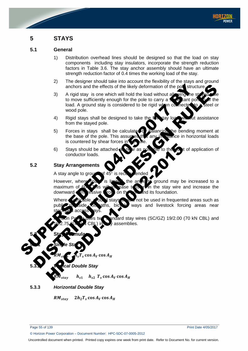
Page 55 of 139 Print Date 4/05/2017
© Horizon Power Corporation – Document Number: HPC-5DC-07-0005-2012
Uncontrolled document when printed. Printed copy expires one week from print date. Refer to Document No. for current version.
5 STAYS
5.1 General 1) Distribution overhead lines should be designed so that the load on stay
components including stay insulators, incorporate the strength reduction factors in Table 3.6. The stay anchor assembly should have an ultimate strength reduction factor of 0.4 times the working load of the stay.
2) The designer should take into account the flexibility of the stays and ground anchors and the effects of the likely deformation of the pole structure.
3) A rigid stay is one which will hold the load without allowing the stayed pole to move sufficiently enough for the pole to carry a significant portion of the load. A ground stay is considered to be rigid when connected to a steel or wood pole.
4) Rigid stays shall be designed to take the full stay load without assistance from the stayed pole.
5) Forces in stays shall be calculated by balancing the bending moment at the base of the pole. This assumes that any imbalance in horizontal loads is countered by shear forces in the pole.
6) Stays should be attached as near as possible to the point of application of conductor loads.
5.2 Stay Arrangements A stay angle to ground of 45° is recommended
However, where space is limited, the angle to ground may be increased to a maximum of 60°. This will increase tension in the stay wire and increase the downward compressive forces on the pole and its foundation.
Where practicable, ground stays should not be used in frequented areas such as public roadside footpaths, bicycle ways and livestock forcing areas near stockyard access ways.
Horizon Power uses two standard stay wires (SC/GZ) 19/2.00 (70 kN CBL) and 19/2.75 (141 kN CBL) in stay assemblies.
5.3 Stay Formulae
5.3.1 Single Stay
𝑹𝑹𝑴𝑴𝑺𝑺𝑺𝑺𝑺𝑺𝒔𝒔 = 𝒉𝒉𝑺𝑺𝑻𝑻𝑺𝑺 𝐏𝐏𝐜𝐜𝐜𝐜𝑨𝑨𝑽𝑽 𝐏𝐏𝐜𝐜𝐜𝐜𝑨𝑨𝑯𝑯
5.3.2 Vertical Double Stay
𝑹𝑹𝑴𝑴𝑺𝑺𝑺𝑺𝑺𝑺𝒔𝒔 = (𝒉𝒉𝑺𝑺𝟏𝟏 + 𝒉𝒉𝑺𝑺𝟐𝟐)𝑻𝑻𝑺𝑺 𝐏𝐏𝐜𝐜𝐜𝐜𝑨𝑨𝑽𝑽 𝐏𝐏𝐜𝐜𝐜𝐜𝑨𝑨𝑯𝑯
5.3.3 Horizontal Double Stay
𝑹𝑹𝑴𝑴𝑺𝑺𝑺𝑺𝑺𝑺𝒔𝒔 = 𝟐𝟐𝒉𝒉𝟐𝟐𝑻𝑻𝑺𝑺 𝐏𝐏𝐜𝐜𝐜𝐜𝑨𝑨𝑽𝑽 𝐏𝐏𝐜𝐜𝐜𝐜𝑨𝑨𝑯𝑯
SUPERSEDED 04/0
5/201
7 BY
DISTRIB
UTION D
ESIGN R
ULES
HPC-9DJ-
01-0
002-
2015
Page 56 of 139 Print Date 4/05/2017
© Horizon Power Corporation – Document Number: HPC-5DC-07-0005-2012
Uncontrolled document when printed. Printed copy expires one week from print date. Refer to Document No. for current version.
5.3.4 Outrigger Stay Outrigger stays are generally not recommended and shall not be used on termination poles. For the design of the outrigger stays, refer to DM# 3739641.
5.3.5 Loads on Poles Refer to section 3.8 for calculation of bending moment for loads on poles.
The minimum embedment depth for poles with stays should be at least 2 m.
5.3.6 Stay Anchorage Ground anchors will move to develop the full passive pressure wedge. If the amount of soil movement has not been specifically determined, a value of 200 mm should be assumed.
It is recommended that ground holding strengths are based on test results rather than calculations. The standard stay design in the Distribution Construction Manual includes anchors with holding strengths equal to or greater than the rest of the stay assembly .
In difficult terrain, such as swampy or marshy ground conditions, special provision needs to be made for anchoring. A swamp type anchor which provides a large cross sectional area should be used. Alternatively, where this does not provide sufficient ground area, stay rods with reinforced concrete block and bulk concrete should be employed.
5.4 List of Symbols RMstay Bending moment support provided by stay
Hs Height of stay above ground (m)
hs1,hs2 Height above ground of each stay in a vertical double stay (m)
Ts Tension in stay (N)
AH Horizontal angle between stay and line of force
AV Angle between stay and horizontal
SUPERSEDED 04/0
5/201
7 BY
DISTRIB
UTION D
ESIGN R
ULES
HPC-9DJ-
01-0
002-
2015
Page 57 of 139 Print Date 4/05/2017
© Horizon Power Corporation – Document Number: HPC-5DC-07-0005-2012
Uncontrolled document when printed. Printed copy expires one week from print date. Refer to Document No. for current version.
5.5 Worked Example In the example in clause 3.8.8.1, determine the size of ground stay required if the ultimate strength requirement is 24 kN and only a 16 kN/12.5 m steel pole is available.
The pole is self supporting for everyday, serviceability and failure containment load conditions without stay. (Pole should not fail due to loss of stay under everyday load)
If ground stay used and attached to the top of pole,
Load required to be supported by stay = 24 kN
Angle of stay = 45° ( transverse and opposing conductor tension loads)
Tension in stay = 24 x 1.414 =34 kN
Component strength factor for distribution stay = 0.8 (Table 3.6)
Ultimate strength of stay = 34 / 0.8 = 42.5 kN – select SC/GZ stay wire 19/2.0 (CBL = 70 kN)
Compressive load in pole due to stay = 24 kN
The compressive strength of 300 mm diameter wood poles is typically around 250 kN with higher strength for steel poles. Hence, the compressive load is generally tolerable. For stayed poles with long length and small diameter, the buckling failure mode of the pole should be considered.
SUPERSEDED 04/0
5/201
7 BY
DISTRIB
UTION D
ESIGN R
ULES
HPC-9DJ-
01-0
002-
2015
Page 58 of 139 Print Date 4/05/2017
© Horizon Power Corporation – Document Number: HPC-5DC-07-0005-2012
Uncontrolled document when printed. Printed copy expires one week from print date. Refer to Document No. for current version.
6 INSULATORS
6.1 Insulator Design Insulators are required to meet electrical, mechanical and pollution withstand requirements during their lifetime. Electrical stresses include power frequency, switching and lightning over voltages and mechanical stresses include the tensile, compressive or cantilever loadings from conductor tension and weight.
Air gap clearance refers to the minimum distance which should be maintained between the live conductor and earthed metal parts of the support to avoid flashover. The minimum air gap clearance (refer to table) has to be maintained even under the conditions of system over-voltages with the insulator strings in the deflected position due to the action of wind pressure. Two types of over voltages which can occur on a distribution overhead line are:
• power frequency over voltages; and • lightning induced over voltages.
6.1.1 Design for Pollution For medium voltage lines, the pollution performance of the insulator usually dictates the amount of insulation required for the particular voltage. When determining the insulation requirements in a contaminated environment, the following criteria need to be considered:
a) Creepage (or leakage) distance b) The ability of the material to endure the electrical activity without being
degraded; and c) The shape of the insulator to assist in reducing the likelihood of
contamination collection and facilitate washing.
The basic concept is to increase the surface creepage distance so that it is long enough to prevent a pollution flashover across the surface of the insulator. Experience has shown that an insulator with an open aerodynamic profile combined with adequate creepage length will give satisfactory service in most locations in Western Australia. Details of a suitable profile are shown in Figure 6.1. Currently polymeric insulators are predominantly used in new installations due their superior performance in polluted environments. Details about insulation co-ordination including design for power frequency and impulse voltages are covered in Chapter 11.
In locations where rainfall is spread throughout the year and aerodynamic profile insulators are not performing satisfactorily fog profile insulators may be considered.
6.1.2 Pins Although pin length may affect electrical characteristics of lines, pins are principally required to meet only mechanical requirements.
SUPERSEDED 04/0
5/201
7 BY
DISTRIB
UTION D
ESIGN R
ULES
HPC-9DJ-
01-0
002-
2015
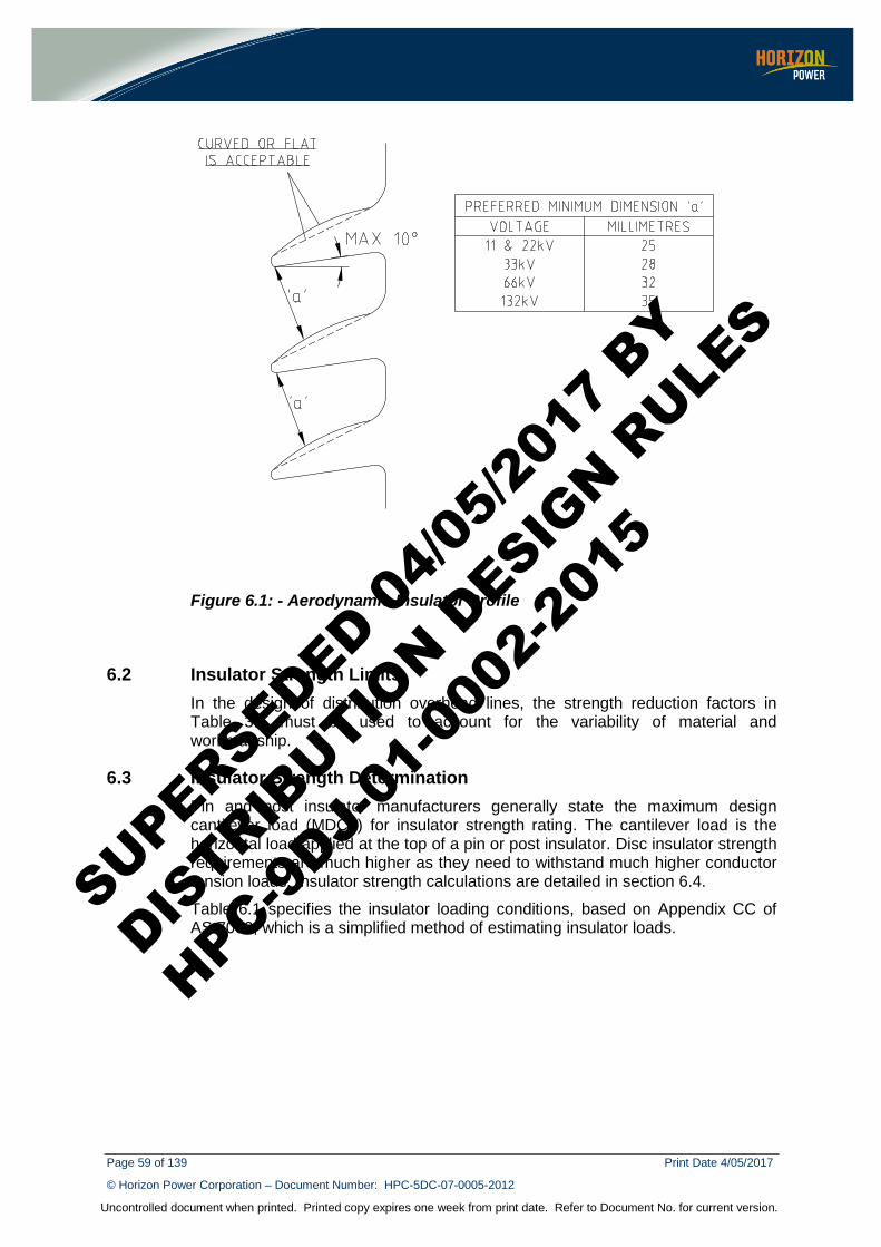
Page 59 of 139 Print Date 4/05/2017
© Horizon Power Corporation – Document Number: HPC-5DC-07-0005-2012
Uncontrolled document when printed. Printed copy expires one week from print date. Refer to Document No. for current version.
Figure 6.1: - Aerodynamic Insulator Profile
6.2 Insulator Strength Limits In the design of distribution overhead lines, the strength reduction factors in Table 3.6 must be used to account for the variability of material and workmanship.
6.3 Insulator Strength Determination Pin and post insulator manufacturers generally state the maximum design cantilever load (MDCL) for insulator strength rating. The cantilever load is the horizontal load applied at the top of a pin or post insulator. Disc insulator strength requirements are much higher as they need to withstand much higher conductor tension loads. Insulator strength calculations are detailed in section 6.4.
Table 6.1 specifies the insulator loading conditions, based on Appendix CC of AS 7000, which is a simplified method of estimating insulator loads.
SUPERSEDED 04/0
5/201
7 BY
DISTRIB
UTION D
ESIGN R
ULES
HPC-9DJ-
01-0
002-
2015
Page 60 of 139 Print Date 4/05/2017
© Horizon Power Corporation – Document Number: HPC-5DC-07-0005-2012
Uncontrolled document when printed. Printed copy expires one week from print date. Refer to Document No. for current version.
Table 6.1 – Insulator Loading Conditions
Limit State Tension Suspension Post and Pin
Everyday Weight span, no wind Weight span, no wind
Serviceability Resultant load at serviceability wind
Resultant load at serviceability wind + longitudinal unbalance load
Ultimate Ultimate Resultant load for ultimate conductor wind transverse load or failure serviceability wind
Resultant load with ultimate transverse wind + longitudinal unbalance load or failure containment load
6.3.1 Standard Insulators Horizon Power uses Strain and Stand-off Insulators:
Strain – 70 kN Strength Rating (creepage -1372 mm and 838 mm options)
Stand-off – 6 kN Strength Rating (creepage -1000 mm)
6.4 Insulator Strength Calculations
6.4.1 Example 1 Determine the strength requirement of a tension ceramic disc insulator used on a 33 kV overhead line with 7/4.75 AAC conductor strung at 20% CBL and 15° C. Assume that the span concerned is a termination span in Esperance.
Tension load (ultimate) is the limiting load condition.
Using the limit state strength condition from clause 3.7.3.1 and
900 kPA is the design wind speed for Esperance (Table 3.5)
Maximum conductor tension at 900 kPA = 8.61 kN (from Overhead line simulation program)
Longitudinal (tension) limit state load = 8.61 x 1.25 = 10.77 kN
Component strength factor for ceramic insulator = 0.8 (Table 3.6)
Minimum required insulator ultimate strength = 10.77 / 0.8 = 13.46 kN
Minimum insulator rating is generally 70 kN, hence disc insulator is suitable.
SUPERSEDED 04/0
5/201
7 BY
DISTRIB
UTION D
ESIGN R
ULES
HPC-9DJ-
01-0
002-
2015
Page 61 of 139 Print Date 4/05/2017
© Horizon Power Corporation – Document Number: HPC-5DC-07-0005-2012
Uncontrolled document when printed. Printed copy expires one week from print date. Refer to Document No. for current version.
6.4.2 Example 2 Determine whether the strength of 11 kV insulators (ALP 11/275) in the example in clause 3.9.3 is adequate to support the overhead line conductors, installed in Esperance.
Using the ultimate limit state strength condition (clause 3.7.2.1)
φRn > Wn + 1.1Gs + 1.25Gc + 1.25Ft
Design wind speed for Esperance = 0.9 kPA (Table 3.5)
Wind span = 47.5 m
Line deviation angle = 15° C
Insulator estimated projected area = 0.02 m2
Insulator drag coefficient = 1.2 (Table 1.6)
Maximum conductor tension at 0.9 kPA = 4.56 kN (from overhead line simulation software)
Conductor weight = 0.576 x 47.5 x 9.8/1000 = 0.27 kN
Conductor weight multiplier = 1.25
Transverse load on insulator
= (1.0 x wind span x SRF x diameter x 0.9) + (1.0 x 0.9 x insulator projected area x insulator drag coefficient) + [1.25 x 2 x 4.56 x sin (15/2)]
= (1.0 x 47.5 x 0.92 x 0.0188 x 0.9) + (1.0 x 0.9 x 0.02 x 1.2) + (1.25 x 2 x 4.56 x 0.13)
= 2.22 kN (This is shown in Figure 6.2)
Everyday Load condition check:
Everyday load on insulator
= 1.25 X (No wind tension @ 5 °C) X sin (15/2)
= 1.25 x 1.76 x 0.13
= 0.286 kN
Component strength factor for ceramic insulator = 0.8 (Table 3.6)
Minimum required insulator ultimate strength = 2.22 / 0.8 = 2.8 kN
Insulator rating is 6 kN, hence the pin insulator is suitable
SUPERSEDED 0
4/05/2
017
BY
DISTRIB
UTION D
ESIGN R
ULES
HPC-9DJ-
01-0
002-
2015
Page 62 of 139 Print Date 4/05/2017
© Horizon Power Corporation – Document Number: HPC-5DC-07-0005-2012
Uncontrolled document when printed. Printed copy expires one week from print date. Refer to Document No. for current version.
Figure 6.2
SUPERSEDED 04/0
5/201
7 BY
DISTRIB
UTION D
ESIGN R
ULES
HPC-9DJ-
01-0
002-
2015
Page 63 of 139 Print Date 4/05/2017
© Horizon Power Corporation – Document Number: HPC-5DC-07-0005-2012
Uncontrolled document when printed. Printed copy expires one week from print date. Refer to Document No. for current version.
7 CROSS-ARMS
7.1 Allowable Stress Limits Distribution overhead lines should be so designed that the cross-arm strength limits in Table 3.5 are not exceeded.
7.1.1 Wood Cross-arms The allowable stress for seasoned wood cross-arms for in service loads shall be calculated using the value of Modulus of rupture for dry wood. However, reference shall be made to AS 1720 for derating factors if the cross-arm has a higher annual average moisture content than 15%.
For green or partially seasoned cross-arms the allowable stress shall be calculated using the value of modulus of rupture for green wood in the former case and an adjusted value in the latter case. Construction loads shall be directly catered for. To calculate in service loads during the period in which the cross-arm is seasoning the return periods specified in AS 1170 “Wind Loading” may be taken into account and the wind pressure reduced accordingly.
Horizon Power uses the following wood cross-arms as standard:
1) 2.1 x 0.1 x 0.1 m treated hard wood cross-arm 2) 2.1 x 0.12 x 0.1 m treated hard wood cross-arm
7.1.2 Steel Cross-arms Horizon Power uses the following cross-arms as standard:
1) 1.9 m unitised steel cross-arm 2) 2.4 m steel cross-arm 3) 3.3 m anti swan cross-arm
7.1.3 Standard Cross-arms Wood cross-arms are used for low voltage only and steel cross-arms for medium voltages.
7.2 Cross-arm Formulae
7.2.1 Cross-arm Strength
7.2.1.1 Intermediate and Angle Cross-arm:
𝑅𝑅𝑀𝑀𝑐𝑐𝑐𝑐𝑐𝑐𝑐𝑐𝑐𝑐𝑐𝑐𝑐𝑐𝑐𝑐 = 10−3(𝑏𝑏 − 𝐵𝐵)(𝑀𝑀2 − 𝐾𝐾2)𝑓𝑓 ÷ 6
7.2.1.2 Termination Cross-arm
𝑹𝑹𝑴𝑴𝒄𝒄𝒄𝒄𝑳𝑳𝑺𝑺𝑺𝑺𝑺𝑺𝒄𝒄𝑴𝑴 = 𝟏𝟏𝟎𝟎−𝟑𝟑𝒃𝒃𝟐𝟐 − 𝑩𝑩𝟐𝟐(𝑺𝑺− 𝑲𝑲)𝒓𝒓 ÷ 𝟔𝟔
Note: Holes only need to be accounted for if they are between the resisting point and the point of application of the load.
SUPERSEDED 04/0
5/201
7 BY
DISTRIB
UTION D
ESIGN R
ULES
HPC-9DJ-
01-0
002-
2015
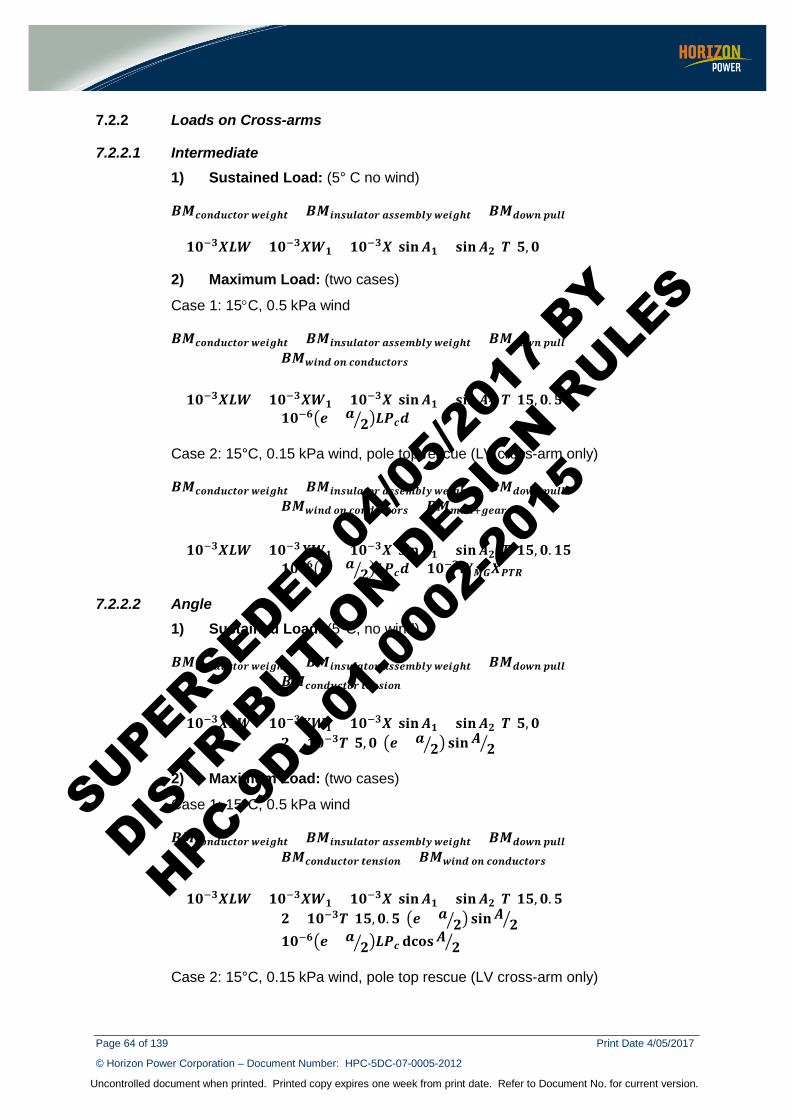
Page 64 of 139 Print Date 4/05/2017
© Horizon Power Corporation – Document Number: HPC-5DC-07-0005-2012
Uncontrolled document when printed. Printed copy expires one week from print date. Refer to Document No. for current version.
7.2.2 Loads on Cross-arms
7.2.2.1 Intermediate 1) Sustained Load: (5° C no wind)
𝑩𝑩𝑴𝑴𝒄𝒄𝑳𝑳𝑺𝑺𝑺𝑺𝑺𝑺𝒄𝒄𝑺𝑺𝑳𝑳𝒄𝒄 𝒘𝒘𝑺𝑺𝑺𝑺𝒘𝒘𝒉𝒉𝑺𝑺 + 𝑩𝑩𝑴𝑴𝑺𝑺𝑺𝑺𝑺𝑺𝑺𝑺𝒊𝒊𝑺𝑺𝑺𝑺𝑳𝑳𝒄𝒄 𝑺𝑺𝑺𝑺𝑺𝑺𝑺𝑺𝑴𝑴𝒃𝒃𝒊𝒊𝒔𝒔 𝒘𝒘𝑺𝑺𝑺𝑺𝒘𝒘𝒉𝒉𝑺𝑺 + 𝑩𝑩𝑴𝑴𝑺𝑺𝑳𝑳𝒘𝒘𝑺𝑺 𝒑𝒑𝑺𝑺𝒊𝒊𝒊𝒊
= 𝟏𝟏𝟎𝟎−𝟑𝟑𝑿𝑿𝑳𝑳𝑿𝑿+ 𝟏𝟏𝟎𝟎−𝟑𝟑𝑿𝑿𝑿𝑿𝟏𝟏 + 𝟏𝟏𝟎𝟎−𝟑𝟑𝑿𝑿(𝐜𝐜𝐬𝐬𝐬𝐬𝑨𝑨𝟏𝟏 + 𝐜𝐜𝐬𝐬𝐬𝐬𝑨𝑨𝟐𝟐)𝑻𝑻(𝟓𝟓,𝟎𝟎)
2) Maximum Load: (two cases)
Case 1: 15°C, 0.5 kPa wind
𝑩𝑩𝑴𝑴𝒄𝒄𝑳𝑳𝑺𝑺𝑺𝑺𝑺𝑺𝒄𝒄𝑺𝑺𝑳𝑳𝒄𝒄 𝒘𝒘𝑺𝑺𝑺𝑺𝒘𝒘𝒉𝒉𝑺𝑺 + 𝑩𝑩𝑴𝑴𝑺𝑺𝑺𝑺𝑺𝑺𝑺𝑺𝒊𝒊𝑺𝑺𝑺𝑺𝑳𝑳𝒄𝒄 𝑺𝑺𝑺𝑺𝑺𝑺𝑺𝑺𝑴𝑴𝒃𝒃𝒊𝒊𝒔𝒔 𝒘𝒘𝑺𝑺𝑺𝑺𝒘𝒘𝒉𝒉𝑺𝑺 + 𝑩𝑩𝑴𝑴𝑺𝑺𝑳𝑳𝒘𝒘𝑺𝑺 𝒑𝒑𝑺𝑺𝒊𝒊𝒊𝒊+ 𝑩𝑩𝑴𝑴𝒘𝒘𝑺𝑺𝑺𝑺𝑺𝑺 𝑳𝑳𝑺𝑺 𝒄𝒄𝑳𝑳𝑺𝑺𝑺𝑺𝑺𝑺𝒄𝒄𝑺𝑺𝑳𝑳𝒄𝒄𝑺𝑺
= 𝟏𝟏𝟎𝟎−𝟑𝟑𝑿𝑿𝑳𝑳𝑿𝑿+ 𝟏𝟏𝟎𝟎−𝟑𝟑𝑿𝑿𝑿𝑿𝟏𝟏 + 𝟏𝟏𝟎𝟎−𝟑𝟑𝑿𝑿(𝐜𝐜𝐬𝐬𝐬𝐬𝑨𝑨𝟏𝟏 + 𝐜𝐜𝐬𝐬𝐬𝐬𝑨𝑨𝟐𝟐)𝑻𝑻(𝟏𝟏𝟓𝟓,𝟎𝟎.𝟓𝟓)+ 𝟏𝟏𝟎𝟎−𝟔𝟔𝑺𝑺 + 𝑺𝑺
𝟐𝟐 𝑳𝑳𝑷𝑷𝒄𝒄𝑺𝑺
Case 2: 15°C, 0.15 kPa wind, pole top rescue (LV cross-arm only)
𝑩𝑩𝑴𝑴𝒄𝒄𝑳𝑳𝑺𝑺𝑺𝑺𝑺𝑺𝒄𝒄𝑺𝑺𝑳𝑳𝒄𝒄 𝒘𝒘𝑺𝑺𝑺𝑺𝒘𝒘𝒉𝒉𝑺𝑺 + 𝑩𝑩𝑴𝑴𝑺𝑺𝑺𝑺𝑺𝑺𝑺𝑺𝒊𝒊𝑺𝑺𝑺𝑺𝑳𝑳𝒄𝒄 𝑺𝑺𝑺𝑺𝑺𝑺𝑺𝑺𝑴𝑴𝒃𝒃𝒊𝒊𝒔𝒔 𝒘𝒘𝑺𝑺𝑺𝑺𝒘𝒘𝒉𝒉𝑺𝑺 + 𝑩𝑩𝑴𝑴𝑺𝑺𝑳𝑳𝒘𝒘𝑺𝑺 𝒑𝒑𝑺𝑺𝒊𝒊𝒊𝒊+ 𝑩𝑩𝑴𝑴𝒘𝒘𝑺𝑺𝑺𝑺𝑺𝑺 𝑳𝑳𝑺𝑺 𝒄𝒄𝑳𝑳𝑺𝑺𝑺𝑺𝑺𝑺𝒄𝒄𝑺𝑺𝑳𝑳𝒄𝒄𝑺𝑺 + 𝑩𝑩𝑴𝑴𝑴𝑴𝑺𝑺𝑺𝑺+𝒘𝒘𝑺𝑺𝑺𝑺𝒄𝒄
= 𝟏𝟏𝟎𝟎−𝟑𝟑𝑿𝑿𝑳𝑳𝑿𝑿+ 𝟏𝟏𝟎𝟎−𝟑𝟑𝑿𝑿𝑿𝑿𝟏𝟏 + 𝟏𝟏𝟎𝟎−𝟑𝟑𝑿𝑿(𝐜𝐜𝐬𝐬𝐬𝐬𝑨𝑨𝟏𝟏 + 𝐜𝐜𝐬𝐬𝐬𝐬𝑨𝑨𝟐𝟐)𝑻𝑻(𝟏𝟏𝟓𝟓,𝟎𝟎.𝟏𝟏𝟓𝟓)+ 𝟏𝟏𝟎𝟎−𝟔𝟔𝑺𝑺 + 𝑺𝑺
𝟐𝟐 𝑳𝑳𝑷𝑷𝒄𝒄𝑺𝑺+ 𝟏𝟏𝟎𝟎−𝟑𝟑𝑿𝑿𝑴𝑴𝑴𝑴𝑿𝑿𝑷𝑷𝑻𝑻𝑹𝑹
7.2.2.2 Angle 1) Sustained Load: (5°C, no wind)
𝑩𝑩𝑴𝑴𝒄𝒄𝑳𝑳𝑺𝑺𝑺𝑺𝑺𝑺𝒄𝒄𝑺𝑺𝑳𝑳𝒄𝒄 𝒘𝒘𝑺𝑺𝑺𝑺𝒘𝒘𝒉𝒉𝑺𝑺 + 𝑩𝑩𝑴𝑴𝑺𝑺𝑺𝑺𝑺𝑺𝑺𝑺𝒊𝒊𝑺𝑺𝑺𝑺𝑳𝑳𝒄𝒄 𝑺𝑺𝑺𝑺𝑺𝑺𝑺𝑺𝑴𝑴𝒃𝒃𝒊𝒊𝒔𝒔 𝒘𝒘𝑺𝑺𝑺𝑺𝒘𝒘𝒉𝒉𝑺𝑺 + 𝑩𝑩𝑴𝑴𝑺𝑺𝑳𝑳𝒘𝒘𝑺𝑺 𝒑𝒑𝑺𝑺𝒊𝒊𝒊𝒊+ 𝑩𝑩𝑴𝑴𝒄𝒄𝑳𝑳𝑺𝑺𝑺𝑺𝑺𝑺𝒄𝒄𝑺𝑺𝑳𝑳𝒄𝒄 𝑺𝑺𝑺𝑺𝑺𝑺𝑺𝑺𝑺𝑺𝑳𝑳𝑺𝑺
= 𝟏𝟏𝟎𝟎−𝟑𝟑𝑿𝑿𝑳𝑳𝑿𝑿+ 𝟏𝟏𝟎𝟎−𝟑𝟑𝑿𝑿𝑿𝑿𝟏𝟏 + 𝟏𝟏𝟎𝟎−𝟑𝟑𝑿𝑿(𝐜𝐜𝐬𝐬𝐬𝐬𝑨𝑨𝟏𝟏 + 𝐜𝐜𝐬𝐬𝐬𝐬𝑨𝑨𝟐𝟐)𝑻𝑻(𝟓𝟓,𝟎𝟎)+ 𝟐𝟐 × 𝟏𝟏𝟎𝟎−𝟑𝟑𝑻𝑻(𝟓𝟓,𝟎𝟎)𝑺𝑺 + 𝑺𝑺
𝟐𝟐 𝐜𝐜𝐬𝐬𝐬𝐬𝑨𝑨 𝟐𝟐
2) Maximum Load: (two cases)
Case 1: 15°C, 0.5 kPa wind
𝑩𝑩𝑴𝑴𝒄𝒄𝑳𝑳𝑺𝑺𝑺𝑺𝑺𝑺𝒄𝒄𝑺𝑺𝑳𝑳𝒄𝒄 𝒘𝒘𝑺𝑺𝑺𝑺𝒘𝒘𝒉𝒉𝑺𝑺 + 𝑩𝑩𝑴𝑴𝑺𝑺𝑺𝑺𝑺𝑺𝑺𝑺𝒊𝒊𝑺𝑺𝑺𝑺𝑳𝑳𝒄𝒄 𝑺𝑺𝑺𝑺𝑺𝑺𝑺𝑺𝑴𝑴𝒃𝒃𝒊𝒊𝒔𝒔 𝒘𝒘𝑺𝑺𝑺𝑺𝒘𝒘𝒉𝒉𝑺𝑺 + 𝑩𝑩𝑴𝑴𝑺𝑺𝑳𝑳𝒘𝒘𝑺𝑺 𝒑𝒑𝑺𝑺𝒊𝒊𝒊𝒊+ 𝑩𝑩𝑴𝑴𝒄𝒄𝑳𝑳𝑺𝑺𝑺𝑺𝑺𝑺𝒄𝒄𝑺𝑺𝑳𝑳𝒄𝒄 𝑺𝑺𝑺𝑺𝑺𝑺𝑺𝑺𝑺𝑺𝑳𝑳𝑺𝑺 + 𝑩𝑩𝑴𝑴𝒘𝒘𝑺𝑺𝑺𝑺𝑺𝑺 𝑳𝑳𝑺𝑺 𝒄𝒄𝑳𝑳𝑺𝑺𝑺𝑺𝑺𝑺𝒄𝒄𝑺𝑺𝑳𝑳𝒄𝒄𝑺𝑺
= 𝟏𝟏𝟎𝟎−𝟑𝟑𝑿𝑿𝑳𝑳𝑿𝑿+ 𝟏𝟏𝟎𝟎−𝟑𝟑𝑿𝑿𝑿𝑿𝟏𝟏 + 𝟏𝟏𝟎𝟎−𝟑𝟑𝑿𝑿(𝐜𝐜𝐬𝐬𝐬𝐬𝑨𝑨𝟏𝟏 + 𝐜𝐜𝐬𝐬𝐬𝐬𝑨𝑨𝟐𝟐)𝑻𝑻(𝟏𝟏𝟓𝟓,𝟎𝟎.𝟓𝟓)+ 𝟐𝟐 × 𝟏𝟏𝟎𝟎−𝟑𝟑𝑻𝑻(𝟏𝟏𝟓𝟓,𝟎𝟎.𝟓𝟓)𝑺𝑺 + 𝑺𝑺
𝟐𝟐 𝐜𝐜𝐬𝐬𝐬𝐬𝑨𝑨 𝟐𝟐+ 𝟏𝟏𝟎𝟎−𝟔𝟔𝑺𝑺 + 𝑺𝑺
𝟐𝟐 𝑳𝑳𝑷𝑷𝒄𝒄 𝐝𝐝𝐏𝐏𝐜𝐜𝐜𝐜𝑨𝑨 𝟐𝟐
Case 2: 15°C, 0.15 kPa wind, pole top rescue (LV cross-arm only)
SUPERSEDED 04/0
5/201
7 BY
DISTRIB
UTION D
ESIGN R
ULES
HPC-9DJ-
01-0
002-
2015
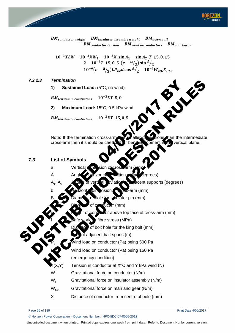
Page 65 of 139 Print Date 4/05/2017
© Horizon Power Corporation – Document Number: HPC-5DC-07-0005-2012
Uncontrolled document when printed. Printed copy expires one week from print date. Refer to Document No. for current version.
𝑩𝑩𝑴𝑴𝒄𝒄𝑳𝑳𝑺𝑺𝑺𝑺𝑺𝑺𝒄𝒄𝑺𝑺𝑳𝑳𝒄𝒄 𝒘𝒘𝑺𝑺𝑺𝑺𝒘𝒘𝒉𝒉𝑺𝑺 + 𝑩𝑩𝑴𝑴𝑺𝑺𝑺𝑺𝑺𝑺𝑺𝑺𝒊𝒊𝑺𝑺𝑺𝑺𝑳𝑳𝒄𝒄 𝑺𝑺𝑺𝑺𝑺𝑺𝑺𝑺𝑴𝑴𝒃𝒃𝒊𝒊𝒔𝒔 𝒘𝒘𝑺𝑺𝑺𝑺𝒘𝒘𝒉𝒉𝑺𝑺 + 𝑩𝑩𝑴𝑴𝑺𝑺𝑳𝑳𝒘𝒘𝑺𝑺 𝒑𝒑𝑺𝑺𝒊𝒊𝒊𝒊+ 𝑩𝑩𝑴𝑴𝒄𝒄𝑳𝑳𝑺𝑺𝑺𝑺𝑺𝑺𝒄𝒄𝑺𝑺𝑳𝑳𝒄𝒄 𝑺𝑺𝑺𝑺𝑺𝑺𝑺𝑺𝑺𝑺𝑳𝑳𝑺𝑺 + 𝑩𝑩𝑴𝑴𝒘𝒘𝑺𝑺𝑺𝑺𝑺𝑺 𝑳𝑳𝑺𝑺 𝒄𝒄𝑳𝑳𝑺𝑺𝑺𝑺𝑺𝑺𝒄𝒄𝑺𝑺𝑳𝑳𝒄𝒄𝑺𝑺 + 𝑩𝑩𝑴𝑴𝑴𝑴𝑺𝑺𝑺𝑺+𝒘𝒘𝑺𝑺𝑺𝑺𝒄𝒄
= 𝟏𝟏𝟎𝟎−𝟑𝟑𝑿𝑿𝑳𝑳𝑿𝑿+ 𝟏𝟏𝟎𝟎−𝟑𝟑𝑿𝑿𝑿𝑿𝟏𝟏 + 𝟏𝟏𝟎𝟎−𝟑𝟑𝑿𝑿(𝐜𝐜𝐬𝐬𝐬𝐬𝑨𝑨𝟏𝟏 + 𝐜𝐜𝐬𝐬𝐬𝐬𝑨𝑨𝟐𝟐)𝑻𝑻(𝟏𝟏𝟓𝟓,𝟎𝟎.𝟏𝟏𝟓𝟓)+ 𝟐𝟐 × 𝟏𝟏𝟎𝟎−𝟑𝟑𝑻𝑻(𝟏𝟏𝟓𝟓,𝟎𝟎.𝟓𝟓)𝑺𝑺 + 𝑺𝑺
𝟐𝟐 𝐜𝐜𝐬𝐬𝐬𝐬𝑨𝑨 𝟐𝟐+ 𝟏𝟏𝟎𝟎−𝟔𝟔𝑺𝑺 + 𝑺𝑺
𝟐𝟐 𝑳𝑳𝑷𝑷𝑬𝑬𝒄𝒄𝑺𝑺𝐏𝐏𝐜𝐜𝐜𝐜𝑨𝑨 𝟐𝟐 + 𝟏𝟏𝟎𝟎−𝟑𝟑𝑿𝑿𝑴𝑴𝑴𝑴𝑿𝑿𝑷𝑷𝑻𝑻𝑹𝑹
7.2.2.3 Termination 1) Sustained Load: (5°C, no wind)
𝑩𝑩𝑴𝑴𝑺𝑺𝑺𝑺𝑺𝑺𝑺𝑺𝑺𝑺𝑳𝑳𝑺𝑺 𝑺𝑺𝑺𝑺 𝒄𝒄𝑳𝑳𝑺𝑺𝑺𝑺𝑺𝑺𝒄𝒄𝑺𝑺𝑳𝑳𝒄𝒄𝑺𝑺 = 𝟏𝟏𝟎𝟎−𝟑𝟑𝑿𝑿𝑻𝑻(𝟓𝟓,𝟎𝟎)
2) Maximum Load: 15°C, 0.5 kPa wind
𝑩𝑩𝑴𝑴𝑺𝑺𝑺𝑺𝑺𝑺𝑺𝑺𝑺𝑺𝑳𝑳𝑺𝑺 𝑺𝑺𝑺𝑺 𝒄𝒄𝐜𝐜𝑺𝑺𝑺𝑺𝑺𝑺𝒄𝒄𝑺𝑺𝑳𝑳𝒄𝒄𝑺𝑺 = 𝟏𝟏𝟎𝟎−𝟑𝟑𝑿𝑿𝑻𝑻(𝟏𝟏𝟓𝟓,𝟎𝟎.𝟓𝟓)
Note: If the termination cross-arm has smaller dimensions than the intermediate cross-arm then it should be checked for bending moment in the vertical plane.
7.3 List of Symbols a Vertical dimension of cross-arm (mm)
A Angle of horizontal deviation of line (degrees)
A1, A2 Angles of vertical deviation of adjacent supports (degrees)
b Horizontal dimension of cross-arm (mm)
B Diameter of hole for insulator pin (mm)
d Diameter of conductor (mm)
e Height of conductor above top face of cross-arm (mm)
f Safe working fibre stress (MPa)
K Diameter of bolt hole for the king bolt (mm)
L Sum of adjacent half spans (m)
Pc Wind load on conductor (Pa) being 500 Pa
PEc Wind load on conductor (Pa) being 150 Pa
(emergency condition)
T(X,Y) Tension in conductor at X°C and Y kPa wind (N)
W Gravitational force on conductor (N/m)
WI Gravitational force on insulator assembly (N/m)
WMG Gravitational force on man and gear (N/m)
X Distance of conductor from centre of pole (mm)
SUPERSEDED 04/0
5/201
7 BY
DISTRIB
UTION D
ESIGN R
ULES
HPC-9DJ-
01-0
002-
2015
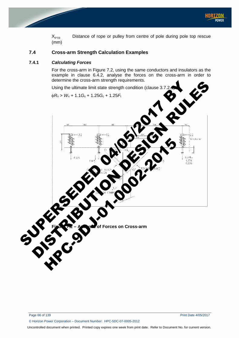
Page 66 of 139 Print Date 4/05/2017
© Horizon Power Corporation – Document Number: HPC-5DC-07-0005-2012
Uncontrolled document when printed. Printed copy expires one week from print date. Refer to Document No. for current version.
XPTR Distance of rope or pulley from centre of pole during pole top rescue (mm)
7.4 Cross-arm Strength Calculation Examples
7.4.1 Calculating Forces For the cross-arm in Figure 7.2, using the same conductors and insulators as the example in clause 6.4.2, analyse the forces on the cross-arm in order to determine the cross-arm strength requirements.
Using the ultimate limit state strength condition (clause 3.7.2.1)
φRn > Wn + 1.1Gs + 1.25Gc + 1.25Ft
Figure 7.2 – Analysis of Forces on Cross-arm
SUPERSEDED 04/0
5/201
7 BY
DISTRIB
UTION D
ESIGN R
ULES
HPC-9DJ-
01-0
002-
2015
Page 67 of 139 Print Date 4/05/2017
© Horizon Power Corporation – Document Number: HPC-5DC-07-0005-2012
Uncontrolled document when printed. Printed copy expires one week from print date. Refer to Document No. for current version.
Conductor weight = 0.576 x 47.5 x 9.8/1000 = 0.27 kN
Factored weight of conductor
= 1.25 Gc = 1.25 x 0.27 = 0.338 kN
Factored weight of insulator
= 1.1 Gs = 1.1 x 20 x 9.8/1000 = 0.196 kN
Factored weight of cross-arm
= 1.1 Gs = 1.1 x 1.35 x 0.1 x 01 x 1000 x 9.8/1000 = 0.145 kN
The reaction forces on the cross-arm are shown as R1, R2 and R3 in Figure 7.2.
For static equilibrium to exist:
Σ Horizontal forces = 0
Σ Vertical forces = 0
Σ Moments about king bolt = 0
Σ Moments about king bolt
= +(2.2 x 3 x 0.35)+ (0.534 x [1.2+0.6]) + (0.145 x 0.675) - (0.145 x 0.675) – (0.534 x 1.2) – (0.325 x R1 )
R1 = 8.1 kN ( equivalent to a 5.7 kN vertical downwards and horizontal forces)
(note that even if cross-arm and insulator weights are ignored there is only a slight variation to R1 )
Σ Horizontal forces = 0
– (2.2 x 3) – 5.7 + R3 = 0
R2 = 12.3 kN
Σ Vertical forces = 0
– (0.534 x 3) – (0.145 x 2) – 5.7 + R2 = 0
R3 = 7.6 Kn
SUPERSEDED 0
4/05/2
017
BY
DISTRIB
UTION D
ESIGN R
ULES
HPC-9DJ-
01-0
002-
2015
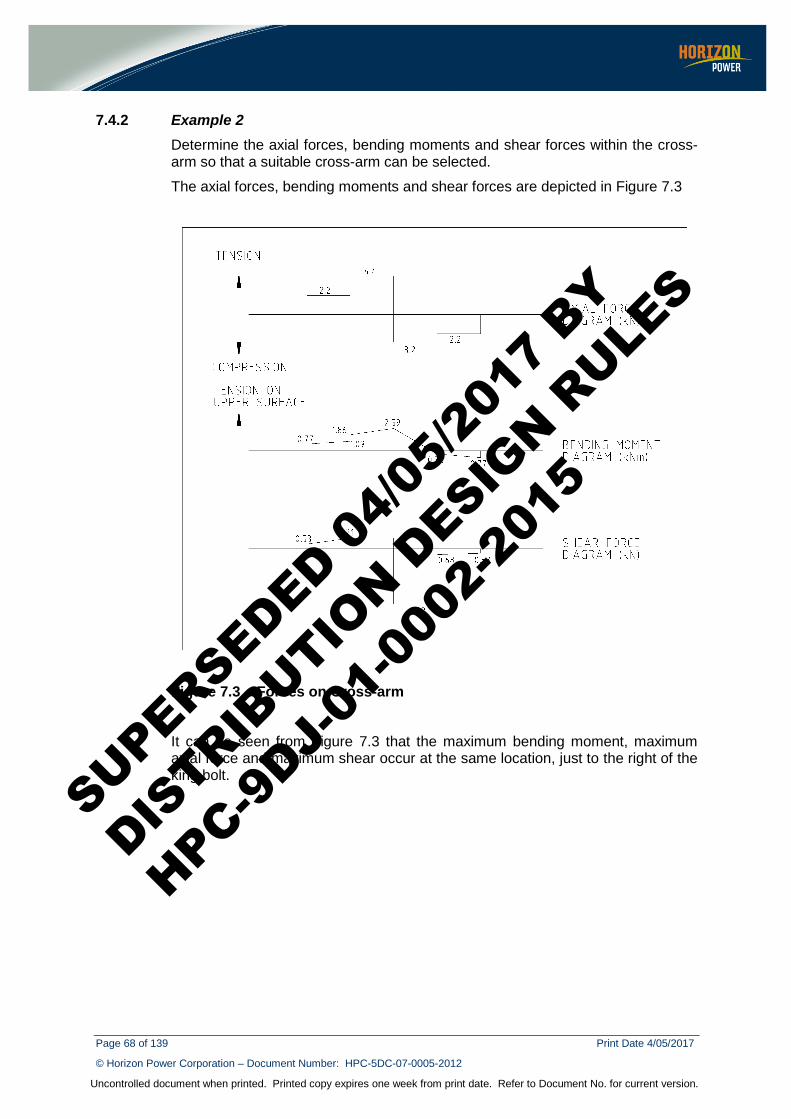
Page 68 of 139 Print Date 4/05/2017
© Horizon Power Corporation – Document Number: HPC-5DC-07-0005-2012
Uncontrolled document when printed. Printed copy expires one week from print date. Refer to Document No. for current version.
7.4.2 Example 2 Determine the axial forces, bending moments and shear forces within the cross-arm so that a suitable cross-arm can be selected.
The axial forces, bending moments and shear forces are depicted in Figure 7.3
Figure 7.3 – Forces on Cross-arm
It can be seen from Figure 7.3 that the maximum bending moment, maximum axial force and maximum shear occur at the same location, just to the right of the king bolt.
SUPERSEDED 0
4/05/2
017
BY
DISTRIB
UTION D
ESIGN R
ULES
HPC-9DJ-
01-0
002-
2015
Page 69 of 139 Print Date 4/05/2017
© Horizon Power Corporation – Document Number: HPC-5DC-07-0005-2012
Uncontrolled document when printed. Printed copy expires one week from print date. Refer to Document No. for current version.
8 CONDUCTORS
8.1 Selection of Conductor Conductor costs amount to between 20 to 40% of the total cost of an overhead line, hence their selection is very important. Bare conductors must be selected considering wire size, shape and material and the following factors:
• Electrical requirements: steady state and transient current ratings, corona discharge, audible noise, radio and television interference, and energy losses
• Mechanical requirements: annealing, drag coefficient, operating temperature, ease of construction (no bird caging or unravelling), permanent elongation, fatigue endurance, conductor diameter, strength and sag
• Environmental: corrosion and lightning damage • Economic factors: Life cycle costs
8.1.1 Electrical Requirements The most important parameter affecting the choice of conductor is its resistance, as it influences voltage regulation, power loss and current rating. The diameter of the conductor affects its inductance and thus its capacity.
The steady state thermal current rating of a conductor is the maximum current inducing the maximum steady state temperature for a given ambient condition and is based on the conductor heat balance equation: Pj + Ps = Pr + Pc
Where Pj = heating due to conductor resistance
Ps = solar heat gain
Pr = radiant cooling
Pc = natural and forced convective cooling
The steady state thermal current rating must be determined for coincident wind velocity and incident angle, daily solar radiation, ambient temperature and conductor surface condition.
The normal (steady state) and short time (emergency) rating of conductors for summer day and night, winter day and night can be determined by using the overhead line simulation program. (Refer to Tables 8.13 and 8.14 for standard conductor ratings).
The emergency rating of a conductor is the maximum current inducing the maximum steady state temperature for a given ambient condition and occurs when a step change in current flow results in a short term conductor temperature change and the
Conductor stored heat = heat gain – heat loss
The conductor maximum operating temperature is limited by required minimum electrical clearances. The time constant for short time ratings is less than 20 minutes.
Factors affecting conductor rating are described below:
SUPERSEDED 04/0
5/201
7 BY
DISTRIB
UTION D
ESIGN R
ULES
HPC-9DJ-
01-0
002-
2015
Page 70 of 139 Print Date 4/05/2017
© Horizon Power Corporation – Document Number: HPC-5DC-07-0005-2012
Uncontrolled document when printed. Printed copy expires one week from print date. Refer to Document No. for current version.
8.1.1.1 Solar Absorption Coefficient Solar absorption coefficient refers to the measure of the incident solar radiation the conductor surface can absorb, ranging from 0 (reflective surface) to 1 (perfectly absorbent surface). Generally 0.6 is appropriate for bright new conductors and 0.9 for old blackened conductors. Considering service life, a value of 0.85 may be used in design.
8.1.1.2 Wind Velocity The rate at which heat dissipates from a conductor is directly proportional to the wind velocity applied to the conductor. As a standard, a wind velocity of 1 m/s shall be used to determine the current carrying capacity of a particular conductor. Increase in wind velocity affects conductor rating significantly.
8.1.1.3 Wind Incident Angle Wind incident angle affects the magnitude of wind loading on conductors. Wind loading shall be assessed under worst case conditions by assuming a wind incident angle perpendicular to the conductors.
8.1.1.4 Temperature
Ambient temperature for Region A is 40 °C (summer) and 15 °C (winter) and for Regions C & D 45 °C (summer) and 35 °C (winter).
Maximum conductor temperature must not exceed 75 °C, to ensure that electrical clearances are maintained.
8.1.1.5 Intensity of Solar Radiation Conductor rating is inversely proportional to solar radiation intensity. Solar radiation intensity is typically set at 1000 W/m2.
8.1.1.6 Ground Reflection Factor This is the ratio of reflected solar radiation to direct incident radiation. It is high for bright reflective surfaces and is generally taken as 0.2, unless a higher value is warranted in particular areas.
8.1.2 Mechanical Requirements When subject to increasing loads, conductors and /or tension fittings may exhibit at some level, permanent deformation particularly if the failure mode is ductile; or for wind induced Aeolian vibration, conductors may exhibit wire and/or whole conductor fracture. This level is called the damage limit and conductors and/or tension fittings will be in the damaged state if the conductors and/or tension fittings have exceeded the damage limit.
If the load is further increased, failure of the conductor and/or tension fittings occurs at a level called the failure limit. The conductors and/or tension fittings will be in a failed state if the conductors and/or tension fittings have exceeded the failure limit. These failure limits are illustrated in Figure 8.1 below.
SUPERSEDED 04/0
5/201
7 BY
DISTRIB
UTION D
ESIGN R
ULES
HPC-9DJ-
01-0
002-
2015
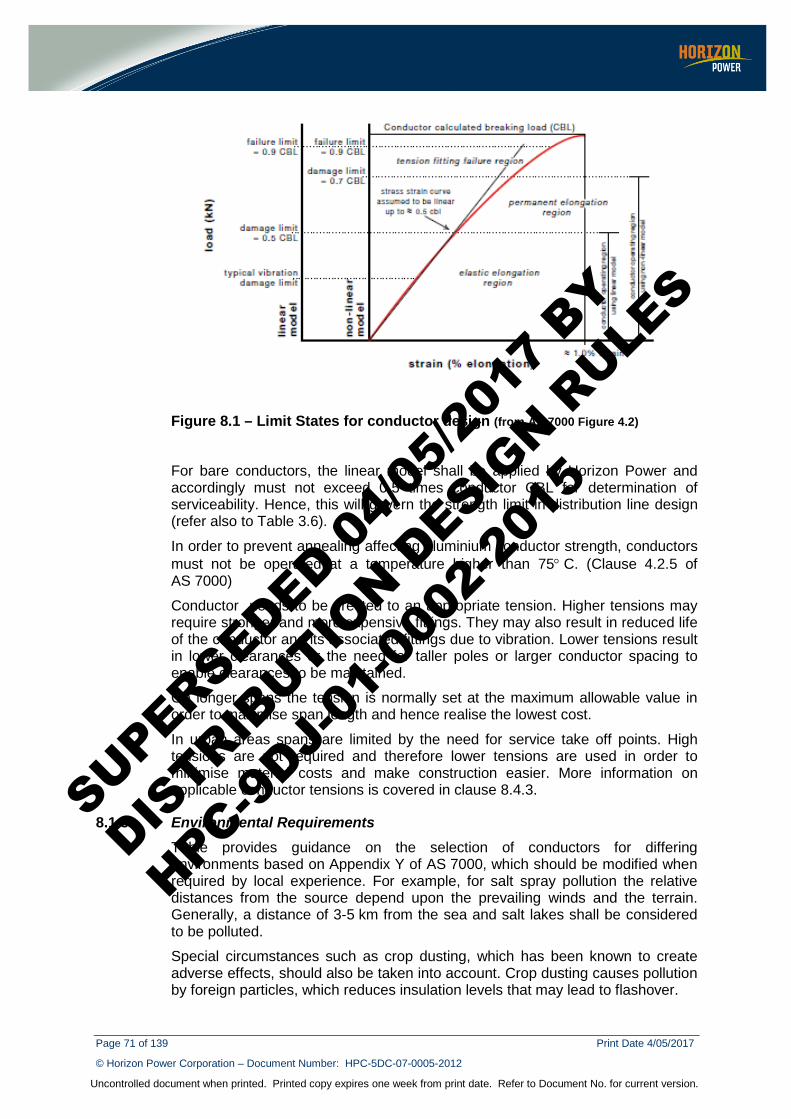
Page 71 of 139 Print Date 4/05/2017
© Horizon Power Corporation – Document Number: HPC-5DC-07-0005-2012
Uncontrolled document when printed. Printed copy expires one week from print date. Refer to Document No. for current version.
Figure 8.1 – Limit States for conductor design (from AS 7000 Figure 4.2)
For bare conductors, the linear model shall be applied by Horizon Power and accordingly must not exceed 0.5 times conductor CBL for determination of serviceability. Hence, this will govern the strength limit in distribution line design (refer also to Table 3.6).
In order to prevent annealing affecting aluminium conductor strength, conductors must not be operated at a temperature higher than 75° C. (Clause 4.2.5 of AS 7000)
Conductor needs to be erected to an appropriate tension. Higher tensions may require stronger and more expensive fittings. They may also result in reduced life of the conductor and its associated fittings due to vibration. Lower tensions result in lower clearances or the need for taller poles or larger conductor spacing to enable clearances to be maintained.
On longer spans the tension is normally set at the maximum allowable value in order to maximise span length and hence realise the lowest cost.
In urban areas spans are limited by the need for service take off points. High tensions are not required and therefore lower tensions are used in order to minimise material costs and make construction easier. More information on applicable conductor tensions is covered in clause 8.4.3.
8.1.3 Environmental Requirements Table provides guidance on the selection of conductors for differing environments based on Appendix Y of AS 7000, which should be modified when required by local experience. For example, for salt spray pollution the relative distances from the source depend upon the prevailing winds and the terrain. Generally, a distance of 3-5 km from the sea and salt lakes shall be considered to be polluted.
Special circumstances such as crop dusting, which has been known to create adverse effects, should also be taken into account. Crop dusting causes pollution by foreign particles, which reduces insulation levels that may lead to flashover.
SUPERSEDED 04/0
5/201
7 BY
DISTRIB
UTION D
ESIGN R
ULES
HPC-9DJ-
01-0
002-
2015
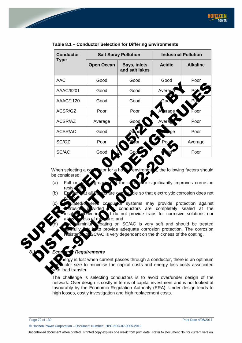
Page 72 of 139 Print Date 4/05/2017
© Horizon Power Corporation – Document Number: HPC-5DC-07-0005-2012
Uncontrolled document when printed. Printed copy expires one week from print date. Refer to Document No. for current version.
Table 8.1 – Conductor Selection for Differing Environments
Conductor Type
Salt Spray Pollution Industrial Pollution
Open Ocean Bays, inlets and salt lakes
Acidic Alkaline
AAC Good Good Good Poor
AAAC/6201 Good Good Average Poor
AAAC/1120 Good Good Good Poor
ACSR/GZ Poor Poor Average Poor
ACSR/AZ Average Good Average Poor
ACSR/AC Good Good Average Poor
SC/GZ Poor Poor Poor Average
SC/AC Good Good Good Poor
When selecting a conductor for a hostile environment, the following factors should be considered:
(a) Full or partial greasing of the conductor significantly improves corrosion resistance.
(b) Ensure that all fittings are compatible so that electrolytic corrosion does not occur.
(c) Insulated/covered conductor systems may provide protection against corrosion provided the conductors are completely sealed at the insulation/covering and do not provide traps for corrosive solutions nor allow ingress of moisture; and
(d) The aluminium coating on SC/AC is very soft and should be treated carefully if it is to provide adequate corrosion protection. The corrosion resistance of SC/AC is very dependent on the thickness of the coating.
8.1.4 Economic Requirements As energy is lost when current passes through a conductor, there is an optimum conductor size to minimise the capital costs and energy loss costs associated with load transfer.
The challenge is selecting conductors is to avoid over/under design of the network. Over design is costly in terms of capital investment and is not looked at favourably by the Economic Regulation Authority (ERA). Under design leads to high losses, costly investigation and high replacement costs.
SUPERSEDED 04/0
5/201
7 BY
DISTRIB
UTION D
ESIGN R
ULES
HPC-9DJ-
01-0
002-
2015
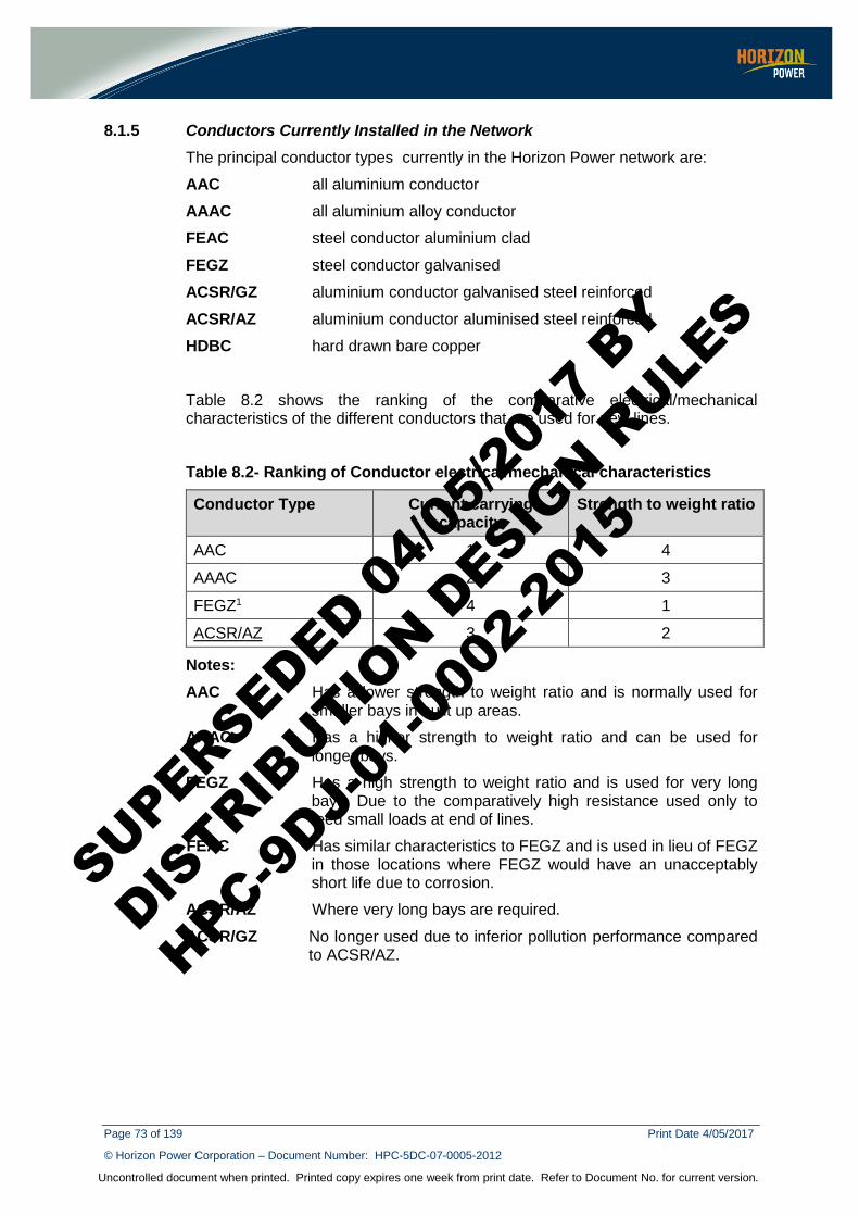
Page 73 of 139 Print Date 4/05/2017
© Horizon Power Corporation – Document Number: HPC-5DC-07-0005-2012
Uncontrolled document when printed. Printed copy expires one week from print date. Refer to Document No. for current version.
8.1.5 Conductors Currently Installed in the Network The principal conductor types currently in the Horizon Power network are:
AAC all aluminium conductor
AAAC all aluminium alloy conductor
FEAC steel conductor aluminium clad
FEGZ steel conductor galvanised
ACSR/GZ aluminium conductor galvanised steel reinforced
ACSR/AZ aluminium conductor aluminised steel reinforced
HDBC hard drawn bare copper
Table 8.2 shows the ranking of the comparative electrical/mechanical characteristics of the different conductors that are used for new lines.
Table 8.2- Ranking of Conductor electrical/mechanical characteristics
Conductor Type Current carrying capacity
Strength to weight ratio
AAC 1 4
AAAC 2 3
FEGZ1 4 1
ACSR/AZ 3 2
Notes: AAC Has a lower strength to weight ratio and is normally used for
smaller bays in built up areas.
AAAC Has a higher strength to weight ratio and can be used for longer bays.
FEGZ Has a high strength to weight ratio and is used for very long bays. Due to the comparatively high resistance used only to feed small loads at end of lines.
FEAC Has similar characteristics to FEGZ and is used in lieu of FEGZ in those locations where FEGZ would have an unacceptably short life due to corrosion.
ACSR/AZ Where very long bays are required. ACSR/GZ No longer used due to inferior pollution performance compared
to ACSR/AZ.
SUPERSEDED 04/0
5/201
7 BY
DISTRIB
UTION D
ESIGN R
ULES
HPC-9DJ-
01-0
002-
2015
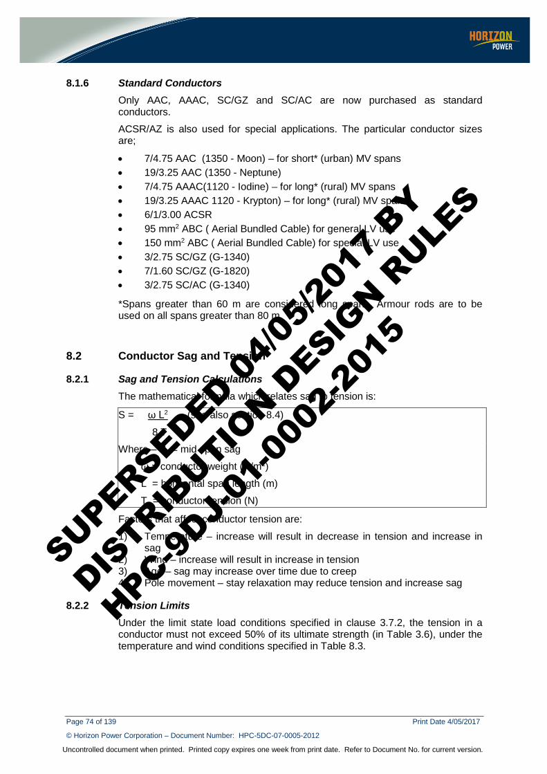
Page 74 of 139 Print Date 4/05/2017
© Horizon Power Corporation – Document Number: HPC-5DC-07-0005-2012
Uncontrolled document when printed. Printed copy expires one week from print date. Refer to Document No. for current version.
8.1.6 Standard Conductors Only AAC, AAAC, SC/GZ and SC/AC are now purchased as standard conductors.
ACSR/AZ is also used for special applications. The particular conductor sizes are;
• 7/4.75 AAC (1350 - Moon) – for short* (urban) MV spans • 19/3.25 AAC (1350 - Neptune) • 7/4.75 AAAC(1120 - Iodine) – for long* (rural) MV spans • 19/3.25 AAAC 1120 - Krypton) – for long* (rural) MV spans • 6/1/3.00 ACSR • 95 mm2 ABC ( Aerial Bundled Cable) for general LV use • 150 mm2 ABC ( Aerial Bundled Cable) for special LV use • 3/2.75 SC/GZ (G-1340) • 7/1.60 SC/GZ (G-1820) • 3/2.75 SC/AC (G-1340)
*Spans greater than 60 m are considered long spans. Armour rods are to be used on all spans greater than 80 m.
8.2 Conductor Sag and Tension
8.2.1 Sag and Tension Calculations The mathematical formula which relates sag to tension is:
S = ω L2 (see also section 8.4)
8 T
Where – S = mid span sag
ω = conductor weight (N/m2)
L = horizontal span length (m)
T = conductor tension (N)
Factors that affect conductor tension are:
1) Temperature – increase will result in decrease in tension and increase in sag
2) Wind – increase will result in increase in tension 3) Age – sag may increase over time due to creep 4) Pole movement – stay relaxation may reduce tension and increase sag
8.2.2 Tension Limits Under the limit state load conditions specified in clause 3.7.2, the tension in a conductor must not exceed 50% of its ultimate strength (in Table 3.6), under the temperature and wind conditions specified in Table 8.3.
SUPERSEDED 04/0
5/201
7 BY
DISTRIB
UTION D
ESIGN R
ULES
HPC-9DJ-
01-0
002-
2015
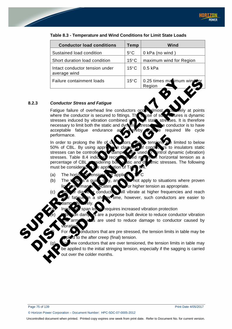
Page 75 of 139 Print Date 4/05/2017
© Horizon Power Corporation – Document Number: HPC-5DC-07-0005-2012
Uncontrolled document when printed. Printed copy expires one week from print date. Refer to Document No. for current version.
Table 8.3 - Temperature and Wind Conditions for Limit State Loads
Conductor load conditions Temp Wind
Sustained load condition 5°C 0 kPa (no wind )
Short duration load condition 15°C maximum wind for Region
Intact conductor tension under average wind
15°C 0.5 kPa
Failure containment loads 15°C 0.25 times maximum wind for Region
8.2.3 Conductor Stress and Fatigue Fatigue failure of overhead line conductors occur almost exclusively at points where the conductor is secured to fittings. The cause of such failures is dynamic stresses induced by vibration combined with high static stresses. It is therefore necessary to limit both the static and dynamic stresses if the conductor is to have acceptable fatigue endurance and thereby provide required life cycle performance.
In order to prolong the life of conductors, design tensions are limited to below 50% of CBL. By using appropriate clamping of conductors to insulators static stresses can be controlled and dampers are used to control dynamic (vibration) stresses. Table 8.4 indicates recommended maximum horizontal tension as a percentage of CBL considering both static and dynamic stresses. The following must be considered in the application of Table 8.4.
(a) The horizontal tensions are applied at 15°C (b) The table is a guide only, and need not apply to situations where proven
line performance indicates a lower or higher tension as appropriate. (c) Smaller diameter conductors will vibrate at higher frequencies and reach
their fatigue in a shorter time, however, such conductors are easier to damp effectively.
(d) Increased span length requires increased vibration protection (e) Vibration dampers are a purpose built device to reduce conductor vibration
and armour rods are used to reduce damage to conductor caused by vibration.
(f) For new conductors that are pre stressed, the tension limits in table may be applied to the after creep (final) tension.
(g) For new conductors that are over tensioned, the tension limits in table may be applied to the initial stringing tension, especially if the sagging is carried out over the colder months.
SUPERSEDED 04/0
5/201
7 BY
DISTRIB
UTION D
ESIGN R
ULES
HPC-9DJ-
01-0
002-
2015
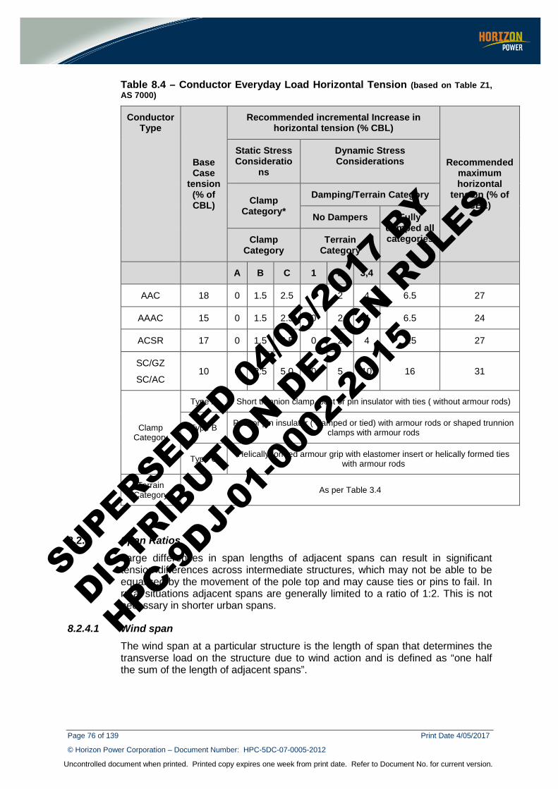
Page 76 of 139 Print Date 4/05/2017
© Horizon Power Corporation – Document Number: HPC-5DC-07-0005-2012
Uncontrolled document when printed. Printed copy expires one week from print date. Refer to Document No. for current version.
Table 8.4 – Conductor Everyday Load Horizontal Tension (based on Table Z1, AS 7000)
Conductor Type
Base Case
tension (% of CBL)
Recommended incremental Increase in horizontal tension (% CBL)
Recommended maximum horizontal
tension (% of CBL)
Static Stress Consideratio
ns
Dynamic Stress Considerations
Clamp Category*
Damping/Terrain Category
No Dampers Fully damped all categories Clamp
Category Terrain
Category
A B C 1 2 3,4
AAC 18 0 1.5 2.5 0 2 4 6.5 27
AAAC 15 0 1.5 2.5 0 2 4 6.5 24
ACSR 17 0 1.5 2.5 0 2 4 7.5 27
SC/GZ
SC/AC 10 0 2.5 5.0 0 5 10 16 31
Clamp Category
Type A Short trunnion clamp, post or pin insulator with ties ( without armour rods)
Type B Post or pin insulator ( clamped or tied) with armour rods or shaped trunnion clamps with armour rods
Type C Helically formed armour grip with elastomer insert or helically formed ties with armour rods
Terrain Category As per Table 3.4
8.2.4 Span Ratios Large differences in span lengths of adjacent spans can result in significant tension differences across intermediate structures, which may not be able to be equalised by the movement of the pole top and may cause ties or pins to fail. In rural situations adjacent spans are generally limited to a ratio of 1:2. This is not necessary in shorter urban spans.
8.2.4.1 Wind span The wind span at a particular structure is the length of span that determines the transverse load on the structure due to wind action and is defined as “one half the sum of the length of adjacent spans”.
SUPERSEDED 04/0
5/201
7 BY
DISTRIB
UTION D
ESIGN R
ULES
HPC-9DJ-
01-0
002-
2015
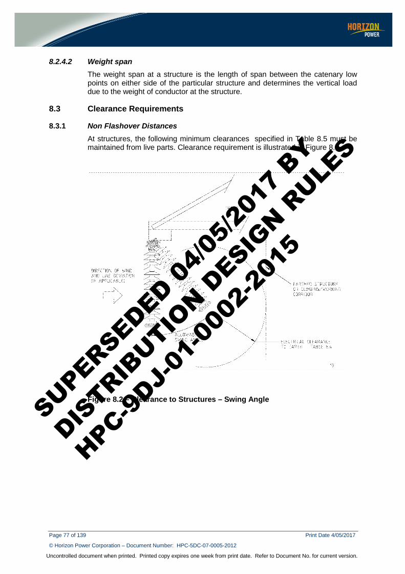
Page 77 of 139 Print Date 4/05/2017
© Horizon Power Corporation – Document Number: HPC-5DC-07-0005-2012
Uncontrolled document when printed. Printed copy expires one week from print date. Refer to Document No. for current version.
8.2.4.2 Weight span The weight span at a structure is the length of span between the catenary low points on either side of the particular structure and determines the vertical load due to the weight of conductor at the structure.
8.3 Clearance Requirements
8.3.1 Non Flashover Distances At structures, the following minimum clearances specified in Table 8.5 must be maintained from live parts. Clearance requirement is illustrated in Figure 8.2
Figure 8.2 – Clearance to Structures – Swing Angle
SUPERSEDED 04/0
5/201
7 BY
DISTRIB
UTION D
ESIGN R
ULES
HPC-9DJ-
01-0
002-
2015
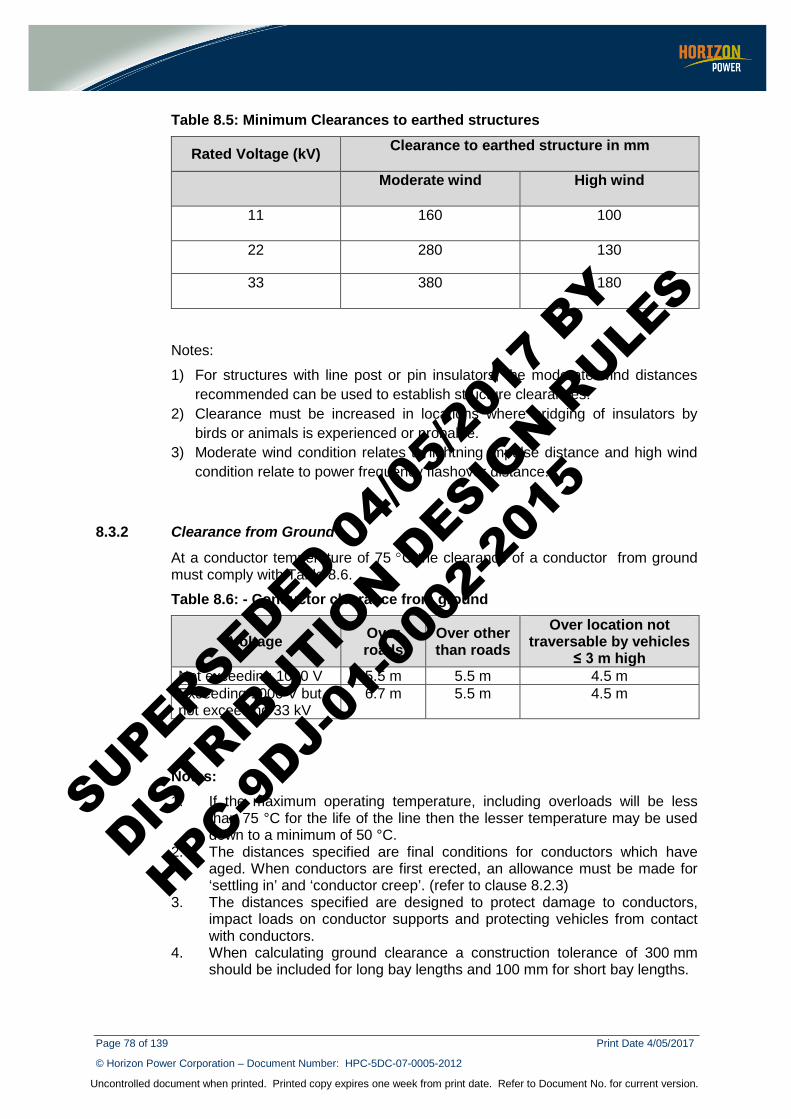
Page 78 of 139 Print Date 4/05/2017
© Horizon Power Corporation – Document Number: HPC-5DC-07-0005-2012
Uncontrolled document when printed. Printed copy expires one week from print date. Refer to Document No. for current version.
Table 8.5: Minimum Clearances to earthed structures
Rated Voltage (kV) Clearance to earthed structure in mm
Moderate wind High wind
11 160 100
22 280 130
33 380 180
Notes:
1) For structures with line post or pin insulators, the moderate wind distances recommended can be used to establish structure clearances.
2) Clearance must be increased in locations where bridging of insulators by birds or animals is experienced or probable.
3) Moderate wind condition relates to lightning impulse distance and high wind condition relate to power frequency flashover distance.
8.3.2 Clearance from Ground
At a conductor temperature of 75 °C the clearance of a conductor from ground must comply with Table 8.6.
Table 8.6: - Conductor clearance from ground
Voltage Over roads
Over other than roads
Over location not traversable by vehicles
≤ 3 m high Not exceeding 1000 V 5.5 m 5.5 m 4.5 m Exceeding 1000 V but not exceeding 33 kV
6.7 m 5.5 m 4.5 m
Notes: 1. If the maximum operating temperature, including overloads will be less
than 75 °C for the life of the line then the lesser temperature may be used down to a minimum of 50 °C.
2. The distances specified are final conditions for conductors which have aged. When conductors are first erected, an allowance must be made for ‘settling in’ and ‘conductor creep’. (refer to clause 8.2.3)
3. The distances specified are designed to protect damage to conductors, impact loads on conductor supports and protecting vehicles from contact with conductors.
4. When calculating ground clearance a construction tolerance of 300 mm should be included for long bay lengths and 100 mm for short bay lengths.
SUPERSEDED 04/0
5/201
7 BY
DISTRIB
UTION D
ESIGN R
ULES
HPC-9DJ-
01-0
002-
2015
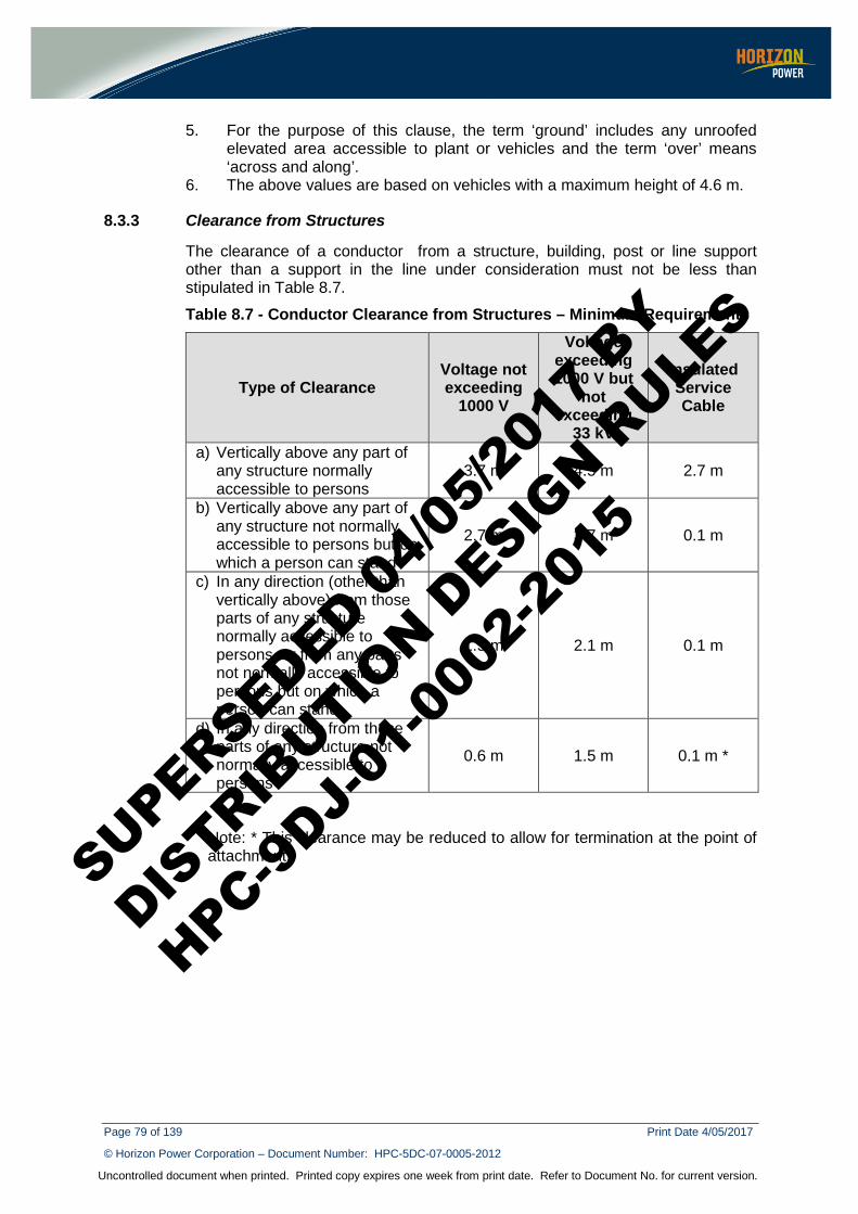
Page 79 of 139 Print Date 4/05/2017
© Horizon Power Corporation – Document Number: HPC-5DC-07-0005-2012
Uncontrolled document when printed. Printed copy expires one week from print date. Refer to Document No. for current version.
5. For the purpose of this clause, the term ‘ground’ includes any unroofed elevated area accessible to plant or vehicles and the term ‘over’ means ‘across and along’.
6. The above values are based on vehicles with a maximum height of 4.6 m.
8.3.3 Clearance from Structures
The clearance of a conductor from a structure, building, post or line support other than a support in the line under consideration must not be less than stipulated in Table 8.7.
Table 8.7 - Conductor Clearance from Structures – Minimum Requirements
Type of Clearance Voltage not exceeding
1000 V
Voltage exceeding 1000 V but
not exceeding
33 kV
Insulated Service Cable
a) Vertically above any part of any structure normally accessible to persons
3.7 m 4.5 m 2.7 m
b) Vertically above any part of any structure not normally accessible to persons but on which a person can stand
2.7 m 3.7 m 0.1 m
c) In any direction (other than vertically above) from those parts of any structure normally accessible to persons, or from any parts not normally accessible to persons but on which a person can stand
1.5 m 2.1 m 0.1 m
d) In any direction from those parts of any structure not normally accessible to persons
0.6 m 1.5 m 0.1 m *
Note: * This clearance may be reduced to allow for termination at the point of attachment.
SUPERSEDED 04/0
5/201
7 BY
DISTRIB
UTION D
ESIGN R
ULES
HPC-9DJ-
01-0
002-
2015

Page 80 of 139 Print Date 4/05/2017
© Horizon Power Corporation – Document Number: HPC-5DC-07-0005-2012
Uncontrolled document when printed. Printed copy expires one week from print date. Refer to Document No. for current version.
Figure 8.3: - Illustration of the application of structure clearances in Table 8-6
Figure 8.4 – Easement Clearances
SUPERSEDED 04/0
5/201
7 BY
DISTRIB
UTION D
ESIGN R
ULES
HPC-9DJ-
01-0
002-
2015
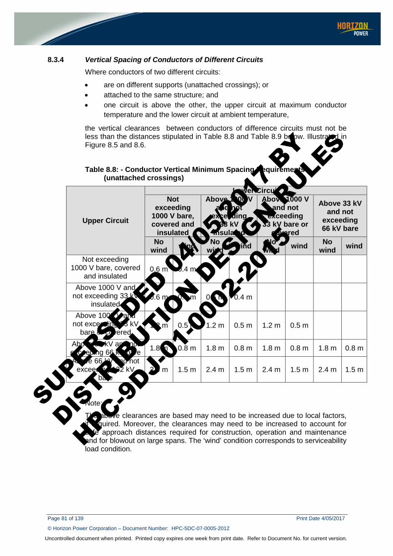
Page 81 of 139 Print Date 4/05/2017
© Horizon Power Corporation – Document Number: HPC-5DC-07-0005-2012
Uncontrolled document when printed. Printed copy expires one week from print date. Refer to Document No. for current version.
8.3.4 Vertical Spacing of Conductors of Different Circuits Where conductors of two different circuits:
• are on different supports (unattached crossings); or • attached to the same structure; and • one circuit is above the other, the upper circuit at maximum conductor
temperature and the lower circuit at ambient temperature,
the vertical clearances between conductors of difference circuits must not be less than the distances stipulated in Table 8.8 and Table 8.9 below. Illustrated in Figure 8.5 and 8.6.
Table 8.8: - Conductor Vertical Minimum Spacing Requirements (unattached crossings)
Upper Circuit
Lower Circuit Not
exceeding 1000 V bare, covered and
insulated
Above 1000 V and not
exceeding 33 kV
insulated
Above 1000 V and not
exceeding 33 kV bare or
covered
Above 33 kV and not
exceeding 66 kV bare
No wind wind No
wind wind No wind wind No
wind wind
Not exceeding 1000 V bare, covered
and insulated 0.6 m 0.4 m
Above 1000 V and not exceeding 33 kV
insulated 0.6 m 0.4 m 0.6 m 0.4 m
Above 1000 V and not exceeding 33 kV
bare or covered 1.2 m 0.5 m 1.2 m 0.5 m 1.2 m 0.5 m
Above 33 kV and not exceeding 66 kV bare 1.8 m 0.8 m 1.8 m 0.8 m 1.8 m 0.8 m 1.8 m 0.8 m
Above 66 kV and not exceeding 132 kV
bare 2.4 m 1.5 m 2.4 m 1.5 m 2.4 m 1.5 m 2.4 m 1.5 m
Note:
The above clearances are based may need to be increased due to local factors, if required. Moreover, the clearances may need to be increased to account for safe approach distances required for construction, operation and maintenance and for blowout on large spans. The ‘wind’ condition corresponds to serviceability load condition.
SUPERSEDED 04/0
5/201
7 BY
DISTRIB
UTION D
ESIGN R
ULES
HPC-9DJ-
01-0
002-
2015
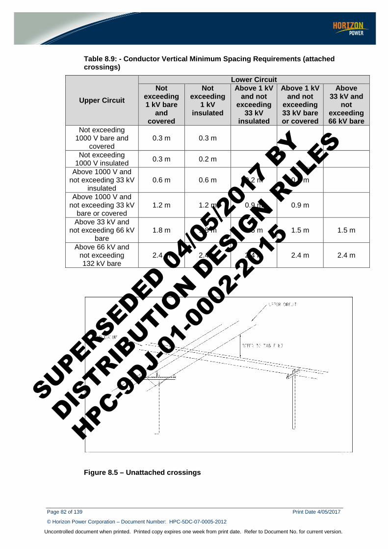
Page 82 of 139 Print Date 4/05/2017
© Horizon Power Corporation – Document Number: HPC-5DC-07-0005-2012
Uncontrolled document when printed. Printed copy expires one week from print date. Refer to Document No. for current version.
Table 8.9: - Conductor Vertical Minimum Spacing Requirements (attached crossings)
Upper Circuit
Lower Circuit Not
exceeding 1 kV bare
and covered
Not exceeding
1 kV insulated
Above 1 kV and not
exceeding 33 kV
insulated
Above 1 kV and not
exceeding 33 kV bare or covered
Above 33 kV and
not exceeding 66 kV bare
Not exceeding 1000 V bare and
covered 0.3 m 0.3 m
Not exceeding 1000 V insulated 0.3 m 0.2 m
Above 1000 V and not exceeding 33 kV
insulated 0.6 m 0.6 m 0.2 m 0.9 m
Above 1000 V and not exceeding 33 kV
bare or covered 1.2 m 1.2 m 0.9 m 0.9 m
Above 33 kV and not exceeding 66 kV
bare 1.8 m 1.8 m 1.5 m 1.5 m 1.5 m
Above 66 kV and not exceeding 132 kV bare
2.4 m 2.4 m 2.4 m 2.4 m 2.4 m
Figure 8.5 – Unattached crossings
SUPERSEDED 04/0
5/201
7 BY
DISTRIB
UTION D
ESIGN R
ULES
HPC-9DJ-
01-0
002-
2015
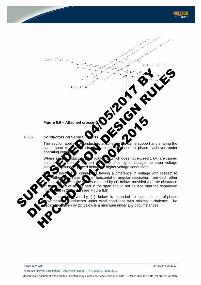
Page 83 of 139 Print Date 4/05/2017
© Horizon Power Corporation – Document Number: HPC-5DC-07-0005-2012
Uncontrolled document when printed. Printed copy expires one week from print date. Refer to Document No. for current version.
Figure 8.6 – Attached crossing
8.3.5 Conductors on Same Supports This section applies to conductors attached to the same support and sharing the same span to prevent circuit to circuit or phase to phase flashover under operating conditions.
Where aerial conductors , the voltage of which does not exceed 1 kV, are carried on the same pole or support as those of a higher voltage the lower voltage conductors must be placed below the higher voltage conductors.
Any two bare aerial conductors having a difference in voltage with respect to each other must have vertical, horizontal or angular separation from each other in accordance with the values required by (1) below, provided that the clearance at the support or at any part in the span should not be less than the separation nominated in (2) below (see Figure 8.8).
The separation given by (1) below is intended to cater for out-of-phase movement of conductors under wind conditions with minimal turbulence. The separation given by (2) below is a minimum under any circumstances.
SUPERSEDED 04/0
5/201
7 BY
DISTRIB
UTION D
ESIGN R
ULES
HPC-9DJ-
01-0
002-
2015
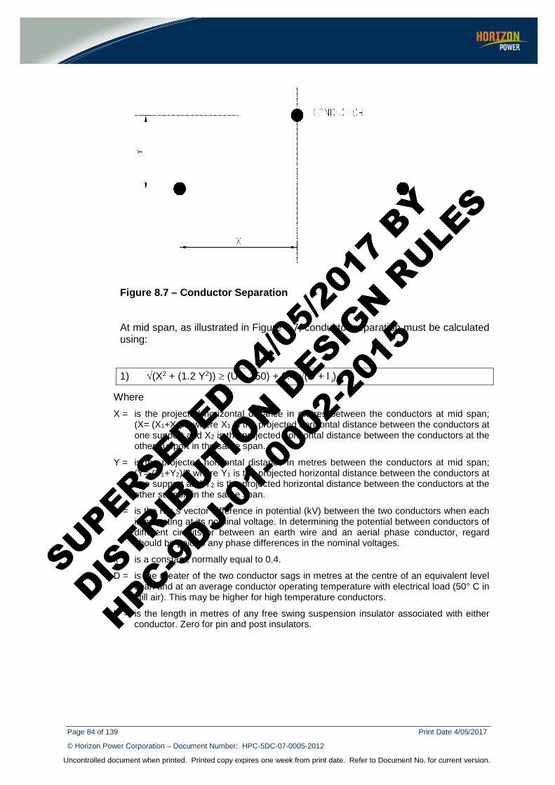
Page 84 of 139 Print Date 4/05/2017
© Horizon Power Corporation – Document Number: HPC-5DC-07-0005-2012
Uncontrolled document when printed. Printed copy expires one week from print date. Refer to Document No. for current version.
Figure 8.7 – Conductor Separation
At mid span, as illustrated in Figure 8.7, conductor separation must be calculated using:
1) √(X2 + (1.2 Y2)) ≥ (U ÷ 150) + 0.4 √(D + l i)
Where X = is the projected horizontal distance in metres between the conductors at mid span;
(X= (X1+X2)/2 where X1 is the projected horizontal distance between the conductors at one support and X2 is the projected horizontal distance between the conductors at the other support in the same span.
Y = is the projected horizontal distance in metres between the conductors at mid span; (Y= (Y1+Y2)/2 where Y1 is the projected horizontal distance between the conductors at one support and Y2 is the projected horizontal distance between the conductors at the other support in the same span.
U = is the r.m.s vector difference in potential (kV) between the two conductors when each is operating at its nominal voltage. In determining the potential between conductors of different circuits or between an earth wire and an aerial phase conductor, regard should be paid to any phase differences in the nominal voltages.
k = is a constant, normally equal to 0.4.
D = is the greater of the two conductor sags in metres at the centre of an equivalent level span and at an average conductor operating temperature with electrical load (50° C in still air). This may be higher for high temperature conductors.
l = is the length in metres of any free swing suspension insulator associated with either conductor. Zero for pin and post insulators.
SUPERSEDED 04/0
5/201
7 BY
DISTRIB
UTION D
ESIGN R
ULES
HPC-9DJ-
01-0
002-
2015
Page 85 of 139 Print Date 4/05/2017
© Horizon Power Corporation – Document Number: HPC-5DC-07-0005-2012
Uncontrolled document when printed. Printed copy expires one week from print date. Refer to Document No. for current version.
For the purposes of this clause an equivalent level span shall mean a span:
a) which has the same span length in the horizontal projection as the original span;
b) in which conductor attachments at supports are in the same horizontal plane;
c) in which the horizontal component of conductor tension is the same as in the original span.
2) At the supports or at any point in the span:
For voltages up to and including 11 kV - 0.38 m
For voltage (U kV) exceeding 11 kV - 0.38 m + 0.01 (U -11) m
Notes:
1) When conductors of different circuits are located vertically one above the other, consideration should be given to the need to prevent clashing of conductors of different circuits under the influence of load current in one or both circuits.
2) This clause is not intended to apply to insulated conductors (with or without earthed screens) of any voltage.
3) The spacing for covered conductors may be reduced provided the covering is adequate to prevent electrical breakdown of the covering when the conductors clash and a risk management strategy is in place to ensure that conductors do not remain entangled for periods beyond what the covering can withstand.
4) Where spacers are used, separation may be less than those specified. It is suggested that the spacer be taken to be a conductor support for the purpose of calculating conductor spacing.
5) The above empirical formula (1) is intended to minimise the risk of conductor clashing, however, circumstances do arise where it is not practicable to give guidance or predict outcomes. Some of these situations involve:
a) Extremely turbulent wind conditions – k to be in the range 0.4 to 0.6
b) The different amount of movement of conductors of different size and type under the same wind conditions
c) Conductor movement under fault conditions (particularly with horizontal construction).
The following k factors are recommended for overhead power lines which have phase to phase clearances of 1200 mm or less at mid span:
i) Extremely turbulent wind conditions – k to be in the range 0.4 to 0.6 ii) High to extreme bushfire prone areas - k to be in the range 0.4 to 0.6 iii) Under high phase to phase fault conditions - k = 0.4 for fault currents
upto 4000 A, 05 for fault currents 4000 A to 6000 A and 0.6 for fault currents above 6000 A
iv) Conductors of different mass/diameter ratios and at different attachment heights – k = 0.4 to 0.6
SUPERSEDED 04/0
5/201
7 BY
DISTRIB
UTION D
ESIGN R
ULES
HPC-9DJ-
01-0
002-
2015

Page 86 of 139 Print Date 4/05/2017
© Horizon Power Corporation – Document Number: HPC-5DC-07-0005-2012
Uncontrolled document when printed. Printed copy expires one week from print date. Refer to Document No. for current version.
In all other situations a k factor of 0.4 is recommended.
6) Mid span clearances may need to be increased in situations where the conductors transition from horizontal to vertical or where the adjacent conductors are of different characteristics (diameter, weight) which can cause out of phase movement.
7) The following situations may also need to be considered when considering spacing of conductors but it is not practicable to provide guidance in this document. Knowledge of local conditions would be required to make design decisions.
a) Aircraft warning devices.
b) Large birds which may collide with conductors, causing them to come together, or whose wingspan is such as to make contact between bare conductors and conducting cross arms.
c) Flocks of birds resting on conductors are known to “lift-off” simultaneously, causing violent conductor movement.
d) Terrain factors that may contribute to aerodynamic lift and/or random motion
e) Spray irrigators; and
f) Safety approach clearances for construction, operation and maintenance
Figure 8.8 – Minimum Conductor Separation – Attached on Same Structure
SUPERSEDED 04/0
5/201
7 BY
DISTRIB
UTION D
ESIGN R
ULES
HPC-9DJ-
01-0
002-
2015
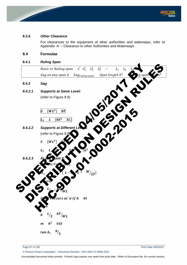
Page 87 of 139 Print Date 4/05/2017
© Horizon Power Corporation – Document Number: HPC-5DC-07-0005-2012
Uncontrolled document when printed. Printed copy expires one week from print date. Refer to Document No. for current version.
8.3.6 Other Clearance For clearances to the equipment of other authorities and waterways, refer to Appendix ‘A’ – Clearance to other Authorities and Waterways.
8.4 Formulae
8.4.1 Ruling Span
𝐵𝐵𝑀𝑀𝑐𝑐𝑀𝑀𝑐𝑐 𝐿𝐿𝑐𝑐 𝑅𝑅𝑀𝑀𝑝𝑝𝑀𝑀𝑊𝑊𝑅𝑅 𝑐𝑐𝑝𝑝𝑀𝑀𝑊𝑊 = √(𝐿𝐿13 + 𝐿𝐿23 + 𝐿𝐿33 + ⋯ ) ÷ (𝐿𝐿1 + 𝐿𝐿2 + 𝐿𝐿3 + ⋯ )
𝑆𝑆𝑀𝑀𝑅𝑅 𝐿𝐿𝑊𝑊 𝑀𝑀𝑊𝑊𝑎𝑎 𝑐𝑐𝑝𝑝𝑀𝑀𝑊𝑊 𝑋𝑋 = 𝑆𝑆𝑀𝑀𝑅𝑅𝑐𝑐𝑟𝑟𝑟𝑟𝑟𝑟𝑟𝑟𝑟𝑟 𝑐𝑐𝑝𝑝𝑐𝑐𝑟𝑟 × (𝑆𝑆𝑝𝑝𝑀𝑀𝑊𝑊 𝑝𝑝𝑝𝑝𝑊𝑊𝑅𝑅𝑐𝑐ℎ 𝑋𝑋2) ÷ (𝑅𝑅𝑀𝑀𝑝𝑝𝑀𝑀𝑊𝑊𝑅𝑅 𝑐𝑐𝑝𝑝𝑀𝑀𝑊𝑊 𝑝𝑝𝑝𝑝𝑊𝑊𝑅𝑅𝑐𝑐ℎ2)
8.4.2 Sag
8.4.2.1 Supports at Same Level: (refer to Figure 8.9)
𝑺𝑺 = 𝑿𝑿𝑳𝑳𝟐𝟐 ÷ 𝟖𝟖𝑻𝑻
𝑳𝑳𝑻𝑻 = 𝑳𝑳 + 𝟖𝟖𝑺𝑺𝟐𝟐 ÷ 𝟑𝟑𝑳𝑳
8.4.2.2 Supports at Different Levels: (refer to Figure 8.9)
𝑺𝑺 = 𝑿𝑿𝑳𝑳𝟐𝟐 ÷ 𝟖𝟖𝑻𝑻
𝑳𝑳𝑻𝑻 = 𝑳𝑳 + 𝑿𝑿𝟐𝟐𝑳𝑳𝟑𝟑 ÷ 𝟐𝟐𝟐𝟐𝑻𝑻𝟐𝟐 + 𝒉𝒉𝟐𝟐 ÷ 𝟐𝟐𝑳𝑳
8.4.2.3 At any Point X: (refer to Figure 8.9)
𝑯𝑯𝑴𝑴 = 𝒉𝒉 + 𝑺𝑺 − (𝑳𝑳 − 𝑺𝑺 − 𝑴𝑴)𝟐𝟐 × 𝑿𝑿𝟐𝟐𝑻𝑻
𝒘𝒘𝒉𝒉𝑺𝑺𝒄𝒄𝑺𝑺
𝑺𝑺 = 𝑳𝑳𝟐𝟐 − 𝒉𝒉𝑻𝑻
𝑿𝑿𝑳𝑳
𝑼𝑼𝒑𝒑𝒊𝒊𝑺𝑺𝒓𝒓𝑺𝑺 𝑳𝑳𝒄𝒄𝒄𝒄𝑺𝑺𝒄𝒄𝑺𝑺 𝑺𝑺𝑺𝑺 ′𝑺𝑺′𝑺𝑺𝒓𝒓 𝒉𝒉 > 𝟐𝟐𝑺𝑺
𝑺𝑺𝒊𝒊𝑺𝑺𝑳𝑳
𝒃𝒃 = 𝑳𝑳𝟐𝟐 + 𝒉𝒉𝑻𝑻
𝑿𝑿𝑳𝑳
𝑴𝑴 = 𝒉𝒉𝟐𝟐 ÷ 𝟏𝟏𝟔𝟔𝑺𝑺
𝑺𝑺𝑺𝑺𝑺𝑺𝑨𝑨𝟏𝟏 = 𝒉𝒉𝑳𝑳
SUPERSEDED 04/0
5/201
7 BY
DISTRIB
UTION D
ESIGN R
ULES
HPC-9DJ-
01-0
002-
2015
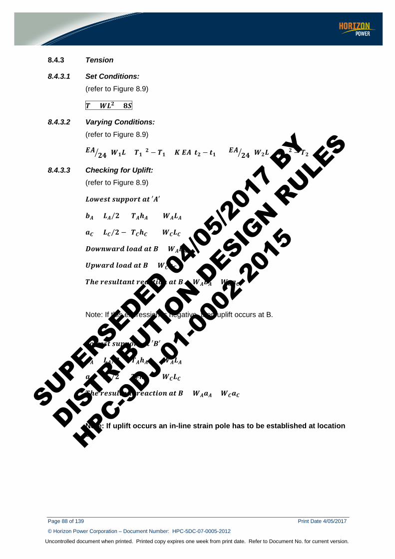
Page 88 of 139 Print Date 4/05/2017
© Horizon Power Corporation – Document Number: HPC-5DC-07-0005-2012
Uncontrolled document when printed. Printed copy expires one week from print date. Refer to Document No. for current version.
8.4.3 Tension
8.4.3.1 Set Conditions: (refer to Figure 8.9)
𝑻𝑻 = 𝑿𝑿𝑳𝑳𝟐𝟐 ÷ 𝟖𝟖𝑺𝑺
8.4.3.2 Varying Conditions: (refer to Figure 8.9)
𝑬𝑬𝑨𝑨𝟐𝟐𝟐𝟐 (𝑿𝑿𝟏𝟏𝑳𝑳 ÷ 𝑻𝑻𝟏𝟏)𝟐𝟐 − 𝑻𝑻𝟏𝟏 + 𝑲𝑲 𝑬𝑬𝑨𝑨(𝑺𝑺𝟐𝟐 − 𝑺𝑺𝟏𝟏) = 𝑬𝑬𝑨𝑨
𝟐𝟐𝟐𝟐 (𝑿𝑿𝟐𝟐𝑳𝑳 ÷ 𝑻𝑻𝟐𝟐)𝟐𝟐 − 𝑻𝑻𝟐𝟐
8.4.3.3 Checking for Uplift: (refer to Figure 8.9)
𝑳𝑳𝑳𝑳𝒘𝒘𝑺𝑺𝑺𝑺𝑺𝑺 𝑺𝑺𝑺𝑺𝒑𝒑𝒑𝒑𝑳𝑳𝒄𝒄𝑺𝑺 𝑺𝑺𝑺𝑺 ′𝑨𝑨′
𝒃𝒃𝑨𝑨 = 𝑳𝑳𝑨𝑨 𝟐𝟐⁄ + (𝑻𝑻𝑨𝑨𝒉𝒉𝑨𝑨) ÷ (𝑿𝑿𝑨𝑨𝑳𝑳𝑨𝑨)
𝑺𝑺𝑪𝑪 = 𝑳𝑳𝑪𝑪 𝟐𝟐⁄ − (𝑻𝑻𝑪𝑪𝒉𝒉𝑪𝑪) ÷ (𝑿𝑿𝑪𝑪𝑳𝑳𝑪𝑪)
𝑫𝑫𝑳𝑳𝒘𝒘𝑺𝑺𝒘𝒘𝑺𝑺𝒄𝒄𝑺𝑺 𝒊𝒊𝑳𝑳𝑺𝑺𝑺𝑺 𝑺𝑺𝑺𝑺 𝑩𝑩 = 𝑿𝑿𝑨𝑨𝒃𝒃𝑨𝑨
𝑼𝑼𝒑𝒑𝒘𝒘𝑺𝑺𝒄𝒄𝑺𝑺 𝒊𝒊𝑳𝑳𝑺𝑺𝑺𝑺 𝑺𝑺𝑺𝑺 𝑩𝑩 = 𝑿𝑿𝑪𝑪𝑺𝑺𝑪𝑪
𝑻𝑻𝒉𝒉𝑺𝑺 𝒄𝒄𝑺𝑺𝑺𝑺𝑺𝑺𝒊𝒊𝑺𝑺𝑺𝑺𝑺𝑺𝑺𝑺 𝒄𝒄𝑺𝑺𝑺𝑺𝒄𝒄𝑺𝑺𝑺𝑺𝑳𝑳𝑺𝑺 𝑺𝑺𝑺𝑺 𝑩𝑩 = 𝑿𝑿𝑨𝑨𝒃𝒃𝑨𝑨 + 𝑿𝑿𝑪𝑪𝑺𝑺𝑪𝑪
Note: If this expression is negative, then uplift occurs at B.
𝑳𝑳𝑳𝑳𝒘𝒘𝑺𝑺𝑺𝑺𝑺𝑺 𝑺𝑺𝑺𝑺𝒑𝒑𝒑𝒑𝑳𝑳𝒄𝒄𝑺𝑺 𝑺𝑺𝑺𝑺 ′𝑩𝑩′
𝑺𝑺𝑨𝑨 = 𝑳𝑳𝑨𝑨 𝟐𝟐⁄ + (𝑻𝑻𝑨𝑨𝒉𝒉𝑨𝑨) ÷ (𝑿𝑿𝑨𝑨𝑳𝑳𝑨𝑨)
𝑺𝑺𝑪𝑪 = 𝑳𝑳𝑪𝑪 𝟐𝟐⁄ + (𝑻𝑻𝑪𝑪𝒉𝒉𝑪𝑪) ÷ (𝑿𝑿𝑪𝑪𝑳𝑳𝑪𝑪)
𝑻𝑻𝒉𝒉𝑺𝑺 𝒄𝒄𝑺𝑺𝑺𝑺𝑺𝑺𝒊𝒊𝑺𝑺𝑺𝑺𝑺𝑺𝑺𝑺 𝒄𝒄𝑺𝑺𝑺𝑺𝒄𝒄𝑺𝑺𝑺𝑺𝑳𝑳𝑺𝑺 𝑺𝑺𝑺𝑺 𝑩𝑩 = 𝑿𝑿𝑨𝑨𝑺𝑺𝑨𝑨 + 𝑿𝑿𝑪𝑪𝑺𝑺𝑪𝑪
Note: If uplift occurs an in-line strain pole has to be established at location B.
SUPERSEDED 04/0
5/201
7 BY
DISTRIB
UTION D
ESIGN R
ULES
HPC-9DJ-
01-0
002-
2015
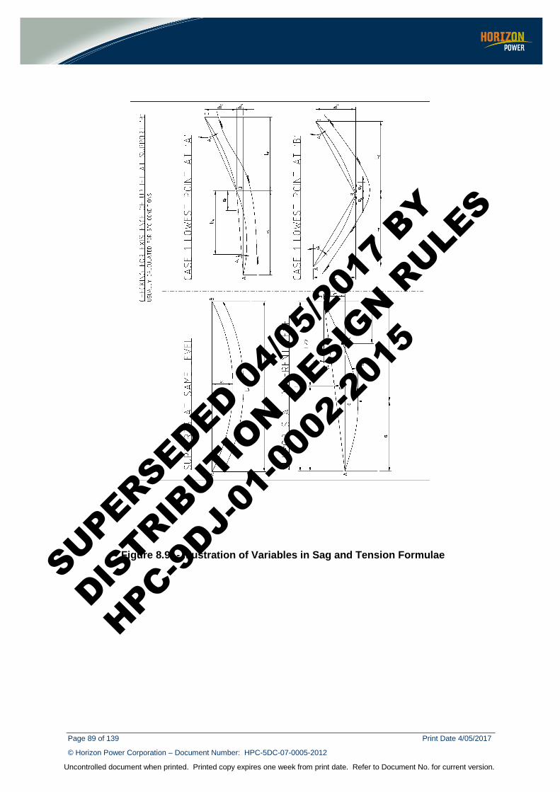
Page 89 of 139 Print Date 4/05/2017
© Horizon Power Corporation – Document Number: HPC-5DC-07-0005-2012
Uncontrolled document when printed. Printed copy expires one week from print date. Refer to Document No. for current version.
Figure 8.9: - Illustration of Variables in Sag and Tension Formulae
SUPERSEDED 04/0
5/201
7 BY
DISTRIB
UTION D
ESIGN R
ULES
HPC-9DJ-
01-0
002-
2015
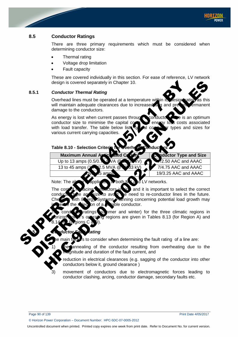
Page 90 of 139 Print Date 4/05/2017
© Horizon Power Corporation – Document Number: HPC-5DC-07-0005-2012
Uncontrolled document when printed. Printed copy expires one week from print date. Refer to Document No. for current version.
8.5 Conductor Ratings There are three primary requirements which must be considered when determining conductor size:
• Thermal rating • Voltage drop limitation • Fault capacity
These are covered individually in this section. For ease of reference, LV network design is covered separately in Chapter 10.
8.5.1 Conductor Thermal Rating Overhead lines must be operated at a temperature within its design rating as this will maintain adequate clearances due to increased sag and prevent permanent damage to the conductors.
As energy is lost when current passes through a conductor, there is an optimum conductor size to minimise the capital costs and energy loss costs associated with load transfer. The table below lists typical conductor types and sizes for various current carrying capacities.
Table 8.10 - Selection Criteria for Overhead Conductors Maximum Annual Anticipated Current Conductor Type and Size
Up to 13 amps (0.5/0.75 MVA @ 22/33 kV) 7/2.50 AAC and AAAC 13 to 45 amps (1.75/2.5 MVA @ 22/33 kV) 7/4.75 AAC and AAAC
Over 45 amps 19/3.25 AAC and AAAC
Note: The above is applicable to both MV and LV networks.
The cost of replacing conductors is high and it is important to select the correct conductor type and size to avoid the need to re-conductor lines in the future. Checking with Energy Systems Planning concerning potential load growth may influence the selection of a suitable conductor.
The conductor ratings (summer and winter) for the three climatic regions in Horizon Power’s operating regions are given in Tables 8.13 (for Region A) and 8.14 (for Regions C & D).
8.5.2 Conductor Fault Rating The main factors to consider when determining the fault rating of a line are:
1) the annealing of the conductor resulting from overheating due to the magnitude and duration of the fault current, and
2) reduction in electrical clearances (e.g. sagging of the conductor into other conductors below it, ground clearance )
3) movement of conductors due to electromagnetic forces leading to conductor clashing, arcing, conductor damage, secondary faults etc.
SUPERSEDED 04/0
5/201
7 BY
DISTRIB
UTION D
ESIGN R
ULES
HPC-9DJ-
01-0
002-
2015
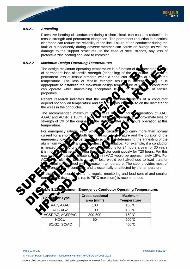
Page 91 of 139 Print Date 4/05/2017
© Horizon Power Corporation – Document Number: HPC-5DC-07-0005-2012
Uncontrolled document when printed. Printed copy expires one week from print date. Refer to Document No. for current version.
8.5.2.1 Annealing Excessive heating of conductors during a short circuit can cause a reduction in tensile strength and permanent elongation. The permanent reduction in electrical clearance can reduce the reliability of the line. Failure of the conductor during the fault or subsequently during adverse weather can cause an outage as well as damage to the support structures. In the case of steel strands, any loss of protective zinc coating can lead to corrosion.
8.5.2.2 Maximum Design Operating Temperatures The design maximum operating temperature is a function of the acceptable level of permanent loss of tensile strength (annealing) of the conductor. There is a permanent loss of tensile strength when a conductor operates at an elevated temperature. The loss of tensile strength results in increased sag. It is appropriate to establish the maximum design temperature at which a conductor can operate while maintaining acceptable levels of degradation of tensile properties.
Recent research indicates that the annealing characteristics of a conductor depend not only on temperature and time of exposure but also on the diameter of the wires in the conductor.
The recommended maximum temperature limit for normal operation of AAC, AAAC and ACSR is 100°C as per AS 7000. This permits an approximate loss of strength of 3% of the original tensile strength after 1000 hours operation at this temperature.
For emergency ratings, (e.g. when one circuit has to carry more than normal current for a short time) both the maximum temperature and the duration of the emergency load should be taken into account in determining the annealing of the aluminium wires. The annealing effect is cumulative. For example, if a conductor is heated to 150°C under emergency conditions for 24 hours a year for 30 years it is much the same as heating the conductor continuously for 720 hours. For this example, the loss of ultimate strength in AAC would be approximately 15%. For ACSR the ultimate tensile strength loss would be halved due to load transfer from aluminium to steel with increase in temperature. The steel provides most of the strength of the conductor and is essentially unaffected by the temperature.
In distribution lines, there is no regular monitoring and load control and smaller temperature rise margins (up to 75°C maximum) is recommended.
Table 8.12 - Maximum Emergency Conductor Operating Temperatures
Conductor Type Cross-sectional area (mm2)
Maximum Temperature
AAC, AAAC 100 160°C ACSR/GZ 100 160°C
ACSR/AZ, ACSR/AC 300-500 150°C HDCU 60 200°C
SC/GZ, SC/AC 400°C
SUPERSEDED 04/0
5/201
7 BY
DISTRIB
UTION D
ESIGN R
ULES
HPC-9DJ-
01-0
002-
2015
Page 92 of 139 Print Date 4/05/2017
© Horizon Power Corporation – Document Number: HPC-5DC-07-0005-2012
Uncontrolled document when printed. Printed copy expires one week from print date. Refer to Document No. for current version.
8.5.2.3 Design Issues a) Sag under fault
Lower maximum temperatures than listed in the Table 12 may be necessary in order to prevent a conductor under fault sagging into equipment below it.
The minimum clearance under fault conditions should be the non flashover distances specified in Table 8-5.
b) Movement of conductors under fault
The movement of conductors due to the electromagnetic forces generated by large short time currents is a complex matter for which a simple satisfactory solution is not available.
c) Structure design
By taking these criteria and the degree of reliability required into account a suitable compromise on structure design, conductor configuration and economics can be achieved.
8.5.3 Sag/Tension Calculations There is a separate ‘Sag tension’ module in the overhead line simulation software program that can be used for calculations for a particular case.
For the bare overhead conductor system, the standard tensions used for standard designs are as follows:
8.5.3.1 Short bays (Urban) In built-up areas, where spans are generally shorter because of residential service requirements, nominal tension of 10% of CBL for AAC conductor and 7% of CBL for AAAC is recommended.
8.5.3.2 Long Spans(Rural) AAC conductor with nominal tension 18% of CBL is recommended for spans in the 60 m to 105 m range in outer urban areas.
AAAC conductor with nominal tension 18% of CBL is recommended for spans in the 60 m to 135 m range in rural areas.
For very long spans up to 250 m in rural areas, SC/GZ or SC/AC conductor with nominal tension 25% of CBL is recommended.
SUPERSEDED 04/0
5/201
7 BY
DISTRIB
UTION D
ESIGN R
ULES
HPC-9DJ-
01-0
002-
2015
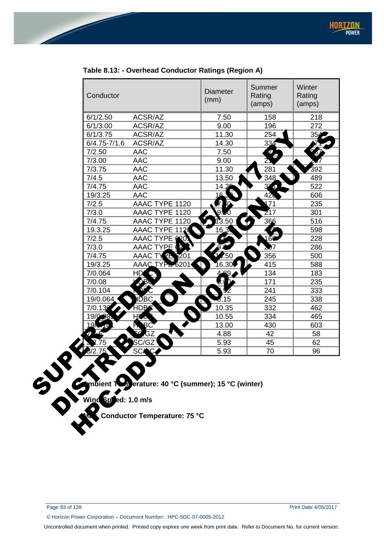
Page 93 of 139 Print Date 4/05/2017
© Horizon Power Corporation – Document Number: HPC-5DC-07-0005-2012
Uncontrolled document when printed. Printed copy expires one week from print date. Refer to Document No. for current version.
Table 8.13: - Overhead Conductor Ratings (Region A)
Conductor Diameter (mm)
Summer Rating (amps)
Winter Rating (amps)
6/1/2.50 ACSR/AZ 7.50 158 218 6/1/3.00 ACSR/AZ 9.00 196 272 6/1/3.75 ACSR/AZ 11.30 254 354 6/4.75-7/1.6 ACSR/AZ 14.30 334 471 7/2.50 AAC 7.50 172 237 7/3.00 AAC 9.00 215 297 7/3.75 AAC 11.30 281 392 7/4.5 AAC 13.50 348 489 7/4.75 AAC 14.25 371 522 19/3.25 AAC 16.30 428 606 7/2.5 AAAC TYPE 1120 7.50 171 235 7/3.0 AAAC TYPE 1120 9.00 217 301 7/4.75 AAAC TYPE 1120 13.50 366 516 19.3.25 AAAC TYPE 1120 16.30 422 598 7/2.5 AAAC TYPE 6201 7.50 166 228 7/3.0 AAAC TYPE 6201 9.00 207 286 7/4.75 AAAC TYPE 6201 13.50 356 500 19/3.25 AAAC TYPE 6201 16.30 415 588 7/0.064 HDBC 4.89 134 183 7/0.08 HDBC 6.00 171 235 7/0.104 HDBC 7.92 241 333 19/0.064 HDBC 8.15 245 338 7/0.136 HDBC 10.35 332 462 19/0.083 HDBC 10.55 334 465 19/0.101 HDBC 13.00 430 603 7/1.6 SC/GZ 4.88 42 58 3/2.75 SC/GZ 5.93 45 62 3/2.75 SC/AC 5.93 70 96
Ambient Temperature: 40 °C (summer); 15 °C (winter)
Wind Speed: 1.0 m/s
Max. Conductor Temperature: 75 °C
SUPERSEDED 04/0
5/201
7 BY
DISTRIB
UTION D
ESIGN R
ULES
HPC-9DJ-
01-0
002-
2015

Page 94 of 139 Print Date 4/05/2017
© Horizon Power Corporation – Document Number: HPC-5DC-07-0005-2012
Uncontrolled document when printed. Printed copy expires one week from print date. Refer to Document No. for current version.
Table 8.14: - Overhead Conductor Ratings (Region C & D)
Conductor Diameter (mm)
Summer Rating (amps)
Winter Rating (amps)
6/1/2.5 ACSR/AZ 7.50 145 177 6/1/3.0 ACSR/AZ 9.00 179 220 6/1/3.75 ACSR/AZ 11.30 230 286 6/4.75-7/1.6 ACSR/AZ 14.30 303 380 7/2.5 AAC 7.50 161 197 7/3.0 AAC 9.00 201 247 7/3.75 AAC 11.30 263 326 7/4.5 AAC 13.50 326 406 7/4.75 AAC 14.30 332 406 19/3.25 AAC 16.30 382 470 7/2.5 AAAC TYPE 1120 7.50 159 194 7/3.0 AAAC TYPE 1120 9.00 198 243 7/4.75 AAAC TYPE 1120 14.30 340 424 19.3.25 AAAC TYPE 1120 16.30 395 497 7/2.5 AAAC TYPE 6201 7.50 151 184 7/3.0 AAAC TYPE 6201 9.00 188 231 7/4.75 AAAC TYPE 6201 14.30 323 403 19/3.25 AAAC TYPE 6201 16.30 376 464 7/0.064 HDBC 4.89 123 148 7/0.08 HDBC 6.00 157 190 7/0.104 HDBC 7.92 220 269 19/0.064 HDBC 8.15 223 273 7/0.136 HDBC 10.35 302 373 19/0.083 HDBC 10.55 304 375 19/0.101 HDBC 13.00 390 486 7/1.60 SC/GZ 4.88 38 46 3/2.75 SC/GZ 5.93 41 50 3/2.75 SC/AC 5.93 62 74
Ambient Temperature: 45 °C (summer); 35 °C (winter)
Wind Speed: 1.0 m/s
Max. Conductor Temperature: 75 °C
SUPERSEDED 04/0
5/201
7 BY
DISTRIB
UTION D
ESIGN R
ULES
HPC-9DJ-
01-0
002-
2015
Page 95 of 139 Print Date 4/05/2017
© Horizon Power Corporation – Document Number: HPC-5DC-07-0005-2012
Uncontrolled document when printed. Printed copy expires one week from print date. Refer to Document No. for current version.
8.6 List of Symbols a distance from lowest point of conductor to lowest support (m)
A cross sectional area of conductor (mm2)
A angle of elevation or depression between supports (degree)
b distance from lowest point of conductor to upper support (m)
d sag of conductor below lowest support (m)
D greater of the two conductor sags at the centre of an equivalent level span and at a conductor operating temperature of 50°C in still air (m)
E Modulus of Elasticity (Pa)
h difference of elevation of supports (m)
hA difference of elevation between supports A and B (m)
hC difference of elevation between supports C and B (m)
K Coefficient of Linear expansion (per °C)
L span length (m)
LT length of conductor (m)
LA length of span between supports A and B (m)
LC length of span between supports C and B (m)
l i length of any freely swinging suspension insulator associated with either conductor (m)
m difference of elevation of conductor at lowest point and at mis-span
S sag at mid-span
SX vertical distance below top support and any point 'X' (m)
T tension in conductor (N)
TA tension in conductor between supports A and B (N)
TC tension in conductor between supports C and B (N)
t1 conductor temperature at initial conditions (°C).
t2 conductor temperature at second set of conditions (°C).
T1 tension at initial conditions (N)
T2 tension at new temperature and/or load per unit length (N)
U r.m.s vector difference in potential between the two conductors when each is ting at its nominal voltage (kV). In determining the potential between conductors of different circuits, regard should be paid to any phase difference in the nominal voltages
W gravitational force on conductor (N/m)
WA gravitational force per unit length on conductor between supports A and B (N/m)
SUPERSEDED 04/0
5/201
7 BY
DISTRIB
UTION D
ESIGN R
ULES
HPC-9DJ-
01-0
002-
2015

Page 96 of 139 Print Date 4/05/2017
© Horizon Power Corporation – Document Number: HPC-5DC-07-0005-2012
Uncontrolled document when printed. Printed copy expires one week from print date. Refer to Document No. for current version.
WC gravitational force per unit length on conductor between supports C and B (N/m)
W1 load on conductor per unit length at initial conditions (N/m)
W2 load on conductor per unit length at standard set of conditions (N/m)
x horizontal distance in span from top support to point 'x' (m)
X Projected horizontal distance between the conductors at mid-span (m)
Y Projected vertical distance between the conductors at mid-span (m)
SUPERSEDED 04/0
5/201
7 BY
DISTRIB
UTION D
ESIGN R
ULES
HPC-9DJ-
01-0
002-
2015
Page 97 of 139 Print Date 4/05/2017
© Horizon Power Corporation – Document Number: HPC-5DC-07-0005-2012
Uncontrolled document when printed. Printed copy expires one week from print date. Refer to Document No. for current version.
9 VOLTAGE REGULATION
9.1 Voltage Tolerance Limits
9.1.1 Statutory Voltage Tolerance Limits Horizon Power declares the voltage level at a customer’s point of supply as within ± 6% of the nominal 240 V single phase and ± 6% of the nominal 415 V three phase.
As such, the maximum and minimum phase-to-neutral voltage levels at any point of supply on the LV network shall be within 225 V and 254 V for single phase supplies and within 390 V and 440 V for three phase supplies (under normal network conditions).
In accordance with AS 61000.3.100 – 2011, Horizon Power expects to adopt the new voltage standard 230 V +6%, -10% for single phase and 400 V +6%, -10% for three phase supplies sometime in the future.
When planning and designing a residential distribution network, the designer has to ensure that the voltages at any point of supply on the network will be within the statutory voltage tolerance limits, under normal network conditions.
9.1.2 Voltage Drop Criteria Impedance in each of the following components of the distribution system leads to voltage drop:
1) Medium Voltage Feeder;
2) Distribution Transformer;
3) Low Voltage Network;
4) Customer Service Leads/Cables.
After a distribution system has been constructed, there are only two locations where voltage levels can be adjusted:
1) at the zone substation (bus-bar voltage set-point and the use of Line Drop Compensators), and
2) at the distribution transformers (off load tap changers).
It is therefore important that the non-adjustable parts of the system be designed adequately to fully utilise the voltage control equipment at these locations to keep the customers’ voltages within the statutory voltage tolerance limits.
Table 9.1: - Voltage Drop Limits with respect to nominal voltage Non-Adjustable System
Components Maximum Voltage Drop Limits
Medium Voltage Feeder 5.0% Distribution Transformer 4.0%
Low Voltage Network 5.0% Customer Service Cable 2.0%
SUPERSEDED 04/0
5/201
7 BY
DISTRIB
UTION D
ESIGN R
ULES
HPC-9DJ-
01-0
002-
2015

Page 98 of 139 Print Date 4/05/2017
© Horizon Power Corporation – Document Number: HPC-5DC-07-0005-2012
Uncontrolled document when printed. Printed copy expires one week from print date. Refer to Document No. for current version.
Thus to compensate for voltage drops caused by components in Table 9.1, the Automatic Voltage Regulator (AVR), Line Drop Compensator (LDC) and distribution transformer taps are set accordingly.
With a 2% voltage drop assumed for customer service cables, “coincident” voltage drops, when taken together with zone substation LDC Buck/Boost and distribution transformer tap options are considered a reasonable balance to achieve a customer’s voltage at the meter panel between ± 6% of the nominal 240 V.
Maintenance and Emergency Voltage Limits are shown in Table 9.2.
9.1.3 Effect of Different Load Cycles The majority of customers in a “typical” area will have similar, “normal” load patterns. Some, however, will have load patterns which vary and in extreme cases could be completely opposite to the “normal” pattern.
These are usually single customer loads. Such loads of relatively small magnitude with respect to the total feeder load (or of relatively large magnitude with respect to the total distribution transformer load) can be catered for by adjusting the tap settings on the transformer supplying the load.
Instances could also arise where a particular MV feeder load profile becomes dominant and “masks” the normal load profile of the remaining feeders on the zone substation. Such a feeder could influence the response of the LDC, to the detriment of the remaining feeders and their individual loads. This problem falls into network load modelling and is not dealt with in this manual.
9.1.4 Voltage Drop Limits for LV Networks One of the voltage drop criteria is that the maximum allowable voltage drop limit for the LV network is 5.0%. This translates to a phase-to-neutral voltage drop of 12 V between the transformer LV terminals and the Point of Supply of any load on the network. This limit, however, applies for normal or steady state conditions.
In general, the network designer shall ensure that the design of the network conforms to the voltage drop limits shown in Table 9.2.
Table 9.2 - Maximum Voltage limits for LV Networks
Condition Voltage Limits (Phase to Neutral) % Volts Max (V) Min (V)
Normal or Steady State ±5.0 12 252 228 Maintenance ±7.0 17 257 223 Emergency ±9.0 22 262 218
When designing the network, maintenance or emergency conditions must also be considered. Interconnection with adjacent networks is necessary to maintain the supply.
SUPERSEDED 04/0
5/201
7 BY
DISTRIB
UTION D
ESIGN R
ULES
HPC-9DJ-
01-0
002-
2015
Page 99 of 139 Print Date 4/05/2017
© Horizon Power Corporation – Document Number: HPC-5DC-07-0005-2012
Uncontrolled document when printed. Printed copy expires one week from print date. Refer to Document No. for current version.
9.1.5 MV Voltage Regulation
9.1.5.1 Design Approach The design approach is generally as follows:
(a) Determine loads for maximum, lightly loaded and maintenance conditions.
(b) For least cost option, check that voltage remains within limits for the various loads.
(c) If voltage goes outside limits try various options.
(d) Compare options to determine optimum solution.
9.1.5.2 Computer Modelling In many instances the line electrical data is entered into a suitable computer program for analysis such as Horizon Power’s Power Factory (Digsilent) program. This calculates the voltage variations for each option. The designer still needs to compare the options.
9.1.5.3 Voltage Control Equipment Some voltage control is built into the standard system equipment as follows:
(a) Distribution Transformers:
Out of service manual tap changes of ±2.5% and ±5%.
(b) Zone Substation Transformers:
Typically ±10%, ±13% or +10 - 20%.
In urban areas it has been standard practice to utilise the above two measures only and choose appropriate conductor sizes and distribution transformer location/quantity to provide satisfactory voltage regulation. These are covered in the Chapter 10 on LV Network Design.
Where longer lines are used it can become uneconomic to increase the conductor size. Additional forms of MV voltage control may become the lowest cost option.
The three options usually considered are as follows:
a) Capacitors -typically used for lines of moderate length
(effective when permanently in service)
b) Reactors - typically used for very long lightly loaded lines
(effective when permanently in service)
c) Regulator - can be used to raise or lower voltage
(output voltage varies to suit load conditions)
SUPERSEDED 04/0
5/201
7 BY
DISTRIB
UTION D
ESIGN R
ULES
HPC-9DJ-
01-0
002-
2015
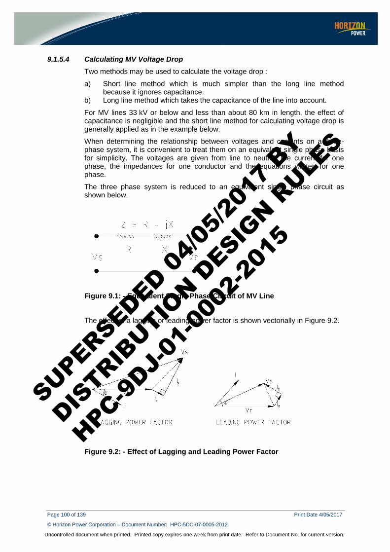
Page 100 of 139 Print Date 4/05/2017
© Horizon Power Corporation – Document Number: HPC-5DC-07-0005-2012
Uncontrolled document when printed. Printed copy expires one week from print date. Refer to Document No. for current version.
9.1.5.4 Calculating MV Voltage Drop Two methods may be used to calculate the voltage drop :
a) Short line method which is much simpler than the long line method because it ignores capacitance.
b) Long line method which takes the capacitance of the line into account.
For MV lines 33 kV or below and less than about 80 km in length, the effect of capacitance is negligible and the short line method for calculating voltage drop is generally applied as in the example below.
When determining the relationship between voltages and currents on a three-phase system, it is convenient to treat them on an equivalent single phase basis for simplicity. The voltages are given from line to neutral, the current for one phase, the impedances for one conductor and the equations written for one phase.
The three phase system is reduced to an equivalent single phase circuit as shown below.
Figure 9.1: - Equivalent Single Phase Circuit of MV Line
The effect of a lagging or leading power factor is shown vectorially in Figure 9.2.
Figure 9.2: - Effect of Lagging and Leading Power Factor
SUPERSEDED 04/0
5/201
7 BY
DISTRIB
UTION D
ESIGN R
ULES
HPC-9DJ-
01-0
002-
2015
Page 101 of 139 Print Date 4/05/2017
© Horizon Power Corporation – Document Number: HPC-5DC-07-0005-2012
Uncontrolled document when printed. Printed copy expires one week from print date. Refer to Document No. for current version.
The symbols used are as follows:
R Resistance in ohms per km (for single conductor);
X Reactance in ohms per km (for single conductor);
Vs Sending end voltage (phase to neutral);
Vr Receiving end voltage (phase to neutral);
I Current in amps per phase;
Φ Phase angle difference between voltage and current vectors
(Power factor = cos Φ)
It is normal operating practice to endeavour to keep the sending end voltage constant and to allow the receiving end voltage to vary according to the load demand.
The receiving end voltage is given approximately by:
𝑽𝑽𝒄𝒄 = 𝑽𝑽𝑺𝑺 − (𝑰𝑰𝑹𝑹 𝐏𝐏𝐜𝐜𝐜𝐜𝚽𝚽 + 𝑰𝑰𝑿𝑿 𝐜𝐜𝐬𝐬𝐬𝐬𝚽𝚽)
The regulation (across the MV line) is given approximately by:
𝑹𝑹𝑺𝑺𝒘𝒘𝑺𝑺𝒊𝒊𝑺𝑺𝑺𝑺𝑺𝑺𝑳𝑳𝑺𝑺 = (𝑽𝑽𝒄𝒄 − 𝑽𝑽𝑺𝑺) ÷ 𝑽𝑽𝑺𝑺𝑳𝑳𝑴𝑴𝑺𝑺𝑺𝑺𝑺𝑺𝒊𝒊 × 𝟏𝟏𝟎𝟎𝟎𝟎%
= (𝑰𝑰𝑹𝑹 𝐏𝐏𝐜𝐜𝐜𝐜𝚽𝚽 + 𝑰𝑰𝑿𝑿 𝐜𝐜𝐬𝐬𝐬𝐬𝚽𝚽) ÷ 𝑽𝑽𝑺𝑺𝑳𝑳𝑴𝑴𝑺𝑺𝑺𝑺𝑺𝑺𝒊𝒊 × 𝟏𝟏𝟎𝟎𝟎𝟎%
9.1.5.5 Worked Example A three phase 22 kV line, 80 km long is required to deliver a load of 630 kVA with a 0.8 p.f. (lagging). The conductor to be used is 7/4.75 AAAC. Determine the regulation of the line
Ip = P ÷ (√3 Vs cos Φ); i.e.
Ip = 630,000 ÷ (√3 × 22,000 × 0.8) = 20.7 A
Resistance per conductor:
RA = 0.3210 Ω/km × 80 km = 25.68 ohm (from conductor manufacturer tables)
Reactance per conductor:
XL = XA + XD
XA = 0.2898 Ω/km (from conductor manufacturer tables)
For a 22 kV country line, the spacing factor (XD) = 0.0857 ohm/km.
Hence, XL = (0.2898 + 0.0857) Ω/km × 80 km = 30.04 ohm.
Receiving end phase voltage:
Vr = Vs - (Ip RA cos Φ + Ip XL sin Φ), i.e.
Vr = 22 ÷ √3 - (20.7 × 25.68 × 0.8 + 20.7 × 30.04 × 0.6) ÷ 1000
i.e. Vr = 11.9 kV (phase to neutral); or
i.e. Vr = √3 × 11.9 = 20.61 kV (phase to phase)
SUPERSEDED 04/0
5/201
7 BY
DISTRIB
UTION D
ESIGN R
ULES
HPC-9DJ-
01-0
002-
2015
Page 102 of 139 Print Date 4/05/2017
© Horizon Power Corporation – Document Number: HPC-5DC-07-0005-2012
Uncontrolled document when printed. Printed copy expires one week from print date. Refer to Document No. for current version.
Hence, the regulation is:
Regulation = (Vs - Vr) ÷ Vnominal × 100%, i.e.
Regulation = (22.0 - 20.90) ÷ 22.0 × 100% = 6.3%
9.2 Line Drop Compensators (LDC) The Automatic Voltage Regulators (AVRs) installed in all zone substations and most voltage regulating transformers are equipped with Line Drop Compensators (LDCs).
LDCs serve to provide a voltage boost at the zone substation busbars in proportion to the load current. For a given MV feeder (modelled as shown in) Figure 9.3, the voltage drop across the feeder’s is proportional to the load current.
If the voltage at the receiving (load) end of the feeder, Vr, is to be maintained at a fixed value, then the voltage at the sending (zone substation) end, Vs must be raised or lowered in proportion to the feeder voltage drop.
The voltage drop across the variable resistor and reactor in the LDC essentially “mimics” the voltage drop in the MV feeder and provides the correct signal to the AVR so that the transformer tap setting can be raised or lowered accordingly.
By suitable adjustment of the LDC’s variable resistor and reactor (which will depend on the outgoing MV feeder’s characteristics), it is possible to obtain constant voltage at some distant point on the feeder, irrespective of the size of the load current or power factor.
Figure 9.3 shows the basic principle behind the LDC
SUPERSEDED 04/0
5/201
7 BY
DISTRIB
UTION D
ESIGN R
ULES
HPC-9DJ-
01-0
002-
2015
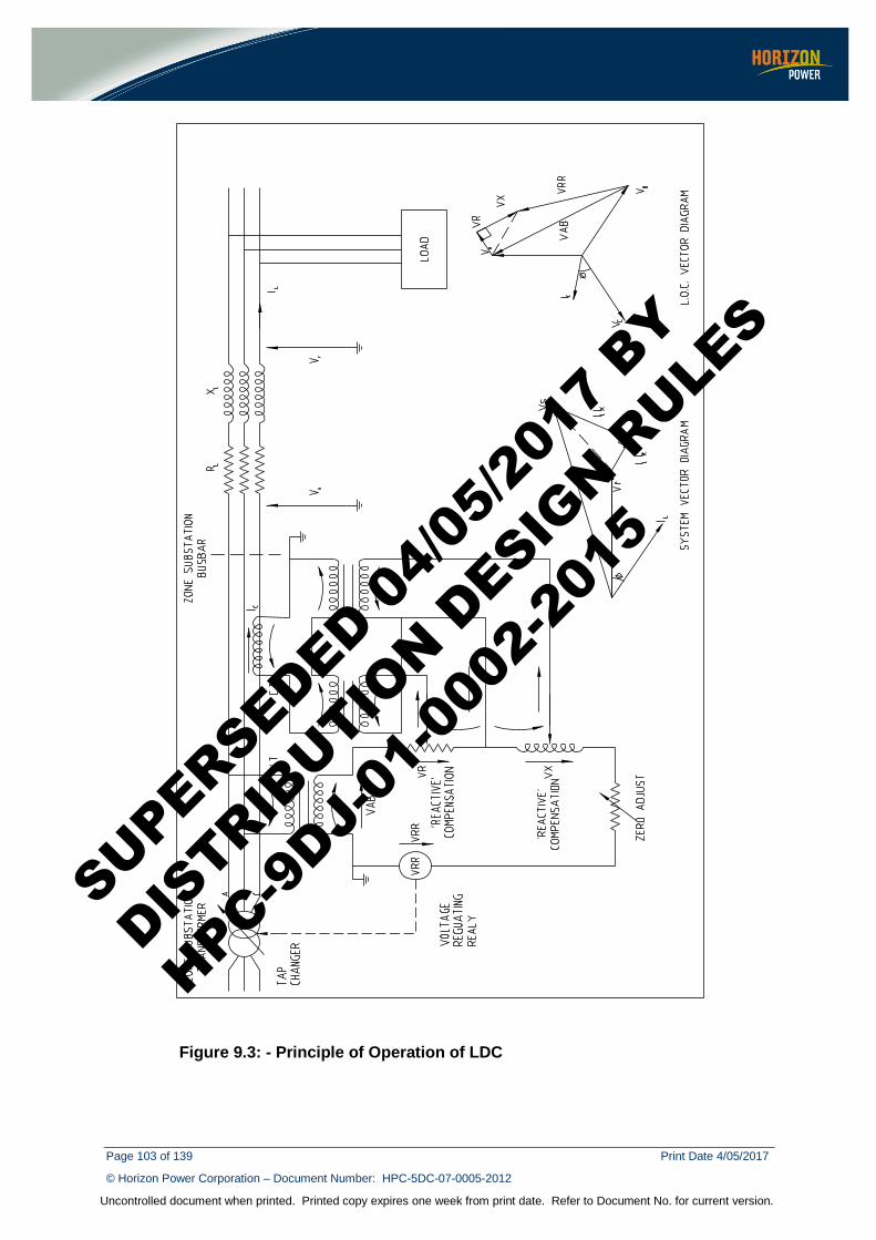
Page 103 of 139 Print Date 4/05/2017
© Horizon Power Corporation – Document Number: HPC-5DC-07-0005-2012
Uncontrolled document when printed. Printed copy expires one week from print date. Refer to Document No. for current version.
Figure 9.3: - Principle of Operation of LDC
SUPERSEDED 04/0
5/201
7 BY
DISTRIB
UTION D
ESIGN R
ULES
HPC-9DJ-
01-0
002-
2015
Page 104 of 139 Print Date 4/05/2017
© Horizon Power Corporation – Document Number: HPC-5DC-07-0005-2012
Uncontrolled document when printed. Printed copy expires one week from print date. Refer to Document No. for current version.
The voltage drops across the LDC’s resistor and reactor are added to the voltage on the output side of the voltage regulating transformer with the correct phasing.
The voltage regulating relay “balances” at one voltage only (the setpoint voltage). The LDC is configured and adjusted so that an increase of load current causes a lowering of the voltage across the voltage regulating relay (VRR). The voltage regulating relay in turn then impulses the tap changer to raise the transformers output voltage until VRR is again equal to the setpoint voltage.
In order to adjust the LDC, the ratio of the main CT and VT as well as the specific feeder impedance must be known. In practice, the settings of the LDC are usually compromise values since most voltage regulating transformers are connected to several outgoing feeders, each with different load characteristics, conductor types, line constructions and line lengths.
The instruction manual pertaining to the particular LDC concerned should be referred to for more detailed information on the operation and adjustment of the LDC.
SUPERSEDED 04/0
5/201
7 BY
DISTRIB
UTION D
ESIGN R
ULES
HPC-9DJ-
01-0
002-
2015
Page 105 of 139 Print Date 4/05/2017
© Horizon Power Corporation – Document Number: HPC-5DC-07-0005-2012
Uncontrolled document when printed. Printed copy expires one week from print date. Refer to Document No. for current version.
10 LV NETWORK DESIGN
10.1 Introduction
10.1.1 General The LV (240/415 V) distribution system is really the “business end” of Horizon Power’s operations. It is the point in Horizon Power’s electricity system where the majority of customers receive their supply.
10.1.2 Primary Aim The primary aim when designing a LV residential distribution network is to ensure that it will adequately service the estimated customer loads both now and in the future. This must be done for the minimum economic cost, while ensuring the network satisfies both reliability and quality of supply standards that are governed by the Electricity Industry (Network Quality and Reliability of Supply) Code 2005.
10.1.3 Challenge for Network Designers The LV network is the most extensive component in the distribution system and accounts for a large proportion of Horizon Power’s capital expenditure. It is also responsible for a large proportion of system losses and customer complaints. Yet it does not always receive the engineering/technical attention it deserves.
The challenge of any residential network designer is to avoid over/under design of the network. Over design is costly in terms of capital investment and is not looked at favourably by the Economic Regulation Authority (ERA). Under design leads to high losses, costly investigation and rectification of Quality of Supply related complaints.
Extra effort expended in optimising the design of LV networks results not only in the efficient utilisation of capital costs but also impacts on the MV network, affecting the number and location of distribution transformers.
10.1.4 Use of Computer Packages Typically, the design studies and calculations are carried out using specially written computer programmes, for the more complex cases or where accurate results are required. Alternatively, manual calculations can sometimes be used, especially for simpler cases or where only estimates are required.
LV DESIGN is a PC based computer program, written specifically for studying LV networks. It is particularly suited for residential estate design, with distributed loads along the LV feeder. The program automatically accounts for load unbalance and diversity.
However, it can also be used to calculate the voltage drops and line currents caused by large commercial loads. LV DESIGN can be used to investigate the impact of new large loads within residential estates, e.g. shopping centres, pumps, etc.
SUPERSEDED 04/0
5/201
7 BY
DISTRIB
UTION D
ESIGN R
ULES
HPC-9DJ-
01-0
002-
2015
Page 106 of 139 Print Date 4/05/2017
© Horizon Power Corporation – Document Number: HPC-5DC-07-0005-2012
Uncontrolled document when printed. Printed copy expires one week from print date. Refer to Document No. for current version.
GIS (Geospatial Information System) is one of Horizon Power's prime computer systems. Various distribution plant items are recorded in the system for most parts of the state, e.g. transformers, MV and LV conductors, poles, and many others. Customer property boundaries are also recorded in the GIS database.
GIS can be used by the designer to obtain information quickly about the existing supply system around a new proposed installation, from which, various supply alternatives can be considered.
GIS can also be used to down-load information on the supply system onto Power Factory (Digsilent) for later analysis.
The electrical and other principles used in the computer packages are briefly outlined in clause 9.1.5.
10.1.5 Aspects of Electrical Design The electrical design of LV distribution feeders generally involves the following aspects:
1) Adherence to voltage tolerance limits;
2) Estimation of load demands;
3) Selection of distribution transformer;
4) Planning of LV network layouts;
5) Calculation of Voltage Drops and Line Currents;
6) Selection of LV conductor sizes to satisfy the voltage drop and line current requirements; and
7) Selection of LV fuse/protection device (if applicable).
These aspects are explained in the following sections.
10.2 Determination of Recommended Load Demand Values
10.2.1 Introduction The current or power flowing from the electricity supply system to an installation at a particular time is known as the electrical demand . Variations of demand occur frequently in domestic installations as individual loads are switched on and off. In a given period, say 24 hours, there will be one value of demand that is higher that all others - this is the maximum demand for that period.
Maximum demand is the all important parameter in system design because this value directly determines component sizes (e.g. conductors, transformers), voltage drops, line currents and ultimately the cost of servicing the loads.
The fluctuating nature of electrical loads, particularly that of residential peaks, makes the measurement of instantaneous demand difficult, and sometimes, undesirable. System components are rated in terms of their thermal (overload) capacity and thus their “average demand ” over a period of, say, 15 minutes is far more meaningful than the moment by moment fluctuations which actually occur. For this reason the demand on electrical equipment is often obtained by the use of special instruments (e.g. load data-loggers) which can provide an average reading for a certain period. The information provided by this type of meter is often employed in system design.
SUPERSEDED 04/0
5/201
7 BY
DISTRIB
UTION D
ESIGN R
ULES
HPC-9DJ-
01-0
002-
2015

Page 107 of 139 Print Date 4/05/2017
© Horizon Power Corporation – Document Number: HPC-5DC-07-0005-2012
Uncontrolled document when printed. Printed copy expires one week from print date. Refer to Document No. for current version.
Subject to predefined conditions, maximum demands can be measured, adjusted and projected to become the basis of design for new systems. While easily understood in principle, maximum demand can be expressed in various terms and measured in various ways. Unless these aspects are fully understood and appreciated, confusion and inaccurate design may result.
The simplest and most common unit of maximum demand is active conductor current, but it is not uncommon to see kVA quoted instead of amps. Other examples include the use of kW (which requires the prevailing power factor to be known), After Diversity Maximum Demand values (ADMD , in kVA), kVA/hectare type figures.
10.2.2 Effect of Load Diversity on Maximum Demand The peak load of any installation is characterised by the demand fluctuations from the switching in and out of appliances within the installation. It is improbable that every appliance will impose its maximum demand at the same instant. As such, the maximum demand of the installation is generally less than the sum of the individual maximum demands of all the appliances within that installation.
Similarly, the maximum demand of a LV feeder is characterised by the demand fluctuations from the varying load demands of all the loads on the feeder. The maximum demand of the feeder will generally be less than the sum of the individual maximum demands due to the “diversity ” between the loads.
It is conceptually possible that if the “average maximum demand” of a “typical” load in a group is known, then the maximum demand for the whole group can be obtained by simply multiplying the average maximum demand of this typical load by the number of loads and also by an appropriate “multiplication factor” chosen for that particular number of loads.
This multiplication factor is commonly referred to as the “diversity factor ”. Used in conjunction with the number of loads, the diversity factor “scales” the “average demand” of a “typical” load within a group, to the maximum demand for that group of loads.
10.2.3 Determination of Design Load Demand Values The maximum demand on a residential substation, when divided by the number of loads supplied, provides a value which is in essence the “average contribution per customer” to that maximum demand, or simply the “average demand” for a “typical” customer. The larger the number of customers involved, the nearer to its ultimate value will be this “average demand”.
For practical purposes, groups of 60 or more loads are considered to produce a figure sufficiently close to the ultimate for it to be considered as the “After Diversity Maximum Demand” or ADMD.
Because the load ADMD is the all important basis of residential distribution design, this matter must receive full and careful consideration, concerning its value at the initial loading of the system, the provision for future growth and the repercussions of having to alter the system as a result of a poor choice of design ADMDs.
SUPERSEDED 04/0
5/201
7 BY
DISTRIB
UTION D
ESIGN R
ULES
HPC-9DJ-
01-0
002-
2015
Page 108 of 139 Print Date 4/05/2017
© Horizon Power Corporation – Document Number: HPC-5DC-07-0005-2012
Uncontrolled document when printed. Printed copy expires one week from print date. Refer to Document No. for current version.
Among the factors influencing the choice of the ultimate design ADMD values are:
1) Limited capital resources;
2) Apprehension concerning the future;
3) Penetration of natural gas in traditionally all-electric areas;
4) Climatic, socio-economic and/or geographic influences;
5) Load growth, changing standard of living;
6) Trend towards more efficient appliances/equipment; and
7) Tariff structure.
Whatever the ultimate design ADMD figures are, the designer must endeavour to ensure that the system is not under/over designed for the reasons given in clause 10.1.3.
Optimum design requires optimum choice of ADMD. In most cases, a designer has to make a value-judgement as to what value of ADMD is most appropriate for the particular distribution system, after having considered all relevant issues.
For most instances, the load demand can be estimated based simply on the designer’s previous experience with similar developments. However, careful thought must still be given to this crucial design parameter for each residential development, rather than simply using highly conservative “standard” values.
It is not uncommon for a designer to find himself/herself in the position of having to be a mixture of an engineer, an economist and even a prophet at the same time!
10.2.4 Application of After Diversity Maximum Demand (ADMD) The after diversity maximum demand (ADMD) electrical loading values must be used when carrying out overhead and underground distribution network design for various customer classes within Horizon Power’s area.
The ADMD values have taken into account seasonal climatic, location and community factors to ensure that adequate capacity is installed for the normal life of Horizon Power’s electrical network assets while ensuring statutory requirements and customer expectations are met in a cost effective manner.
The values of ADMD to be used at a customer level have been based on assessments of load growth patterns experienced in Horizon Power’s regional areas, together Western Australian statutory requirements.
ADMD is the basic electrical load, on a per customer basis, used in the design of Horizon Power’s electrical distribution network. It represents the maximum demand, measured at a distribution substation, where there are more than 60 customers in total connected to that substation.
SUPERSEDED 04/0
5/201
7 BY
DISTRIB
UTION D
ESIGN R
ULES
HPC-9DJ-
01-0
002-
2015
Page 109 of 139 Print Date 4/05/2017
© Horizon Power Corporation – Document Number: HPC-5DC-07-0005-2012
Uncontrolled document when printed. Printed copy expires one week from print date. Refer to Document No. for current version.
10.2.5 Residential Load ADMDs ADMD values for residential loads are provided in Horizon Power document HPC-3DC-07-0001-2012 (Information – Electrical Design for Distribution Networks: After Diversity Maximum Demand). While the ADMD values are applicable only to standard sized lots, there may be cases where the actual ADMDs could be even higher than these values (e.g. for larger lots, beach front houses, riverside lots, canal developments, etc.). Similarly, it may be necessary to reduce the recommended ADMD values. Changes to recommended ADMD values must, at all times, be made in consultation with the technical staff in the relevant Regional Area office prior to the design being carried out.
Since these ADMD values have a sense of “averageness” about them, they must be “scaled up” to obtain the maximum demand for a group of loads before the LV feeder can be designed. The “scaling” of the ADMD values is automatically taken into account in Horizon Power’s Voltage Drop and Line Current formulae.
10.2.6 Non-Residential Load Demands As mentioned earlier, maximum demand values are expressed in a variety of ways, e.g. amps, kVA, kVA/hectare, kW etc. The following load demand values for non-residential loads are a mixture of “average demand” type figures (kVA/hectare figures) as well as “maximum demand” type figures (kVA, kW, hp etc. figures).
Typical design load demand values for non-residential loads are as follows:
1) High Schools: 220 kVA;
2) Primary Schools: 82 kVA;
3) Neighbourhood Shopping Centres: obtain the load kVA based on an average load density of 200 kVA/hectare. (Alternatively, enquire from consultant or measure maximum demand);
4) Large Shops/Business Centres: enquire from consultant;
5) Pumps and other large 3-phase fixed equipment: obtain full load kVA from equipment name-plate or specifications;
6) Small Shop Groups: 200 kVA/hectare;
7) Light Industrial Lots: 100 kVA/hectare.
More information is available in Horizon Power document HPC-5DC-07-003-2012 (Distribution Design Manual Volume 3 – Supply to Large Customer Installations).
10.2.7 Residential Lot Classification Some lots have an “Rn” classification (e.g. R25, R30). This classification relates to the “density” of houses on the lot. The “n” index refers to the Number of Units/hectare, so that an R25 lot classification refers to 25 units per hectare.
Since 1 hectare = 10 000 m2, each unit on a R25 lot would occupy approximately (10 000 ÷ 25) m2 = 400 m2.
The number of units in a given “Rn” lot of area, A (m2), can then be calculated as follows:
SUPERSEDED 04/0
5/201
7 BY
DISTRIB
UTION D
ESIGN R
ULES
HPC-9DJ-
01-0
002-
2015
Page 110 of 139 Print Date 4/05/2017
© Horizon Power Corporation – Document Number: HPC-5DC-07-0005-2012
Uncontrolled document when printed. Printed copy expires one week from print date. Refer to Document No. for current version.
No. of Units = A (m2) × n ÷ 10 000
For example, if an R25 lot has an area of, say, 4898 m2, the number of units in the lot would be 4898 × 25 ÷ 10 000 = 12 units.
10.2.8 LV Conductor Selection Guidelines The size of the LV conductor is chosen to ensure that all of the following criteria are satisfied:
1) Voltage drops during peak network load times being within maximum allowable limits (and during minimum load times being within minimum allowable limits);
2) Conductor current carrying capacity being adequate so that load currents will be within the capacity, not only during steady state conditions, but during maintenance/emergency conditions when the LV network is interconnected with others;
3) Other conductor current ratings (e.g. summer, winter) not being exceeded, wherever applicable;
4) Conductor impedance satisfying the LV fuse/protection requirements (so that at times of fault at the end of the feeder, the fault current will be large enough to be “seen” by the LV fuse and hence, cleared in time to prevent damage to the conductor).
10.2.9 LV Conductor Data Table Horizon Power’s preference is to underground the network as far as possible. However, due to financial considerations and higher capital costs overheads networks will continue to be built. New LV ABC only installations must be constructed using a combination of 95 mm² and 150 mm² LV ABC.
However, LV ABC will also be used to upgrade existing bare overhead systems. Therefore, it is essential that the designer has a table of conductors covering not only LV ABC but other commonly used LV conductors to assist with the design (e.g. when calculating voltage drops, checking current rating violations or checking LV fuse/protection requirements).
10.2.10 Selection of LV Feeder Routes When selecting LV feeder routes, the designer should take the following into account:
10.2.10.1 Proximity to Loads The feeder route should be chosen such that it will “start to be loaded” as close to the transformer as possible. This is facilitated by locating the transformer as close to heavy load centres as possible or as close to the “centre of gravity” of a group of loads.
Feeder routes where the feeder only “picks up” loads after a considerable distance away from the transformer should be avoided (as this causes larger voltage drops than necessary in the initial part of the feeder).
SUPERSEDED 04/0
5/201
7 BY
DISTRIB
UTION D
ESIGN R
ULES
HPC-9DJ-
01-0
002-
2015
Page 111 of 139 Print Date 4/05/2017
© Horizon Power Corporation – Document Number: HPC-5DC-07-0005-2012
Uncontrolled document when printed. Printed copy expires one week from print date. Refer to Document No. for current version.
10.2.10.2 Utilisation/Loading Pole Top Transformers in the overhead system are usually located on “in-line” poles, rather than on “corner poles” to avoid complications during installation, maintenance and operation (switching etc.). At the same time, present policy disallows the running of more than one feeder (or circuit) in parallel (e.g. having two LV circuits on the same bay), unless one or both are ABC.
To overcome this limitation, the designer should ensure that the LV feeder is sufficiently “branched”, i.e. provided with as many “tee-offs” as necessary to service the number of loads.
In general, the LV feeder routes must be chosen such that the transformer will service the required number of loads determined on the basis of design load demand values (refer to clause 10.2.3 and HPC-3DC-07-0001-2012 Electrical Design for Distribution Networks: After Diversity Maximum Demand).
10.2.10.3 Typical Lengths The length of a LV feeder affects the:
1) voltage drop on the feeder; and
2) fault current at the end of the feeder.
Very long LV feeders should generally be avoided since this would only result in higher voltage drops than necessary, cause improper operation and lead to possible conductor burnouts.
10.2.10.4 Interconnection with Other Feeders If a transformer becomes unserviceable, its LV network has to be supplied by adjacent transformers until repairs can be effected or a replacement put into service. As such, the LV network should be provided with sufficient numbers of “interconnecting” points (e.g. via the use of removable solid links, fuse switches) to allow lateral interconnections between LV networks of adjacent transformers.
When selecting LV routes, the designer should select routes which can assist in the provision and location of these “interconnecting points”, if possible.
The interconnection criteria generally used by Horizon Power is to ensure that the backbone feeder of any transformer can be interconnected with other LV feeders from adjacent transformers, at least twice.
If the number of interconnections cannot be provided due to certain constraints, the designer should consider using a smaller transformer size instead.
10.2.10.5 Pole Positioning and Alignment When selecting the LV feeder route, the designer must also give consideration to the positioning of poles adjacent to property boundaries and within the designated pole alignment. Refer to section 4.4 - Pole Position Guidelines.
10.2.10.6 Other Considerations Sometimes, in order to mitigate the excessive voltage drops caused by large motor starting currents, it may be necessary to connect up large motors (e.g.
SUPERSEDED 04/0
5/201
7 BY
DISTRIB
UTION D
ESIGN R
ULES
HPC-9DJ-
01-0
002-
2015
Page 112 of 139 Print Date 4/05/2017
© Horizon Power Corporation – Document Number: HPC-5DC-07-0005-2012
Uncontrolled document when printed. Printed copy expires one week from print date. Refer to Document No. for current version.
large reticulation and sewerage pumps) via a dedicated LV feeder on a separate pole line.
A similar requirement may be called for to mitigate any interferences caused by “potentially disturbing electrical loads” to other customers on the same LV feeder, e.g. light industrial customers with arc-welders, thyristor controlled motor speed drives, large motors.
On the other hand, from the nature of the load itself, or due to special requests from the customer for a more “secure” supply arrangement, certain loads may need to be serviced via dedicated LV feeders or from “sole-use” transformers (e.g. small hospitals, retirement villages, bulk cold food storages).
10.3 Voltage Drops and Line Currents in LV Feeders
10.3.1 General A three phase, four wire distribution system servicing a large proportion of single phase residential loads together with three phase commercial/industrial loads is subject to rapidly fluctuating currents. These currents produce corresponding rapidly fluctuating voltages on the system.
10.3.2 Effect of Load Unbalance It is inevitable that an imbalance between the line currents on the three phases of a feeder will occur if the feeder services a large number of single-phase loads (e.g. residential loads).
This imbalance in the line currents leads to a current which flows in the neutral conductor, which adds to the voltage drop caused by the current flowing in the phase conductor.
The voltage drop calculation (in LV DESIGN software) takes into account this added voltage drop caused by the load unbalance , as necessary.
10.3.3 Voltage Drops/Line Currents in Meshed Networks A “Null Point ” is a point on the meshed portion of the network, through which no line current flows - the voltage drop from the transformer to either side of the null point is also the same.
In practice, the location of the null point in the meshed portion of the network can change as the loads on the meshed portion vary during the day. However, during times of peak load, the location of the null point would be approximately at the same position.
The location of the null point in the meshed portion of the network signifies that the voltage drop from the transformer to either side of the null point is within the maximum allowable limit. Hence, once the location of the null point is known, the network can be assumed to be “opened” at this point and the conductor sizes are appropriate to ensure that the voltage drop to the null point (and hence to all other points on the meshed portion of the network) remains within the maximum allowable limits.
Note: Horizon Power’s Distribution Design Manual - Volume 2 (HPC-5DC-07-0002-2013): Low Voltage Aerial Bundled Cables details the precautions the designer should note when designing with LV ABC to replace existing meshed bare overhead networks.
SUPERSEDED 04/0
5/201
7 BY
DISTRIB
UTION D
ESIGN R
ULES
HPC-9DJ-
01-0
002-
2015
Page 113 of 139 Print Date 4/05/2017
© Horizon Power Corporation – Document Number: HPC-5DC-07-0005-2012
Uncontrolled document when printed. Printed copy expires one week from print date. Refer to Document No. for current version.
SUPERSEDED 04/0
5/201
7 BY
DISTRIB
UTION D
ESIGN R
ULES
HPC-9DJ-
01-0
002-
2015
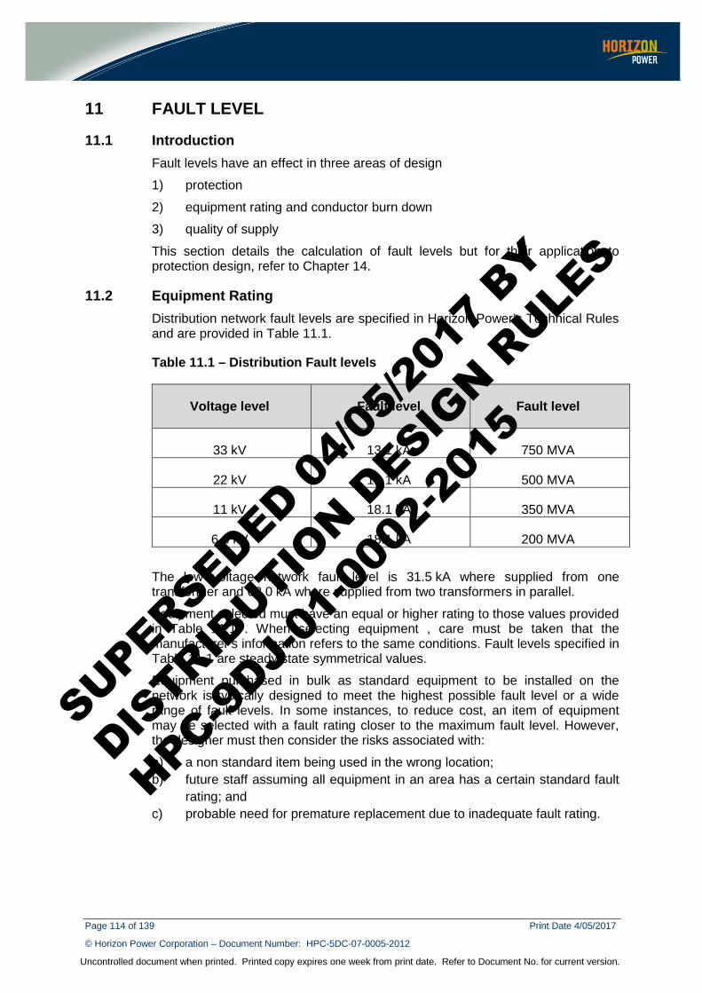
Page 114 of 139 Print Date 4/05/2017
© Horizon Power Corporation – Document Number: HPC-5DC-07-0005-2012
Uncontrolled document when printed. Printed copy expires one week from print date. Refer to Document No. for current version.
11 FAULT LEVEL
11.1 Introduction Fault levels have an effect in three areas of design
1) protection
2) equipment rating and conductor burn down
3) quality of supply
This section details the calculation of fault levels but for their application to protection design, refer to Chapter 14.
11.2 Equipment Rating Distribution network fault levels are specified in Horizon Power’s Technical Rules and are provided in Table 11.1.
Table 11.1 – Distribution Fault levels
Voltage level Fault level Fault level
33 kV 13.1 kA 750 MVA
22 kV 13.1 kA 500 MVA
11 kV 18.1 kA 350 MVA
6.6 kV 18.1 kA 200 MVA
The low voltage network fault level is 31.5 kA where supplied from one transformer and 63.0 kA where supplied from two transformers in parallel.
Equipment selected must have an equal or higher rating to those values provided in Table 11.1 . When selecting equipment , care must be taken that the manufacturer’s information refers to the same conditions. Fault levels specified in Table 11.1 are steady state symmetrical values.
Equipment purchased in bulk as standard equipment to be installed on the network is typically designed to meet the highest possible fault level or a wide range of fault levels. In some instances, to reduce cost, an item of equipment may be selected with a fault rating closer to the maximum fault level. However, the designer must then consider the risks associated with:
a) a non standard item being used in the wrong location; b) future staff assuming all equipment in an area has a certain standard fault
rating; and c) probable need for premature replacement due to inadequate fault rating.
SUPERSEDED 04/0
5/201
7 BY
DISTRIB
UTION D
ESIGN R
ULES
HPC-9DJ-
01-0
002-
2015
Page 115 of 139 Print Date 4/05/2017
© Horizon Power Corporation – Document Number: HPC-5DC-07-0005-2012
Uncontrolled document when printed. Printed copy expires one week from print date. Refer to Document No. for current version.
11.3 Fault Calculation Unless otherwise noted all fault currents are "steady state" symmetrical values.
When calculating maximum fault levels, fault resistance should not normally be included.
When calculating minimum fault levels, a suitable fault resistance should be included.
The following indicates the four main kinds of faults which occur in a power system.
• Three phase fault • Phase to phase fault • Single phase to earth fault • Phase to phase to earth fault
Other fault conditions which may require consideration are short circuits within distribution transformers, conductor open circuits, cross country faults (i.e. simultaneous faults at different points on the system) and system instability.
The magnitude and distribution of fault currents are influenced by the following factors :
a) Source impedance at the zone substation bus bars. b) The arrangement and impedance of the lines, transformers and reactors. c) The neutral earthing arrangements and the value of any neutral earthing
impedance. d) The type of fault and location on the system.
In fault calculations the following simplifying assumptions are often made:
a) The driving voltage remains constant during the fault. (Usually taken as being 100% of nominal system voltage).
b) The effects of load current on the system prior to the fault are ignored as it is small in comparison with the fault currents.
11.4 Formulae Formulae are given below for calculation of the fault level on a per unit basis. The fault level is converted to a current (kA) which is the standard method for specifying equipment fault rating.
Several items of plant which make up the power system will not necessarily all be operating at the same voltage level, it is therefore necessary to express their impedance values in a form which they can be quickly combined directly in the network reduction calculations without reference to the system voltage. The three methods of expressing plant impedances so that they can be directly combined are in:
a) ohms to a common voltage base; b) per cent to a common MVA base; or c) per unit value to a common MVA base
The definition of these quantities is provided in the following sub clauses:
SUPERSEDED 04/0
5/201
7 BY
DISTRIB
UTION D
ESIGN R
ULES
HPC-9DJ-
01-0
002-
2015
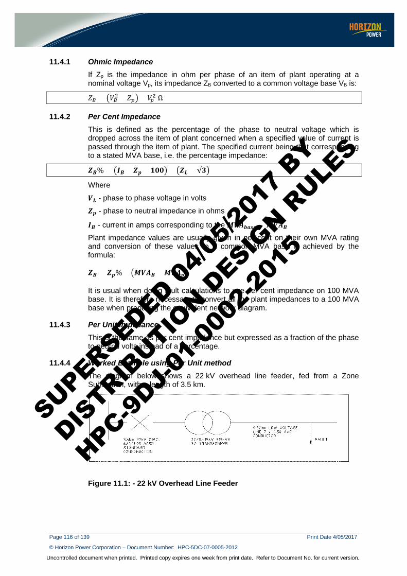
Page 116 of 139 Print Date 4/05/2017
© Horizon Power Corporation – Document Number: HPC-5DC-07-0005-2012
Uncontrolled document when printed. Printed copy expires one week from print date. Refer to Document No. for current version.
11.4.1 Ohmic Impedance If Zp is the impedance in ohm per phase of an item of plant operating at a nominal voltage Vp, its impedance ZB converted to a common voltage base VB is:
𝑍𝑍𝐵𝐵 = 𝑉𝑉𝐵𝐵2 × 𝑍𝑍𝑝𝑝 ÷ 𝑉𝑉𝑝𝑝2 Ω
11.4.2 Per Cent Impedance This is defined as the percentage of the phase to neutral voltage which is dropped across the item of plant concerned when a specified value of current is passed through the item of plant. The specified current being that corresponding to a stated MVA base, i.e. the percentage impedance:
𝒁𝒁𝑩𝑩% = 𝑰𝑰𝑩𝑩 × 𝒁𝒁𝒑𝒑 × 𝟏𝟏𝟎𝟎𝟎𝟎 ÷ 𝒁𝒁𝑳𝑳 ÷ √𝟑𝟑
Where
𝑽𝑽𝑳𝑳 - phase to phase voltage in volts
𝒁𝒁𝒑𝒑 - phase to neutral impedance in ohms
𝑰𝑰𝑩𝑩 - current in amps corresponding to the 𝑴𝑴𝑽𝑽𝑨𝑨𝒃𝒃𝑺𝑺𝑺𝑺𝑺𝑺 = 𝑴𝑴𝑽𝑽𝑨𝑨𝑩𝑩
Plant impedance values are usually given in per cent on their own MVA rating and conversion of these values to a common MVA base is achieved by the formula:
𝒁𝒁𝑩𝑩 = 𝒁𝒁𝒑𝒑% × 𝑴𝑴𝑽𝑽𝑨𝑨𝑩𝑩 ÷ 𝑴𝑴𝑽𝑽𝑨𝑨𝒑𝒑
It is usual when doing fault calculations to use per cent impedance on 100 MVA base. It is therefore necessary to convert all the plant impedances to a 100 MVA base when preparing the equivalent network diagram.
11.4.3 Per Unit Impedance This is the same as per cent impedance but expressed as a fraction of the phase to neutral volts instead of a percentage.
11.4.4 Worked Example using Per Unit method The diagram below shows a 22 kV overhead line feeder, fed from a Zone Substation, with a length of 3.5 km.
Figure 11.1: - 22 kV Overhead Line Feeder
SUPERSEDED 04/0
5/201
7 BY
DISTRIB
UTION D
ESIGN R
ULES
HPC-9DJ-
01-0
002-
2015
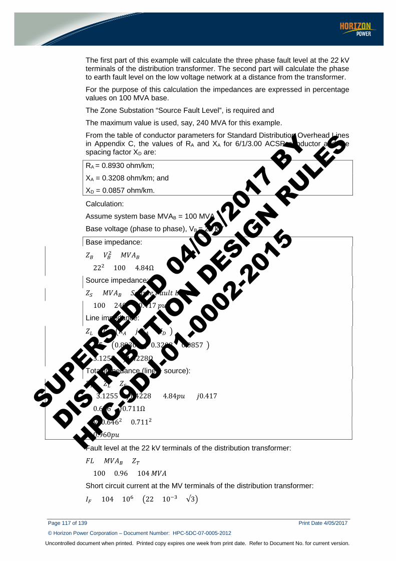
Page 117 of 139 Print Date 4/05/2017
© Horizon Power Corporation – Document Number: HPC-5DC-07-0005-2012
Uncontrolled document when printed. Printed copy expires one week from print date. Refer to Document No. for current version.
The first part of this example will calculate the three phase fault level at the 22 kV terminals of the distribution transformer. The second part will calculate the phase to earth fault level on the low voltage network at a distance from the transformer.
For the purpose of this calculation the impedances are expressed in percentage values on 100 MVA base.
The Zone Substation “Source Fault Level”, is required and
The maximum value is used, say, 240 MVA for this example.
From the table of conductor parameters for Standard Distribution Overhead Lines in Appendix C, the values of RA and XA for 6/1/3.00 ACSR conductor and the spacing factor XD are:
RA = 0.8930 ohm/km;
XA = 0.3208 ohm/km; and
XD = 0.0857 ohm/km.
Calculation:
Assume system base MVAB = 100 MVA
Base voltage (phase to phase), VB = 22 kV
Base impedance:
𝑍𝑍𝐵𝐵 = 𝑉𝑉𝐵𝐵2 ÷ 𝑀𝑀𝑉𝑉𝐴𝐴𝐵𝐵
= 222 ÷ 100 = 4.84Ω
Source impedance:
𝑍𝑍𝑆𝑆 = 𝑀𝑀𝑉𝑉𝐴𝐴𝐵𝐵 ÷ 𝑆𝑆𝐿𝐿𝑀𝑀𝑐𝑐𝑐𝑐𝑝𝑝 𝐹𝐹𝑀𝑀𝑀𝑀𝑝𝑝𝑐𝑐 𝐿𝐿𝑝𝑝𝐿𝐿𝑝𝑝𝑝𝑝
= 100 ÷ 240 = 𝑗𝑗0.417 𝑝𝑝𝑀𝑀
Line impedance:
𝑍𝑍𝐿𝐿 = 𝐿𝐿 × 𝑅𝑅𝐴𝐴 + 𝑗𝑗(𝑋𝑋𝐴𝐴 + 𝑋𝑋𝐷𝐷)
= 3.5 × 0.8930 + 𝑗𝑗(0.3208 + 0.0857)
= 3.1255 + 𝑗𝑗1.4228Ω
Total impedance (line + source):
𝑍𝑍𝑇𝑇 = 𝑍𝑍𝐿𝐿 + 𝑍𝑍𝑆𝑆
= (3.1255 + 𝑗𝑗1.4228) ÷ 4.84𝑝𝑝𝑀𝑀 + (𝑗𝑗0.417)
= 0.646 + 𝑗𝑗0.711Ω
= √(0.6462 + 0.7112)
= 0.960𝑝𝑝𝑀𝑀
Fault level at the 22 kV terminals of the distribution transformer:
𝐹𝐹𝐿𝐿 = 𝑀𝑀𝑉𝑉𝐴𝐴𝐵𝐵 ÷ 𝑍𝑍𝑇𝑇
= 100 ÷ 0.96 = 104 𝑀𝑀𝑉𝑉𝐴𝐴
Short circuit current at the MV terminals of the distribution transformer:
𝐼𝐼𝐹𝐹 = 104 × 106 ÷ 22 × 10−3 × √3
SUPERSEDED 04/0
5/201
7 BY
DISTRIB
UTION D
ESIGN R
ULES
HPC-9DJ-
01-0
002-
2015
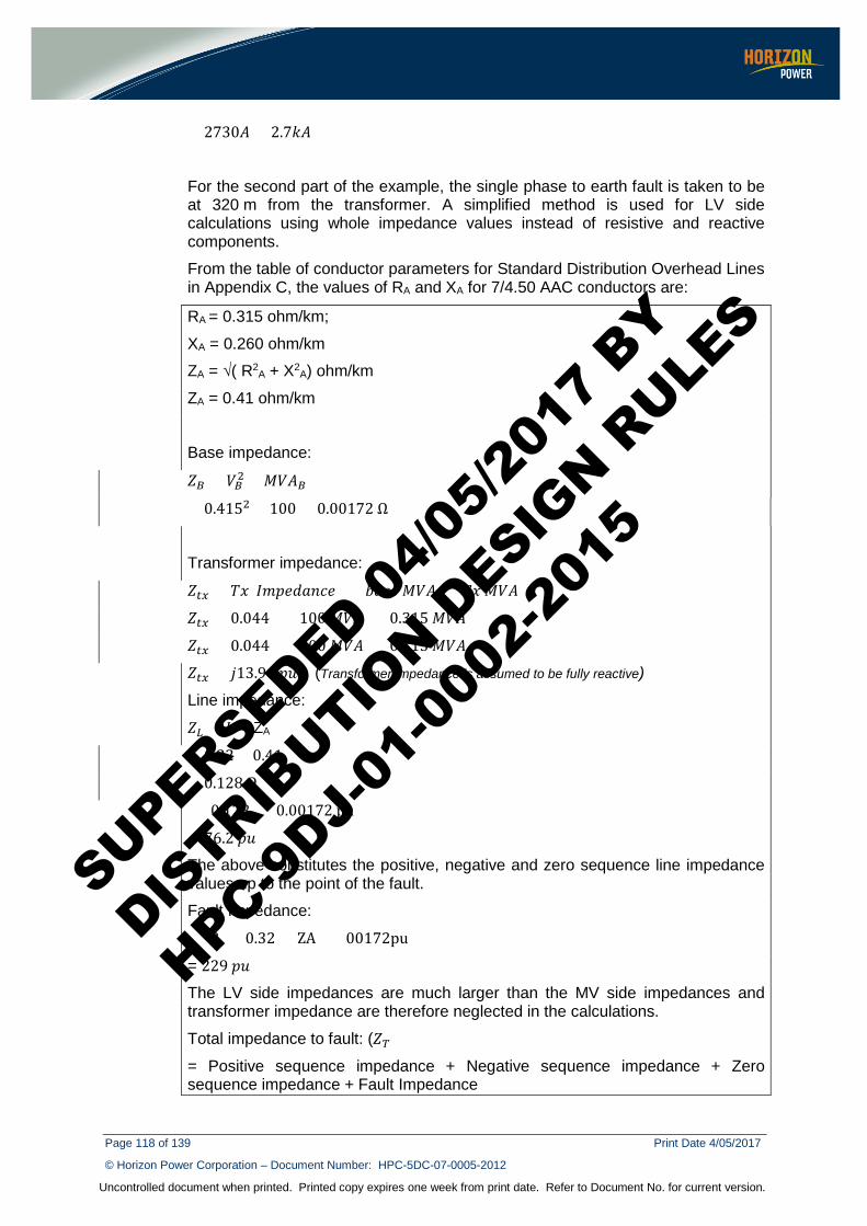
Page 118 of 139 Print Date 4/05/2017
© Horizon Power Corporation – Document Number: HPC-5DC-07-0005-2012
Uncontrolled document when printed. Printed copy expires one week from print date. Refer to Document No. for current version.
= 2730𝐴𝐴 = 2.7𝑘𝑘𝐴𝐴
For the second part of the example, the single phase to earth fault is taken to be at 320 m from the transformer. A simplified method is used for LV side calculations using whole impedance values instead of resistive and reactive components.
From the table of conductor parameters for Standard Distribution Overhead Lines in Appendix C, the values of RA and XA for 7/4.50 AAC conductors are:
RA = 0.315 ohm/km;
XA = 0.260 ohm/km
ZA = √( R2A + X2
A) ohm/km
ZA = 0.41 ohm/km
Base impedance:
𝑍𝑍𝐵𝐵 = 𝑉𝑉𝐵𝐵2 ÷ 𝑀𝑀𝑉𝑉𝐴𝐴𝐵𝐵
= 0.4152 ÷ 100 = 0.00172 Ω
Transformer impedance:
𝑍𝑍𝑡𝑡𝑥𝑥 = 𝑇𝑇𝑀𝑀 𝐼𝐼𝑀𝑀𝑝𝑝𝑝𝑝𝑊𝑊𝑀𝑀𝑊𝑊𝑐𝑐𝑝𝑝 × 𝑏𝑏𝑀𝑀𝑐𝑐𝑝𝑝 𝑀𝑀𝑉𝑉𝐴𝐴 ÷ 𝑇𝑇𝑀𝑀 𝑀𝑀𝑉𝑉𝐴𝐴
𝑍𝑍𝑡𝑡𝑥𝑥 = 0.044 × 100 𝑀𝑀𝑉𝑉𝐴𝐴 ÷ 0.315 𝑀𝑀𝑉𝑉𝐴𝐴
𝑍𝑍𝑡𝑡𝑥𝑥 = 0.044 × 100 𝑀𝑀𝑉𝑉𝐴𝐴 ÷ 0.315 𝑀𝑀𝑉𝑉𝐴𝐴
𝑍𝑍𝑡𝑡𝑥𝑥 = 𝑗𝑗13.96 𝑝𝑝𝑀𝑀 (Transformer impedance is assumed to be fully reactive)
Line impedance:
𝑍𝑍𝐿𝐿 = 𝐿𝐿 × ZA
= 0.32 × 0.41
= 0.128 Ω
= (0.128) ÷ 0.00172 pu
= 76.2 𝑝𝑝𝑀𝑀
The above constitutes the positive, negative and zero sequence line impedance values up to the point of the fault.
Fault Impedance:
= (3 × 0.32 × ZA ) ÷ 00172pu
= 229 𝑝𝑝𝑀𝑀
The LV side impedances are much larger than the MV side impedances and transformer impedance are therefore neglected in the calculations.
Total impedance to fault: (𝑍𝑍𝑇𝑇)
= Positive sequence impedance + Negative sequence impedance + Zero sequence impedance + Fault Impedance
SUPERSEDED 04/0
5/201
7 BY
DISTRIB
UTION D
ESIGN R
ULES
HPC-9DJ-
01-0
002-
2015

Page 119 of 139 Print Date 4/05/2017
© Horizon Power Corporation – Document Number: HPC-5DC-07-0005-2012
Uncontrolled document when printed. Printed copy expires one week from print date. Refer to Document No. for current version.
= (3 X 74.42) + 229 pu
= 457 𝑝𝑝𝑀𝑀
Fault MVA:
𝐹𝐹𝐿𝐿 = 3 × 𝑀𝑀𝑉𝑉𝐴𝐴𝐵𝐵 ÷ 𝑍𝑍𝑇𝑇
= (3 ∗ 100) ÷ 457 = 0.67M𝑉𝑉𝐴𝐴
Fault Current:
= (0.67 ÷ (√3 ∗ 415) = 913 A
11.4.5 Worked example using MVA method The MVA method is a variation to the per unit and ohmic methods.
The example in clause 11.4.4 is reworked in this case. The first step is to convert the typical single line diagram to an equivalent MVA single line diagram and then reduce the MVA single line diagram into a single MVA value at the point of fault.
The equivalent MVA single diagram is provided in Figure 11.2.
22 kV utility source:
= 240 MVA
22 kV Line:
= (222 ÷ 3.43) MVA (√[3.1252 + 1.4232] = 3.43)
= 141 MVA
Fault Level on 22 kV Line:
= 89 MVA (Figure 8.2)
Fault Current:
= (89 ÷ (√3 x 22) A
= 2.4 kA
Transformer:
= 0.315 ÷ 0.044
= 7.2 MVA
LV Line:
= (0.4152 ÷ 0.13) MVA (0.41 x 0.32 = 1.3)
= 1.3 MVA
Fault Impedance:
= (0.4152 ÷ 0.4) MVA (3 x 0.32 x 0.41 = 0.4)
= 0.4 MVA
Fault Level at Fault location
= 3 x 0.2 MVA
= 0.6 MVA
SUPERSEDED 04/0
5/201
7 BY
DISTRIB
UTION D
ESIGN R
ULES
HPC-9DJ-
01-0
002-
2015
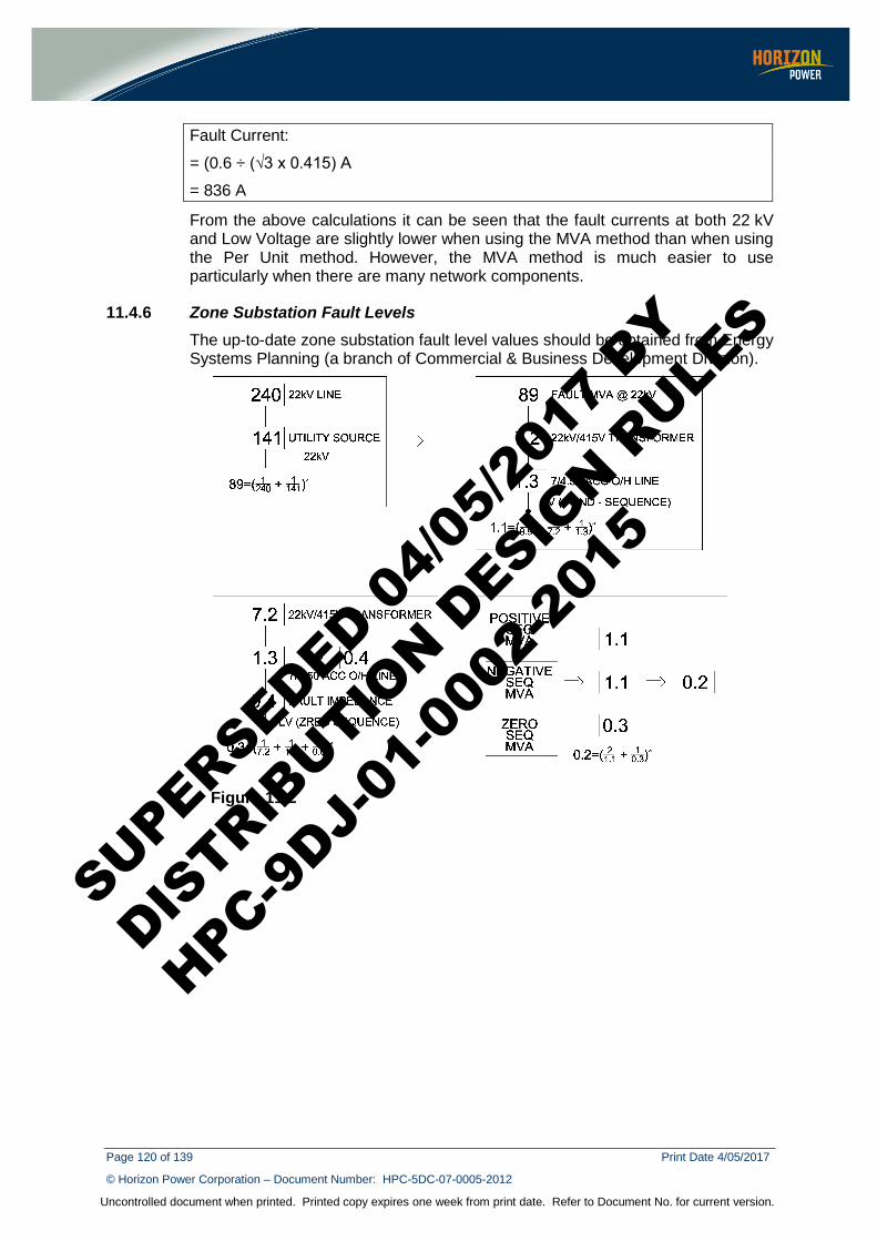
Page 120 of 139 Print Date 4/05/2017
© Horizon Power Corporation – Document Number: HPC-5DC-07-0005-2012
Uncontrolled document when printed. Printed copy expires one week from print date. Refer to Document No. for current version.
Fault Current:
= (0.6 ÷ (√3 x 0.415) A
= 836 A
From the above calculations it can be seen that the fault currents at both 22 kV and Low Voltage are slightly lower when using the MVA method than when using the Per Unit method. However, the MVA method is much easier to use particularly when there are many network components.
11.4.6 Zone Substation Fault Levels The up-to-date zone substation fault level values should be obtained from Energy Systems Planning (a branch of Commercial & Business Development Division).
Figure 11.2
SUPERSEDED 04/0
5/201
7 BY
DISTRIB
UTION D
ESIGN R
ULES
HPC-9DJ-
01-0
002-
2015
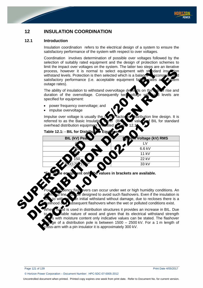
Page 121 of 139 Print Date 4/05/2017
© Horizon Power Corporation – Document Number: HPC-5DC-07-0005-2012
Uncontrolled document when printed. Printed copy expires one week from print date. Refer to Document No. for current version.
12 INSULATION COORDINATION
12.1 Introduction Insulation coordination refers to the electrical design of a system to ensure the satisfactory performance of the system with respect to over voltages.
Coordination involves determination of possible over voltages followed by the selection of suitably rated equipment and the design of protection schemes to limit the impact over voltages on the system. The latter two steps are an iterative process, however it is normal to select equipment with standard insulation withstand levels. Protection is then selected which is a balance of economics and satisfactory performance (i.e. acceptable equipment failure rates and system outage rates).
The ability of insulation to withstand overvoltage depends on the rate of rise and duration of the overvoltage. Consequently two voltage withstand levels are specified for equipment:
• power frequency overvoltage; and • impulse overvoltage
Impulse over voltage is usually the critical factor for distribution line design. It is referred to as the Basic Insulation Level (BIL). The values of BIL for standard overhead distribution equipment are listed in Table 12.1.
Table 12.1: - BIL for Distribution Equipment BIL (kV) Peak System Voltage (kV) RMS
40 LV 60 6.6 kV 95 11 kV 150 22 kV
200(170)(150)* 33 kV
*For some equipment only the values in brackets are available.
Power frequency flashovers can occur under wet or high humidity conditions. An overhead line must be designed to avoid such flashovers. Even if the insulation is able to withstand an initial withstand without damage, due to recloses there is a likelihood of a subsequent flashovers when the wet or polluted conditions exist.
Where wood is used in distribution structures it provides an increase in BIL. Due to the variable nature of wood and given that its electrical withstand strength varies with moisture content only indicative values can be stated. The flashover voltage of a distribution pole is between 1500 – 2500 kV. For a 1 m length of cross-arm with a pin insulator it is approximately 300 kV.
SUPERSEDED 04/0
5/201
7 BY
DISTRIB
UTION D
ESIGN R
ULES
HPC-9DJ-
01-0
002-
2015
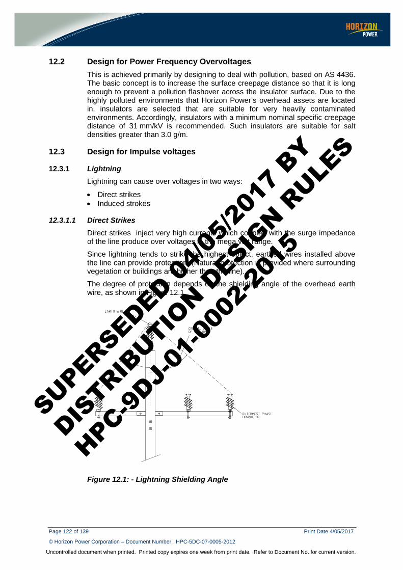
Page 122 of 139 Print Date 4/05/2017
© Horizon Power Corporation – Document Number: HPC-5DC-07-0005-2012
Uncontrolled document when printed. Printed copy expires one week from print date. Refer to Document No. for current version.
12.2 Design for Power Frequency Overvoltages This is achieved primarily by designing to deal with pollution, based on AS 4436. The basic concept is to increase the surface creepage distance so that it is long enough to prevent a pollution flashover across the insulator surface. Due to the highly polluted environments that Horizon Power’s overhead assets are located in, insulators are selected that are suitable for very heavily contaminated environments. Accordingly, insulators with a minimum nominal specific creepage distance of 31 mm/kV is recommended. Such insulators are suitable for salt densities greater than 3.0 g/m.
12.3 Design for Impulse voltages
12.3.1 Lightning Lightning can cause over voltages in two ways:
• Direct strikes • Induced strokes
12.3.1.1 Direct Strikes Direct strikes inject very high currents which coupled with the surge impedance of the line produce over voltages in the mega volt range.
Since lightning tends to strike the highest object, earthed wires installed above the line can provide protection. (Natural protection is provided where surrounding vegetation or buildings are higher than the line).
The degree of protection depends on the shielding angle of the overhead earth wire, as shown in Figure 12.1.
Figure 12.1: - Lightning Shielding Angle
SUPERSEDED 04/0
5/201
7 BY
DISTRIB
UTION D
ESIGN R
ULES
HPC-9DJ-
01-0
002-
2015
Page 123 of 139 Print Date 4/05/2017
© Horizon Power Corporation – Document Number: HPC-5DC-07-0005-2012
Uncontrolled document when printed. Printed copy expires one week from print date. Refer to Document No. for current version.
An angle of 30 degrees has been found to give good protection. On very flat ground this angle could be increased up to 40 degrees.
The average probability of a direct strike to a line can be calculated as follows:
𝑆𝑆𝑐𝑐𝑐𝑐𝑀𝑀𝑘𝑘𝑝𝑝 𝑅𝑅𝑀𝑀𝑐𝑐𝑝𝑝 = 𝑅𝑅𝑐𝑐𝐿𝐿𝑀𝑀𝑊𝑊𝑊𝑊 𝑓𝑓𝑝𝑝𝑀𝑀𝑐𝑐ℎ 𝑊𝑊𝑝𝑝𝑊𝑊𝑐𝑐𝑀𝑀𝑐𝑐𝑎𝑎 × 𝑀𝑀𝑐𝑐𝑝𝑝𝑀𝑀
𝑊𝑊ℎ𝑝𝑝𝑐𝑐𝑝𝑝 𝐴𝐴𝑐𝑐𝑝𝑝𝑀𝑀 = 𝑝𝑝𝑀𝑀𝑊𝑊𝑝𝑝 𝑝𝑝𝑝𝑝𝑊𝑊𝑅𝑅𝑐𝑐ℎ × 𝑝𝑝𝑀𝑀𝑊𝑊𝑝𝑝 ℎ𝑝𝑝𝑀𝑀𝑅𝑅ℎ𝑐𝑐 × 4
For example, 100 km of 9 m high line in an area of ground flash density of 12 flashes/km2/year would have an expected strike rate of
0.2 × 100 × 9 × 4 × 10−3 = 0.72 per year or one every 1.4 years
A map of the Average Annual Number of Thunder Days is shown in Figure 11.2. The relationship between thunder days and ground flash density (Ng) is approximately.
𝑁𝑁𝑟𝑟 = 0.0025𝑇𝑇1.9 flashes per km2/annum
Where, T equals thunder days per annum
SUPERSEDED 04/0
5/201
7 BY
DISTRIB
UTION D
ESIGN R
ULES
HPC-9DJ-
01-0
002-
2015

Page 124 of 139 Print Date 4/05/2017
© Horizon Power Corporation – Document Number: HPC-5DC-07-0005-2012
Uncontrolled document when printed. Printed copy expires one week from print date. Refer to Document No. for current version.
Figure 12.2: - Average Annual Number of Thunder Days SUPERSEDED 0
4/05/2
017
BY
DISTRIB
UTION D
ESIGN R
ULES
HPC-9DJ-
01-0
002-
2015
Page 125 of 139 Print Date 4/05/2017
© Horizon Power Corporation – Document Number: HPC-5DC-07-0005-2012
Uncontrolled document when printed. Printed copy expires one week from print date. Refer to Document No. for current version.
Figure 12.3 – Average Annual lightning ground flash density
SUPERSEDED 0
4/05/2
017
BY
DISTRIB
UTION D
ESIGN R
ULES
HPC-9DJ-
01-0
002-
2015
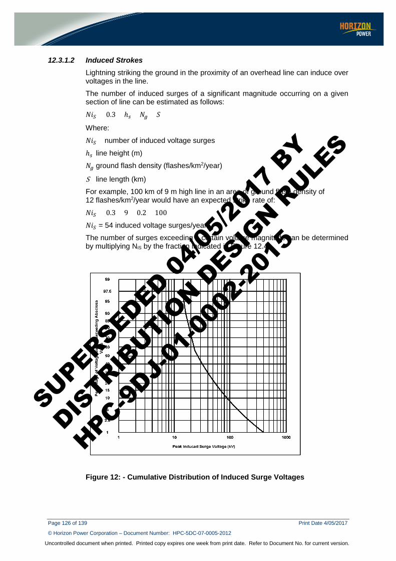
Page 126 of 139 Print Date 4/05/2017
© Horizon Power Corporation – Document Number: HPC-5DC-07-0005-2012
Uncontrolled document when printed. Printed copy expires one week from print date. Refer to Document No. for current version.
12.3.1.2 Induced Strokes Lightning striking the ground in the proximity of an overhead line can induce over voltages in the line.
The number of induced surges of a significant magnitude occurring on a given section of line can be estimated as follows:
𝑁𝑁𝑀𝑀𝑆𝑆 = 0.3 × ℎ𝑐𝑐 ×𝑁𝑁𝑟𝑟 × 𝑆𝑆
Where:
𝑁𝑁𝑀𝑀𝑆𝑆 number of induced voltage surges
ℎ𝑐𝑐 line height (m)
𝑁𝑁𝑟𝑟 ground flash density (flashes/km2/year)
S line length (km)
For example, 100 km of 9 m high line in an area of ground flash density of 12 flashes/km2/year would have an expected strike rate of:
𝑁𝑁𝑀𝑀𝑆𝑆 = 0.3 × 9 × 0.2 × 100
𝑁𝑁𝑀𝑀𝑆𝑆 = 54 induced voltage surges/year
The number of surges exceeding a certain voltage magnitude can be determined by multiplying NiS by the fraction indicated in Figure 12.4.
Figure 12: - Cumulative Distribution of Induced Surge Voltages
SUPERSEDED 04/0
5/201
7 BY
DISTRIB
UTION D
ESIGN R
ULES
HPC-9DJ-
01-0
002-
2015
Page 127 of 139 Print Date 4/05/2017
© Horizon Power Corporation – Document Number: HPC-5DC-07-0005-2012
Uncontrolled document when printed. Printed copy expires one week from print date. Refer to Document No. for current version.
12.3.2 Current Each of the above circumstances induces surges of different magnitude and wave shape. Lightning stroke current usually varies from 3 A to 200 kA, however the average stroke current is 30 kA. The typical lightning flash is usually made up of 3 or 4 strokes, with intervals of 15 to 150 ms between strokes.
12.3.3 Surge Impedance The surge impedance of a 3 phase distribution line is approximately 200 ohms.
An “average” lightning surge of 30 kA would then produce an overvoltage of 6,000 kV.
This is high enough to flashover the full length of a wood pole.
12.3.4 Lightning Protection using Surge Arresters Surge arresters are installed to protect equipment being damaged by lightning. A surge arrester will conduct a surge to ground but will not allow a power frequency flow current to pass.
An arrester’s residual voltage value is the voltage across the arrester whilst it is conducting the surge to ground. The residual voltage needs to be significantly less than the equipment BIL in order to provide satisfactory protection. A “margin of protection” as defined below should be established.
% 𝑀𝑀𝑀𝑀𝑐𝑐𝑅𝑅𝑀𝑀𝑊𝑊 𝐿𝐿𝑓𝑓 𝑃𝑃𝑐𝑐𝐿𝐿𝑐𝑐𝑝𝑝𝑐𝑐𝑐𝑐𝑀𝑀𝐿𝐿𝑊𝑊 (𝑀𝑀𝐿𝐿𝑃𝑃)= (𝐵𝐵𝐼𝐼𝐿𝐿 − 𝑅𝑅𝑝𝑝𝑐𝑐𝑀𝑀𝑊𝑊𝑀𝑀𝑀𝑀𝑝𝑝 𝑉𝑉𝐿𝐿𝑝𝑝𝑐𝑐𝑀𝑀𝑅𝑅𝑝𝑝) ÷ 𝑅𝑅𝑝𝑝𝑐𝑐𝑀𝑀𝑊𝑊𝑀𝑀𝑀𝑀𝑝𝑝 𝑉𝑉𝐿𝐿𝑝𝑝𝑐𝑐𝑀𝑀𝑅𝑅𝑝𝑝 × 100
𝑀𝑀𝐿𝐿𝑃𝑃 = (𝐵𝐵𝐼𝐼𝐿𝐿 − 𝑉𝑉𝑐𝑐𝐿𝐿𝑐𝑐) ÷ 𝑉𝑉𝑐𝑐𝐿𝐿𝑐𝑐 × 100
Where:
BIL - basic insulation level of equipment to be protected (kV)
Vtot - total voltage drop across equipment being protected
12.3.5 Selection of Surge Arresters The steps to be followed are:
1) Select the Rated Voltage for the arrester based on the continuous operating voltage
2) Determine the lightning discharge current. At voltages below 36 kV, 5 kA or 10 kA ratings are specified, however, for Horizon Power’s areas 10 kA is more appropriate.
3) Select the creepage distance (refer to clause 6.1.1)
Surge arrester earth leads must be as short and straight as possible in all surge arrester applications. The primary reason is inductive surge impedance. The selection of an appropriate surge arrester for a given application can be negated by poor installation practices. The length and configuration of the line and earth leads connecting the arrester to the apparatus being protected is critical in the determination of the arrester protective levels and margins.
SUPERSEDED 04/0
5/201
7 BY
DISTRIB
UTION D
ESIGN R
ULES
HPC-9DJ-
01-0
002-
2015
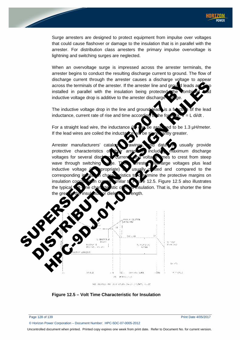
Page 128 of 139 Print Date 4/05/2017
© Horizon Power Corporation – Document Number: HPC-5DC-07-0005-2012
Uncontrolled document when printed. Printed copy expires one week from print date. Refer to Document No. for current version.
Surge arresters are designed to protect equipment from impulse over voltages that could cause flashover or damage to the insulation that is in parallel with the arrester. For distribution class arresters the primary impulse overvoltage is lightning and switching surges are neglected.
When an overvoltage surge is impressed across the arrester terminals, the arrester begins to conduct the resulting discharge current to ground. The flow of discharge current through the arrester causes a discharge voltage to appear across the terminals of the arrester. If the arrester line and ground leads are also installed in parallel with the insulation being protected, the combined lead inductive voltage drop is additive to the arrester discharge voltage.
The inductive voltage drop in the line and ground leads is a function of the lead inductance, current rate of rise and time according to the formula: V = L di/dt .
For a straight lead wire, the inductance (L) can be assumed to be 1.3 µH/meter. If the lead wires are coiled the inductance will be significantly greater.
Arrester manufacturers’ catalogs, drawings, and data will usually provide protective characteristics of their arresters, including maximum discharge voltages for several discharge currents and voltage times to crest from steep wave through switching surge. Those arrester discharge voltages plus lead inductive voltage (if appropriate) are usually plotted and compared to the corresponding insulation characteristics to determine the protective margins on insulation coordination curves similar to Figure 12.5. Figure 12.5 also illustrates the typical volt-time characteristic of most insulation. That is, the shorter the time the greater the insulation or dielectric strength.
Figure 12.5 – Volt Time Characteristic for Insulation
SUPERSEDED 04/0
5/201
7 BY
DISTRIB
UTION D
ESIGN R
ULES
HPC-9DJ-
01-0
002-
2015

Page 129 of 139 Print Date 4/05/2017
© Horizon Power Corporation – Document Number: HPC-5DC-07-0005-2012
Uncontrolled document when printed. Printed copy expires one week from print date. Refer to Document No. for current version.
Published arrester IR discharge voltages are normally based on a standard 8/20 impulse current wave (8 µs to crest and 20 µs to half crest on the tail) however, the highest voltages to which the insulation is subjected are rapidly rising steep wave impulses due to lightning. It is now known that rapidly rising impulse currents are far more common than previously thought. Consistent with this rate of rise, a lead wire voltage drop of 26 kV/m is often used in calculating the protective levels for installations exposed to rapidly rising fast front surges.
The example below illustrates the effect of arrester line and ground leads connected to a surge arrester and connected in parallel with insulation.
Example
The 22 kV transformer in Figure 12.6 needs to be protected from surge damage. The BIL for 22 kV is 150 kV (Table 12.1). The required margin of protection is 50%;
Vtotal = BIL ÷ (MOP) ÷100 + 1
= 150 ÷ 50 ÷100 + 1
= 100 kV
The residual voltage for a suitable arrester with continuous operating voltage 22 kV and rated voltage for a standard 8/20 µs wave is 77 kV (from a manufacturer’s catalogue)
Assuming line and ground lead impedance of 1.3 µH/ft, the resulting inductive voltage developed across the leads = 1.3 x 10‾⁶ x (10 x 103 A / 0.5 x 10‾⁶ sec) = 26 kV/m. (Assuming a 10 kA discharge current cresting at 0.5 µs which is more conservative than a standard 8/20 µs wave) Thus, for every meter length of line and ground lead, 26 kV must be added to the arrester residual voltage when calculating the overvoltage protective margins provided by the arrester and its connections.
If the arrester is not directly connected on to the transformer tank, the ground lead distance ‘d2 ‘ comes into play.
Therefore:
Vtotal = 100 kV = 26 (d1 + d2) + 77
Hence, solving for (d1 + d2):
(d1 + d2) = (100 - 77) ÷ 26
= 0.9 m
The maximum lead distance of (d1 + d2) is 0.9 m in order to provide a margin of protection of 50%.
In this example, if the lead distance is 2.8 m, the MOP is zero, and for higher lead distances the MOP is negative.
SUPERSEDED 04/0
5/201
7 BY
DISTRIB
UTION D
ESIGN R
ULES
HPC-9DJ-
01-0
002-
2015
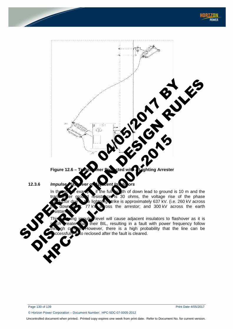
Page 130 of 139 Print Date 4/05/2017
© Horizon Power Corporation – Document Number: HPC-5DC-07-0005-2012
Uncontrolled document when printed. Printed copy expires one week from print date. Refer to Document No. for current version.
Figure 12.6 – Transformer Protected with a Lighting Arrester
12.3.6 Impulse Flashover of Adjacent Insulators In the above example, if the full length of down lead to ground is 10 m and the transformer ground resistance is 30 ohms, the voltage rise of the phase conductor due to the lightning strike is approximately 637 kV. (i.e. 260 kV across the down lead; 77 kV across the arrestor; and 300 kV across the earth resistance).
This lightning impulse level will cause adjacent insulators to flashover as it is much greater than their BIL, resulting in a fault with power frequency follow through current. However, there is a high probability that the line can be successfully auto reclosed after the fault is cleared.
SUPERSEDED 04/0
5/201
7 BY
DISTRIB
UTION D
ESIGN R
ULES
HPC-9DJ-
01-0
002-
2015
Page 131 of 139 Print Date 4/05/2017
© Horizon Power Corporation – Document Number: HPC-5DC-07-0005-2012
Uncontrolled document when printed. Printed copy expires one week from print date. Refer to Document No. for current version.
13 STREET LIGHTING
13.1 Policy Street Lighting is an essential service for the community with importance focused upon safety, security and amenity aspects. As such, Street lighting needs to be provided and maintained to a reasonable standard and with appropriate levels of public accountability.
Effective Street Light operation is best managed through a combination of bulk Street Light replacement, regular night patrols, and response to reports of street light failure from the public in accordance with the published Horizon Power Customer Charter.
13.2 Asset Hierarchy The Street Lighting asset family includes:
• Support structures including steel, wood and concrete poles, outreaches, and foundation etc
• Street Light Control Boxes and its associated accessories and spares • Luminaries: including High Pressure Sodium (HPS), Mercury Vapour
(MV), Metal Halide (MH), Compact Florescent (CFL), Light Emitting Diodes (LED), accessories and spares.
13.3 Lighting Categories and Application The lighting categories are broadly divided as follows:
• Category V lighting: Lighting which is applicable to roads on which the visual requirements of motorists are dominant, e.g. traffic routes. Subcategories range from V1 to V5 (see Table 13.1)
• Category P lighting: Lighting which is applicable to roads on which the visual requirements of pedestrians are dominant, e.g. local roads and to local area traffic management devices (LATMS) installed on such roads. Also lighting which is applicable to outdoor public areas, other than roads, where the visual requirements of pedestrians are dominant, e.g. outdoor shopping precincts. Subcategories range from P1 to P12. Majority of Horizon Power’s street lighting assets fit in category P4. (see Table 13.1)
Table 13.1 indicates the lighting category, typical spacing, pole heights and lamp types used in Horizon Power.
SUPERSEDED 04/0
5/201
7 BY
DISTRIB
UTION D
ESIGN R
ULES
HPC-9DJ-
01-0
002-
2015
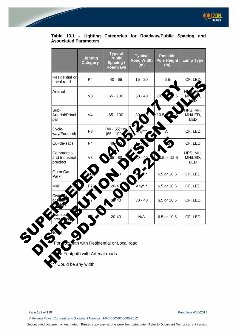
Page 132 of 139 Print Date 4/05/2017
© Horizon Power Corporation – Document Number: HPC-5DC-07-0005-2012
Uncontrolled document when printed. Printed copy expires one week from print date. Refer to Document No. for current version.
Table 13.1 - Lighting Categories for Roadway/Public Spacing and Associated Parameters.
Lighting Category
Type of Public
Spacing / Roadways
Typical Road Width
(m)
Possible Pole Height
(m) Lamp Type
Residential or Local road P4 40 - 65 15 - 20 6.5 CF, LED
Arterial V3 65 - 100 30 - 40 10.5 or 12.5
HPS, MH, MH/LED,
LED
Sub-Arterial/Principal
V4 65 - 100 30 - 40 10.5 or 12.5 HPS, MH, MH/LED,
LED
Cycle-way/Footpath P3 (40 - 65)* or
(65 - 100)** Any*** All CF, LED
Cul-de-sacs P4 40 - 65 15 - 20 6.5 CF, LED
Commercial and Industrial precinct
V3 65 - 80 30 - 40 10.5 or 12.5 HPS, MH, MH/LED,
LED
Open Car Park P11 20-40 Any*** 6.5 or 10.5 CF, LED
Mall P7 20-40 Any*** 6.5 or 10.5 CF, LED
Civic square or Retail precinct
P7 20-40 30 - 40 6.5 or 10.5 CF, LED
Transport Interchange P7 20-40 N/A 6.5 or 10.5 CF, LED
Notes:
* For Footpath with Residential or Local road
** For Footpath with Arterial roads
*** Could be any width
SUPERSEDED 04/0
5/201
7 BY
DISTRIB
UTION D
ESIGN R
ULES
HPC-9DJ-
01-0
002-
2015
Page 133 of 139 Print Date 4/05/2017
© Horizon Power Corporation – Document Number: HPC-5DC-07-0005-2012
Uncontrolled document when printed. Printed copy expires one week from print date. Refer to Document No. for current version.
13.4 Lighting Design Basis Lighting design and luminaires must be in accordance with AS 1158.
13.4.1 Selection of Lamp Types The following factors should influence the selection of luminaires;
1) Energy efficiency ( Lumens/ Watt) 2) Very long life (e.g., 70% light output after 50,000 hours) 3) Very low/ no maintenance ( no lamp replacement) 4) Low life cycle cost 5) Reduction in Greenhouse gas emissions
Horizon Power currently install a combination of Metal Halide, High Pressure Sodium, Compact Fluorescent and LED lamps depending on the application.
The old incandescent lamps are replaced with the above lamps wherever a pole is replaced or other work makes it appropriate to do so.
The Main Roads Department uses low pressure sodium lights to light crosswalks on highways and major roads. Horizon Power do not use these lights for general highway lighting to allow drivers and pedestrians to readily recognise crosswalks by the distinctive light colour.
13.4.2 Luminaire Technical Requirements 1) Minimum life of 20 years. 2) Comply with AS/NZS 1158.6 and AS/NZS 60598. 3) Must be individually Photo Electric (PE) Cell controlled. 4) Luminaire internal control gear including chokes and Photo Electric (PE)
Cells must comply with AS 3771. 5) Interference suppression must be fitted (in accordance with AS/NZS 4051). 6) Minimum IP 55 rating in accordance with AS 60529. 7) High level resistance to vandalism – Minimum IK08 in accordance with
AS/NZS 1158. 8) Luminaires and their control gear internal wiring must be Double Insulted.
13.4.3 Design Considerations Selection of an efficient luminaire is one thing, however, an efficient design has then to be produced
The following factors should be considered in the design:
1) Energy efficiency (Watts/ Linear metre) 2) Very low/no maintenance (Long lumen life, low dirt depreciation, low PE
replacement) 3) How much of over design for lumen depreciation 4) Low life cycle cost 5) Reduction in Greenhouse gas emissions
SUPERSEDED 04/0
5/201
7 BY
DISTRIB
UTION D
ESIGN R
ULES
HPC-9DJ-
01-0
002-
2015
Page 134 of 139 Print Date 4/05/2017
© Horizon Power Corporation – Document Number: HPC-5DC-07-0005-2012
Uncontrolled document when printed. Printed copy expires one week from print date. Refer to Document No. for current version.
13.4.4 Minimum Lighting Performance Requirements Design methods, requirements and application guidance for each of the lighting categories above are given in the AS/NZS 1158 suite of standards. The minimum design requirements are extracted from AS/NZS for P and V categories and presented Table 13.2 and 13.3 below. All design for new lighting schemes shall comply with as a minimum or exceed these requirements.
13.4.5 Lamp Poles Lamp poles currently used by Horizon Power are limited to concrete, steel or suitable mono or blended materials, expected to have a minimum life span of 40 years. Only circular or eight side polygonal poles are used. Some of the critical characteristics of the poles are:
1) Must be suitable to withstand Region D wind conditions 2) Pole tip deflection at ultimate loads must be less than 4% 3) High vandalism rating of IK 08 in accordance with AS 1158 4) Minimum height above ground of 6.5 m, 10.5 m or 12.5 m 5) Should be installed in the 2.7 m alignment or 0.5 m alignments
When installing or replacing luminaires, on existing overhead power lines the existing poles may need to be utilised. When luminaires have been on every second pole and there is an even number of poles, lights will be required on two adjacent poles.
Individual councils may request extra lights or the use of higher wattage lights.
When poles carrying mains on the standard alignment are a long way from the carriageway edge, it is necessary to install additional poles adjacent to the road for the lights.
On standard width Road Verges the street lighting pole should be erected in the “Pole and Tree” allocation area, i.e. 2.7 m from the Property Line. If this position does not allow enough distance between the kerb edge and the street lighting pole to install a foot path, advice should be sought from the local Shire.
SUPERSEDED 04/0
5/201
7 BY
DISTRIB
UTION D
ESIGN R
ULES
HPC-9DJ-
01-0
002-
2015
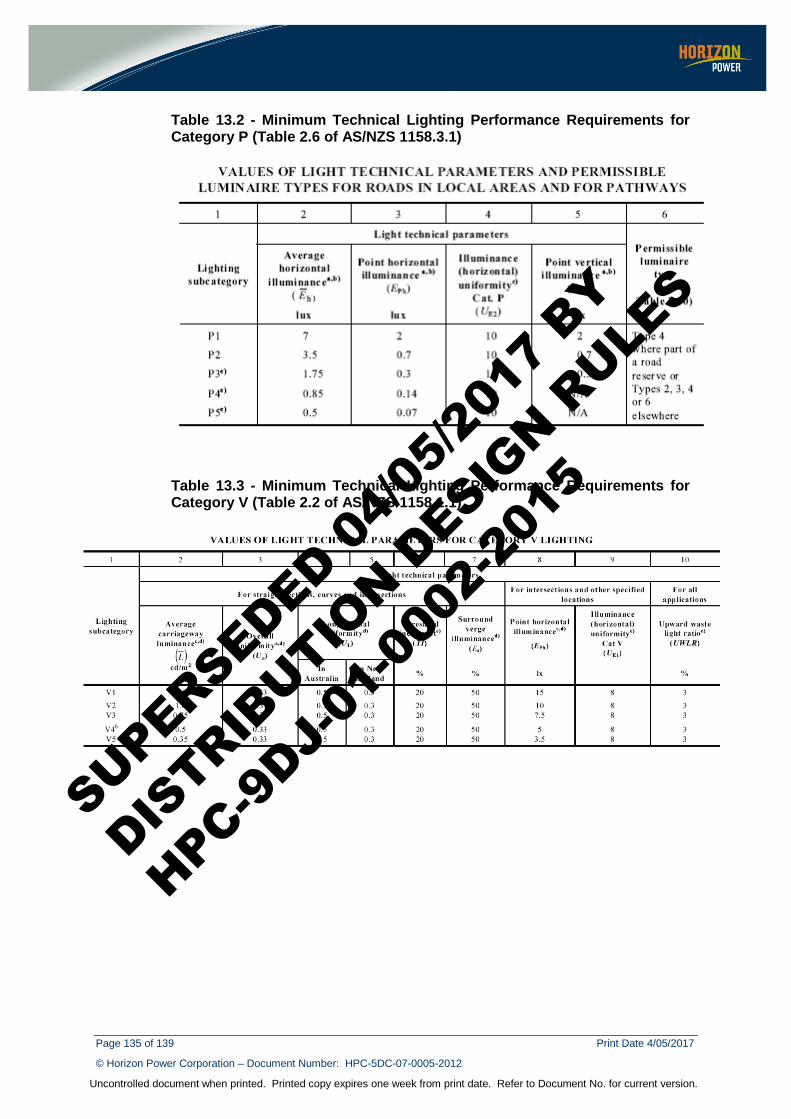
Page 135 of 139 Print Date 4/05/2017
© Horizon Power Corporation – Document Number: HPC-5DC-07-0005-2012
Uncontrolled document when printed. Printed copy expires one week from print date. Refer to Document No. for current version.
Table 13.2 - Minimum Technical Lighting Performance Requirements for Category P (Table 2.6 of AS/NZS 1158.3.1)
Table 13.3 - Minimum Technical Lighting Performance Requirements for Category V (Table 2.2 of AS/NZS 1158.1.1)
SUPERSEDED 04/0
5/201
7 BY
DISTRIB
UTION D
ESIGN R
ULES
HPC-9DJ-
01-0
002-
2015
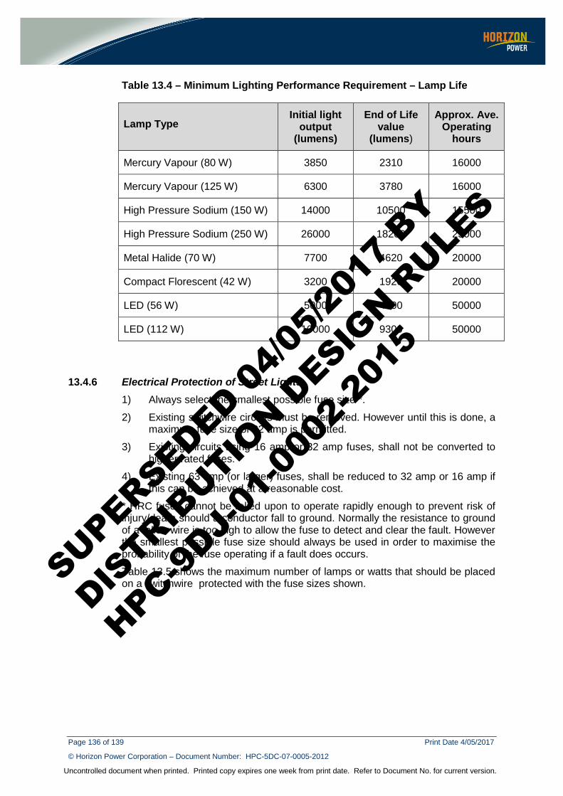
Page 136 of 139 Print Date 4/05/2017
© Horizon Power Corporation – Document Number: HPC-5DC-07-0005-2012
Uncontrolled document when printed. Printed copy expires one week from print date. Refer to Document No. for current version.
Table 13.4 – Minimum Lighting Performance Requirement – Lamp Life
Lamp Type Initial light
output (lumens)
End of Life value
(lumens)
Approx. Ave. Operating
hours
Mercury Vapour (80 W) 3850 2310 16000
Mercury Vapour (125 W) 6300 3780 16000
High Pressure Sodium (150 W) 14000 10500 15500
High Pressure Sodium (250 W) 26000 18200 25000
Metal Halide (70 W) 7700 4620 20000
Compact Florescent (42 W) 3200 1920 20000
LED (56 W) 5000 4600 50000
LED (112 W) 10000 9300 50000
13.4.6 Electrical Protection of Street Lights 1) Always select the smallest possible fuse size *.
2) Existing switchwire circuits must be removed. However until this is done, a maximum fuse size of 32 amp is permitted.
3) Existing circuits using 16 amp or 32 amp fuses, shall not be converted to higher rated fuses.
4) Existing 63 amp (or larger) fuses, shall be reduced to 32 amp or 16 amp if this can be achieved at a reasonable cost.
* HRC fuses cannot be relied upon to operate rapidly enough to prevent risk of injury/death should a conductor fall to ground. Normally the resistance to ground of a fallen wire is too high to allow the fuse to detect and clear the fault. However the smallest possible fuse size should always be used in order to maximise the probability of the fuse operating if a fault does occurs.
Table 13.5 shows the maximum number of lamps or watts that should be placed on a switchwire protected with the fuse sizes shown.
SUPERSEDED 04/0
5/201
7 BY
DISTRIB
UTION D
ESIGN R
ULES
HPC-9DJ-
01-0
002-
2015
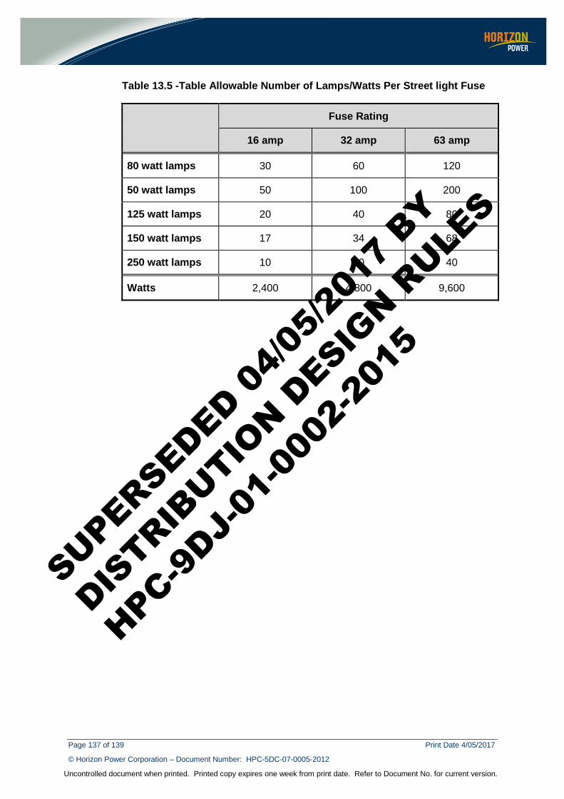
Page 137 of 139 Print Date 4/05/2017
© Horizon Power Corporation – Document Number: HPC-5DC-07-0005-2012
Uncontrolled document when printed. Printed copy expires one week from print date. Refer to Document No. for current version.
Table 13.5 -Table Allowable Number of Lamps/Watts Per Street light Fuse
Fuse Rating
16 amp 32 amp 63 amp
80 watt lamps 30 60 120
50 watt lamps 50 100 200
125 watt lamps 20 40 80
150 watt lamps 17 34 68
250 watt lamps 10 20 40
Watts 2,400 4,800 9,600
SUPERSEDED 04/0
5/201
7 BY
DISTRIB
UTION D
ESIGN R
ULES
HPC-9DJ-
01-0
002-
2015
Page 138 of 139 Print Date 4/05/2017
© Horizon Power Corporation – Document Number: HPC-5DC-07-0005-2012
Uncontrolled document when printed. Printed copy expires one week from print date. Refer to Document No. for current version.
APPENDIX A – REVISION INFORMATION (Informative) Horizon Power has endeavoured to provide standards of the highest quality and would appreciate notification if any errors are found or even queries raised.
Each Standard makes use of its own comment sheet which is maintained throughout the life of the standard, which lists all comments made by stakeholders regarding the standard.
A comment sheet found in DM: 3693210, can be used to record any errors or queries found in or pertaining to this standard, which can then be addressed whenever the standard gets reviewed.
Date Rev No. Notes
01/02/2014 1 First Issue
SUPERSEDED 04/0
5/201
7 BY
DISTRIB
UTION D
ESIGN R
ULES
HPC-9DJ-
01-0
002-
2015
Page 139 of 139 Print Date 4/05/2017
© Horizon Power Corporation – Document Number: HPC-5DC-07-0005-2012
Uncontrolled document when printed. Printed copy expires one week from print date. Refer to Document No. for current version.
APPENDIX B – RELATED INFORMATION This appendix lists other documents that are related to this document
1) Standard – Distribution Design for Power Lines and Cables in the vicinity of Conductive Structures – HPC-9DC-07-0001-2013
2) Standard – Distribution Design for Railway Crossings – HPC-9DC-07-0002-2013 3) Standard – Distribution Design for Water Crossings – HPC-9DC-07-0003-2013 4) Standard – Distribution Line Earthing – HPC-9DC-08-0001-2012 5) Standard – Distribution Electrical Protection – HPC-9DC-19-0001- 2013 6) Information – Essential Distribution Overhead Line Design – HPC-3DC-08-0002-2013
SUPERSEDED 04/0
5/201
7 BY
DISTRIB
UTION D
ESIGN R
ULES
HPC-9DJ-
01-0
002-
2015