Calibration of the New Horizons Long-Range Reconnaissance

Imager

F. Morgan,a S.J. Conard,a H.A. Weaver,a O. Barnouin-Jha,a A.F. Cheng,a H.W. Taylor,a K.A.

Cooper,a R.H. Barkhouser,b R. Boucarut,c E.H. Darlington,a M.P. Grey,a I. Kuznetsov,c T.J.

Madison,c M.A. Quijada,c D.J. Sahnow,b and J.M. Stockd

aJohns Hopkins University Applied Physics Laboratory,

11100 Johns Hopkins Road, Laurel, MD, USA;bJohns Hopkins University, Department of Physics and Astronomy,

3400 N. Charles Street, Baltimore, MD, USA;cNASA Goddard Space Flight Center, MS 551, Greenbelt, MD, USA;

dSwales Aerospace, 5050 Powder Mill Rd., Beltsville, MD, USA

ABSTRACT

The LOng-Range Reconnaissance Imager (LORRI) is a panchromatic imager for the New Horizons Pluto/Kuiperbelt mission. New Horizons is being prepared for launch in January 2006 as the inaugural mission in NASAsNew Frontiers program. This paper discusses the calibration and characterization of LORRI.

LORRI consists of a Ritchey-Chretien telescope and CCD detector. It provides a narrow field of view (0.29◦),high resolution (pixel FOV = 5 µrad) image at f/12.6 with a 20.8 cm diameter primary mirror. The image isacquired with a 1024 × 1024 pixel CCD detector (model CCD 47-20 from E2V). LORRI was calibrated invacuum at three temperatures covering the extremes of its operating range (-100◦C to +40◦C for various partsof the system) and its predicted nominal temperature in-flight. A high pressure xenon arc lamp, selected forits solar-like spectrum, provided the light source for the calibration. The lamp was fiber-optically coupled intothe vacuum chamber and monitored by a calibrated photodiode. Neutral density and bandpass filters controlledsource intensity and provided measurements of the wavelength dependence of LORRI’s performance. This paperwill describe the calibration facility and design, as well as summarize the results on point spread function, flatfield, radiometric response, detector noise, and focus stability over the operating temperature range.

LORRI was designed and fabricated by a combined effort of The Johns Hopkins University Applied PhysicsLaboratory (APL) and SSG Precision Optronics. Calibration was conducted at the Diffraction Grating Evalua-tion Facility at NASA/Goddard Space Flight Center with additional characterization measurements at APL.

Keywords: Pluto, KBO, space, New Horizons, imager

1. INTRODUCTION

The LOng-Range Reconnaissance Imager (LORRI) is a panchromatic imager for NASA’s New Horizons missionto Pluto and the Kuiper belt. The New Horizons spacecraft is currently undergoing testing in preparation forlaunch in January 2006. The spacecraft is expected to fly by Pluto and its moon Charon between 2015 and 2020,depending on launch date, and then continue outward and fly by a Kuiper belt object (KBO). Since the durationof the Pluto/Charon flyby is much shorter than their rotation periods, only one hemisphere of each body will bevisible during close approach. LORRI’s primary mission is to provide detailed images of the opposite hemispheresof Pluto and Charon from relatively great distances during approach to and departure from the system. LORRIwill also support optical navigation and imaging during the Kuiper belt mission.

All of these applications require a sensitive imager with a small field of view and high resolution. LORRIconsists of a Ritchey-Chretien telescope with a backthinned, back-illuminated 1024 × 1024 pixel CCD detector

Further author information: (Send correspondence to F.M.)F.M.: E-mail: frank.morgan@jhuapl.edu, Telephone: 1 240 228 8297

at its focal plane (E2V model 47-20). The telescope operates at f/12.6 with a 20.8 cm aperture and 263 cm focallength. The full field of view is 0.29◦, and the instantaneous FOV (IFOV) is 5 µrad. The LORRI bandpassextends from approximately 350 nm, where the silicon CCD begins to respond, to a short pass filter cutoff atapproximately 900 nm.

This paper discusses the calibration of the LORRI telescope. The calibration facility is described, and anoverview of results for point spread function, flat field, radiometric response, detector noise, and focus stabilityover the operating temperature range is given. Details of the LORRI design, construction and mission arediscussed further in the paper by Conard, et al.1

The objectives of calibration are most easily understood by reference to the calibration equation, whichdescribes the conversion of the signal observed from a scene in instrumental units to the corresponding value inphysical units. In the case of LORRI, the calibration equation can be written

Ix,y,λ =Sx,y,λ,T,t − Biasx,y,T − Darkx,y,T<t − Smearx,y,λ,T,t,φ − Strayx,y,λ,T,t,Φ

FFx,y,λ,T Rλ,T t, (1)

where subscripts x, y denote dependence on detector position (pixel), λ on wavelength, T on temperature, ton exposure time, φ on optical power at other points within the FOV, and Φ on total optical power withinthe telescope. The quantities and their units are I , scene radiance in W m−2 sr−1 nm−1 (see Section 3.5 foran explanation of the spectral units); S, linearized observed signal from scene in DN (for “digital numbers,”increments of the digital output from the CCD readout electronics); Bias, the electronic offset of the CCD signalin DN; Dark, the linearized CCD dark current in DN; Smear, the signal in DN acquired by a pixel as it isshifted through a vertical section of the scene during frame transfer; Stray, the signal due to stray light in DN;FF, flat field response, normalizes to the median of a uniform diffuse source; and R, the absolute responsivity inDNs−1pixel−1/Wm−2sr−1nm−1. (The units given for radiance and responsivity are for diffuse sources; the solidangle drops out of the corresponding quantities for point sources.) Measurement of the terms of the calibrationequation is a primary goal of the calibration. In addition, instrument characteristics such as detector read noise,the imaging point spread function (PSF), and field of view are determined during calibration.

Of the terms in the calibration equation, bias and smear were characterized over the relevant parameters;dark is insignificant at operational temperatures; stray light was tested at discrete off-axis source angles; flatfield response has been measured, but there are difficulties obtaining the desired 0.5% accuracy at all pixelsfrom ground-based data, and in-flight measurements are planned to replace or correct the current flat field;and absolute response has been measured with sufficient accuracy for LORRI science goals. The PSF has beenmeasured at several locations across the FOV, and the field of view and read noise have been determined. Theseevaluations will be described in more detail below.

2. CALIBRATION SETUP

LORRI was calibrated at temperatures spanning its operating temperature range. The telescope assembly tem-perature ranged approximately from -97◦C to -60◦C during calibration, while the CCD temperature ranged from-96◦C to -78◦C. At these low temperatures it was necessary to operate LORRI in vacuum to avoid condensation.The calibration was conducted at the Diffraction Grating Evaluation Facility (DGEF) at Goddard Space FlightCenter, which operates a large vacuum chamber where calibrations of several spaceflight optical instrumentshave been conducted2.

The LORRI calibration was conducted with four principal objectives: to characterize the flat field preciselyfor planetary image analysis, to characterize the point source spatial response for KBO observations and opticalnavigation as well as planetary image analysis, to characterize system parameters such as field of view anddetector bias and noise, and to estimate the approximate absolute response for diffuse and point sources foranalysis flyby configuration planning. Calibrations were conducted in July 2004 prior to environmental testing(vibration, thermal vacuum, etc.) and again in September after environmental testing to establish stabilityof the calibration. The post-environmental calibration was more thorough and provided most of the resultsdiscussed in this paper. To confirm stability of focus and response over the operational temperature range, key

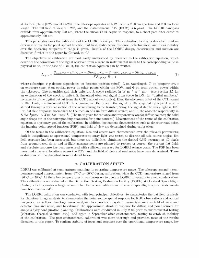
Figure 1. Optical GSE block diagram for the LORRI calibration setup.

measurements were conducted at the nominal temperature as well as temperatures at the upper and lower endsof the operational range.

Figure 1 is a block diagram of the LORRI calibration setup. A light source outside the vacuum chamber wasfiber optically coupled into the chamber, feeding an integrating sphere. The integrating sphere backlit a rotating“target wheel” that contained various apertures such as pinholes and resolution targets. The target wheel was atthe focal plane of a 38 cm diameter collimator, the output of which illuminated LORRI, which was mounted ona two-axis gimbal approximately two meters from the collimator aperture. Between LORRI and the collimator,a 30.5 cm diameter off-axis parabola could be rotated into the beam to focus a pinhole image onto a calibratedphotodiode, providing a measurement of the integrating sphere port radiance for absolute calibration.

The following subsections describe various aspects of the calibration setup in detail.

2.1. Light source

A 150 Watt, high pressure, ozone-free xenon arc lamp was used for the LORRI calibration in order to providea high radiance, solar-like spectrum. Since there are significant spectral variations in response over the LORRIbandpass, it is important to approximate the expected spectral radiance distribution in order to infer broadbandradiometric response from calibration measurements with reasonable accuracy. Sunlight will, of course, providethe illumination for LORRI’s imaging in flight. Although the reflectance spectrum of the observed planetarybodies will modify the spectrum, it will remain at least roughly solar-like.

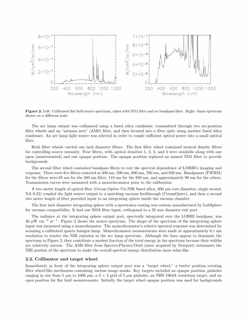
Figure 2. Left: Calibrated flat field source spectrum, taken with ND1 filter and no bandpass filter. Right: Same spectrumshown on a different scale.

The arc lamp output was collimated using a fused silica condenser, transmitted through two six-positionfilter wheels and an “airmass zero” (AM0) filter, and then focused into a fiber optic using another fused silicacondenser. An arc lamp light source was selected in order to couple sufficient optical power into a small opticalfiber.

Both filter wheels carried one inch diameter filters. The first filter wheel contained neutral density filtersfor controlling source intensity. Four filters, with optical densities 1, 2, 3, and 4 were available along with oneopen (unattenuated) and one opaque position. The opaque position replaced an unused ND5 filter to providebackgrounds.

The second filter wheel contained bandpass filters to test the spectral dependence of LORRI’s imaging andresponse. There were five filters centered at 400 nm, 500 nm, 600 nm, 700 nm, and 850 nm. Bandpasses (FWHM)for the filters were 65 nm for the 400 nm filter, 119 nm for the 850 nm, and approximately 90 nm for the others.Transmission curves were measured with a monochromator prior to the calibration.

A two meter length of optical fiber (Ocean Optics Vis-NIR fused silica, 600 µm core diameter, single strand,NA 0.22) coupled the light source output to a matching vacuum feedthrough (CeramOptec), and then a secondtwo meter length of fiber provided input to an integrating sphere inside the vacuum chamber.

The four inch diameter integrating sphere with a spectralon coating was custom manufactured by LabSpherefor vacuum compatibility. It had one SMA fiber input, orthogonal to a 32 mm diameter exit port.

The radiance at the integrating sphere output port, spectrally integrated over the LORRI bandpass, was46 µW cm−2 sr−1. Figure 2 shows the source spectrum. The shape of the spectrum of the integrating sphereinput was measured using a monochomator. The monochromator’s relative spectral response was determined byscanning a calibrated quartz halogen lamp. Monochromator measurements were made at approximately 0.1 nmresolution to resolve the NIR emission in the arc lamp spectrum. Although the lines appear to dominate thespectrum in Figure 2, they contribute a modest fraction of the total energy in the spectrum because their widthsare relatively narrow. The AM0 filter from Spectra-Physics/Oriel (since acquired by Newport) attenuates theNIR portion of the spectrum to make the overall spectral energy distribution more solar-like.

2.2. Collimator and target wheel

Immediately in front of the integrating sphere output port was a “target wheel,” a twelve position rotatingfilter wheel-like mechanism containing various image masks. Key targets included an opaque position, pinholesranging in size from 5 µm to 1000 µm, a 3 × 3 grid of 5 µm pinholes, an NBS 1963A resolution target, and anopen position for flat field measurements. Initially the target wheel opaque position was used for backgrounds

but after experiencing intermittent problems with the target wheel mechanism (which were corrected beforepost-environmental calibration began), the opaque ND filter wheel position was generally used instead.

The target wheel targets were located at the focal plane of a Cassegrain collimator with a 38 cm aperture,460 cm focal length, and 0.5◦ unvignetted field of view. The collimator aperture was large enough to overfillthe LORRI aperture without vignetting over the LORRI FOV and gimbal motion range, with tolerance for easycoalignment. The target wheel was positioned to place the 5 µm pinhole (used for point source characterization)at the collimator focus, determined interferometrically using a spherical reflector in the pinhole position.

2.3. LORRI and gimbal

LORRI was mounted on a two-axis gimbal staring back at the collimator approximately two meters away. Lookingback through the collimator, LORRI viewed the target wheel image masks effectively at infinity. The gimbal(Aerotech model AOM600M) was stepper motor driven with a Unidex controller at 63 steps per arcsecond toscan LORRI across targets. A LORRI pixel subtends roughly one arcsecond.

2.4. Reference photodiode

Between the collimator and LORRI, a 30.5 cm diameter, 152 cm focal length off-axis parabolic mirror on amotorized rotary motion stage could be sent to one of three positions. A “stow” position swung the mirror fullyout of the collimator beam for LORRI observations. A second position focused any of the pinhole targets ontocalibrated photodiode for radiometric reference. A third position moved the pinhole image a few millimeters offof the photodiode for photodiode background determination.

The photodiode was a Hamamatsu S1336-8BQ, with a 5.8 mm square active area. Its responsivity was cali-brated at Hamamatsu at 10 nm intervals from 200 to 400 nm, and at 20 nm intervals from 400 to 1180 nm. Targetpinholes, maximum diameter 1 mm and imaged at 0.33 magnification, were fully captured within the photodiodeactive area. Photodiode current was brought out of vacuum through a BNC feedthrough and measured with aKeithley electrometer.

2.5. Thermal control

LORRI is passively cooled. To control the telescope temperature during calibration, a shroud surrounding thetelescope was liquid nitrogen-cooled. A small annular shroud encircling the telescope inside the cold shroudwas heated to control the telescope temperature to the desired setpoint. This method was found to be morestable than controlling the cold shroud temperature directly with controlled cold gas circulation. The thermalconductivity of the telescope structure was sufficient to guarantee a uniform temperature distribution despitethe uneven heating. The shrouds were fixed, with LORRI gimbaled inside them. LORRI viewed the collimatorthrough a ten inch aperture in the main cold shroud, which kept the shroud edge well out of the LORRI FOVover the maximum gimbal motion range used. A separate, smaller cold shroud and heater similarly controlledthe temperature of the CCD radiator, so the CCD temperature was controlled somewhat independently ofthe telescope structure temperature. The focal plane electronics board was mounted on the baseplate whichsupported the LORRI assembly. The baseplate was heated to control the board temperature.

Table 1 lists the temperatures targeted for the nominal, warm, and cold cases, for the CCD, the CCD readoutelectronics board, and the primary (M1) and secondary (M2) telescope mirrors.

2.6. Command and data

The calibration was controlled by three networked computers. One PC running the Ground Support EquipmentOperating System (GSEOS) commanded LORRI, controlling configuration (exposure time and bin mode) andimage acquisition. A linux PC hosted a frame grabber to acquire and store LORRI images. A second linux PCacted as the master controller and ran IDL scripts that commanded the calibration GSE mechanisms (gimbal,OAP, target wheel, and filter wheels), cued LORRI commands through the GSEOS PC, and cued LORRI imageacquisition through the frame grabber PC.

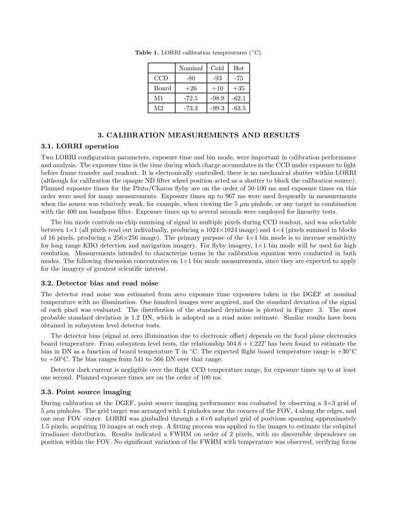
Table 1. LORRI calibration temperatures (◦C).

Nominal Cold Hot

CCD -80 -93 -75

Board +26 +10 +35

M1 -72.5 -98.9 -62.1

M2 -73.3 -99.3 -63.5

3. CALIBRATION MEASUREMENTS AND RESULTS

3.1. LORRI operation

Two LORRI configuration parameters, exposure time and bin mode, were important in calibration performanceand analysis. The exposure time is the time during which charge accumulates in the CCD under exposure to lightbefore frame transfer and readout. It is electronically controlled; there is no mechanical shutter within LORRI(although for calibration the opaque ND filter wheel position acted as a shutter to block the calibration source).Planned exposure times for the Pluto/Charon flyby are on the order of 50-100 ms and exposure times on thisorder were used for many measurements. Exposure times up to 967 ms were used frequently in measurementswhen the source was relatively weak, for example, when viewing the 5 µm pinhole, or any target in combinationwith the 400 nm bandpass filter. Exposure times up to several seconds were employed for linearity tests.

The bin mode controls on-chip summing of signal in multiple pixels during CCD readout, and was selectablebetween 1×1 (all pixels read out individually, producing a 1024×1024 image) and 4×4 (pixels summed in blocksof 16 pixels, producing a 256×256 image). The primary purpose of the 4×4 bin mode is to increase sensitivityfor long range KBO detection and navigation imagery. For flyby imagery, 1×1 bin mode will be used for highresolution. Measurements intended to characterize terms in the calibration equation were conducted in bothmodes. The following discussion concentrates on 1×1 bin mode measurements, since they are expected to applyfor the imagery of greatest scientific interest.

3.2. Detector bias and read noise

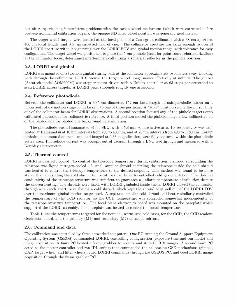
The detector read noise was estimated from zero exposure time exposures taken in the DGEF at nominaltemperature with no illumination. One hundred images were acquired, and the standard deviation of the signalof each pixel was evaluated. The distribution of the standard deviations is plotted in Figure 3. The mostprobable standard deviation is 1.2 DN, which is adopted as a read noise estimate. Similar results have beenobtained in subsystem level detector tests.

The detector bias (signal at zero illumination due to electronic offset) depends on the focal plane electronicsboard temperature. From subsystem level tests, the relationship 504.6 + 1.22T has been found to estimate thebias in DN as a function of board temperature T in ◦C. The expected flight board temperature range is +30◦Cto +50◦C. The bias ranges from 541 to 566 DN over that range.

Detector dark current is negligible over the flight CCD temperature range, for exposure times up to at leastone second. Planned exposure times are on the order of 100 ms.

3.3. Point source imaging

During calibration at the DGEF, point source imaging performance was evaluated by observing a 3×3 grid of5 µm pinholes. The grid target was arranged with 4 pinholes near the corners of the FOV, 4 along the edges, andone near FOV center. LORRI was gimballed through a 6×6 subpixel grid of positions spanning approximately1.5 pixels, acquiring 10 images at each step. A fitting process was applied to the images to estimate the subpixelirradiance distribution. Results indicated a FWHM on order of 2 pixels, with no discernible dependence onposition within the FOV. No significant variation of the FWHM with temperature was observed, verifying focus

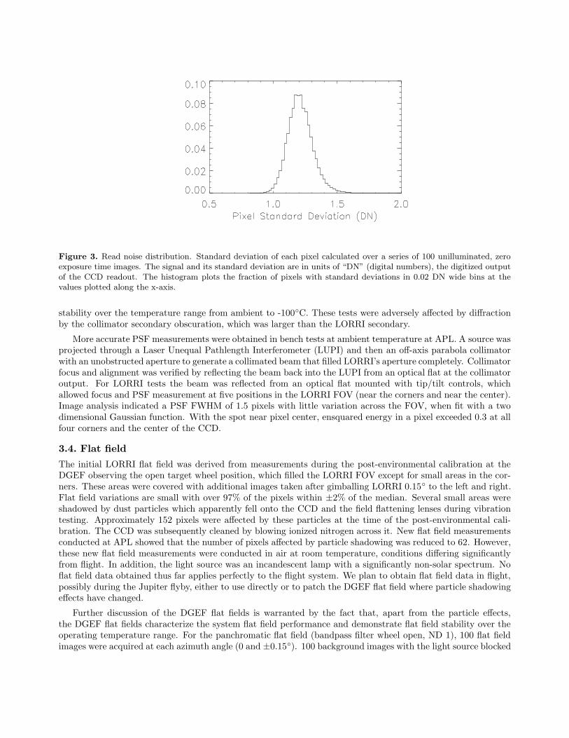
Figure 3. Read noise distribution. Standard deviation of each pixel calculated over a series of 100 unilluminated, zeroexposure time images. The signal and its standard deviation are in units of “DN” (digital numbers), the digitized outputof the CCD readout. The histogram plots the fraction of pixels with standard deviations in 0.02 DN wide bins at thevalues plotted along the x-axis.

stability over the temperature range from ambient to -100◦C. These tests were adversely affected by diffractionby the collimator secondary obscuration, which was larger than the LORRI secondary.

More accurate PSF measurements were obtained in bench tests at ambient temperature at APL. A source wasprojected through a Laser Unequal Pathlength Interferometer (LUPI) and then an off-axis parabola collimatorwith an unobstructed aperture to generate a collimated beam that filled LORRI’s aperture completely. Collimatorfocus and alignment was verified by reflecting the beam back into the LUPI from an optical flat at the collimatoroutput. For LORRI tests the beam was reflected from an optical flat mounted with tip/tilt controls, whichallowed focus and PSF measurement at five positions in the LORRI FOV (near the corners and near the center).Image analysis indicated a PSF FWHM of 1.5 pixels with little variation across the FOV, when fit with a twodimensional Gaussian function. With the spot near pixel center, ensquared energy in a pixel exceeded 0.3 at allfour corners and the center of the CCD.

3.4. Flat field

The initial LORRI flat field was derived from measurements during the post-environmental calibration at theDGEF observing the open target wheel position, which filled the LORRI FOV except for small areas in the cor-ners. These areas were covered with additional images taken after gimballing LORRI 0.15◦ to the left and right.Flat field variations are small with over 97% of the pixels within ±2% of the median. Several small areas wereshadowed by dust particles which apparently fell onto the CCD and the field flattening lenses during vibrationtesting. Approximately 152 pixels were affected by these particles at the time of the post-environmental cali-bration. The CCD was subsequently cleaned by blowing ionized nitrogen across it. New flat field measurementsconducted at APL showed that the number of pixels affected by particle shadowing was reduced to 62. However,these new flat field measurements were conducted in air at room temperature, conditions differing significantlyfrom flight. In addition, the light source was an incandescent lamp with a significantly non-solar spectrum. Noflat field data obtained thus far applies perfectly to the flight system. We plan to obtain flat field data in flight,possibly during the Jupiter flyby, either to use directly or to patch the DGEF flat field where particle shadowingeffects have changed.

Further discussion of the DGEF flat fields is warranted by the fact that, apart from the particle effects,the DGEF flat fields characterize the system flat field performance and demonstrate flat field stability over theoperating temperature range. For the panchromatic flat field (bandpass filter wheel open, ND 1), 100 flat fieldimages were acquired at each azimuth angle (0 and ±0.15◦). 100 background images with the light source blocked

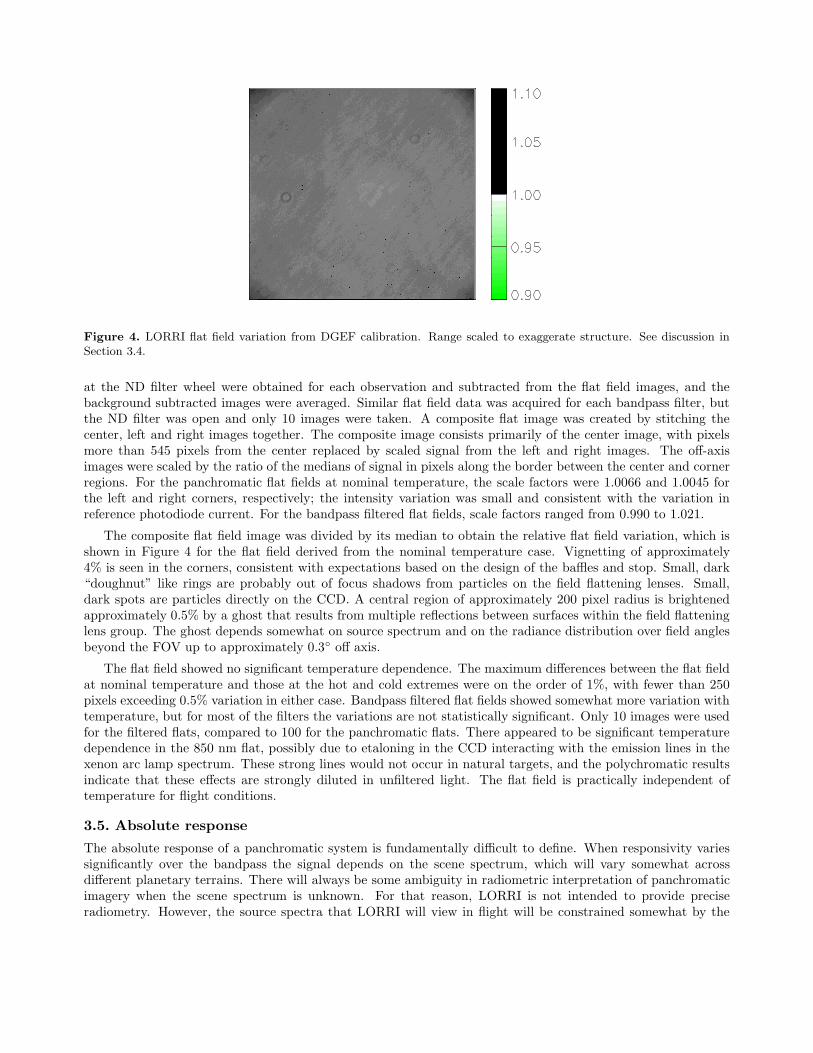
Figure 4. LORRI flat field variation from DGEF calibration. Range scaled to exaggerate structure. See discussion inSection 3.4.

at the ND filter wheel were obtained for each observation and subtracted from the flat field images, and thebackground subtracted images were averaged. Similar flat field data was acquired for each bandpass filter, butthe ND filter was open and only 10 images were taken. A composite flat image was created by stitching thecenter, left and right images together. The composite image consists primarily of the center image, with pixelsmore than 545 pixels from the center replaced by scaled signal from the left and right images. The off-axisimages were scaled by the ratio of the medians of signal in pixels along the border between the center and cornerregions. For the panchromatic flat fields at nominal temperature, the scale factors were 1.0066 and 1.0045 forthe left and right corners, respectively; the intensity variation was small and consistent with the variation inreference photodiode current. For the bandpass filtered flat fields, scale factors ranged from 0.990 to 1.021.

The composite flat field image was divided by its median to obtain the relative flat field variation, which isshown in Figure 4 for the flat field derived from the nominal temperature case. Vignetting of approximately4% is seen in the corners, consistent with expectations based on the design of the baffles and stop. Small, dark“doughnut” like rings are probably out of focus shadows from particles on the field flattening lenses. Small,dark spots are particles directly on the CCD. A central region of approximately 200 pixel radius is brightenedapproximately 0.5% by a ghost that results from multiple reflections between surfaces within the field flatteninglens group. The ghost depends somewhat on source spectrum and on the radiance distribution over field anglesbeyond the FOV up to approximately 0.3◦ off axis.

The flat field showed no significant temperature dependence. The maximum differences between the flat fieldat nominal temperature and those at the hot and cold extremes were on the order of 1%, with fewer than 250pixels exceeding 0.5% variation in either case. Bandpass filtered flat fields showed somewhat more variation withtemperature, but for most of the filters the variations are not statistically significant. Only 10 images were usedfor the filtered flats, compared to 100 for the panchromatic flats. There appeared to be significant temperaturedependence in the 850 nm flat, possibly due to etaloning in the CCD interacting with the emission lines in thexenon arc lamp spectrum. These strong lines would not occur in natural targets, and the polychromatic resultsindicate that these effects are strongly diluted in unfiltered light. The flat field is practically independent oftemperature for flight conditions.

3.5. Absolute response

The absolute response of a panchromatic system is fundamentally difficult to define. When responsivity variessignificantly over the bandpass the signal depends on the scene spectrum, which will vary somewhat acrossdifferent planetary terrains. There will always be some ambiguity in radiometric interpretation of panchromaticimagery when the scene spectrum is unknown. For that reason, LORRI is not intended to provide preciseradiometry. However, the source spectra that LORRI will view in flight will be constrained somewhat by the

fixed spectrum of the illuminating source (the sun), modified by variable surface albedos. LORRI may providesome useful radiometric data as long as the range of uncertainty due to unknown source spectrum can beestimated. It is also important for observation planning to establish the approximate absolute response, so thatexposure times can be set to provide reasonable signals, for example.

In order to determine the dependence of LORRI response on scene spectrum, it was necessary to estimateLORRI’s absolute responsivity as a function of wavelength. This was done using panchromatic absolute measure-ments together with a calculated relative response curve. First, the LORRI responsivity spectrum was calculatedfrom geometrical throughput considerations and estimates of subsystem spectral performance. It was assumedthat this curve approximated the shape of the LORRI response spectrum, and that an unknown constant factorwould scale it to the correct absolute level. Second, the LORRI response spectrum was determined using

Rλ,T = ρλ

[

ST

(

D2

L − B2

L

)

(D2

L − B2

C)∫

Iλ(λ)ρλ(λ)dλ

]

, (2)

where DL is the LORRI aperture diameter, BL and BC are the effective obscuration diameters of the secondaryand spider of LORRI and the collimator, respectively, ST is the LORRI calibration signal at temperature after flatfield correction, Iλ is the calibrated source spectral radiance (Figure 2), and ρλ is the calculated LORRI responsecurve. The quantity in square brackets scales the calculated relative response curve ρλ to the absolute responserequired to fit the observed calibration signal S. The ratio of geometric terms corrects for signal reductionfrom the partial blockage of LORRI’s aperture by the collimator secondary, which is larger than LORRI’ssecondary. Lastly, the response to a range of realistic scene spectra was calculated numerically by integratingthe product of the assumed scene spectra and the LORRI response spectrum derived from calibration. Bandpassfilter response measurements confirm that the shape of the main portion of the LORRI response spectrum isreasonably approximated by the calculated curve. These steps are described more fully as follows.

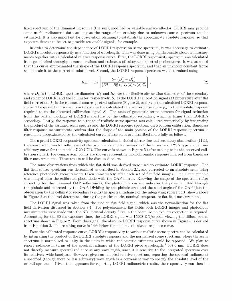
The a priori LORRI responsivity spectrum calculation included mirror size and secondary obscuration (11%),the measured curves for reflectance of the two mirrors and transmission of the lenses, and E2V’s typical quantumefficiency curve for the model 47-20 CCD. The curve is shown in Figure 5 (after scaling to fit the observed cali-bration signal). For comparison, points are shown representing monochromatic response inferred from bandpassfilter measurements. These results will be discussed below.

The same observations from which the flat field was derived were used to estimate LORRI response. Theflat field source spectrum was determined as described in Section 2.1, and corrected to an absolute scale usingreference photodiode measurements taken immediately after each set of flat field images. The 1 mm pinholewas imaged onto the calibrated photodiode with the OAP mirror. Knowing the shape of the spectrum (aftercorrecting for the measured OAP reflectance), the photodiode current indicates the power emitted throughthe pinhole and collected by the OAP. Dividing by the pinhole area and the solid angle of the OAP (less theobscuration by the collimator secondary) yields the spectral radiance of the integrating sphere port, shown abovein Figure 2 at the level determined during the panchromatic, nominal temperature flat field measurements.

The LORRI signal was taken from the median flat field signal, which was the normalization for the flatfield derivation discussed in Section 3.4. For polychromatic flat fields both LORRI images and photodiodemeasurements were made with the ND1 neutral density filter in the beam, so no explicit correction is required.Accounting for the 80 ms exposure time, the LORRI signal was 15908 DN/s/pixel viewing the diffuse sourcespectrum shown in Figure 2. From this signal, the absolute LORRI response curve shown in Figure 5 is derivedfrom Equation 2. The resulting curve is 14% below the nominal calculated response curve.

From the calibrated response curve, LORRI’s responsivity to various realistic scene spectra can be calculatedby integrating the product of the LORRI absolute response and the normalized scene spectrum, where the scenespectrum is normalized to unity in the units in which radiometric estimates would be reported. We plan toreport radiance in terms of the spectral radiance at the LORRI pivot wavelength,3 607.6 nm. LORRI doesnot directly measure spectral radiance at any wavelength, since it is sensitive to the integrated spectrum overits relatively wide bandpass. However, given an adopted relative spectrum, reporting the spectral radiance ata specified (though more or less arbitrary) wavelength is a convenient way to specify the absolute level of theoverall spectrum. Given this approach for reporting LORRI radiometric results, the responsivity can then be

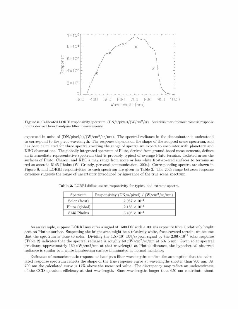
Figure 5. Calibrated LORRI responsivity spectrum, (DN/s/pixel)/(W/cm2/sr). Asterisks mark monochromatic responsepoints derived from bandpass filter measurements.

expressed in units of (DN/pixel/s)/(W/cm2/sr/nm). The spectral radiance in the denominator is understoodto correspond to the pivot wavelength. The response depends on the shape of the adopted scene spectrum, andhas been calculated for three spectra covering the range of spectra we expect to encounter with planetary andKBO observations. The globally integrated spectrum of Pluto, derived from ground-based measurements, definesan intermediate representative spectrum that is probably typical of average Pluto terrains. Isolated areas thesurfaces of Pluto, Charon, and KBO’s may range from more or less white frost-covered surfaces to terrains asred as asteroid 5145 Pholus (W. Grundy, personal communication, 2004). Corresponding spectra are shown inFigure 6, and LORRI responsivities to each spectrum are given in Table 2. The 20% range between responseextremes suggests the range of uncertainty introduced by ignorance of the true scene spectrum.

Table 2. LORRI diffuse source responsivity for typical and extreme spectra.

Spectrum Responsivity (DN/s/pixel) / (W/cm2/sr/nm)

Solar (frost) 2.957× 1011

Pluto (global) 2.186× 1011

5145 Pholus 3.406× 1011

As an example, suppose LORRI measures a signal of 1500 DN with a 100 ms exposure from a relatively brightarea on Pluto’s surface. Suspecting the bright area might be a relatively white, frost-covered terrain, we assumethat the spectrum is close to solar. Dividing the 1.5×104 DN/s/pixel signal by the 2.96×1011 solar response(Table 2) indicates that the spectral radiance is roughly 50 nW/cm2/sr/nm at 607.6 nm. Given solar spectralirradiance approximately 160 nW/cm2/nm at that wavelength at Pluto’s distance, the hypothetical observedradiance is similar to a white Lambertian surface illuminated at normal incidence.

Estimates of monochromatic response at bandpass filter wavelengths confirm the assumption that the calcu-lated response spectrum reflects the shape of the true response curve at wavelengths shorter than 700 nm. At700 nm the calculated curve is 17% above the measured value. The discrepancy may reflect an underestimateof the CCD quantum efficiency at that wavelength. Since wavelengths longer than 650 nm contribute about

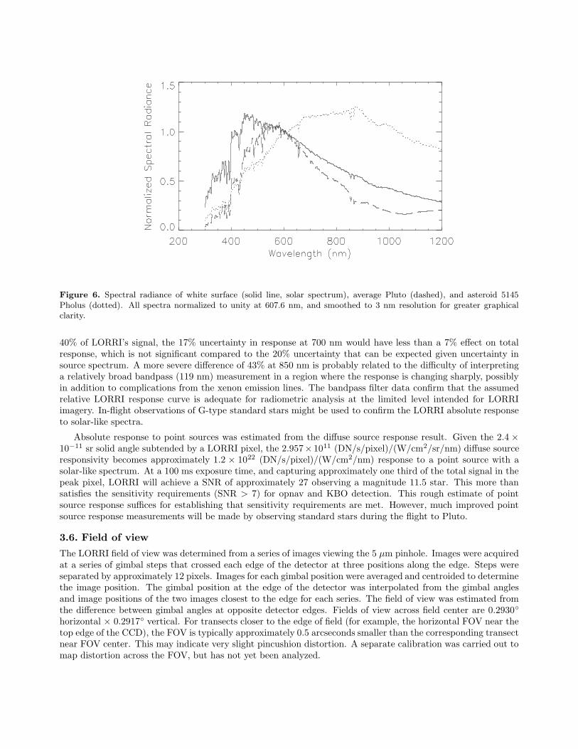
Figure 6. Spectral radiance of white surface (solid line, solar spectrum), average Pluto (dashed), and asteroid 5145Pholus (dotted). All spectra normalized to unity at 607.6 nm, and smoothed to 3 nm resolution for greater graphicalclarity.

40% of LORRI’s signal, the 17% uncertainty in response at 700 nm would have less than a 7% effect on totalresponse, which is not significant compared to the 20% uncertainty that can be expected given uncertainty insource spectrum. A more severe difference of 43% at 850 nm is probably related to the difficulty of interpretinga relatively broad bandpass (119 nm) measurement in a region where the response is changing sharply, possiblyin addition to complications from the xenon emission lines. The bandpass filter data confirm that the assumedrelative LORRI response curve is adequate for radiometric analysis at the limited level intended for LORRIimagery. In-flight observations of G-type standard stars might be used to confirm the LORRI absolute responseto solar-like spectra.

Absolute response to point sources was estimated from the diffuse source response result. Given the 2.4 ×

10−11 sr solid angle subtended by a LORRI pixel, the 2.957× 1011 (DN/s/pixel)/(W/cm2/sr/nm) diffuse sourceresponsivity becomes approximately 1.2 × 1022 (DN/s/pixel)/(W/cm2/nm) response to a point source with asolar-like spectrum. At a 100 ms exposure time, and capturing approximately one third of the total signal in thepeak pixel, LORRI will achieve a SNR of approximately 27 observing a magnitude 11.5 star. This more thansatisfies the sensitivity requirements (SNR > 7) for opnav and KBO detection. This rough estimate of pointsource response suffices for establishing that sensitivity requirements are met. However, much improved pointsource response measurements will be made by observing standard stars during the flight to Pluto.

3.6. Field of view

The LORRI field of view was determined from a series of images viewing the 5 µm pinhole. Images were acquiredat a series of gimbal steps that crossed each edge of the detector at three positions along the edge. Steps wereseparated by approximately 12 pixels. Images for each gimbal position were averaged and centroided to determinethe image position. The gimbal position at the edge of the detector was interpolated from the gimbal anglesand image positions of the two images closest to the edge for each series. The field of view was estimated fromthe difference between gimbal angles at opposite detector edges. Fields of view across field center are 0.2930◦

horizontal × 0.2917◦ vertical. For transects closer to the edge of field (for example, the horizontal FOV near thetop edge of the CCD), the FOV is typically approximately 0.5 arcseconds smaller than the corresponding transectnear FOV center. This may indicate very slight pincushion distortion. A separate calibration was carried out tomap distortion across the FOV, but has not yet been analyzed.

4. CONCLUSION

Calibration measurements have characterized LORRI’s detector parameters, and flat field and point source per-formance have been verified. Radiometric response to diffuse and point sources has been estimated; radiometricinterpretation of panchromatic imagery is always ambiguous when scene spectra are unknown, but the responsehas been calculated for a realistic range of scene spectra and useful radiometric information will be derivablefrom LORRI data despite the modest ambiguity. The flat field results may be corrected or replaced in flightdue to difficulties establishing accuracy at the desired 0.5% level over limited regions of the FOV, because of theghost and the particulate contamination. Also, although point source imaging performance has been verified toremain stable over temperature, accurate determination of the PSF awaits in-flight stellar observations. Overall,the instrument is well understood and ready to provide unprecedented imagery at Pluto and Charon and theKuiper belt.

ACKNOWLEDGMENTS

The LORRI calibration team would like to acknowledge Lana Pryde of Newport/SpectraPhysics/Oriel for helpfuladvice on selection of arc lamp light source components, and Brian Lai and Ken Ashton of Labsphere forengineering the integrating sphere. LORRI calibration was funded under NASA contract NAS 5-97271.

REFERENCES

1. S. Conard, F. Azad, J. Boldt, A. Cheng, K. Cooper, E. Darlington, , M. Grey, J. Hayes, P. Hogue,K. Kosakowski, T. Magee, M. Morgan, E. Rossano, D. Sampath, C. Schlemm, and H. Weaver, “Designand fabrication of the New Horizons Long-Range Reconnaissance Imager,” in Astrobiology and Planetary

Missions, G. R. Gladstone, ed., Proc. SPIE 5906, 2005.

2. M. Quijada, J. Stock, R. Boucarut, T. Saha, T. Madison, and T. Zukowski, “Optical stimulus for the cali-bration of the ultraviolet and optical telescope (uvot) for swift,” in X-Ray and Gamma-Ray Instrumentation

for Astronomy XIII, K. Flanagan and O. Siegmund, eds., Proc. SPIE 5165, 2004.

3. K. Horne, The ways of our errors: optimal data analysis for beginners and experts, star-www.st-and.ac.uk/ kdh1/pub0/ada/woe/woe.ps, University of St. Andrews, 2004.