Working Paper Series No: 2015/13

LARGE FIRM DYNAMICS AND THE BUSINESS CYCLE

Do large firm dynamics drive the business cycle? We answer this question by developing a quantitative theory of aggregate fluctuations caused by firm-level disturbances alone. We show that a standard heterogeneous firm dynamics setup already contains in it a theory of the business cycle, without appealing to aggregate shocks. We offer a complete analytical characterization of the law of motion of the aggregate state in this class of models – the firm size distribution – and show that the resulting closed form solutions for aggregate output and productivity dynamics display: (i) persistence, (ii) volatility and (iii) time-varying second moments. We explore the key role of moments of the firm size distribution – and, in particular, the role of large firm dynamics – in shaping aggregate fluctuations, theoretically, quantitatively and in the data.

Vasco M. Carvalho Basile Grassi (University of Cambridge) (University of Oxford)

Cambridge-INET Institute

Faculty of Economics

Large Firm Dynamics and the Business Cycle∗

Vasco M. Carvalho† Basile Grassi‡

April, 7, 2015

[ Link to the latest version]

Abstract

Do large firm dynamics drive the business cycle? We answer this question by developing

a quantitative theory of aggregate fluctuations caused by firm-level disturbances alone.

We show that a standard heterogeneous firm dynamics setup already contains in it a

theory of the business cycle, without appealing to aggregate shocks. We offer a complete

analytical characterization of the law of motion of the aggregate state in this class of

models – the firm size distribution – and show that the resulting closed form solutions for

aggregate output and productivity dynamics display: (i) persistence, (ii) volatility and

(iii) time-varying second moments. We explore the key role of moments of the firm size

distribution – and, in particular, the role of large firm dynamics – in shaping aggregate

fluctuations, theoretically, quantitatively and in the data.

Keywords: Large Firm Dynamics; Firm Size Distribution; Random Growth; Aggregate Fluctuations

∗The authors would like to acknowledge helpful comments from Arpad Abraham, Axelle Arquie, Florin Bilbiie, David

Backus, Paul Beaudry, Ariel Burstein, Jeff Campbell, Francesco Caselli, Gian Luca Clementi, Julian di Giovanni, Jan

Eeckhout, Xavier Gabaix, Wouter den Haan, Hugo Hopenhayn, Jean Imbs, Oleg Itskhoki, Boyan Jovanovic, Andrei

Levchenko, Isabelle Mejean, Ezra Oberfield, Michael Peters, Morten Ravn, Esteban Rossi-Hansberg, Edouard Schaal,

Rob Shimer and Gianluca Violante. The authors thank seminar participants at Banque de France, CREi, CREST-

INSEE, EUI, Essex, LSE, NYU, Princeton, NY Fed, Oxford, PSE, UCL and the Conference in Honor of Lars Hansen at

the University of Chicago. We thank Margit Reischer for excellent research assistance. Part of this work was carried out

during Grassi’s stay at the NYU Economics department and he is grateful for their hospitality. Carvalho acknowledges

the financial support of the European Research Council grant #337054, the Cambridge-INET Institute and the Keynes

Fellowship.†University of Cambridge and CREi, Universitat Pompeu Fabra, Barcelona GSE and CEPR. vcarvalho@crei.cat‡Nuffield College, Department of Economics, University of Oxford. basile.grassi@economics.ox.ac.uk

1

1 Introduction

Aggregate prices and quantities exhibit persistent dynamics and time-varying volatil-

ity. Business cycle theories have typically resorted to exogenous aggregate shocks in

order to generate such features of aggregate fluctuations. A recent literature has in-

stead proposed that the origins of business cycles may be traced back to micro-level

disturbances.1 Intuitively, the prominence of a small number of firms leaves open the

possibility that aggregate outcomes may be affected by the dynamics of large firms.2

And yet, we lack a framework that enables a systematic evaluation of the link between

the micro-level decisions driving firm growth, decline and churning and the persistence

and volatility of macro-level outcomes.

This paper seeks to evaluate the impact of large firm dynamics on aggregate fluctua-

tions. Building on a standard firm dynamics setup, we develop a quantitative theory of

aggregate fluctuations arising from firm-level shocks alone. We derive a complete ana-

lytical characterization of the law of motion of the firm size distribution – the aggregate

state variable in this class of models – and show that the resulting aggregate output

and productivity dynamics are endogenously (i) persistent, (ii) volatile and (iii) exhibit

time-varying second moments. We explore the key role of moments of the firm size dis-

tribution – and, in particular, the role of large firm dynamics – in shaping aggregate

fluctuations, theoretically, quantitatively and in the data. Our results imply that large

firm dynamics induce sizeable movements in aggregates and account for one quarter of

aggregate fluctuations.

Our setup follows Hopenhayn’s (1992) industry dynamics framework closely. Firms

differ in their idiosyncratic productivity level, which is assumed to follow a discrete

Markovian process. Incumbents have access to a decreasing returns to scale technology

using labor as the only input. They produce a unique good in a perfectly competitive

market. They face an operating fixed cost in each period which, in turn, generates

1See Gabaix (2011), Acemoglu et al. (2012), di Giovanni and Levchenko (2012), Carvalho andGabaix (2013) and di Giovanni, Levchenko and Mejean (2014)

2For example, in the fall of 2012, JP Morgan predicted that the upcoming “release of the iPhone5 could potentially add between 1/4 to 1/2%-point to fourth quarter annualized GDP growth” (JPMorgan, 2012). Apple’s prominence in the US economy is comparable to that of a small number ofvery large firms. For example, Walmart’s 2014 US sales amounted to 1.9% of US GDP. Taken together,according to Business Dynamics Statistics (BDS) data, the largest 0.02% of US firms account for about20% of all employment.

2

endogenous exit. As previous incumbents exit the market, they are replaced by new

entrants.

The crucial difference relative to Hopenhayn (1992) – and much of the large literature

that follows from it – is that we do not rely on the traditional “continuum of firms”

assumption in order to characterize the law of motion for the firm size distribution.

Instead, we characterize the law of motion for any finite number of firms. Our first

theoretical result shows that, generically, the firm size distribution is time-varying in a

stochastic fashion. As is well known, this distribution is the aggregate state variable

in this class of models. An immediate implication of our findings is therefore that

aggregate productivity, aggregate output and factor prices are themselves stochastic. In

a nutshell, we show that the standard workhorse model in the firm dynamics literature

– once the assumption regarding a continuum of firms is dropped – already features

aggregate fluctuations.

We then specialize our model to the case of random growth dynamics at the firm

level. Given our focus on large firm dynamics, the evidence put forth by Hall (1987)

in favor of Gibrat’s law for large firms makes this a natural baseline to consider.3

With this assumption in place, our second main theoretical contribution is to solve

analytically for the law of motion of the aggregate state in our model. This closed form

characterization is key to our analysis and enables us to provide a sharp characterization

of the equilibrium firm size distribution and the dynamics of aggregates.

Our third theoretical result is to show that the steady state firm size distribution is

Pareto distributed. We discuss the role of random growth, entry and exit and decreasing

returns to scale in generating this result. The upshot of this is that our model can

endogenously deliver a first-order distributional feature of the data: the co-existence

of a large number of small firms and a small, but non-negligible, number of very large

firms, orders of magnitude larger than the average firm in the economy.

Our final set of theoretical results sheds light on the micro origins of aggregate persis-

tence, volatility and time-varying uncertainty. Leveraging on our characterization of

the law of motion of the aggregate state we are able to show, analytically, that: (i) per-

sistence in aggregate output is increasing with firm level productivity persistence and

with the share of economic activity accounted by large firms; (ii) aggregate volatility

decays only slowly with the number of firms in the economy, and that this rate of decay

3See also Evans (1987) and the discussion in Luttmer (2010).

3

is generically a function of the size distributions of incumbents and entrants, as well

as the degree of decreasing returns to scale and (iii) aggregate volatility dynamics are

endogenously driven by the evolution of the cross-sectional dispersion of firm sizes.

We then explore the quantitative implications of our setup. Due to our characterization

of aggregate state dynamics, our numerical strategy is substantially less computational

intensive than that traditionally used when solving for heterogeneous agents’ models.

This allows us to solve the model featuring a very large number of firms and thus match

the firm size distribution accurately.

Our first set of quantitative results shows that the standard model of firm dynamics with

no aggregate shocks is able to generate sizeable fluctuations in aggregates: aggregate

output (aggregate productivity) fluctuations amount to 26% (17%, respectively) of that

observed in the data. These fluctuations have their origins in large firm dynamics. In

particular, we show how fluctuations at the upper end of the firm size distribution –

induced by shocks to very large firms – lead to movements in aggregates. We supplement

this analysis by showing that the same correlation holds true empirically: aggregate

output and productivity fluctuations in the data coincide with movements in the tail

of the firm size distribution.

We then focus on the origins of time-varying aggregate volatility. Consistently with our

analytical characterization, our quantitative results show that the evolution of aggregate

volatility is determined by the evolution of the cross-sectional dispersion in the firm size

distribution. Unlike the extant literature, the latter is the endogenous outcome of firm-

level idiosyncratic shocks and not the result of exogenous aggregate second moment

shocks. Again, we compare these results against the data and find consistent patterns:

aggregate volatility is high whenever cross-sectional dispersion high.

The paper relates to two distinct literatures: an emerging literature on the micro-origins

of aggregate fluctuations and the more established firm dynamics literature. Gabaix’s

(2011) seminal work introduces the “Granular Hypothesis”: whenever the firm size

distribution is fat tailed, idiosyncratic shocks average out at a slow enough rate that

it is possible for these to translate into aggregate fluctuations.4 Relative to Gabaix

(2011), our main contribution is to ground the granular hypothesis in a well specified

firm dynamics setup: in our setting, firms’ entry, exit and size decisions reflect optimal

4Other contributions in this literature include Acemoglu et al. (2012), di Giovanni and Levchenko(2012), Carvalho and Gabaix (2013) and di Giovanni, Levchenko and Mejean (2014).

4

forward-looking choices, given firm-specific productivity processes and (aggregate) fac-

tor prices. Further, the firm size distribution is an equilibrium object of our model.5

This allows us to both generalize the existent theoretical results and to quantify their

importance. The recent contribution of di Giovanni, Levchenko and Mejean (2014)

provides a valuable empirical benchmark to this literature and, in particular, to our

quantification exercise discussed above. Working with census data for France, their

variance decomposition exercise finds that large firm dynamics account for just under

20% of aggregate volatility. Our quantitative results show that the magnitude of ag-

gregate fluctuations implied by our firm dynamics environment is of the same order of

magnitude.

This paper is also related to the firm dynamics literature that follows from the seminal

contribution of Hopenhayn (1992).6 Some papers in this literature have explicitly stud-

ied aggregate fluctuations in a firm dynamics framework (Campbell and Fisher (2004),

Lee and Mukoyama (2008), Clementi and Palazzo (2015) and Bilbiie et al. (2012)). A

more recent strand of this literature has focused on the time-varying nature of aggre-

gate volatility and its link with the cross-sectional distribution of firms (e.g. Bloom

et al, 2014). Invariably, in this literature, business cycle analysis is restricted to the

case of common, aggregate shocks which are superimposed on firm-level disturbances.

Relative to this literature, we show that its standard workhorse model – once the as-

sumption regarding a continuum of firms is dropped and the firm size distribution is

fat tailed – already contains in it a theory of aggregate fluctuations and time-varying

aggregate volatility. We show this both theoretically and quantitatively in an otherwise

transparent and well understood setup. We eschew the myriad of frictions - capital

adjustment costs, labor market frictions, credit constraints or limited substitution pos-

sibilities across goods - that Hopenhayn’s (1992) framework has been able to support.

We do this because our focus is on large firm dynamics which are arguably less encum-

bered by such frictions.

The paper is organized as follows. Section 2 presents the basic model setup. Sections 3

and 4 develop our theoretical results. Section 5 describes the calibration of the model,

5The interplay between the micro-level decisions of firms and the equilibrium size distribution isalso the object of analysis in Luttmer (2007, 2010 and 2012). Relative to this body of work, ourcontribution is to focus on the implications of firm dynamics on aggregate fluctuations rather thanlong-run growth paths.

6See, for example, Campbell (1998), Veracierto (2002), Clementi and Hopenhayn (2006), Rossi-Hansberg and Wright (2007), Khan and Thomas (2008) and Acemoglu and Jensen (2015).

5

our quantitative results and our empirical exercises. Finally, Section 6 concludes.

2 Model

We analyze a standard firm dynamics setup (Hopenhayn, 1992) with a finite but possibly

large number of firms. We show how to solve for and characterize the evolution of the

firm size distribution without relying on the usual law of large numbers assumption. We

prove that, in this setting, the firm size distribution does not converge to a stationary

distribution, but instead fluctuates stochastically around it. As a result, we show that

aggregate prices and quantities are not constant over time as the continuum assumption

in Hopenhayn (1992) - repeatedly invoked by the subsequent literature - does not apply.

To do this, we start by describing the economic environment. As is standard in this class

of models, this involves specifying a firm-level productivity process, the incumbents’

problem and the entrants’ problem.

2.1 Model Setup

The setup follows Hopenhayn (1992) closely. Firms differ in their productivity level,

which is assumed to follow a discrete Markovian process. Incumbents have access to a

decreasing returns to scale technology using labor as the only input. They produce a

unique good in a perfectly competitive market. They face an operating cost at each pe-

riod, which in turn generates endogenous exit. There is also a large (but finite) number

of potential entrants that differ in their productivity. To operate next period, potential

entrants have to pay an entry cost. The economy is closed in a partial equilibrium

fashion by specifying a labor supply function that increases with the wage.

Productivity Process

We assume a finite but potentially large number of idiosyncratic productivity levels.

The productivity space is thus described by a S-tuple Φ := {ϕ1, . . . ,ϕS} with ϕ > 1

such that ϕ1 < . . . < ϕS. The idiosyncratic state-space is evenly distributed in logs,

where ϕ is the log step between two productivity levels: ϕs+1

ϕs = ϕ. A firm is in state

(or productivity state) s when its idiosyncratic productivity is equal to ϕs. Each firm’s

productivity level is assumed to follow a Markov chain with a transition matrix P .

6

We denote F (.|ϕs) as the conditional distribution of the next period’s idiosyncratic

productivity ϕs′ given the current period’s idiosyncratic productivity ϕs.7

Incumbents’ Problem

The only aggregate state variable of this model is the distribution of firms on the set

Φ. We denote this distribution by a (S × 1) vector µt giving the number of firms at

each productivity level s at time t. For the current setup description, we abstract from

explicit time t notation, but will return to it when we characterize the law of motion

of the aggregate state. Given an aggregate state µ, and an idiosyncratic productivity

level ϕs, the incumbent solves the following static profit maximization problem:

π∗(µ,ϕs) = Maxn

{ϕsnα − w(µ)n− cf}

where n is the labor input, w(µ) is the wage for a given aggregate state µ, and cf is

the operating cost to be paid every period. It is easy to show that π∗ is increasing in

ϕs and decreasing in w for a given aggregate state µ. The output of a firm is then

y(µ,ϕs) = (ϕs)1

1−α

(α

w(µ)

) α1−α

. In what follows, the size of a firm will refer to its output

level if not otherwise specified.

The timing of decisions for incumbents is standard and described as follows. The

incumbent first draws its idiosyncratic productivity ϕs at the beginning of the period,

pays the operating cost cf and then hires labor to produce. It then decides whether

to exit at the end of the period or to continue as an incumbent the next period. We

denote the present discounted value of being an incumbent for a given aggregate state

µ and idiosyncratic productivity level ϕs by V (µ,ϕs), defined by the following Bellman

Equation:

V (µ,ϕs) = π∗(µ,ϕs) + max

⎧⎨

⎩0, β

∫

µ′∈Λ

∑

ϕs′∈Φ

V (µ′,ϕs′)F (ϕs′|ϕs)Γ(dµ′|µ)

⎫⎬

⎭

where β is the discount factor, Γ(.|µ) is the conditional distribution of µ′, tomorrow’s

aggregate state and F (.|ϕs) is the conditional distribution of tomorrow’s idiosyncratic

productivity for a given today’s idiosyncratic productivity of the incumbent.

7That is, for a given productivity level ϕs, the distribution F (.|ϕs) is given by the sth-row vectorof the matrix P .

7

The second term on the right hand side of the value function above encodes an en-

dogenous exit decision. As is standard in this framework, this decision is defined by a

threshold level of idiosyncratic productivity given an aggregate state. Formally, since

the instantaneous profit is increasing in the idiosyncratic productivity level, there is a

unique index s∗(µ) for each aggregate state µ, such that: (i) for ϕs ≥ ϕs∗(µ) the incum-

bent firm continues to operate next period and, conversely (ii) for ϕs ≤ ϕs∗(µ)−1 firm

decides to exit next period.

After studying the incumbents’ problem, we now turn to the problem of potential

entrants.

Entrants’ Problem

There is an exogenously given, constant and finite number of prospective entrants M .

Each potential entrant has access to a signal about their potential productivity next

period, should they decide to enter today. To do so, they have to pay a sunk entry cost

which, in turn, leads to an endogenous entry decision which is again characterized by a

threshold level of initial signals.

Formally, the entrants’ signals are distributed according G = (Gq)q∈[1...S], a discrete

distribution over Φ. There is a total of M potential entrants every period, so that the

MGq gives the number of potential entrants for each signal level ϕq. If a potential

entrant decides to pay the entry cost ce, then she will produce next period with a

productivity level drawn from F (.|ϕq). Given this, we can define the value of a potential

entrant with signal ϕq for a given the aggregate state µ as V e(µ,ϕq):

V e(µ,ϕq) = β

∫

µ′∈Λ

∑

ϕq′∈Φ

V (µ′,ϕq′)F (ϕq′|ϕq)Γ(dµ′|µ)

Prospective entrants pay the entry cost and produce next period if the above value is

greater or equal to the entry cost ce. As in the incumbent’s exit decision, this now

induces a threshold level of signal, e∗(µ), for a given aggregate state µ such that (i) for

ϕq ≥ ϕe∗(µ) the potential entrant starts operating next period and, conversely (ii) for

ϕq ≤ ϕe∗(µ)−1 the potential entrant decides not to do so.

For simplicity, henceforth we assume that the entry cost is normalized to zero: ce = 0

which in turn implies that ϕe∗(µ) = ϕs∗(µ).

8

Labor Market and Aggregation

We assume that the supply of labor at a given wage w is given by Ls(w) = Mwγ

with γ > 0. We assume that, for a given wage level, the labor supply function is a

linear function of M , the number of potential entrants. This assumption is necessary

because in what follows we will be interested in characterizing the behavior of aggregate

quantities and prices as we let M increase. Note that if total labor supply were to be

kept fixed, increasing M would lead to an increase in aggregate demand for labor.

Therefore, the wage would increase mechanically. We therefore make this assumption

to abstract from this mechanical effect of increasing M on the equilibrium wage.8

To find equilibrium wages, we derive aggregate labor demand in this economy. To do

this, note that if Yt is aggregate output, i.e. the sum of all individual incumbents’

output, then Yt = At(Ldt )

α where Ldt is the aggregate labor demand, the sum of all

incumbents’ labor demand in period t. At, aggregate total factor productivity, is then

given by:

At =

(Nt∑

i=1

(ϕsi,t)1

1−α

)1−α

where ϕsi,t is the productivity level at date t of the ith firm among the Nt operating

firms at date t. This can be rewritten by aggregating over all firms that have the same

productivity level:

At =

(S∑

s=1

µs,t (ϕs)

11−α

)1−α

= (B′µt)1−α (1)

where B is the (S × 1) vector of parameters((ϕ1)

11−α , . . . , (ϕS)

11−α

). As discussed

above, the distribution of firms µt across the discrete state space Φ = {ϕ1, . . . ,ϕS} is a

(S×1) vector equal to (µ1,t, . . . , µS,t) such that µs,t is equal to the number of operating

firms in state s at date t. By the same argument, it is easy to show that aggregate

labor demand is given by Ld(wt) =(

αAt

wt

) 11−α

. Note that the model behaves as a one

factor model with aggregate TFP At.

8More generally, any increasing function of M will be possible. For simplicity, we assume a linearfunction. This assumption ensures that the equilibrium wage is independent of the number of potentialentrants. To see this, note that given the labor market equilibrium condition (Equation 2), and underthis assumption, the equilibrium wage is now a function of µt := µt

M , the normalized productivitydistribution across productivity levels. Given that M is a parameter of the model, we can thereforeuse µt or µt interchangeably as the aggregate state variable.

9

The market clearing condition then equates labor supply and labor demand, i.e. Ls(wt) =

Ld(wt). Given date t productivity distribution µt, we can then solve for the equilibrium

wage to get:

wt =

(α

11−α

B′µt

M

) 1−αγ(1−α)+1

(2)

This last Equation leads to the following expression for aggregate output:

Yt = AtLαt (3)

From these expressions, note that the wage and aggregate output is fully pinned down

by the distribution µt. Given a current-period distribution of firms across productivity

levels we can solve for all equilibrium quantities and prices. We are left to understand

how this distribution evolves over time, i.e. how to solve for for Γ(.|µt), which is

addressed in the following section.

3 Aggregate State Dynamics and Uncertainty: Gen-

eral Results

In this section, we first show how to characterize the law of motion for the productivity

distribution, the aggregate state in this economy. We will prove that, generically, the

distribution of firms across productivity levels is time-varying in a stochastic fashion.

An immediate implication of this result is that aggregate productivity At and aggre-

gate prices are themselves stochastic as they are simply a function of this distribution.

Additionally, we then show that the characterization of the stationary firm produc-

tivity distribution offered in Hopenhayn (1992) is nested in our model when we take

uncertainty to zero.

Law of Motion of the Productivity Distribution

In a setting with a continuum of firms, Hopenhayn (1992) shows that by appealing to

a law of large numbers, the law of motion for the productivity distribution is in fact

deterministic. In the current setting, with a finite number of incumbents, a similar

10

!"#

!!

!

!!

"!!

#

!"#!"$ !"#

!!"!

!

!!"!

"!!"!

#

!"# !"$

!"#

!!"!

!

!!"!

"!!"!

#

!"# !"$!"#

!!

!

!!

"!!

#

!"#!"$

%&'()'**+,&-,-).+/

0)')(1,'*+21.,&-,-).+/

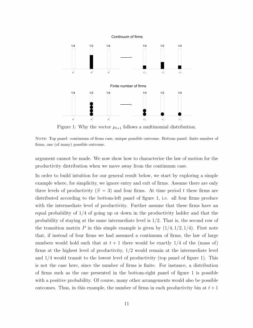
Figure 1: Why the vector µt+1 follows a multinomial distribution.

Note: Top panel: continuum of firms case, unique possible outcome. Bottom panel: finite number of

firms, one (of many) possible outcome.

argument cannot be made. We now show how to characterize the law of motion for the

productivity distribution when we move away from the continuum case.

In order to build intuition for our general result below, we start by exploring a simple

example where, for simplicity, we ignore entry and exit of firms. Assume there are only

three levels of productivity (S = 3) and four firms. At time period t these firms are

distributed according to the bottom-left panel of figure 1, i.e. all four firms produce

with the intermediate level of productivity. Further assume that these firms have an

equal probability of 1/4 of going up or down in the productivity ladder and that the

probability of staying at the same intermediate level is 1/2. That is, the second row of

the transition matrix P in this simple example is given by (1/4, 1/2, 1/4). First note

that, if instead of four firms we had assumed a continuum of firms, the law of large

numbers would hold such that at t + 1 there would be exactly 1/4 of the (mass of)

firms at the highest level of productivity, 1/2 would remain at the intermediate level

and 1/4 would transit to the lowest level of productivity (top panel of figure 1). This

is not the case here, since the number of firms is finite. For instance, a distribution

of firms such as the one presented in the bottom-right panel of figure 1 is possible

with a positive probability. Of course, many other arrangements would also be possible

outcomes. Thus, in this example, the number of firms in each productivity bin at t+ 1

11

follows a multinomial distribution with a number of trials of 4 and an event probability

vector (1/4, 1/2, 1/4)′.

In this simple example, all firms are assumed to have the same productivity level at

time t. It is easy however to extend this example to any initial arrangement of firms

over productivity bins. This is because, for any initial number of firms at a given

productivity level, the distribution of these firms across productivity levels next period

follows a multinomial. Therefore, the total number of firms in each productivity level

next period, is simply a sum of multinomials, i.e. the result of transitions from all

initial productivity bins.

More generally, for S productivity levels, and an (endogenous) finite number of incum-

bents, Nt, making optimal employment and production decisions and accounting for

entry and exit decisions, the following Theorem holds.

Theorem 1 The number of firms at each productivity level at t+1, given by the (S×1)

vector µt+1, conditional on the current vector µt, follows a sum of multinomial distri-

butions and can be expressed as:

µt+1 = m(µt) + ϵt+1 (4)

where ϵt+1 is a random vector with mean zero and a variance-covariance matrix Σ(µt)

and

m(µt) = (P ∗t )

′(µt +MG)

Σ(µt) =S∑

s=s∗(µt)

(MGs + µs,t)Ws

where P ∗t is the transition matrix P with the first (s∗(µt) − 1) rows replaced by zeros.

Ws = diag(Ps,.)− P′

s,.Ps,. where Ps,. denotes the s-row of the transition matrix P .

Proof. The distribution of firms µt across the discrete state space Φ = {ϕ1, . . . ,ϕS}

is a (S × 1) vector equal to (µ1,t, . . . , µS,t) such that µs,t is equal to the number of

operating firms in state s at date t. The next period’s distribution of firms across the

(discrete) state space Φ = {ϕ1, . . . ,ϕS} is given by the dynamics of both incumbents

and successful entrants.

12

In what follows, we define two conditional distributions. First, the distribution of

incumbent firms at date t+1 conditional on the fact that incumbents were in state s at

date t is denoted as f .,st+1. This (S×1) vector is such that for each state k in {1, . . . , S},

fk,st+1, the kth element of f .,s

t+1 gives the number of incumbents in state k at t + 1 which

were in state ϕs at t.

Similarly, let us define g.,st+1 the distribution of successful entrants at date t + 1 given

that they received the signal ϕs at date t. This (S × 1) vector is such that for each

state k in {1, . . . , S}, gk,st+1, the kth element of g.,st+1 gives the number of entrants in state

k at t + 1 which received a signal ϕs at t.

Period t + 1 distribution is the sum of all these conditional distributions and thus the

vector µt+1 satisfies:

µt+1 =S∑

s=s∗(µt)

f .,st+1 +

S∑

s=s∗(µt)

g.,st+1 (5)

Note that f .,st+1 and g.,st+1 are now multivariate random vectors implying that µt+1 also is

a random vector.

At date t+1 for s ≥ s∗(µt), f.,st+1 follows a multinomial distribution with two parameters:

the integer µs,t and the (S× 1) vector P ′s,. where Ps,. is the sth row vector of the matrix

P . Similarly, at date t + 1 for s ≥ s∗(µt), g.,st+1 follows a multinomial distribution with

two parameters: the integer MGq and the (S × 1) vector P ′q,..

Recall that the mean and variance-covariance matrix of a multinomial distribution,

M(m, h), is respectively the (S×1) vectormh and the (S×S) matrixH = diag(h)−hh′.

So let us define Ws = diag(Ps,.) − P′

s,.Ps,.. From the right hand side of Equation 5,

using the fact that the f .,st+1 and g.,st+1 follow multinomials, µt+1 has a mean m(µt) and a

variance-covariance matrix Σ(µt) where

m(µt) :=S∑

s=s∗(µt)

[µstP

′s,. +MGsP

′s,.

]= (P ∗

t )′(µt +MG)

Σ(µt) :=S∑

s=s∗(µt)

(MGs + µst)Ws

where P ∗t is the transition matrix P with the first (s∗(µt)− 1) rows replaced by zeros.

13

Equation 5 can be rewritten in a simple way as the sum of its mean and a zero-mean

shock:

µt+1 = m(µt) + ϵt+1

where

ϵt+1 =S∑

s=s∗(µt)

[f .,st+1 − µs

tP′

s,.

]+

S∑

s=s∗(µt)

[g.,st+1 −MGsP

′

s,.

]

i.e ϵt+1 is the demeaned version of µt+1. This gives us the result stated in the Theorem.

!

After taking into account the dynamics of incumbent firms and entry/exit decisions,

the law of motion (Equation 4) of the aggregate state – the distribution of firms over

productivity levels – is remarkably simple: tomorrow’s distribution is an affine func-

tion of today’s distribution up to a stochastic term, ϵt+1, that reshuffles firms across

productivity levels.

It is easy to understand this characterization by recalling our simple example economy

above without entry and exit. In this simple example, given the state transition proba-

bilities, we should for example observe that on average the number of firms remaining

at the intermediate level of productivity is twice that of those transiting to the highest

level of productivity. This is precisely what the affine part of Equation 4 captures: the

term m(µt) reflects these typical transitions, which are a function of matrix P alone.

However, with a finite number of firms, in any given period there will be stochastic

deviations from these typical transitions as we discuss above. In the Theorem, this is

reflected in the “reshuffling shock” term, ϵt+1, that enters in the law of motion given

by Equation 4. How important this reshuffling shock is for the evolution of the firm

distribution is dictated by the variance-covariance matrix Σ(µt) which, in turn, is a

function of the transition matrix P , the current firm distribution µt, and, in the general

case with entry and exit, the signal distribution available to potential entrants.

Dynamics Under No Aggregate Uncertainty

The above characterization - in particular, Equation 4 - is instructive of the differences

of the current setup relative to a standard Hopenhayn economy. The latter corresponds

to the case where all of the relevant firm dynamics are encapsulated by the affine

term m(µt). In order to understand this important benchmark case in the context

14

of our discussion, we now briefly define the stationary distribution that obtains when

the variance-covariance matrix is set to zero. Clearly, in this case, the aggregate state

µt becomes non-stochastic and our “reshuffling shock”, ϵt+1, operating on the cross-

sectional distribution of firms would be absent.

The following corollary to Theorem 1 shows that the dynamics of the productivity

distribution under no aggregate uncertainty are similar to the one in Hopenhayn (1992)

framework.9

Corollary 1 Let us define µt :=µt

M for any t. When aggregate uncertainty is absent,

ϵt+1 = 0:

µt+1 = (Pt)′(µt +G) (6)

where Pt is the transition matrix P where the first s(µt)− 1 rows are replaced by zeros,

and where s(µt) is the threshold of the exit/entry rule when the variance-covariance of

the ϵt+1 is zero.

Proof. This follows from Theorem 1 by taking Var[ϵt+1] = 0 and dividing both side

by M . !

Under this special case, the law of motion for the distribution of firms across produc-

tivity levels is deterministic and its evolution is given by Equation 6. An immediate

consequence of this is that under appropriate conditions on the transition matrix P , a

stationary distribution exists and is given by:

µ = (I − P ′)−1P ′G (7)

where P is the transition matrix P where the first (s(µ) − 1) rows are now replaced

by zeros to account for equilibrium entry and exit dynamics. In the current setting,

this is the analogue to Hopenhayn’s (1992) stationary distribution. Henceforth, we call

this object the stationary distribution, which can be interpreted as the deterministic

steady-state of our model.

Taking stock, we have derived a law of motion for any finite number of firms and shown

that, generically, the distribution of firms across productivity levels is time-varying in

a stochastic fashion. An immediate implication of this is that aggregate productivity

9Note that, as is clear from the example in Figure 1 and the proof of Theorem 1, assuming thatthere is no aggregate uncertainty is equivalent to assuming that there is a continuum of firms.

15

At is itself stochastic. Corollary 1 implies that, in the continuum case, the distribution

converges to a stationary object and, as a result, there are no aggregate fluctuations.

4 Aggregate State Dynamics under Gibrat’s Law

In this section, we analyze a special case of the Markovian process driving firm level

productivity: random growth dynamics. With this assumption in place, we then solve

for the law of motion of a sufficient statistic with respect to aggregate productivity.

By solving for this law of motion, we are then able to characterize how aggregate

fluctuations, aggregate persistence and time-varying aggregate volatility arise as an

endogenous feature of equilibrium firm dynamics.

4.1 Gibrat’s law implies power law in the steady state

We now specialize the general Markovian process driving the evolution of firm-level

productivity to the case of random growth. After exploring the firm-level implications

of this assumption, we revisit the steady-state results described in the previous section.

Assumption 1 Firm-level productivity evolves as a Markov Chain on the state spaceΦ = {ϕs}s=1..S with transition matrix

P =

⎛

⎜

⎜

⎜

⎜

⎜

⎝

a + b c 0 · · · · · · 0 0

a b c · · · · · · 0 0

· · · · · · · · · · · · · · · · · · · · ·

0 0 0 · · · a b c

0 0 0 · · · 0 a b + c

⎞

⎟

⎟

⎟

⎟

⎟

⎠

This is a restriction on the general Markov process P in section 2. It provides a parsimo-

nious parametrization for the evolution of firm-level productivity by only considering,

for each productivity level, the probability of improving, c, the probability of declin-

ing, a, and their complement, b = 1 − a − c, the probability of remaining at the same

productivity level. This process also embeds the assumption that there are reflecting

barriers in productivity, both at the top and at the bottom, inducing a well-defined

maximum and minimum level for firm-level productivity. This simple parametrization

will be key in obtaining the closed-form results below.

The Markovian process defined in Assumption 1 has been first introduced by Cham-

pernowne (1953) and Simon (1955) and studied extensively in Cordoba (2008). For

completeness, we now summarize the properties proved in the latter.

16

Properties 1 For a given firm i at time t with productivity level ϕsi,t following the

Markovian process in Assumption 1, we have the following:

1. The conditional expected growth rate and conditional variance of firm-level pro-

ductivity are given by

E

[ϕsi,t+1 − ϕsi,t

ϕsi,t|ϕsi,t

]= a(ϕ−1 − 1) + c(ϕ− 1)

Var

[ϕsi,t+1 − ϕsi,t

ϕsi,t|ϕsi,t

]= σ2

e

where σ2e is a constant. Both the conditional expected growth rate and the condi-

tional variance are independent of i’s productivity level, ϕsi,t.

2. As t → ∞, the probability of firm i having productivity level ϕs is

P (ϕsi,t = ϕs) −→t→∞

K (ϕs)−δ

where δ = log(a/c)logϕ and K is a normalization constant. Therefore, the stationary

distribution of the Markovian Process in Assumption 1 is Pareto with tail index

δ = log(a/c)logϕ .

In short, Cordoba (2008) shows that the Markov process in Assumption 1 is a con-

venient way to obtain Gibrat’s law on a discrete state space. In particular, Cordoba

(2008) shows that whenever firm-level productivity follows this process, its conditional

expected growth rate and its conditional variance are independent of the current level

(part 1 of the properties above). Importantly, Cordoba (2008) additionally shows that

the stationary distribution associated with this Markovian process is a power law dis-

tribution with tail index δ = log(a/c)logϕ (part 2 of the properties above).

The above assumption yields a tractable way of handling firm dynamics over time. At

several points of the analysis below we will also be interested in understanding how

the economy behaves with an ever larger number of firms. This raises the question of

whether the maximum possible level of firm-level productivity should be kept fixed. If

this was the case, and given the tight link between size and productivity implied by

our model, increasing the number of firms would imply a declining share of economic

activity commanded by the largest firms. As di Giovanni and Levchenko (2012) show

17

this is counter-factual: in cross-country data, whenever the number of firms is larger,

the share of the top firms in the economy increases. To accord with this evidence, in

the following assumption we allow the maximum productivity-level to increase with the

number of firms.

Assumption 2 Assume that ϕS = ZN1/δ

This assumption restricts the rate at which the maximum-level of productivity scales

with the number of firms. To understand why this is a natural restriction to impose,

first note that the stationary distribution of the Markovian process in Assumption 1

discussed above is also the cross-sectional distribution of a sample of size N of firms.

Since the former is power-law distributed so is the latter. Second, from Newman (2005),

the expectation of the maximum value of a sample N of random variables drawn from a

power law distribution with tail index δ is proportional to N1/δ. Thus, under Assump-

tion 2, for any sample of size N following the Markovian process in Assumption 1 the

stationary distribution of this sample is Pareto distributed with a constant tail index

δ.

With these two assumptions in place, we are now ready to revisit the main results in

the previous section. We start by characterizing further the stationary distribution in

Corollary 1, which we are now able to solve in closed-form. In particular, in Corollary

2 below we study the limiting case when the number of firms goes to infinity under

Assumptions 1 and 2.10

Corollary 2 Assume 1 and 2. If the potential entrants’ productivity distribution is

Pareto (i.e Gs = Ke (ϕs)−δe) then, as N → ∞, the stationary productivity distribution

converges point-wise to:

µs = K1

(ϕs

ϕs∗

)−δ

+K2

(ϕs

ϕs∗

)−δe

for s ≥ s∗

where δ = log(a/c)log(ϕ) and K1 and K2 are constants, independent of s and N .

10The proof of this Corollary is in two steps: (i) we first solve closed form for the stationary distri-bution given a maximum level of productivity ϕS under Assumption 1; (ii) we then take the limit ofthis distribution when the number of firms goes to infinity under the Assumption 2 stating how themaximum level of productivity scales with the number of firms.

18

Proof : See appendix A.1 !.

Thus, the stationary productivity distribution for surviving firms (i.e. for s ≥ s∗), is a

mixture of two Pareto distributions: (i) the stationary distribution of the Markovian

process assumed in 1 with tail index δ and (ii) the potential entrant distribution with

tail index δe.

The first of these distributions is a consequence of Gibrat’s law and a lower bound on the

size distribution. This works in a similar way to the existent random growth literature.

In the context of our model, this lower bound friction results from optimal entry and

exit decisions by firms. Every period there is a number of firms whose productivity

draws are low enough to induce to exit. These are replaced by low-productivity entrants

inducing bunching around the exit/entry threshold, s∗, as in Luttmer (2007, 2010, 2012)

. Unlike Luttmer however, our entrants can enter at every productivity level, according

to a Pareto distribution. This leads to the second term in the productivity distribution

above.

While the Corollary above characterizes the stationary firm-level productivity distribu-

tion it is immediate to apply these results to the firm size distribution. This is because

the firm size distribution maps one to one to µt. To see this, recall that the output of

a firm with productivity level ϕs is given by: ys = (ϕs)1

1−α

(αw

) α1−α . Therefore, in the

steady state, the number of firms of size ys is given by µs.

Our Corollary 2 therefore implies that, for sufficiently large firms, the tail of the firm size

distribution is Pareto distributed with tail index given by min{δ(1 − α), δe(1 − α)}.11

Note that the discrepancy between the firm (output) size distribution and the firm

productivity distribution is governed by the degree of returns to scale α. The higher

the degree of returns to scale, the lower the ratio between the productivity distribution

tail, δ, and the firm size distribution tail δ(1− α).

11To see this, note that for high productivity levels (i.e. for large s) the tail of the productivitydistribution is given by the smaller tail index, i.e. the fattest-tail distribution among the two.

19

4.2 Aggregate Dynamics: A Complete Characterization

With the above assumptions in place, we now offer a complete analytical character-

ization of the evolution of equilibrium aggregate output in our model. Recall from

Theorem 1 that we have already derived the law of motion of the aggregate state, i.e.

the productivity distribution, for any Markov process governing the evolution of firm-

level productivity. Under assumptions 1 and 2 we can specialize this law of motion to

the particular case of random growth dynamics at the firm-level.

In particular, we derive the law of motion of

Tt := B′µt =S∑

s=1

(ϕs)1

1−α µt,s

From the expressions for aggregate productivity (Equation 1) and the equilibrium wage

(Equation 2), it is immediate that Tt is a sufficient statistic to solve for the relative

price of labor in our model. By deriving the law of motion for Tt we are therefore able

to characterize the law of motion for aggregate prices, productivity and output.

Theorem 2 Assume 1 and 2. If the potential entrants’ productivity distribution is

Pareto (i.e Gs = Ke (ϕs)−δe) then,

Tt+1 = ρTt + ρEt(ϕ) +OTt + σtεt+1 (8)

σ2t = ϱDt + ϱEt(ϕ

2) +Oσt (9)

where E[εt+1] = 0 and Var[εt+1] = 1. The persistence of the aggregate state is ρ =

aϕ−11−α + b + cϕ

11−α . The net entry term is the difference between the entry and exit

contributions: Et(x) =(M∑S

s=stGs (xs)

11−α

)−((xst−1)

11−α µst−1,t

). The term Dt is

given by Dt :=∑S

s=st−1

((ϕs)

11−α

)2µs,t and ϱ = aϕ

−21−α + b+ cϕ

21−α − ρ2. The terms OT

t

and Oσt are a correction for the upper reflecting barrier in the idiosyncratic state space.

Proof: See appendix A.3 !.

Theorem 2 provides a full description of aggregate state dynamics in our model. It

can be understood intuitively in terms of the evolution of aggregate productivity by

noting that T (1−α)t = At, i.e. Tt is simply a convex function of aggregate productivity.

20

Thus, up to this transformation, the Theorem states that the aggregate productivity

of incumbents tomorrow is the sum of (i) ρTt, the expected aggregate productivity of

today’s incumbents, conditional on their survival, (ii) ρEt(ϕ), the expected aggregate

productivity of today’s net entrants conditional on their survival, and (iii) σtεt+1 a

mean zero aggregate productivity shock. The term OTt is a correction term, arising

from having imposed bounds on the state-space. This term vanishes as the state-space

bounds increase; we relegate its precise functional form and further discussion of this

term to the appendix.

Given the law of motion for the aggregate state, it is straightforward to characterize the

law of motion for equilibrium output in our model. Corollary 3 does this by describing

the dynamics of Yt+1, the percentage deviation of output from its steady-state value.

Corollary 3 Assume 1 and 2. If the potential entrants’ productivity distribution is

Pareto (i.e Gs = Ke (ϕs)−δe) then, aggregate output (in percentage deviation from steady

state) has the following law of motion:

Yt+1 = ρYt + ρκ1Et(ϕ) + κ2OTt +

σt

Tϵt+1 (10)

where σt is given by Equation 9, Et(ϕ) is the percentage deviation from steady-state

of Et(ϕ), OTt is the percentage deviation from steady-state of OT

t , κ1, κ2 are constants

defined in the appendix and T is the steady-state value of the aggregate state variable

Tt.

Proof: See appendix A.4 !.

The law of motion for Tt thus implies that aggregate output is persistent, as parametrized

by ρ, and displays time-varying volatility, given by σt. Again, it is worth noting that

there are no aggregate shocks or aggregate sources of persistence in our setting. Rather,

these two properties emerge from the aggregation of firm-level dynamics alone. To bet-

ter understand these aggregation results, and building on the expressions in Theorem

2 and Corollary 3, we now detail how persistence in aggregates depend on micro-level

parameters. We then turn our attention to the (firm-level) origins of time-varying

volatility in aggregates.

21

Aggregate Persistence

The following Proposition characterizes how the persistence of aggregate output, ρ,

depends on parameters governing firm-level dynamics.

Proposition 1 Let δ =log a

c

logϕ be the tail index of the stationary productivity distribution

as in Corollary 2. If δ ≥ 11−α then the persistence of the aggregate state, ρ, satisfies the

following properties:

i) Holding δ constant, aggregate persistence is increasing in firm-level persistence:∂ρ∂b ≥ 0

ii) Holding b constant, aggregate persistence is decreasing in the tail index of the

stationary productivity distribution: ∂ρ∂δ ≤ 0

iii) If the productivity distribution is Zipf, aggregate state dynamics contain a unit

root: if δ = 11−α , ρ = 1

Proof: See appendix A.5 !.

To interpret the condition under which the Proposition is valid, recall that δ(1−α) gives

the tail index of the stationary firm size distribution. Hence, the Proposition applies to

Pareto distributions that are (weakly) thinner than Zipf. According to the Proposition,

(i) the persistence of the aggregate state (and hence aggregate productivity, wages and

output) is increasing in the probability, b, that firms do not change their productivity

from one time period to the other. Intuitively, the higher is firm-level productivity

persistence, the more persistent are aggregates.12

Further, according to (ii) in the Proposition, aggregate persistence will decrease with

the tail index of the stationary firm-level productivity distribution. To understand this,

note that this tail index is given by ac . The thinner the tail, the larger this ratio is

and thus, the larger is the relative probability of a firm having a lower productivity

tomorrow. This therefore induces stronger mean reversion in productivity (and size) at

the firm level which, in turn, leads to lower aggregate persistence. Thus, a fatter tail

in the size distribution implies heightened aggregate persistence. In the limiting case

12Note that we are holding the tail index of the stationary productivity distribution, δ, constant. Interms of model primitives, we are keeping fixed the ratio a

c while maintaining the adding-up constrainta+ b+ c = 1.

22

where the stationary size distribution is given by Zipf’s law (δ(1−α) = 1 in case (iii)),

aggregate persistence is equal to 1. That is, Zipf’s law implies unit-root type dynamics

in aggregates.

(Time-Varying) Aggregate Volatility

We are now interested in understanding how aggregate volatility - and its evolution -

depend on the parameters driving the micro-dynamics. To do this, we find it convenient

to first rewrite the expression for the conditional volatility of Yt+1 as:

Vart[Yt+1

]=

σ2t

T 2= ϱ

D

T 2

Dt

D+ ϱ

E(ϕ2)

T 2

Et(ϕ2)

E(ϕ2)+

Oσ

T 2

Oσt

Oσ(11)

where T , E and D are the the steady-state counterparts of Tt, Et and Dt. To inter-

pret these objects, first recall that Dt =∑S

s=st−1

((ϕs)

11−α

)2µs,t is proportional to the

second moment of the firm size distribution at time t, a well defined measure of dis-

persion.13 D is therefore proportional to the steady state dispersion in firm size. By

the same argument, Et(ϕ2) =

(M∑S

s=st

((ϕs)

11−α

)2Gs

)−

(((ϕst−1)

11−α

)2µst−1,t

),

is proportional to dispersion of firm size among successful entrants 14 and E is the

corresponding object at the steady state.

Note also that the expression above implies that the unconditional expectation of con-

ditional variance can be written as:

Eσ2t

T 2= ϱ

D

T 2+ ϱ

E(ϕ2)

T 2+

Oσ

T 2(12)

With these two objects in place, the following Proposition characterizes how aggregate

volatility and its dynamics depend on the primitives of the model.

13To see this, recall that the size at time t of a firm with productivity level ϕs is given by

ys,t = (ϕs)1

1−α (α/wt)α

1−α . The second moment of the firm size distribution is then∑S

s=1 y2s,tµs,t =

∑Ss=1 (ϕ

s)2

1−α (α/wt)2α

1−α µs,t = (α/wt)2α

1−α Dt. In other words, Dt is proportional to the second mo-ment of the firm size distribution at time t.

14Where the last term in the expression corrects for exit, and is proportional to the dispersion inthe size of exiters.

23

Proposition 2 Let δ =log a

c

logϕ be the tail index of the stationary productivity distribution

as in Corollary 2. Let δe be the tail index associated with the productivity distribution

of potential entrants. Then

i) Under assumption 2 and if 1 < δ(1 − α) < 2 and 1 < δe(1 − α) < 2, the

unconditional expectation of aggregate variance satisfies:

E

[σ2t

T 2

]∼

N→∞

ϱD1

N2− 2δ(1−α)

+ϱD2

N1+ δeδ− 2

δ(1−α)

(13)

where D1 and D2 are functions of model parameters but independent of N and

M .

ii) The dynamics of conditional aggregate volatility depend on the dispersion of firm

size:∂Vart

[Yt+1

]

∂Dt=

∂Vart[Yt+1

]

∂Et=

ϱ

T 2≥ 0

Proof: See appendix A.6 !.

Part (i) of Proposition 2 characterizes the average level of volatility of aggregate output

growth in our model. It builds on our result that, under random growth dynamics for

firm-level productivity, the stationary incumbent size distribution is Pareto distributed.

It assumes further that the size distribution of potential entrants is also power law

distributed. The assumptions on δ(1−α) and δe(1−α) ensure that these distributions

are sufficiently fat tailed.

The ∼N→∞

notation means that, in expectation, the conditional variance of the aggregate

growth rate scales with N , the number of incumbent firms at the steady state, at a rate

that is equal to the rate of the expression on the right hand side. The latter reflects

the separate contributions of (i) surviving time t incumbents (i.e. the first term in the

expression) and that of (ii) time t entrants that start producing at t+1 (i.e. the second

term in the expression).

The key conclusion of the first part of Proposition 2 is therefore that, for 1 < δ(1−α) < 2

and 1 < δe(1 − α) < 2, the variance of aggregate growth scales at a slower rate than

1/N . Recall that the latter would be the rate of decay implied by a shock-diversification

argument relying on standard central limit Theorems. This is not the case when the

firm size distribution is fat tailed, as it is here. Rather, as the Proposition makes

24

clear, the rate of decay of aggregate volatility depends on the tail indexes of the size

distributions of entrants and incumbents. Whenever the size distribution of incumbents

has a lower tail index than the size distribution of entrants - i.e. whenever δ < δe - the

rate of decay of aggregate volatility is a function of the tail index of incumbents alone.

Conversely, whenever the size distribution of entrants has a fatter tail, the rate of decay

is a function of the tail behavior of both incumbents and entrants. For either case, the

closer are these distributions to Zipf’s law, the slower is the rate of the decay.

This Proposition thus generalizes the main result in Gabaix (2011) to an environment

where: (i) firm dynamics are the result of optimal intratemporal (i.e size) and in-

tertemporal firm-level decisions (i.e. exit and entry), given the idiosyncratic produc-

tivity process characterized by the Markovian process in Assumption 1 and (ii) the

Pareto distribution of firm sizes is an equilibrium outcome consistent with optimal firm

decisions. More generally, the first part of Proposition implies that the voluminous

literature that builds on the framework of Hopenhayn (1992) has overlooked the poten-

tially non-negligible aggregate dynamics implied by the model, even when the number

of firms entertained is large.

Part (ii) of Proposition 2 shows that the evolution of aggregate volatility over time –

i.e. the conditional variance of aggregate output – mirrors that of Dt. As discussed

above, Dt is proportional to the second moment of the firm size distribution at time t.

Thus, whenever the firm size distribution at time t is more dispersed than the stationary

distribution (Dt > D), aggregate volatility is higher.

The second part of the Proposition is therefore related to a literature looking at the

connection between micro and macro uncertainty (see Bloom et al, 2014 and Kehrig,

2014). Consistent with the results of this literature, the Proposition yields a direct,

positive, link between the two levels of uncertainty. Unlike this literature however, this

link between the cross-sectional dispersion of micro-units and conditional aggregate

volatility is endogenous and emerges without resorting to any exogenous aggregate

shocks influencing the first and second moments of firms’ growth.

5 Quantitative Results

In this section we present the quantitative implications of our model. We solve the

model under the particular case of firm-level random productivity growth, which we

25

have discussed in the previous section. We first calibrate the stationary steady-state

solution of the model to match firm-level moments.

Based on this calibration, we then use the law of motion of the aggregate state to solve

numerically for the firms’ policy function. Thanks to our analytical characterization,

our numerical strategy is substantially less computational intensive than that tradition-

ally used when solving for heterogeneous agents models under aggregate uncertainty.

This allows us to solve the model under a large-dimensional state-space. We discuss this

in detail below. Using this numerical solution we quantitatively assess the performance

of the model with respect to standard business cycle statistics and inspect the mech-

anism rendering firm-level idiosyncratic shocks into aggregate fluctuations. We then

quantitatively explore the role of large firms in shaping the business cycle. Throughout

we show empirical evidence that is consistent with our mechanism.

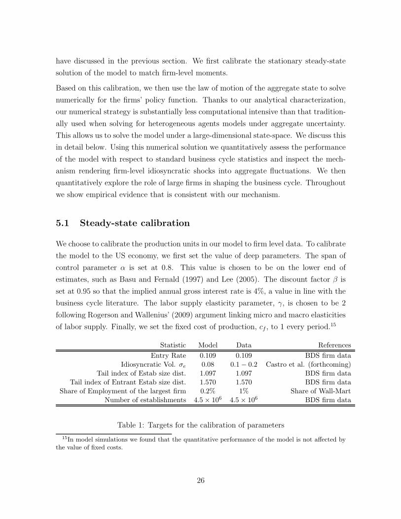
5.1 Steady-state calibration

We choose to calibrate the production units in our model to firm level data. To calibrate

the model to the US economy, we first set the value of deep parameters. The span of

control parameter α is set at 0.8. This value is chosen to be on the lower end of

estimates, such as Basu and Fernald (1997) and Lee (2005). The discount factor β is

set at 0.95 so that the implied annual gross interest rate is 4%, a value in line with the

business cycle literature. The labor supply elasticity parameter, γ, is chosen to be 2

following Rogerson and Wallenius’ (2009) argument linking micro and macro elasticities

of labor supply. Finally, we set the fixed cost of production, cf , to 1 every period.15

Statistic Model Data References

Entry Rate 0.109 0.109 BDS firm dataIdiosyncratic Vol. σe 0.08 0.1− 0.2 Castro et al. (forthcoming)

Tail index of Estab size dist. 1.097 1.097 BDS firm dataTail index of Entrant Estab size dist. 1.570 1.570 BDS firm data

Share of Employment of the largest firm 0.2% 1% Share of Wall-MartNumber of establishments 4.5× 106 4.5× 106 BDS firm data

Table 1: Targets for the calibration of parameters

15In model simulations we found that the quantitative performance of the model is not affected bythe value of fixed costs.

26

We then assume random productivity growth at the firm level, i.e. we follow Assumption

1 in the previous section. This implies that the stationary productivity distribution is

Pareto-distributed with tail index δ. We additionally assume that the productivity of

potential entrants is Pareto distributed with tail index δe. With these assumptions in

place, the behavior of the model is exactly characterized by Theorem 2. This will also

imply a Pareto distribution for firm size in the stationary steady state.

To obtain data counterparts for these and further moments discussed below, we use

publicly available tabulations of firm size and firm size by age from the Business Dy-

namics Statistics (BDS) data between 1977 and 2012. These are in turn computed from

the Longitudinal Business Database of the US census and ensure a near full coverage of

the population of US firms. For a full description of this dataset and our computations

below, please refer to the Data Appendix B.

According to our model, we can read off the tail of the productivity distribution of in-

cumbents from its empirical counterpart by using the relation δ(1−α) = 1.097 and our

assumed value for α. According to Corollary 2, this fixes the ratio between the param-

eters a and c in the firm-level productivity process, up to the state space parameter ϕ.

Similarly, we fix the tail index for entrant distribution such that δ(1 − α) = 1.570. To

obtain these numbers, we estimate the tail index from the BDS data at the US census.

The data counterpart to the stationary size distribution in our model is given by the

average (across years) of the size distribution of all firms. The corresponding object

for entrants is given by the average (across years) size distribution of age 0 firms in

the BDS data. We obtain tail estimates by using the estimator proposed in Virkar and

Clauset (2014). According to our estimates the size distribution of incumbents is more

fat tailed than that of the corresponding distribution of entrants; this is intuitive as

the probability of observing very large entrants should indeed be smaller. While we are

not aware of any such estimation for entrants, our tail index estimates for incumbents

compare well with published estimates by Axtell (2001), Gabaix (2011) and Luttmer

(2007).

We are left with two parameters to calibrate: the state space parameter ϕ and the

parameter governing persistence in firm-level productivity, b. We calibrate these pa-

rameters jointly to match the volatility of firm-level growth rates, σe = 8% and the

stationary entry rate, i.e. the ratio of entrants to incumbents, to be equal to 10.9%.

Our choice for firm-level volatility is an intentionally conservative choice relative to

27

the typical values reported in the literature. Working with Compustat data, Comin

and Phillipon (2006) and Davis et al (2007) report sales growth volatility estimates for

publicly listed firms between 0.1 and 0.2. Davis et al (2007) report even higher values

for employment volatility at privately held firms, based on the Longitudinal Database

of Businesses. Working with establishment level data, Foster et al (2008) and Castro

et al (forthcoming) report an average value for annual productivity (TFPR) volatility

of about 20% . By choosing a value for volatility at the lower end of these estimates,

we acknowledge that large firms are typically less volatile than the average firm. Our

choice for the entry rate target comes from computing the average entry rate from the

BDS data. This is consistent with, for example, the values reported by Dunne et al

(1988).16

Finally, we need to choose values for S and M . By choosing S we are fixing the largest

possible productivity of a firm. Our choice of S implies that the largest firm accounts

for 0.2% of total employment. This is again a conservative choice: Walmart for example

is reported to have 1.4 million employees based in the US, about 1% of the labor force

in the US. Recall that M is a free scale parameter as discussed in the setup of the

model. We calibrate M such that the total number of firms is about 4.5 million, the

mean total number of establishments reported in the BDS data. In table 1, we report

the establishment moments that we match for the calibration. In table 2, the implied

parameters by our targets.

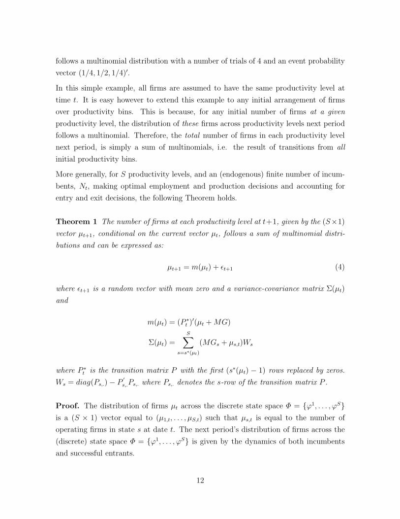
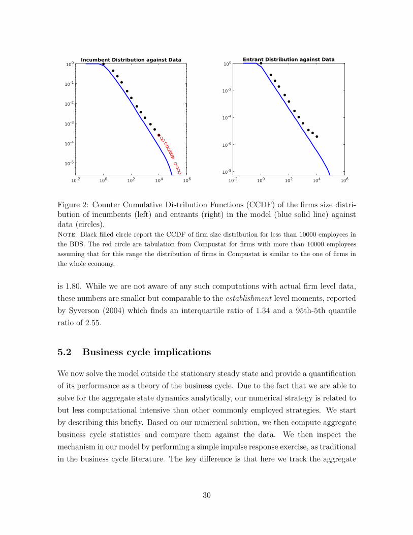
We are interested in accurately matching the characteristics of large firms. Recall that

our calibration procedure is intended to match well the tail of the firm size distribu-

tion. The left panel of Figure 2, plots the entire firm size distribution (in terms of

employees) as implied by our model against that in the data. The right panel plots

the corresponding distribution for entrants. These are plots of the counter-cumulative

(CCDF) distribution of firm size giving, in the x-axis, the employment size category of a

given firm and, in the y-axis, the empirical probability of finding a firm larger than the

corresponding x-axis employment size category. The solid line reports the stationary

size distribution in the model.

Filled (black) circles give the size distribution derived from the Business Dynamics

Statistics (BDS) from the US Census which we have used to estimate the tail index.

Note that the largest bin in the BDS data only pins down the minimum size of the

16We discuss in detail our data sources and computations in the Data Appendix.

28

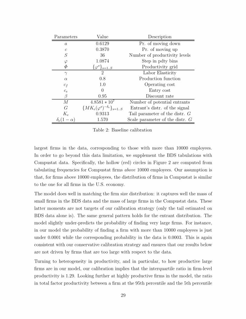
Parameters Value Description

a 0.6129 Pr. of moving downc 0.3870 Pr. of moving upS 36 Number of productivity levelsϕ 1.0874 Step in pdty binsΦ {ϕs}s=1..S Productivity gridγ 2 Labor Elasticityα 0.8 Production functioncf 1.0 Operating costce 0 Entry costβ 0.95 Discount rateM 4.8581 ∗ 107 Number of potential entrantsG {MKe(ϕs)−δe}s=1..S Entrant’s distr. of the signalKe 0.9313 Tail parameter of the distr. G

δe(1− α) 1.570 Scale parameter of the distr. G

Table 2: Baseline calibration

largest firms in the data, corresponding to those with more than 10000 employees.

In order to go beyond this data limitation, we supplement the BDS tabulations with

Compustat data. Specifically, the hollow (red) circles in Figure 2 are computed from

tabulating frequencies for Compustat firms above 10000 employees. Our assumption is

that, for firms above 10000 employees, the distribution of firms in Compustat is similar

to the one for all firms in the U.S. economy.

The model does well in matching the firm size distribution: it captures well the mass of

small firms in the BDS data and the mass of large firms in the Compustat data. These

latter moments are not targets of our calibration strategy (only the tail estimated on

BDS data alone is). The same general pattern holds for the entrant distribution. The

model slightly under-predicts the probability of finding very large firms. For instance,

in our model the probability of finding a firm with more than 10000 employees is just

under 0.0001 while the corresponding probability in the data is 0.0003. This is again

consistent with our conservative calibration strategy and ensures that our results below

are not driven by firms that are too large with respect to the data.

Turning to heterogeneity in productivity, and in particular, to how productive large

firms are in our model, our calibration implies that the interquartile ratio in firm-level

productivity is 1.29. Looking further at highly productive firms in the model, the ratio

in total factor productivity between a firm at the 95th percentile and the 5th percentile

29

10-2 100 102 104 106

10-5

10-4

10-3

10-2

10-1

100Incumbent Distribution against Data

—— 10-2 100 102 104 10610-8

10-6

10-4

10-2

100Entrant Distribution against Data

Figure 2: Counter Cumulative Distribution Functions (CCDF) of the firms size distri-bution of incumbents (left) and entrants (right) in the model (blue solid line) againstdata (circles).Note: Black filled circle report the CCDF of firm size distribution for less than 10000 employees in

the BDS. The red circle are tabulation from Compustat for firms with more than 10000 employees

assuming that for this range the distribution of firms in Compustat is similar to the one of firms in

the whole economy.

is 1.80. While we are not aware of any such computations with actual firm level data,

these numbers are smaller but comparable to the establishment level moments, reported

by Syverson (2004) which finds an interquartile ratio of 1.34 and a 95th-5th quantile

ratio of 2.55.

5.2 Business cycle implications

We now solve the model outside the stationary steady state and provide a quantification

of its performance as a theory of the business cycle. Due to the fact that we are able to

solve for the aggregate state dynamics analytically, our numerical strategy is related to

but less computational intensive than other commonly employed strategies. We start

by describing this briefly. Based on our numerical solution, we then compute aggregate

business cycle statistics and compare them against the data. We then inspect the

mechanism in our model by performing a simple impulse response exercise, as traditional

in the business cycle literature. The key difference is that here we track the aggregate

30

response to an idiosyncratic shock which endogenously translates into an aggregate

perturbation.

5.2.1 Numerical Strategy

The analytical solution to the law of motion of the aggregate state in Theorem 2 is key

to our numerical strategy. Recall that in the model firms make optimal intertemporal

decisions (entry and exit) by forming expectations of future aggregate conditions which

are summarized by the state variable Tt. As Theorem 2 renders clear, the dynamics of

Tt in turn depend on Dt, a term that is proportional to the second moment of the firm

size distribution. Since the firm size distribution is a stochastic and time-varying object

so is Dt. In order to solve the model numerically we will make the assumption that Dt

is perceived by firms to be fixed at its steady-state value. Given this assumption, the

firms’ problem can be solved by standard value function iteration methods. We discuss

this numerical algorithm in detail in Appendix C.

This is similar in spirit to the Krusell-Smith approach in that agents only take into

account a reduced set of moments of the underlying high-dimensional state variable.

Unlike Krusell and Smith (1998) however, we have a closed-form solution for the law

of motion of the first moment of this distribution and hence, in our numerical solution,

agents know the law of motion of Tt, up to second moments. In Krusell and Smith

(1998) this law of motion has to be solved for, which imposes a simulation step with

a high computational cost. Our procedure is also similar to that of Den Haan and

Rendahl (2010) in that we exploit recurrence Equations linking different moments of

the state distribution and then assume that agents’ expectations do not depend on

higher order moments of the distribution. Unlike them we do not need to solve for

the law of motion of these moments. The consequence of a lower computational cost

relative to the literature is that it allows us to solve for a large state space and therefore

to better capture firm-level heterogeneity in productivity.17

5.2.2 Business cycle statistics

Using the calibration in 2 and the numerical algorithm describes in Appendix C, we

compute the business cycle statistics. We simulate time series for output, hours and

17This solution method is arguably applicable to a large class of heterogeneous agents models when-ever these incorporate random growth processes.

31

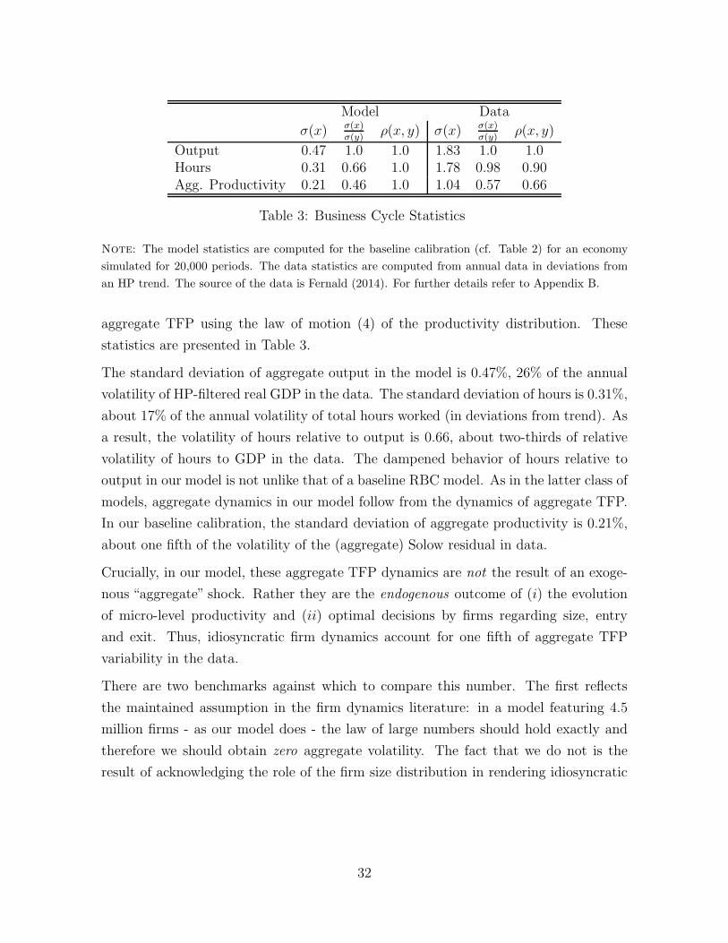
Model Data

σ(x) σ(x)σ(y) ρ(x, y) σ(x) σ(x)

σ(y) ρ(x, y)

Output 0.47 1.0 1.0 1.83 1.0 1.0Hours 0.31 0.66 1.0 1.78 0.98 0.90Agg. Productivity 0.21 0.46 1.0 1.04 0.57 0.66

Table 3: Business Cycle Statistics

Note: The model statistics are computed for the baseline calibration (cf. Table 2) for an economy

simulated for 20,000 periods. The data statistics are computed from annual data in deviations from

an HP trend. The source of the data is Fernald (2014). For further details refer to Appendix B.

aggregate TFP using the law of motion (4) of the productivity distribution. These

statistics are presented in Table 3.

The standard deviation of aggregate output in the model is 0.47%, 26% of the annual

volatility of HP-filtered real GDP in the data. The standard deviation of hours is 0.31%,

about 17% of the annual volatility of total hours worked (in deviations from trend). As

a result, the volatility of hours relative to output is 0.66, about two-thirds of relative

volatility of hours to GDP in the data. The dampened behavior of hours relative to

output in our model is not unlike that of a baseline RBC model. As in the latter class of

models, aggregate dynamics in our model follow from the dynamics of aggregate TFP.

In our baseline calibration, the standard deviation of aggregate productivity is 0.21%,

about one fifth of the volatility of the (aggregate) Solow residual in data.

Crucially, in our model, these aggregate TFP dynamics are not the result of an exoge-

nous “aggregate” shock. Rather they are the endogenous outcome of (i) the evolution

of micro-level productivity and (ii) optimal decisions by firms regarding size, entry

and exit. Thus, idiosyncratic firm dynamics account for one fifth of aggregate TFP

variability in the data.

There are two benchmarks against which to compare this number. The first reflects

the maintained assumption in the firm dynamics literature: in a model featuring 4.5

million firms - as our model does - the law of large numbers should hold exactly and

therefore we should obtain zero aggregate volatility. The fact that we do not is the

result of acknowledging the role of the firm size distribution in rendering idiosyncratic

32

disturbances into aggregate ones; as first emphasized by Gabaix (2011) and generalized

by our Proposition 2.18

The second benchmark is given by the recent empirical work of di Giovanni, Levchenko,

Mejean (2014). Using a database covering the universe of French firms they conclude

that firm-level idiosyncratic shocks account for about half of aggregate fluctuations

and that a quarter of this can in turn be attributed to the direct impact of large

firm dynamics on aggregates (the other three quarters being attributed to linkages

as in Acemoglu et al 2012). Our quantification gives a structural interpretation to

these numbers and the implied magnitudes in rough agreement with the (reduced-form)

empirical estimates of di Giovanni, Levchenko, Mejean (2014) .

5.2.3 Inspecting the mechanism

As Proposition 2 renders clear, large firm dynamics are at the heart of the aggregate

dynamics summarized above. Intuitively, the endogenous Pareto distribution of firm

size implies that a relatively small group of very large firms have a probability mass

that is non-negligible: individually, each firm accounts for a sizeable share of aggregate

activity. Further, the number of very large firms is small enough that idiosyncratic

shocks may not average out: if a large firm suffers a negative productivity shock, it is

unlikely that a comparable sized firm suffers a positive shock that exactly compensates

for the former.

By the same token, it is important to note that no individual firm drives the economy.

Rather, the number of large firms is small enough that idiosyncratic shocks hitting these

firms might actually appear (to the econometrician) like a correlated disturbance. For

example, if there are only ten very large firms, the probability of eight of them suffering a

negative shock is non-negligible; thus the probability of the economy entering a recession

is also non-negligible even though there are no aggregate shocks. To put it simply, in

our model business cycles have at a “small sample” origin.

To render this intuition concrete, we now compute an impulse response function giving

the dynamic impact on aggregates of a negative one standard deviation shock to the

18This has important implications for a rich literature analyzing the interaction between firm dy-namics and aggregate fluctuations; one where, invariably, aggregate shocks play a first order role. See,for example, Bloom et al (2014), Campbell (1998), Clementi and Palazzo (2015), Khan and Thomas(2008) and Veracierto (2002).

33

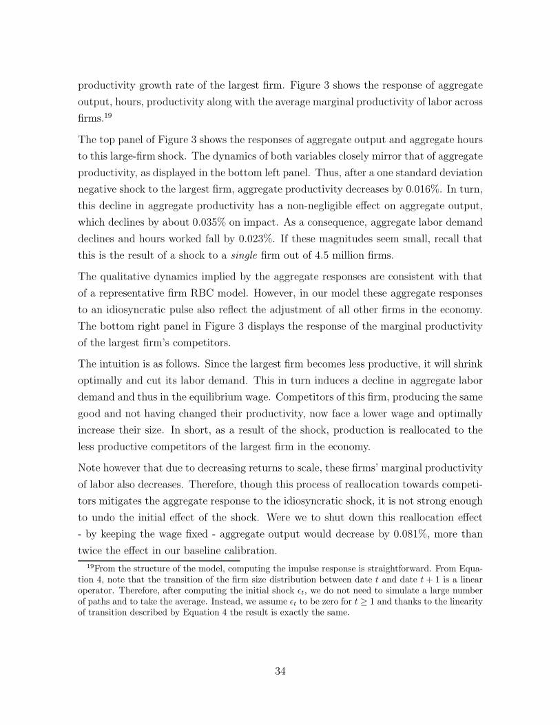
productivity growth rate of the largest firm. Figure 3 shows the response of aggregate

output, hours, productivity along with the average marginal productivity of labor across

firms.19

The top panel of Figure 3 shows the responses of aggregate output and aggregate hours

to this large-firm shock. The dynamics of both variables closely mirror that of aggregate

productivity, as displayed in the bottom left panel. Thus, after a one standard deviation

negative shock to the largest firm, aggregate productivity decreases by 0.016%. In turn,

this decline in aggregate productivity has a non-negligible effect on aggregate output,

which declines by about 0.035% on impact. As a consequence, aggregate labor demand

declines and hours worked fall by 0.023%. If these magnitudes seem small, recall that

this is the result of a shock to a single firm out of 4.5 million firms.

The qualitative dynamics implied by the aggregate responses are consistent with that

of a representative firm RBC model. However, in our model these aggregate responses

to an idiosyncratic pulse also reflect the adjustment of all other firms in the economy.

The bottom right panel in Figure 3 displays the response of the marginal productivity

of the largest firm’s competitors.

The intuition is as follows. Since the largest firm becomes less productive, it will shrink

optimally and cut its labor demand. This in turn induces a decline in aggregate labor

demand and thus in the equilibrium wage. Competitors of this firm, producing the same

good and not having changed their productivity, now face a lower wage and optimally

increase their size. In short, as a result of the shock, production is reallocated to the

less productive competitors of the largest firm in the economy.

Note however that due to decreasing returns to scale, these firms’ marginal productivity

of labor also decreases. Therefore, though this process of reallocation towards competi-

tors mitigates the aggregate response to the idiosyncratic shock, it is not strong enough

to undo the initial effect of the shock. Were we to shut down this reallocation effect

- by keeping the wage fixed - aggregate output would decrease by 0.081%, more than

twice the effect in our baseline calibration.19From the structure of the model, computing the impulse response is straightforward. From Equa-

tion 4, note that the transition of the firm size distribution between date t and date t + 1 is a linearoperator. Therefore, after computing the initial shock ϵt, we do not need to simulate a large numberof paths and to take the average. Instead, we assume ϵt to be zero for t ≥ 1 and thanks to the linearityof transition described by Equation 4 the result is exactly the same.

34

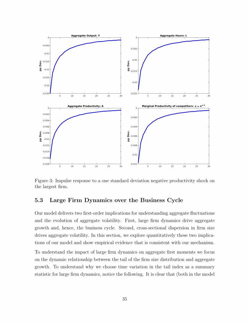
5 10 15 20 25 30

pp D

ev.

-0.035

-0.03

-0.025

-0.02

-0.015

-0.01

-0.005

0Aggregate Output: Y

5 10 15 20 25 30

pp D

ev.

-0.025

-0.02

-0.015

-0.01

-0.005

0Aggregate Hours: L

5 10 15 20 25 30

pp D

ev.

-0.018

-0.016

-0.014

-0.012

-0.01

-0.008

-0.006

-0.004

-0.002

0Aggregate Productivity: A

Figure 3: Impulse response to a one standard deviation negative productivity shock onthe largest firm.

5.3 Large Firm Dynamics over the Business Cycle

Our model delivers two first-order implications for understanding aggregate fluctuations

and the evolution of aggregate volatility. First, large firm dynamics drive aggregate

growth and, hence, the business cycle. Second, cross-sectional dispersion in firm size

drives aggregate volatility. In this section, we explore quantitatively these two implica-

tions of our model and show empirical evidence that is consistent with our mechanism.

To understand the impact of large firm dynamics on aggregate first moments we focus

on the dynamic relationship between the tail of the firm size distribution and aggregate

growth. To understand why we choose time variation in the tail index as a summary

statistic for large firm dynamics, notice the following. It is clear that (both in the model

35

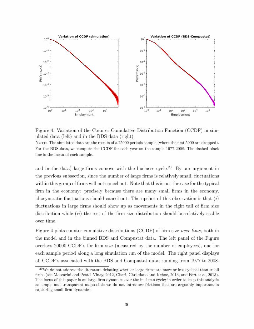
Employment100 101 102 103 104

Pr(rm

s>x)

10-6

10-5

10-4

10-3

10-2

10-1

100Variation of CCDF (simulation)

—– Employment100 101 102 103 104 105

Pr(firm

s>x)

10-6

10-5

10-4

10-3

10-2

10-1

100Variation of CCDF (BDS-Compustat)

Figure 4: Variation of the Counter Cumulative Distribution Function (CCDF) in sim-ulated data (left) and in the BDS data (right).Note: The simulated data are the results of a 25000 periods sample (where the first 5000 are dropped).

For the BDS data, we compute the CCDF for each year on the sample 1977-2008. The dashed black

line is the mean of each sample.

and in the data) large firms comove with the business cycle.20 By our argument in

the previous subsection, since the number of large firms is relatively small, fluctuations

within this group of firms will not cancel out. Note that this is not the case for the typical

firm in the economy: precisely because there are many small firms in the economy,

idiosyncratic fluctuations should cancel out. The upshot of this observation is that (i)

fluctuations in large firms should show up as movements in the right tail of firm size

distribution while (ii) the rest of the firm size distribution should be relatively stable

over time.

Figure 4 plots counter-cumulative distributions (CCDF) of firm size over time, both in

the model and in the binned BDS and Compustat data. The left panel of the Figure

overlays 20000 CCDF’s for firm size (measured by the number of employees), one for

each sample period along a long simulation run of the model. The right panel displays

all CCDF’s associated with the BDS and Compustat data, running from 1977 to 2008.

20We do not address the literature debating whether large firms are more or less cyclical than smallfirms (see Moscarini and Postel-Vinay, 2012, Chari, Christiano and Kehoe, 2013, and Fort et al, 2013).The focus of this paper is on large firm dynamics over the business cycle; in order to keep this analysisas simple and transparent as possible we do not introduce frictions that are arguably important incapturing small firm dynamics.

36

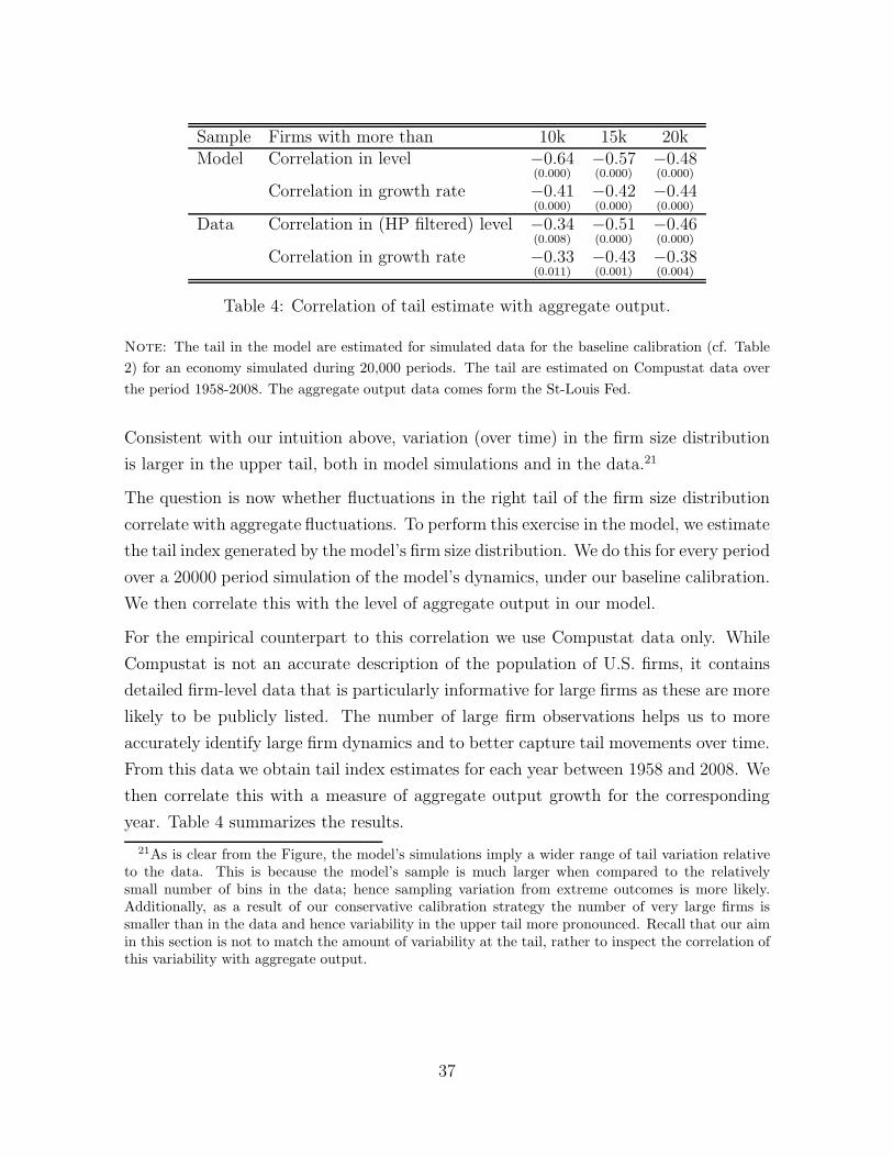
Sample Firms with more than 10k 15k 20kModel Correlation in level −0.64

(0.000)−0.57(0.000)

−0.48(0.000)

Correlation in growth rate −0.41(0.000)

−0.42(0.000)

−0.44(0.000)

Data Correlation in (HP filtered) level −0.34(0.008)

−0.51(0.000)

−0.46(0.000)

Correlation in growth rate −0.33(0.011)

−0.43(0.001)

−0.38(0.004)

Table 4: Correlation of tail estimate with aggregate output.

Note: The tail in the model are estimated for simulated data for the baseline calibration (cf. Table

2) for an economy simulated during 20,000 periods. The tail are estimated on Compustat data over

the period 1958-2008. The aggregate output data comes form the St-Louis Fed.

Consistent with our intuition above, variation (over time) in the firm size distribution

is larger in the upper tail, both in model simulations and in the data.21

The question is now whether fluctuations in the right tail of the firm size distribution

correlate with aggregate fluctuations. To perform this exercise in the model, we estimate

the tail index generated by the model’s firm size distribution. We do this for every period

over a 20000 period simulation of the model’s dynamics, under our baseline calibration.

We then correlate this with the level of aggregate output in our model.

For the empirical counterpart to this correlation we use Compustat data only. While

Compustat is not an accurate description of the population of U.S. firms, it contains

detailed firm-level data that is particularly informative for large firms as these are more

likely to be publicly listed. The number of large firm observations helps us to more

accurately identify large firm dynamics and to better capture tail movements over time.

From this data we obtain tail index estimates for each year between 1958 and 2008. We

then correlate this with a measure of aggregate output growth for the corresponding

year. Table 4 summarizes the results.

21As is clear from the Figure, the model’s simulations imply a wider range of tail variation relativeto the data. This is because the model’s sample is much larger when compared to the relativelysmall number of bins in the data; hence sampling variation from extreme outcomes is more likely.Additionally, as a result of our conservative calibration strategy the number of very large firms issmaller than in the data and hence variability in the upper tail more pronounced. Recall that our aimin this section is not to match the amount of variability at the tail, rather to inspect the correlation ofthis variability with aggregate output.

37

For our baseline case, we choose to estimate tail indexes based on information for

firms with more than 10000 employees, both in the model and in the data.22. The

correlation between the tail estimate and the level of aggregate output in the model is

negative (-0.64) and significant. The corresponding exercise in the data correlates the

HP filtered aggregate output series and correlates this with the tail indexes estimated

from Compustat. This correlation is again negative (-0.34) and significant. Intuitively,

in periods when large firms suffer negative shocks, the tail index estimate is larger, i.e.

the firm size distribution is less fat tailed. Both in the model and in the data, these

periods coincide with below-trend performance at the aggregate level.

The remaining columns in the Table 4 present different robustness checks. First, we

assess whether our results are sensitive to the cutoff choice when estimating tails. To

do this, we re-estimate the empirical tail series in Compustat using larger scale cutoffs.

The results are, if anything, stronger: the more we focus on the behavior of very large

firms the stronger is the correlation in the data.23 Our second robustness check, assesses

whether this correlation survives a growth rate specification. The correlation between

tail indices and aggregate output growth is again negative and does not depend on the

particular cutoff chosen for the tail estimation.

Our model also has implications for the evolution of aggregate volatility over time.

According to our discussion following Proposition 2 in the previous section, periods of

high cross-sectional dispersion in firm size are periods of high volatility in aggregate

output and aggregate TFP.

Our measure of cross-section dispersion in data is again sourced from Compustat. For

each year, we compute the variance of (the logarithm of) real sales of manufacturing

firms. We deflate the original nominal sales values in Compustat by the corresponding

industry 4-digit price deflator from the NBER-CES Manufacturing database. For a

measure of aggregate volatility, we follow Bloom et al (2014) and take the conditional

volatility estimates from a GARCH(1,1) specification on aggregate TFP growth and

aggregate GDP growth. Since both series contain low frequency movements we HP

filter each series.

To obtain the model counterpart of the conditional volatility in aggregate output we

make use of our analytical solution in Equation 11. We then correlate this series with

22For the model, we implement the estimator by Virkar and Clauset (2014) with a fixed cutoff. Forthe Compustat data, we follow Gabaix and Ibragimov (2011)

23In the Data Appendix we also show that this is robust to considering smaller cutoffs.

38

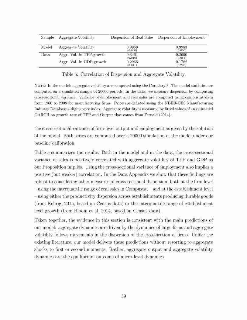
Sample Aggregate Volatility Dispersion of Real Sales Dispersion of Employment

Model Aggregate Volatility 0.9968(0.000)

0.9983(0.000)

Data Aggr. Vol. in TFP growth 0.3461(0.016)

0.2690(0.065)

Aggr. Vol. in GDP growth 0.2966(0.041)

0.1782(0.226)

Table 5: Correlation of Dispersion and Aggregate Volatility.

Note: In the model: aggregate volatility are computed using the Corollary 3. The model statistics are

computed on a simulated sample of 20000 periods. In the data: we measure dispersion by computing

cross-sectional variance. Variance of employment and real sales are computed using compustat data

from 1960 to 2008 for manufacturing firms. Price are deflated using the NBER-CES Manufacturing

Industry Database 4-digits price index. Aggregate volatility is measured by fitted values of an estimated

GARCH on growth rate of TFP and Output that comes from Fernald (2014).

the cross-sectional variance of firm-level output and employment as given by the solution

of the model. Both series are computed over a 20000 simulation of the model under our

baseline calibration.

Table 5 summarizes the results. Both in the model and in the data, the cross-sectional

variance of sales is positively correlated with aggregate volatility of TFP and GDP as

our Proposition implies. Using the cross-sectional variance of employment also implies a

positive (but weaker) correlation. In the Data Appendix we show that these findings are

robust to considering other measures of cross-sectional dispersion, both at the firm level

– using the interquartile range of real sales in Compustat – and at the establishment level

– using either the productivity dispersion across establishments producing durable goods

(from Kehrig, 2015, based on Census data) or the interquartile range of establishment

level growth (from Bloom et al, 2014, based on Census data).

Taken together, the evidence in this section is consistent with the main predictions of

our model: aggregate dynamics are driven by the dynamics of large firms and aggregate

volatility follows movements in the dispersion of the cross-section of firms. Unlike the

existing literature, our model delivers these predictions without resorting to aggregate

shocks to first or second moments. Rather, aggregate output and aggregate volatility

dynamics are the equilibrium outcome of micro-level dynamics.

39

5.4 Distributional Dynamics and the Business Cycle

The core of our argument is that the firm size distribution is a “sufficient statistic”

for understanding fluctuations in aggregates. The aggregate state in our model is the

firm size distribution. The evolution of this object over time determines aggregate

output and its volatility. In the quantitative exercises above we have shown that certain

moments of this distribution – its maximum in the impulse response analysis exercise

and its tail and cross-sectional second moment in the previous subsection – do influence

aggregates and that their quantitative impact is non-negligible.

In this section, we take this “sufficient statistic” argument one step further. Suppose we

had access to a single time series object – the evolution of the firm size distribution over

time as given by the BDS data. Using our calibrated model as an aggregation device we

ask: what would be the implied history of aggregate fluctuations and volatility, based

on this data alone?

To do this we use the expressions that aggregate the information in the firm size dis-

tribution and deliver aggregate productivity (Equation 1), aggregate output (Equation

3) and aggregate volatility (Equation 11) in the model.24 As a result of this exercise,

we obtain from our model three aggregate time series - for aggregate output, aggre-

gate productivity and the volatility of aggregate output - whose time variation reflects

movements in the size distribution over time alone. Figure 5 plots these three series

(solid lines) against their HP filtered data counterparts (dashed lines).

As Figure 5 renders clear, when interpreted through the lenses of our model, the em-

pirical evolution of the firm size distribution implies aggregate fluctuations that track

well the historical fluctuations in aggregate data. In all three cases, the correlation

between the implied and actual aggregates is positive and statistically significant. The

estimates implied by the firm size distribution data track the evolution of aggregate

24To feed these expressions with data on the firm size distribution we must additionally resolve oneissue: the model takes as a primitives the productivity grid Φ. Instead, the data on the firm sizedistribution by the BDS takes as primitives the bins of the firm size, which are fixed over time. Thus,given a size distribution at time t, we need to solve for the productivity bins in our model that areconsistent with the observed size distribution. This can be easily obtained by using the optimalitycondition with respect to employment and the labor market clearing condition. To be precise, denotethe information in the data by nBDS

s , the observed number of firms with employment in bin s. We then

solve for the productivity grid ΦBDSt and wage rate wBDS

t such that (i)∀s, ϕBDSs,t = wBDS

tα (nBDS

s )1−α

and (ii)wBDSt =

(α

11−α

∑SBDS

s=1 (ϕBDSs,t )

11−α µBDS

s,t

M

) 1−αγ(1−α)+1

.

40

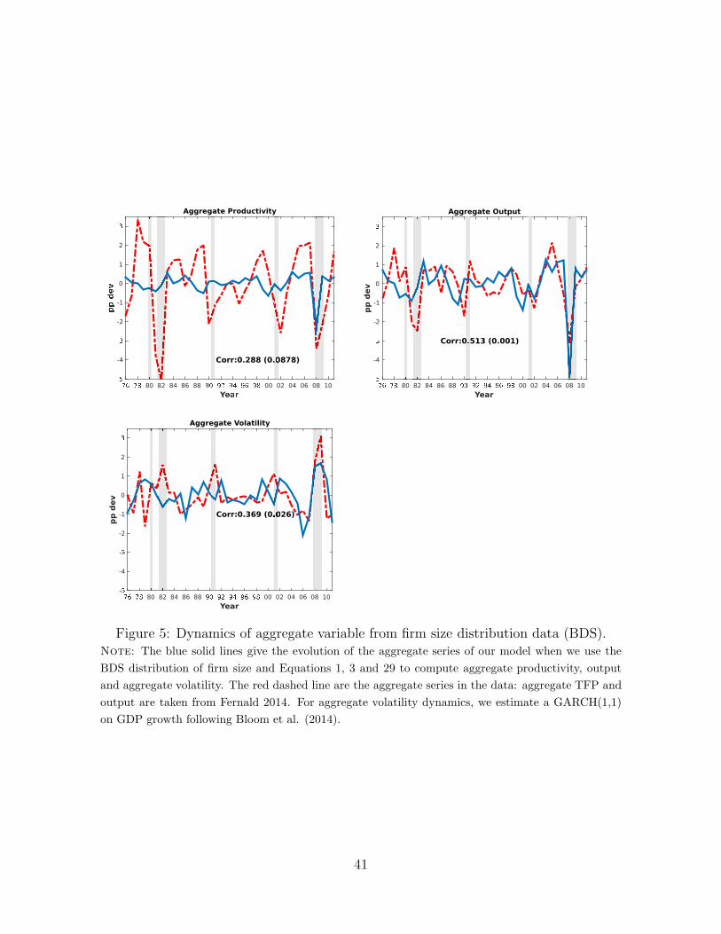
Y80 82 84 86 88 00 02 04 06 08 10

-4

-2

-1

0

1

2

Corr:0.288 (0.0878)

Aggregate Productivity

Year80 82 84 86 88 00 02 04 06 08 10

pp d

ev-4

-2

-1

0

1

2

Corr:0.513 (0.001)

Aggregate Output

Year80 82 84 86 88 00 02 04 06 08 10

pp d

ev

-4

-2

-1

0

1

2

Corr:0.369 (0.026)

Aggregate Volatility

Figure 5: Dynamics of aggregate variable from firm size distribution data (BDS).Note: The blue solid lines give the evolution of the aggregate series of our model when we use the

BDS distribution of firm size and Equations 1, 3 and 29 to compute aggregate productivity, output

and aggregate volatility. The red dashed line are the aggregate series in the data: aggregate TFP and

output are taken from Fernald 2014. For aggregate volatility dynamics, we estimate a GARCH(1,1)

on GDP growth following Bloom et al. (2014).

41

output (in deviations from trend) particularly well with a highly significant correlation

of 0.533. For aggregate productivity and the conditional volatility of aggregate TFP,

this correlation is about 1/3 and noisier, which mostly reflects a weaker correlation in

the earlier part of the sample. Conversely, the data on the firm size distribution implies

remarkably accurate aggregate dynamics in the period leading up to, during and after

the Great Recession.

In summary, coupling the information contained in the dynamics of the firm size dis-

tribution with our quantitative model delivers a history of aggregate fluctuations that

is not unlike what we observe in the aggregate data.

6 Conclusion

A small number of firms accounts for a substantial share of aggregate economic activity.

This opens the possibility of doing away with aggregate shocks, instead tracing back

the origins of aggregate fluctuations to large firm dynamics. We build a quantitative

firm dynamics model in which we cast this hypothesis.

The first part of our analysis characterizes, analytically, the law of motion of the firm size

distribution and shows that the implied aggregate output and productivity dynamics

are persistent, volatile and exhibit time-varying second moments.

In the second part of the paper, we explore quantitatively and in the data, the role

of the firm size distribution – and, in particular, that of large firm dynamics – in

shaping aggregate fluctuations. Taken together, our results imply that a large fraction

of aggregate dynamics can be rationalized by large firm dynamics.

The results in this paper suggest at least two fruitful ways of extending our analysis.

First, while we have intentionally focused our attention on large firm dynamics as drivers

of aggregate fluctuations, a complete analysis of firm dynamics over the business cycle

should also match those of small firms. This surely implies moving away from the

frictionless environment presented here and understanding how small firm dynamics

are distorted by adjustment costs, credit constraints and other frictions. The fact that

Hopenhayn’s (1992) framework is tractable enough to handle such frictions, render our

analysis easily extensible to such environments.

42

Second, in our framework, a firm does not internalize its own effect on aggregate prices

and factor costs. In other models of firms dynamics, the assumption that the law of

large numbers holds, justifies thinking about firms as infinitesimal price takers. How-

ever, we have shown that, in a standard firm dynamics framework, large firms have a

non-negligible effect on aggregates. Thus, the price taker assumption should be taken

carefully. This points to generalizations of our setup that do away with this assumption

and take on market structure and market power as further determinants of aggregate

dynamics.

43

References

[1] Daron Acemoglu, Vasco M. Carvalho, Asuman Ozdaglar, and Alireza Tahbaz-Salehi.The network origins of aggregate fluctuations. Econometrica, 80(5):1977–2016, 09 2012.

[2] Daron Acemoglu and Martin K. Jensen. Robust comparative statics in large dynamiceconomies. Journal of Political Economy, Forthcoming, 2015.

[3] Robert L. Axtell. Zipf distribution of u.s. firm sizes,. Science 7, 293(5536):1818–1820,September 2001.

[4] Susanto Basu and John G Fernald. Returns to scale in u.s. production: Estimates andimplications. Journal of Political Economy, 105(2):249–83, April 1997.

[5] Florin O. Bilbiie, Fabio Ghironi, and Marc J. Melitz. Endogenous entry, product variety,and business cycles. Journal of Political Economy, 120(2):304 – 345, 2012.

[6] Nicholas Bloom, Max Floetotto, Nir Jaimovich, Itay Saporta-Eksten, and Stephen J.Terry. Really Uncertain Business Cycles. Working Papers 14-18, Center for EconomicStudies, U.S. Census Bureau, March 2014.

[7] Jeffrey R. Campbell. Entry, exit, embodied technology, and business cycles. Review ofEconomic Dynamics, 1(2):371–408, April 1998.

[8] Jeffrey R. Campbell and Jonas D.M. Fisher. Idiosyncratic risk and aggregate employmentdynamics. Review of Economic Dynamics, 7(2):331 – 353, 2004.

[9] Vasco Carvalho and Xavier Gabaix. The Great Diversification and Its Undoing. Amer-ican Economic Review, 103(5):1697–1727, August 2013.

[10] Rui Castro, Gian Luca Clementi, and Yoonsoo Lee. Cross-sectoral variation in firm-levelidiosyncratic risk. Journal of Industrial Economics, Forthcoming.

[11] David G. Champernowne. A model of income distribution. Economic Journal,63(250):318–351, June 1953.

[12] Varadarajan V. Chari, Lawrence J. Christiano, and Patrick J. Kehoe. The gertler-gilchrist evidence on small and large firm sales. mimeo, July 2013.

[13] Gian Luca Clementi and Berardino Palazzo. Entry, exit, firm dynamics, and aggregatefluctuations. Working Paper 19217, National Bureau of Economic Research, July 2015.

[14] Gina Luca Clementi and Hugo A Hopenhayn. A Theory of Financing Constraints andFirm Dynamics. The Quarterly Journal of Economics, 121(1):229–265, 02 2006.

[15] Diego A. Comin and Thomas Philippon. The rise in firm-level volatility: Causes andconsequences. In NBER Macroeconomics Annual 2005, Volume 20, NBER Chapters,pages 167–228. National Bureau of Economic Research, Inc, October 2006.

[16] Juan Carlos Cordoba. A generalized gibrat’s law. International Economic Review,49(4):1463–1468, November 2008.

44

[17] Steven J. Davis, John Haltiwanger, Ron Jarmin, and Javier Miranda. Volatility andDispersion in Business Growth Rates: Publicly Traded versus Privately Held Firms.In NBER Macroeconomics Annual 2006, Volume 21, NBER Chapters, pages 107–180.National Bureau of Economic Research, Inc, October 2007.

[18] Wouter J. Den Haan and Pontus Rendahl. Solving the incomplete markets model withaggregate uncertainty using explicit aggregation. Journal of Economic Dynamics andControl, 34(1):69–78, January 2010.

[19] Julian di Giovanni and Andrei A. Levchenko. Country size, international trade, andaggregate fluctuations in granular economies. Journal of Political Economy, 120(6):1083– 1132, 2012.

[20] Julian di Giovanni, Andrei A. Levchenko, and Isabelle Mejean. Firms, Destinations, andAggregate Fluctuations. Econometrica, 82(4):1303–1340, 07 2014.

[21] Julian di Giovanni, Andrei A. Levchenko, and Isabelle Mejean. Granular comovment.Technical report, December 2014.

[22] Timothy Dunne, Mark J. Roberts, and Larry Samuelson. Patterns of firm entry and exitin u.s. manufacturing industries. The RAND Journal of Economics, 19(4):pp. 495–515,1988.

[23] David S Evans. The Relationship between Firm Growth, Size, and Age: Estimatesfor 100 Manufacturing Industries. Journal of Industrial Economics, 35(4):567–81, June1987.

[24] John Fernald. A quarterly, utilization-adjusted series on total factor productivity. Work-ing Paper Series 2012-19, Federal Reserve Bank of San Francisco, 2014.

[25] Teresa C Fort, John Haltiwanger, Ron S Jarmin, and Javier Miranda. How FirmsRespond to Business Cycles: The Role of Firm Age and Firm Size. IMF EconomicReview, 61(3):520–559, August 2013.

[26] Lucia Foster, John Haltiwanger, and Chad Syverson. Reallocation, Firm Turnover, andEfficiency: Selection on Productivity or Profitability? American Economic Review,98(1):394–425, March 2008.

[27] Xavier Gabaix. The granular origins of aggregate fluctuations. Econometrica, 79(3):733–772, 05 2011.

[28] Xavier Gabaix and Rustam Ibragimov. Rank-1/2: A Simple Way to Improve the OLSEstimation of Tail Exponents. Journal of Business & Economic Statistics, 29(1):24–39,2011.

[29] Bronwyn H Hall. The Relationship between Firm Size and Firm Growth in the U.S.Manufacturing Sector. Journal of Industrial Economics, 35(4):583–606, June 1987.

[30] Hugo A Hopenhayn. Entry, exit, and firm dynamics in long run equilibrium. Economet-rica, 60(5):1127–50, September 1992.

[31] JPMorgan. Can one little phone impact gdp? Michael Feroli, North AmericaEconomic Research, https://mm.jpmorgan.com/EmailPubServlet?doc=GPS-938711-0.html&h=-825pgod, 2012.

45

[32] Matthias Kehrig. The cyclical nature of the productivity distribution. January 2015.

[33] Aubhik Khan and Julia K. Thomas. Idiosyncratic shocks and the role of nonconvexitiesin plant and aggregate investment dynamics. Econometrica, 76(2):395–436, 03 2008.

[34] Per Krusell and Anthony A. Smith. Income and wealth heterogeneity in the macroecon-omy. Journal of Political Economy, 106(5):867–896, October 1998.

[35] Yoonsoo Lee. The importance of reallocations in cyclical productivity and returns toscale: evidence from plant-level data. Working Paper 0509, Federal Reserve Bank ofCleveland, 2005.

[36] Yoonsoo Lee and Toshihiko Mukoyama. Entry, exit and plant-level dynamics over thebusiness cycle. Working Paper 0718, Federal Reserve Bank of Cleveland, 2008.

[37] Erzo G. J. Luttmer. Selection, growth, and the size distribution of firms. The QuarterlyJournal of Economics, 122(3):1103–1144, 08 2007.

[38] Erzo G.J. Luttmer. Models of growth and firm heterogeneity. Annual Review of Eco-nomics, 2(1):547–576, 09 2010.

[39] Erzo G.J. Luttmer. Technology diffusion and growth. Journal of Economic Theory,147(2):602–622, 2012.

[40] Mario J. Miranda and Paul L. Fackler. Applied Computational Economics and Finance,volume 1 of MIT Press Books. The MIT Press, June 2004.

[41] Giuseppe Moscarini and Fabien Postel-Vinay. The contribution of large and small em-ployers to job creation in times of high and low unemployment. American EconomicReview, 102(6):2509–39, October 2012.

[42] Mark E. J. Newman. Power laws, pareto distributions and zipf’s law. ContemporaryPhysics, 46:323–351, 2005.

[43] Richard Rogerson and Johanna Wallenius. Micro and macro elasticities in a life cyclemodel with taxes. Journal of Economic Theory, 144(6):2277–2292, November 2009.

[44] Esteban Rossi-Hansberg and Mark L. J. Wright. Establishment Size Dynamics in theAggregate Economy. American Economic Review, 97(5):1639–1666, December 2007.

[45] Herbert A. Simon. On a class of skew distribution functions. Biometrika, 42(3-4):425–440, 1955.

[46] Chad Syverson. Product Substitutability and Productivity Dispersion. The Review ofEconomics and Statistics, 86(2):534–550, May 2004.

[47] Marcelo L. Veracierto. Plant-level irreversible investment and equilibrium business cy-cles. American Economic Review, 92(1):181–197, March 2002.

[48] Yogesh Virkar and Aaron Clauset. Power-law distributions in binned empirical data.Annals of Applied Statistics, 8(1):89–119, 2014.

46

Online Appendix to “Large Firm Dynamics and the BusinessCycle”

Vasco M. Carvalho and Basile Grassi

Not for Publication. March 2015

A Proof Appendix

In this appendix, we first solve for the stationary distribution under random growth describedin Corollary 2 (Appendix A.1). We then find the asymptotic value of the ratio between thenumber of incumbents and the number of potential entrants, when the former goes to infinity(Appendix A.2). This intermediate result will be used in the rest of this appendix. InAppendix A.3, we prove Theorem 2 describing the dynamics of the aggregate state Tt. InAppendix A.4, we solve for the dynamics of aggregate output up to a first order approximationas in Corollary 3. Finally, in Appendix A.5 and A.6, we prove Proposition 1 and 2 containingour comparative statics’ results for aggregate persistence and volatility respectively.

A.1 Proof of Corollary 2

In this appendix, we prove that the productivity stationary distribution is a mixture oftwo distributions: (i) the stationary distribution associated with the Markovian firm-levelproductivity process and (ii) the distribution of entrants. These are respectively weighted

by the constants K1 and K2. Formally, we show that K1 = − ca

(ϕδe−1)(ϕ−δe )s∗

(1−ϕ−δe )(aϕ−δe−c) and K2 =(ϕδe−1)(a(ϕ−δe )2+bϕ−δe+c)

a(ϕ−δe )2−ϕ−δe(a+c)+c (ϕs∗)−δe . In the Corollary in the main text, we only reported the valueof the productivity stationary distribution for productivity levels above the exit threshold.In this appendix, for completeness, we describe this distribution over the full idiosyncraticstate-space. We then show that:

µs =

⎧⎪⎪⎪⎪⎪⎨

⎪⎪⎪⎪⎪⎩

− ca

(ϕδe−1)(ϕ−δe )s∗

(1−ϕ−δe )(aϕ−δe−c)

(ϕs

ϕs∗

)−δ+

(ϕδe−1)(a(ϕ−δe )2+bϕ−δe+c)a(ϕ−δe )2−ϕ−δe (a+c)+c (ϕs)−δe if s ≥ s∗

a(ϕδe − 1

) ( −c/a(1−ϕ−δe )(aϕ−δe−c) +

a(ϕ−δe )2+bϕ−δe+ca(ϕ−δe )2−(a+c)ϕ−δe+c + 1

)(ϕs∗)−δe if i = s∗ − 1

0 if s < s∗ − 1

with δ = log(a/c)log(ϕ) .

The proof of this Corollary follows two steps: (i) we first solve closed-form for the stationarydistribution given a maximum level of productivity ϕS under Assumption 1; (ii) we then takethe limit of this distribution when the number of firms goes to infinity under the Assumption2.Step 1: for a given S and a given number of firms

This step consists of solving for the stationary distribution given a fixed maximum level ofproductivity S. Formally, in this step, we will show that the following Lemma holds true.

47

Lemma 1 For a given S, if (i) the entrant distribution is Pareto (i.e Gs = Ke (ϕs)−δe) and(ii) the productivity process follows Gibrat’s law (Assumption 1) with parameters a and c onthe grid defined by ϕ, then the stationary distribution (i.e when Vartϵt+1 = 0) is:

For s∗ ≤ s ≤ S:

µs = P{ϕ = ϕs} = MKeC1

(ϕs

ϕs∗

)−δ

+MKeC2 (ϕs)−δe +MKeC3

and µs∗−1 = a(µs∗ +MKe

(ϕs∗)−δe

)and µs = 0 for s < s∗ − 1.

Where δ = log(a/c)log(ϕ) and C1, C2, C3 are constants, independent of s, and where

C1 =c(a(ϕ−δe )S+2−a(ϕ−δe )s

∗

−c(ϕ−δe )S+3+c(ϕ−δe)s∗)

a(1−ϕ−δe )(a−c)(aϕ−δe−c) , C2 =(a(ϕ−δe )2+bϕ−δe+c)

(a(ϕ−δe )2−ϕ−δe(a+c)+c) and C3 =−(ϕ−δe )S+1

(1−ϕ−δe )(a−c) .

Proof: To find the stationary distribution of the Markovian process described by the transi-tion matrix P , we need to solve for µ in µ = (P ∗

t )′(µ+MG) where P is given by assumption

1 and where µ is the (S × 1) vector (µ1, . . . , µS)′. For simplicity, we assume M = 1.

The matrix Equation µ = (P ∗t )

′(µ+MG) can be equivalently written as the following systemof Equations:

For s < s∗ − 1:µs = 0 (14)

For s = s∗ − 1:µs∗−1 = a(µs∗ +Gs∗) (15)

For s = s∗:µs∗ = b(µs∗ +Gs∗) + a(µs∗+1 +Gs∗+1) (16)

For s = S:µS = c(µS−1 +GS−1) + (b+ c)(µS +GS) (17)

For s∗ + 1 ≤ s ≤ S − 1:

µs = c(µs−1 +Gs−1) + b(µs +Gs) + a(µs+1 +Gs+1) (18)

The system of Equations 16, 17 and 18 gives a linear second difference Equation with twoboundary conditions. The system has a exogenous term given by the distribution of entrantsG. For this system, we define the associated homogeneous system by the same Equations withGs = 0,∀s. To solve for a linear second order difference Equation, we follow four steps: (i)Solve for the general solution of the homogeneous system; these solutions are parametrized bytwo constants (ii) Find one particular solution for the full system (iii) The general solutionof the full system is then given by the sum of the general solution of the homogeneous systemand the particular solution we have found (iv) Solve for the undetermined coefficient usingthe boundary conditions.

The recurrence Equation of the homogeneous system is equivalent to cµs−1 − (a + c)µs +aµs+1 = 0 since b = 1 − a − c. To find the general solution of this Equation, let us solve forthe root of the polynomial aX2− (a+ c)X+ c. This polynomial is equal to a(X− c/a)(X−1)and thus its roots are r1 = c/a and 1. The general solution of the homogeneous systemassociated to Equation 18 is then µs = A(c/a)s +B where A and B are constants.

Using the form of the entrant distribution Gs = Ke(ϕ−δe)s, and assuming that ϕ−δe = ac , a

particular solution is Kea(ϕ−δe )2+bϕ−δe+c

a(ϕ−δe )2−(a+c)ϕ−δe+c(ϕ−δe)s.

48

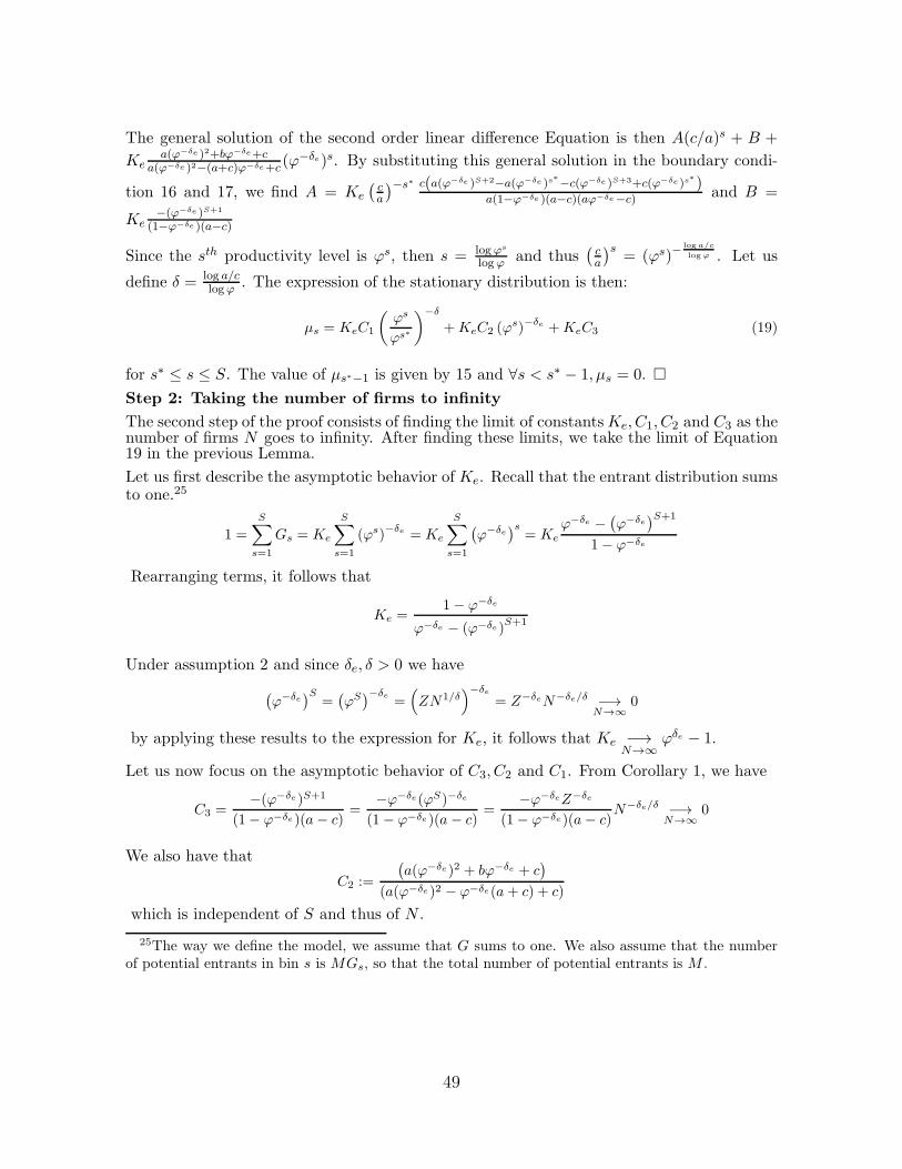
The general solution of the second order linear difference Equation is then A(c/a)s + B +

Kea(ϕ−δe )2+bϕ−δe+c

a(ϕ−δe )2−(a+c)ϕ−δe+c(ϕ−δe)s. By substituting this general solution in the boundary condi-

tion 16 and 17, we find A = Ke(ca

)−s∗ c(a(ϕ−δe )S+2−a(ϕ−δe )s∗

−c(ϕ−δe )S+3+c(ϕ−δe)s∗)

a(1−ϕ−δe )(a−c)(aϕ−δe−c) and B =

Ke−(ϕ−δe )S+1

(1−ϕ−δe )(a−c)

Since the sth productivity level is ϕs, then s = logϕs

logϕ and thus(ca

)s= (ϕs)−

log a/c

log ϕ . Let us

define δ = log a/clogϕ . The expression of the stationary distribution is then:

µs = KeC1

(ϕs

ϕs∗

)−δ

+KeC2 (ϕs)−δe +KeC3 (19)

for s∗ ≤ s ≤ S. The value of µs∗−1 is given by 15 and ∀s < s∗ − 1, µs = 0. !

Step 2: Taking the number of firms to infinity

The second step of the proof consists of finding the limit of constantsKe, C1, C2 and C3 as thenumber of firms N goes to infinity. After finding these limits, we take the limit of Equation19 in the previous Lemma.

Let us first describe the asymptotic behavior of Ke. Recall that the entrant distribution sumsto one.25

1 =S∑

s=1

Gs = Ke

S∑

s=1

(ϕs)−δe = Ke

S∑

s=1

(ϕ−δe

)s= Ke

ϕ−δe −(ϕ−δe

)S+1

1− ϕ−δe

Rearranging terms, it follows that

Ke =1− ϕ−δe

ϕ−δe − (ϕ−δe)S+1

Under assumption 2 and since δe, δ > 0 we have

(ϕ−δe

)S=(ϕS)−δe

=(ZN1/δ

)−δe= Z−δeN−δe/δ −→

N→∞0

by applying these results to the expression for Ke, it follows that Ke −→N→∞

ϕδe − 1.

Let us now focus on the asymptotic behavior of C3, C2 and C1. From Corollary 1, we have

C3 =−(ϕ−δe)S+1

(1− ϕ−δe)(a− c)=

−ϕ−δe(ϕS)−δe

(1− ϕ−δe)(a− c)=

−ϕ−δeZ−δe

(1− ϕ−δe)(a− c)N−δe/δ −→

N→∞0

We also have that

C2 :=

(a(ϕ−δe)2 + bϕ−δe + c

)

(a(ϕ−δe)2 − ϕ−δe(a+ c) + c)

which is independent of S and thus of N .

25The way we define the model, we assume that G sums to one. We also assume that the numberof potential entrants in bin s is MGs, so that the total number of potential entrants is M .

49

Finally, we have

C1 =c(a(ϕ−δe)S+2 − a(ϕ−δe)s

∗

− c(ϕ−δe)S+3 + c(ϕ−δe)s∗)

a(1− ϕ−δe)(a− c)(aϕ−δe − c)

−→N→∞

c(−a(ϕ−δe)s

∗

+ c(ϕ−δe)s∗)

a(1− ϕ−δe)(a− c)(aϕ−δe − c)=

c

a

−(a− c)(ϕ−δe )s∗

(1− ϕ−δe)(a− c)(aϕ−δe − c)

and therefore

C1 −→N→∞

C∞1 :=

c

a

(ϕ−δe)s∗

(1− ϕ−δe)(c− aϕ−δe)

We have just found the limit of Ke, C1, C2 and C3 when N goes to infinity. We then applythese results to the stationary distribution by taking N to infinity. According to Lemma 1,we have for s∗ ≤ s ≤ S:

µs

M= KeC1

(ϕs

ϕs∗

)−δ

+KeC2(ϕs)−δe +KeC3

Under assumption 2, we have just shown that when the number of firms, N , goes to infinity,the stationary distribution is given by:

µs

M=(ϕδe − 1

) ca

(ϕ−δe)s∗

(1− ϕ−δe)(c− aϕ−δe)

(ϕs

ϕs∗

)−δ

+(ϕδe − 1

)(a(ϕ−δe)2 + bϕ−δe + c

)

(a(ϕ−δe)2 − ϕ−δe(a+ c) + c)(ϕs)−δe

!

A.2 Intermediate result: the link between the number of in-cumbents N and the number of potential entrants M

In this appendix, we are interested in the relationship between the number of incumbents N ,the number of potentials entrantsM , and the value of their ratio when N goes to infinity. Weshow that as N goes to infinity, the ratio M/N goes to a constant. This means that takingthe endogenous variable N or the exogenous parameter M to infinity is strictly equivalent.

The number of firms is simply the sum of the number of firms in each bin:

N =S∑

s=1

µs = µs∗−1 +S∑

s=s∗

µs

=a(MKeC1 +MKeC2(ϕ

s∗)−δe +MKeC3 +MKe(ϕs∗)−δe

)+MKeC3

S∑

s=s∗

1

+MKeC1(ϕs∗)δ

S∑

s=s∗

(ϕs)−δ +MKeC2

S∑

s=s∗

(ϕs)−δe

=a(MKeC1 +MKeC2(ϕ

s∗)−δe +MKeC3 +MKe(ϕs∗)−δe

)+MKeC3(S − s∗ + 1)

+MKeC1(ϕs∗)δ

(ϕ−δ

)s∗−(ϕ−δ

)S

1− ϕ−δ+MKeC2

(ϕ−δe

)s∗−(ϕ−δe

)S

1− ϕ−δe

thus, by dividing both side by M , we have

N

M= a

!

KeC1 +Ke(C2 + 1)(ϕs∗ )−δe +KeC3

"

+KeC3(S−s∗+1)+KeC1(ϕs∗ )δ

#

ϕ−δ$s∗

−#

ϕ−δ$S

1− ϕ−δ+KeC2

#

ϕ−δe$s∗

−#

ϕ−δe$S

1− ϕ−δe

50

Let us note that under assumption 2

(ϕ−δ

)S=(ϕS)−δ

=(ZN1/δ

)−δ= Z−δN−1 −→

N→∞0

and that, since S = 1logϕ(logZ + 1

δ logN), we have

SC3 =1

logϕ(logZ +

1

δlogN)

−ϕ−δeZ−δe

(1 − ϕ−δe)(a− c)N−δe/δ −→

N→∞0

Thus, we have that

N

M−→N→∞

(E∞)−1 :=a((ϕδe − 1)C∞

1 + (ϕδe − 1)(C2 + 1)(ϕs∗)−δe)

+ (ϕδe − 1)C∞1

1

1− ϕ−δ+ (ϕδe − 1)C2

(ϕ−δe

)s∗

1− ϕ−δe

where E∞ is the ratio of the number of potential entrants M and the number of incumbents,when there is an infinite number of incumbents. The last Equation shows that M and N areequivalent when the number of incumbents is large. Thus, taking N to infinity is the sameas taking M to infinity i.e M ∼

N→∞E∞N .

A.3 Proof of Theorem 2

In this appendix, we prove Theorem 2. To do so, we use Theorem 1, where we have µt+1 =(P ∗

t )′(µt +MG) + ϵt+1. We are interested in the law of motion of Tt = B′µt where B = {bi}i

is a vector with bi = (ϕ1

1−α )i. This law of motion is derived directly from the law of motion ofthe productivity distribution described in Theorem 1. To prove Theorem 2, we then proceedin two steps. First, we show that EtTt+1 is a function of Tt and the primitives of the model.Second, we solve for the conditional variance of Tt+1.

Formally, we assume that idiosyncratic productivities follow Gibrat’s law (Assumption 1).We also assume that G, the distribution of potential entrants, is Pareto distributed with tailindex δe, i.e we have Gs = Ke(ϕ−δe)s. In the first step, we show the following Equation forthe law of motion of Tt:

Tt+1 =ρTt main dynamics

+ ρMKe(ϕ−δeϕ

11−α )S+1 − (ϕ−δeϕ

11−α )st

(ϕ−δeϕ1

1−α )− 1contribution of entrant

− ρ(ϕ1

1−α )st−1µst−1,t contribution of exit

− c(ϕ1

1−α − 1)(ϕ1

1−α )SµS,t − c(ϕ1

1−α − 1)M(ϕ−δeϕ1

1−α )S upper reflecting barrier

+ σtεt+1 aggregate uncertainty (20)

where E[εt+1] = 0, Var[εt+1] = 1 and ρ = aϕ−1/(1−α) + b+ cϕ1/(1−α).

51

The second step consists in finding an expression for the conditional variance of Tt+1. Weshow that the time-varying volatility σ2

t is:

σ2t = Vart[B

′ϵt+1] =ϱDt

+ ϱMKe(ϕ−δeϕ

21−α )S+1 − (ϕ−δeϕ

21−α )st

(ϕ−δeϕ2

1−α )− 1

− ϱ(ϕ2

1−α )st−1µst−1,t

− (ϱ− ϱ′)MKe(ϕ−δe(ϕ

11−α )2)S − (ϱ− ϱ′)(ϕ

11−α )2SµS,t (21)

where Dt =∑S

s=st−1

((ϕs)

11−α

)2µs,t, and ϱ = aϕ−2/(1−α) + b+ cϕ2/(1−α) − ρ2.

Step 1: Proof of Equation 20

Here we prove Equation 20. To do so, we first consider the term B′m(µt) = B′(P ∗t )

′(µt+MG)and express it as a function of Tt and the primitives of the model. The transition P matrix is

P =

⎛

⎜⎜⎜⎝

a+ b c 0 0 · · · · · · 0 0a b c 0 · · · · · · 0 00 a b c · · · · · · 0 0· · · · · · · · · · · · · · · · · · · · · · · ·0 0 0 0 · · · a b c0 0 0 0 · · · 0 a b+ c

⎞

⎟⎟⎟⎠

because of entry/exit we have

P ∗t =

⎛

⎜⎜⎜⎜⎜⎜⎝

0 · · · 0 0 0 · · · · · · 0 0· · · · · · · · · · · · · · · · · · · · · · · · · · ·0 · · · 0 0 0 · · · · · · 0 00 · · · 0 0 0 · · · · · · 0 00 · · · a b c · · · · · · 0 0· · · · · · · · · · · · · · · · · · · · · · · · · · ·0 · · · 0 0 0 · · · a b c0 · · · 0 0 0 · · · 0 a b+ c

⎞

⎟⎟⎟⎟⎟⎟⎠

where the first non-zero row is the row indexed by st. Let us take the transpose of this lastmatrix.

(P ∗t )

′ =

⎛

⎜⎜⎜⎜⎜⎜⎝

0 · · · 0 0 0 · · · · · · 0 0· · · · · · · · · · · · · · · · · · · · · · · · · · ·0 · · · 0 0 0 · · · · · · 0 00 · · · 0 a 0 · · · · · · 0 00 · · · 0 b a · · · · · · 0 0· · · · · · · · · · · · · · · · · · · · · · · · · · ·0 · · · 0 0 0 · · · c b a0 · · · 0 0 0 · · · 0 c b+ c

⎞

⎟⎟⎟⎟⎟⎟⎠

Now the first non-zero row is the one index by st−1. Let us look at an element of the (S×1)vector (P ∗

t )′µt.

[(P ∗t )

′µt]i =S∑

k=1

[(P ∗t )

′]i,kµk,t =

⎧⎪⎪⎨

⎪⎪⎩

0 if i < st − 1aµst,t if i = st − 1bµst,t + aµst+1,t if i = stcµi−1,t + bµi,t + aµi+1,t if st < i < ScµS−1,t + (b+ c)µS,t if i = S

Now let us pre-multiply this (S × 1) vector by the (1× S) vector B′:

52

B′(P ∗t )

′µt =S∑

i=1

bi[(P∗t )

′µt]i

=bst−1aµst,t + bst(bµst,t + aµst+1,t)

+S−1∑

i=st+1

bi(cµi−1,t + bµi,t + aµi+1,t)

+ bS(cµS−1,t + (b + c)µS,t)

Focusing on the third term of the second equality:

S−1∑

i=st+1

bi(cµi−1,t + bµi,t + aµi+1,t) = cS−1∑

i=st+1

biµi−1,t + bS−1∑

i=st+1

biµi,t + aS−1∑

i=st+1

biµi+1,t

=cS−2∑

i=st

bi+1µi,t + bS−1∑

i=st+1

biµi,t + aS∑

i=st+2

bi−1µi,t

Since bi = (ϕ1/(1−α))i then bi = ϕ1/(1−α)bi−1, we have

S−1∑

i=st+1

bi(cµi−1,t + bµi,t + aµi+1,t) =cϕ1/(1−α)S−2∑

i=st

biµi,t + bS−1∑

i=st+1

biµi,t + a(ϕ1/(1−α))−1S∑

i=st+2

biµi,t

=(c(ϕ1/(1−α)) + b+ a(ϕ1/(1−α))−1

) S−2∑

i=st+2

biµi,t

+ cϕ1/(1−α) (bstµst,t + bst+1µst+1,t)

+ b (bst+1µst+1,t + bS−1µS−1,t)

+ a(ϕ1/(1−α))−1 (bS−1µS−1,t + bSµS,t)

Introducing this term in the Equation for B′(P ∗t )

′µt yields:

B′(P ∗t )

′µt =(cϕ1/(1−α) + b+ a(ϕ1/(1−α))−1

) S−2∑

i=st+2

biµi,t

+ cϕ1/(1−α) (bstµst,t + bst+1µst+1,t)

+ b (bst+1µst+1,t + bS−1µS−1,t)

+ a(ϕ1/(1−α))−1 (bS−1µS−1,t + bSµS,t)

+ bst−1aµst,t + bst(bµst,t + aµst+1,t)

+ bS(cµS−1,t + (b + c)µS,t)

53

Rearranging terms, we have

B′(P ∗t )

′µt =(cϕ1/(1−α) + b+ a(ϕ1/(1−α))−1

) S−2∑

i=st+2

biµi,t

+ bstµst,t

(cϕ1/(1−α) + b+ a(ϕ1/(1−α))−1

)

+ bst+1µst+1,t

(cϕ1/(1−α) + b + a(ϕ1/(1−α))−1

)

+ bS−1µS−1,t

(cϕ1/(1−α) + b+ a(ϕ1/(1−α))−1

)

+ bSµS,t

((b+ c) + a(ϕ1/(1−α))−1

)

and plugging them back in the sum

B′(P ∗t )

′µt =(cϕ1/(1−α) + b+ a(ϕ1/(1−α))−1

) S−1∑

i=st

biµi,t

+ bSµS,t

(ϕ1/(1−α)c− (ϕ1/(1−α) − 1)c+ b+ a(ϕ1/(1−α))−1

)

which finally yields

B′(P ∗t )

′µt =(cϕ1/(1−α) + b+ a(ϕ1/(1−α))−1

) S∑

i=st

biµi,t − c(ϕ1/(1−α) − 1)bSµS,t

We have B′µt =∑S

i=1 biµi,t but note that µi,t = 0 for i < st − 1. Thus B′µt = bst−1µst−1,t +∑Si=st biµi,t. Let us define ρ = cϕ1/(1−α) + b+ a(ϕ1/(1−α))−1. It follows that

B′(P ∗t )

′µt =ρ (Tt − bst−1µst−1,t)− c(ϕ1/(1−α) − 1)bSµS,t

=ρTt − ρ(ϕ1/(1−α))st−1µst−1,t − c(ϕ1/(1−α) − 1)(ϕ1/(1−α))SµS,t

Similarly, for the term B′(P ∗t )

′G we have

B′(P ∗t )

′G = ρS∑

i=st

biGi − c(ϕ1/(1−α) − 1)(ϕ1/(1−α))SGS

Assuming that G is Pareto distributed, we have Gi = Ke(ϕ−δe)i.

B′(P ∗t )

′G =ρKe(ϕ1/(1−α)−δe)S+1 − (ϕ1/(1−α)−δe )st

(ϕ1/(1−α)−δe )− 1− c(ϕ1/(1−α) − 1)(ϕ1/(1−α)−δe)S

Collecting terms yields:

B′m(µt) =ρTt (22)

+ ρMKe(ϕ1/(1−α)−δe)S+1 − (ϕ1/(1−α)−δe)st

(ϕ1/(1−α)−δe)− 1− ρ(ϕ1/(1−α))st−1µst−1,t (23)

− c(ϕ1/(1−α) − 1)(ϕ1/(1−α))SµS,t − c(ϕ1/(1−α) − 1)M(ϕ1/(1−α)−δe)S (24)

This completes the proof of Equation 20.!

Step 2: Proof of Equation 21

54

Here we prove Equation 21 describing the conditional variance of Tt+1, Vart [B′ϵt+1] as afunction of model primitives and of a moment of the productivity distribution at time t. Todo so, we first recall some results on multinomial distributions. Then we go back to thedefinition of the random vector ϵt+1 in the proof of Theorem 1.

To show this formula it is first useful to recall some basic results on multinomial distributions.Let assume thatX "Multi(n, p) with n being the number of trials and p the (S×1) vector ofevent probabilities pi. Let us defineX = [xi]1≤i≤S . We have E[xi] = npi and that the variance-covariance matrix is Var[X] = diag(p)−pp′. We thus have Var[xi] = Cov(xi, xi) = npi(1−pi)and Cov(xi, xj) = −npipj for i = j.

For any (S × 1) vector B, we have

Var[B′X ] =Var

[S∑

i=1

bixi

]

=S∑

i=1

Var[bixi] + 2∑ ∑

1≤i<j≤S

Cov(bixi, bjxj)

=S∑

i=1

b2inpi(1− pi) + 2∑ ∑

1≤i<j≤S

bibj (−npipj)

=nS∑

i=1

b2i pi(1− pi)− 2n∑ ∑

1≤i<j≤S

bibjpipj (25)

With this result in mind let us go back to the proof of Equation 21. By the definition of the(S × 1) random vector ϵt+1 in the proof of Theorem 1 we have

ϵt+1 =S∑

s=st

[f .,st+1 − µs,t.P

′

s,.

]+

S∑

s=st

[g.,st+1 −MGs.P

′

s,.

]

Let us pre-multiply by B′, which yields

B′ϵt+1 =S∑

s=st

[B′f .,s

t+1 − µs,t.B′P

′

s,.

]+

S∑

s=st

[B′g.,st+1 −MGs.B

′P′

s,.

]

Note that, since E [ϵt+1] = 0 we have E [B′ϵt+1] = 0. Our aim is to compute the varianceof the above univariate random variable B′ϵt+1. Taking the variance conditional on time tinformation and using the fact that, at time t, both st, µs,t are known and that the f .,s

t+1 andg.,st+1 are independent random vectors, yields:

Vart[B′ϵt+1] =

S∑

s=st

Var[B′f .,s

t+1

]+

S∑

s=st

Var[B′g.,st+1

](26)

Let us now focus on the term Var[B′f .,s

t+1

]for st ≤ s < S. Recall that the (S × 1) random

vector f .,st+1 follows a multinomial distribution with number of trials µs,t and probability

vector P ′s,. = (0, · · · , 0, a, b, c, 0 · · · , 0)′ where the term b is at row s. Let us apply the results

55

on multinomial distributed random vector that we show above (Equation 25) to the randomvector f .,s

t+1. This leads to

Var[B′f .,s

t+1

]=µs,t

[a(1− a)b2s−1 + b(1− b)b2s + c(1− c)b2s+1 − 2 (abbs−1bs + acbs−1bs+1 + bcbsbs+1)

]

=µs,tb2s

[a(1− a)(ϕ1/(1−α))−2 + b(1− b) + c(1− c)(ϕ1/(1−α))2 − 2ab(ϕ1/(1−α))−1 − 2ac− 2bc(ϕ1/(1−α))

]

where we have used (in the second equality) the fact that bs = bs−1ϕ1/(1−α). Let us defineϱ =

[a(1− a)(ϕ1/(1−α))−2 + b(1− b) + c(1− c)(ϕ1/(1−α))2 − 2ab(ϕ1/(1−α))−1 − 2ac− 2bc(ϕ1/(1−α))

].

Note that it can be shown that ϱ = aϕ−2/(1−α) + b+ cϕ2/(1−α) − ρ2. We then have

Var[B′f .,s

t+1

]= ϱµs,tb

2s for st ≤ s < S

Let us now compute Var[B′f .,S

t+1

]. The random vector f .,S

t+1 follows a multinomial distribution

with number of trials µS,t and probability vector P ′S,. = (0, · · · , 0, a, b + c)′. Using Equation

25, we have

Var[B′f .,S

t+1

]=µS,t

[a(1− a)b2S−1 + (b+ c)(1 − b− c)b2S − 2bS−1bSa(b+ c)

]

=µS,t

[a(1− a)b2S−1 + (b+ c)(1 − b− c)b2S − 2bS−1bSa(b+ c)

]

=µS,t

[a(1− a)(ϕ1/(1−α))−2b2S + (b+ c)(1 − b− c)b2S − 2(ϕ1/(1−α))−1b2Sa(b+ c)

]

=µS,tb2S

[a(1− a)(ϕ1/(1−α))−2 + (b+ c)(1 − b− c)− 2a(b+ c)(ϕ1/(1−α))−1

]

Let us define ϱ′ = a(1− a)(ϕ1/(1−α))−2 + (b+ c)(1 − b− c)− 2a(b+ c)(ϕ1/(1−α))−1, we then

have Var[B′f .,S

t+1

]= ϱ′µS,tb2S .

Taking this together, we have thus

S∑

s=st

Var[B′f .,s

t+1

]=ϱ

S∑

s=st

b2sµs,t − (ϱ− ϱ′)b2SµS,t

Similarly we have that

S∑

s=st

Var [B′g.,s] =ϱS∑

s=st

b2sgs − (ϱ− ϱ′)b2SgS

Note that b2sgs = Ke((ϕ1/(1−α))2ϕ−δe)s and let us define Dt, a measure of firm-level produc-tivity dispersion by

Dt := (B ◦B)′µt = b2st−1µst−1,t +S∑

s=st

b2sµs,t =S∑

s=st−1

µs,t(ϕ1/(1−α))2

where . ◦ . is the Hadamard product of matrices (element-wise product).

Taking the results above yields the result:

Var[B′ϵt+1] =ϱDt + ϱKe((ϕ1/(1−α))2ϕ−δe)S+1 − ((ϕ1/(1−α))2ϕ−δe)st

(ϕ1/(1−α))2ϕ−δe − 1− ϱ(ϕ1/(1−α))2(st−1)µst−1,t

− (ϱ− ϱ′)(ϕ1/(1−α))2SµS,t −Ke(ϱ− ϱ′)((ϕ1/(1−α))2ϕ−δe)S

56

!.

A.4 Proof of Corollary 3

In this appendix we prove Corollary 3 which describes the dynamics of aggregate output.This result is a direct implication of Theorem 2 regarding the dynamics of the univariatestate variable Tt.

To prove this Corollary, we first solve for aggregate output, Yt, as a function of the univariatestate variable Tt analytically. We then study their first order relationship. The next step isthen to take the first-order approximation of the Equation describing the dynamics of theunivariate state variable Tt. Finally, we find the implied first-order dynamics of Yt.

Let us first compute aggregate output Yt as a function of Tt only:

Yt =Nt∑

i=1

yit =S∑

s=1

µs,t(ϕs)

11−α

( α

wt

) α1−α

=( α

wt

) α1−α

Tt

Recall that wt =(α

11−α Tt

LM

) 1−αγ(1−α)+1

. Substituting the expression of the wage in the latter

Equation yields Yt = ααγ

γ(1−α)+1

(1

L(M)

) −αγ(1−α)+1

(Tt)1− α

γ(1−α)+1 . This last equality taken at the

first order implied that:

Yt =

(1−

α

γ(1− α) + 1

)Tt (27)

where Xt of a variable Xt is the percentage deviation from its steady-state value X: Xt =(Xt −X)/X.

We then take the percentage deviation from steady-state of Equation 8:

Tt+1 =ρTt + ρEt −OTt + σtεt+1

T =ρT + ρE −OT

Tt+1 − T =ρ(Tt − T ) + ρ(Et − E)− (OTt −O) + σtεt+1

Tt+1 − T

T=ρ

Tt − T

T+ ρ

E

T

Et − E

E−

OT

T

OTt −O

O+

σt

Tεt+1

Tt+1 =ρTt + ρE

TEt −

OT

TOT

t +σt

Tεt+1

Yt+1 =ρYt +

(1−

α

γ(1− α) + 1

)ρE

TEt −

(1−

α

γ(1− α) + 1

)OT

TOT

t +σt

Tεt+1

where the second line is Equation 8 at the steady-state; in the third line we subtract thesecond to the first line; in the fourth line we divide both sides by the steady-state value of Tand in the last line we use Equation 27. !

57

A.5 Proof of Proposition 1: Aggregate Persistence

In this appendix, we prove Proposition 1 regarding the comparative statics results for aggre-gate persistence, ρ. We first express ρ as a function of b, a measure of micro-level persistence,and of δ, the tail of the productivity stationary distribution.

First, note that from definition δ = log(a/c)logϕ , it follows that c = aϕ−δ . Secondly, from the fact

that b = 1 − a − c = 1 − a(1 + ϕ−δ) we have that a = 1−b1+ϕ−δ . From Theorem 2, aggregate

persistence is ρ = aϕ−11−α + b + cϕ

11−α . In this last Equation, let us substitute c and a using

c = aϕ−δ and a = 1−b1+ϕ−δ :

ρ =1− b

1 + ϕ−δϕ

−11−α + b+ ϕ−δϕ

11−α

1− b

1 + ϕ−δ

ρ =1− b

1 + ϕ−δ

[ϕ

−11−α − ϕ−δ + ϕ−δϕ

11−α − 1

]+ 1

First, it is clear that if δ = 11−α , then it follows that ρ = 1. This is exactly (iii) of the

Proposition 1.

Second, from the expression of ρ, it is clear that dρdb > 0 if and only if g(δ) = ϕ

−11−α − ϕ−δ +

ϕ−δϕ1

1−α − 1 < 0. Note that g( 11−α ) = 0 and g(δ) −→

δ→∞ϕ

−11−α − 1 < 0 since ϕ > 1. The

derivative of g is g′(δ) = −(− logϕ)ϕ−δ + (− logϕ)ϕ−δ+ 11−α < 0. It follows that for δ > 1

1−α ,

then g(δ) < 0 and thus dρdb > 0. We have just shown (i).

Finally to show (ii), let us rewrite ρ = − (b−1)g(δ)1+ϕ−δ + 1. We have shown that for g(δ) is

decreasing in δ, since b < 1 it is clear that (b − 1)g(δ) is increasing in δ. Note that 11+ϕ−δ is

also increasing in δ. It follows that (b−1)g(δ)1+ϕ−δ is increasing in δ which then implies that ρ is

decreasing in δ, which is the statement in (ii).

!

A.6 Proof of Proposition 2: Aggregate Volatility

In this appendix, we prove Proposition 2 describing how aggregate volatility decays with thenumber of firms N .To prove this Proposition, we study the asymptotic behavior of T , D and deduce the one forD/T 2, again when the number of firms N goes to infinity. We complete the proof by studyingthe behavior of the remaining terms E(ϕ2) and Oσ and E(ϕ2)/T 2 and Oσ/T 2.

Step 1: How T evolves when the number of incumbents converges to infinity

58

For a given number of firms, let us look at the expression of T :

T =S∑

s=1

(ϕs)1

1−αµs

=(ϕs∗−1)1

1−αµs∗−1 +S∑

s=s∗

(ϕs)1

1−α µs

=(ϕs∗−1)1

1−α a

(MKeC1 +MKeC2

(ϕs∗)−δe

+MKeC3 +MKe(ϕs∗)−δe

)

+S∑

s=s∗

(ϕs)1

1−α

(MKeC1

(ϕs

ϕs∗

)−δ

+MKeC2 (ϕs)−δe +MKeC3

)

By dividing both sides by M , we get

T

M=a(ϕs∗−1)

11−α

(KeC1 +KeC2

(ϕs∗)−δe

+KeC3 +Ke(ϕs∗)−δe

)

+KeC1

(ϕs∗)δ S∑

s=s∗

(ϕ−δ+ 1

1−α

)s+KeC2

S∑

s=s∗

(ϕ−δe+ 1

1−α

)s+KeC3

S∑

s=s∗

(ϕ1

1−α )s

=a(ϕs∗−1)1

1−α

(KeC1 +KeC2

(ϕs∗)−δe

+KeC3 +Ke(ϕs∗)−δe

)

+KeC1

(ϕs∗)δ(ϕ−δ+ 1

1−α

)s∗−(ϕ−δ+ 1

1−α

)S+1

1− ϕ−δ+ 11−α

+KeC2

(ϕ−δe+ 1

1−α

)s∗−(ϕ−δe+ 1

1−α

)S+1

1− ϕ−δe+ 11−α

+KeC3(ϕ

11−α )s

∗

− (ϕ1

1−α )S+1

1− ϕ1

1−α

Recall that under assumption 2, we have

(ϕ1

1−α )S = (ϕS)1

1−α = (ZN1/δ)1

1−α = Z1

1−αN1

δ(1−α)

(ϕ−δ+ 1

1−α

)S=(ϕS)−δ+ 1

1−α =(ZN1/δ

)−δ+ 11−α

= Z−δ+ 11−αN−1+ 1

δ(1−α)

(ϕ−δe+ 1

1−α

)S=(ϕS)−δe+ 1

1−α =(ZN1/δ

)−δe+1

1−α= Z−δe+ 1

1−αN− δeδ + 1

δ(1−α)

Since we assume that δ(1 − α) > 1 and δe(1 − α) > 1 we have both − δeδ + 1

δ(1−α) < 0 and

−1+ 1δ(1−α) < 0 and thus both

(ϕ−δ+ 1

1−α

)Sand

(ϕ−δe+

11−α

)Sconverge to zero when N goes

to infinity. We also have that

C3(ϕ1

1−α )S =−ϕ−δeZ−δe

(1 − ϕ−δe)(a− c)Z

11−αN−δe/δ+ 1

δ(1−α) −→N→∞

0

59

Putting these results together yields

T

M−→N→∞

T∞ := a(ϕs∗−1)1

1−α

((ϕδe − 1)C∞

1 + (ϕδe − 1)(C2 + 1)(ϕs∗)−δe

)

+ (ϕδe − 1)C∞1

(ϕ

11−α

)s∗

1− ϕ−δ+ 11−α

+ (ϕδe − 1)C2

(ϕ−δe+ 1

1−α

)s∗

1− ϕ−δe+1

1−α

In other words, under assumption 2 and if δ(1−α) > 1 and δe(1−α) > 1 then T ∼M→∞

T∞Mor

T ∼N→∞

E∞T∞N (28)

Step 2: How D evolves when the number of incumbents converges to infinity

For a given number of firms, the steady-state value of D:

D =S∑

s=1

((ϕs)

11−α

)2µs

=((ϕs∗−1)

11−α

)2µs∗−1 +

S∑

s=s∗

((ϕs)

11−α

)2µs

D

M=(ϕs∗−1)

21−α µs∗−1 +KeC1(ϕ

s∗)δS∑

s=s∗

(ϕs)2

1−α−δ +KeC2

S∑

s=s∗

(ϕs)2

1−α−δe +KeC3

S∑

s=s∗

(ϕs)2

1−α

=a(ϕs∗−1)2

1−α

(KeC1 +Ke(C2 + 1)

(ϕs∗)−δe

+KeC3

)

+KeC1(ϕs∗)δ

(ϕ2

1−α−δ)s∗

− (ϕ2

1−α−δ)S+1

1− ϕ2

1−α−δ

+KeC2(ϕ

21−α−δe)s

∗

− (ϕ2

1−α−δe)S+1

1− ϕ2

1−α−δe

+KeC3(ϕ

21−α )s

∗

− (ϕ2

1−α )S+1

1− ϕ2

1−α

Under assumption 2, we have

(ϕ2

1−α−δ)S = (ϕS)2

1−α−δ = (ZN1/δ)2

1−α−δ = Z2

1−α−δN2

δ(1−α)−1

(ϕ2

1−α−δe)S = (ϕS)2

1−α−δe = (ZN1/δ)2

1−α−δe = Z2

1−α−δeN2

δ(1−α)−δeδ

C3(ϕ2

1−α )S = C3(ϕS)

21−α =

−ϕ−δeZ−δe

(1− ϕ−δe)(a− c)(Z)

21−αN

2δ(1−α)−

δeδ

60

Under the assumption that δ(1−α) < 2 and δe(1−α) < 2, these terms diverge when N goesto infinity. Thus we are able to look at the asymptotic equivalent of D/M ,

D

M∼

N→∞a(ϕs∗−1)

21−α

((ϕδ

e − 1)C∞1 + (ϕδ

e − 1)(C2 + 1)(ϕs∗)−δe

)

+ (ϕδe − 1)C∞

1 (ϕs∗)δ−ϕ

21−α−δ

1− ϕ2

1−α−δZ

21−α−δN

2δ(1−α)−1

+

((ϕδ

e − 1)C2−ϕ

21−α−δe

1− ϕ2

1−α−δeZ

21−α−δe + (ϕδ

e − 1)−ϕ

21−α

1− ϕ2

1−α

−ϕ−δeZ−δe

(1− ϕ−δe)(a− c)(Z)

21−α

)N

2δ(1−α)−

δeδ

By using the intermediate result above on the link between N and M , we have

D ∼N→∞

a(ϕs∗−1)2

1−α

((ϕδ

e − 1)C∞1 + (ϕδ

e − 1)(C2 + 1)(ϕs∗)−δe

)E∞N

+ (ϕδe − 1)C∞

1 (ϕs∗)δ−ϕ

21−α−δ

1− ϕ2

1−α−δZ

21−α−δE∞N

2δ(1−α)

+

((ϕδ

e − 1)C2−ϕ

21−α−δe

1− ϕ2

1−α−δeZ

21−α−δe + (ϕδ

e − 1)−ϕ

21−α

1− ϕ2

1−α

−ϕ−δeZ−δe

(1− ϕ−δe)(a− c)(Z)

21−α

)E∞N

2δ(1−α)−

δeδ +1

By introducing the appropriate constantD∞1 ,D∞

2 and D∞3 such that we have, under assump-

tion 2D ∼

N→∞D∞

1 N +D∞2 N

2δ(1−α) +D∞

3 N2

δ(1−α)−δeδ +1 (29)

Step 3: How D/T 2 evolves with N :

The first term of aggregate volatility described by Equation 12 is DT 2 . Let us look at its

equivalent when N goes to infinity by combining Equations 28 and 29

D

T 2∼

N→∞

D∞

1(E∞T∞)

N+

D∞

2(E∞T∞)

N2− 2δ(1−α)

+

D∞

3(E∞T∞)

N1+ δeδ − 2

δ(1−α)

Under the assumptions that δ(1 − α) < 2 and δe(1 − α) < 2, then 2 − 2δ(1−α) < 1 and

1 + δeδ − 2

δ(1−α) < 1. In other words, the last two terms dominate the first term and thus:

D

T 2∼

N→∞

D∞

2(E∞T∞)

N2− 2δ(1−α)

+

D∞

3(E∞T∞)

N1+ δeδ − 2

δ(1−α)

(30)

!

Step 4: How E(ϕ2) and Oσ evolve with N

Here we prove a similar result for the remaining terms in Equation 12, i.e. E(ϕ2)/T 2 and

Oσ/T 2. Let us first find an equivalent for E(ϕ2)M and then for Oσ

M when N → ∞. The

61

steady-state expression of E(ϕ2) is

E(ϕ2) =

(M

S∑

s=s∗

Gs

(ϕ2s) 1

1−α

)−

((ϕ2(s∗−1)

) 11−α

µs∗−1,t

)

=

(MKe

S∑

s=s∗

(ϕs)−δe(ϕ2s) 1

1−α

)−

((ϕ2(s∗−1)

) 11−α

µs∗−1,t

)

=MKe

(ϕ−δe+

21−α

)S+1−(ϕ−δe+

21−α

)s∗

(ϕ−δe+ 2

1−α

)− 1

−

((ϕ

21−α

)(s∗−1)µs∗−1,t

)

Under assumption 1, we still have

(ϕ2

1−α−δe)S = (ϕS)2

1−α−δe = (ZN1/δ)2

1−α−δe = Z2

1−α−δeN2

δ(1−α)−δeδ

Thus, it follows

E(ϕ2)

M=Ke

(Z

21−α−δeN

2δ(1−α)−

δeδ ϕ−δe+ 2

1−α

)−(ϕ−δe+ 2

1−α

)s∗

(ϕ−δe+

21−α

)− 1

−

((ϕ

21−α

)(s∗−1) (KeC1 +Ke(C2 + 1)ϕs∗ +KeC3

))

=KeN2

δ(1−α)−δeδ

(Z

21−α−δeϕ−δe+ 2

1−α

)−N

−2δ(1−α)+

δeδ

(ϕ−δe+ 2

1−α

)s∗

(ϕ−δe+ 2

1−α

)− 1

−

((ϕ

21−α

)(s∗−1) (KeC1 +Ke(C2 + 1)ϕs∗ +KeC3

))

Under the assumption that δe(1− α) < 2, we have

E(ϕ2)

M∼KeN

2δ(1−α)−

δeδ

(Z

21−α−δeϕ−δe+ 2

1−α

)

(ϕ−δe+

21−α

)− 1

−

((ϕ

21−α

)(s∗−1) (ϕδe − 1

) (C∞

1 + (C2 + 1)ϕs∗))

Recall thatM ∼ E∞N , then for some constantE∞1 andE∞

2 , we haveE(ϕ2) ∼ E∞1 N1− δe

δ+ 2

δ(1−α)+E∞

2 N . Using the fact that T 2 ∼N→∞

E∞T∞N and the above Equation, we get for some other

constant E∞1 and E∞

2 :

E(ϕ2)

T 2∼

E∞1

N1+ δeδ − 2

δ(1−α)

+E∞2

N∼

E∞1

N1+ δeδ − 2

δ(1−α)

(31)

where the last equivalence comes from the fact that δ(1−α) > 2 and δe(1−α) > 2 and thus1 > 1 + δe

δ − 2δ(1−α) .

62

The steady-state expression for Oσ is:

Oσ

M= −Ke(ϱ− ϱ′)(ϕ−δe (ϕ

11−α )2)S − (ϱ− ϱ′)(ϕ

11−α )2SµS

= −Ke(ϱ− ϱ′)(ϕ−δe (ϕ1

1−α )2)S − (ϱ− ϱ′)(ϕ1

1−α )2S(KeC1(ϕ

s∗)−δ(ϕS)−δ +KeC2(ϕS)−δe +KeC3

)

= −Ke(ϱ− ϱ′)(ϕ−δe+ 21−α )S − (ϱ− ϱ′)

(KeC1(ϕ

s∗)−δ(ϕ−δ+ 21−α )S +KeC2(ϕ

−δe+ 21−α )S +KeC3(ϕ

21−α )S

)

Recall that under assumption 2,

(ϕ2

1−α−δ)S = (ϕS)2

1−α−δ = (ZN1/δ)2

1−α−δ = Z2

1−α−δN2

δ(1−α)−1

(ϕ2

1−α−δe)S = (ϕS)2

1−α−δe = (ZN1/δ)2

1−α−δe = Z2

1−α−δeN2

δ(1−α)−δeδ

C3(ϕ2

1−α )S = C3(ϕS)

21−α =

−ϕ−δeZ−δe

(1− ϕ−δe)(a− c)(Z)

21−αN

2δ(1−α)−

δeδ

Using the above relations, we then have, for some constants O∞1 and O∞

2 ,

Oσ ∼ O∞1 N1− δe

δ + 2δ(1−α) +O∞

2 N2

δ(1−α)

from which it follows that for some other constant O∞1 and O∞

2

Oσ

T 2∼

O∞1

N1+ δeδ − 2

δ(1−α)

+O∞

2

N2− 2δ(1−α)

(32)

Putting Equations 30, 31 and 32 together yields the results in Equation 13. !

B Data Appendix

In this appendix, we describe the different data sources used in the paper. The first datasource is the Business Dynamics Statistics (BDS), giving firm counts by size and age on theuniverse of firms in the US economy. Compustat data contains information on publicly tradedfirms. Finally, we use publicly available aggregate time series.

B.1 BDS data

According to the US Census Bureau, the Business Dynamics Statistics (BDS) provides annualmeasures of firms’ dynamics covering the entire economy. It is aggregated into bins by firmcharacteristics such as size and size by age. The BDS is created from the LongitudinalBusiness Database (LBD), a US firm-level census. The BDS database gives us the numberof firms by employment size categories (1-5, 5-10, 10-20,20-50,50-100,100-250,500-1000,1000-2500,2500-5000,5000-10000) for the period ranging from 1977 to 2012. Note that the numberof firms in each bin is the number of firms on March 12 of each year. We also source fromthe BDS the number of firms of age zero by employment size. We call the latter entrants.

We compute the empirical counterpart of the steady-state stationary distribution in our modelbased on this data, by taking the average of each bin over years. We do this for the entrant andincumbent distributions. We then estimate the tail of these distribution following Virkar andClauset (2014). We find that the tail estimate for the (average) incumbent size distributionis 1.0977 with a standard-deviation of 0.0016. For entrants, this estimate is 1.5708 withstandard deviation of 0.0166. To compute the entry rate, we divide the average number ofentrants over the period 1977-2012 by the average number of incumbents. Over this periodthere are 48,8140 entrant firms and 4,477,300 incumbent firms; the entry rate is then 10.9%.

63

To perform the exercise described in section 5.4, we need to compute the model counterpart ofthe time t firm size distribution. According to Theorem 1, these are deviations of the firm sizedistribution around the (deterministic) stationary firm size distribution. However, in the BDSdata, the trend of each bin is different. We thus HP-filter each bin of the BDS data with asmoothing parameter λ = 6.25. Each bins is thus decomposed µBDS

s,t = µBDS−trends,t +µBDS−dev

s,t

where µBDSs,t is the original bin value, µBDS−trend

s,t is its HP-trend and µBDS−devs,t is the HP-

deviation from trend. The empirical counterpart of time t firm size distribution in our modelis thus µBDS−average

s + µBDS−devs,t where µBDS−average

s is the average of bins s over the period

1977-2012. We then use Equations 1, 3 and 11 to compute the time series for At, Yt andσ2t

T 2

which we plot in Figure 5 along with data aggregate time series describe below.

B.2 Compustat

The Compustat database is compiled from mandatory public disclosure documents by pub-licly listed firm in the US. It is a firm-level yearly (unbalanced) panel with balance sheetinformation. Apart from firm-level identifiers, year and sector (4 digit SIC) information, weuse two variables from Compustat: employment and sales. We use data from the year 1958to 2009. Sales is a nominal variable. We deflate it using the price deflator given by theNBER-CES Manufacturing Industry Database for shipments (PISHIP) in the correspondingSIC industry.

Using this dataset, we estimate tail indexes following Gabaix and Ibragimov (2011), perform-ing a log rank-log size regression on the cross-section of firms each year. Our measure of sizeis given by the number of employees. We compute tail estimates for firms above 1k, 5k, 10k,15k and 20k employees. We then HP-filter the resulting time-series of tail estimates (with asmoothing parameter of 6.25).

For each year, we also compute the cross-sectional variance of real sales and then HP-filterthe time series using a smoothing parameter of 6.25.

B.3 Aggregate Data

The aggregate data comes from two sources. We take quarterly time series of aggregateTFP and Output from Fernald (2014). For the exercise in section 5.4, since the BDS dataare computed on March 12 of each year, we compute the average over 4 quarters up to, andincluding, March. For example, for the year 1985 we compute the average of 1984Q2, 1984Q3,1984Q4 and 1985Q1. We do this for TFP and Output before HP-filtering the resultingtime series with a smoothing parameter of 6.25. The other source for annual time serieson aggregate output is taken from the St-Louis FED. We use this series for the correlationsreported in Table 4, either after HP-filtering with smoothing parameter 6.25 or by computingits growth rate.

For the results in Table 5, we estimate a GARCH(1,1) on the de-meaned growth rate ofboth aggregate TFP and output, both at a quarterly frequency. The source for this data isFernald (2014). We take the square of 4 quarter-average of the conditional standard deviationvector resulting from the estimated GARCH. We then HP-filter these series with a smoothingparameter of 6.25.

64

B.4 Robustness Check

Sample Firms with more than 1k 5k 10k 15k 20kModel Correlation in level −0.50

(0.000)−0.71(0.000)

−0.64(0.000)

−0.57(0.000)

−0.48(0.000)

Correlation in growth rate −0.11(0.000)

−0.35(0.000)

−0.41(0.000)

−0.42(0.000)

−0.44(0.000)

Data Correlation in (HP filtered) level −0.36(0.005)

−0.17(0.20)

−0.34(0.008)

−0.51(0.000)

−0.46(0.000)

Correlation in growth rate −0.29(0.030)

−0.21(0.114)

−0.33(0.011)

−0.43(0.001)

−0.38(0.004)

Table 6: Correlation of tail estimate with aggregate output.

Note: The tail in the model is estimated for simulated data based on our baseline calibration (cf. Table2) for an economy simulated during 20,000 periods. The tail in the data is estimated on Compustatdata over the period 1958-2008. The aggregate output data is from the St-Louis Fed.

(1) (2) (3)IQR of Real Sales STD of Pdy (Durables) IQR of real sales

(Compustat) (Kehrig 2015) (Bloom et al. 2014)Aggregate Volatility in TFP growth 0.2532

(0.0825)0.3636(0.0269)

0.3583(0.030)

Aggregate Volatility in GDP growth 0.1911(0.1932)

0.2923(0.079)

0.3504(0.034)

Table 7: Correlation of Dispersion and Aggregate Volatility

Note: In this table, we display the correlation of various measures of micro-level dispersion with twomeasures of aggregate volatility. Aggregate volatility is measured by the fitted values of an estimatedGARCH on growth rates of TFP and output. Both are sourced from Fernald (2014) (see descriptionabove). In column (1) the Inter Quartile Range (IQR) of real sales is computed using Compustatdata from 1960 to 2008 for manufacturing firms. Nominal values are deflated using the NBER-CESManufacturing Industry Database 4-digits price index. In column (2) we take the establishment-levelmedian standard deviation of productivity (levels) from Kherig (2015) who, in turn, computes it fromCensus data. In column (3) we take the establishment-level IQR of sales growth from Bloom at al.(2014).

C Numerical Solution Appendix

In this appendix, we describe the numerical algorithm used to solve the model described inthe paper. Recall that given the Equation 2, Tt is a sufficient statistic to describe the wage.Using Equation 8, it is clear that the law of motion of Tt is a function of past values of Ttand Dt. As described in the main text, we are assuming that firms do not take into accountthe time-varying volatility of Tt and form their expectations by assuming that Dt is constantand equal to its steady-state value D. From the perspective of the firms, Tt does only dependon its past values.

It follows that the value of being a incumbent only depends on the aggregate state T . Tosolve the model we simply have to solve for the following Bellman Equation:

V (T,ϕs) = π∗(T,ϕs) + max

⎧⎨

⎩0,β

∫

T

∑

ϕs′∈Φ

V (T ′,ϕs′)F (ϕs′ |ϕs)Υ(dT ′|T )

⎫⎬

⎭

65

where Υ(.|T ) is the conditional distribution of next period’s state T ′, given the current periodstate T . This distribution is given by Equation 8 with Dt = D. We also assume that theshock εt+1 in this last Equation follows a standard normal distribution.

To solve for the above Bellman Equation we are using a standard value function iterationalgorithm implemented in Matlab with the Compecon toolbox developed by Miranda andFackler (2004). To do so, we define a grid for T (in logs) along with productivity grid of theidiosyncratic state space Φ described in the paper. We then form a guess on the value functionas a function of log(T ) and log(ϕs), and plug it to the right hand side of the above BellmanEquation. This is repeated until convergence. This algorithm converges to the solution ofthe above Bellman Equation and allows us to compute the policy function s(T ).

66