Cambridge-INET Working Paper Series No: 2015/16

Cambridge Working Paper in Economics: 1559

BEYOND COMPETITIVE DEVALUATIONS:

THE MONETARY DIMENSIONS OF COMPARATIVE ADVANTAGE

Paul R. Bergin Giancarlo Corsetti (University of California and NBER) (University of Cambridge and IFS)

Motivated by the long-standing debate on the pros and cons of competitive devaluation, we propose a new perspective on how monetary and exchange rate policies can contribute to a country’s international competitiveness. We refocus the analysis on the implications of monetary stabilization for a country’s comparative advantage. We develop a two-country New-Keynesian model allowing for two tradable sectors in each country: while one sector is perfectly competitive, firms in the other sector produce differentiated goods under monopolistic competition subject to sunk entry costs and nominal rigidities, hence their performance is more sensitive to macroeconomic uncertainty. We show that, by stabilizing markups, monetary policy can foster the competitiveness of these firms, encouraging investment and entry in the differentiated goods sector, and ultimately affecting the composition of domestic output and exports. Panel regressions based on worldwide exports to the U.S. by sector lend empirical support to the theory. Constraining monetary policy with an exchange rate peg lowers a country’s share of differentiated goods in exports between 4 and 12 percent.

Cambridge Working Papers in Economics

Faculty of Economics

(revised April 2019)

Beyond Competitive Devaluations:

The Monetary Dimensions of Comparative Advantage

Paul R. Bergin Department of Economics, University of California at Davis, and NBER

Giancarlo Corsetti

Cambridge University and CEPR

June 2015

Abstract

Motivated by the long-standing debate on the pros and cons of competitive devaluation, we propose a new perspective on how monetary and exchange rate policies can contribute to a country’s international competitiveness. We refocus the analysis on the implications of monetary stabilization for a country’s comparative advantage. We develop a two-country New-Keynesian model allowing for two tradable sectors in each country: while one sector is perfectly competitive, firms in the other sector produce differentiated goods under monopolistic competition subject to sunk entry costs and nominal rigidities, hence their performance is more sensitive to macroeconomic uncertainty. We show that, by stabilizing markups, monetary policy can foster the competitiveness of these firms, encouraging investment and entry in the differentiated goods sector, and ultimately affecting the composition of domestic output and exports. Panel regressions based on worldwide exports to the U.S. by sector lend empirical support to the theory. Constraining monetary policy with an exchange rate peg lowers a country’s share of differentiated goods in exports between 4 and 12 percent. Keywords: monetary policy, production location externality, firm entry, optimal tariff JEL classification: F41

We thank our discussants Matteo Cacciatore, Fabio Ghironi, Paolo Pesenti, and Hélène Rey, as well as Mary Amiti, Giovanni Maggi, Sam Kortum, Kim Ruhl, and seminar participants at the 2013 NBER Summer Institute, the 2013 International Finance and Macro Finance Workshop at Sciences Po Paris, the 2013 Norges Bank Conference The Role of Monetary Policy Revisited, the 2014 ASSA meetings, the 2014 West Coast Workshop on International Finance and Open Economy Macroeconomics, the CPBS 2014 Pacific Basin Research Conference, the 2014 Banque de France PSE Trade Elasticities Workshop, Bank of England, Bank of Spain, London Business School, New York FED the National University of Singapore, Universidade Nova de Lisboa, and the Universities of Cambridge, Wisconsin, and Yale for comments. We thank Yuan Liu, Riccardo Trezzi and Jasmine Xiao for excellent research assistance. Giancarlo Corsetti acknowledges the generous support of the Keynes Fellowship at Cambridge University, the Cambridge Inet Institute and Centre for Macroeconomics. Paul R. Bergin, Department of Economics, University of California at Davis, One Shields Ave., Davis, CA 95616. Phone: (530) 752-0741. Email: prbergin@ucdavis.edu. Giancarlo Corsetti, Faculty of Economics, Cambridge University Sidgwick Avenue Cambridge CB3 9DD United Kingdom. Phone: +44(0)1223525411. Email: gc422@cam.ac.uk.

1

1. Introduction

This paper offers a new perspective on how monetary and exchange rate policy can

strengthen a country’s international competitiveness. The conventional policy model

emphasizes the competitive gains from currency devaluation, which lowers the relative cost of

producing in a country over the time span that domestic wages and prices are sticky in local

currency. In modern monetary theory and central bank practice, however, the resort to

competitive devaluation is not viewed as a viable policy recommendation, as it invites

retaliation and currency wars, and furthermore, is bound to worsen the short-run trade-offs

between inflation and unemployment. Conversely, recent contributions to the New Open

Economy Macro (NOEM) and New-Keynesian (NK) tradition stress that monetary

policymakers can exploit a country’s monopoly on its terms of trade. As this typically means

pursuing a higher international price of home goods, the implied policy goal appears to be the

opposite of improving competitiveness.1 In this paper, we pursue a different approach, focusing

on the implications of monetary and exchange rate regimes for a country’s comparative

advantage.

We motivate our analysis with the observation that monetary policy aimed at stabilizing

marginal costs and demand conditions at an aggregate level (weakening or strengthening the

exchange rate in response to cyclical disturbances) is likely to have asymmetric effects across

sectors. Stabilization policy can be expected to be more consequential in industries where firms

face higher nominal rigidities as well as significant up-front investment to enter the market and

price products---features typically associated with differentiated manufacturing goods. To the

extent that monetary policy ensures domestic macroeconomic stability, it creates favorable

conditions for firms’ entry in such industries, with long-lasting effects on their competitiveness,

and thus their weight in domestic output and exports.

1 In virtually all contributions to the new-open economy macroeconomics and New-Keynesian literature, the trade-off between output gap and exchange rate stabilization is mainly modeled emphasizing a terms-of-trade externality (see Obstfeld and Rogoff (2000) and Corsetti and Pesenti (2001, 2005), Canzoneri et al. (2005) in the NOEM literature, as well as Benigno and Benigno (2003), and Corsetti et al. (2010) in the New-Keynesian literature, among others). Provided the demand for exports and imports is relatively elastic, an appreciation of the terms of trade of manufacturing allows consumers to substitute manufacturing imports for domestic manufacturing goods, without appreciable effects in the marginal utility of consumption, while reducing the disutility of labor. The opposite is true if the trade elasticity is low.

2

To illustrate our new perspective on the subject, we specify a stochastic general-

equilibrium monetary model of open economies with incomplete specialization across two

tradable sectors. In one sector, conventionally identified with manufacturing, firms produce an

endogenous set of differentiated varieties operating under imperfect competition; in the other

sector, firms produce highly substitutable, non-differentiated goods under perfect competition.

One key distinction between these sectors is that nominal rigidities are relevant only for the

differentiated producers, who have some monopoly power and therefore are able to set their

product prices. A second key distinction is that establishing a differentiated product requires a

sunk entry investment, which does not apply to nondifferentiated goods producers.

The core result from our model is that efficient stabilization rules lower the average

relative price of a country’s differentiated goods in terms of its nondifferentiated goods,

conferring comparative advantage in the sale of differentiated goods both at home and abroad.

Underlying this result is a transmission channel at the core of modern monetary literature: in

the presence of nominal rigidities, uncertainty implies the analog of a risk premium in a firm’s

prices, depending on the covariance of demand and marginal costs (See Obstfeld and Rogoff

2000, Corsetti and Pesenti 2005 and more recently Fernandez-Villaverde et al. 2011). We

show that, by affecting this covariance, and thus the variability of the ex-post markups, optimal

monetary policy contributes to manufacturing firms setting low, competitive prices on average,

with a positive demand externality affecting the size of the market. A larger market in turn

strengthens the incentive for new manufacturing firms to enter, see e.g., Bergin and Corsetti

(2008) and Bilbiie, Ghironi and Melitz (2008). We derive a key testable implication of the

theory: everything else equal, countries with a reduced ability to stabilize macro shocks will

tend to specialize away from differentiated manufacturing goods, relative to the countries that

use their independent monetary policy to pursue inflation and output gap stabilization.

We calibrate our model using novel estimates of the TFP process for differentiated and

non-differentiated sectors in the US vis-à-vis an aggregate of European countries. In the

calibrated model we find that the unconditional mean of the share of a country’s exports in

differentiated goods falls by more than one percent, and as much as 9 percent depending on the

3

calibration, if a country replaces optimal monetary rules with a unilateral peg implying

inefficient output gap stabilization.

At an empirical level, we contribute novel evidence on the key prediction of the model,

by conducting panel regressions of the composition of exports to the U.S. by country, on

indicators for the exchange rate regime of that country. The regression model includes country

and year fixed effects, to account for determinants of comparative advantage, as well as a

number of controls to account for macroeconomic and financial factors that may weigh on a

country’s exports: the real exchange rate, the current account balance, currency and banking

crisis dummies, as well as an index of capital account liberalization.

We find that a peg does reduce the share of differentiated goods in a country’s exports.

This result is robust to changing the reference sample (e.g. to excluding oil exports and oil

exporting countries), as well as to adopting alternative classifications of the exchange rate

regime, and/or of instruments designed to control for the endogeneity of a peg. The point

estimate of this effect is in the range between 2 and 6 percentage points. Given that the average

differentiated goods share is around one-half, this implies an effect of 4 to 12 percent, which is

a large effect by macroeconomic standards. We should stress here that our study is entirely

distinct from the macroeconomic literature on the effects of exchange rate volatility on the

volume of exports; we instead provide theoretical arguments and evidence that exchange rate

and monetary regimes have appreciable effects on the composition of exports by types of good.

In line with well-known contributions to the NOEM and NK literature,2 our model

suggests that efficient stabilization affects a country’s terms of trade. The underlying

mechanism, however, is distinct. The NOEM and NK literature appeals to a terms-of-trade

externality and the (monetary-analog) of the optimal tariff argument. While a terms-of-trade

externality is also present in our model, our main result actually rests on a change in the

composition of exports. Namely, by lowering average markups in the manufacturing sector,

2 Our theory has implications for the analysis of cross-border policy cooperation. Namely, the impact of monetary policy on trade and production patterns creates welfare incentives to deviate from monetary rules that are efficient from a global perspective, defining a policy game over comparative advantages. While related to the NOEM literature studying strategic policy and coordination (see the discussion in Corsetti et al. 2010), the mechanism producing gains from cooperation in our model is different.

4

stabilization policy fosters the production of high value-added goods. As the average supply of

these goods rises, their share in exports increases, more than offsetting any fall in

manufacturing prices. From the perspective of trade theory, our analysis is related to leading

work on tariffs by Ossa (2011), also lending theoretical support to the competitiveness

argument. This paper, like ours, models a country’s comparative advantage drawing on the

literature on the ‘home market effect’ after Krugman (1980), implying production relocation

externalities associated with the expansion of manufacturing.3

The text is structured as follows. The next section describes the model. Section 3

derives analytical results for a simplified version of the model, and section 4 uses stochastic

simulations to demonstrate a broader set of implications. Section 5 presents empirical evidence

in support of the theory. Section 6 concludes.

2. Model

In what follows, we develop a two-country monetary model, introducing a key novel

element in the way we specify the goods market structure. Namely, each country—home and

foreign--- produces two types of tradable goods. The first type comes in differentiated varieties

produced under monopolistic competition. This is the market where firms face entry costs and

nominal rigidities. The second type of good is produced by perfectly competitive firms, and is

modeled according to the standard specification in real business cycle models. For this good,

there is perfect substitutability among producers within a country (indeed, the good is produced

under perfect competition), but imperfect substitutability across countries, as summarized by an

Armington elasticity.

3 According to the ‘home market effect,’ the size of the market (i.e. a high demand) is a source of comparative advantage in manufacturing. In this literature, the social benefits from gaining comparative advantage in the manufacturing sector stem from a ‘production relocation externality.’ In the presence of such an externality, acquiring a larger share of the world production of differentiated goods produces welfare gains due to savings on trade costs. Our work is also related to Corsetti et al. (2007), which considers the role of the home market effect in a real trade model, as well as Ghironi and Melitz (2005). We differ in modeling economies with two tradable sectors, as well as considering the implications of price stickiness and monetary policy.

5

2.1. Goods market structure

Households consume goods from two sectors. The D sector consists of differentiated

varieties of manufacturing good, which are produced by n and n* monopolistically competitive

firms in the home and foreign country, respectively (from now on, foreign variables will be

denoted with an asterisk). Each variety in the D sector is an imperfect substitute for any other

variety in this sector, either of home or foreign origin, with elasticity ϕ. The N sector consists

of non-differentiated goods, produced by perfectly competitive firms. The home and foreign

versions of the N good are imperfect substitutes for each other, with elasticity η. For

convenience, hereafter we may refer to the first sector as ‘manufacturing.’

The overall consumption index is specified:

CtC

D ,t C

N ,t1

,

where

* 11 1

,

0 0

t tn n

D t t tC c h dh c f df

is the index over the home and foreign varieties of manufacturing good, c(h) and c(f), and

CN ,t

1C

H ,t

1 1

1 C

F ,t

1

1

is the index over goods differentiated only by country of origin, with ν accounting for the

weight on domestic goods. The corresponding consumption price index is

1, ,

11

D t N tt

P PP

, (1)

where

1

1 1* 1,D t t t t tP n p h n p f

(2)

is the index over the prices of all varieties of home and foreign manufacturing goods, and

1

1 1 1, , 1 ,N t H t FtP P P (3)

6

is the index over the prices of home and foreign non-differentiated goods.

These definitions imply relative demand functions for domestic residents:

, ,( ) /t t D t D tc h p h P C

(4)

, ,( ) /t t D t D tc f p f P C

(5)

, ,/D t t t D tC P C P (6)

, ,1 /N t t t N tC PC P (7)

, , , ,/H t H t N t N tC P P C

(8)

, , , ,1 /F t F t N t N tC P P C

. (9)

2.2. Home household problem

The representative home household derives utility from consumption (C), and from

holding real money balances (M/P); it derives disutility from labor (l). The household derives

income by selling labor at the nominal wage rate (W); it receives real profits t from home

firms as defined below, and interest income (iB) on holding domestically traded bonds, which

are in zero net supply. It pays lump-sum taxes (T).

Household optimization for the home country may be written:

00

max , ,t tt t

t t

ME U C l

P

where utility is defined by

1 11 1ln

1 1t

t t tt

MU C l

P

,

subject to the budget constraint:

1 1 11t t t t t t t t t t tPC M M B i B Wl T .

Above, σ denotes risk aversion and ψ the inverse of the Frisch elasticity. Defining t t tPC ,

optimization implies an intertemporal Euler equation:

7

1

t

1 it E

t

1

t1

(10)

a labor supply condition:

t t tW l (11)

and a money demand condition:

1 t

t tt

iM

i

. (12)

The problem and first order conditions for the foreign household are analogous.

2.3. Home firm problem and entry condition

In the differentiated goods sector, production is linear in labor:

,t D t ty h l h , (13)

where l(h) is the labor employed by firm h, and D is stochastic technology common to all

differentiated goods producers in the country. Exports involve an iceberg trade cost, D , so that

*1t t D ty h d h d h , (14)

where , ,( ) ( ) ( )t t AC t K td h c h d h d h is total demand for the product in the home country,

for use in consumption, adjustment costs, and entry costs, respectively; *td h is the

corresponding demand for home goods abroad. Firm profits are computed as:

* *,/t t t t t t t t t p th p h d h e p h d h W y h AC h . (15)

There is free entry into the sector. To set up a firm, managers incur a one-time sunk

cost, K , and production starts with a one-period lag. In each period, firms face an exogenous

probability of exit , so that fraction of all firms exogenously stop operating each period.

Let tn represent the number of firms, and define new entrants to the export market, tne . The

stock of firms at each point in time is:

1 1t t tn n ne . (16)

The value function of firms that enter period t may be represented as the discounted sum of

profits of domestic sales and export sales,

8

0

1s t s

t t t ss t

v h E h

.

Firms enter until the point that a firm’s value equals the entry sunk cost. This entry cost

includes a congestion externality, represented as an adjustment cost that is a function of the

number of new firms.

1

tt

t

neK K

ne

.

The congestion externality plays a similar role as the adjustment cost for capital standard in

business cycle models, which moderates the response of investment to match dynamics in data.

We calibrate the adjustment cost to match data on the dynamics of new firm entry. We allow

entry costs to consist of labor units or investment in differentiated goods units. The entry

condition may be written

1t K t K Dt tv h W P K , (17)

where K =1 is the case of entry costs in labor units, and K =0 is the case of goods units. The

goods component of the entry cost falls on both domestically produced and imported goods, in

similar proportion as consumption:

, ,( ) / 1K t t D t K t td h p h P ne K

(18)

, ,( ) / 1K t t D t K t td f p f P ne K

. (19)

The home firm h sets a price p(h) in domestic currency units for domestic sales. Under

the assumption of producer currency pricing, this implies a foreign currency price

* 1 /t D t tp h p h e , (20)

where the nominal exchange rate, e, is defined as home currency units per foreign currency unit.

Firms face a nominal cost of adjusting prices

2

1

12

tPt t t

t

p hAC h p h y h

p h

. (21)

For the sake of tractability, we follow Bilbiie et al. (2008) in assuming that new entrants

inherit from the price history of incumbents the same price adjustment cost, and so make the

same price setting decision. The aggregate value of the price adjustment costs is:

9

t t tAC h n AC h . (22)

To adjust their price, firms use final goods according to:

, , , ,( ) /AC t t M t AC D td h p h P D

(23)

, , , ,( ) /AC t t M t AC D td f p f P D

(24)

, , ,/A C D t t t D tD P A C P (25)

, , ,1 /AC N t t t N tD P AC P (26)

, , , , , ,/AC H t H t N t AC N tD P P D

(27)

, , , , , ,1 /AC F t F t N t AC N tD P P D

. (28)

similar to the composition of equations (4)-(9).

Maximizing firm value subject to the constraints above leads to the price setting

equation:

2 2

1 1 1

2

1 11

11 1

1 2 1

11

t t tt Pt t P

t t t t

t ttPt

t t t

p h p h p hWp h p h

p h p h p h

p h p hE

p h p h

(29)

where the optimal pricing is a function of the stochastically discounted demand faced by a

domestic differentiated goods producer:

, , , 1 1,

* * * *, , , 11*

,

1

11 1 .

tt D t AC D t K t t

M t

D tD t AC D t tD K t t

M tt

p hC D ne K

P

p hC D ne K

e P

.

Note that, since firms are owned by households, these receive firm profits and finance the

creation of new firms, so the profit term in the household budget constraint may be written:

t t t t tn h nev h .

10

In the second sector firms are assumed to be perfectly competitive in producing a good

differentiated only by country of origin. The production function for the home non-

differentiated good is linear in labor:

, , ,H t H t H ty l , (30)

where ,H t is subject to shocks. It follows that the price of the homogeneous goods in the

home market is equal to marginal costs:

, ,/H t t H tp W . (31)

An iceberg trade cost specific to the non-differentiated sector implies prices of the home good

abroad are

p*H ,t

p*H ,t

1N / e

t. (32)

Analogous conditions apply to the foreign non-differentiated sector.

2.4. Government

The model abstracts from public consumption expenditure, so that the government uses

seigniorage revenues and taxes to finance transfers, assumed to be lump sum. The home

government faces the budget constraint:

MtM

t1T

t 0. (33)

In the home country, monetary authorities are assumed to pursue an independent monetary

policy, approximated by the following Taylor rule:

1

1 1p Y

t tt

t

p h Yi i

p h Y

. (34)

In this rule, inflation is defined in terms of differentiated goods producer prices, while Y is a

measure of output defined as:

,

0

/tn

t t t H t H t tY p h y h dh p y P

.

In running the model, we will use either the above or a narrower definition of output, including

only manufacturing. Given our calibration of the Taylor rule, with a high coefficient on

11

inflation, this will be immaterial for our results. In the foreign country, monetary authorities are

assumed to pursue either a Taylor rule similar to (34) or, alternatively, an exchange rate peg:

te e . (35)

2.5. Market clearing

The market clearing condition for the manufacturing goods market is given in equation

(14) above. Market clearing for the non-differentiated goods market requires:

* *, , , , , , ,1H t H t AC H t N H t AC H ty C D C D (36)

* * *, , , , , , ,1F t F t AC F t N F t AC F ty C D C D . (37)

Labor market clearing requires:

,

0

tn

t H t K t t tl h dh l ne K l . (38)

Bond market clearing requires:

Bt 0. (39)

Under the assumption of no international trade in assets, international trade in goods must be

balanced period by period:

*

* * * *, ,

0 0

* * *, , , , 0.

ttn n

t Kt AC tt t t Kt AC t

Ht Ht AC H t Ft Ft AC F t

p h c h d h d h dh p f c f d f d f df

P C D P C D

(40)

2.6. Shocks process and equilibrium definition

The productivity shocks follow the joint log normal distribution:

1

* ** *1

1

1

log log log log

log log log log

log log log log

log log log log

Dt D Dt D

Dt D Dt Dt

Ht H Ht H

Ft F Ft F

With the covariance matrix 't tE .

12

A competitive equilibrium for the world economy presented above is defined along

the usual lines, as a set of processes for quantities and prices in the Home and Foreign

country satisfying: (i) the household and firms optimality conditions; (ii) the market clearing

conditions for each good and asset, including money; (iii) the resource constraints—whose

specification can be easily derived from the above and is omitted to save space.

2.7. Relative price and export share measures

Along with the real exchange rate ( * /t t te P P ), we report two alternative measures of

international prices. First, as is common practice in the production of statistics on international

relative prices, we compute the terms of trade weighting goods with their respective

expenditure shares:

TOTSt

Ht

p(h)t 1

Ht pH ,t

Ft

etp*( f )

t 1

Ft etp*

F ,t

, (41)

where the weight Ht measures the share of differentiated goods in the home country’s overall

exports:

* * * *

,1

* * * * * * *, , ,1

( )

( )

t t Kt AC tt

Htt Kt AC t Ht Ht AC H tt t

p h n c h d h d h

p h n c h d h d h P C D

, (41a)

and Ft measures the counterpart for the foreign country:

*

1 ,

*1 , , ,

( )

( )t t t Kt AC t

Ftt t t Kt AC t Ft Ft AC F t

p f n c f d f d f

p f n c f d f d f P C D

. (41b)

Since the share of differentiated goods in a country’s overall exports is readily available in data,

we will report values for Ht and Ft generated in our simulations, as they provide a useful

means for comparing model implications to data. Following the trade literature, we also

compute the terms of trade as the ratio of ex-factory prices set by home firms relative to foreign

13

firms in the manufacturing sector: *( ) / ( )t t t tTOTM p h e p f .4 The latter measure ignores the

non-differentiated good sector.

3. Analytical Insights from a Simple Version of the Model

The main goal of this section is to clarify the mechanism by which macroeconomic

uncertainty about demand and marginal costs impinges on pricing by differentiated good

manufactures, ultimately determining the country’s comparative advantage in the sector. To

pursue this goal, we will work out a simplified version of the model that is amenable to

analytical results. Despite a number of assumptions needed to make the model tractable, we

will be able to derive key predictions that remain valid in our full-fledged version of the model.

We specialize our model as follows. First, we posit that manufacturing firms operate

for one period only (implying in the entry condition), and symmetrically preset prices

over the same horizon. Entry costs are in labor units, i.e., K = 1, as this facilitates analytical

solution of our model. Second, we simplify the non-differentiated good by setting its trade

costs to zero ( 0N ) and let the elasticity of substitution between home and foreign goods

approach infinity ( ). This implies that the sector produces a homogeneous good, an

assumption frequently made in the trade literature.5 Third, productivity shocks are i.i.d., and

only occur in the differentiated good sector (we abstract from productivity shocks in the non-

differentiated good sector). Fourth, utility is log in consumption and linear in leisure ( 0 ).

Finally, drawing on the NOEM literature (see Corsetti and Pesenti 2005, and Bergin and

Corsetti 2008), we carry out our analysis of stabilization policy by defining a country’s

monetary stance as PC , under the control of monetary authorities via their ability to set the

interest rate. Following this approach, we therefore study monetary policy in terms of (and

* for the foreign country), instead of the interest rate rule (34).

4 This is the same definition used in Ossa (2011), though in our case it does not imply the terms of trade are constant at unity, because monetary policy does affect factory prices. See also Helpman and Krugman (1989), and Campolmi et al. (2014). 5 Different from the trade literature, however, we do treat this sector as an integral part of the (general) equilibrium allocation, e.g., exports/imports of the homogeneous good sector enters the terms of trade of the country.

1

14

Under these assumptions, the firms’ problem becomes

maxpt1 h

Et

t

t1

t1

h

.

where t t tPC . The optimal preset price in the domestic market is:

11

1

111

tt t

t

tt t

WE

p hE

, (42)

where 1 1 1 1t t t tW is the firm’s marginal costs, that is, the ratio of nominal wages to

labor productivity. In this simplified model setting, the stochastically discounted value of future

demand facing the firm for its good in both markets, 1t , becomes:

*1 1 1 11t t t tc h c h .6

The home entry condition is a function of price setting and the exchange rate:

11 1 1

1

t tt t t t

t

KE p h p h

. (43)

Provided that the price setting rules can be expressed as functions of the exogenous

shocks and the monetary stance, the home and foreign equilibrium entry conditions along with

the exchange rate solution above comprise a three equation system in the three variables: e, n

and n*. This system admits analytical solutions for several configurations of the policy rules.

Before proceeding, it is worth noting two properties of our simplified version of the

model. First, both economies produce the same homogeneous good with identical technology

under perfect competition, and this good is traded costlessly across borders. Hence, with

arbitrage ensuring that *Dt t DtP e P , the exchange rate can be expressed as:

et

pDt

pDt*

Wt

Wt*

PtC

t

Pt*C

t*

t

t*, (44)

6 Upon appropriate substitutions and cancellations, equation (42) may also be written with 1t defined as

1 11 11 11 * * 1 1 * * 11 11 1 1 1 1 1 1 1 1( ) ( ) 1 ( ) ( ) 1t tt t t t t t t t tn p h n p f e n p h n p f e

.

15

where we have used the labor supply condition (11) imposing linear preferences in leisure

( 0 ). Given symmetric technology in labor input only, the law of one price implies that

nominal wages are equalized (once expressed in a common currency) across the border. By the

equilibrium condition in the labor market with an infinite labor supply elasticity, then, the

exchange rate is a function of the ratio of nominal consumption demands, hence of monetary

policy stances.

Second, per effect of nominal wage equalization (due to trade in a single homogenous

good whose production is not subject to shocks), production risk in our simplified economy is

efficiently shared, even in the absence of trade in financial assets, and independently of the way

production and trade are specified in the other sector. Equation (44) clearly can be rewritten as

the standard perfect risk sharing condition:

*

*.t t t

tt t

e P Crer

P C

Home consumption rises relative to foreign consumption only in those states of the world in

which its relative price (i.e. the real exchange rate) is weak.

3.1. The equilibrium consequences of nominal rigidities

To gain insight into the transmission mechanism underlying our results, we rewrite (42)

as follows:

11

111

1 11 '

tt t

ttt t

t t t

WCov

Wp h E

E

(42’)

By the covariance term on the right-hand side of this expression, the optimal preset pricing

depends on the comovements of a firm’s marginal costs ( 1 1 1 1t t t tW ), and overall

world demand for the firm’s good, 1t . Since both marginal costs and overall demand are

functions of monetary stances, policy rules critically impinge on pricing (and thus on entry) via

their effects on the covariance term. To wit: assume no monetary stabilization, i.e., posit that

16

the monetary stance is constant in either country ( * 1t t ), implying a constant nominal

exchange rate at */ 1t t te . Since, with i.i.d. shocks, there are no dynamics in

predetermined variables such as prices and numbers of firms, the optimal preset prices (42’)

simplify to

11

1

1no stabt t

t

p h E

*1 *

1

1

1no stab

t tt

p f E

,

that is, prices are equal to the expected marginal costs (coinciding with the inverse of

productivity) augmented by the equilibrium markup. Most critically, under a constant monetary

stance, these optimal pricing decisions do not depend on the term Ω’ (hence do not vary with

trade costs and firms entry), as they do in the general case. The number of firms can be

computed by substituting these prices into the entry condition (43), so to obtain:

*1 1

no stab no stabt tn n

q

.

Intuitively, for given monetary stances, there is no change in the exchange rate. With

preset prices, a shock to productivity will have no effect on the terms of trade, the real

exchange rate and consumption demands, hence no change in the level of production in either

type of good. With no monetary response, an i.i.d. shock raising productivity in the home

manufacturing sector necessarily leads to a fall in the level of employment in the same sector

(not compensated by a change in employment in the other sectors of the economy). Firms end

up producing at low marginal costs and thus suboptimally high markups, since nominal

rigidities prevent firms from re-pricing and scaling down production. Conversely, given

nominal prices and demand, a drop in productivity will cause firms to produce too much at

high marginal costs, hence at suboptimally low markups.

So, in a regime of no monetary stabilization, firms face random realization of

inefficiently high and inefficiently low levels of production and markup. When presetting

prices, managers maximize the value of their firm by trading off higher markups in the low

productivity state, with lower markups in the high productivity states. In our model above, they

weigh more the risk of producing too much at high marginal costs: it is easy to see that preset

17

prices are increasing in the variance of productivity shocks (by Jensen’s inequality,

Et

1

t1

1

Et

t1

1).7 The implications of this result for our argument are detailed next.

3.2. Prices and firm dynamics under efficient and inefficient stabilization of output gaps

Since the model posits that the homogenous good sector operates under perfect

competition and flexible prices, there is no trade-off in stabilizing output across different

sectors. It is therefore possible to replicate the flex-price allocation under the following simple

monetary policy rule: the monetary stance in each country moves in proportion to productivity

in the differentiated good sector: t

t,

t*

t* . The exchange rate in this case is not

constant, but contingent on productivity differentials. Namely, the home currency depreciates

in response to an asymmetric rise in home productivity:

*t

tt

e

.

The active monetary policy just described affects optimal pricing by firms. By ensuring that

the nominal marginal costs μ/α remain constant, the above policy ensures that the covariance

term in (see (42’)) is zero, thus insulating the ex-post markup charged by home

manufacturing firms from uncertainty about productivity.8 Note that, to the extent that

monetary policy stabilizes marginal costs completely, it also stabilizes markups at their flex-

price equilibrium level. It follows that the price firms preset is lower than in an economy with

no stabilization:

7 As discussed in Corsetti and Pesenti (2005) and Bergin and Corsetti (2008) in a closed economy context, given nominal demand, high preset prices allow firms to contain overproduction when low productivity squeezes markups, rebalancing demand across states of nature. High average markups, in turn, exacerbate monopolistic distortions and tend to reduce demand, production and employment on average, discouraging entry. 8 As is well understood, the policy works as follows: in response to an incipient fall in domestic marginal costs domestic demand and a real depreciation boost foreign demand for domestic product. As nominal wages rise with aggregate demand, marginal costs are completely stabilized at a higher level of production. Vice versa, by curbing domestic demand and appreciating the currency when marginal costs are rising, monetary policy can prevent overheating, driving down demand and nominal wages. Again, marginal costs are completely stabilized as a result.

18

1 11

1

1 1stab no stabt t t

t

p h p h E

.

In a multi-sector context, a key effect of monetary stabilization is that of reducing a country’s

differentiated goods’ price in terms of domestic nondifferentiated goods, redirecting demand

across sectors. This rise in demand for differentiated goods supports the entry of additional

manufacturing firms. As shown in the appendix, the number of manufacturing firms is:9

nt1stab

qE

t

2 t1

*t

1

1 1 1 1

1 1

1 t1

*t

1

1 1 1 1

1 1

t1

*t1

2(1 )

the same as under flexible prices. The above generalizes to our setup a familiar result of the

classical NOEM literature (without entry) assuming that prices are sticky in the currency of the

producers (Corsetti and Pesenti (2001, 2005) and Devereux and Engel (2003), among others):

despite nominal rigidities, policymakers are able to stabilize the output gap relative to the

natural-rate, flex-price allocation.

The analysis of a peg provides a further key insight on our model, and yields a key

testable implication. Consider the case in which the home government fully stabilizes its output

gap, while the foreign country maintains its exchange rate fixed against the home currency:

* and 1, so that t t t t t te .10

Under the policy scenario just described, the optimally preset prices of domestically and

foreign produced differentiated goods are, respectively:

1 1tp h

, * 11 *

11t

t tt

p f E

.

9 As discussed in the appendix, it is not possible to determine analytically whether symmetric stabilization policies raise the number of firms compared to the no stabilization case. Model simulations suggest that there is no positive effect for log utility, and a small positive effect for CES utility with a higher elasticity of substitution. Nonetheless, we are able to provide below an analytical demonstration of asymmetric stabilization, which is our main objective. 10 A related exercise consists of assuming that the foreign country keeps its money growth constant

( * 1t ) while home carries out its stabilization policy as above.

19

While the home policy makers manage to stabilize the markup of manufacturing firms

completely, the foreign firms producing under the peg regime face stochastic marginal

costs/markups driven by shocks to productivity, both domestically and abroad. With i.i.d.

shocks, preset prices will be increasing in the term Et(1/α*t+1), as in the no stabilization case.

The equilibrium number of firms n and n* instead solve the following two-equation

system:

* *1 1 1 1

1 1

t t t t

q

n An n Bn

* *1 11 1t tt t

A B q

n An n Bn

where

A Et

t1

*t1

1

1 1, B E

t

t1

*t1

1

1 1.

While it is not possible to solve for the number of firms in closed form, the system above does

allow one to prove that

n>nflex > n*

(the proof is given in the appendix). Other things equal, the constraint on macroeconomic

stabilization implied by a currency peg tends to reduce the size of the manufacturing sector in

the foreign country: there are fewer firms, each charging a higher price. The home country’s

manufacturing sector correspondingly expands. In other words, the country pegging its

currency tends to specialize in the homogeneous good sector.

To fix ideas: insofar as a peg results in higher markups and exacerbates monopolistic

distortions in the foreign manufacturing sector, inefficient stabilization redirects demand

towards the (now relatively cheaper) non-differentiated good sector. Most crucially, as the ratio

of the country’s differentiated goods prices to nondifferentiated goods prices rises compared to

the home country, the foreign comparative advantage in the sector weakens: domestic demand

shifts towards differentiated imports from the home country. Because of higher monopolistic

distortions and the higher trade costs in imports of differentiated goods, foreign consumption

falls overall (in line with the predictions from the closed economy one-sector counterpart of our

20

model, e.g., Bergin and Corsetti 2008). All these effects combined reduce the incentive for

foreign firms to enter in the differentiated good sector. The country’s loss of competitiveness is

mirrored by a trend appreciation of its welfare-relevant real exchange rate, mainly due to the

fall in varieties available to the consumers. But real appreciation is actually associated with

weaker, not stronger, terms of trade. Weaker terms of trade follow from the change in the

composition of foreign production and exports, with more weight attached to low value added

non-differentiated goods.

The consequences of a foreign peg on the home economy are specular. The home

country experiences a surge of world demand for its differentiated good production, while

stronger terms of trade boost domestic consumption. More firms enter the manufacturing sector,

leading to a shift in the composition of its production and exports in favor of this sector.

As a result, with a foreign country passively pegging its currency, there are extra

benefits for the home country from being able to pursue stabilization policies. The home

manufacturing sector expands driven by higher home demand overall, and fills part of the gap

in manufacturing production no longer supplied by foreign firms. At the same time, the shifting

pattern of specialization ensures that the home demand for the homogeneous good is satisfied

via additional imports from the foreign country.

4. Numerical simulations

In this section, we evaluate the quantitative implications of our full model, by

conducting stochastic simulations. Despite the many differences between the simplified and the

full version of our model, we will show that key results from the former continue to hold in the

latter. Namely, in our general specification it will still be true that, if the foreign country moves

from efficient stabilization to a peg, while the home country sticks to efficient stabilization

rules, (a) the foreign average markups in manufacturing will tend to increase and (b) there will

be production relocation---firm entry in the foreign country will fall on average, while entry in

the home country will rise on average. Correspondingly, average consumption will rise at home

relative to foreign. We will also show that this relocation will be associated with an average

21

improvement in the home terms of trade (while the home welfare-relevant real exchange rate

depreciates).

We first discuss our calibration of the model, then present our main results.

4.1. Parameter values

Parameter values are chosen to be consistent with an annual frequency, to match the

frequency of the data available for sectoral productivity. We set time preferences at 0.96 ;

risk aversion at 2 ; labor supply elasticity at 1/ 1.9 , from Hall (2009).

The price stickiness parameter is set at p 8.7 , a modest value which in a Calvo

setting would correspond to half of firms resetting price on impact of a shock, with 75 percent

resetting their price after one year.11 The death rate is set at 0.1 , which is four times the

standard rate of 0.025 to reflect the annual frequency. The sunk cost of entry is normalized to

the value 1.

To choose parameters for the differentiated and non-differentiated sectors we draw on

Rauch (1999). We choose so that differentiated goods represent 57 percent of U.S. trade in

value.12 The home share of non-differentiated goods is set at 0.5 , which implies a trade

share of about 30%, given the trade costs and elasticities below. To set the elasticities of

substitution for the differentiated and non-differentiated goods we draw on the estimates by

Broda and Weinstein (2006), classified by sectors based on Rauch (1999). The Broda and

11 As is well understood, a log-linearized Calvo price-setting model implies stochastic difference equation

for inflation of the form 1t t t tE mc , where mc is the firm’s real marginal cost of production, and

where 1 1 /q q q , with q is the constant probability that firm must keep its price unchanged in

any given period. The Rotemberg adjustment cost model used here gives a similar log-linearized difference equation for inflation, but with 1 / . Under our parameterization, a Calvo probability of q = 0.5

implies an adjustment cost parameter of 8.7 . This computation is confirmed by a stochastic simulation of a permanent shock raising home differentiated goods productivity without international spillovers, which implies that price adjusts 50% of the way to its long run value immediately on impact of the shock, and 75% at one period (year in our case) after the shock. 12 Values vary by year and by whether a conservative or liberal aggregation is used. Taking an average over the three sample years and the two aggregation methods reported in Table 2 of Rauch (1999) produces an average of 0.57. Replicating this value in our steady state requires a calibration of the consumption share at =0.38, which compensates for the fact that trade for investment purposes (sunk cost) involves differentiated goods only.

22

Weinstein (2006) estimate of the elasticity of substitution between differentiated goods

varieties is =5.2 (the sample period is 1972-1988). The corresponding elasticity of

substitution for nondifferentiated commodities is = 15.3.

To set trade costs, we need to think beyond costs associated with just transportation.

These are often thought to be higher for commodities than for high value differentiated goods.

As Rauch (1999) points out, differentiated goods involve search and matching costs, whereas

commodities and goods traded on an organized exchange with a published reference price

avoid such costs. Estimates are available for the tariff equivalent of language costs, with a

value of 11% in Hummels (1999) or 6% in Anderson and van Wincoop (2004), so we use 8%

in between. Since Obstfeld and Rogoff (2000) recommend a calibration of total trade costs at

16%, our calibration implies that half of this is due to language and matching costs, and the

other half due to transportation. This implies a calibration of D = 0.16 for differentiated goods,

and N =0.08 for non-differentiated goods.

The parameters in the home monetary policy rule are determined by the values that

maximize home utility. As typically found, the optimal weight on inflation is the maximum

value considered in the grid search ( P =1000), and the optimal value on output is Y =0. The

foreign country is assumed to peg its exchange rate at parity with the home country: e=1.

To our knowledge, no one else has calibrated a DSGE model with sectoral shocks

distinct to differentiated and nondifferentiated goods. Annual time series of sectoral

productivities are available from the Groningen Growth and Development Centre (GGDC), for

the period 1980-2007. Data for the U.S. is used to parameterize shocks to the home country,

and an aggregate of the EU 10 for the foreign country.13 TFP is calculated on a value-added

basis. For each country, the differentiated goods sector comprises total manufacturing

excluding wood, chemical, minerals, and basic metals; the non-differentiated goods sector

comprises agriculture, mining, and subcategories of manufacturing excluded from the

differentiated sector. To calculate the weight of each subsector within the differentiated (or

13 These EU 10 countries are AUT, BEL, DNK, ESP, FIN, FRA, GER, ITA, NLD and the UK. See http://www.euklems.net/euk08i.shtml.

23

non-differentiated) sector, we use the 1995 gross value added (at current prices) of each

subsector divided by the total value added for the differentiated (or non-differentiated) sector.

After taking logs of the weighted series, we de-trend each series using the HP filter. Parameters

and Ω, reported in Table 1, are obtained from running a VAR(1) on the four de-trended

series.

The benchmark simulation model specifies entry costs in units of goods ( K =0), as

Cavallari (2013) shows this is important for matching international business cycle moments in

a sticky price model. We will also report results for entry costs in labor units in our sensitivity

analysis. The adjustment cost parameter for new firm entry, , is chosen to match the standard

deviation of new firm entry in the benchmark simulation to that in data. Time-series for firm

entry is limited. The World Bank’s Entrepreneurship Survey and data base provides a count of

new businesses registered during a calendar year, for the period 2004 to 2012 for selected

countries. We use the data available for France, Germany, Italy and the U.K. to represent the

foreign country in our model. Data for the U.S. on establishment entry are available from the

Longitudinal Business Database. Standard deviations for logged and HP-filtered series are

reported as ratios to the standard deviation of GDP for the same period: the value for the U.S. is

5.53, and the European average is 3.01. A value of = 0.25 in the simulation model, with the

remaining parameters and shocks as described above, generates standard deviations of new

firm entry close to these values. (See Table 2b.)

4.2. Simulation results

This section first illustrates the properties of the model, looking at the impulse

responses generated by fluctuations in manufacturing productivity. It then discusses results for

the unconditional means of variables, drawn from stochastic simulations of a second order

approximation of the model.

24

4.2.1. Impulse responses

Consider the dynamics of the benchmark model in response to a one standard deviation

positive shock to productivity in the differentiated goods sector of the home country, where

both countries employ efficient stabilization policy. Results are shown in Figure 1, which plots

the percentage deviation from the unconditional mean of key variables of interest. As home

policymakers fully stabilize the markup, they react to the shock by expanding domestic demand

and depreciating the exchange rate. This policy reaction boosts production in the differentiated

sector, in line with its enhanced productivity. The number of firms in the sector rises, and

production shifts in favor of home differentiated goods, away from nondifferentiated goods. In

the foreign country, the shift in production pattern partly reflects the cross-country

autocorrelation of shocks in the calibration. Since the foreign country also experiences a rise in

differentiated goods productivity, the number of firms and the volume of differentiated output

also rise in this country, though by a smaller magnitude than at home where the shock

originated, and with a one period lag.

To further clarify the role of the cross-country correlation of shocks, in Figure 2 we

simplify the analysis by setting the cross-country elements of the shock autorcorrelation matrix

equal to zero. This figure thus shows the effects of a rise in the differentiated goods

productivity at home that remains asymmetric. Foreign production of differentiated goods falls

(while it rises at home); conversely foreign production of nondifferentiated goods rises (while

it falls at home).

The case of asymmetric policies---with the foreign country pegging its exchange rate,

and the home country employing efficient stabilization policy---is shown in the next two

figures. In response to a favorable shock to home differentiated-goods productivity, the

behavior of home variables in Figure 3 is very similar to Figure 1. But in Figure 3, the response

of the foreign variables closely resembles those of the home variables. The commitment to

exchange rate stability causes the foreign monetary authorities to expand money supply and

demand by more, in step with the home country, providing extra stimulus to the foreign

differentiated goods sector at the expense of the nondifferentiated goods sector.

25

Figure 4 shows the effects of a productivity shock to the differentiated goods sector in

the country pursuing a peg (that is, foreign). It differs noticeably from the other figures. In the

absence of a stabilizing policy response, manufacturing entry in the foreign economy, while

positive, is an order of magnitude smaller compared to entry in the home economy in the

previous figures. Likewise, the rise in foreign production of differentiated goods is much

smaller and much shorter lived.

4.2.2. Unconditional means

Table 2a reports the unconditional means of key variables obtained from stochastic

simulations of a second order approximation of the benchmark model, and Table 2b reports

standard deviations. In Column (1) of Table 2a both countries use stabilization policy, while in

column (2) the foreign country adopts an exchange rate peg. Column (3) reports the percent

change between the previous columns, hence accounting for changes when the foreign country

pursues a peg instead of inflation stabilization. Note that country means in column (1) are not

completely symmetric despite symmetric policies, due to the cross-border differences in the

estimated shock process.

The simulation results fully confirm the main analytical insights from the previous

section. First and foremost, when the foreign country pegs, average production of the

differentiated good shifts away from the foreign country and toward the home country; the

foreign country instead has higher production of the non-differentiated good. This shift in

production is reflected in a 0.73 percent fall in the number of foreign differentiated goods firms,

in contrast to a 0.63 percent rise at home. This implies that the ratio of foreign firm number

relative to the home counterpart falls 1.4 percent. The share of differentiated goods in exports

( F ) falls by 0.56 percent in the foreign country, while the share in the home country ( H )

rises by 0.61 percent. This implies that the ratio of the foreign export share relative to the home

counterpart falls 1.2 percent.

Second, also consistent with the transmission mechanism discussed in the previous

section, what drives the foreign loss in the differentiated goods market share under a peg is the

higher average markup charged by foreign producers of these goods. Note that the foreign price

26

of differentiated goods rises relative to both wages and non-differentiated goods (.07 percent in

both cases).

Finally, when the foreign policymaker abandons efficient stabilization policy for a peg,

the foreign terms of trade including the homogenous good, TOTS, actually worsen (.38 percent).

This stands in contrast with the movements in the (conventionally-defined) terms of trade

including only differentiated goods, TOTM, which remains nearly unchanged (.01 percent).

The contrasting behavior of the TOTS and TOTM is due to a composition effect: the shift in

foreign export share away from differentiated goods means these more expensive goods receive

a smaller weight in the average price of foreign exports and a larger weight in the average price

of foreign imports.

International price adjustment highlights a notable difference between the simplified

and the full model. As our results in Table 2a emphasize, despite a lower markup, the terms of

trade of manufacturing do not necessarily fall with better stabilization. This will be so because,

in the full model, a high level of entry tends to raise production costs, as wages respond to a

higher demand for domestic labor. To the extent that labor supply is not infinitely elastic (as

assumed in the simplified model), this effect may become strong enough to prevent the

international price of domestic manufacturing from falling in tandem with average markup in

the sector.

Table 2b shows that the calibration of our model is in line with the volatility of output

in the US and the EU-10 countries, as well as the volatilities of key variables (in ratio to the

volatility of output), such as consumption, employment and net business formation.

4.2.3. Alternative model specifications

Table 3 summarizes the range of results for unconditional means that are possible under

alternative model specifications. To save space, we only report the percentage change in

number of firms and percent change in differentiated export share when the foreign country

switches from inflation stabilization to exchange rate peg, by country as well as accumulated

across countries. The first column repeats for comparison the key result for the benchmark case

from Table 2a. This result depends completely upon free entry of firms, as Column (2)

27

indicates that the changes in differentiated export share disappear when the number of firms is

held fixed exogenously. We conclude that the endogenous shift in number of firms between

countries is essential for the change in monetary policy to translate into quantitatively

meaningful effects on export shares.

The version of price stickiness, whether in units of the producer or local currency, is

not consequential to the effect of policy on product specialization. When the price adjustment

specification of the benchmark model is replaced by the local currency version, results are

nearly unchanged, as reported column (3). (See the appendix for the LCP version of

Rotemberg pricing for this case.) Even if prices are inelastic to the exchange rate in the short

run, they are ex-ante sensitive to the covariance of marginal costs and demand, which is the

core mechanism by which monetary stabilization impinges on competitiveness.

Stickiness in wage adjustment, in contrast, can significantly magnify the effects of

monetary policy on product specialization. Suppose households supply differentiated labor,

indexed by j, and face a cost of adjusting wages 2

, 1 12

wW s s s sAC j W j W j l j

and face a labor demand L

t t t tl j W j W l

. Utility maximization now implies a wage

setting condition to replace the labor supply condition in the benchmark model:

21

1 1 1

1 11 1 2

1

11 1 2 1

2

11

t t w t t tL L t L

t t t t t

t tt t t w

t t t

l l W W Wl

W W W W

W WE W l

W W

(as well as including in the labor market clearing condition the labor expended in adjusting the

wage). Barattieri et al. (2014) estimate the average time to reset a wage is between 3.8 and 4.7

quarters. To match this finding we apply the logic employed above for the sticky price

calibration, and compute that a value of w = 32.3 in our annual model implies that half of

wages have been reset one year after a shock. The substitutability between labor varieties is

28

set to L =6. The parameterization of the monetary policy rule is adjusted to p = 3 to permit

model solution.14

Sticky wages significantly amplify the effect of a peg on the steady state number of

firms and export shares, lowering the foreign/home ratios by 4.7% and 3.4%, respectively.

Some intuition can be draw from equation (42’) derived for the case of the simplified model.

Recall that differentiated goods prices are set lower, hence encouraging greater specialization

in differentiated goods, if there is a smaller covariance of nominal marginal costs (wage

divided by productivity) with demand. Firms dislike a situation where they are required to

produce more when production costs are high. In the benchmark simulation with only price

stickiness, monetary policy assures that demand is high during positive productivity shocks that

lower production costs. But this policy also has the effect of raising nominal wages, which

works the opposite direction to raise production costs. Sticky wages work to prevent such a

rise in wage costs, and hence maintain a low covariance of costs with demand.15

Another key determinant of the rise in wage and hence costs following a shock is the

labor supply elasticity. Recall that the preferences assumed in the analytical model imply an

infinite labor supply elasticity, in contrast with the value of 1.9 assumed in the numerical

economy. There is a wide range of values for this elasticity supported in the macroeconomics

literature.16 When the labor supply elasticity is raised in the simulation model to an extreme

value of 5, we obtain a stronger effect of a peg on the mean export share, but the difference is

modest (see column 5).

However, the effect becomes dramatic when this calibration is combined with a change

in the specification of preferences to remove the wealth effect on labor supply, as in a GHH

14 No solution is possible in the model when significant wage rigidity is combined with a monetary policy that tries to hold prices nearly constant. Because prices depend primarily upon the production cost, that is, the ratio of wage to the productivity, a shock to productivity requires a similar movement in wage if prices are to remain constant. We resolve this problem by reducing the weight on inflation in the monetary policy rule, using a value of 3 based on Schmidt-Grohe and Uribe (2007). 15 Implications of policy for the mean level of sticky wages have little impact on comparative advantage in our model, since, in contrast with sticky prices, the wage rate affects both sectors symmetrically. 16 See for Example Keane and Rogerson (2012).

29

specification. Let preferences be defined: 11 1 1 lnt t t t tU C l M P

,

which implies a labor supply t t tl W P and a redefinition of 1 1t t t tP C l .

The effect of a peg on the number of firms and the differentiated export share is

amplified by an order of magnitude compared to the benchmark model, as seen in column (6).

The mechanism is similar to that for the sticky wage case. The preference specification

removes the wealth effect in wage determination, in that consumption does not appear in the

labor supply condition. Unlike the benchmark model, a rise in consumption induced by a rise in

productivity does not reduce labor supply and require a rise in wage to induce workers to

supply labor. Hence there is less pressure for wage to rise for a given rise in production, which

serves to lower the covariance between costs and output.17

For completeness, we consider a case where entry costs are specified in labor units ( K

=1), as assumed in the analytical model. The effect of stabilization policy on the mean level of

wages now has strong implications for the mean level of entry. Recall from the benchmark case

in Table (2a) that a stabilizing country has a higher mean wage compared to the nonstabilizing

country. When entry cost is specified in labor units this can strongly dampen entry in the

stabilization country, and as a result, we find that policy has a trivial effect on the mean level of

firm entry under the benchmark preference specification (not reported in Table 3). Column (7)

reports a modified simulation where this rise in mean wage is moderated by assuming the

preferences used for the preceding column (6). Stabilization policy then has a significant effect

to raise entry and export share, albeit still less than in the case with entry costs specified in

goods units.

In addition to wage movements, another feature of the benchmark model that could

limit the effect of a peg is the correlation of exogenous shocks across countries. The fairly high

shock correlations in the benchmark calibration reflect the close relationship between the U.S.

and the EU-10 countries in the data used for calibration. But this high correlation might not

17 We also investigated a version of the model with complementarity between consumption and labor, as advocated in Hall and Milgrom (2008). While this specification did dampen the rise in wage during a rise in output and hence raise the mean share of differentiated goods in exports, the effect was small, and this case is not reported in our table of results.

30

apply to many other, especially developing, countries. Column (8) of Table 3 shows that if the

calibration assumes zero contemporaneous correlations across all shocks, the effect of the peg

on entry and export shares doubles compared to the benchmark calibration.

Finally, as a complement to productivity shocks, we study a fiscal shock.18 Letting DtT

represent the fraction of differentiated good production that is surrendered to the government,

the differentiated goods market clearing condition becomes:

*1 1Dt t D tT y h d h d h . Similarly for a tax on nondifferentiated goods

production, NtT , market clearing becomes * *, , , , , , ,1 1Nt H t H t AC H t N H t AC H tT y C D C D .

It is assumed that the goods surrendered to the government as tax payments are consumed

directly by the government, and this yields no household utility. This implies pricing equations

for the two types of goods:

2 2

1 1 1

2

1 11

1

11 1

1 1 2 1

11

t t tt Pt t P

t Dt t t t

t tt tPt

t t t t

p h p h p hWp h p h

T p h p h p h

p h p hE

p h p h

and ,

, 1t

H tH t Nt

Wp

T

.

Note that from the firm perspective this tax shock is very similar to a negative productivity

shock. The tax shocks are assumed to follow autoregressive processes in log deviations from

steady state, where the calibration of the shock is taken from the estimations of Leeper et al.

(2010).19

Results reported in column (9) of Table 3 show that this simple tax shock acts much

like a productivity shock. The addition of this new shock essentially doubles the effect of

18 We also studied the effects of shocks to tastes, both intertemporally and between sectors, as well as money supply and money demand shocks. These shocks did not have significant implications for the steady state share of allocation of production between sectors. 19 The process estimated by Leeper et al (2010) for capital tax shocks is converted from a quarterly frequency to an annual frequency by stochastic simulation of the process and then fitting an annual sampling of the artificial data to a first order autoregression. The resulting autoregressive parameter of 0.741 and standard deviation of shocks of 0.0790 are applied to tax shocks in each country and each sector. These shocks are assumed to be orthogonal to each other. The mean level of this tax, 0.184, is also taken from Leeper et al (2010).

31

monetary stabilization on the mean number of firms and the share of differentiated goods in

exports, as compared to the case in column (1) with productivity shocks alone.

5. Empirical evidence

In this section, we investigate if there is any empirical support for the idea that

monetary policy can actually affect long-run competitiveness. In particular, we carry out an

empirical analysis of the key testable implication of the model: countries with monetary policy

targeting domestic macro (inflation and output gap) stabilization should have (everything else

equal) greater specialization of production and export in differentiated products, relative to

countries with a constrained monetary policy. The empirical strategy consists of taking the U.S.

as the base country, and calculating the share of differentiated goods in total exports by country,

for the period 1972-2004. Using this share as our dependent variable, we then run panel

regressions on a proxy for a country’s monetary regime, including country and year fixed

effects as well as a number of controls.

To identify countries pursuing efficient domestic stabilization, we distinguish countries

with or without monetary policy independence, relying on available classifications of either

exchange rate or monetary regimes. Namely, we proxy lack of independence by the adoption of

a pegged exchange rate regime.

Before proceeding, it is worth clarifying that our empirical strategy is not inconsistent

with the fact that a country’s monetary regime is an endogenous policy choice. A country

choice to embrace a peg, rather than a float, or adopt an inflation targeting regime, rather than

other strategies, can always be regarded as deriving from the maximization of some social

welfare function. For our empirical strategy to be sound, we need that such a choice is not

specifically driven by changes in the composition of exports. As further discussed below, the

fact that policy strategies are endogenously chosen, if anything, can be expected to smooth out

differences across exchange rates and monetary regimes in the data---hence making it more

difficult for us to find statistically significant results.

We should also stress from the start that the inclusion of a country fixed effect in the

regression specification controls for different (time-invariant) determinants of comparative

32

advantage, other than monetary policy. A country fixed effect also addresses specific

endogeneity issues, arising when time-invariant characteristics of a country determine the

composition of exports and at the same time motivate the choice of a particular exchange rate

regime (say, an oil rich country pegging the national currency to the dollar over the entire

sample period). Nonetheless, there may be issues that cannot be addressed with the inclusion of

a country fixed effect. We will resort to splitting the sample according to specific country or

product type characteristics, and conduct IV estimations. Finally, a year fixed effect is required

to deal with the fact that the share of differentiated goods exports trends upward, especially in

the first part of our sample period.

5.1. Data construction and description

For the classification of exchange rate regimes, we rely on two sources. The

International Monetary Fund produces a classification based upon the observed degree of

exchange rate flexibility and the existence of formal or informal commitments to exchange rate

paths. The definition of peg includes countries with no separate legal tender, currency board

arrangements, exchange rate bands, or crawling pegs; this excludes countries classified as

managed floating and independent floating. We will also consider the classification system of

Shambaugh (2004), which identifies a peg if a country sets its interest rates following

systematically the policy decision in some base country. One advantage of this classification is

that it focuses on monetary independence rather than exchange rate regime per se. For example,

in this classification, Germany in years prior to the euro is classified as retaining monetary

independence despite participating in different regimes of fixed exchange rates in Europe,

because it consistently acted as the leader within pegging blocks. By the same token, countries

where capital controls insulated domestic monetary policy from global market pressure are also

classified as having monetary independence---e.g., China is classified as having monetary

independence in much of the sample. Note that, for our purposes, the exchange rate

classification needs not be defined relative to the country we use as base country in the

regression analysis (U.S.). A European country in the euro area has effectively limited or no

monetary independence, even if the euro is floating against the dollar.

33

To identify exports of differentiated goods, we rely on Rauch (1999), which provides a

classification of 4-digit SITC industries in terms of the degree of differentiation among

products. Some products are traded on organized exchanges, while some others have reference

prices published in trade journals. Those products for which neither is true are classified as

differentiated. Roughly 58% of the industries fall into the differentiated category.

Trade data come from the World Trade Flows Database (see Feenstra, et al., 2005).

Exports to the U.S. (in dollars) are available disaggregated by country and by four-digit

industry, on an annual basis for the period 1972-2004.

The set of countries covered both by the trade data and exchange rate classification

number 164. The sample years are determined by the availability of U.S. disaggregated import

data, covering the period 1972-2004.

5.2. Empirical specification

Our dependent variable is the share of differentiated goods in exports. Let xijt denote

the dollar value of exports in industry i from country j to the U.S. in year t. Let DIF take the

value of 1 for a differentiated industry and 0 otherwise. For country j in year t, we define a

measure of the share of differentiated goods in the overall exports of a country to the U.S.:

SDIFjt

DIFi x

ijti

xijti

.

The index takes values on the continuous interval between 0 and 1. In some of our experiments

we will restrict attention to manufacturing exports only. In this case, we will only consider xijt if

belonging to a SITC sector with a code starting with 5 through 8.

Our regression specification is

0 1 2 ,jt jt jt jt jtSDIF PEG X (32)

where X is a vector of additional variables that we may include in the analysis as additional

controls, and χ are country and year fixed effects. PEG takes the value of 1 for a fixed

exchange rate and 0 otherwise. Across all our regressions, standard errors are clustered by

country.

34

Note that the country fixed effect controls for standard determinants of comparative

advantage, such as factor endowments and institutions that do not vary over the sample period.

Among the controls, we nonetheless include macroeconomic variables that may have an effect on

the composition of trade above and beyond the mechanism highlighted by our model, such as the

current account (CA_GDP), and dates of currency (CRISIS_C) or banking crises (CRISIS_B).

Access to credit and exposure to credit conditions may in fact vary across industries, in part

reflecting the type of markets in which they operate. We also include the real exchange rate level

(RER), as an additional control for the effects on exports of large swings in international prices.

Finally, we include a measure of financial openness (CLOSED).20

5.3. Regression results

The model predicts 1 0 : the share of a country’s exports in differentiated goods is

lower in countries pursuing a fixed exchange rate policy. Results from the regression model are

shown in Table 4 (without controls) and Table 6 (with controls). By the point estimate shown in

column 1 of Table 4, when a country adopts a peg, the share of its exports in differentiated goods

falls by about 6 percentage points. Given that for the typical country differentiated goods account

for about half of its exports, the estimated coefficient implies that the export share drops by about

12% of its value. The result is robust to using the alternative classification of exchange rate

regime by Shambaugh (2004), which allows for monetary independence in some countries with a

fixed exchange rate, due to capital controls or because they are the leader of a pegging block.

A concern with endogeneity is raised by the possibility that countries that discover oil

or other commodities in their territory may choose to peg their currencies to the dollar because

these commodities are priced in U.S. dollars. In this case, a peg regime would be the

consequence, rather that the cause, of a change in the composition of production and exports

away from differentiated goods. One way to address this potential issue consists of excluding

OPEC members and other large oil exporters from the data set (column 2) and excluding fuel

20 The dates of currency and banking crises are provided by Reinhart and Rogoff (2013) and Reinhart (2010). The measure of financial openness is supplied by Chinn and Ito, see bhttp://web.pdx.edu/~ito/Chinn-Ito_website.htm.

35

from the set of export industries (SITC categories beginning with 3, see column 6). In either

exercise, the estimations continue to support our theoretical result. We also show below that the

result is robust to instrumenting for endogenous choice of exchange rate regime.

A related source of concern is that poor countries may simultaneously produce mostly

non-differentiated goods, and adopt some form of currency peg. Although the country fixed

effect takes care of cross-sectional differences, we further check for robustness by limiting the

sample to more developed countries, with cutoffs in per-capita income of $1035, $4085 and

$12,615, according to the World Bank classification.21 As shown in columns 3 and 4, our

results are almost unchanged when we exclude poor countries below the first cutoff point, and

also when we limit the sample to upper middle and high income countries above the second

cutoff. The only case for which the result is not statistically significant is when we limit the

sample to only the richest countries. Nonetheless, we find that this last result also becomes

significant if we allow some dynamics in the specification to better account for the effects of

monetary regimes, as described below.

Table 5 introduces a lagged PEG regressor, with the goal of accounting for the delayed

effects of a switch in monetary regimes. In every case, the PEG has a statistically significant

negative effect on the export share, either contemporaneously or with a lag, or both. This

includes the subset of rich countries, for which the contemporaneous effects is zero (as found in

the previous table), but the lagged effect is significantly negative. Still, the magnitude of the

coefficient does appear to be smaller than for the other samples, suggesting that good monetary

stabilization policy has a stronger effect in middle-income countries (where non-monetary

institutions and policies may be less developed) than in rich countries, in terms of promoting

export competitiveness in differentiated goods.

Results are robust to specifications including controls, shown in Table 6. The exchange

rate regime remains significant when we control for a number of factors that may impinge on

exports, including financial conditions, external deficit, financial openness, and the real

exchange rate.

21 This is the World Bank income classification by GNI per capita As of 1 July Source: http://data.worldbank.org/about/country-classifications.

36

To deal with potential sources of endogeneity (not taken care of by the country fixed

effect, and other than the oil discoveries, discussed above), we instrument for the exchange rate

regime choice with the variable proposed by Klein and Shambaugh (2006). This consists of the

share of neighboring countries that also peg their currency to the same base country. The logic

is that if, for instance, France pegs its currency to the U.S. dollar, in doing so it might be

motivated by the goal of stabilizing its currency to its neighbor Germany, which also pegs to

the dollar. To the degree that these regional ties dictate the choice of the exchange rate regime,

one can conclude that a French peg to the dollar is not endogenously driven by its trade

relationship with the U.S., nor, more importantly, by the composition of its trade with the U.S.

For consistency, we run our IV estimation adopting the classification of the peg regime by

Shambaugh (2004), as in the last column of Table 4. The results, shown in Table 7, continue to

support our claim, with a statistically significant negative coefficient on the peg term. The table

also shows that our main results are robust to using another instrument, the lagged exchange

rate regime dummy, which is also widely adopted in the literature. For consistency and to

verify robustness of our result, in this case the table reports estimation based on the exchange

rate classification regime by the IMF.

In assessing the above results, we should stress that the exchange rate regime provides

only an imperfect proxy for the extent to which monetary policy falls short of stabilizing the

domestic economy. By way of example, one could argue that a peg may be a good stabilization

strategy depending on the type of shock. According to a standard argument, in the presence of

financial shocks, a credible strategy of fixed exchange rate could ensure better stabilization

than a float. Moreover, capital controls may relax the external financial constraints on monetary

policy even under regimes of limited exchange rate flexibility. While these considerations are

well-grounded, we observe that they both work against our hypothesis: other things equal, they

tend to smooth out differences between a peg and a floating regime, in terms of their

implications for competitiveness. In other words, if the estimation is confounded by such forms

of endogeneity, our estimates would underestimate the importance of efficient domestic

stabilization policy on competitiveness, biasing our results towards zero.

37

6. Conclusion

According to a widespread view in policy and academic circles, monetary and

exchange rate policy has the power to benefit or hinder the competitiveness of the domestic

manufacturing sector. However, the guidance the academic literature offers to this question is

of limited practical relevance. The conventional policy model emphasizes the competitive gains

from currency devaluation, which lowers the relative cost of producing in a country over the

time span that domestic wages and prices are sticky in local currency. In modern monetary

theory and central bank practice, however, the resort to competitive devaluation is not viewed

as a viable policy recommendation, as it invites retaliation and currency wars, and furthermore,

such discretionary policy worsens the short-run trade-offs between inflation and unemployment.

Conversely, recent contributions to the New Open Macro Macroeconomics and new-Keynesian

tradition stress that monetary policy can exploit a country’s monopoly on its terms of trade. As

this typically means pursuing a higher international price of home goods, the implied policy

goal appears to be the opposite of improving competitiveness.

This paper revisits the received wisdom on this issue, exploring a new direction for

open-economy monetary models and empirical research. Our argument is that macroeconomic

stabilization affects the comparative advantage of a country in producing goods with the

characteristics (high upfront investment, monopoly power and nominal frictions) typical of

manufacturing. A stabilization regime that reduces output gap (and marginal cost) uncertainty

can strengthen a country’s comparative advantage in the production of these goods, beyond the

short run.

To be clear, an effective stabilization policy requires contingent expansion and

contractions in response to shocks affecting the output gap, which ex post foster (or reduce) the

international price competitiveness of a country. But such a policy regime by no means would

aim to gain short-run gains by opportunistic exchange rate policy---exchange rate movements

would be an implication of efficient domestic stabilization. In this sense, our results suggest

that monetary stabilization affects the long-run comparative advantage of a country in a way that is

completely separate from the competitive devaluations familiar from traditional policy models. By

the same token, our analysis marks a key departure from a well-known conclusion of recent New

38

Keynesian models, that monetary policy should trade off output gap stabilization with stronger

terms of trade. In our model, efficient stabilization makes differentiated good manufacturing more

competitive, at home and abroad. But is also results in a shift in the sectoral allocation of resources

and composition of exports, in favor of manufacturing. Because of this shift, a larger weight of

high-value added goods in exports improves the country overall stronger terms of trade.

Overall, the theory developed in this paper, and the empirical evidence produced in support

of its key implications, point to new promising directions for integrating trade and macro models

and bring the literature closer to addressing core concerns in the policy debate.

39

References Anderson, James E. and Eric van Wincoop, 2004. “Trade Costs,” Journal of Economic Literature 42, 691-751. Barattieri, Alessandro, Susanto Basu, and Peter Gottschalk, 2014. "Some Evidence on the Importance of Sticky Wages," American Economic Journal: Macroeconomics 6, 70-101. Benigno, Gianluca and Pierpaolo Benigno, 2003. “Price Stability in Open Economies,” Review of Economic Studies 70, 743-764. Bergin, Paul and Giancarlo Corsetti, 2008. “The Extensive Margin and Monetary Policy,” Journal of Monetary Economics 55, 1222-1237. Bilbiie, Florin O., Fabio Ghironi, and Marc J. Melitz, 2008. “Monetary Policy and Business Cycles with Endogenous Entry and Product Variety,” in Acemoglu, D., K. S. Rogoff, and M. Woodford, eds., NBER Macroeconomics Annual 2007, University of Chicago Press, Chicago, 299-353. Broda, Christian and David E. Weinstein, 2006. “Globalization and the Gains from Variety,” The Quarterly Journal of Economics 121, 541-585. Campolmi, Alessia, Harald Fadinger, and Chiara Forlati, 2014. “Trade Policy: Home Market Effect Versus Terms-of-trade Externality,” Journal of International Economics, 93(1): 92-107. Canzoneri, Matthew B. Robert E. Cumby and Behzad Diba, 2005. “The Need for International Policy Coordination; What’s Old, What’s New, What’s Yet To Come?” Journal of International Economics 66, 363-384. Cavallari, Lilia, 2013. “Firms' Entry, Monetary Policy and the International Business Cycle,” Journal of International Economics 91, 263-274. Corsetti, Giancarlo, Luca Dedola, and Sylvain Leduc, 2010. “Optimal Monetary Policy in Open Economies,” Handbook of Monetary Economics, vol III, ed by B. Friedman and M. Woodford, 861-933. Corsetti, Giancarlo, Philippe Martin and Paolo Pesenti, 2007. “Productivity, Terms of Trade and the `Home Market Effect',” Journal of International Economics 73(1), 99-127. Corsetti, Giancarlo, and Paolo Pesenti, 2001. “Welfare and Macroeconomic Interdependence,” Quarterly Journal of Economics 116, 421-446. Corsetti, Giancarlo, and Paolo Pesenti, 2005. “International Dimensions of Optimal Monetary Policy,” Journal of Monetary Economics 52(2), 281-305. Devereux, Mick and Charles Engel, 2003. “Monetary Policy in the Open Economy Revisited: Price Setting and Exchange Rate Flexibility,” Review of Economic Studies 70, 765-783.

40

Feenstra, Robert C., Robert E. Lipisey, Haizan Deng, Alyson, C. Ma and Hengyong Mo, 2005. “World Trade Flows,” NBER Working Paper 11040. Fernández-Villaverde, Jesús, Pablo Guerrón-Quintana, Juan F. Rubio-Ramírez, and Martin Uribe, 2011. “Risk Matters: The Real Effects of Volatility Shocks,” American Economic Review 101, 2530–2561. Ghironi, Fabio and Marc J. Melitz, 2005. “International Trade and Macroeconomic Dynamics with Heterogeneous Firms,” The Quarterly Journal of Economics 120(3), 865-915. Hall, Robert E., 2009. “By How Much Does GDP Rise If the Government Buys More Output?” Brookings Papers on Economic Activity 2, 183–231. Hall, Robert E, and Paul R. Milgrom, 2008. “The Limited Influence of Unemployment on the Wage Bargain,” American Economic Review 98, 1653-1674. Helpman, Elhanan and Paul Krugman, 1989. Trade Policy and Market Structure, MIT Press. Hummels, David, 1999. “Have International Transportation Costs Declined?” Work Paper, Purdue University. Leeper, Eric M., Michael Plante, and Nora Taum, 2010. “Dynamics of Fiscal Financing in the United States,” Journal of Econometrics 156, 304-321. Keane, Michael and Richard Rogerson, 2012. “Micro and Macro Labor Supply Elasticities: A Reassessment of Conventional Wisdom,” Journal of Economic Literature, 464-476. Klein, Michael W. and Jay C. Shambaugh, 2006. “Fixed Exchange Rates and Trade,” Journal of International Economics 70, 359-383. Krugman , Paul, 1980. “Scale Economies, Product Differentiation, and the Pattern of Trade,” American Economic Review 70, 950-959. Obstfeld, Maurice and Kenneth Rogoff, 2000. “New Directions for Stochastic Open Economy Models,” Journal of International Economics 50, 117-154. Ossa, Ralph, 2011. “A “New Trade” Theory of GATT/WTO Negotiations,” Journal of Political Economy 119, 122-152. Rauch, James E., 1999. “Networks Versus Markets in International Trade,” Journal of International Economics 48, 7–35. Reinhart, Carmen, 2010. “This Time is Different Chartbook: Country Histories on Debt, Default, and Financial Crisis,” NBER Working Paper 15815. Reinhart, Carmen M. and Rogoff, Kenneth S., 2013. "Banking Crises: An Equal Opportunity Menace," Journal of Banking and Finance 37(11), 4557-4573.

41

Schmitt-Grohe, Stephanie and Martin Uribe, 2007. "Optimal Simple and Implementable Monetary and Fiscal Rules," Journal of Monetary Economics 54, 1702-1725. Shambaugh, Jay C., 2004. “The Effect of Fixed Exchange Rates on Monetary Policy,” The Quarterly Journal of Economics 119, 301-352.

42

Appendix: 1. Entry condition: The single-period version of the entry condition (17) is:

11

tt t t

t

W K E h

. Combine with the single-period version of the profit function (15), in which the dynamic adjustment cost (ACp,t(h)) is set to zero, and simplify:

* *1 11 1 1 1

1 1 1

1t t tt t t t t t t

t t t

W WW K E p h c h e p h c h

Under producer currency pricing of exports:

*1 11 1 1 1

1 1 1

*11 1 1

1 1

1 1

1

t t tt t t t t t

t t t

t tt t t t t

t t

W WW K E p h c h p h c h

WW K E p h c h c h

Using demand equations for CM and c(h), as well as definition of PM:

*1 11 1 1 *1 1

1 1 * *, 1 11 1 , 1 1

/1

tt t tt t ttt t t t

M t M tt t M t M t

p h p h eW P PW K E p h C C

P P P P

11 * 11 1 1 1 1 1

11 1 11 * 1 * * 1 * *1 1 1 1 11 1 1

( ) ( )

1 ( ) ( )

t t t t t tt t

t t t tt t t t t tt t t

n p h n p f P CWW K E p h p h

e n p h n p f P C

Under log utility, where t tW and t t tPC , this becomes equation (43). 2. Entry under full stabilization

Substitute prices, *11 1ttp h p f , and policy rules (

* *, ) into (43)

and simplify:

1 11 1 1

1 1 1* *1 1 11 1 1 1* * *

1 1 1

1 1 1t t tt t t t t

t t t

KE n n n n

Impose symmetry across countries:

1 11 1 1

1 1 11 1 11 * * *

1 1 1

1 1 1 1 1t t tt t

t t t

n EK

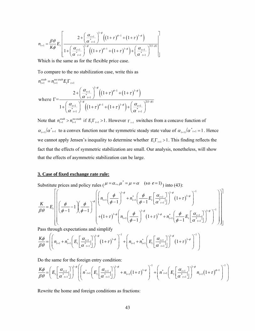
43

11 11

*1

1 1 2(1 )1 11 1

* *1 1

2 1 1

1 1 1

t

tt t

t t

t t

n EK

Which is the same as for the flexible price case. To compare to the no stabilization case, write this as

1 1 1

11 11

*1

1 2(1 )1 11 1

* *1 1

2 1 1where =

1 1 1

stab no stabt t t t

t

t

t t

t t

n n E

Note that 1 1 1 if 1stab no stabt t t tn n E . However

1t switches from a concave function of

*11 tt to a convex function near the symmetric steady state value of *

11 1tt . Hence

we cannot apply Jensen’s inequality to determine whether 1 1t tE . This finding reflects the

fact that the effects of symmetric stabilization are small. Our analysis, nonetheless, will show

that the effects of asymmetric stabilization can be large.

3. Case of fixed exchange rate rule:

Substitute prices and policy rules (*

*, (so 1)e ) into (43):

1111* 1

1 1 *1

1111 1 * 1

1 1 *1

11 1

11 1

1 11 1

tt t t

t

t

tt t t

t

n n EK

E

n n E

Pass through expectations and simplify

1 11 1

1 1* *1 11 1 1 1* *

1 1

1 1t tt t t t t t

t t

Kn n E n n E

Do the same for the foreign entry condition:

1 11 1 1

1 1* *1 1 11 11 1* * *

1 1 1

1 1t t tt tt t t t t

t t t

KE n E n n E n

Rewrite the home and foreign conditions as fractions:

44

Home: * *

1 1 1 1

1 1

t t t t

K

n An n Bn

Foreign: * *

1 11 1t tt t

K A B

n An n Bn

Where we define:

Equating across countries:

Note that the denominator will be negative provided the standard deviation of shocks is small relative to the iceberg costs, which will be true for all our cases:

0.5

1 1 1ln 2/ 1 1 /

2

For shocks independently log normally distributed with standard deviation so that

. For example, with =0.1 and =6, must be less than 0.209. Our calibration of is 0.017.

1*

1

So 1 if 2 2 or 1t

t

nAB A B A B AB

n

For independent log normal distributions of productivity:

We can conclude that n>n*. 4. LCP version of price adjustment costs

Under the specification that prices for domestic sales, tp h , and exports, *tp h , are

set separately in the currencies of the buyers, the Rotemberg price setting equations for our

model become:

1 1

1 11 1* *

1 1

1 , 1t tt t

t t

A E B E

* *11 1 1

* * * *1 11 1 1 1 1 1

2 2 tt t t

t tt t t t t t

n A B n A B n ABn

n An n Bn n An n Bn

1*

1

2

2t

t

n AB A B

n A B

1*

1

2so 1 if 1

2t

t

n AB A B

n A B

211 2

*1

tt

t

E e

1 1 2 1

1 11 1 1* * *

1 1 1

1 1t t tt t t

t t t

AB E E E

2

2 1

11*

1

1 since >1tt

t

E e

45

2 2

1 1 1

2

, 1 1 1

11 ,

11 1

1 2 1

11

t t ttt t

t t t t

H t t ttt

t H t t t

p h p h p hWp h p h

p h p h p h

p h p hE

p h p h

and

2 2* * ** *

* * *1 1 1

2* * *, 1 1 11

1 1* * *1 ,

1 1 11 1 1

1 2 1

1 11

t t t t t tt t t

t t t t t

H t t tt tt t

t H t t t t

W p h p h p hp h p h

e p h p h p h

p h p heE

p h e p h

where , , ,H s M s M sP D and * * *, ,, M s M sH s P D .

46

Table 1. Benchmark Parameter Values Preferences Risk aversion 2 Time preference =0.96

Labor supply elasticity 1/ 1.9 Differentiated goods share 0.38 Non-differentiated goods home bias 0.5 Differentiated goods elasticity = 5.2 Non-differentiated elasticity 15.3 Technology Death rate 0.1 Price stickiness 8.7 Differentiated good trade cost D =0.16

Non-differentiated good trade cost N =0.08 Firm entry adjustment cost 0.25 Shocks:

0.6665 0.6145 0.1328 0.2064

0.3724 0.0447 0.0360 0.0250

0.5194 1.6747 0.1289 0.6588

0.2646 0.4435 0.0474 0.4407

'

5.11 4 1.68 4 9.25 5 3.45 5

1.68 4 1.45 4 1.82 5 6.47 5

9.25 5 1.82 5 6.76 4 7.50 5

3.45 5 6.47 5 7.50 5 1.70 4

t t

e e e e

e e e eE

e e e e

e e e e

47

Table 2a: Unconditional Means under Alternative Policies symmetric

stabilization foreign fixed exchange rate

% difference

n 1.967 1.980 0.63 n* 1.951 1.936 -0.73

H 0.573 0.576 0.61

F 0.569 0.566 -0.56

ym 0.469 0.472 0.68 yd 0.606 0.604 -0.34 ym* 0.466 0.464 -0.58 yd* 0.608 0.612 0.53 c 0.982 0.982 0.00 c* 0.981 0.981 -0.03 p(h) 1.186 1.193 0.60 p*(f) 1.267 1.192 -5.91 w 0.959 0.964 0.60 w* 1.024 0.963 -5.91 p(h)/w 1.239 1.239 0.00 p*(f)/w* 1.238 1.239 0.07 p(h)/pdh 1.239 1.239 0.00 p*(f)/pdf* 1.238 1.239 0.07 rer 1.000 1.000 0.01 TOT-Man 1.001 1.001 0.01 TOT-total 1.000 1.002 0.38 Results come from a stochastic simulation of a second-order approximation to the model.

H represents the share of differentiated goods in overall exports of the home country, and it is computed

* * * *

,1

* * * * * * *, , ,1

( )

( )

t t Kt AC tt

Htt Kt AC t Ht Ht AC H tt t

p h n c h d h d h

p h n c h d h d h P C D

;

Ft represents the counterpart for the foreign country.

48

Table 2b: Standard deviations (percent)

data symmetric

stabilization peg

GDP (U.S.) 2.07 2.62 2.51 GDP*(EU-10) 1.61 1.50 1.83 As ratios to std. dev. of GDP: ne 5.46 4.10 4.34 ne* 3.48 3.65 4.52 c 0.75 0.43 0.45 c* 0.88 0.40 0.34 l 0.87 0.40 0.45 l* 0.96 0.44 0.68

U.S. data are used for home country; an average of the EU-10 for foreign.

49

Table 3: Summary of implications of alternative model specifications for key variables

(1) (2) (3) (4) (5) (6) (7) (8) (9)

bench-mark

no entry

LCP sticky wage

high labor

elasticity

GHH & high

elasticity

labor entry costs

uncor-related shocks

tax shocks

n 0.63 0.00 0.49 2.55 0.68 6.12 0.23 1.27 1.07 n* -0.73 0.00 -0.77 -2.14 -0.76 -7.36 -0.41 -1.45 -1.53 n*-n -1.36 0.00 -1.25 -4.69 -1.44 -13.48 -0.64 -2.73 -2.60

diffshare 0.61 0.05 0.60 1.58 0.64 4.54 0.32 1.22 1.18 diffshare* -0.56 -0.02 -0.54 -1.77 -0.60 -4.78 -0.37 -1.09 -0.88 diffshare*-diffshare -1.17 -0.06 -1.14 -3.35 -1.24 -9.32 -0.69 -2.31 -2.06

Table reports the percent change in a variable when the foreign country replaces inflation stabilization with exchange rate peg. Table also reports the difference between the home and foreign percent changes.

H represents the share of differentiated goods in overall exports of the home country, and it is computed

* * * *

,1

* * * * * * *, , ,1

( )

( )

t t Kt AC tt

Htt Kt AC t Ht Ht AC H tt t

p h n c h d h d h

p h n c h d h d h P C D

;

F represents the counterpart for the foreign country.

50

Table 4: Baseline Regression

(1) (2) (3) (4) (5) (6) (7)

BenchmarkNon-oil

exporting countries

Exclude Low Income

High & Upper Middle Income

High Income & Non-oil

No Energy Goods

Shambaugh Peg

PEG -0.0585*** -0.0635*** -0.0632*** -0.0642*** -0.0234 -0.0487*** -0.0367** (0.0163) (0.0166) (0.0169) (0.0195) (0.0191) (0.0164) (0.0162)

Obs. 3646 3256 2942 2094 953 3645 4757 R-sq 0.741 0.725 0.786 0.816 0.818 0.712 0.718 adj. R-sq 0.728 0.710 0.774 0.805 0.803 0.696 0.706 Country Fixed Effect yes yes yes yes yes yes yes

Year Fixed Effect yes yes yes yes yes yes yes

Notes: DIF not included as regressor because subsumed in fixed effects.

Standard errors (clustered by country) in parentheses:

* significance at 10%; ** significance at 5%; ***significance at 1%

51

Table 5: Baseline Regression with Lagged Peg

(1) (2) (3) (4) (5) (6) (7)

Benchmark Non-oil

exporting countries

Exclude Low Income

High & Upper Middle Income

High Income & Non-oil

No Energy Goods

Shambaugh Peg

PEG -0.0270* -0.0228* -0.0292* -0.0476** 0.0000 -0.0179 -0.0177 (0.0158) (0.0136) (0.0176) (0.0212) (0.0140) (0.0146) (0.0127)

L.PEG -0.0360** -0.0488*** -0.0422*** -0.0188 -0.0253* -0.0345* -0.0257** (0.0154) (0.0157) (0.0156) (0.0145) (0.0130) (0.0181) (0.0124)

Obs. 3481 3113 2809 1997 911 3480 4580

R-sq 0.747 0.731 0.791 0.822 0.820 0.722 0.727 adj. R-sq 0.733 0.715 0.779 0.810 0.805 0.706 0.715 Country Fixed Effect yes yes yes yes Yes yes yes Year Fixed Effect yes yes yes yes Yes yes yes

Notes: DIF not included as regressor because subsumed in fixed effects.

Standard errors (clustered by country) in parentheses:

* significance at 10%; ** significance at 5%; ***significance at 1%

52

Table 6: Baseline Regressions with Controls

(1) (2)

benchmark

5 year averages

PEG -0.0528*** -0.0465**

(0.0186) (0.0221)

CA_GDP 0.000337 0.00101

(0.000619) (0.00181)

RER 0.00855 0.0182*

(0.0122) (0.0101)

CRISIS_C 0.00646 0.0154

(0.0111) (0.0210)

CRISIS_B 0.00521 0.0126

(0.0154) (0.0249)

CLOSED -0.0185 -0.00285

(0.0261) (0.0329)

Obs. 2523 646

R-sq 0.785 0.853

adj. R-sq 0.769 0.804 Country and Year Fixed Effects yes yes

53

Table 7: IV Regressions

IV: Lagged IMF Exchange Rate IV: Klein-Shambaugh Index

PEG -0.0739*** -0.0739*** -0.108*** -0.108***

(0.0206) (0.0104) (0.0273) (0.0133) Obs. 3481 3481 3443 3443 R-sq 0.183 0.183 0.165 0.165 adj. R-sq 0.137 0.137 0.120 0.120 Standard Errors Clustered Robust Clustered Robust Country Fixed Effect yes yes yes yes Year Fixed Effect yes yes yes yes

Notes: DIF not included as regressor because subsumed in fixed effects.

If the instrument is Klein and Shambaugh, the instrumented variable is the Shambaugh peg; If the instrument is the lagged IMF exchange rate index, the instrumented is the contemporaneous IMF exchange rate index.

Under "IV: Klein-Shambaugh Index":

Standard errors (either clustered by country or heteroskedasticity-robust) in parentheses:

* significance at 10%; ** significance at 5%; ***significance at 1%

54

Fig 1. Responses to a 1 std dev rise in home manufacturing productivity;

both countries use efficient stabilization monetary policy

Vertical axis is percent deviation (0.01=1%) from steady state levels. Horizontal axis is time (in years).

5 10 15-0.01

0

0.01

0.02lln

5 10 15-5

0

5

10x 10

-3 lnstar

5 10 15-0.1

0

0.1lym

5 10 15-0.01

0

0.01

0.02lymstar

5 10 15-0.02

-0.01

0

0.01lyd

5 10 150

0.005

0.01

0.015lydstar

home firms

home non-diff. output

home differentiated output

foreign firms

foreign differentiated output

foreign non-diff. output

55

Fig 2. Responses to a 1 std dev rise in home manufacturing productivity;

both countries use efficient stabilization monetary policy; No autocorrelation in shocks across countries

Vertical axis is percent deviation (0.01=1%) from steady state levels. Horizontal axis is time (in years).

5 10 150

0.01

0.02

0.03lln

5 10 15-0.02

-0.01

0

0.01lnstar

5 10 150

0.02

0.04

0.06lym

5 10 15-0.03

-0.02

-0.01

0lymstar

5 10 15-0.02

-0.01

0lyd

5 10 150

0.005

0.01

0.015lydstar

home firms

home non-diff. output

home differentiated output

foreign firms

foreign differentiated output

foreign non-diff. output

56

Fig 3: Responses to a 1 std dev rise in home manufacturing productivity;

foreign country pegs

Vertical axis is percent deviation (0.01=1%) from steady state levels. Horizontal axis is time (in years).

5 10 15-0.01

0

0.01

0.02lln

5 10 15-0.01

0

0.01

0.02lnstar

5 10 15-0.05

0

0.05lym

5 10 15-0.02

0

0.02

0.04lymstar

5 10 15-0.02

-0.01

0

0.01lyd

5 10 15-5

0

5

10x 10

-3 lydstar

home firms

home non-diff. output

home differentiated output

foreign firms

foreign differentiated output

foreign non-diff. output

57

Fig 4. Responses to a 1 std dev rise in foreign manufacturing productivity;

foreign country pegs

Vertical axis is percent deviation (0.01=1%) from steady state levels. Horizontal axis is time (in years).

5 10 15-10

-5

0

5x 10

-3 lln

5 10 150

2

4

6x 10

-3 lnstar

5 10 15-0.02

-0.01

0

0.01lym

5 10 15-5

0

5

10x 10

-3 lymstar

5 10 15-0.02

-0.01

0

0.01lyd

5 10 15-0.01

0

0.01lydstar

home firms

home non-diff. output

home differentiated output

foreign firms

foreign diff. output

foreign non-diff. output