Hindawi Publishing CorporationEURASIP Journal on Image and Video ProcessingVolume 2011, Article ID 458283, 10 pagesdoi:10.1155/2011/458283

Research Article

Camera Network Coverage Improving byParticle SwarmOptimization

Yi-Chun Xu,1 Bangjun Lei,1 and Emile A. Hendriks2

1 Institute of Intelligent Vision and Image Information, China Three Gorges University, 443002, Yichang, China2Department of Mediamatics, Faculty of Electrical Engineering, Mathematics, and Computer Science (EEMCS),Delft University of Technology, 2600 GA Delft, The Netherlands

Correspondence should be addressed to Yi-Chun Xu, yichunx@gmail.com

Received 30 April 2010; Revised 29 July 2010; Accepted 16 November 2010

Academic Editor: Dan Schonfeld

Copyright © 2011 Yi-Chun Xu et al. This is an open access article distributed under the Creative Commons Attribution License,which permits unrestricted use, distribution, and reproduction in any medium, provided the original work is properly cited.

This paper studies how to improve the field of view (FOV) coverage of a camera network. We focus on a special but practicalscenario where the cameras are randomly scattered in a wide area and each camera may adjust its orientation but cannot move inany direction. We propose a particle swarm optimization (PSO) algorithm which can efficiently find an optimal orientation foreach camera. By this optimization the total FOV coverage of the whole camera network is maximized. This new method can alsodeal with additional constraints, such as a variable region of interest (ROI) and possible occlusions in the ROI. The experimentsshowed that the proposed method has a much better performance and a wider application scope. It can be effectively applied inthe design of any practical camera network.

1. Introduction

Video cameras are widely applied to inspect and/or monitorinteresting objects and scenes remotely and automatically[1, 2]. Often, to cover a large area, multiple cameras are con-nected together to form a camera/video network. By actingas an integrated unit, the camera network provides a muchlarger field of view (FOV) coverage than any single camerathat constitutes it. However, the distribution of cameras(locations and orientations) will influence greatly the totalFOV coverage of the camera network. With a fixed numberof cameras, an optimal arrangement—putting cameras at theright locations and orientations—will produce the largestFOV coverage. It subsequently maximizes the effectivenessof the camera network deployment. This optimizationproblem has been studied by, for example, computer visionresearchers from slightly different perspectives, such as 3Dreconstruction [3, 4], target surveillance [5, 6].

The camera network FOV coverage optimization isdefined as the using fewest possible cameras to moni-tor/inspect a fixed area or maximizing the FOV coverageof a network with fixed number of cameras. At present,the video camera is still an expensive sensor (not only in

terms of financial cost but also in terms of bandwidth andcomputation power needed for transmitting and processingits output). That is why the coverage optimization hasattracted a lot of research attention [7]. The oldest coverageoptimizationmay be the Art Gallery Problem (AGP) [8]. Thegoal of AGP is to determine a minimal number of guards andtheir positions, so that all important sites in a polygon areacan be fully under supervision. Because the human guardshave no eyesight limitations (in comparison to the limitedFOV of video cameras), applying AGP directly to cameranetworks is difficult. Erdem and Sclaroff [9] defined a cameraplacement problem similar to AGP, but with a more realisticcamera model. For solving this problem, they proposed a0-1 integer program model for the placement and thenadopted a bound and branch approach. However, it is verydifficult, if not impossible, to globally optimize the formedmathematical model when the problem size becomes large.To avoid this problem, Hsieh et al. [10] limited themselves toseveral special types of scenarios (lanes and circles) and onetype of cameras (omni directional).

Recently, more considerations from real applicationsare taken into account. For instance, unlike the previousmentioned papers trying to minimize the overlapping FOV,

2 EURASIP Journal on Image and Video Processing

Yao et al. [11] suggested that in some applications anoverlapping FOV between the cameras is necessary. One suchexample is the object tracking. The trajectory of an objectshould be maintained across different camera views. For thispurpose a sufficient uniform overlap between neighboringcameras’ FOVs should be secured so that camera handovercan be successful and automated. They proposed sensor-planning methods which add the handoff rate analysis.Zhao and Cheung [12] studied how to arrange the camerasfor tracking visual tags. Their model incorporates realisticcamera models, occupant traffic models, self-occlusion, andmutual occlusion possibilities.

The above-mentioned papers are about the full planfor deploying cameras in a network, where both locationand orientation of each camera can be determined beforeconstructing the network. Recently, Tao et al. [13, 14]studied another type of coverage optimization problem. Intheir system, the cameras were randomly spread over anarea, the location of each camera could not be changed,but the orientation of each camera can be freely adjusted.Their system can be applied for military purposes wherehundreds of cameras with wireless sensors are scatteredby an airplane and quickly form a camera network tomonitor a wide area. For large camera networks this systemis more practical because in most situations the mountinglocations are limited by the physical possibilities. Tao etal. proposed a potential field-based coverage enhancingalgorithm (PFCEA) for solving this problem. In PFCEA,the FOV of each camera is regarded as a virtual particleand can be repelled by other cameras. The virtual force ideafirst appeared in [15], where it was used to deploy omnidirectional sensors. In [13, 14], if the virtual torque on theFOV of a camera is not zero, the camera will adapt its angleaccordingly. They found the coverage of the camera networkwas maximized when the network reached an equilibrium.

In this paper, we base ourselves on the problem modeland application of [13, 14]. Whereas, to overcome thedisadvantage of the PFCEA algorithm (to be explained inSection 4), we propose to use particle swarm optimization(PSO) as the optimization engine. PSO was proposed byKennedy and Eberhart to model birds flocking and fishschooling for food [16]. It is welcomed in practice, becauseit is easy to implement, needs few parameters, and does notrequire the objective function to be differentiable [17]. PSOhas attracted a lot of research attentions in recent years. It hasbeen successfully applied in, for example, training of neuralnetworks [18], control of the reactive power and voltage [19],and cutting and packing problems [20]. We will show thatPSO is also very effective for the camera network coverageproblem. It can achieve global optimization. To prove itssuperior performance, we conduct an extensive comparisonbetween PSO and PFCEA through several experiments. Fur-ther, we will theoretically analyze the optimization feasibilityunder different situations. We therefore find a new effectiveway for optimizing the camera network coverage problemthat is much better than previous approaches. On the otherhand, we explore a new field of applying the PSO algorithm.

Conci and Lizzi [21] also reported on the placementof cameras using PSO. In their method, they assumed

a Rayleigh distribution for characterizing the distance ofthe object and a Gaussian distribution for modeling thehorizontal camera FOV, and, their work mainly focused onan indoor environment where the number of cameras issmall and the PSO performance is not an issue. Our work,on the contrary, is more intended for applications discussedin [13, 14] where hundreds of cameras or more are randomlydistributed in an unknown area. Therefore we focus moreon the performance of the algorithm and the relationshipsbetween the coverage improvement and the scale of thenetwork. This makes our work complementary to [21].

The paper is organized as follows. We first defineour problem model in Section 2. We then introduce ourPSO algorithm in detail in Section 3. Subsequently, weexperimentally show the superior performance of our PSOalgorithm and make comparisons to the PFCEA in Section 4.We then give discussions about the results in Section 5, andfinally, we conclude the paper in Section 6.

2. ProblemModel

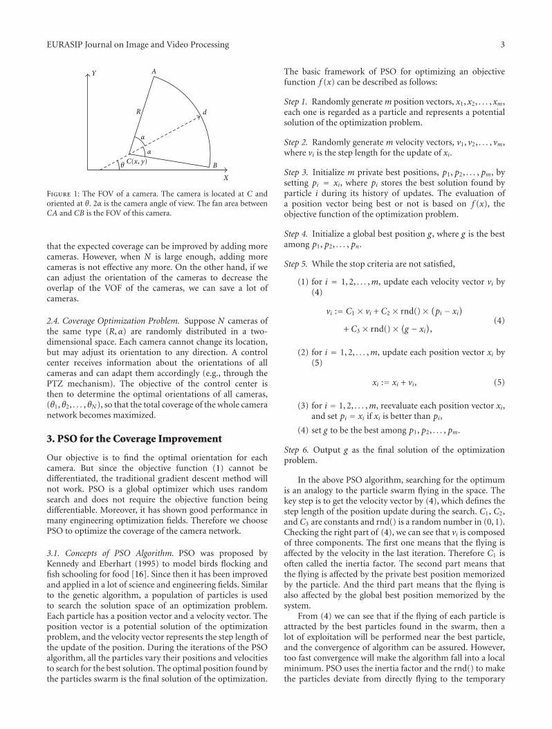
2.1. Camera FOV. The FOV of a camera is defined as afan-shaped area as in Figure 1, where CAB defines the FOVof a camera C. The length of CA or CB is denoted by R,which defines the distance from the camera to the mostdistant objects that appear with an acceptable resolution. Thecamera angle of view is denoted by 2α. The vector d definesthe orientation of the camera and θ is the azimuth. We use(R,α) to note the type of the camera.

2.2. Camera Viewing Coverage. Under aforementioned cam-era FOV model, the viewing coverage c of a camera isdefined as the ratio of the area of the FOV of the camerato the total monitored area S as c = αR2/S. In the cameranetwork, the observed regions of different cameras may beoverlapped with each other.We use an approximate approachto calculate the coverage of a camera network. The totalmonitored area is divided into small regular grids. Thecoverage is then defined as the ratio of the number of coveredgrids to the total numbers of grids:

c = number of covered gridstotal number of grids

. (1)

2.3. Camera Number versus Network Coverage. Suppose Ncameras of the same type (R,α) are distributed randomlyover an area S. The coverage c, defined in the previoussubsection as a probability of the total area being covered, canbe estimated as follows [9]:

c = 1−(1− αR2

S

)N

(2)

or

N = ln(1− c)ln(S− αR2)− ln S

. (3)

Our simulations indeed showed that these equations aresatisfied well for real situations. From (2) we can observe

EURASIP Journal on Image and Video Processing 3

α

α

θ

A

B

X

Y

dR

C(x, y)

Figure 1: The FOV of a camera. The camera is located at C andoriented at θ. 2α is the camera angle of view. The fan area betweenCA and CB is the FOV of this camera.

that the expected coverage can be improved by adding morecameras. However, when N is large enough, adding morecameras is not effective any more. On the other hand, if wecan adjust the orientation of the cameras to decrease theoverlap of the VOF of the cameras, we can save a lot ofcameras.

2.4. Coverage Optimization Problem. Suppose N cameras ofthe same type (R,α) are randomly distributed in a two-dimensional space. Each camera cannot change its location,but may adjust its orientation to any direction. A controlcenter receives information about the orientations of allcameras and can adapt them accordingly (e.g., through thePTZ mechanism). The objective of the control center isthen to determine the optimal orientations of all cameras,(θ1, θ2, . . . , θN ), so that the total coverage of the whole cameranetwork becomes maximized.

3. PSO for the Coverage Improvement

Our objective is to find the optimal orientation for eachcamera. But since the objective function (1) cannot bedifferentiated, the traditional gradient descent method willnot work. PSO is a global optimizer which uses randomsearch and does not require the objective function beingdifferentiable. Moreover, it has shown good performance inmany engineering optimization fields. Therefore we choosePSO to optimize the coverage of the camera network.

3.1. Concepts of PSO Algorithm. PSO was proposed byKennedy and Eberhart (1995) to model birds flocking andfish schooling for food [16]. Since then it has been improvedand applied in a lot of science and engineering fields. Similarto the genetic algorithm, a population of particles is usedto search the solution space of an optimization problem.Each particle has a position vector and a velocity vector. Theposition vector is a potential solution of the optimizationproblem, and the velocity vector represents the step length ofthe update of the position. During the iterations of the PSOalgorithm, all the particles vary their positions and velocitiesto search for the best solution. The optimal position found bythe particles swarm is the final solution of the optimization.

The basic framework of PSO for optimizing an objectivefunction f (x) can be described as follows:

Step 1. Randomly generatem position vectors, x1, x2, . . . , xm,each one is regarded as a particle and represents a potentialsolution of the optimization problem.

Step 2. Randomly generate m velocity vectors, v1, v2, . . . , vm,where vi is the step length for the update of xi.

Step 3. Initialize m private best positions, p1, p2, . . . , pm, bysetting pi = xi, where pi stores the best solution found byparticle i during its history of updates. The evaluation ofa position vector being best or not is based on f (x), theobjective function of the optimization problem.

Step 4. Initialize a global best position g, where g is the bestamong p1, p2, . . . , pn.

Step 5. While the stop criteria are not satisfied,

(1) for i = 1, 2, . . . ,m, update each velocity vector vi by(4)

vi := C1 × vi + C2 × rnd()× (pi − xi)

+ C3 × rnd()× (g − xi),

(4)

(2) for i = 1, 2, . . . ,m, update each position vector xi by(5)

xi := xi + vi, (5)

(3) for i = 1, 2, . . . ,m, reevaluate each position vector xi,and set pi = xi if xi is better than pi,

(4) set g to be the best among p1, p2, . . . , pm.

Step 6. Output g as the final solution of the optimizationproblem.

In the above PSO algorithm, searching for the optimumis an analogy to the particle swarm flying in the space. Thekey step is to get the velocity vector by (4), which defines thestep length of the position update during the search. C1, C2,and C3 are constants and rnd() is a random number in (0, 1).Checking the right part of (4), we can see that vi is composedof three components. The first one means that the flying isaffected by the velocity in the last iteration. Therefore C1 isoften called the inertia factor. The second part means thatthe flying is affected by the private best position memorizedby the particle. And the third part means that the flying isalso affected by the global best position memorized by thesystem.

From (4) we can see that if the flying of each particle isattracted by the best particles found in the swarm, then alot of exploitation will be performed near the best particle,and the convergence of algorithm can be assured. However,too fast convergence will make the algorithm fall into a localminimum. PSO uses the inertia factor and the rnd() to makethe particles deviate from directly flying to the temporary

4 EURASIP Journal on Image and Video Processing

(1) Randomly generatemN-dimensional orientation vectors x1, x2, . . . , xm, andmN-dimensional velocity vectorsv1, v2, . . . , vm. Then evaluate the coverage based on these orientation vectors and get the first private bestposition p1, p2, . . . , pm and the global best g.

(2) While the predefined iterations is not reached(3) for each particle i = 1 tom(4) calculate vi as (4);(5) calculate xi as (5)(6) transform xi in to [0, 2π) and evaluate the coverage based on xi(7) if xi is better than pi, then update pi.(8) if xi is better than g, then update g.(9) end for(10) end while(11) output the global best position g, and the obtained coverage.

Algorithm 1: The PSO algorithm for the coverage optimization.

best particle. Then much more space around can be exploredand the algorithm can jump out from a local minimum. Thisexplains why the PSO generally has a good performance.

3.2. PSO for the Coverage Improvement. The “position vec-tor” defined in the general PSO is a potential solution x whenwe optimize an objective function f (x). The key problemsfor applying PSO are to define the position vector x and theobjective function f (x). To avoid confusion, we use for thecameras the terms “locations” and “orientations” instead ofthe “positions” throughout this paper.

In our coverage improvement problem, we need tooptimize the orientation vector of the cameras, x =(θ1, θ2, . . . , θN ). The objective function is the total coveragedefined in (1). The computation of (1) is based on theorientations, locations, and the type parameters (R,α) ofall cameras. The locations and the type parameters of thecameras are the inputs to the algorithm. The orientations arewhat will be searched for. For all the experiments, we follow[22] to set C1 = 0.729 and C2 = C3 = 1.49445 in (4).

In standard PSO, the velocity v is often bounded in arange of (−V max,Vmax) to avoid a long jump of x that mayresult x(i) missing the optimum. In our experiments, we donot limit the velocity, but transform the orientation of thecamera to a value in the range of [0, 2π). Then the update ofthe x is also bounded.

The algorithm will stop when the number of iterationsis equal to a predefined number, or a predefined coverage isreached. Because the locations of the cameras are randomlygenerated, we cannot predefine the coverage. Therefore inpractice we often use a predefined maximum number ofiterations. The complete algorithm is listed in Algorithm 1.

4. Experiments and Results

Three experiments were carried out to demonstrate theperformance of the PSO for the coverage improvement ofcameras. In Experiment 1, the performance and convergenceof PSO were studied. In Experiment 2, PSO and PFCEAwere compared to each other and the advantages of PSO

0.5

0.55

0.6

0.65

0.7

0 100 200 300 400 500 600 700 800 900 1000

Iteration

Coverage

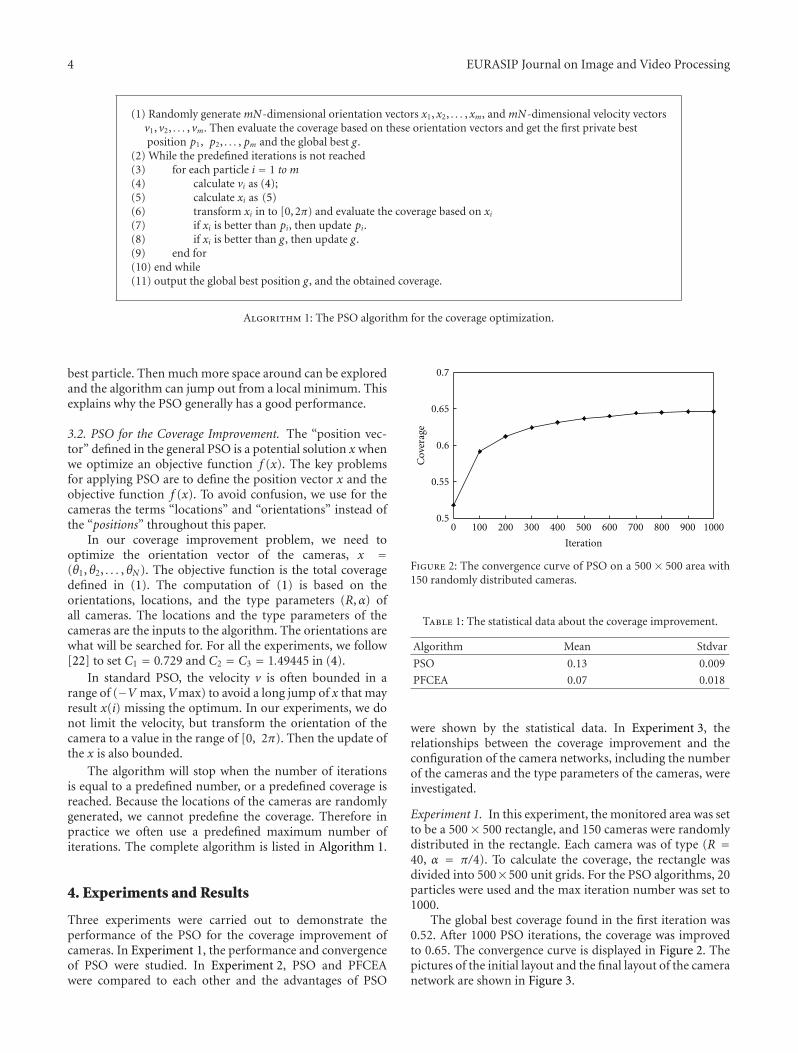
Figure 2: The convergence curve of PSO on a 500 × 500 area with150 randomly distributed cameras.

Table 1: The statistical data about the coverage improvement.

Algorithm Mean Stdvar

PSO 0.13 0.009

PFCEA 0.07 0.018

were shown by the statistical data. In Experiment 3, therelationships between the coverage improvement and theconfiguration of the camera networks, including the numberof the cameras and the type parameters of the cameras, wereinvestigated.

Experiment 1. In this experiment, the monitored area was setto be a 500× 500 rectangle, and 150 cameras were randomlydistributed in the rectangle. Each camera was of type (R =40, α = π/4). To calculate the coverage, the rectangle wasdivided into 500×500 unit grids. For the PSO algorithms, 20particles were used and the max iteration number was set to1000.

The global best coverage found in the first iteration was0.52. After 1000 PSO iterations, the coverage was improvedto 0.65. The convergence curve is displayed in Figure 2. Thepictures of the initial layout and the final layout of the cameranetwork are shown in Figure 3.

EURASIP Journal on Image and Video Processing 5

(a) (b)

Figure 3: The coverage improvement of the PSO. (a) the initial layout. (b) The final improved layout.

As indicated by (2), 150 cameras are expected to reachthe coverage of 0.53. Our initial placement with the coverageof 0.52 was close to this. After the 1000 cycles of PSO,the coverage was raised to 0.65, that is, the coverage wasimproved for about 0.13. If we want to get this coveragewithout optimization, we will need to add another 58randomly placed cameras (total of 208 cameras) as can beseen in Figure 2. In other words, we have saved 58 camerasby improving the coverage using the PSO.

Note that the improvement of the coverage varies withrespect to the random initial configuration of the network,but in Experiment 2 we will show that the coverage improve-ment of the PSO is often stable.

Experiment 2. To show the performance of the PSO further,we ran the program for 30 runs with the same camera num-ber, camera type, and PSO parameters as in Experiment 1.We collected the coverage improvement data, where eachrun started from a random initial configuration. We alsoimplemented PFCEA as described in [9, 10] to make acomparison. In PFCEA, if the virtual torque was greater than10−6, the camera was rotated for π/180, otherwise the camerawas regarded to be in equilibrium. The iteration of PFCEAwas set to 360 in order for each camera to rotate for a fullround (Our experiences also showed that 360 iterations areenough for the convergence of PFCEA, and more iterationsdid not improve the coverage any more.) The collectedstatistical data about the coverage improvement is shownin Table 1. From this we conclude that our PSO statisticallymore significantly improved the coverage than PFCEA andthe performance was more stable.

Actually, because of the limitation of the underlyingprinciple employed, Tao et al.’s PFCEA algorithm cannotachieve the best possible optimization in a camera net-work. As illustrated in Figure 4(a), the two cameras are inequilibrium but the coverage of the two cameras is not aslarge as in Figure 4(b). In view of the optimization, PFCEAtries to use the virtual force as the gradient to search for

A B

(a)

AB

(b)

Figure 4: An illustration of the disadvantage of PFCEA algorithm.(a) Since the two cameras are not allowed translational movement,they are in a balance state. This configuration is considered as theoptimal solution by PFCEA but it is not really optimal becauseof the existence of overlaps. (b) A possible state with maximalcoverage.

the orientations, but because the cameras cannot move, itsoptimization ability is always limited.

Experiment 3. In this experiment, the relationships betweenthe coverage and the three parameters N , R, and α wereinvestigated, and our PSO algorithm was further comparedwith the PFCEA of Tao. In each calculation, the positions ofall the cameras were randomly generated and fed to PSO andPFCEA identically. The settings for PSO and PFCEA were thesame as in Experiments 1 and 2.

The experiment was carried out in three phases withmarginally varying the 3 parameters. Firstly we varied N ,keeping R, and α fixed. Then we varied R, keeping N , andα fixed. Finally we varied α, keeping instead N and R fixed.The parameters of the camera networks are shown in Table 2,the results are illustrated in Figure 5.

The main results that we can conclude from Figure 5 arethe following.

(a) PSO performed better than PFCEA in all threephases. In mostcases, the coverage improvement of

6 EURASIP Journal on Image and Video Processing

Table 2: The parameters of the camera networks in Experiment 2.

S N R α

Phase 1 500× 500 rectangle Varied from 50 to 600 40 π/4

Phase 2 500× 500 rectangle 100 Varied from 20 to 100 π/4

Phase 3 500× 500 rectangle 100 40 Varied from π/6 to 3/4π

0

0.2

0.4

0.6

0.8

1

50 100 200 300 400 500 600

Number of cameras

Coverage

Expected coverageCoverage by PSOCoverage by PFCEA

(a)

0

0.2

0.4

0.6

0.8

1

Coverage

Expected coverageCoverage by PSOCoverage by PFCEA

20 40 60 80 100

R of FOV

(b)

0

0.2

0.4

0.6

0.8

1

Coverage

Expected coverageCoverage by PSOCoverage by PFCEA

2/12π 3/12π 4/12π 5/12π 6/12π 7/12π 8/12π 9/12π

α of FOV

(c)

0

0.05

0.1

0.15

0.2

0 0.2 0.4 0.6 0.8 1

Expected coverage

Coverageim

provem

ent

Number of cameras

α of FOVR of FOV

(d)

Figure 5: The relationships between the parameters and the coverage. (a) Relationship of (c,N); (b) relationship of (c,R); (c) relationshipof (c,α); (d) relationship of the coverage increment by PSO and the initial coverage.

PSO was nearly twice as large as that of PFCEA.We believe that this is because PSO is a globaloptimization technique and the global coverage isthe objective of this optimization. In contrast, theobjective of PFCEA is balancing the virtual torqueand the optimization of coverage is indirect. There-fore no global optimal coverage can be obtained.That is why in some rare cases PFCEA even decreasesthe coverage, as can be seen in Figure 5(c) (cameraangle of view equal to 2/12 π, the initial coverageequal to 0.279, and after the processing of PFCEA, thecoverage became 0.267).

(b) when the initial coverage was very small or very large,the improvement was small. This finding was firstclaimed in [9], and consistent with the experimentsin this paper, as shown in Figure 5(a), 5(b), and5(c). The reason to this is that if the initial coverage

is very small, the overlap between the FOV of thecameras will also be small in general, and then theimprovement cannot be very large. A contradictorycase is that the small initial coverage is caused bythe heavy overlap of FOV, but because the initialdeployment is random, the coverage should obey (2),then this special case rarely appears. On the otherhand, when the initial coverage is very large, thereis little space left for improvement, and then it isimpossible for any algorithm to find large uncoveredspaces.

(c) to get a clearer picture about the relationship betweenthe initial coverage and the coverage improvement,we used the initial coverage as x-axis and the coverageimprovement as y-axis, and we got three curves asin Figure 5(d), which are derived from Figures 5(a),5(b), and 5(c). We can observe again that, when

EURASIP Journal on Image and Video Processing 7

0

0.2

0.4

0.6

0.8

1

1.2

50 100 150 200 250 300 350 400 450 500 550 600

Number of camera

Exp

ectedcoverage

Expected coverageUpbound of coverage

(a)

00.050.10.150.20.250.30.350.4

0 0.1 0.2 0.3 0.4 0.5 0.6 0.7 0.8 0.9 1

Expected coverage

Coverageim

provem

ent

(b)

Figure 6: Relationship of the coverage improvement and the expected coverage. (a) Curves of expected coverage, upper bound of coverage;(b) relationship of the expected coverage and the coverage improvement.

the initial coverage was too small or too large, theimprovement was small. When the initial coveragewas near 0.6, the PSO obtained the greatest coverageimprovement.

5. Discussions

5.1. The Expected Coverage for the Probably Maximal Cover-age Improvement. The experiments in the previous sectiondemonstrated that the PSO can improve the coverage themost when the initial coverage is about 0.6 but has less effectwhen it is close to 0 or 1. Considering that we can get theexpectation (expected coverage) of this initial coverage by(2), we will explain the results theoretically. That is, we wantto show that when the expected coverage is near 0.6, therewill be maximum space for the improvement.

Assuming that there is no overlap between any twocameras in a camera network, we have a maximum coveredarea. Therefore, we can define the upper bound of thecoverage (cub) of N cameras in type of (R,α) as follows.

cub = min

(NαR2

S, 1

). (6)

With (2) and (6), we then have an upper bound of thecoverage improvement

delta−cub = min

(NαR2

S, 1

)−⎛⎝1−

(1− αR2

S

)N⎞⎠. (7)

Let us consider the relationship of delta−cub and N with(R,α) and S being constant. From (7) we can conclude thatdelta−cub is a monotonically increasing function of N whenNαR2/S ≤, and a monotonically decreasing function whenNαR2/S ≥ 1. Then we get the maximum improvement whenNαR2/S = 1.

Replacing αR2/S with 1/N in the expected coverage (2),

c = 1−(1− αR2

S

)N

= 1−(1− 1

N

)N. (8)

We know that when N is large enough (e.g., above 100 inthis paper), (1−(1/N))N → e−1 yielding c = 1−e−1 = 0.635.This means that when the expected coverage near 0.6, wecould get the maximum coverage improvement. This valueis close to our observations from the experiments.

In Figure 6(a) we plot the expected coverage c and theupper bound of the coverage cub as the function of N , whereS is set to 500 × 500, cameras are of type (R = 40, α =π/4). From this figure we derive Figure 6(b) in which weplot the coverage improvement delta−cub as a function of theexpected coverage c. In Figure 6(b), we can clearly see thatthe upper bound of coverage improvement is small when theexpected coverage is near 0 or 1, and is maximal when theexpected coverage is near 0.6.

5.2. Adaptive ROI with the Proposed PSO. PFCEA adjuststhe orientations of the cameras to enlarge the FOV of thecamera network. However, the larger FOV does not alwaysmean higher coverage. Some applications need the cameranetwork to cover a special region of interest (ROI). As PFCEAcannot relate the ROI with the FOV of the camera network,new approaches must be developed. In our proposed PSO,ROI and FOV are related by (1), so our method can workwell without any modification.

Always, constraints should be considered in real appli-cations, such as ROI differences, and the occlusions byobstacles. We still assume that the cameras are alreadyinstalled, and we are required to adjust orientations of thecameras to improve the coverage of the network. Given thatareas that are not in the ROI need not be covered, thedefinition of coverage is changed into

c = number of covered grids in ROItotal number of grids

. (9)

(a) Different ROI at Different Time. In some applications,the ROI of the system varies depending on the surveillanceobjective. For example in Figure 7, two cameras installed onthe wall should monitor A1 (working area) in the daytime,

8 EURASIP Journal on Image and Video Processing

C1

C2

A1

A2

A3

(a)

C1

C2

A1

A2

A3

(b)

Figure 7: The results of PSO for different ROIs. (a) Two cameras C1 and C2 are arranged to monitor A1 in the daytime. (b) They monitorA2 and A3 in the night.

C1

C2

A

B

(a)

C1

C2

A

W

B

(b)

Figure 8: The results of PSOwhen ROI is occluded. (a) CameraC1 monitorsA and camera C2 monitors B. (b)When the obstacleW appears,PSO finds new orientations for the two cameras.

monitorA2 andA3 (two doors) in the night. The size of roomis 100×100. The area A1 is a rectangle of 30×60 and locatednear the center of the western wall. The area A2 and A3 arerectangles of 10 × 20 and located at the two corners besidethe eastern wall. Two cameras C1 and C2 are of type (R = 60,α = π/2) and installed at the center of northern and southernwall of the room.

Then we can use PSO to compute the optimal orientationof the two cameras in the two periods. The results are listedin Table 3, and shown in Figures 8(a) and 8(b) illustrating thesolution in the daytime and the night. Note that because theROI in the daytime and in the night is different, we cannotcompare the coverage in the two cases.

(b) ROI Is Occluded by Obstacle(s). In this example shown inFigure 8, a room of 100 × 100 is monitored by two camerasC1 and C2, where C1 located at the northwest corner and C2

located at the southeast corner and both cameras are of type

Table 3: The orientations of the cameras by PSO for different ROI.

Orientation ofC1 (radians)

Orientation ofC2 (radians)

Coverage

Day time 2.330290163 3.732819163 0.2234

Night 0.128384856 5.845456163 0.0410

(R = 100, α = π/4). The ROI is the area occupied by tworectangles A and B with the same size of 50× 50.

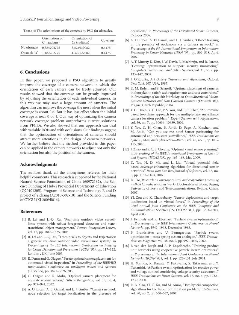
At first, we get a solution by PSO as in Figure 8(a), wherecamera C1 is arranged to monitor area A and camera C2 isarranged to monitor B. Figure 8(b) shows the solution whenan obstacle W appears in the room and the initial FOV ofC1 is occluded. As a result, the PSO provides a new solution,letting C1 monitor B and C2 monitor A. The results are listedin Table 4. We note that the coverage is maintained after theadjustment of the orientations of the two cameras.

EURASIP Journal on Image and Video Processing 9

Table 4: The orientations of the cameras by PSO for obstacles.

Orientation ofC1 (radians)

Orientation ofC2 (radians)

Coverage

No obstacle 0.384704775 3.524939082 0.4475

ObstacleW 1.182262775 4.322527082 0.4475

6. Conclusions

In this paper, we proposed a PSO algorithm to greatlyimprove the coverage of a camera network in which theorientation of each camera can be freely adjusted. Ourresults showed that the coverage can be greatly improvedby adjusting the orientation of each individual camera. Inthis way we may save a large amount of cameras. Thealgorithm can improve the coverage themost when the initialcoverage is about 0.6. But it has less effect when the initialcoverage is near 0 or 1. Our way of optimizing the cameranetwork coverage problem outperforms current solutionsfrom PFCEA. We also showed that our approach can dealwith variable ROIs and with occlusions. Our findings suggestthat the optimization of orientations of cameras shouldattract more attentions in the design of camera networks.We further believe that the method provided in this papercan be applied in the camera networks to adjust not only theorientation but also the position of the camera.

Acknowledgments

The authors thank all the anonymous referees for theirhelpful comments. This research is supported by theNationalNatural Science Foundation of China (60972162), the Sci-ence Funding of Hubei Provincial Department of Education(Q20101205), Program of Science and Technology R and Dproject of Yichang (A2010-302-10), and the Science Fundingof CTGU (KJ 2009B014).

References

[1] B. Lei and L.-Q. Xu, “Real-time outdoor video surveil-lance system with robust foreground detection and state-transitional object management,” Pattern Recognition Letters,vol. 15, pp. 1816–1825, 2006.

[2] B. Lei and L.-Q. Xu, “From pixels to objects and trajectories:a generic real-time outdoor video surveillance system,” inProceedings of the IEE International Symposium on Imagingfor Crime Detection and Prevention ( ICDP ’05), pp. 117–122,London , UK, June 2005.

[3] E. Dunn andG. Olague, “Pareto optimal camera placement forautomated visual inspection,” in Proceedings of the IEEE/RSJInternational Conference on Intelligent Robots and Systems(IROS ’05), pp. 3821–3826, 205.

[4] G. Olague and R. Mohr, “Optimal camera placement foraccurate reconstruction,” Pattern Recognition, vol. 35, no. 4,pp. 927–944, 2002.

[5] A. O. Ercan, A. E. Gamal, and L. J. Guibas, “Camera networknode selection for target localization in the presence of

occlusions,” in Proceedings of the Distributed Smart Cameras,October 2006.

[6] A. O. Ercan, A. El Gamal, and L. J. Guibas, “Object trackingin the presence of occlusions via a camera network,” inProceedings of the 6th International Symposium on InformationProcessing in Sensor Networks (IPSN ’07), pp. 509–518, April2007.

[7] A. T. Murray, K. Kim, J. W. Davis, R. Machiraju, and R. Parent,“Coverage optimization to support security monitoring,”Computers, Environment and Urban Systems, vol. 31, no. 2, pp.133–147, 2007.

[8] J. O’Rourke, Art Gallery Theorems and Algorithms, Oxford,New York, NY, USA, 1987.

[9] U. M. Erdem and S. Sclaroff, “Optimal placement of camerasin floorplan to satisfy task requirements and cost constraints,”in Proceedings of the 5th Workshop on Omnidirectional Vision,Camera Networks and Non Classical Cameras (Omnivis ’04),Prague, Czech Republic, 2004.

[10] Y. C. Hsieh, Y. C. Lee, P. S. You, and T. C. Chen, “An immunebased two-phase approach for the multiple-type surveillancecamera location problem,” Expert Systems with Applications,vol. 36, no. 7, pp. 10634–10639, 2009.

[11] Y. Yao, C. H. Chen, B. Abidi, D. Page, A. Koschan, andM. Abidi, “Can you see me now? Sensor positioning forautomated and persistent surveillance,” IEEE Transactions onSystems, Man, and Cybernetics—Part B, vol. 40, no. 1, pp. 101–115, 2010.

[12] J. Zhao and S. C. S. Cheung, “Optimal visual sensor planning,”in Proceedings of the IEEE International Symposium on Circuitsand Systems (ISCAS ’09), pp. 165–168, May 2009.

[13] D. Tao, H. D. Ma, and L. Liu, “Virtual potential fieldbased coverage-enhancing algorithm for directional sensornetworks,” Ruan Jian Xue Bao/Journal of Software, vol. 18, no.5, pp. 1152–1163, 2007.

[14] D. Tao, Research on coverage control and cooperative processingmethod for vedio sensor networks, Doctoral dissertation, BeijingUniversity of Posts and Telecommunications, Beijing, China,2007.

[15] YI. Zou and K. Chakrabarty, “Sensor deployment and targetlocalization based on virtual forces,” in Proceedings of the22nd Annual Joint Conference on the IEEE Computer andCommunications Societies (INFOCOM ’03), pp. 1293–1303,April 2003.

[16] J. Kennedy and R. Eberhart, “Particle swarm optimization,”in Proceedings of the IEEE International Conference on NeuralNetworks, pp. 1942–1948, December 1995.

[17] B. Brandstatter and U. Baumgartner, “Particle swarmoptimization—mass-spring system analogon,” IEEE Transac-tions on Magnetics, vol. 38, no. 2, pp. 997–1000, 2002.

[18] F. van den Bergh and A. P. Engelbrecht, “Training productunit networks using cooperative particle swarm optimisers,”in Proceedings of the International Joint Conference on NeuralNetworks (IJCNN ’01), vol. 1, pp. 126–131, July 2001.

[19] H. Yoshida, K. Kawata, Y. Fukuyama, S. Takayama, and Y.Nakanishi, “A Particle swarm optimization for reactive powerand voltage control considering voltage security assessment,”IEEE Transactions on Power Systems, vol. 15, no. 4, pp. 1232–1239, 2000.

[20] R. B. Xiao, YI. C. Xu, and M. Amos, “Two hybrid compactionalgorithms for the layout optimization problem,” BioSystems,vol. 90, no. 2, pp. 560–567, 2007.

10 EURASIP Journal on Image and Video Processing

[21] N. Conci and L. Lizzi, “Camera placement using particleswarm optimization in visual surveillance applications,” inProceedings of the IEEE International Conference on ImageProcessing (ICIP ’09), pp. 3485–3499, November 2009.

[22] M. Clerc and J. Kennedy, “The particle system—exploration,stabilty, and convergence in a multidimensional complexspace,” IEEE Transactions on Evolutionary Computation, vol. 6,no. 1, pp. 53–58, 2002.