Embed Size (px)
Citation preview
Caste versus Class: Social Mobility in India 1870-2010 compared to England, 1086-2010
Gregory Clark, University of California, Davis
Zach Landes1
This paper compares rates of social mobility in modern England 1858-2010, in medieval England 1300-1600, and India 1870-2010. Both medieval and modern England are societies of complete long run social mobility. There are no persistent classes. But mobility rates are always low, and are little higher in modern England than in the middle ages. Bengal 1942-2010 shows signs of very little social mobility, with an entrenched and persistent elite that cannot be found even in medieval England. In colonial Bengal 1870-1942 there was clearly mobility, and at rates as high as those of England 1858-1947.
Methods
The question posed here is simple conceptually. If we take a snapshot of a society at a moment
in time we will find a distribution of people by social status, which typically follows a log normal
distribution if we look at quantifiable aspects such as income or wealth, as is portrayed in figure 1.
Suppose we took the people who constitute the top x%, or the bottom x%, of this distribution. Will
their descendants eventually be distributed in terms of wealth or status just like the general
population? If not we have a society permanently divided by class or caste. And if there will be
eventual equality, how long will it take for this equalization of their status with that of the general
population to be accomplished?
To answer this question we use here the only marker of their earlier social status that most
people in society carry, which is their surname. In many social arrangements, including England and
parts of India, surnames are passed unchanged between fathers and sons. In a society of complete
long run social mobility all common surnames will eventually have the same average social status.
However, in societies such as England when surnames were being formed in the years 1066-1350
the type of surname a person held was closely linked to their economic status at the time of
formation. Thus ten percent of English surnames derive from the occupation of the original bearer.
And there is another class of surnames that was largely the preserve of the upper classes, those that
denote a place such as Packenham, and Baskerville. This as we shall see, allows us to easily track
social mobility in England 1086-1500.
1 With thanks to Lincoln Atkinson for his great help in digitizing the 2.2 million names of the Kolkata voters roll of 2010.

Figure 1: The Distribution of Wealth in General and among the Elite.
After 1600 common surnames in England had the same economic and social status. But in
England a significant fraction of the population holds rare surnames. We have measures of what
surnames were rare in England after 1540 from a variety of sources: from 1538-1840 Boyd’s
marriage index which lists 7 million surnames of people married in England, and the national
censuses of 1841-1911. Figure 2, for example, shows the share of the population holding surnames
held by 50 people or less, for each frequency grouping, in the 1881 census. The vagaries of spelling
and transcribing handwriting mean that, particularly for many of the surnames in the 1-5 frequency
range, this is just a recording or transcription error. But for names in the frequency ranges 6-50
most will be genuine rare surnames. Thus in 1881 5 percent of the population, 1.3 million people,
held 92,000 rare surnames. Such surnames arose in various ways: immigration of foreigners, name
mutations from common surnames, or just names that were always rare.
Through two forces – the fact that many of those with rare names were related, and the
operation of chance – the average wealth levels of those with rare surnames will vary greatly at any
time. We can thus divide people post 1600 into constructed social and economic strata by focusing
on those with rare surnames.
0.0
0.2
0.4
0.6
0.8
1.0
1 10 100
Wealth
All
Elite

Figure 2: Relative Frequency of Rare Surnames, 1881 Census, England
We can follow the economic and social success of those with rare surnames all the way from
1600 to 2010 using a variety of sources. The first are probate records which after 1858 give an
indication of the wealth at death of everyone by surname.2 The second is the death register which
allows me to calculate the age at death of most people with rare surnames dying in England 1841-66,
and of all people 1867-2005.3 Average age at death in all periods is a good index of socio-economic
status. The third are public records of address and occupation, such as the electoral register, which
become available for later years.
In India also surnames originally were linked with social status. In the area we focus on,
Bengal, there are a set of surnames, for example, that were exclusively associated with the highest
status groups within the Hindu Brahmin caste: Mukhopadhyaya (Mukherjee), Bandopadhyaya
(Banerjee), Chattopadhyaya (Chatterjee), Bhattacharya (Bhattacharjee), Gangopadhyaya (Ganguli),
Goswami (Gosain). These names belonged to the so-called Kulin Brahmins, who supposedly
migrated to Bengal from north India in the 10th or 11th centuries AD. If they maintained this status
by descent into the modern era then this implies a society of astonishing social rigidity. However,
here we will just look at social mobility using these names for 1870-2010.
2 Those not probated typically have wealth at death close to 0. 3 For people dying 1841-1866 with rare names we can infer age at death for most of them from the censuses and the birth register.
0.0
0.5
1.0
1.5
2.0
2.5
1-5 6-10 11-20 21-30 31-40 41-50
Perc
ent o
f al
l nam
es
There were other names less caste specific that similarly denoted high status: Thakur or Tagores
(landlord), Chakraborty (Chakravarti), Majumdar [friend of the emperor], Ray/Roy, Choudhary, Roy
Chowdhury, Mishra. These surnames were already in use in Bengal by the mid eighteenth century,
as evidenced by the names of zamindars appointed by the East India Company in the eighteenth
century.
To measure the rate of social mobility we need just measure how long it takes the descendants
of an elite, as portrayed in figure 1, to have a wealth or status distribution indistinguishable from the
general population. Or equivalently we can measure how long it takes for a lower class to have
descendants who are distributed like the general population.
The speed of convergence of any elite or subordinate group to the general distribution is
dependent on two things: b, which measures the extent of regression to the mean over a single
generation, and σ2u the variance of the error in the generation of status. Thus if we measure the
logarithm of the income or wealth of the parents relative to the mean by y0, and that of the children
by y1 then we can estimate empirically the value of the coefficient b through the expression
y1 = by0 + u0 (1)
As long as the distribution of income/wealth is stable over time then b and σ2u will be related. Thus
in the long run
1
To get a given wealth distribution, a society with more regression to the mean has to have more
observed “error” in the generation of wealth. The higher is b the more predictable a person’s wealth
or status will be.
In a society with complete eventual regression to the mean, how many generations will it take
for the top x% of the wealth distribution to have descendants equally distributed across the social
spectrum? We can measure how elite a group is by looking at its relative representation at different
points in the wealth distribution. This is just defined as
Below we assume a group has fully regressed to the mean when their relative representation is within
0.9-1.1 for both the top and bottom 5% of the population.

To answer this question we employ a simulation where we assume that wealth overall is distributed
log normally with a variance of 3.24. Assume also that b = .5, a value similar to that estimated for
recent years in the USA and UK.4
To make the simulation easier we assume an elite group whose median wealth is at the 95
percentile of the distribution, and whose wealth is also log normally distributed with the same
variance as the population. With this stipulation 50% of the elite have wealth in the top 5% of the
wealth distribution, and 0% have less wealth than the bottom 5%. What happens to this elite over
succeeding generations? As figure 3 shows, even though in the first generation the relative
representation of the elite in the top 5% is 10 times their share of the population, this ratio falls
rapidly, with (RR-1) essentially halving in each generation. In five generations the relative
representation in the top 5% is only 1.11, whilst the relative representation in the bottom group is
0.91, close to the 10% bound we suggested above.
With this setup the decline in relative representation is most dramatic in the first generation,
and becomes much more gradual later. Here the progress of the RR at the top 5% is 10, 4.1, 2.2,
1.5, 1.23, 1.11. What we will do below is look at the relative representation of elite groups in the top
1-10% of societies over time, and infer from that what the implied b is for that society and time
period.
Another advantage of looking at mobility over multiple generations is that it avoids having to
assume that the mobility process is Markov in nature – that is that the only thing that matters in
each generation is the status of the parents in the previous generation.
4 In practice modern estimates of b vary between 0.2 and 0.6, implying substantial regression to the mean (Solon, 1999). With a stable distribution of wealth or income over time, b also indicates how much of the variation in income in societies is explicable from inheritance. The share so explained will be b2. This means that with a b of 0.5, only about 0.25 of the variance of incomes in each generation is explained by inheritance.

Figure 3: Relative Representation of an Elite over time
Social Mobility in England, 1086-1752
Surnames attached themselves first to the upper classes, and then to the lower classes in
medieval England. Thus already in the Domesday book of 1086 a significant fraction of the major
land owners are identified by surnames, mostly surnames derived from the village they originated
from in France. The process of formation of hereditary surnames was largely complete by 1350.
We can see this in the 1381 poll tax lists when many workers had occupational surnames that
differed from their listed occupation.
To measure social mobility in England 1086-1600 we look at three groups of people. The first
are those with surnames derived from low status occupations: names such as Smith, Mason, Baker,
Shepherd. Since the great majority of the population had hereditary surnames by 1381, we can track
mobility with these names for the period 1300 on by looking at the share of the elite with such
names. The measure we have for the elite 1180-1752 are the surnames of men associated with
Oxford or Cambridge universities. These universities were the great seats of learning in pre-
industrial England. For these years we currently have 14,768 surnames of men who attended
Oxford pre 1500, and 76,047 surnames of men who attended Cambridge in the years before 1752.5
5 There are further lists of names for Oxford 1500-40, and Cambridge before 1500, and Cambridge 1753-1909 that we are in the process of compiling.
0
2
4
6
8
10
12
0 30 60 90 120 150 180 210
Rel
ativ
e R
epre
sent
atio
n
Years
Top 5%
Bottom 5%

How elite a share of the English population attended Oxford or Cambridge in these years? The
number of men born per year in England 1480-99, and surviving to age 15, would be about 20,600.6
179 men per year are recorded first at Oxford and Cambridge in 1480-99 (this number depends on
record survival, so will be a lower bound). Thus entrants to the university represented 0.9% of the
male cohort in these years. Entry to the university was a prelude in these years to service at the
university, in the church, in law, or in government. The students of Oxford and Cambridge thus
constituted an elite of between the top 2 and 5% of the population (not all the social elite attended
the universities).
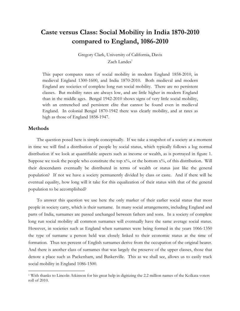
The first measure we have is the percentage of the population with artisan or lower surnames
attending Oxford or Cambridge by 20 year periods, 1180-1752. Figure 4 shows this share. As can
be seen the share of the members of the university drawn from occupational surnames of artisan or
lower status increase dramatically between 1260 and 1500, from 0 percent to around 8 percent, the
share of such names in the later population. Thereafter the share stabilizes. Those of artisan origins
have been fully incorporated into this educational elite. The entire process takes roughly 6-7
generations (180-210 years). So despite being very complete it is not particularly fast.
Since we have evidence that entry to Oxford and Cambridge represented the top 1-2% of the
society, we can actually estimate the rate of regression to the mean. We assume that the artisans
initially were concentrated at the median of socio-economic position in the society. They outranked
the large population of landless agricultural laborers, and of domestic servants. For a given
dispersion of wealth and income their dispersion to the upper 2% of the society can be predicted
from just (1-b), the rate of regression to the mean, since this also determines the extent of the
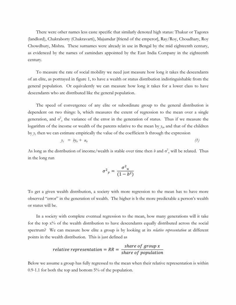
random shocks to social position in each generation. Figure 5 shows the actual rate of occurrence
of artisan surnames relative to the share in the population at Oxbridge, where 0 is 1300 (since only
then have many artisan surnames been created). They completely converge on their population
share by 1500, 6-7 generations. Also shown is the simulated path of convergence for b = 0.5 and b
= 0.8, on the assumption that Oxbridge represented the top 2% of the distribution.
It is clear that b, the measure of persistence, must be significantly greater than 0.5. The closest
fit, assuming Oxbridge the top 2% of the socio-economic distribution, comes from a b of 0.75.
Figure 6 shows how well the different estimates of persistence fit if we instead assume Oxbridge
entrants represented the top 1% of the population. This would imply a b of 0.7. Similarly if
Oxbridge represented only the top 5% of the population the b would be even higher, between .75
and 0.8.
6 Assuming a total population of 2.4 million, a crude birth rate of 35, and that 60% of males survived to age 15.
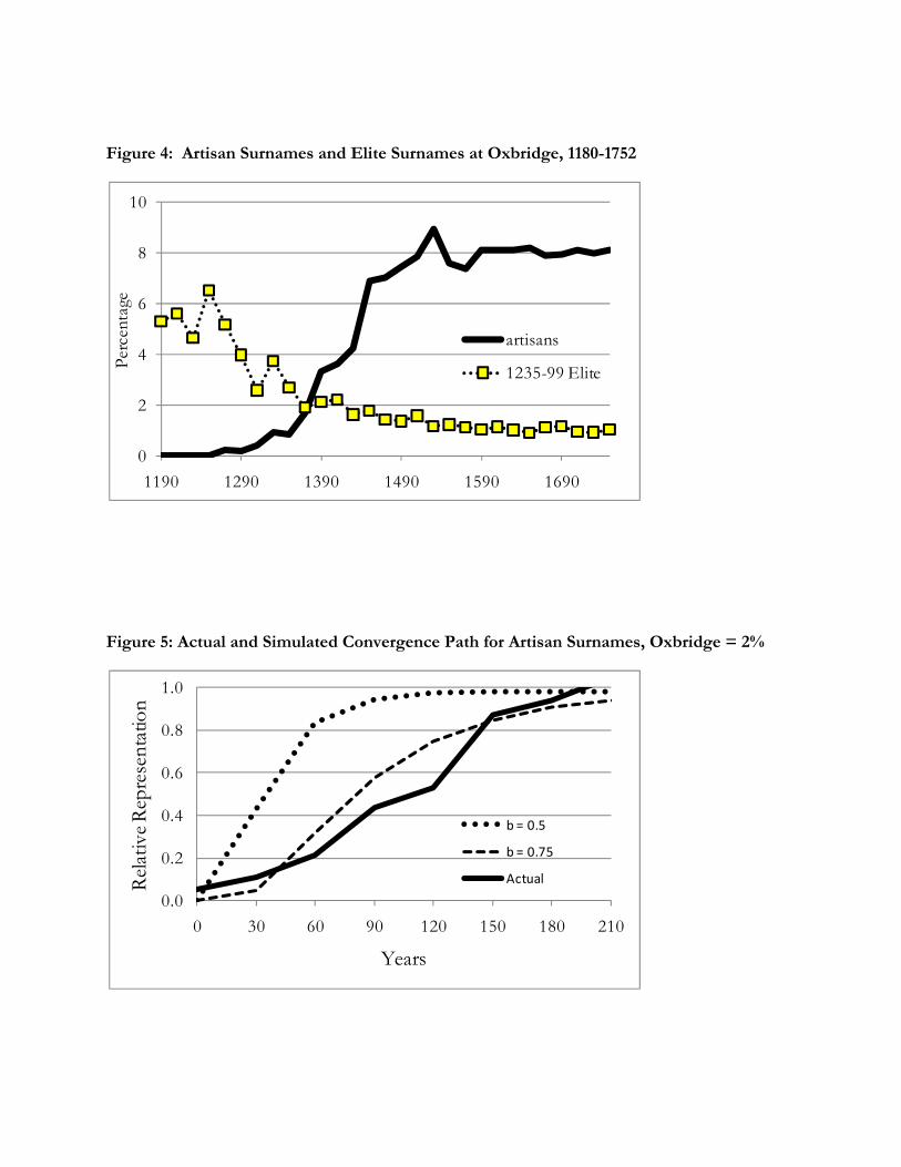
Figure 4: Artisan Surnames and Elite Surnames at Oxbridge, 1180-1752
Figure 5: Actual and Simulated Convergence Path for Artisan Surnames, Oxbridge = 2%
0
2
4
6
8
10
1190 1290 1390 1490 1590 1690
Perc
enta
ge
artisans
1235-99 Elite
0.0
0.2
0.4
0.6
0.8
1.0
0 30 60 90 120 150 180 210
Rel
ativ
e R
epre
sent
atio
n
Years
b = 0.5
b = 0.75
Actual

Figure 6: Actual and Simulated Convergence Path for Artisan Surnames, Oxbridge 1%
These estimates of b show that while mobility was complete on this measure in pre-industrial
England, it was also at rates per generation that would be regarded as extremely low by modern
researchers. However, we shall see that modern estimates for England 1858-2011 do not suggest
much higher rates.
The next thing we can look at is the movement in the share of earlier elites attending Oxford
and Cambridge over time. We have two groups of elite surnames. The first are the surnames of
Normans and Bretons holding estates in England recorded in 1086 in the Domesday Book. Such
names were mainly derived from the home places of these men in France, and are quite distinctive in
England: Baskerville, Darcy, Percy, Coleville, Maundeville, Montgomery. The second are surnames
of a sample of men holding estates as tenants in chief of the King in 1235-99, as revealed in the
Inquisitions Post Mortem. This included many descendants of the Norman and Breton conquerors
of 1066, but also new families that had arisen since then. Figure 7 shows the relative representation
of these names among Oxbridge members by 20 year period 1180-1752 - that is the share of these
surnames in Oxbridge relative to the share in the general population. The share in the general
population is estimated from Boyd’s Marriage Index, a catalogue of the names of grooms and brides
in marriages 1538-1599. This number will be 1 for a group distributed across the socio-economic
ladder in the same way as the general population.
0.0
0.2
0.4
0.6
0.8
1.0
0 30 60 90 120 150 180 210
Rel
ativ
e R
epre
sent
atio
n
Years
b = 0.7
b = 0.8
Actual
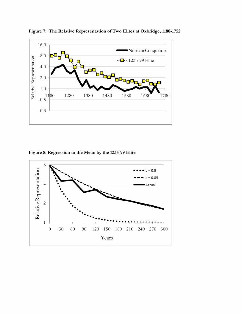
Figure 7: The Relative Representation of Two Elites at Oxbridge, 1180-1752
Figure 8: Regression to the Mean by the 1235-99 Elite
0.3
0.5
1.0
2.0
4.0
8.0
16.0
1180 1280 1380 1480 1580 1680 1780
Rel
ativ
e R
epre
sent
atio
n
Norman Conquerors
1235-99 Elite
1
2
4
8
0 30 60 90 120 150 180 210 240 270 300
Rel
ativ
e R
epre
sent
atio
n
Years
b = 0.5
b = 0.85
Actual

The Norman elite are overrepresented at Oxbridge, 1180-1380, but their overrepresentation
declines steadily from 1260 on. After 1380 they are indistinguishable from the general population.
If this is symptomatic of their general position in society we can say that in 10 generations the
conquerors of 1066 have been completely absorbed into the middle and lower ranges of English
society. This is again complete mobility, but not rapid mobility, as we shall see below.
The other elite is a sample of the upper class from 1235-99. This, as noted, overlaps with the
earlier Norman elite, but is by 1200-1299 much more heavily overrepresented at Oxbridge, as can be
seen in figure 7. For this group the members have a relative representation of 8 in these years at
Oxbridge, compared to 3 for the earlier Norman elite. Their relative representation declines steadily
over the next 480 years, but is still not at 1 by 1752. Indeed in the early eighteenth century those
carrying the same surnames as this earlier elite were still 38% more likely to be at Oxbridge than a
general member of the population.
To estimate the mobility rate of this 1235-99 elite turn to figure 8. This shows the relative
representation of this elite at Oxbridge over 10 generations, where generation 0 is 1270-1299. Also
shown is the implied representation, given the starting point in generation 0, for a b of 0.5 and 0.85,
and the assumption that Oxbridge was the top 2% of the population. The assumption here is that
the elite had the same variance of status as the general population, but a higher mean status. At a b
of 0.5 the advantage of the elite would be gone in 5 generations. In order to fit the data we need
instead to assume a b of 0.85, which is even higher than the 0.75 we estimated for artisan surnames.
It is this extremely low b value that explains why even 480 years later the descendants of the
1235-99 elite were still nearly 40% overrepresented at Cambridge.
Social Mobility in England, 1858-2011
The common names of England lose any correlation with socio-economic status by 1600, and
even rarer names such as those of the Norman elite have largely regressed to the mean by 1800. So
to measure social mobility using surnames after this we have to turn to rarer English names. Just by
chance some rare surnames will be associated with people who are on average very wealthy, and
some with people who are on average very poor.
We have two samples of people with rare surnames for the period 1858-87, 1858 being the
beginning of the period of a universal probate registry in England and Wales. A rare surname was
taken as one held by 40 or fewer people in 1881. The rich group was a group of people where a
member was probated in 1858-61, and the average estate value of those probated in 1858-87 was

£8,000 or more. The poor group was one where a member of the group was identified as a criminal
defendant in 1858-61, or as a pauper in 1861, and in addition no-one of that surname had a
probated estate of £2,000 or more in 1858-87. Table 1 shows the characteristics of these two
artificially declined classes for the initial generation, 1858-87. Also shown are the characteristics of
the general population in the same period. Rare surnames included a mix of those of foreign origin
(Bazalgette, Angerstein), unusual surnames present in England from the earliest times (Blacksmith,
Binford), and unusual spellings of otherwise common names (Apletree).
Even among the rich group only 61 percent of adults were probated. Estates not probated were
likely small. Part of the evidence for this is that a check with the 1861 census listing of occupations
shows that in 1862 only 2% of male laborers dying had probated estates at death, compared to 61%
of male professionals.7 Among the poor surnames sample only 3 percent of those 21+ were
probated, compared to 19 percent in the general population. Taking every adult with the surname
who died in this interval and was not probated as having an estate of value £0, the average wealth at
death of the rich surnames 1858-87 was £20,378 compared with £16 for the poor surnames, and
£1,160 for the general population.
We can trace the fortunes of these two groups from 1858 to 2010 in a number of ways. Life
expectancy in England, for example, has since at least the nineteenth century been dependent on
socio-economic status. Thus in 2002-5 life expectancy for professionals in England and Wales was
82.5 years. For unskilled manual workers it was only 75.4. For England 1837-2005 we have a
register of all deaths, with age at death given for deaths 1866 and later.8
Figure 9 shows the average age of death of members of both groups by generation, where a
generation is taken as 30 years. Thus the generations are 1858 (1858-87), 1888 (1888-1917), 1918
(1918-1947), 1948 (1948-1977), and 1978 (1978-2005). In the first generation there is an extreme
difference in average age at death: 50 for the rich, 32 for the poor. But over time, for the
descendants of the original generation, that difference declines, and by the fifth generation age at
death differs by only 3 years. Clearly again there is regression to the mean, and the two groups of
descendants will eventually converge. However, the fact that there is still a difference 120 years later
implies again slow rates of regression to the mean. Convergence in years lived may still require some
further generations.
7 We have not yet been able to determine the legal limit for estates to escape the requirement of probate. In the records estates of value as low as £5 were probated. But the 1857 Probate Act contains no mention of a legally set lower limit for probate being required (Jebb, 1858). Currently in the England estates of total value less than £5,000 need not be probated, while the average estate has a net value in excess of £200,000. 8 We can infer age at death for the years 1858-1665 for holders of rare names from the censuses of 1851 and 1861, and from the birth register.

Table 1: Rich and Poor with Rare Surnames, 1858-61
Sample
Number
of
Surnames
Percent
Probated
1858-87
(21+)
Average
Estate Value
of those
Probated
(£)
Average
Estate Value
of all
(£)
Rich 45 76 26,813 20,378
Poor 296 3 538 16
General
Population
- 19 6,105 1,160
Note: The average estate value of all adults is estimated here assuming those not probated have 0
wealth.
Figure 9: Average Age at Death, Rich and Poor Surnames, 1858-87
0
10
20
30
40
50
60
70
80
0 1 2 3 4
Ave
rage
Age
at D
eath
Generation

When we turn to the information on wealth at death, there is again clear regression to the mean.
Wealth, however, seems potentially more persistent even than average age at death across
generations. The first measure of this is the fraction of each surname group probated over time.
Figure 10 shows this rate by decade for the rich surname group, the poor surname group, and an
average surname in the population (“Brown”). Probate rates differ dramatically initially. Even
though the rates steadily converge, they still differ by 20% in the fourth generation.
As well as the difference in probate rates the average value of the estates of those probated also
differed substantially between rich and poor. Figure 11 shows the average of the log of the probate
values, where the value is measured relative to the average wage to normalize across periods. Again
there is convergence over time but still substantial differences even by the fourth generation. Then
average wealth among those probated in the rich surname group is still double that of the poor
group.
If we define wRi and wPi as the average of ln wealth for generation i for the rich and poor groups,
then the persistence of wealth is measured by b, where
wRi+1 - wPi+1 = b(wRi - wPi)
To calculate these average wealths, however, we need to attribute a value to those not probated. In
table 2 below I make this value for the missing probates for both groups be 0.5 of the average
annual wage, which would amount to about £10,000 now. The second last column show s (wRi -
wPi) under this assumptions about the wealth of those not probated. The last column shows the
implied b by generation. Since there is still only a small sample of rich names there will still be
plenty of random error in this. The average estimated b across the four generations in 0.69. Figure
12 shows graphically the convergence in average wealth across generations, but also the fact that
ultimate convergence will imply further generations. If we project b onwards as being only .615 (the
average of the last two generations), then only after 9 generations will the two groups have an
average wealth at death within 10%.
An alternative imputation of missing wealth is that those without probate had a wealth at death
of only 0.1 of the average wage. The previous imputation is high for the last period in that any
estate of value £5,000 or above legally had to be probated. Figure 13 shows the effects on average
estimated wealth differences between rich and poor, and time to convergence, with this assumption.
The smaller the imputed wealth for those not probated, the greater will be the initial wealth
difference between the rich and poor groups, and the slower the rate of convergence. In this case
convergence to with 10% is not achieved until 10 generations after the initial one. And the average

Figure 10: Probate Rates, Rich, Poor and Average, England 1858-2005
Figure 11: Average ln Probate Values, Rich and Poor, England 1858-2005
0
0.1
0.2
0.3
0.4
0.5
0.6
0.7
0.8
0.9
1850 1870 1890 1910 1930 1950 1970 1990 2010
Base
Rich
Poor
0.0
1.0
2.0
3.0
4.0
5.0
0 1 2 3 4
Ave
rage
ln W
ealth
(Pro
bate
d)
Generation
Rich
Poor

Table 2: Rich and Poor with Rare Surnames, 1858-2007
Period
Poor
Ave Ln
Wealth
(Probated)
Poor
Fraction
Probated
Rich
Ave Ln
Wealth
(Probated)
Rich
Fraction
Probated
Wealth
Difference
(ln)
(missing
= 0.5)
Implied
b
1858-1887 1.44 0.06 4.68 0.70 3.65 -
1888-1917 1.33 0.11 3.96 0.61 2.63 0.72
1918-1947 1.19 0.21 3.08 0.68 2.16 0.82
1948-1977 0.84 0.31 2.23 0.65 1.43 0.66
1978-2007 1.66 0.32 2.34 0.52 0.82 0.57
2008-2037 - - - (0.52) (0.615)
Figure 12: Average Ln Wealth difference of Rich and Poor by Generation
-2
-1
0
1
2
3
4
0 1 2 3 4Ave
rage
ln W
ealth
(All)
Generation
Rich (.5)
Poor (.5)

Figure 13: Average Ln Wealth difference, with differing missing wealth assumptions
estimated b is 0.71. But these differences in estimated b, and in convergence time, are relatively
minor.
What the data implies is thus somewhat paradoxical. On the one hand the Beckerian vision of
ultimate regression to the social mean seems to apply to modern England as well as late medieval
England. In the long run no social class is able to stop from regressing to the mean. And the poor
similarly regress upwards. However, the estimated persistence of wealth is higher than in most
modern studies, and much higher than Becker and Thomes (1989) assumed. A b of 0.7 or
thereabouts would imply much more persistence of wealth between children and parents in modern
Britain than is generally assumed. Indeed since from the Oxford and Cambridge records we
estimated that b in medieval England was between .75 and .85, there has been little increase in
mobility between medieval and modern England.
0
1
2
3
4
5
6
0 1 2 3 4 5 6 7 8 9 10
ln R
ich
-ln
Poo
r
Generation
Difference (.5)
Difference (.1)

Social Mobility in Bengal, 1740-2010
To look at mobility using the method above we need to first define an elite or a disadvantaged
group using surnames, then follow their share among the elite or among the poor, as well as
estimating the general frequency of the surname in the population. The first elite group we look at
is the traditionally most noble of Bengali Brahmins, the Kulin, with the main surnames
Mukhopadhyaya (Mukherjee), Bandopadhyaya (Banerjee),Chattopadhyaya (Chatterjee), Bhattacharya
(Bhattacharjee), Gangopadhyaya (Ganguli), Goswami (Gosain).
To estimate the share of the population bearing these surnames we utilize a large sample of 2.2
million surnames from the 2010 Kolkata voters rolls. These rolls also give the house address of the
person, and their age and gender, so we can derive further measures of status from the roll itself.
We have a number of different measures of the share of these names in higher status groups. First
there are residential phone subscribers. Next there are residential phone subscribers with the
honorific “doctor” attached to their name (2.02% of all residential phone listings). Finally there are
the shares of doctors listed on the web pages of Kolkata hospitals.
Table 3 shows the respective shares of each of these six Brahmin names, and this Brahmin
group as a whole for 2010. This group constituted 4.36% of the Kolkata electoral roll, implying that
their population share was likely somewhat less than this, since as we shall see they are higher status,
and thus if anything more likely to register as a voter. But they show up as 12% of the entries in the
phone book, and as 15-16% of doctors in the city. Thus in 2010 the Brahmin surname group is still
about 3.5 times overrepresented among the elite in the city (indeed in the top 1-2% of the
population). In this respect India differs from England from the late middle ages on. After about
1600 in England, as we saw, it is not possible to find common surnames that are similarly
overrepresented.
The different social status of names in modern Kolkata is revealed when we look at residential
correlation across names. Taking all the postal codes in Kolkata with at least 10,000 voters we plot
in figure 14 on the horizontal axis the share of the voters within in code area with the surname
“Banarji.” On the vertical axis we show for the same postal areas the share of the population with
the surname “Mukerji.” There is an astonishing correlation between these two measures. If a
postage area has a high share of Banarji’s then it will also have a high share of Mukerji’s. We
interpret this as just revealing the underlying socio-economic status of the different postal areas, and
the strong shared socio-economic status of the Banarjis and Mukerjis.

Table 3: The Relative Share of Kulin Brahmin names in Kolkata, 2010
Surname
Electoral Roll
2010
(%)
Phone Book
2010
(%)
Phone Book
(Doctors)
2010
(%)
Hospital
Doctors
2010
(%)
Bandopadhyaya (Banerjee) 1.14 3.03 4.16 3.93
Bhattacharya (Bhattacharjee) 0.78 2.62 3.81 1.87
Chattopadhyaya (Chatterjee) 0.85 2.39 3.48 3.64
Mukhopadhyaya (Mukherjee) 1.16 2.82 3.45 4.11
Gangopadhyaya (Ganguli) 0.28 0.79 0.82 0.84
Goswami (Gossain) 0.15 0.33 0.36 0.47
Brahmin 4.36% 11.97% 16.08% 14.86%
Brahmin - relative share
1.00 2.75 3.69 3.41
To know what this implies about the rate of social mobility we need evidence on the earlier
share of the elite and the general population that had these Brahmin surnames. For the elite we
have two sources. The first is Thacker’s Indian Directory from 1941-42, just before independence in
1947, which has an Alphabetical List of the Principal Indian Residents. This lists about 30,000
prominent Indians, including judges, advocates and doctors. Of these about 7,500 are from Bengal.
Table 4 shows the share of this elite in Bengal who had each of the six Brahmin surnames in
1942. Overall this share was 18.3%. Thus in the 68 years 1942-2010 the share of this group in the
elite declined by only 2.8%, to 15.5%. To know the rate of social mobility we also have to have
some estimate of the population share of this Brahmin surname group in 1942 also. In 2010, based
on the electoral roll for Kolkata this share was 4.4%. Based on demographic patterns in India 1900-
1940 the Brahmin share was likely higher in 1942. Thus Kingsley Davis shows that in 1931 the
Brahmins in India (a broader group than the surname population we look at here) had a lower ratio

Figure 14: Co-residence by Banarjis and Mukerjis in Kolkata
of children 0-6 to women 14-43 than any other Hindu group. Indeed the ratio for Brahmins was
only 88% of that for other groups on average. This was mainly a consequence of the social taboo
on widow remarriage among Brahmins (Davis, 1946, table 3, 248). Since the Brahmins as a group
with higher incomes on average may have had better child survival rates in years subseq uent to age
6, we cannot be sure they have lower fertility than the bulk of the population. But with the same
subsequent survival rates, if this fertility differential persisted 1942-2010, then the Brahmin
population in 1942 would be 5.6% of the population.
In this case the relative representation of our Brahmin surname group among the elite would be
3.6 in 2010, but only 3.3 in 1942. Thus it is quite within the range of possibilities that in the last 68
years there has been no decline in the overrepresentation of the Brahmin surname group among the
Indian elite. By implication social mobility in independent India has been at extremely low rates
since 1947, well below the low rates of modern England, and the even slightly lower rates of
medieval England. The implied b would be 0.9 or above.
0.00.51.01.52.02.53.03.54.04.5
0.0 1.0 2.0 3.0 4.0
Muk
erji
%
Banarji %

Table 4: Social Status over time
Surname
Electoral Roll
2010
(%)
Elite 1870
(%)
Elite 1942
(%)
Doctors
2010
(%)
Bandopadhyaya (Banerjee) 1.14 8.9 4.82 3.93
Bhattacharya (Bhattacharjee) 0.78 0.4 2.26 1.87
Chattopadhyaya (Chatterjee) 0.85 6.4 3.61 3.64
Mukhopadhyaya (Mukherjee) 1.16 13.0 6.12 4.11
Gangopadhyaya (Ganguli) 0.28 1.5 1.23 0.84
Goswami (Gosain) 0.15 0.2 0.26 0.47
Brahmin 4.36% 30.4% 18.3% 15.5%
Brahmin - relative share 1.00 7.0* 4.2* 3.6
Note: * = assuming the Brahmin share of the population was no higher in 1870 and 1942 than in
2010.
From Thacker’s Bengal Directory we can also get a measure of the share of the Indian elite in
Bengal in 1870 who were from our Brahmin surname group. Looking in aggregate at attorneys and
doctors we find the shares reported in table 4. In 1870 our six surnames constituted a remarkable
30% of the elite. And there was a significant decline between 1870 and 1942, over two generations,
from 30% to 18%. Thus the second implication of our data is that there was greater social mobility
in Colonial India than in the modern independent era.
However, even before 1942 these rates of mobility are low. From our simulation we can
calculate an implied b of around 0.8, for the years 1870-1942, assuming no decline in the Brahmin
share of the population 1870-1942. If the Brahmin share in the general population was declining the
implied mobility rates would be even lower.
Thus mobility rates in Kolkata in the late colonial period were about the same or lower than
those of medieval England. But these rates are definitely higher than those we observe in the
Independence era.
Conclusions
Both medieval and modern England are societies of complete long run social mobility (at least
for the indigenous English and their Norman conquerors). There is an absence of persistent social
classes as we observe in some other societies, such as the modern USA. But the rates of social
mobility we measure here are surprising low for England 1858-2011. These rates are little above
those of the medieval period, though they may have increased in the last generation.
Bengal also shows signs of complete long run social mobility, even with the element of caste,
for the British Colonial period, 1870-1942. But the rates of mobility are also low, at the level of
medieval England. However, if we compare England 1858-1947 with Bengal 1870-1942 there is
little difference in the implied mobility rates.
However, since independence Bengal shows rates of social mobility that are below those of
medieval England, modern England, and colonial India. Indeed there is the possibility for Bengal
that the high Brahmin surname groups there form a permanent upper class.

Sources:
England and Wales, Death Register, 1837-2005 (1837-1942 from FreeBMD.co.uk, 1942-2005,
Ancestry.co.uk).
England and Wales, Principal Probate Registry, Index of Wills and Administrations, 1858-2011.
Kolkata Electoral Roll, 2010.
http://ceowestbengal.nic.in/AcNoMatrix.asp?m_menu_id=40&m_district_id=11
(downloaded and digitized by Lincoln Atkinson).
Kolkata Residential Phone Directory
(http://www.calcutta.bsnl.co.in/newdirectory/dqresidential.php).
Emden, Alfred B. 1957. A Biographical Register of the University of Oxford to AD 1500 (3 vols.).
Oxford: Clarendon Press.
Emden, Alfred B. 1974. A Biographical Register of the University of Oxford AD 1501 to 1540. Oxford:
Clarendon Press.
Thacker’s Bengal Directory. 1870. Calcutta: Thacker, Spink and Company.
Thacker’s Indian Directory. 1942. Calcutta: Thacker, Spink and Company. Alphabetical List of
Principal Indian Residents.
Bibliography
Becker, Gary and Nigel Tomes. 1986. “Human Capital and the Rise and Fall of Families.” Journal
of Labor Economics, 4(3): S1-S39.
Biblarz, Timothy J., Vern L. Bengtson and Alexander Bucur. 1996. “Social Mobility Across Three
Generations.” Journal of Marriage and the Family, 58(1): 188-200.
Davis, Kingsley. 1946. “Human Fertility in India.” American Journal of Sociology, 52(3): 243-254.
Keats-Rohan, K. S. B. 1999. Domesday People: A Prosopography of Persons Occurring in English Documents
1066-1166. Woodbridge, Suffolk: The Boydell Press.
Khan, Abdul Majed. 1969. The Transition in Bengal, 1756-1775. A Study of Saiyid Muhammad Reza
Khan. Cambridge: Cambridge University Press.
McLane, John R. 1993. Land and local kingship in eighteenth-century Bengal. Cambridge: Cambridge
University Press.
Solon, G. 1999. "Intergenerational mobility in the labor market," in Handbook of Labor Economics,
Vol. 3A, Orley C. Ashenfelter and David Card (eds.), Amsterdam: Elsevier.