Cellular Back Hauling Optimization

8/4/2019 Cellular Back Hauling Optimization

http://slidepdf.com/reader/full/cellular-back-hauling-optimization 1/31

Cellular Backhauling

Optimization

Yaakov (J) SteinChief Scientist

RAD Data Communications, Ltd.



Cellular communications

To most people cellular communications means only the air interface

This is the Radio Frequency link between MS and BTS

Mobile Station

Base Transmitter Station

air interface

cell site



Cellular networks

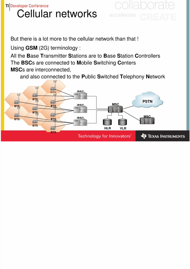
But there is a lot more to the cellular network than that !

Using GSM (2G) terminology :

All the Base Transmitter Stations are to Base Station Controllers

The BSCs are connected to Mobile Switching Centers

MSCs are interconnected,

and also connected to the Public Switched Telephony Network

PSTN

MSC

BTS

BTS

BTS

BTS

BTS

BTS

BTSBTS

BTS

BSC

BSC

BSC

MSC

HLR VLR



Cellular backhauling

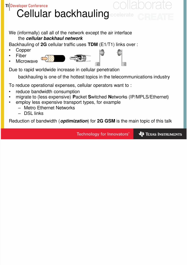
We (informally) call all of the network except the air interfacethe cellular backhaul network

Backhauling of 2G cellular traffic uses TDM (E1/T1) links over :• Copper• Fiber• Microwave

Due to rapid worldwide increase in cellular penetration

backhauling is one of the hottest topics in the telecommunications industry

To reduce operational expenses, cellular operators want to :

• reduce bandwidth consumption

• migrate to (less expensive) Packet Switched Networks (IP/MPLS/Ethernet)• employ less expensive transport types, for example

– Metro Ethernet Networks – DSL links

Reduction of bandwidth (optimization ) for 2G GSM is the main topic of this talk



Cellular backhaul optimization

Voice traffic is already compressed by the mobile station

So why can cellular traffic be optimized at all ?

• TDM transport mechanisms can not reduce bandwidth

• standard user traffic (TRAU) formats are extremely inefficient

• nonactive user channels are sent

• silence/idle frames in active channels are sent

• signaling channels (HDLC-based) are inefficient

• data can be compressed by lossless data compression

• additional mechanisms (e.g. stronger compression) may sometimes be used

ACE-3xxx



Cellular backhaul transport

When TDM transport (e.g. E1 links) is used – optimization enables use of fewer E1s

to carry the same amount of user traffic

– reduced operational expense at dense portions of network

– however, compressed traffic formats are not standardized

When TDM transport is replaced with Packet Switched Networks

– service less expensive to begin with

– service often charged by bandwidth used

–

optimization enables using only the minimum BW needed – operational expense reduced



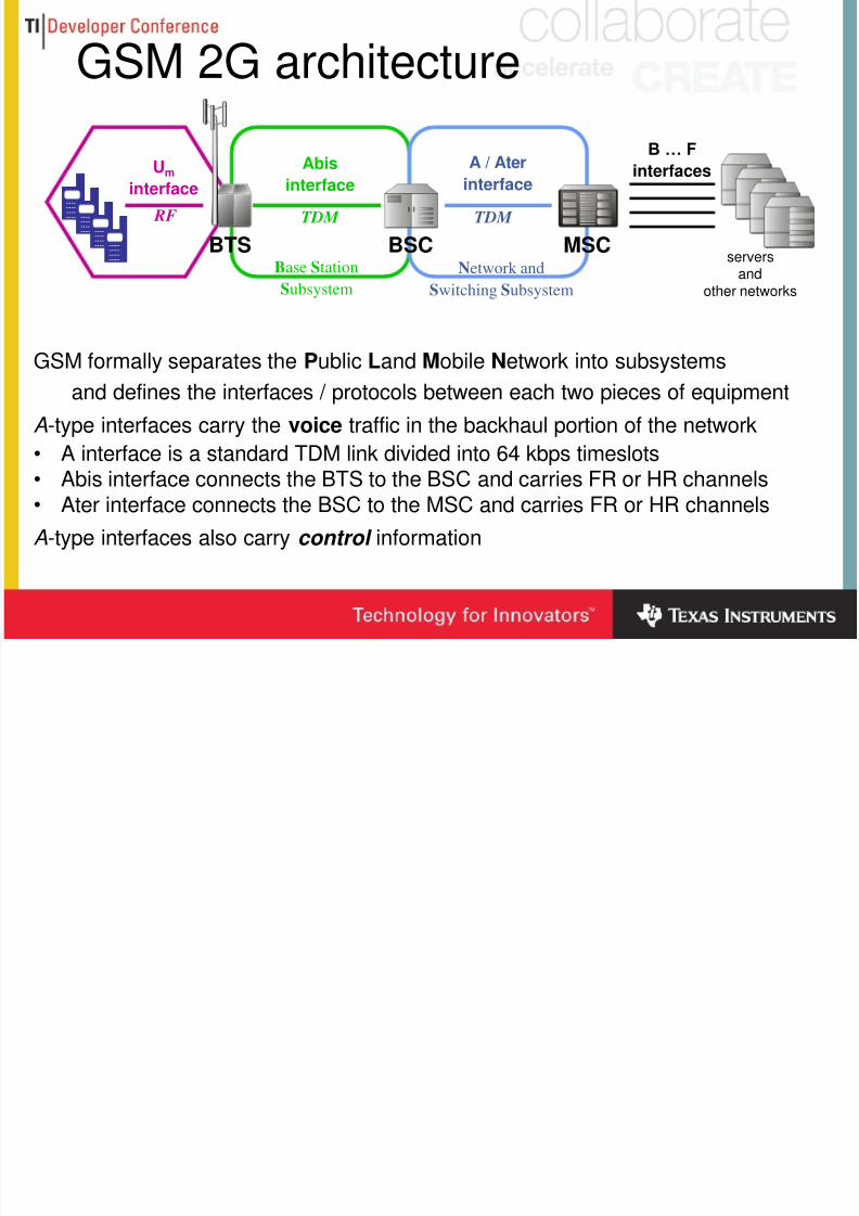
GSM 2G architecture

GSM formally separates the Public Land Mobile Network into subsystems

and defines the interfaces / protocols between each two pieces of equipment

A-type interfaces carry the voice traffic in the backhaul portion of the network

• A interface is a standard TDM link divided into 64 kbps timeslots• Abis interface connects the BTS to the BSC and carries FR or HR channels• Ater interface connects the BSC to the MSC and carries FR or HR channels

A-type interfaces also carry control information

BTS BSC MSCBase Station

Subsystem

Network and

Switching Subsystem

Um

interface

Abis

interface

A / Ater

interface

B … F interfaces

RF TDM TDM

serversand

other networks



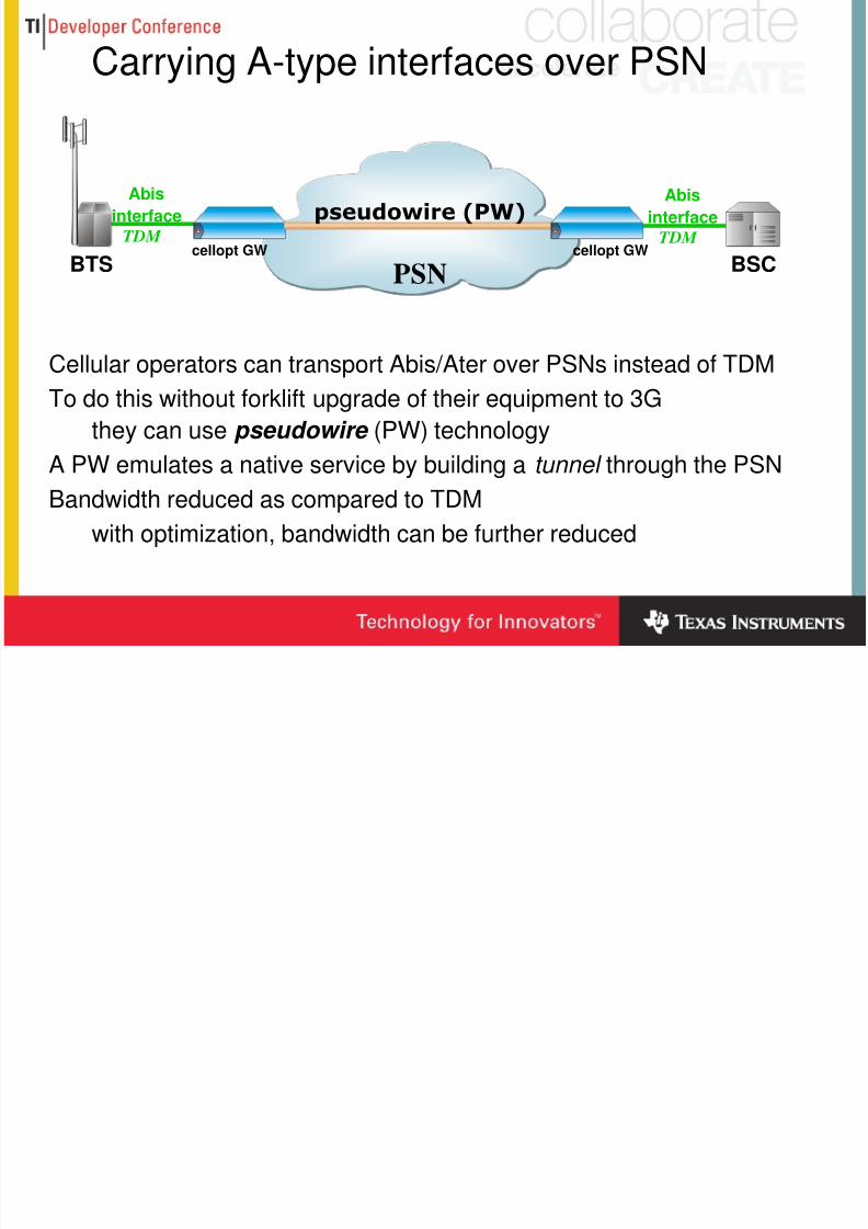
Carrying A-type interfaces over PSN

Cellular operators can transport Abis/Ater over PSNs instead of TDM

To do this without forklift upgrade of their equipment to 3G

they can use pseudowire (PW) technology

A PW emulates a native service by building a tunnel through the PSN

Bandwidth reduced as compared to TDM

with optimization, bandwidth can be further reduced

BTS BSC

Abis

interfaceTDM

Abis

interfaceTDM

PSN

pseudowire (PW)

cellopt GW cellopt GW



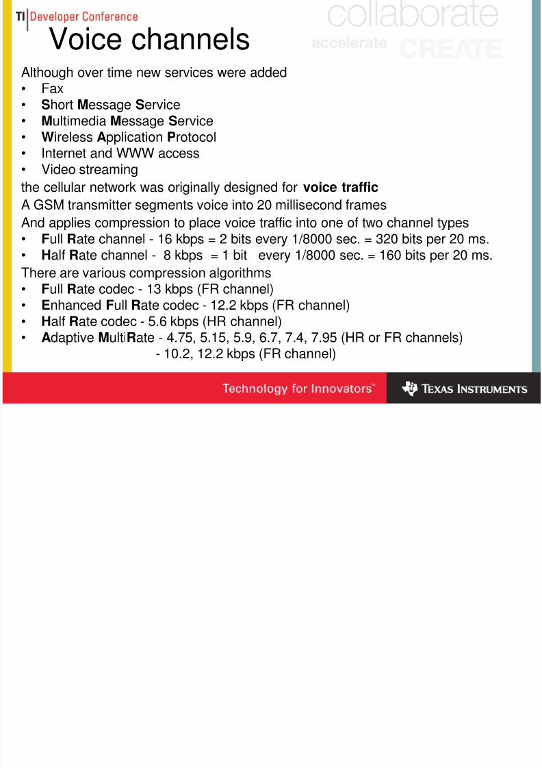
Voice channelsAlthough over time new services were added•

Fax• Short Message Service• Multimedia Message Service• Wireless Application Protocol• Internet and WWW access• Video streaming

the cellular network was originally designed for voice trafficA GSM transmitter segments voice into 20 millisecond frames

And applies compression to place voice traffic into one of two channel types• Full Rate channel - 16 kbps = 2 bits every 1/8000 sec. = 320 bits per 20 ms.• Half Rate channel - 8 kbps = 1 bit every 1/8000 sec. = 160 bits per 20 ms.

There are various compression algorithms

• Full Rate codec - 13 kbps (FR channel)• Enhanced Full Rate codec - 12.2 kbps (FR channel)

• Half Rate codec - 5.6 kbps (HR channel)• Adaptive MultiRate - 4.75, 5.15, 5.9, 6.7, 7.4, 7.95 (HR or FR channels)

- 10.2, 12.2 kbps (FR channel)



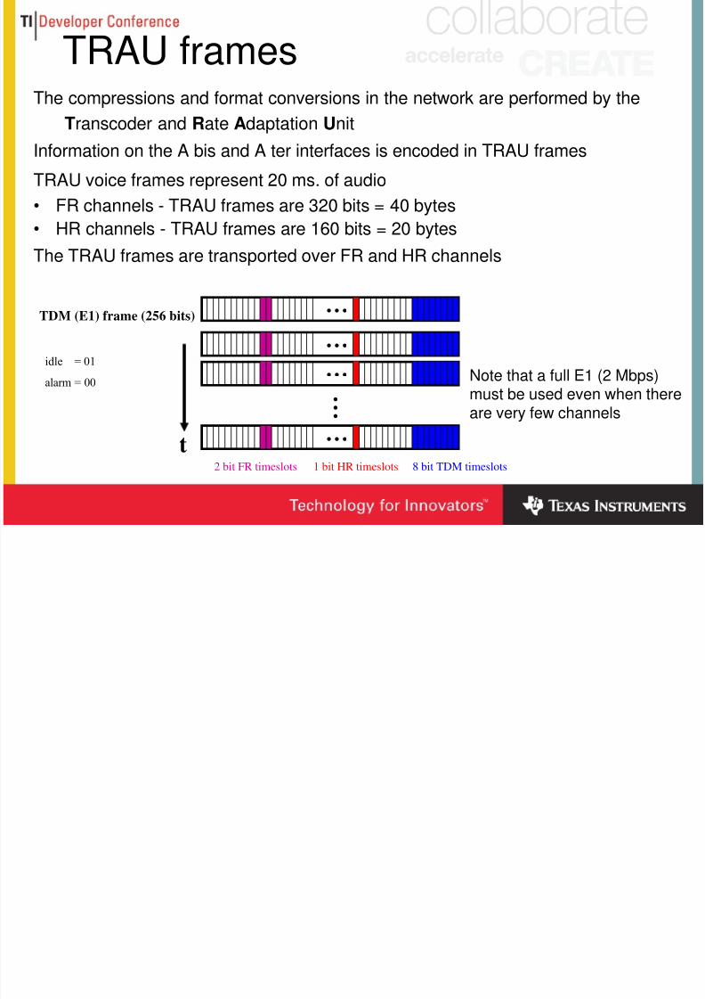
TRAU framesThe compressions and format conversions in the network are performed by the

Transcoder and Rate Adaptation UnitInformation on the A bis and A ter interfaces is encoded in TRAU frames

TRAU voice frames represent 20 ms. of audio

• FR channels - TRAU frames are 320 bits = 40 bytes

• HR channels - TRAU frames are 160 bits = 20 bytes

The TRAU frames are transported over FR and HR channels

…

…

…

...

TDM (E1) frame (256 bits)

t8 bit TDM timeslots1 bit HR timeslots2 bit FR timeslots

…

Note that a full E1 (2 Mbps)must be used even when thereare very few channels

idle = 01

alarm = 00



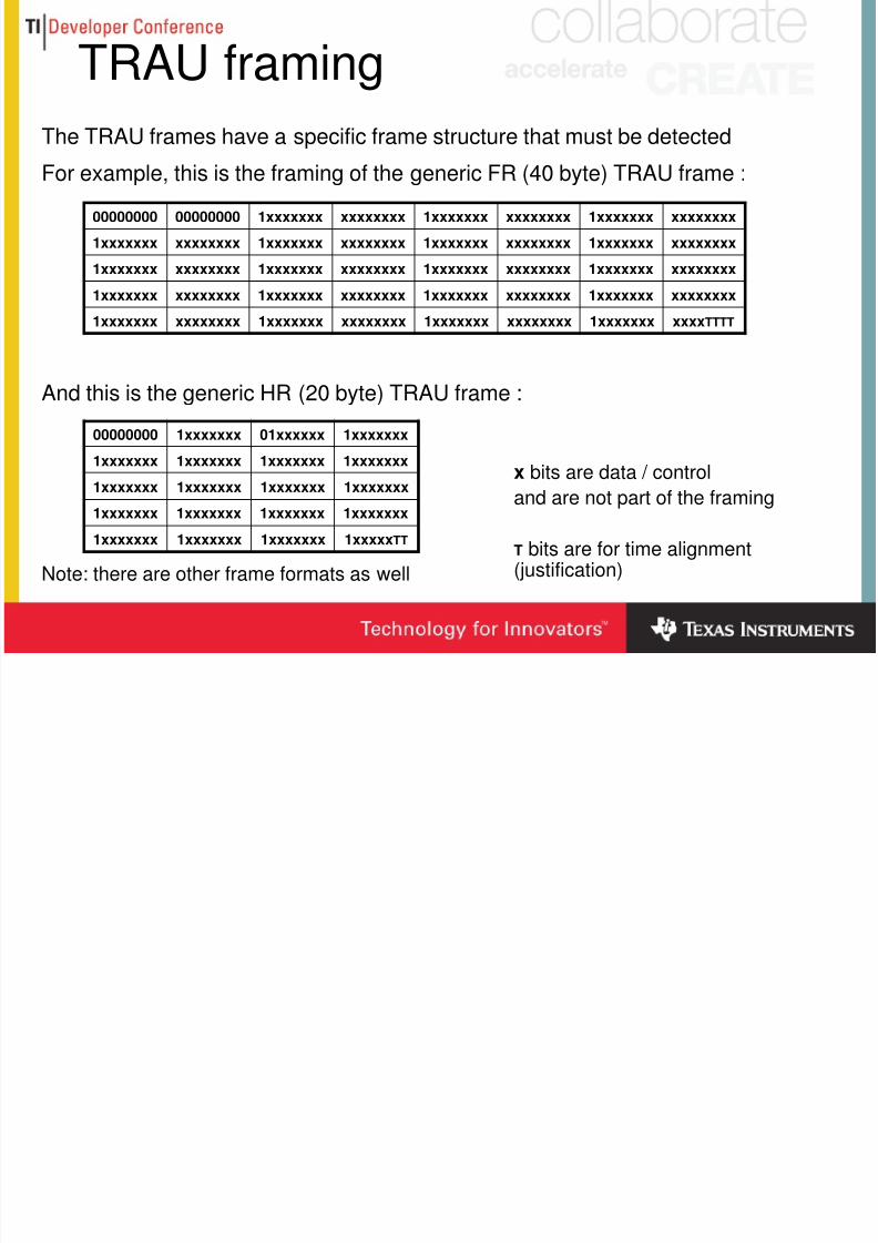
TRAU framing

The TRAU frames have a specific frame structure that must be detected

For example, this is the framing of the generic FR (40 byte) TRAU frame :

And this is the generic HR (20 byte) TRAU frame :

Note: there are other frame formats as well

00000000 00000000 1xxxxxxx xxxxxxxx 1xxxxxxx xxxxxxxx 1xxxxxxx xxxxxxxx

1xxxxxxx xxxxxxxx 1xxxxxxx xxxxxxxx 1xxxxxxx xxxxxxxx 1xxxxxxx xxxxxxxx



1xxxxxxx xxxxxxxx 1xxxxxxx xxxxxxxx 1xxxxxxx xxxxxxxx 1xxxxxxx xxxxTTTT

00000000 1xxxxxxx 01xxxxxx 1xxxxxxx

1xxxxxxx 1xxxxxxx 1xxxxxxx 1xxxxxxx



1xxxxxxx 1xxxxxxx 1xxxxxxx 1xxxxxTT

x bits are data / control

and are not part of the framing

T bits are for time alignment(justification)



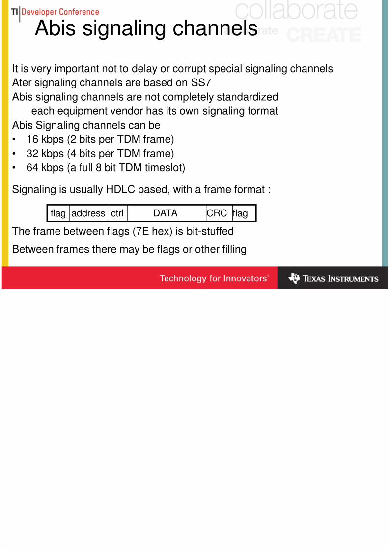
Abis signaling channels

It is very important not to delay or corrupt special signaling channelsAter signaling channels are based on SS7

Abis signaling channels are not completely standardized

each equipment vendor has its own signaling format

Abis Signaling channels can be

• 16 kbps (2 bits per TDM frame)• 32 kbps (4 bits per TDM frame)

• 64 kbps (a full 8 bit TDM timeslot)

Signaling is usually HDLC based, with a frame format :

The frame between flags (7E hex) is bit-stuffed

Between frames there may be flags or other filling

flag address ctrl DATA CRC flag



Backhauling data

User data can be transported over the Abis interface in various ways

Low rate data (up to 9.6 or 14.4 kbps) is transported in TRAU frames

Intermediate rates (up to 114 kbps) are available via GPRS (2.5G)

Higher rates (theoretically up to 384 kbps) via EDGE (2.75G)

GPRS / EDGE are carried over G-type interfaceswhich may share the same TDM link as A-type interfaces

GPRS/EDGE bandwidth allocation may be dynamic

it takes over bits not used by the A-type interfaces

In 3G networks data can be much higher rate (over 2 Mbps, e.g. 10 Mbps)

carried over I-type interfacesthat use separate transport media



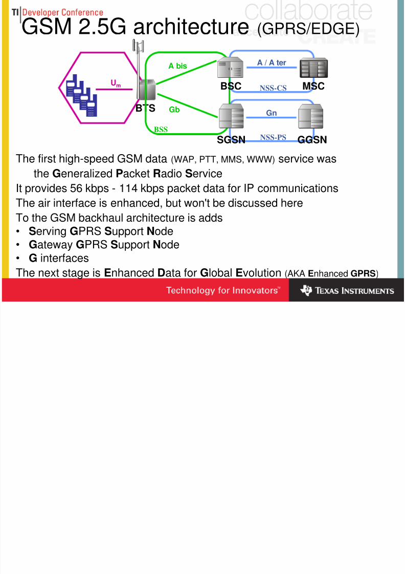
GSM 2.5G architecture (GPRS/EDGE)

The first high-speed GSM data (WAP, PTT, MMS, WWW) service was

the Generalized Packet Radio Service

It provides 56 kbps - 114 kbps packet data for IP communications

The air interface is enhanced, but won't be discussed here

To the GSM backhaul architecture is adds• Serving GPRS Support Node• Gateway GPRS Support Node• G interfaces

The next stage is Enhanced Data for Global Evolution (AKA Enhanced GPRS)

BTS

MSCUm

A bis A / A ter

BSC

Gb

BSS

SGSN

Gn

NSS-CS

GGSNNSS-PS



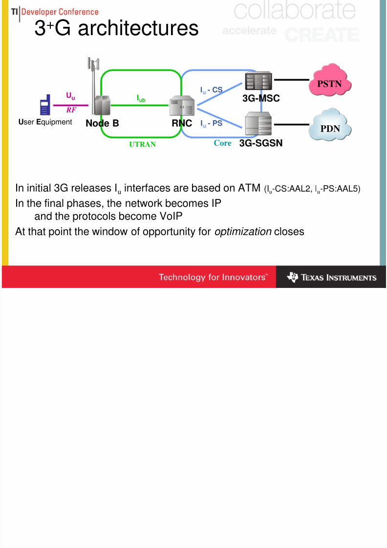
3+G architectures

In initial 3G releases Iu interfaces are based on ATM (Iu-CS:AAL2, Iu-PS:AAL5)

In the final phases, the network becomes IPand the protocols become VoIP

At that point the window of opportunity for optimization closes

Node B RNC

Uu Iub

Iu - CS

RF

User Equipment

3G-MSC

3G-SGSN

Iu - PSPDN

PSTN

UTRAN Core



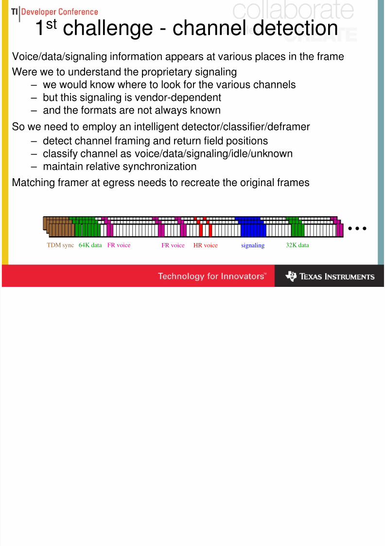
1st challenge - channel detectionVoice/data/signaling information appears at various places in the frame

Were we to understand the proprietary signaling – we would know where to look for the various channels – but this signaling is vendor-dependent – and the formats are not always known

So we need to employ an intelligent detector/classifier/deframer

– detect channel framing and return field positions – classify channel as voice/data/signaling/idle/unknown – maintain relative synchronization

Matching framer at egress needs to recreate the original frames

signalingHR voiceFR voice64K dataTDM sync FR voice 32K data

…



Channel detector/classifierThis detector/classifier needs to continually scan all

• 1-bit positions for HR TRAU frames• even aligned 2-bit fields for FR TRAU frames• even aligned 2-bit fields for HDLC• nibble-aligned nibbles for HDLC• byte-aligned octets for HDLC•

fields of idle bits• anything else

and then return the identifications and positions found

Unidentified non-idle information must be reliably transported

The processing involves

• searching for specific bit combinations• performing bit correlations

and is extremely computationally intensive

Can be performed by a DSP with good bit-oriented operations



2nd challenge - optimization

Once the various components have been foundthe information needs to be reduced in size and reliably transported

• Idle fields need not be sent, often accounting for a large BW reduction

• TRAU framing overhead may be removed

• Voice frames marked as silent (DTX) may be suppressed• Voice Activity Detection may be employed to suppress silence

• HDLC flags are removed and the contents destuffed

• Data may be compressed

We will deal with each of these in turn



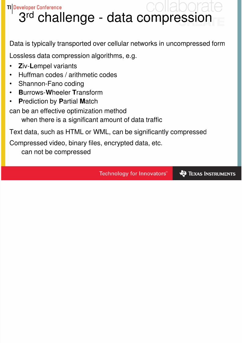
3rd challenge - data compression

Data is typically transported over cellular networks in uncompressed form

Lossless data compression algorithms, e.g.

• Ziv-Lempel variants

• Huffman codes / arithmetic codes

• Shannon-Fano coding• Burrows-Wheeler Transform

• Prediction by Partial Match

can be an effective optimization method

when there is a significant amount of data traffic

Text data, such as HTML or WML, can be significantly compressed

Compressed video, binary files, encrypted data, etc.

can not be compressed



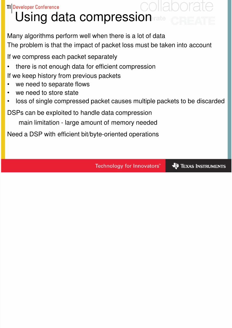
Using data compression

Many algorithms perform well when there is a lot of data

The problem is that the impact of packet loss must be taken into account

If we compress each packet separately

• there is not enough data for efficient compression

If we keep history from previous packets

• we need to separate flows

• we need to store state

• loss of single compressed packet causes multiple packets to be discarded

DSPs can be exploited to handle data compression

main limitation - large amount of memory needed

Need a DSP with efficient bit/byte-oriented operations



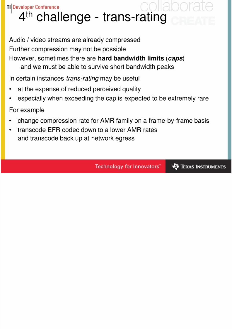
4th challenge - trans-rating

Audio / video streams are already compressedFurther compression may not be possible

However, sometimes there are hard bandwidth limits (caps )

and we must be able to survive short bandwidth peaks

In certain instances trans-rating may be useful

• at the expense of reduced perceived quality

• especially when exceeding the cap is expected to be extremely rare

For example

• change compression rate for AMR family on a frame-by-frame basis• transcode EFR codec down to a lower AMR rates

and transcode back up at network egress



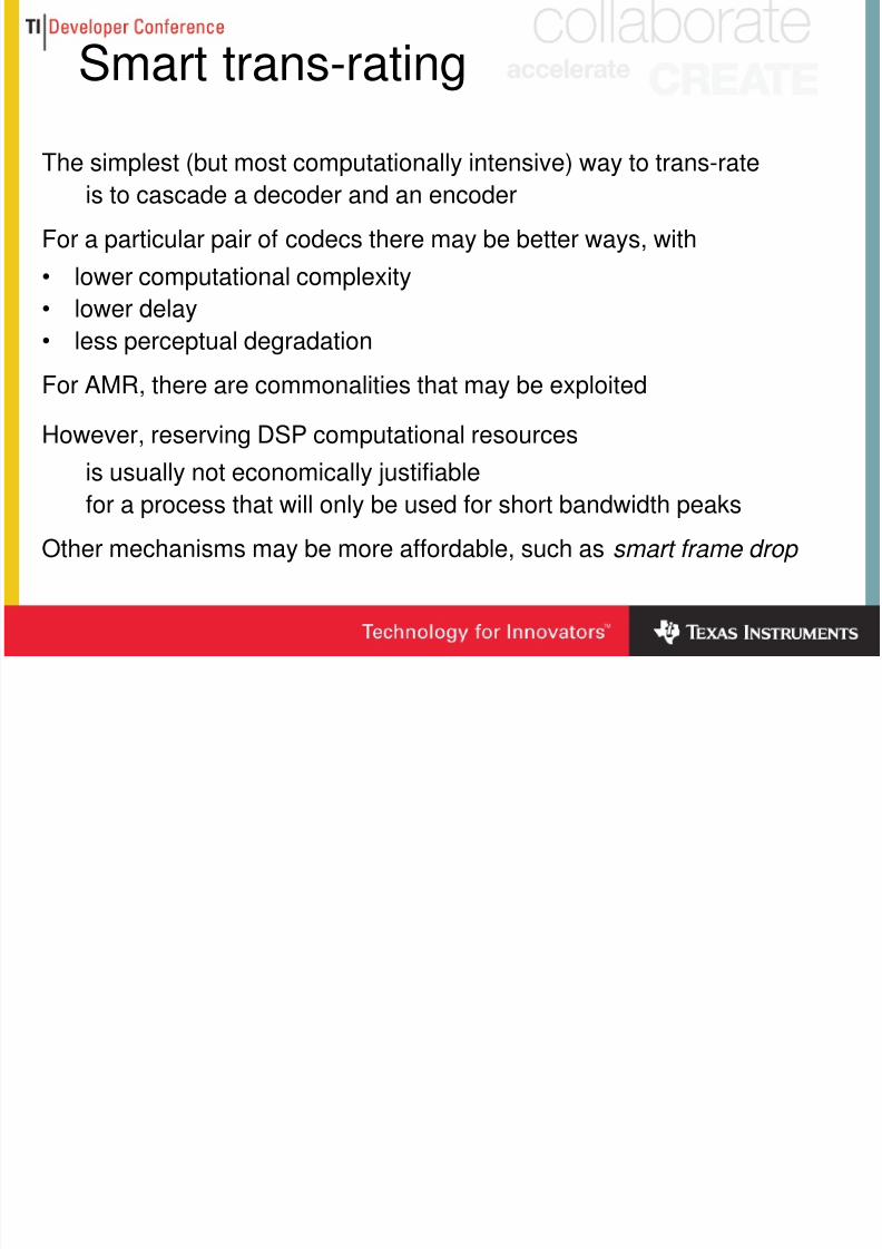
Smart trans-rating

The simplest (but most computationally intensive) way to trans-rateis to cascade a decoder and an encoder

For a particular pair of codecs there may be better ways, with

• lower computational complexity

• lower delay• less perceptual degradation

For AMR, there are commonalities that may be exploited

However, reserving DSP computational resources

is usually not economically justifiable

for a process that will only be used for short bandwidth peaks

Other mechanisms may be more affordable, such as smart frame drop



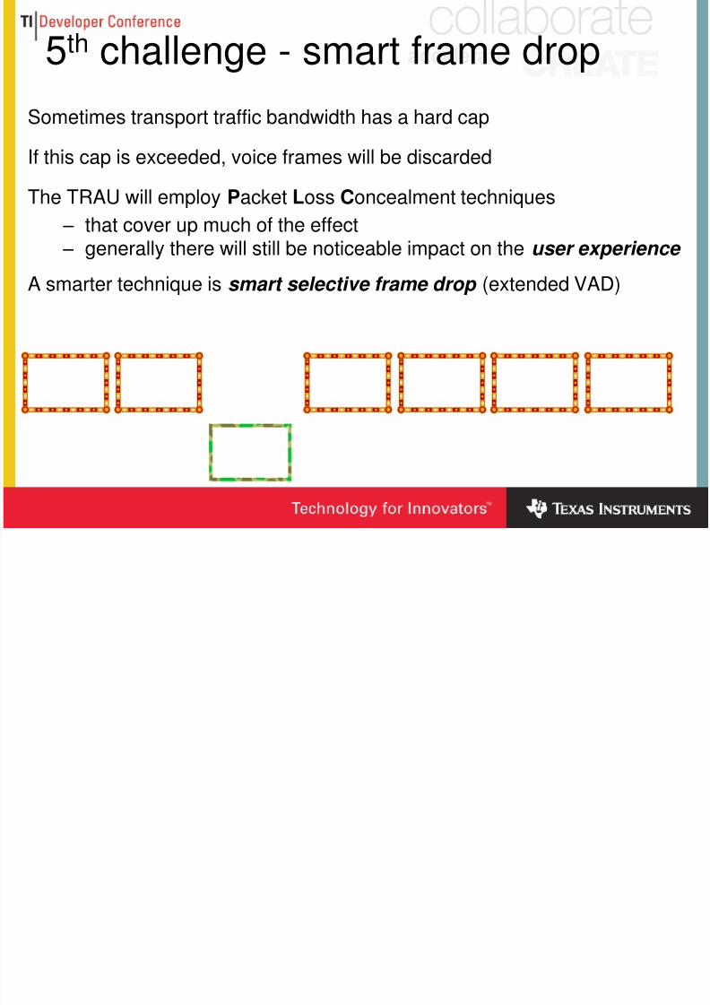
5th challenge - smart frame drop

Sometimes transport traffic bandwidth has a hard capIf this cap is exceeded, voice frames will be discarded

The TRAU will employ Packet Loss Concealment techniques

– that cover up much of the effect

– generally there will still be noticeable impact on the user experience

A smarter technique is smart selective frame drop (extended VAD)



Smart frame drop

Instead of dropping randomly chosen voice frames … we can carefully select the frames to dropusing a criterion of least perceptual quality degradation

The selection can be based on voice parameters in the TRAU frame

without full decoding of the voice coding

The resulting DSP code

• is codec-dependent• requires saving of state information per channel• but does not require large amounts of memory

The smart frame drop mechanismshould be tightly coupled controlled to the main control functionso that only the minimal percentage of frames are dropped



6th challenge - timing recovery

TDM's physical layer transfers accurate frequency (sync) informationGSM BTSs use the accurate frequency recovered from the TDM link to

• generate accurate radio frequencies

• generate symbol timing

• send time offset information to mobile stations

• ensure short handover when moving from cell to cellCDMA and 3G cellular systems also need accurate Time Of Day

Requirements are stringent :

• absolute frequency accuracy must be better than 50 ppb

• jitter and wander need to conform to ITU TDM standards

• 3G stations need time accuracy of better than 3 s• 3G TDD mode requires time accuracy of better than 1.25 s from UTC

When replacing TDM links with PWs over PSNs we lose timing information



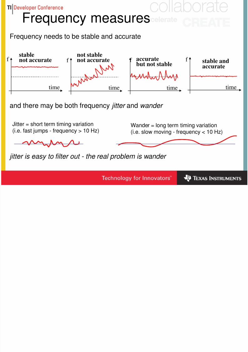
Frequency measuresFrequency needs to be stable and accurate

and there may be both frequency jitter and wander

jitter is easy to filter out - the real problem is wander

f f

time

f

time

f

timetime

stablenot accurate

not stablenot accurate accurate

but not stablestable andaccurate

Jitter = short term timing variation

(i.e. fast jumps - frequency > 10 Hz)

Wander = long term timing variation

(i.e. slow moving - frequency < 10 Hz)



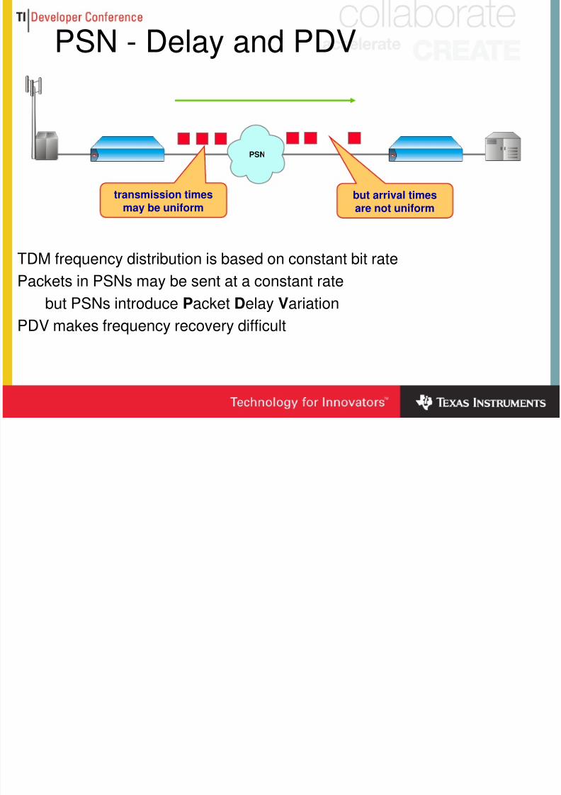
PSN - Delay and PDV

TDM frequency distribution is based on constant bit rate

Packets in PSNs may be sent at a constant rate

but PSNs introduce Packet Delay Variation

PDV makes frequency recovery difficult

PSN

but arrival timesare not uniform transmission timesmay be uniform



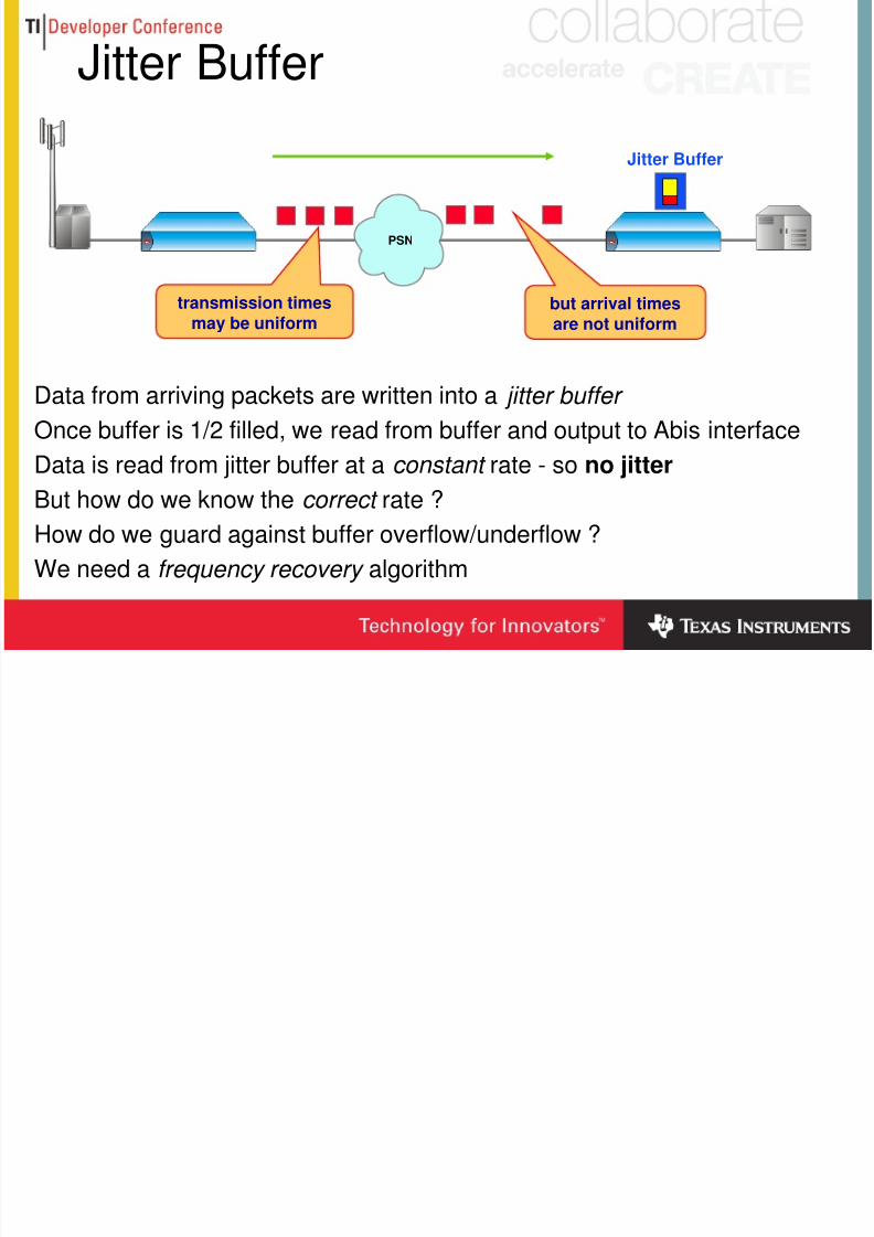
Jitter Buffer

Data from arriving packets are written into a jitter buffer

Once buffer is 1/2 filled, we read from buffer and output to Abis interface

Data is read from jitter buffer at a constant rate - so no jitterBut how do we know the correct rate ?

How do we guard against buffer overflow/underflow ?

We need a frequency recovery algorithm

Jitter Buffer

PSN

but arrival timesare not uniform transmission timesmay be uniform



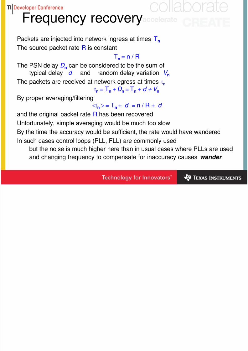
Frequency recovery

Packets are injected into network ingress at times Tn

The source packet rate R is constant

Tn = n / R

The PSN delay D n can be considered to be the sum oftypical delay d and random delay variation V n

The packets are received at network egress at times tntn = Tn + D n = Tn + d + V n

By proper averaging/filtering<tn > = Tn + d = n / R + d

and the original packet rate R has been recovered

Unfortunately, simple averaging would be much too slow

By the time the accuracy would be sufficient, the rate would have wanderedIn such cases control loops (PLL, FLL) are commonly used

but the noise is much higher here than in usual cases where PLLs are used

and changing frequency to compensate for inaccuracy causes wander



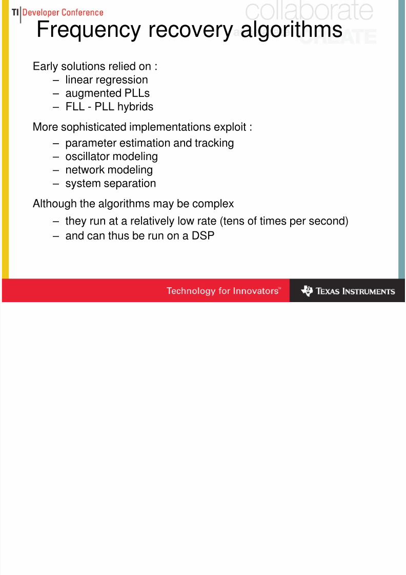
Frequency recovery algorithms

Early solutions relied on : – linear regression – augmented PLLs – FLL - PLL hybrids

More sophisticated implementations exploit :

– parameter estimation and tracking – oscillator modeling – network modeling – system separation

Although the algorithms may be complex

– they run at a relatively low rate (tens of times per second)

– and can thus be run on a DSP



SummaryCellular backhaul optimization enables

– more efficient use of overloaded transport infrastructures – lowering of OPEX

Cellular optimization is applicable to 2G and 2.5G networks

There are many challenges to building an operational system

– channel detection, classification, and deframing – packet-loss-tolerant data compression

– smart trans-rating

– smart selective frame drop

–timing recovery

DSPs provide a good platform for meeting these challenges

For more information, visit www.RAD.com

Documents

Cellular Back Hauling Optimization