PLANNING AND OPTIMIZATION OF CELLULAR

HETEROGENEOUS NETWORKS

A Thesis

Submitted to the Faculty of Graduate Studies and Research

In Partial Fulfillment of the Requirements

For the Degree of

Doctor of Philosophy

in

Electronic Systems Engineering

University of Regina

by

Diego Alberto Castro-Hernandez

Regina, Saskatchewan

December 2016

Copyright 2016: D. A. Castro-Hernandez

UNIVERSITY OF REGINA

FACULTY OF GRADUATE STUDIES AND RESEARCH

SUPERVISORY AND EXAMINING COMMITTEE

Diego Alberto Castro-Hernandez, candidate for the degree of Doctor of Philosophy in Electronic Systems Engineering, has presented a thesis titled, Planning and Optimization of Cellular Heterogeneous Networks, in an oral examination held on October 4, 2016. The following committee members have found the thesis acceptable in form and content, and that the candidate demonstrated satisfactory knowledge of the subject material. External Examiner: *Dr. Anthony Soong, Huawei Technologies

Supervisor: Dr. Raman Paranjape, Electronic Systems Engineering

Committee Member: Dr. Craig Gelowitz, Software Systems Engineering

Committee Member: Dr. Paul Laforge, Electronic Systems Engineering

Committee Member: Dr. David Gerhard, Department of Computer Science

Chair of Defense: Dr. Remus Floricel, Department of Mathematics and Statistics *Via teleconference

Abstract

Over the past few years there has been an dramatic increase in mobile data traffic

demand, a trend that is expected to continue in coming years. Traditional macrocell-

only networks are incapable of providing the quality of service that modern subscribers

expect from a mobile broadband service. Increasing network densification with the

deployment of low power base stations has proven to be an effective solution in this

regard. The resulting multi-tier topology is known as heterogeneous networks or

HetNets. This new topology brings a series of new and important challenges, since

traditional practices applied for macrocell-only networks no longer provide optimal

results. There is a need to increase the understanding about the operation of these

systems and develop new techniques to properly plan, design and optimize HetNets.

These new techniques should focus on the efficient use of resources during network

planning, reducing costs of deployments, and facilitating the configuration and main-

tenance of HetNets. This thesis has focused on exploring novel solutions to challenges

in two main areas regarding the operation of HetNets: planning and self-optimization.

Regarding the planning of HetNets, the thesis starts by treating the issue of im-

proving the accuracy of site-specific path loss prediction models for outdoor microcell

deployments. The prediction of coverage areas based on path loss estimations are

essential for network operators during the planning and design of new deployments.

The thesis proposes two novel tuning algorithms intended to optimize the propagation

model parameters based on information from a limited set of physical measurements.

Also in the area of network planning, it is fundamental for network operators

to understand typical user mobility patterns and accurately estimate the quality of

the service as users move. For this purpose system level simulations are typically

carried out. This thesis proposes a downlink system level simulator that incorporates

ii

a mobility model as well as a traffic model where users are categorized according to

their type of demand. We were able to demonstrate that an appropriate traffic model

can significantly increase the accuracy in the estimation of the the user experience.

Regarding the self-optimization of HetNets, the thesis treats two key challenges:

load balancing and the optimization of handover parameters. Proper load balanc-

ing among base stations is fundamental in order to leverage the benefits in network

capacity that HetNets can provide. In this thesis a novel and practical load balanc-

ing algorithm is proposed. With this algorithm, each base station can solve locally

a load-aware utility maximization problem. As opposed to current approaches, the

algorithm minimizes the required level of coordination among base stations, hence

reducing the impact on the signaling load of the network and potentially reducing

the effect on power consumption.

Finally, the thesis proposes a novel methodology to optimize handover parameters

for in-building systems. The goal of the methodology is to minimize handover failures

and the triggering of unnecessary handovers, while maximizing the quality of service

provided to users approaching the cell-edge. With this methodology, a base station

can customize the handover parameters according to the current load level and the

specific radio frequency conditions of the cell-edge that a user will experience as it

moves out of the service area.

With the research work described in this thesis, we have expanded the understand-

ing about the operation of HetNets. The algorithms and methodologies proposed in

this thesis have the overall objective of maximizing the benefits that HetNets can

provide through the efficient use and coordination of the resources in every tier.

iii

Acknowledgements

I am truly grateful to my advisor Dr. Raman Paranjape, for his trust, help and

support throughout my years as a graduate student. I thank Dr. Paranjape for his

guidance, not only for providing me with valuable academic advice but also encour-

aging me to become a better professional.

I acknowledge the technical assistance and financial support provided by SaskTel

Inc. In particular, I thank the members of the Wireless Network Support team,

particularly Marc Ell, Peter Dang and Edward Steward. I am very grateful to Ed for

providing his time and dedication to assist with the collection and post-processing of

experimental data.

I thank the Faculty of Graduate Studies and Research as well as the University

of Regina for providing financial support through research awards, scholarships and

assistantships.

I thank my fellow graduate students that were part of this journey at one point

or another, in particular Zhanle Wang, Maryam Alizadeh and Sean Cau.

I am deeply grateful to Lena for her love, patience and support during the ups

and downs of the life as graduate student.

Last but not least, it is hard for me to find the words to express my gratitude to

my parents, what I am today is due to their hard work and love. It has been hard

to be far away from them during these years, but I am deeply grateful as they have

been there for me every step of the way. I thank my siblings Kattia and Luis for their

constant support and encouragement from the very beginning of this journey.

iv

Post Defense Acknowledgement

Special thanks to the members of my Ph.D. committee: Dr. Paul Laforge, Dr. Craig

Gelowitz, Dr. David Gerhard and the external examiner of this thesis Dr. Anthony

Soong. The quality of this research work has greatly benefited from their valuable

advise.

v

Dedication

To Myriam and Eliecer,

my loving parents

vi

Table of Contents

Abstract . . . . . . . . . . . . . . . . . . . . . . . . . . . . . . . . . . . . . . ii

Acknowledgements . . . . . . . . . . . . . . . . . . . . . . . . . . . . . . . iv

Post Defense Acknowledgement . . . . . . . . . . . . . . . . . . . . . . . v

Dedication . . . . . . . . . . . . . . . . . . . . . . . . . . . . . . . . . . . . . vi

List of Tables . . . . . . . . . . . . . . . . . . . . . . . . . . . . . . . . . . . xi

List of Figures . . . . . . . . . . . . . . . . . . . . . . . . . . . . . . . . . . xii

List of Abbreviations . . . . . . . . . . . . . . . . . . . . . . . . . . . . . . xiv

Chapter 1Introduction . . . . . . . . . . . . . . . . . . . . . . . . . . . . . . . . . . 11.1 Heterogeneous networks . . . . . . . . . . . . . . . . . . . . . . . . . 21.2 Challenges in HetNets . . . . . . . . . . . . . . . . . . . . . . . . . . 4

1.2.1 Planning and design of outdoor HetNets . . . . . . . . . . . . 51.2.2 Assessment of quality of service during network planning . . . 71.2.3 Cell association and load balancing . . . . . . . . . . . . . . . 91.2.4 Self-optimizing networks . . . . . . . . . . . . . . . . . . . . . 11

1.3 Contributions . . . . . . . . . . . . . . . . . . . . . . . . . . . . . . . 151.4 Organization of the thesis . . . . . . . . . . . . . . . . . . . . . . . . 18

Chapter 2Local tuning of a site-specific propagation path loss model for

microcell environments . . . . . . . . . . . . . . . . . . . . . 202.1 Introduction . . . . . . . . . . . . . . . . . . . . . . . . . . . . . . . . 202.2 Related work . . . . . . . . . . . . . . . . . . . . . . . . . . . . . . . 242.3 Path loss prediction model . . . . . . . . . . . . . . . . . . . . . . . . 26

2.3.1 Free space propagation . . . . . . . . . . . . . . . . . . . . . . 292.3.2 Over-rooftop and vertical-edge diffractions . . . . . . . . . . . 292.3.3 Reflections . . . . . . . . . . . . . . . . . . . . . . . . . . . . . 312.3.4 Scattering losses due to foliage . . . . . . . . . . . . . . . . . . 312.3.5 Propagation path loss . . . . . . . . . . . . . . . . . . . . . . 322.3.6 Model parameters . . . . . . . . . . . . . . . . . . . . . . . . . 33

2.4 Global, Semi-global and Local tuning . . . . . . . . . . . . . . . . . . 342.4.1 Global tuning based on LSE . . . . . . . . . . . . . . . . . . . 352.4.2 Semi-global tuning . . . . . . . . . . . . . . . . . . . . . . . . 352.4.3 Local tuning . . . . . . . . . . . . . . . . . . . . . . . . . . . . 37

vii

2.4.3.1 Practical considerations . . . . . . . . . . . . . . . . 392.5 Gathering of experimental data . . . . . . . . . . . . . . . . . . . . . 402.6 Results & Discussion . . . . . . . . . . . . . . . . . . . . . . . . . . . 42

2.6.1 Evaluating the accuracy of the tuned model . . . . . . . . . . 422.6.2 Distribution of the prediction error . . . . . . . . . . . . . . . 462.6.3 Influence of the size of the training set . . . . . . . . . . . . . 47

2.7 Summary . . . . . . . . . . . . . . . . . . . . . . . . . . . . . . . . . 48

Chapter 3Walk/Speed test simulator for cellular network planning . . . . . . 503.1 Introduction . . . . . . . . . . . . . . . . . . . . . . . . . . . . . . . . 503.2 Related work . . . . . . . . . . . . . . . . . . . . . . . . . . . . . . . 533.3 LTE/LTE-A Downlink Simulator . . . . . . . . . . . . . . . . . . . . 55

3.3.1 Overview of the simulator . . . . . . . . . . . . . . . . . . . . 563.3.2 Propagation path loss predictions . . . . . . . . . . . . . . . . 583.3.3 Spatial Distribution of mobile users . . . . . . . . . . . . . . . 593.3.4 Mobility models . . . . . . . . . . . . . . . . . . . . . . . . . . 593.3.5 Traffic models . . . . . . . . . . . . . . . . . . . . . . . . . . . 603.3.6 Scheduler . . . . . . . . . . . . . . . . . . . . . . . . . . . . . 613.3.7 Mobility Management . . . . . . . . . . . . . . . . . . . . . . 633.3.8 Updating state of UEs after each TTI . . . . . . . . . . . . . . 64

3.4 Collection of experimental data . . . . . . . . . . . . . . . . . . . . . 643.5 Results & Analysis . . . . . . . . . . . . . . . . . . . . . . . . . . . . 67

3.5.1 RSRP and SINR estimations . . . . . . . . . . . . . . . . . . . 673.5.2 Downlink data rate . . . . . . . . . . . . . . . . . . . . . . . . 67

3.6 Summary . . . . . . . . . . . . . . . . . . . . . . . . . . . . . . . . . 71

Chapter 4A Distributed Load Balancing Algorithm for Heterogeneous Net-

works . . . . . . . . . . . . . . . . . . . . . . . . . . . . . . . . 724.1 Introduction . . . . . . . . . . . . . . . . . . . . . . . . . . . . . . . . 734.2 Related work . . . . . . . . . . . . . . . . . . . . . . . . . . . . . . . 754.3 System model . . . . . . . . . . . . . . . . . . . . . . . . . . . . . . . 78

4.3.1 Load of eNBs . . . . . . . . . . . . . . . . . . . . . . . . . . . 804.4 Problem formulation and description of load balancing algorithms . . 81

4.4.1 Load balancing algorithm based on local optimization (LOM) 824.4.2 Algorithm based on the Subgradient Method (SGM) . . . . . 854.4.3 Algorithm based on Dual Coordinate Descend (DCD) . . . . 87

4.5 Performance evaluation . . . . . . . . . . . . . . . . . . . . . . . . . . 884.5.1 Distribution of users . . . . . . . . . . . . . . . . . . . . . . . 894.5.2 Distribution of the load among eNBs . . . . . . . . . . . . . . 904.5.3 Cumulative distribution of the normalized long-term rate . . . 914.5.4 Evaluation of the practicality of the algorithms . . . . . . . . 92

4.6 Summary . . . . . . . . . . . . . . . . . . . . . . . . . . . . . . . . . 93

viii

Chapter 5Classification of user trajectories in HetNets using unsupervised-

shapelets and multi-resolution wavelet decomposition . . 955.1 Introduction . . . . . . . . . . . . . . . . . . . . . . . . . . . . . . . . 96

5.1.1 Cell-edge characterization . . . . . . . . . . . . . . . . . . . . 975.1.2 Mobility robustness optimization in SON . . . . . . . . . . . . 985.1.3 Load balancing optimization . . . . . . . . . . . . . . . . . . . 98

5.2 Related work . . . . . . . . . . . . . . . . . . . . . . . . . . . . . . . 995.3 Contributions . . . . . . . . . . . . . . . . . . . . . . . . . . . . . . . 1005.4 Handovers and RSRP measurement reports in LTE/LTE-A systems . 1015.5 Clustering of time series . . . . . . . . . . . . . . . . . . . . . . . . . 103

5.5.1 Shapelets . . . . . . . . . . . . . . . . . . . . . . . . . . . . . 1055.5.2 Generating unsupervised-shapelets . . . . . . . . . . . . . . . 1065.5.3 Clustering using unsupervised-shapelets . . . . . . . . . . . . 1085.5.4 Wavelets and multi-resolution analysis . . . . . . . . . . . . . 1095.5.5 Clustering of time series with multi-resolution analysis and

shapelets . . . . . . . . . . . . . . . . . . . . . . . . . . . . . . 1115.5.6 Automatic determination of the number of clusters . . . . . . 113

5.6 Performance evaluation . . . . . . . . . . . . . . . . . . . . . . . . . . 1175.6.1 Evaluation procedure . . . . . . . . . . . . . . . . . . . . . . . 119

5.7 Summary . . . . . . . . . . . . . . . . . . . . . . . . . . . . . . . . . 124

Chapter 6Optimization of handover parameters for in-building systems . . . 1276.1 Introduction . . . . . . . . . . . . . . . . . . . . . . . . . . . . . . . . 1276.2 Related work . . . . . . . . . . . . . . . . . . . . . . . . . . . . . . . 1296.3 Contributions . . . . . . . . . . . . . . . . . . . . . . . . . . . . . . . 1326.4 Handover procedure in LTE/LTE-A . . . . . . . . . . . . . . . . . . . 1336.5 Description of the methodology . . . . . . . . . . . . . . . . . . . . . 136

6.5.1 Collection of measurement reports . . . . . . . . . . . . . . . . 1396.5.2 Clustering of time series . . . . . . . . . . . . . . . . . . . . . 1406.5.3 Optimization of handover parameters . . . . . . . . . . . . . . 140

6.5.3.1 Formulation of the optimization problem . . . . . . . 1416.5.4 Calculation of performance indicators . . . . . . . . . . . . . . 1436.5.5 Solving the optimization problem . . . . . . . . . . . . . . . . 1466.5.6 Matching of time series . . . . . . . . . . . . . . . . . . . . . . 147

6.6 Experimental setup . . . . . . . . . . . . . . . . . . . . . . . . . . . . 1486.7 Performance evaluation . . . . . . . . . . . . . . . . . . . . . . . . . . 149

6.7.1 Clustering algorithm . . . . . . . . . . . . . . . . . . . . . . . 1506.7.2 HO optimization . . . . . . . . . . . . . . . . . . . . . . . . . 151

6.7.2.1 Data rate gains . . . . . . . . . . . . . . . . . . . . . 1556.7.3 Matching algorithm . . . . . . . . . . . . . . . . . . . . . . . . 157

6.8 Summary . . . . . . . . . . . . . . . . . . . . . . . . . . . . . . . . . 159

ix

Chapter 7Conclusions . . . . . . . . . . . . . . . . . . . . . . . . . . . . . . . . . . 1617.1 Summary . . . . . . . . . . . . . . . . . . . . . . . . . . . . . . . . . 1617.2 Future research directions . . . . . . . . . . . . . . . . . . . . . . . . 166

References . . . . . . . . . . . . . . . . . . . . . . . . . . . . . . . . . . . . . 169

Appendix ASystem level simulator . . . . . . . . . . . . . . . . . . . . . . . . . . . 183A.1 Introduction . . . . . . . . . . . . . . . . . . . . . . . . . . . . . . . . 183A.2 Overview of the simulator . . . . . . . . . . . . . . . . . . . . . . . . 183A.3 Software parameters . . . . . . . . . . . . . . . . . . . . . . . . . . . 183A.4 Model of the physical environment . . . . . . . . . . . . . . . . . . . 185A.5 Network layout . . . . . . . . . . . . . . . . . . . . . . . . . . . . . . 186A.6 Path losses . . . . . . . . . . . . . . . . . . . . . . . . . . . . . . . . . 187A.7 Link abstraction model . . . . . . . . . . . . . . . . . . . . . . . . . . 188A.8 Simulation of TTIs . . . . . . . . . . . . . . . . . . . . . . . . . . . . 189

A.8.1 Scheduler . . . . . . . . . . . . . . . . . . . . . . . . . . . . . 189A.8.2 Updating state of UEs after each TTI . . . . . . . . . . . . . . 190

A.9 Throughput calculation . . . . . . . . . . . . . . . . . . . . . . . . . . 191

Appendix BLoad balancing and adaptive adjustment of the REB . . . . . . . . 192B.1 Introduction . . . . . . . . . . . . . . . . . . . . . . . . . . . . . . . . 192B.2 Adaptive bias adjustment . . . . . . . . . . . . . . . . . . . . . . . . 192B.3 Performance evaluation . . . . . . . . . . . . . . . . . . . . . . . . . . 194

B.3.1 Distribution of users . . . . . . . . . . . . . . . . . . . . . . . 196B.3.2 Fairness of load balancing . . . . . . . . . . . . . . . . . . . . 197B.3.3 Data rate gain evaluation . . . . . . . . . . . . . . . . . . . . 198

B.4 Summary . . . . . . . . . . . . . . . . . . . . . . . . . . . . . . . . . 199

x

List of Tables1.1 Types of small cells based on transmission power . . . . . . . . . . . 3

2.1 Selected test locations for test transmitter . . . . . . . . . . . . . . . 402.2 Overall mean error and mean absolute error, in dB . . . . . . . . . . 43

3.1 Example of traffic categories according to QoS requirements . . . . . 613.2 Example of scheduling probabilities, percentage of users and expected

data rates for each traffic category . . . . . . . . . . . . . . . . . . . . 633.3 Mean error and mean absolute error of RSRP and SINR estimations.

Standard deviation is shown between brackets, all units in dBm . . . 683.4 Mean error and mean absolute error of data rate estimations. Standard

deviation is shown between brackets, all units in Mbps . . . . . . . . 71

5.1 Calculation of Rand index . . . . . . . . . . . . . . . . . . . . . . . . 1125.2 Simulation parameters . . . . . . . . . . . . . . . . . . . . . . . . . . 1185.3 Accuracy of the selected number of clusters . . . . . . . . . . . . . . . 123

6.1 Parameters for evaluation procedure . . . . . . . . . . . . . . . . . . . 1506.2 Number of connected users for each cell for different loading scenarios 1526.3 Operating points used as reference . . . . . . . . . . . . . . . . . . . 156

A.1 Base station parameters . . . . . . . . . . . . . . . . . . . . . . . . . 184A.2 Network parameters . . . . . . . . . . . . . . . . . . . . . . . . . . . 185A.3 Simulation parameters . . . . . . . . . . . . . . . . . . . . . . . . . . 186A.4 Downlink SINR-to-CQI mapping for 10% BLER . . . . . . . . . . . . 189

B.1 Simulation parameters . . . . . . . . . . . . . . . . . . . . . . . . . . 196B.2 Fairness indexes of demanded and offered load . . . . . . . . . . . . . 197

xi

List of Figures2.1 Distances and angles used to compute the Uniform Theory of Diffrac-

tion (UTD) diffraction coefficient due to a diffraction point Q at thetop of a half plane . . . . . . . . . . . . . . . . . . . . . . . . . . . . 27

2.2 Multiple half planes used to model buildings obstructing radial linebetween point P and observation point S . . . . . . . . . . . . . . . . 28

2.3 Layout of buildings at the University of Regina main campus. Thefive locations of the test transmitter are indicated in the map . . . . . 41

2.4 Mean absolute error of path loss estimations according to the tuningmethod . . . . . . . . . . . . . . . . . . . . . . . . . . . . . . . . . . 44

2.5 Mean absolute error per location of the transmitter for different tuningmethods . . . . . . . . . . . . . . . . . . . . . . . . . . . . . . . . . . 45

2.6 Example of path loss values for location #1 of the test transmitter.Measured path loss values as well as the corresponding untuned andtuned estimations are presented . . . . . . . . . . . . . . . . . . . . . 45

2.7 Cumulative distribution function of the prediction error . . . . . . . 462.8 Probability distribution function of the prediction error . . . . . . . . 472.9 Cumulative distribution function of the mean absolute error . . . . . 472.10 Reduction of the mean absolute error (MAE) for each tuning method

vs percentage of measurements points used for tuning . . . . . . . . . 48

3.1 Block diagram of the simulator . . . . . . . . . . . . . . . . . . . . . 563.2 Sectors of the macrocell covering campus as well as example of trajec-

tory followed during the walk tests . . . . . . . . . . . . . . . . . . . 653.3 Example of the RSRP measured and estimated for scenario 3 . . . . . 683.4 Example of the SINR measured and estimated for scenario 3 . . . . . 683.5 Downlink data rate for scenario 1, experimental and simulated results 693.6 Downlink data rate for scenario 2, experimental and simulated results 703.7 Downlink data rate for scenario 3, experimental and simulated results 70

4.1 Traffic map and location of base stations . . . . . . . . . . . . . . . . 894.2 Distribution of users between macrocell and microcell layers . . . . . 904.3 Fairness index of the demanded load . . . . . . . . . . . . . . . . . . 914.4 Cumulative distribution of the normalized long-term rate . . . . . . . 924.5 Average number of exchanged messages according to the load balanc-

ing algorithm . . . . . . . . . . . . . . . . . . . . . . . . . . . . . . . 94

5.1 Example of the plot of the normalized SSE(k), the actual number ofclusters was 4. The red lines indicate the value of γ used in (5.11) toautomatically select the number of clusters . . . . . . . . . . . . . . 115

5.2 Example of a plot of f (k), the data can be clustered in 2, 4 or 7 clusters 1165.3 Indoor RSRP estimations . . . . . . . . . . . . . . . . . . . . . . . . 119

xii

5.4 Example of manually defined UE trajectory . . . . . . . . . . . . . . 1205.5 Example of the classification of users for A2 = -65 dBm . . . . . . . . 1215.6 Rand index obtained with SW and DFT algorithms for multiple values

of the A2 threshold . . . . . . . . . . . . . . . . . . . . . . . . . . . . 1225.7 Total average intra-cluster distortion for different levels of randomness

of the user trajectories for scenario (1) . . . . . . . . . . . . . . . . . 1255.8 Total average intra-cluster distortion for different levels of randomness

of the user trajectories for scenario (2) . . . . . . . . . . . . . . . . . 1255.9 Average intra-cluster distortion per scenario . . . . . . . . . . . . . . 125

6.1 Block diagram of the proposed methodology . . . . . . . . . . . . . . 1366.2 Example of measured and estimated values of RSRP from the in-

building system and outdoor macrocell. At time t0 the user was handedover to the macrocell. The red rectangle indicates the HO observationwindow. . . . . . . . . . . . . . . . . . . . . . . . . . . . . . . . . . . 143

6.3 Output of the clustering algorithm for measurements taken in buildingB. The time series in each cluster are shown in each graph (blue, black,green and red), the rest of the time series are shown in gray color inthe background. . . . . . . . . . . . . . . . . . . . . . . . . . . . . . . 151

6.4 Example of PIs for one of the clusters in building A, under loadingconditions of scenario 1. . . . . . . . . . . . . . . . . . . . . . . . . . 153

6.5 Example of the values of the objective function for one of the clustersin building A, under the loading conditions defined in table 6.2 . . . . 155

6.6 Average achievable data rate gain for different loading scenarios andthree different reference OPs, considering both buildings . . . . . . . 157

6.7 Overall average gain in the achievable data rate per reference OP . . 1586.8 Accuracy of the matching algorithm vs the time after the triggering

of the A2 event . . . . . . . . . . . . . . . . . . . . . . . . . . . . . . 159

A.1 Block diagram of the simulator . . . . . . . . . . . . . . . . . . . . . 184A.2 Modulation scheme and number of information bits per symbol for

each CQI value [1] . . . . . . . . . . . . . . . . . . . . . . . . . . . . 190

B.1 Traffic map and location of base stations . . . . . . . . . . . . . . . . 195B.2 Distribution of users between overloaded and underloaded eNBs . . . 197B.3 CDF of the normalized data rate of offloaded cells . . . . . . . . . . . 198B.4 CDF overall normalized data rate for all eNBs . . . . . . . . . . . . . 199

xiii

List of Abbreviations3GPP Third Generation Partnership Project.

CDF cumulative distribution function.

CQI Channel Quality Indicator.

CRE Cell Range Extension.

DAS distributed antenna systems.

DCD dual coordinate descend method.

DFT Discrete Fourier Transform.

DTW Dynamic Time Warping.

E-UTRA Evolved Universal Terrestrial Radio Access.

eNB base station.

HetNet heterogeneous network.

HO handover.

LOM local optimization method.

LOS line-of-sight.

LSE Least Squares Error.

LTE Long Term Evolution.

LTE-A Long Term Evolution - Advanced.

M2M machine-to-machine.

MAE mean absolute error.

MR measurement report.

MRO Mobility Robustness Optimization.

PCI Physical Cell Identity.

PDF probability distribution function.

xiv

PF proportional Fair.

QoS quality of service.

RB resource block.

REB Range Extension Bias.

RF radio frequency.

RSRP Reference Signal Received Power.

RSRQ Reference Signal Received Quality.

SeNB serving base station.

SGM subgradient method.

SINR signal-to-interference-plus-noise ratio.

SON self-optimizing networks.

SW shapelets and wavelet decomposition.

TTI transmission time interval.

TTT time-to-trigger.

UE user equipment.

UTD Uniform Theory of Diffraction.

VoLTE Voice over LTE.

xv

Chapter 1

Introduction

In today’s society, the access to mobile data services has become a fundamental part

of our daily lives. There is a need for constant connectivity anytime and anywhere. It

is expected that by 2020 there will be approximately 1.5 mobile-connected devices per

capita in the world, this means more than 11 billion devices globally [2]. This massive

proliferation of mobile units is partly being fueled by the development of new and

attractive wearable devices and machine-to-machine (M2M) applications. Nowadays,

there is a large variety of wearables, ranging from smart watches, health and fitness

trackers, smart glasses, navigation and monitoring devices, and even clothing with

integrated smart devices. Furthermore, smart phones and tablets have become high-

end devices with more powerful computing capabilities as well as bigger and better

screens. These improvements have made them the perfect choice to access services

and applications like high definition and 4K video streaming, mobile gaming, mobile

commerce applications, location-based services and augmented reality applications.

The access to these services is possible thanks to the high data rates that modern

mobile networks are capable of providing. Such high data rates are also one of the

main reasons why more users are replacing their fixed broadband services with a

mobile plan, a situation that increases even further the number of mobile subscribers.

All these factors place tremendous pressure on mobile network operators to keep

up with this ever-increasing demand for data services. An eightfold increase in global

mobile data traffic is expected in the next five years, reaching the impressive amount

of 30.6 exabytes on average per month [2]. Therefore, network operators need to

redefine their deployment strategies to quickly and efficiently adapt to this trend,

1

while keeping their capital and operational expenditures under control as well as

taking advantage of new technologies and services to maximize revenue generation.

The challenge for network operators is not an easy one: provide mobile data

services with the highest quality and speed possible, for an increasing number of

subscribers consuming bandwidth-intensive applications. This challenge is further

complicated by the fact that spectrum resources are limited as well as costly. Addi-

tionally, site acquisition for the deployment of traditional tower-mounted macrocells

is becoming increasingly difficult, especially in dense urban areas. Furthermore, with

current wireless technologies, the radio link performance is rapidly approaching the-

oretical limits [3, 4]. For all these reasons, operators have to redefine the topology of

their network and rethink their deployment strategies. In recent years, heterogeneous

networks have emerged as an option to boost the capacity of current systems and

they have attracted significant interest from the research community, standardization

bodies and network operators around the world [5]. In the next section we briefly

introduce the concept of heterogeneous networks.

1.1 Heterogeneous networks

Higher network densification is an option to achieve additional capacity gains without

the need to acquire new spectrum allocations. Such gains can be achieved by smartly

reusing the available spectrum with a deployment strategy that combines small low-

power base stations (known as small cells) overlaid in the service area of high-power

macrocells. The resulting network topology obtained with this mixture of low and

high power base stations is known as heterogeneous networks (HetNets) [5] 1. HetNets

are an excellent option for network operators to improve spectral efficiency per unit

1The term “heterogeneous network” can also refer to a multi-technology network (e.g. UMTSand LTE). In this thesis a HetNet is strictly a network whose base stations transmit with differentpower levels

2

Table 1.1: Types of small cells based on transmission power

Base station Typical transmission power Cell sizeMicrocell 5 W less than 1 KmPicocell 250 mW 100 m - 300 m

Femtocell 10 mW - 200 mW 10 m - 50 m

area in a flexible, scalable and cost effective manner [6].

The deployment of traditional homogeneous networks (macrocell-only) requires

a significant investment of resources, including a very careful planning process and

costly installation procedures. On the other hand, the low power consumption and

the small size factor make the deployment of small cells a convenient and low cost

solution, particularly to provide service to traffic hotspots located indoors (e.g. shop-

ping centres, stadiums, airports). Small cells are typically classified according to their

transmission power in microcells, picocells and femtocells [7]. Their typical transmis-

sion power as well as the size of their coverage area are presented in table 1.1 [8].

Femtocells are also known as home base stations and are user-deployed access

points. Microcells and picocells are operator-deployed, typically combined with dis-

tributed antenna systems (DAS) to provide service to a small area. Microcells can

be installed indoors or outdoors (e.g. on street lights or utility posts). Picocells are

usually deployed indoors.

A typical HetNet can be composed of multiple layers, or tiers, according to the

types of base stations in the network. For example, one layer corresponds to the set

of macrocells, a second layer corresponds to the set of microcells and a third layer to

the set of picocells. Operators can distribute their available spectrum among layers.

In order to maximize the reuse of spectrum resources, operators usually setup their

HetNets so that all base stations in all layers use the same carrier frequency, such

HetNet is known as a co-channel deployment.

3

This new deployment strategy involving HetNets brings many benefits to sub-

scribers and operators but also important challenges, especially regarding the opti-

mization of this multi-layer topology. In the next section we describe these challenges,

which in fact constitute the drivers of the research work described in this thesis.

1.2 Challenges in HetNets

With HetNet deployments, operators are moving from a homogeneous system to

a more diverse topology. The coexistence of multiple base stations with different

transmission powers, typically very close to each other and spatially distributed in

a non-uniform fashion, makes the optimization of inter-layer interactions a difficult

task. For network operators, the challenges associated with HetNets start from the

very process of planning and designing the system. Traditional techniques and prac-

tices applied in the planning of macrocell-only networks might not provide optimal

results for a HetNet. Furthermore, once the system is deployed, operators face the

challenge of optimizing the operation of the network to take advantage of the offload-

ing capabilities of the small cells, such capabilities are an essential factor to achieve

the boost in capacity that motivated the deployment of the HetNet in the first place.

Additionally, as the level of network densification increases, the complexity of the

network increases as well. Higher network densification means more base stations per

unit area. Therefore, setting up cell parameters and providing maintenance to the

system could become a cumbersome task, particularly for a network with potentially

hundreds of small cells.

In this thesis, we summarize these challenges in four main areas of interest: plan-

ning and design of outdoor HetNets, assessment of quality of service during network

planning, cell association and load balancing in HetNets, and self-optimizing capa-

bilities. We proceed to provide a description of the research challenges in each one

4

of these four areas. This description consists of an introduction and a brief overview

of the research work carried out in each area. Each chapter in this thesis has been

motivated by one of these areas of interest, we provide a more detailed description of

the state of the art of each area in the corresponding chapter.

1.2.1 Planning and design of outdoor HetNets

Planning and designing a new cell site deployment is a complex process for network

operators. It typically involves the application of specialized simulation tools to

estimate the coverage area of a proposed cell site, a fundamental component of these

tools is a radio frequency (RF) propagation model. With such tools, operators are

able to define and evaluate aspects like the coverage, co-channel interference, base

station placement, frequency allocation, transmission power, antenna selection and

many others, prior to the installation of the system. Most of these aspects are defined

based on estimations provided by the RF propagation model.

In homogeneous networks, tower-mounted macrocells were typically planned and

designed such that the inter-site distance remained relatively constant in the service

area, with all base stations transmitting with approximately the same power. The

design relied mostly on signal strength estimations in outdoor environments. Such

estimations were typically provided by empirical propagation models, like the one

proposed by Okumura and Hata [9]. Such models provide the mean path loss as a

function of the distance between transmitter and receiver based on simple equations

obtained empirically. These models were developed to predict path losses in macro-

cells environments with large coverage areas, in the order of many kilometers [9–11].

However, with the deployment of HetNets mobile network designers are focusing

on the installation of cell sites with small footprints. The accuracy of empirical mod-

els in deployments that involve outdoor small cells is poor, mainly due to the fact that

5

these models only take into account the propagation along the direct path between

transmitter and receiver, ignoring any multipath effect. Furthermore, empirical mod-

els do not consider detailed information about the environment (e.g. topography of

terrain, location and shape of buildings, vegetation). As a consequence, site-specific

models are preferred for this type of deployment due to their higher prediction accu-

racy compared to empirical models. Site-specific models can be based on concepts of

electromagnetic wave theory, geometrical optics or the Uniform Theory of Diffraction

(UTD).

Regardless of the type of site-specific model, prediction errors can still occur

mostly due to uncertainties in the digitized model of the physical environment. Par-

ticularly in outdoor spaces, where detailed information about the electrical properties

of building materials, the actual shape and roughness of walls, location of windows,

and the presence of relevant obstacles (e.g. trees) are usually very difficult to deter-

mine [12].

Prediction errors on path loss estimations can greatly affect the design of a mobile

cellular system by providing poor coverage estimations. This situation can mislead

network operators to place base stations in locations that will not provide the desired

coverage. Therefore, it is common for RF engineers to perform drive and walk tests

using temporary test transmitters to collect measurement data (e.g. received signal

power). Such measurements are then used to assess the coverage during the design

stage of a new deployment.

Given the fact that physical measurements are available from the walk tests, a

logical step is to integrate the information from such measurements in the path loss

estimation model to improve its accuracy. This process is known as tuning of the

model. It essentially adjusts the parameters of the prediction model to the actual

conditions of the physical environment, according to the information from the mea-

sured data.

6

The tuning approaches for site-specific models proposed in the literature are based

on the calculation of a single set of optimal model parameters that are applied ev-

erywhere in the target area [13–23] (i.e. global tuning). Therefore, these tuning

procedures are not able to correct prediction errors caused by localized inaccuracies

in the model of the physical environment. Consider for example a digital represen-

tation of the environment, that assumes that all buildings are box-shaped and all

rooftops are flat, local prediction errors are likely to occur in areas where such as-

sumptions are not valid, and these errors cannot be corrected with a global tuning

approach as it was shown in [24]. Note that a detailed description of these global

tuning procedures is provided in chapter 2.

Therefore, an efficient tuning procedure for site-specific models is required and the

approaches described in the literature do not provide the necessary level of accuracy

for outdoor deployments involving small cells, in particular outdoor microcells. Fur-

thermore, those approaches failed to identify clear and efficient guidelines to assist

operators with the collection of measured data, especially given the fact that walk

tests are tedious and time consuming procedures. Chapter 2 deals with these issues.

The key challenge is to take advantage of a limited set of measured data, gathered at

strategic locations, in order to increase the accuracy of the path loss estimations.

1.2.2 Assessment of quality of service during network plan-ning

Before a new cell site is deployed, network operators evaluate the expected coverage

with the assistance of RF propagation models, as it was described previously. But

also, it is fundamental to evaluate the expected quality of service (QoS) that mobile

users would received prior to the installation of the deployment. System level simula-

tion models are essential tools to predict the behavior of the network, where aspects

like variable loading conditions and user mobility affect the final user experience. In

7

order to reliably estimate user experience in terms of received data rates, realistic

traffic and user mobility models must be part of the system level simulation tool,

since these elements capture the main characteristics of the demand and behavior of

actual users.

From an operator’s perspective, one key factor to consider during network planning

is the understanding of user mobility patterns in the area of interest, and the accurate

estimation of the service experience as users move. It is important for operators to

quantify and comprehend the effects on the user experience of factors like: variable

traffic demand, load levels of the network, resource scheduling, quality of the received

signal and user mobility. Particularly, it is essential to accurately model and simulate

those effects during the planning stage of the network.

Most commercially available network simulation tools provide basic functionalities

to estimate the maximum achievable data rate that a specific user may receive. Such

estimation of the achievable rate is based on factors like: the quality and strength

of the received signal and possibly a traffic map created manually by the network

planner. The traffic map is used to define the spatial distribution of users in the

service area and their expected demand. These simulation tools typically consider all

users in the target area as static users, which corresponds to an over-simplification

of reality. There is a lack of simulation models for Long Term Evolution (LTE) and

Long Term Evolution - Advanced (LTE-A) systems capable of accurately modeling

user mobility and estimating the QoS provided to mobile users. Usually, operators

would need to wait until after the deployment of the system to execute numerous

speed tests to verify the actual user experience in different locations of the service

area.

On the other hand, in many cases the contributions proposed in the research

literature have been assessed assuming a static distribution of users and simplified

traffic models. Some examples are the research works in [25, 26], where analytical

8

models of HetNets are proposed assuming a uniform distribution of users and without

considering any traffic model. In other instances, user demand has been modeled

according to the traditional full buffer model (i.e. all base stations have an infinite

amount of data to deliver to each one of their users) and also assuming users are static

[27–29]. In actual systems, a portion of the users are running bandwidth-intensive

applications, while another portion of the users are performing light browsing and file

transfer activities, and another portion of the traffic could be due to non-user initiated

connections (like automatic update of smartphone “apps”). This segmentation of the

traffic in categories is also subject to change during the day and it is in general not

captured by the full buffer traffic model. The need to develop traffic and mobility

models that emulate the actual behavior of users has been recognized in recent years

by Damnjanovic et al. in [30], Hu et al. in [31] and Galinina et al. in [32].

In Chapter 3, an LTE/LTE-A downlink simulator that incorporates a user mobility

model as well as a realistic traffic model is discussed. The effects of the incorporation

of such models in the accuracy of the simulation tool are analyzed. The proposed

simulation tool can then be applied by network operators to simulate walk tests during

the planning stage of the mobile network.

1.2.3 Cell association and load balancing

HetNets are an excellent option for increasing capacity and decreasing the congestion

levels of macrocells, especially during peak periods. However, careful coordination

between base stations is necessary to achieve a fair distribution of the traffic. User

experience can be significantly affected when receiving service from an overloaded base

station, even in areas with high signal-to-interference-plus-noise ratio (SINR). Current

cell association mechanisms (also known as cell selection schemes), e.g. a user is

served by the base station that provides the strongest received signal or SINR, tend to

9

ignore a critical aspect: the load of the base stations [33]. These mechanisms provide

suboptimal cell associations in HetNets resulting in unbalanced load distributions,

leading to congestion in some cells and under-utilization in others. Sharing the load

among base stations (small cells and macrocells), can greatly improve the overall

network throughput.

In recent releases of the Third Generation Partnership Project (3GPP) standard

[34], a mechanism known as Range Extension Bias (REB) was introduced. The REB is

also known as Cell Range Extension (CRE). The REB is used to artificially increase

the received power from small cells in order to encourage mobile users to select a

small cell as their serving base station, instead of the high-power macrocell (i.e. the

mobile unit adds the bias to the received signal strength of a pilot/reference signal

transmitted by any small cell). Additional capacity gains can be achieved with this

method, as it is shown in [35], at the expense of higher interference levels for users

in the artificially expanded range area (i.e. users associated with the small cell only

due to the bias). One key aspect about the effectiveness of the REB is the fact that

the value of the bias has to be optimized at the cell level. This is needed in order

to reach a balance in this trade-off between degradation of performance at the cell

edge and balancing of the load among layers in HetNets. The overall objective of a

cell association or a load balancing approach in HetNets is to provide a uniform user

experience regardless of whether the user is at the cell-edge or in the middle of the

service area of any base station in the system.

The use of REB to dynamically control the coverage areas of small cells has been

extensively studied in recent years [36–41]. Unfortunately, the optimal values of REB

are typically calculated based on network-wide analysis, with bias values specified

in a per-tier basis using centralized algorithms with slow adaptation. Furthermore,

these approaches tend ignore the degradation of the quality of service provided to

users in the range extended area, since those mobiles are subject to higher levels of

10

interference. Hence, increasing the bias to encourage a higher balance of the load

does not necessarily lead to better service for cell-edge users.

On the other hand, authors in [27, 28] have proposed approaching the load bal-

ancing issue as a convex optimization problem that can be solved in a distributed

fashion. A utility function is formulated, typically in terms of the achievable data

rate of the users. Then, the optimal cell association that maximizes the network-wide

sum of the utility is found. Unique user association, power control and load sharing

are constraints included in the optimization problem. Approximating the optimal

network-wide user association usually involves the implementation of complex itera-

tive algorithms, which require significant coordination between sites and a substantial

exchange of signaling messages between base stations and users. These approaches

are able to achieve significantly higher gains in throughput for cell-edge users com-

pared to the REB-based approaches at the expense of a higher number of triggered

handovers and a higher level of coordination among base stations. A more detailed

description of all these studies is provided in chapter 4.

Load balancing in HetNets is still an open issue, practical algorithms capable

of reaching acceptable performance gains while keeping overhead costs and energy

consumption at a minimum level are needed. This issue is treated in Chapter 4, where

a practical load balancing algorithm is proposed and its performance is compared with

two near-optimal iterative algorithms proposed in [27] and [28].

1.2.4 Self-optimizing networks

HetNet deployments are becoming the preferred choice of network operators to in-

crease capacity and enhance the quality of service provided to mobile users. As a

result, the number of small cells will increase dramatically in future years, and this

will lead to more complex mobile networks. Therefore, setting up cell parameters

11

during the deployment of a new site or providing maintenance to existing ones are

becoming challenging tasks for network operators. In recent years, there have been

significant efforts to provide base stations with self-optimizing capabilities, in partic-

ular in the context of 3GPP LTE/LTE-A HetNets. The main objective has been to

convert base stations into “plug & play” devices, so that the cost of their deployment

is minimized [42]. With self-optimizing networks (SON) functionalities, the base sta-

tions can potentially detect a problem and automatically adjust their operational

parameters to solve the issue with minimal human intervention.

Several SON features have been included in the 3GPP LTE/LTE-A standard

[34]. Some of the most basic features are Self-configuration and Automatic Neighbor

Relations, these functionalities have greatly simplified the process of configuring a

new cell site.

With the Self-configuration feature, the initial configuration of the operational

parameters of a new site can be executed automatically. One of the most important

parameters that needs to be configured during this stage is the Physical Cell Identity

(PCI). This is carried out with a feature also known as Automatic Cell Identity

Management. Operators need to assign a unique PCI to each cell, so that users

can unambiguously identify and access the base station. The assignment of the PCI

should be unique in the area covered by the base station (to ensure a collision-free

operation) and no cell should have two or more neighbors with identical PCI (to

ensure confusion-free operation). A total of 504 different values of PCI are allowed

for use, hence PCI is indeed a finite resource [43]. The automatic assignment of the

PCI is usually carried out by a centralized entity at the Operations and Management

(OAM) infrastructure of the network. Such entity is also in charge of re-assigning

a cell identity in case a PCI confusion/collision is reported by any of the cells [42].

Other parameters, for example transmission power, also need to be configured after

the deployment of a new site.

12

On the other hand, the Automatic Neighbor Relations feature provides automatic

management of neighbor cell relations, including automatic discovery of new neigh-

boring cells. When a new site is switched on, it needs to know about the existence

of neighboring cells in order to perform handover operations. The new base station

builds the list of neighbor relations based on the measurement reports submitted by

users as they move in a region where there is an overlap between coverage areas. This

means that the new base station is able to discover its neighbors based on the infor-

mation provided by its connected users. With higher level of network densification,

it would cumbersome for operators to manually maintain and update these lists for

every cell in their network [42,44,45].

Other SON features like Self-healing and Minimization of Drive Tests have also

been discussed in the standard [42]. One of the most relevant SON features in the

context of HetNets is the Mobility Robustness Optimization (MRO). With MRO,

base stations are capable of adjusting the parameters that control the execution of

handovers automatically. Such adjustment is carried out in order to minimize mobility

failure rates and avoid the triggering of unnecessary handovers (ping-pong events).

The optimization of handover parameters in HetNets is a complex task, particularly

in systems involving picocells deployed indoors (also known as “in-building” systems).

In this thesis, we concentrate on the MRO feature for this type of deployments.

Two main factors make the optimization of handover parameters a challenging

issue in in-building systems: irregular cell-edge conditions and dynamic variation of

the load. The irregularity of the RF conditions at the cell-edge of in-building systems

(e.g. received signal and interference levels), is basically due to the uneven levels of

interference caused by the outdoor macrocell [46]. In certain situations, it may be

preferred to execute a handover as early as possible, due to a rapid degradation of

the received signal as users of the in-building system approach the cell-edge. In other

situations, it may be preferred to delay the execution of the handover to avoid un-

13

necessary triggering of handovers. Currently, most network operators define a unique

set of handover parameters for the entire in-building system. However, such unique

set of parameters could be too aggressive in some cases or too conservative in others.

Additionally, the optimization of handover parameters becomes more complicated if

we also consider the second factor: the load. Commonly, due to their large foot-

print, macrocells tend to handle a large number of users, in some cases even reaching

congestion. Therefore, in such scenario, it would be advantageous for the base sta-

tion of the in-building system to delay the execution of the handover. This would

keep the quality of service provided to cell-edge users at an acceptable level before

handing them over to the macrocell. Hence, the RF conditions of the cell-edge (e.g.

signal strength, interference level) and the loading conditions of the cells determine

the proper set of handover parameters for optimal operation.

One of the most popular MRO algorithms was the one proposed by Jansen et al.

in [47]. The approach consists of the selection of suitable handover parameters based

on the continuous monitoring of specific performance indicators (e.g. handover failure

ratio and the ping-pong event ratio). If any of the performance indicators exceeds

certain predefined threshold, the base station incrementally modifies the handover

parameters until the performance indicator reaches an acceptable level. This approach

has a slow response to changes, since it requires the collection of a large number of

handover statistics to trigger the modification of the handover parameters [48]. For

example, a number of handover failures must occur before the algorithm adjust the

parameters. In [48–52] the authors have proposed similar handover optimization

strategies. These approaches propose the application of a single set of parameters for

each cell, hence they do not provide optimal results in HetNets.

In recent years, other authors have proposed to adapt the handover parameters to

specific cell-edge conditions in HetNets [46, 53–55]. For example, in [46], the authors

proposed to let the serving base station determine the appropriate moment to request

14

a handover based on the reported values of Channel Quality Indicator (CQI) as users

approach the cell edge. As opposed to triggering the handovers based on a unique

value of a received signal strength threshold. In [53], the authors propose to use

different sets of handover parameters based on the type of base station in a HetNet (i.e.

different parameters on a per-tier basis). In [54], the authors propose to customize

handover parameters based on user behavior, in particular their type of demand. A

more detailed description of these approaches is provided in chapter 6.

The current tendency is then to develop algorithms to implement “smarter” base

stations, capable of autonomously recognizing and identifying the optimal set of han-

dover parameters according to their very specific cell-edge conditions, even at the

user-level. In chapters 5 and 6 we deal with this issue, where a novel handover opti-

mization methodology is proposed for in-building systems.

1.3 Contributions

The research work described in this thesis has the main objective of expanding the

understanding and exploring solutions for specific challenges that the mobile net-

work industry faces in the process of planning, designing, deploying and optimizing

LTE/LTE-A heterogeneous networks. Each one of the challenges identified in the

previous section has served as the main motivation behind each contribution of this

thesis. Below, we proceed to summarize the contributions provided by the research

work presented in this thesis.

1. Efficient integration of measured data into the estimation of RF prop-

agation losses for outdoor microcell deployments. In Chapter 2, novel

local and semi-global tuning methods for a site-specific propagation path loss

model based on the UTD are proposed. The purpose of these novel tuning

methods is to efficiently incorporate measured data in the prediction process

15

at a local scale, and consequently multiple sets of values for the model param-

eters are calculated. As opposed to the current tuning methods described in

the literature, where measured data is used to calculated a single set of model

parameters and such parameters are applied to the entire area of interest. We

demonstrate that our tuning methods are capable of increasing the accuracy of

path loss estimations in a realistic physical scenario.

2. Walk/speed test modeling and simulation. In Chapter 3, we describe

an LTE/LTE-A downlink simulator capable of modeling the walk/speed tests

carried out by network operators during the planning stage of a new cell site.

The simulation tool incorporates a realistic traffic model based on QoS require-

ments, such requirements are defined according to the type of traffic that a

specific user demands. With this simulation tool, we quantify the effects of the

traffic model on the accuracy of the data rate estimations. The simulator was

validated with measurement data collected from a live LTE network, with em-

phasis on cell-edge regions (i.e. places where users are handed over to another

cell). This is due to the fact that at the cell-edge the QoS tend to degrade, and

it is fundamental for a new deployment to guarantee acceptable QoS and con-

tinuity of service in such areas. We were able to show a superior performance

in the modeling of the walk/speed tests when our traffic model was applied as

opposed to the traditional full buffer model.

3. Load balancing between small cells and macrocells in HetNets. In

Chapter 4, a novel and practical distributed load balancing algorithm is pro-

posed. Given a suboptimal user association scheme, each base station can solve

locally a load-aware utility maximization problem. Such problem is solved based

on the information of the current load level of the base station (eNB), resource

scheduling and SINR conditions of its associated users. By solving the utility

16

maximization problem locally, an overloaded base station can determine which

users are negatively impacting its sum of the utility, those users are then candi-

dates to be transferred to other base stations with spare capacity via load-aware

handover procedures. The algorithm was formulated with the objective of re-

ducing the required amount of coordination and exchange of information among

base stations (e.g. handover triggering), because an excessive exchange of sig-

naling messages is undesired and leads to an increase in power consumption.

This is a factor that has usually been overlooked in past studies. Our evaluation

of the algorithm shows a superior performance in terms of practicality due to a

low level of coordination and exchange of information among base stations com-

pared to near optimal iterative algorithms proposed previously [27, 28], while

providing significant data rate gains and a fair distribution of the load.

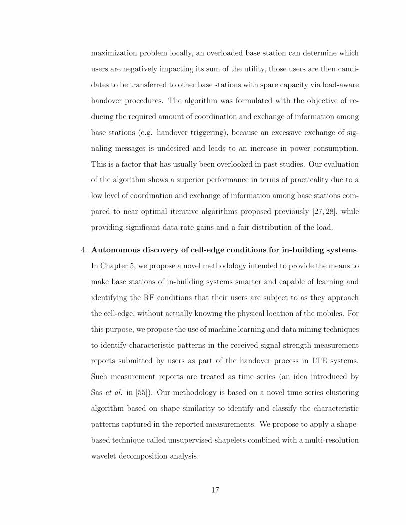
4. Autonomous discovery of cell-edge conditions for in-building systems.

In Chapter 5, we propose a novel methodology intended to provide the means to

make base stations of in-building systems smarter and capable of learning and

identifying the RF conditions that their users are subject to as they approach

the cell-edge, without actually knowing the physical location of the mobiles. For

this purpose, we propose the use of machine learning and data mining techniques

to identify characteristic patterns in the received signal strength measurement

reports submitted by users as part of the handover process in LTE systems.

Such measurement reports are treated as time series (an idea introduced by

Sas et al. in [55]). Our methodology is based on a novel time series clustering

algorithm based on shape similarity to identify and classify the characteristic

patterns captured in the reported measurements. We propose to apply a shape-

based technique called unsupervised-shapelets combined with a multi-resolution

wavelet decomposition analysis.

17

5. Optimization of handover parameters for in-building systems. In

Chapter 6 we propose a novel methodology to optimize handover parameters

for in-building systems. The objective of this methodology is to reduce han-

dover failures and the triggering of unnecessary handovers, and maximize the

QoS provided to users approaching the cell-edge. Our intention in this chapter

is to explore the development of a methodology that would allow base stations

to customize handover parameters at the user level in order to provide an op-

timal service. The key insight behind this methodology is the adjustment of

handover parameters based on the knowledge that base stations are able to

acquire regarding the RF conditions of their cell-edge. Such knowledge is ob-

tained through the application of the clustering algorithm described in chapter

5. Additionally, our methodology can also be considered as a load balancing

approach for users in “connected mode” (i.e. users actively exchanging data

with the base station). This is due to the fact that the optimization strategy

not only takes into consideration the levels of interference at the cell-edge but

also the loading conditions of the serving and target cell. The handover param-

eters are then adjusted accordingly in order to provide the highest quality of

service possible. To the best of our knowledge, a similar methodology for the

optimization of handover parameters has not been proposed in the literature.

1.4 Organization of the thesis

The contributions of this thesis are described in Chapter 2 through Chapter 6.

In Chapter 2 the tuning of site-specific path loss propagation models is described.

Chapter 3 provides a description of our system level simulator that includes a mo-

bility and traffic model, this tool can be considered as a walk/speed test simulator.

In Chapter 4 we discuss the load balancing issue in HetNets and provide the details

18

and evaluation of our proposed algorithm. Our methodology to provide base stations

of in-building systems with a mean to autonomously discover their cell-edge condi-

tions is described in Chapter 5. In Chapter 6, we describe our methodology to

optimize handover parameters for in-building systems. Finally, the thesis concludes

with an overall summary and a description of future research directions in Chapter

7.

Some of the chapters in this thesis contain sections quoted verbatim from five

publications by the author [24, 56–59]. Chapter 2 is based on the publications in

[24,56]. Chapter 3 is based on reference [59]. Chapter 4 is based on the publications

in [57,58]. Furthermore, chapters 5 and 6 are based on the manuscripts in [60] and [61]

respectively, these manuscripts are currently under review. All these publications and

manuscripts where co-authored with Dr. Raman Paranjape (second author).

Additionally, some portions of these papers have also been incorporated into this

introductory chapter.

19

Chapter 2

Local tuning of a site-specificpropagation path loss model for

microcell environments

New local and semi-global tuning methods for a 3D site-specific propagation path

loss model based on the UTD are proposed in this chapter. The purpose of the

tuning methods is to efficiently incorporate measured data in the prediction process to

enhance the accuracy of the path loss model in outdoor microcell environments. The

performance of the proposed tuning procedures is compared with a third method that

corresponds to a global tuning approach based on the Least Squares Error technique.

Our results show that the local tuning procedure outperforms any of the other tuning

methods by providing up to 35% reduction of the mean absolute error.

2.1 Introduction

In order to keep up with the exponential growth of the demand for mobile com-

munication services, network operators have been forced to increase the capacity of

their systems. Installation of new and smaller cell sites is a common approach to

increase the capacity of mobile systems like LTE networks. In such process, the use

of RF propagation prediction tools is essential. Propagation models play a vital role

during the design stage of new cell site deployments, several aspects related to the

performance of the network can be predicted based on the estimations provided by

propagation models.

RF propagation models have been extensively studied since the late 60’s. Ini-

20

tially, empirical models were developed to predict path losses in large macrocells

environments with many kilometers of coverage [9–11]. One of the most widely used

empirical models is the one proposed by Okumura and Hata [9]. The general equation

to calculate the path loss LdB is:

LdB = A + B log10 R (2.1)

Where A and B are functions of variables like the height of the transmitter, the

carrier frequency and the type of environment (medium-small city, large city, subur-

ban area, open area, etc.) and R is the distance between transmitter and receiver.

In general, empirical models provide the mean path loss based on simple equations

obtained empirically, like (2.1).

However, nowadays mobile network designers are focusing on the deployment of

smaller cell sites, like microcells, with coverage of a few blocks at most. As it was

stated in Sect. 1.2.1, the accuracy of empirical models in microcell environments is

poor, mostly because empirical models only take into account the propagation along

the direct path between transmitter and receiver. This means that only a single

propagation path is considered to estimate the propagation loss, hence ignoring an

essential phenomena in the propagation of radio frequency signals: the multipath ef-

fect. Furthermore, empirical models do not consider specific and detailed information

about the environment (e.g. topography of terrain, location and shape of buildings,

vegetation). Therefore, more accurate prediction models, e.g. site-specific models,

are more suitable for path loss prediction in small cell sites. These models are also

called deterministic models and are based on concepts of electromagnetic wave theory,

geometrical optics or on the UTD.

Ray tracing models, initially developed in the mid-90s, have become the most

widely used site-specific models nowadays [62,63]. Their popularity is due to the fact

that they can provide reasonably accurate results when sufficiently detailed infor-

21

mation of the physical environment is available. Using such detailed information, a

digital representation of the environment is generated. Electromagnetic wave theory

principles are then applied to predict the propagation losses. Their main disadvantage

is their complexity. They can be computationally expensive when applied to complex

outdoor environments. Significant work has been done in recent years to reduce the

processing times of ray tracing algorithms [64–67], however their implementation is

still cumbersome.

The main advantage of site-specific models is the fact that they provide a direct

modeling of the multipath phenomena occurring between transmitter and receiver

due to the presence of obstacles between them. Unfortunately, prediction errors occur

due to uncertainties in the digitized model of the physical environment, e.g. detailed

information about the electrical properties of building materials, the actual shape

and roughness of walls, location of windows and, the presence of relevant obstacles

like vegetation are usually difficult to determine [12].

Prediction errors on path loss estimations can greatly affect the design of a mobile

cellular system by providing poor coverage estimations. This situation can mislead

network operators to place base stations in locations that will not provide the desired

coverage. Therefore, it is common for RF engineers to perform drive and walk tests to

collect measurement data. Such measurements are then used to assess the coverage

during the design stage of a new deployment.

In this chapter, we investigate an effective procedure to enhance the accuracy of

site-specific path loss estimations by carefully integrating information from measured

data, collected during walk tests, in the prediction model. This process is known

as tuning of the model. It essentially adjusts the prediction model to the actual

conditions of the physical environment based on information from measured data.

Many approaches to tune propagation models have been proposed [13–24]. They

usually consist of the calculation of a unique set of optimal model parameters that

22

minimizes the disagreement between estimations and measurements, then the opti-

mized model is applied all over the entire target area. We consider these approaches

as global tuning procedures. Their main objective is to reduce the overall average

prediction error, even though the tuned model might actually increase the error in

certain areas of the map [24]. They have the disadvantage that such optimal set of

parameters is applied everywhere in the target area. Therefore, these global tuning

procedures are not able to correct prediction errors due to local causes, e.g. localized

mismatches between the digital model of the environment and the actual physical

environment.

In this chapter, we propose two novel tuning procedures for a site-specific path

loss prediction model: a semi-global and a local tuning. The propagation model

considered in this study is similar to the one we proposed in [24], this model consid-

ers four propagation mechanisms: free space, over-rooftop diffractions, vertical-edge

diffractions and single reflections. Our results show that our local tuning procedure

outperformed any of the other tuning methods considered in this study by providing

the lowest mean absolute error for any of our test transmitter locations. Tuning the

model locally provided a significant reduction of the mean absolute error between

measurements and predictions, the average reduction in the error was close to 35%

compared to the mean absolute error obtained with the untuned model.

The chapter is organized as follows: in Section 2.2 we provide a description of the

current tuning procedures for site-specific models. In Section 2.3 we provide details

about the propagation model used in this study. The proposed semi-global as well as

the local tuning procedures are described in Section 2.4. In Section 2.5 we provide

details about our measurement activity. Our results and discussion are presented in

Section 2.6. Finally we provide a summary in Section 2.7.

23

2.2 Related work

Tuning of site-specific models is not a trivial task. Many of these models are based

on theoretical principles. Therefore, to efficiently tune these models it is important

to identify the sources of prediction errors to be corrected by the tuning procedure.

Different tuning approaches have been proposed based on the error source. In [13],

a ray tracing model based on UTD is modified in order to include an adjustable pa-

rameter to account for the fact that the real impedance of walls is usually unknown;

using physical measurements a suitable value for this parameter can be found and

is applied to all the walls in the target area. In [14, 15] a similar prediction model

is tuned by finding an optimal value for the permittivity and conductivity of con-

crete walls. These approaches have the disadvantage that the dependency of UTD

diffraction/reflection coefficient equations on the electrical properties of materials is

non-linear and optimization is difficult; therefore, artificial intelligent techniques are

usually applied to obtain the optimal value of the parameters [15]. Furthermore, the

sensitivity of the models to these parameters is very low [68]; thus, applying compli-

cated algorithms to find optimal values of electrical properties of materials does not

provide significant improvements in the accuracy of the path loss estimations.

Other approaches consist of tuning propagation models to reduce prediction er-

rors caused by assumptions that over-simplify the digital representation of the en-

vironment. In [16–18], models like Bertoni-Walfish and Walfish-Ikegami, have been

modified to include adjustable parameters that account for inaccuracies caused by

simplifications like uniform separation and height of buildings. Those assumptions

usually do not match real conditions in all urban environments where buildings might

have very different shapes, orientations and separation between them. These ap-

proaches find optimal parameters values by applying techniques like Least Squares

Error (LSE) [16,19].

24

In [20–23], a probabilistic approach is proposed to reduce the uncertainty due to

unknown characteristics of obstacles in the environment. In [20–22], authors suggest

the use of random variables to model parameters like the average separation of build-

ings, orientation of roads, width of roads, and average heights of buildings; instead

of assuming a predefined constant value for each of those parameters. The tuning

procedure calculates the parameters of the probability distribution functions of the

random variables such that the prediction error is reduced. Similarly, in [23] a ray

tracing model is tuned by modeling the angle of reflections as a random variable.

This is done in order to account for the fact that the actual roughness of reflecting

surfaces is unknown; therefore the angle of incidence of a ray is not necessarily equal

to the angle of reflection as it is assumed in many models. Simple techniques like

LSE [21, 22] have been applied to find optimal parameters of the distribution func-

tions but more complicated methods like Particle Swarm Optimization (PSO) have

also been applied [20]. The mean error for these tuning methods has been reported

to be close to -2 dB.

The tuning approaches discussed so far are based on the calculation of a single

set of optimal parameters that are applied everywhere in the target area. Therefore,

these global tuning procedures are not able to correct prediction errors due to local

causes as it was mentioned before. Consider for example a digital representation of

the environment, that assumes that all buildings are box-shaped and all rooftops are

flat, local prediction errors are likely to occur in areas where such assumptions are not

valid, and these errors cannot be corrected with a global tuning approach as it was

shown in [24]. Therefore, a local tuning of the model is preferred, where information

from physical measurements is integrated into the prediction model at a local scale

and consequently multiple sets of values for the model parameters are calculated.

In the next section, we provide a description of the site-specific model used in this

study.

25

2.3 Path loss prediction model

The path loss prediction model, used during the design stage of a new cellular de-

ployment, should be selected considering factors like: cell size, type of environment

(rural, urban, suburban), available information about terrain, buildings, roads, trees

and characteristics of the transmitter and receiver antenna. In the case of outdoor mi-

crocells, line-of-sight (LOS) conditions typically do not occur and propagation mech-

anisms like diffractions, reflections and scattering are essential. Furthermore, the

propagation in urban microcells is highly dependent upon the location and orienta-

tion of buildings. Due to these facts, site-specific models are the most suitable option

for this type of environment.

In this study, we applied a site-specific propagation prediction model similar to

the one we proposed in [24]. Our model is based on ray tracing principles and the

classical UTD initially proposed by Kouyoumjian and Pathak in [69].

In a multipath channel, the received signal is a combination of a set of attenuated

and phase shifted replicas (rays) of the transmitted signal. Each one of these rays

reach the receiver after being reflected, diffracted and scattered by different objects

in the environment. Based on UTD principles, the total electric field at the receiver’s

location can be computed as the vector sum of the received electric field of each ray

arriving at the receiver as [62, 70]:

~ERx =

m∑j=1

~E j (2.2)

Where m is the number of rays reaching the receiver and ~E j is the received field

of the jth ray. The amplitude and phase of ~E j depend on the propagation path from

transmitter to receiver followed by the ray. According to UTD, the received field at

an observation point S due to a reflection (or diffraction) occurring at a point Q, is

26

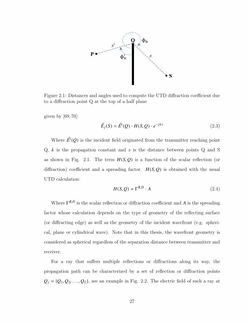
Figure 2.1: Distances and angles used to compute the UTD diffraction coefficient dueto a diffraction point Q at the top of a half plane

given by [69,70]:

~E j (S) = ~Ei (Q) · H (S,Q) · e− j ks (2.3)

Where ~Ei (Q) is the incident field originated from the transmitter reaching point

Q, k is the propagation constant and s is the distance between points Q and S

as shown in Fig. 2.1. The term H (S,Q) is a function of the scalar reflection (or

diffraction) coefficient and a spreading factor. H (S,Q) is obtained with the usual

UTD calculation:

H (S,Q) = ΓR,D · A (2.4)

Where ΓR,D is the scalar reflection or diffraction coefficient and A is the spreading

factor whose calculation depends on the type of geometry of the reflecting surface

(or diffracting edge) as well as the geometry of the incident wavefront (e.g. spheri-

cal, plane or cylindrical wave). Note that in this thesis, the wavefront geometry is

considered as spherical regardless of the separation distance between transmitter and

receiver.

For a ray that suffers multiple reflections or diffractions along its way, the

propagation path can be characterized by a set of reflection or diffraction points

Q j = {Q1,Q2, . . . ,QL}, see an example in Fig. 2.2. The electric field of such a ray at

27

Figure 2.2: Multiple half planes used to model buildings obstructing radial line be-tween point P and observation point S

an observation point S is given by [62,70]:

~E j (S) = ~Ei (Q1)L∏

l=1

ΓlR,D Ale jφ (2.5)

The incident field ~Ei (Q1) is typically calculated assuming LOS from the transmit-

ter location to the point Q1 as:

~Ei (Q1) = ~ET x ·e− j kr

r(2.6)

Where ~ET x is the transmitted electric field at a reference distance of one meter

from the transmitter and r is the distance between such reference distance and point

Q1.

Let W j denote the total field attenuation and phase shift suffered by the trans-

mitted field along the propagation path of the jth ray. Then, from (2.5) and (2.6),

W j can be calculated as:

W j =1

r

L∏l=1

ΓlR,D Al e− j kr j (2.7)

Where r j is the total length of the propagation path for the jth ray.

Using (2.7), (2.2) can be expressed in terms of the overall attenuation and phase

28

shift W as:

~ERx =

m∑j=1

~E j = W ~ET x (2.8)

With

W =m∑

j=1

W j (2.9)

For the calculation of the attenuation and phase shift of each ray W j , the prop-

agation model applied in this chapter considers four propagation mechanism: free

space propagation (LOS), over-rooftop diffractions, vertical-edge diffractions and re-

flections. Scattering losses due to foliage were also included. A detailed description

of the model is provided below.

2.3.1 Free space propagation

A ray is considered to propagate in LOS conditions if at least 55% of the first Fresnel

zone is clear of obstacles [71]. If such ray exists, then its contribution to the total

received electric field is calculated using (2.6).

2.3.2 Over-rooftop and vertical-edge diffractions

Over-rooftop diffractions are evaluated along the radial profile between transmitter

and receiver. Every building obstructing the radial profile is modeled as a perfectly

absorbing half plane perpendicular to the ground plane (multiple knife-edge model)

[72, 73]. The height of the half plane is equal to the height of the building. The

orientation of the edge of the half plane is assumed to be perpendicular to the radial

line joining the transmitter and receiver. The diffraction coefficient for the half plane

model assuming perpendicular incidence is given by [69,72,73]:

ΓnD (φn, φ

′n, Ln) =

−e jπ/4

2√

2πk cos(α/2)· F[kL cos2(α/2)] (2.10)

29

Where φn and φ′n are the angle of the diffracted and incident ray relative to the

nth half plane respectively, as shown in Fig. 2.1. And α is given by:

α = φn − φ′n (2.11)

Ln is a distance factor for the nth half plane, for spherical waves it is given by

[70,74]:

Ln =sn sn−1

sn + sn+1(2.12)

With the distances sn and sn−1 as shown in Fig. 2.2. The function F is called a

transition function and its calculation is based on the following Fresnel integral:

F (x) = 2 j√

xe j x∫ ∞

√x

e− ju2du (2.13)

For the case of diffraction due to multiple half planes, the spreading factor An due

to the nth half plane, is given by [74]:

An =

√√√ ∑n−1k=0 sk

sn ·(∑n−1

k=0 sk + sn) (2.14)

The diffraction coefficient ΓDn and spreading factor An are calculated for every

building that significantly contributes to the diffraction loss, i.e. each building whose

half plane model is touched by an imaginary rubber band stretched over the radial

profile from transmitter to receiver. The imaginary rubber band and diffraction points

due to multiple half planes are shown in Fig. 2.2.

Vertical-edge diffractions are evaluated similarly as over-rooftop diffractions. Cor-

ners of buildings obstructing the radial line between transmitter and receiver are

modeled as half planes. The procedure applied for over-rooftop diffractions is then

followed.

30

2.3.3 Reflections

The specular reflection coefficient ΓR can be computed as shown in (2.15), assuming

vertical polarization of the transmitter antenna [71]:

ΓR =−εr sin θinc +

√εr − cos2 θinc

εr sin θinc +√εr − cos2 θinc

(2.15)

Where θinc is the angle between the incident ray and the perpendicular to the

reflecting surface and εr is the relative permittivity of the reflecting surface.

Our model automatically inspect the area surrounding the transmitter and receiver

in order to determine the existence of obstacles, like walls, that can be sources of

reflected rays. For simplicity, all walls are assumed to be flat, smooth and made up of

concrete. Their relative permittivity was fixed at the typical value of 7, as proposed

in [70].

2.3.4 Scattering losses due to foliage

The received signal is also affected by other obstructions like trees, street signs and

light poles. They provide additional attenuation to the RF signal that can be quan-

tified as scattering losses. In our model, we consider scattering losses due to the

presence of deciduous trees obstructing the propagation path. These losses are com-

puted according to the model proposed by Benzair [75]. According to this model,

when the receiver is located in the shadow of one or more trees, the scattering losses

can be approximated by:

Lscatt (dB) = d f · a · f b[GHz] (2.16)

Where d f is the depth of foliage, a and b are factors that depend on the season:

in the summer a = 0.57, b = 0.6; in the winter a = 0.36, b = 0.43.

Scattering losses are included in the loss of each ray if the corresponding propa-

31

gation path goes through an area covered by trees.

2.3.5 Propagation path loss

The propagation path loss is defined as:

L =PRx

PT x(2.17)

Where PRx and PT x are the received and transmitted power respectively. The

received power PRx is calculated as [70,71]:

PRx = Ae f f

���~ERx���2

ηo(2.18)

Where Ae f f is the effective aperture of the antenna and ηo is the intrinsic

impedance of free space. For omni-directional antennas 1, Ae f f = λ2/4π as described

in [71]. Therefore, the corresponding transmitted power PT x is calculated as:

PT x =4π

ηo

���~ET x���2

(2.19)

Hence, using (2.8) and (2.17) to (2.19), the total propagation loss can be expressed

in terms of the total attenuation and phase shift W as [70]:

L = *.,

λ

4π

���~ERx���

���~ET x���

+/-

2

=

(λ

4π|W |

)2(2.20)

1Note that for path loss prediction, we assume the use of ideal omni-directional antennas. Inpractice, the gains of the antennas have to be included if link budget calculations are applied toestimate received signal power (see (2.30))

32

Or in dB units, we have:

LdB = 20 log10

(λ

4π|W |

)(2.21)

2.3.6 Model parameters

In order to tune the propagation model, a set of adjustable parameters is introduced

in our model calculations. The value of such parameters will be defined by the tuning

algorithm. For simplicity, we have classified the rays reaching a specific receiver’s

location in 5 categories according to their main propagation mechanism, i.e. free

space ray, over-roof top diffracted ray, vertical-edge diffracted rays and reflected rays.

Contributions to the received signal due to rays suffering combinations of multiple

diffractions and reflections are not considered. Based on this classification and using

(2.9), the total attenuation and phase shift W between the transmitter and a particular

receiver’s location can be expressed as:

W = WFS +WRD +WV D +WR (2.22)

Where:

• WFS total attenuation and phase shift of free space ray.

• WRD total attenuation and phase shift of over-rooftop diffracted ray.

• WV D total combined attenuation and phase shift of all rays reaching the receiver

due to vertical-edge diffractions only.

• WR total combined attenuation and phase shift of all rays reaching the receiver

due to single reflections only.

33

With:

WV D =∑

j∈VD

W j WR =∑j∈R

W j (2.23)

Where VD and R are sets containing reflected and vertical-edge diffracted rays

reaching the receiver’s location, respectively.

At this point, we introduce the model parameter set M = {m1,m2,m3,m4,m5}.

Equation (2.22) is then modified to include these model parameters as:

W = m1WFS + m2WRD + m3WV D + m4WR + m5 (2.24)

The purpose of the tuning algorithm is to determine suitable values of the pa-

rameters in M such that the disagreement between physical measurements and the

model predictions is minimized. In general, parameters in M are complex-valued.

The formulation of (2.24) allows the tuning procedure to individually adjust each one

of the main propagation mechanism supported by our propagation model according

to the measured data. Parameter m5 is included in (2.24) to account for those ad-

ditional rays reaching the receiver through propagation paths not considered by the

propagation model, e.g. rays suffering combinations of diffractions and reflections.

2.4 Global, Semi-global and Local tuning

In this section three approaches to tune the propagation model are presented. The

global tuning procedure previously proposed in [24] is included in this chapter for

comparison purposes. Two new approaches are proposed: a semi-global and a local

tuning procedure. In the next subsections we provide more details about each one of

these approaches and a comparison analysis is provided in our results.

34

2.4.1 Global tuning based on LSE

The global tuning approach applied in this chapter is similar to the one proposed in

[24]. The measured values of path losses are compared with the estimations provided

by the prediction model. The LSE method is then applied to find optimal values of

the parameters inM such that the mean square error is minimized. Finally, the path

loss predictions are recalculated with (2.21) and (2.24) using the optimal values of

the model parameters in all receiver locations in the target area.

2.4.2 Semi-global tuning

One of the main disadvantages of the global tuning approach is the fact that only a

unique set of values for the model parameters is found and applied all over the entire

map. Therefore, prediction errors due to local errors or over-simplifications of the

model of the physical environment are not corrected properly. In order to improve

the tuning procedure, a semi-global and local tuning approaches are proposed in this

chapter. The semi-global tuning procedure consists of three basic steps:

First step: Receiver locations are classified in groups based on the level of obstruc-

tion of the propagation path to the transmitter. We determine the level of obstruction

of the path based on the number of buildings obstructing the direct path between

transmitter and receiver. Each group of receiver’s locations Gm is defined as:

Gm = {(x, y) ∈ G|m buildings block the direct path} (2.25)

Where (x, y) are the coordinates of a receiver’s location and G corresponds to the

target area. Based on (2.25), all those receiver locations with LOS conditions belong

to group Go. Similarly, all those receiver locations with one building obstructing the

direct path between transmitter and receiver belong to G1. In the same way, other

35

groups are created if there exist receiver locations with two obstructing buildings and

so forth. This classification of receiver locations based on the level of obstruction

of the propagation path is motivated by an observation made in our previous study

in [24]. We showed that the accuracy of the path loss predictions decrease as the

propagation path becomes more complex (e.g. high level of obstruction of the direct

path between receiver and transmitter) and therefore the value of the parameters

used to tune the prediction model should be adapted accordingly.

Second step: A set of optimal values of the model parameters are calculated for

each group of receiver locations Gm. Such optimal set of parameters is calculated

based only on measured data gathered in places belonging to that group of receiver

locations. Let Mm be the set of optimal parameters for group Gm. Measured data

used to calculate the values of the parameters Mm are selected according to (2.26):

Dm ={d j ∈ D|(x j, y j ) ∈ Gm

}(2.26)

Where D is the set containing all measured data and (x j, y j ) are the coordinates

of the place where measurement d j was collected. According to (2.26), only measured

data gathered in receiver locations belonging to Gm are used to calculate the values of

the set of parameters Mm. For example, optimal set of parameters Mo is computed

based only on measured data collected in locations belonging to Go. The set of

optimal parameters for each group Gm is calculated using the LSE method.

Third step: The path loss predictions are recalculated with (2.21) and (2.24) using

the set of optimal parameters that corresponds to the group where the receiver is

located.

This approach has the advantage that the tuning procedure can correct errors at a

particular receiver location considering only measurements that were taken in places

with similar levels of obstruction of the path. The approach is considered a semi-

36

global tuning method, in the sense that measurements used to calculate the optimal

parameters for each group Gm could have been collected anywhere in the target area

G; not necessarily close to the location where the tuning is to be applied.

2.4.3 Local tuning

As we have mentioned before, the most significant source of prediction errors is due

to inaccurate modeling of the physical environment. Furthermore, there is a trade-off

between complexity of the model and accuracy. In many instances, assumptions and

simplifications are applied to prediction models in order to reduce their complexity.

This is done to facilitate their application in complicated outdoor environments. The

price paid is a reduction in the accuracy.

The insight behind the local tuning procedure is to adjust the model parameters

at a local scale. Consider a particular receiver’s location. The diffractions, reflections

and scattering suffered by the transmitted signal are directly affected by the obstacles

around that receiver’s location, especially buildings. If the size and shape of buildings

around that location are erroneously described in the model of the physical environ-

ment (e.g. due to lack of information), then it is expected that such inaccuracies will

affect the quality of the prediction.

Therefore, a local tuning procedure should be able to identify measured data

that captures the actual propagation conditions around a specific receiver’s locations.

Such information should then be applied to determine a suitable value of the model

parameters for that receiver’s location. This is a significant difference with respect

to the global tuning procedure that calculates a unique set of values of the model

parameters based on measured data collected anywhere in the map, in places subject

to a diverse variety of propagation path characteristics. Our local tuning procedure

can be thought of as a refinement of the semi-global tuning, three basic steps can be

37

used to describe this tuning approach:

First step: Consider a receiver located at a point with coordinates (xi, yi). The

first step of the local tuning consists of identifying a set of measurements Di gathered

at locations in the vicinity of the point (xi, yi), e.g. by defining a circular region of

radius R centered in (xi, yi) and identifying all measured data gathered inside such

region, i.e.:

Di ={d j ∈ D |

(xi, yi) − (x j, y j ) < R

}(2.27)

Based on our previous experimental observations for an urban environment, a

value of R = 20m provides reasonably accurate results [24].

Second step: Measurements in Di that were taken in places whose propagation

characteristics are similar to the ones in (xi, yi) are selected. This is done by creating

a subset of Di, that we denote by D∗i , containing measurements collected at places

where the dominant propagation mechanism matches the one at the receiver’s location

(xi, yi). The subset D∗i is given by:

D∗i ={d j ∈ Di |B( j) = B(i)

}(2.28)

Where B(i) corresponds to the dominant propagation mechanisms at point (xi, yi).

B(i) can be any of the propagation mechanisms supported by the prediction model:

FS, RD, VD or R as described in Section 2.3. The dominant propagation mechanism

at point (xi, yi) is given by:

WB(i) = max{|WFS(i) |, |WRD(i) |, |WV D(i) |, |WR(i) |

}(2.29)

Third step: Measurements in D∗i are used to calculate an optimal set of values of

the model parameters Mi by applying LSE. Such set of parameters values are then

used to calculate the tuned path loss value at point (xi, yi).

38

These three steps of the local tuning procedure are repeated for every location of

the receiver where the tuning is to be applied.

In cases where it is not possible to identify enough measurements to calculateMi,

then the semi-global tuning procedure is applied to tune the model.

Based on the three steps described before, it is clear that multiple sets of model

parameters are calculated by our local tuning procedure, where each set of parameters

is used to adjust the model based on information of the local propagation conditions

captured by the measured data.

2.4.3.1 Practical considerations

From a practical point of view, it is important for network operators to minimize the

time and resources spent collecting walk and drive test data. As we mentioned before,

we have shown in [24] that the accuracy of the path loss predictions decrease as the

propagation path becomes more complex. This observation can then be applied to

make the collection of measured data more efficient. Essentially, this means that data

collection efforts should be concentrated in gathering measurements in areas where it

is expected that the prediction model will be inaccurate.

Our local tuning procedure, combined with the semi-global tuning approach, are

aimed at taking advantage of a limited set of measured data gathered specifically at

those strategic locations where the tuning of the model is most needed.

The performance of each of the three tuning procedures discussed in this section was

evaluated using experimental data. The details about the measurement equipment

as well as the procedure to gather the data are described in the next section.

39

Table 2.1: Selected test locations for test transmitter

Location # BuildingTransmitterheight (m)

1 South Tower Residences 372 Dr. John Archer Library 283 Education 214 Riddell Centre 145 Research & Innovation Centre 23

2.5 Gathering of experimental data

A signal strength measurement activity was carried out during the summer time in

the main campus of the University of Regina in Saskatchewan, Canada. Our test

transmitter was placed at five different locations on campus and an average of 630

measurements were recorded for every test location. The test transmitter and receiver

are equipped with calibrated CC2530 transceiver modules, manufactured by Texas

Instruments. Additional amplifiers were implemented to reach the desired transmit

power of 26 dBm.

Measurements were taken at 2.480 GHz with a channel bandwidth of 5 MHz. Ver-

tically polarized dipole antennas were used in the transmitter and receiver units, both

antennas with 5 dBi of gain. The five locations selected to place the test transmitter

correspond to the rooftop of five buildings on campus as indicated in Fig. 2.3. The

height of the transmitter for each one of these locations is provided in table 2.1.

Each of the five measurement sessions consisted of a walk test on the sidewalks

and roads around campus. The height of the receiving antenna was 1.5 meters above

ground level.

Our test signal consisted of bursts of 100 packets of data sent continuously by the

transmitter. Each packet with approximately 60 bytes of information transmitted at

250 Kbps following the IEEE802.15.4 protocol. Every signal strength measurement

40

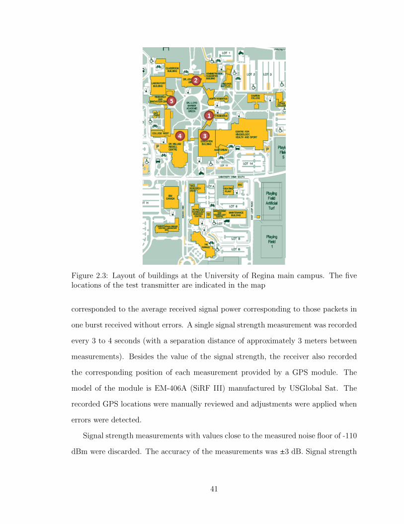
Figure 2.3: Layout of buildings at the University of Regina main campus. The fivelocations of the test transmitter are indicated in the map

corresponded to the average received signal power corresponding to those packets in

one burst received without errors. A single signal strength measurement was recorded

every 3 to 4 seconds (with a separation distance of approximately 3 meters between

measurements). Besides the value of the signal strength, the receiver also recorded

the corresponding position of each measurement provided by a GPS module. The

model of the module is EM-406A (SiRF III) manufactured by USGlobal Sat. The

recorded GPS locations were manually reviewed and adjustments were applied when

errors were detected.

Signal strength measurements with values close to the measured noise floor of -110

dBm were discarded. The accuracy of the measurements was ±3 dB. Signal strength

41

measurements were converted to path loss values using (2.30).

Path loss = PT x + GT x + GRx − Signal strength (2.30)

Where PT x corresponds to the transmission power, GT x and GRx correspond to

the antenna gain of transmitter and receiver units respectively.

The environment of the University of Regina campus can be classified as urban

with flat terrain and irregular location, size and orientation of buildings. The average

building elevation is 17 m with a total of 27 buildings. The area covered by this study

has a rectangular shape with dimensions 600 m by 1000 m as shown in Fig. 2.3.

2.6 Results & Discussion

We performed extensive signal strength measurements as described in Section 2.5

for each one of the five locations of the test transmitter. Our signal strength mea-

surements were converted to path loss values using (2.30). The resulting path loss

measurements were compared with the estimations provided by the propagation pre-

diction model described in Section 2.3. The propagation model was tuned with each

one of the tuning procedures described in Section 2.4: global, semi-global and local.

In the following subsections, we describe our results.

2.6.1 Evaluating the accuracy of the tuned model

For each run of our experiment, the set of measurements collected for each location

of the transmitter was randomly divided in two subsets. The first half of the mea-

surements were used to tune the model (globally, semi-globally and locally), we call

this subset of measurements the training set. The second half of measurements were

used to evaluate the performance of each one of the tuning procedures, we call this

42

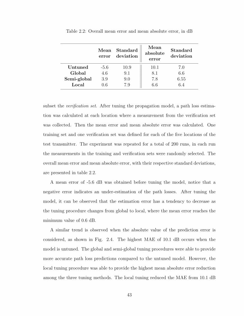
Table 2.2: Overall mean error and mean absolute error, in dB

Meanerror

Standarddeviation

Meanabsolute

error

Standarddeviation

Untuned -5.6 10.9 10.1 7.0Global 4.6 9.1 8.1 6.6

Semi-global 3.9 9.0 7.8 6.55Local 0.6 7.9 6.6 6.4

subset the verification set. After tuning the propagation model, a path loss estima-

tion was calculated at each location where a measurement from the verification set

was collected. Then the mean error and mean absolute error was calculated. One

training set and one verification set was defined for each of the five locations of the

test transmitter. The experiment was repeated for a total of 200 runs, in each run

the measurements in the training and verification sets were randomly selected. The

overall mean error and mean absolute error, with their respective standard deviations,

are presented in table 2.2.

A mean error of -5.6 dB was obtained before tuning the model, notice that a

negative error indicates an under-estimation of the path losses. After tuning the

model, it can be observed that the estimation error has a tendency to decrease as

the tuning procedure changes from global to local, where the mean error reaches the

minimum value of 0.6 dB.

A similar trend is observed when the absolute value of the prediction error is

considered, as shown in Fig. 2.4. The highest MAE of 10.1 dB occurs when the

model is untuned. The global and semi-global tuning procedures were able to provide

more accurate path loss predictions compared to the untuned model. However, the

local tuning procedure was able to provide the highest mean absolute error reduction

among the three tuning methods. The local tuning reduced the MAE from 10.1 dB

43

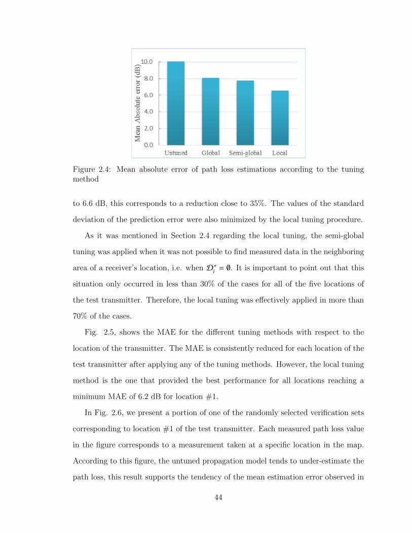
Figure 2.4: Mean absolute error of path loss estimations according to the tuningmethod

to 6.6 dB, this corresponds to a reduction close to 35%. The values of the standard

deviation of the prediction error were also minimized by the local tuning procedure.

As it was mentioned in Section 2.4 regarding the local tuning, the semi-global

tuning was applied when it was not possible to find measured data in the neighboring

area of a receiver’s location, i.e. when D∗i = ∅. It is important to point out that this

situation only occurred in less than 30% of the cases for all of the five locations of

the test transmitter. Therefore, the local tuning was effectively applied in more than

70% of the cases.

Fig. 2.5, shows the MAE for the different tuning methods with respect to the

location of the transmitter. The MAE is consistently reduced for each location of the

test transmitter after applying any of the tuning methods. However, the local tuning

method is the one that provided the best performance for all locations reaching a

minimum MAE of 6.2 dB for location #1.

In Fig. 2.6, we present a portion of one of the randomly selected verification sets

corresponding to location #1 of the test transmitter. Each measured path loss value

in the figure corresponds to a measurement taken at a specific location in the map.

According to this figure, the untuned propagation model tends to under-estimate the

path loss, this result supports the tendency of the mean estimation error observed in

44

Figure 2.5: Mean absolute error per location of the transmitter for different tuningmethods

Figure 2.6: Example of path loss values for location #1 of the test transmitter.Measured path loss values as well as the corresponding untuned and tuned estimationsare presented

table 2.2, where the untuned model provided a negative mean error. Furthermore,

the locally tuned estimations provided the most accurate results compared to the

measured path loss values. The random nature of the path loss values in this figure

is due to the procedure followed to select the verification set and training set for each

location of the test transmitter, such sets were randomly selected for each run of the

experiment.

45

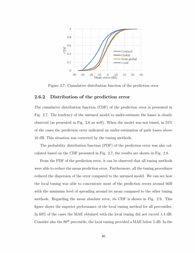
Figure 2.7: Cumulative distribution function of the prediction error

2.6.2 Distribution of the prediction error

The cumulative distribution function (CDF) of the prediction error is presented in

Fig. 2.7. The tendency of the untuned model to under-estimate the losses is clearly

observed (as presented in Fig. 2.6 as well). When the model was not tuned, in 55%

of the cases the prediction error indicated an under-estimation of path losses above

10 dB. This situation was corrected by the tuning methods.

The probability distribution function (PDF) of the prediction error was also cal-

culated based on the CDF presented in Fig. 2.7, the results are shown in Fig. 2.8.

From the PDF of the prediction error, it can be observed that all tuning methods

were able to reduce the mean prediction error. Furthermore, all the tuning procedures

reduced the dispersion of the error compared to the untuned model. We can see how

the local tuning was able to concentrate most of the prediction errors around 0dB

with the minimum level of spreading around its mean compared to the other tuning

methods. Regarding the mean absolute error, its CDF is shown in Fig. 2.9. This

figure shows the superior performance of the local tuning method for all percentiles.

In 60% of the cases the MAE obtained with the local tuning did not exceed 1.4 dB.

Consider also the 80th percentile, the local tuning provided a MAE below 5 dB. In the

46

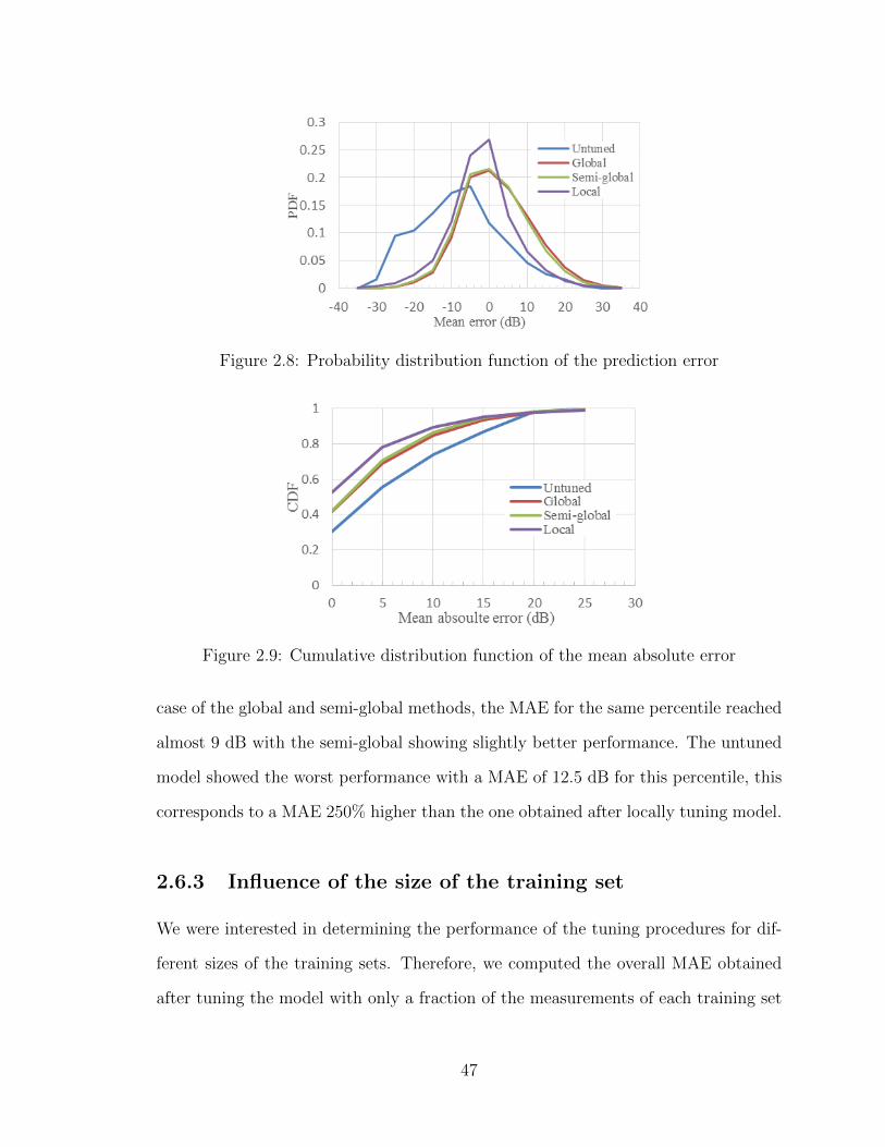
Figure 2.8: Probability distribution function of the prediction error

Figure 2.9: Cumulative distribution function of the mean absolute error

case of the global and semi-global methods, the MAE for the same percentile reached

almost 9 dB with the semi-global showing slightly better performance. The untuned

model showed the worst performance with a MAE of 12.5 dB for this percentile, this

corresponds to a MAE 250% higher than the one obtained after locally tuning model.

2.6.3 Influence of the size of the training set

We were interested in determining the performance of the tuning procedures for dif-

ferent sizes of the training sets. Therefore, we computed the overall MAE obtained

after tuning the model with only a fraction of the measurements of each training set

47

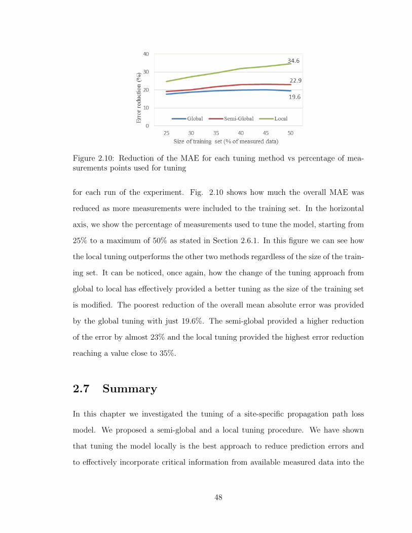
Figure 2.10: Reduction of the MAE for each tuning method vs percentage of mea-surements points used for tuning

for each run of the experiment. Fig. 2.10 shows how much the overall MAE was

reduced as more measurements were included to the training set. In the horizontal

axis, we show the percentage of measurements used to tune the model, starting from

25% to a maximum of 50% as stated in Section 2.6.1. In this figure we can see how

the local tuning outperforms the other two methods regardless of the size of the train-

ing set. It can be noticed, once again, how the change of the tuning approach from

global to local has effectively provided a better tuning as the size of the training set

is modified. The poorest reduction of the overall mean absolute error was provided

by the global tuning with just 19.6%. The semi-global provided a higher reduction

of the error by almost 23% and the local tuning provided the highest error reduction

reaching a value close to 35%.

2.7 Summary

In this chapter we investigated the tuning of a site-specific propagation path loss

model. We proposed a semi-global and a local tuning procedure. We have shown

that tuning the model locally is the best approach to reduce prediction errors and

to effectively incorporate critical information from available measured data into the

48

propagation path loss prediction process. According to our results, tuning the model

locally provides a significant reduction of the mean absolute error between measure-

ments and estimations, such reduction is close to 35% compared to the case when the

model is not tuned. Furthermore, according to the CDF of the MAE, for the 80th

percentile of our observations, the local tuning provided a substantial reduction of the

mean absolute error, reaching up to 250% error reduction compared to the untuned

model for the same percentile. The local tuning procedure outperformed the global

and semi-global tuning methods for any percentile, for any size of the training set and

for any location of the test transmitter. Our results have shown that a local tuning

of the path loss prediction model provides a flexible way to optimize the parameters

of the propagation model, since prediction errors are corrected based on very specific

local propagation conditions.

49

Chapter 3

Walk/Speed test simulator forcellular network planning

A walk test is a tedious and time consuming task for mobile network operators,

typically required to verify signal levels and quality of service provided by a newly

deployed cell site. The resources spent in such tests can be reduced with the use

of accurate planning and design tools. In this chapter, we describe and validate

an LTE/LTE-A downlink simulator that is capable of accurately modeling the main

performance metrics collected during walk tests. We evaluated the accuracy of the

simulator to model and capture the characteristic behavior of the quality and strength

of the received signal as users are handed over between cells. Furthermore, we evalu-

ated the capability of the walk test simulator to accurately predict the user experience

at the handover region (in terms of the downlink data rate) under different network

loading conditions. Two traffic models were tested: a Quality of Service (QoS) based

model and the typical Full Buffer model. Our validation was carried out based on

experimental walk test data collected from a live LTE network. Our results indicated

a significant reduction of the estimation error of the data rate of up to 86% with the

QoS-aware traffic model.

3.1 Introduction

The planning of LTE/LTE-A systems is an essential task for network operators. They

face important challenges, for example satisfying an ever growing demand for data

services and the deployment of new technologies like Voice over LTE (VoLTE). Addi-

50

tionally, there is a need to reduce costs during the design and planning stages as well

as to reduce the time spent in these tasks.

Simulation models are essential tools intended to guide the design and planning

process. There exist basic tools that provide RF estimations and basic calculations of

the Quality of Service (QoS) (e.g. maximum achievable data rate) that users would

receive. Commercially available tools like Mentum Planet [76] and iBwave [77] are

some examples of this type of software tools. Mentum Planet is applied in the design

and planning of outdoor systems (e.g. macrocells and microcells), whereas iBwave

is applied for in-building systems (e.g. Distributed Antenna Systems (DAS) and

picocells).

One of the most important tasks during the network planning stage is to make

sure the system is designed to provide the highest QoS possible in the target area.

One key factor to consider during network planning is user mobility and the QoS

provided to users as they move, particularly in high traffic areas, e.g. downtown

areas, university campus, shopping centres. In most cases, commercially available

tools have the limitation of modeling the spatial distribution of users in a static

fashion, hence ignoring the effects of user mobility patterns on network performance.

This is particularly important for the evaluation of the quality of service as users

move between coverage areas. Furthermore, such tools also have limited capabilities

to model the dynamic behaviour of actual data traffic in modern networks. Typically,

a Full Buffer model is assumed, i.e. all base stations have an infinite amount of data

to be delivered to each one of its connected users.

Additionally, many of the contributions described in the literature related to the

area of HetNets, have been evaluated also assuming a static distribution of users

and simplistic traffic models [25, 26]. Recently, there have been important efforts to

incorporate reliable user mobility and traffic models applicable to HetNets [30–32].

Due to this relative lack of simulation models for LTE/LTE-A systems capable of

51

accurately modeling user mobility and predicting the QoS for site-specific scenarios,

operators are usually forced to perform numerous walk and speed tests to verify the

actual user experience in different locations of the service area.

During a walk test, a technician carries a mobile device capable of collecting a set

of different physical measurements, for example the Reference Signal Received Power

(RSRP) and the Reference Signal Received Quality (RSRQ) values from the serving

cell, signal-to-noise-plus-interference ratio (SINR), downlink data rates of HTTP or

FTP transfers, data rates for video streaming and many other tests. The process

of the walk test is time consuming and tedious, since the collection of data usually

requires multiple walks all over the service area. Furthermore, after collecting the data

a significant amount of effort is dedicated to the post-processing of the information.

In this chapter we describe an LTE/LTE-A downlink simulator that incorporates

a model for user mobility. This software can be used by network operators to simulate

walk tests during the design and planning stages of the mobile network. Furthermore,

we incorporate a realistic traffic model based on Quality of Service requirements

defined according to the type of traffic that a specific user demands. We validated

our results with measurement data collected from actual walk tests and compared the

accuracy of our QoS-based traffic model with the popular Full Buffer traffic model.

The chapter is organized as follows: a brief overview of the research work in this

area is presented in Sect. 3.2. In Sect. 3.3 we provide a high level description of

the downlink simulator, including the mobility and traffic models. In Sect. 3.4 we

describe the collection of experimental data. Our results and analysis are presented

in Sect. 3.5 and finally we provide a summary in Sect. 3.6

52

3.2 Related work

Most traditional commercially available simulation tools, e.g. Mentum Planet and

iBwave, provide basic functionalities to estimate the achievable data rate that a spe-

cific user may receive based on factors like: the quality and strength of the received

signal. These simulation tools also allow the operators to manually create traffic

maps. These maps are used to describe the spatial distribution of the users in the

area of interest as well as their demand. These maps are based on demographic data

and estimations of the users demand. In most cases, the simulation tools provide

basic insights regarding the performance of the network under the assumption that

the users are static, hence ignoring the effects of user mobility.

Open source simulation tools, like the Vienna simulator [78, 79], provide the ca-

pability to simulate LTE networks. However, the propagation of signals (e.g. large

and small scale fading) is modeled according to statistical models, hence site-specific

results cannot be obtained. Additional modules would need to be implemented in

order to incorporate custom environment scenarios (e.g. a specific building layout)

in such simulation tools.

On the other hand, in many cases the contributions proposed in the research

literature have been assessed assuming a static distribution of users. Some examples

are the research works in [25, 26], where general analytical models of HetNets are

proposed assuming a uniform distribution of users and without considering any traffic

model. In [25], a theoretical model for the analysis of the downlink of a multi-tier

HetNet was proposed. Based on the random spatial model proposed in [80] (a Poisson

Point Process is used to model the location of base stations of each tier), the authors

developed an analytical model to quantify the probability distribution of the SINR

as well as the outage probability in terms of the base station density for each tier.

A similar analytical model was described in [26]. However, in these approaches the

53

quality of service provided to users is not included in the formulation of the model

and neither a traffic nor a user demand model is provided. In some other instances,

user demand has been modeled according to the traditional full buffer model (i.e. all

base stations have an infinite amount of data to deliver to each one of their users),

but also assuming users are static [27–29].

In modern mobile networks, traffic demand is segmented according to the type

of applications and services that mobiles are executing. For example, a portion of

the users are running bandwidth-intensive applications, while another portion of the

users are performing light browsing and file transfer activities, and another portion

of the traffic could be due to non-user initiated connections (like automatic update of

smartphone “apps”). This segmentation of the traffic is also subject to change during

the day and it is in general not captured by the full buffer traffic model. The need

to develop traffic and mobility models that emulate the actual behavior of users has

been recognized in recent years in [30–32].

In [30], dynamic traffic is included in system simulations, initiation of downlink

data sessions are modeled as a random Poisson process assuming all users are de-

manding files with the same size. According to their model, the time between new

data sessions is exponentially distributed. In [31], a density map is used to randomly

place users in the service area and the popular full buffer traffic model is then applied.

Finally, in [32], the authors identified that proper mobile network modeling should

include a dynamic user population in terms of traffic demand. Most of the current

research on HetNets has focused on static steady state formulations, e.g. the full

buffer traffic model. And such formulations do not capture realistic load variations

with time and space. Therefore, they provide substantially different performance

characteristics compared to actual networks.

In this chapter, we describe an LTE/LTE-A downlink simulator capable of model-

ing the walk/speed tests carried out by network operators during the planning stage

54

of a new cell site. With the advantage that this simulation tool incorporates a realistic

traffic model based on QoS requirements, such requirements are defined according to

the type of traffic that a specific user demands, this is an approach not considered

in [30–32]. With this simulation tool, we quantify the effects of the traffic model on

the accuracy of the data rate estimations, this aspect was not included in the general

analytical models in [25, 26]. The simulator was validated with measurement data

collected from a live LTE network, with emphasis on cell-edge regions. This is due

to the fact that at the cell-edge the QoS tend to degrade, and it is fundamental for a

new deployment to guarantee acceptable QoS and continuity of service in such areas.

Our simulator was capable of providing high accurate modeling of the walk/speed

tests process when our traffic model was applied as opposed to the traditional full

buffer model.

3.3 LTE/LTE-A Downlink Simulator

In this chapter we are interested in modeling user mobility and estimating the user

experience provided to mobile users as they move, we quantify the user experience in

terms of the downlink data rate. Our analysis focuses on the evaluation of the effects

of different factors on the user experience, e.g. user’s traffic demand, load levels of

the network, quality of the received signal and user mobility.

Mobile network simulators can be classified in two main categories [79]: link level

simulators and system level simulators. Link level simulators are intended to provide

models for channel estimation, channel encoding, adaptive modulation and coding

(AMC), inter-cell interference cancellation techniques and many other factors related

to physical-layer modeling. On the other hand, system level simulators focus on higher

level issues related to the network operation, e.g. radio resource sharing, scheduling al-

gorithms, mobility management, interference management, self-organizing functional-

55

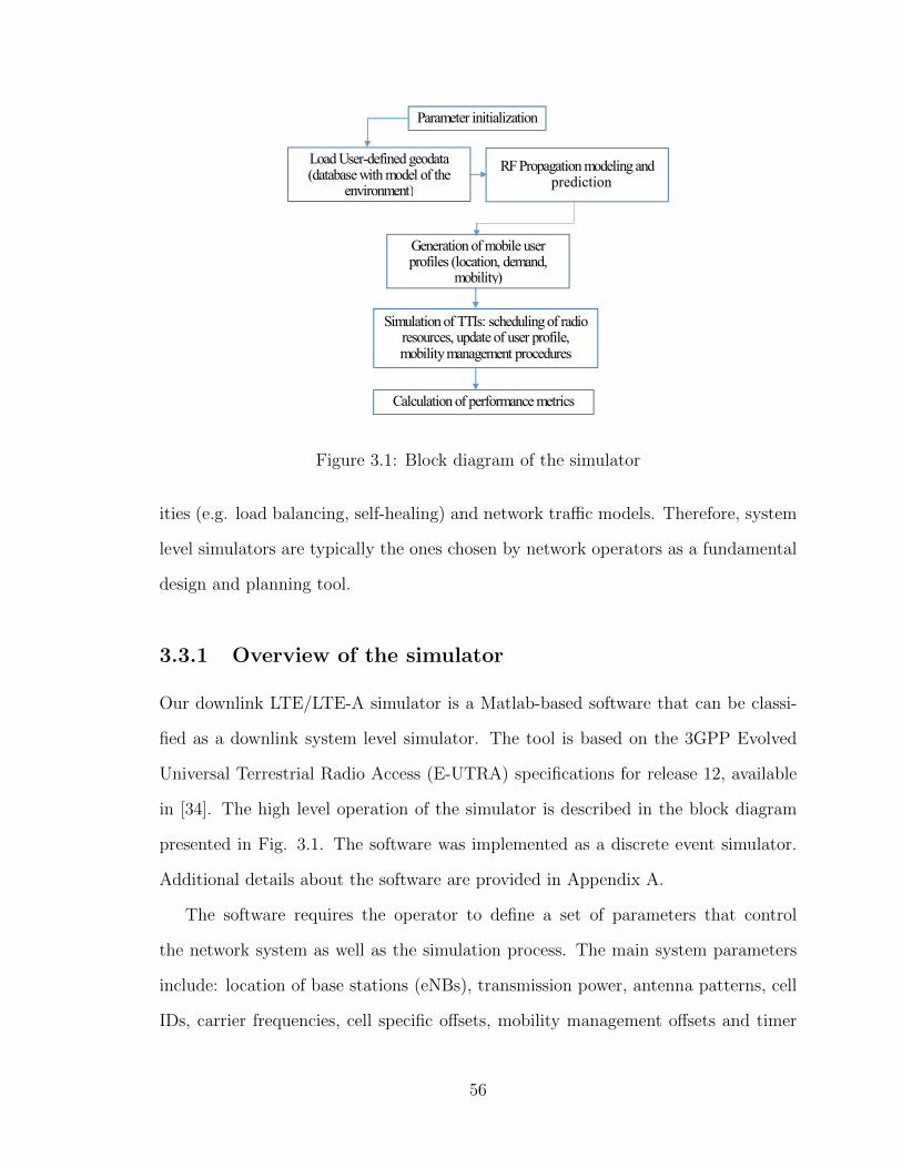
Parameter initialization

Load User-defined geodata(database with model of the

environment)

RF Propagation modeling andprediction

Generation of mobile userprofiles (location, demand,

mobility)

Simulation of TTIs: scheduling of radioresources, update of user profile,mobility management procedures

Calculation of performance metrics

Figure 3.1: Block diagram of the simulator

ities (e.g. load balancing, self-healing) and network traffic models. Therefore, system

level simulators are typically the ones chosen by network operators as a fundamental

design and planning tool.

3.3.1 Overview of the simulator

Our downlink LTE/LTE-A simulator is a Matlab-based software that can be classi-

fied as a downlink system level simulator. The tool is based on the 3GPP Evolved

Universal Terrestrial Radio Access (E-UTRA) specifications for release 12, available

in [34]. The high level operation of the simulator is described in the block diagram

presented in Fig. 3.1. The software was implemented as a discrete event simulator.

Additional details about the software are provided in Appendix A.

The software requires the operator to define a set of parameters that control

the network system as well as the simulation process. The main system parameters

include: location of base stations (eNBs), transmission power, antenna patterns, cell

IDs, carrier frequencies, cell specific offsets, mobility management offsets and timer

56

values (e.g. time-to-trigger timer), system bandwidth, MIMO configuration, cyclic

prefix length. The main simulation parameters include: duration of simulated time,

mobile spatial distribution model, selection of traffic model, speed of mobile users,

selection of mobility model, spatial resolution of the path loss predictions.

Once the parameters have been defined, the software proceeds to pre-calculate

path loss estimations for all cell sites as well as the SINR values at every location in the

map (according to the resolution value defined by the operator). These values are pre-

calculated for the whole area of interest in order to reduce computational time, these

estimations can be saved and loaded for future runs of the simulator. At this point,

the software generates mobile user profiles. Each profile includes aspects like the

location of the mobile user, its traffic demand, speed, direction of movement, serving

cell, etc. For each mobile user, the SINR conditions define the modulation order

and coding rate used to communicate with the serving base station. The measured

SINR is mapped to CQI value and the corresponding modulation and coding scheme

is selected according to the standard. The SINR-to-CQI mapping applied in our

simulations corresponds to the mapping derived in [81] for a 10% block error rate

(BLER).

Where SINRi j is the ratio of the received power from the jth eNB and the to-

tal power of the received interference from neighboring cells belonging to the same

tier plus noise. The function f (·) has been traditionally determined by the Shannon

Hartley theorem, as shown in [27,28,33,36,37]. However, in real networks bi j depends

on the value of the Channel Quality Indicator (CQI) that is periodically reported by

the user equipment (UE). The higher the measured SINRi j , the higher the value of

CQI; which means that the UE is capable of decoding received data with a higher

modulation order and coding rate. Furthermore, the spectral efficiency can also be

improved if the eNB and the UE support MIMO capabilities like spatial multiplex-

ing. The actual mapping between the measured SINRi j and the reported CQI value

57

depends on UE capabilities and have been left by the 3GPP as a vendor specific

implementation. In this study, our simulator uses the mapping derived in [81] for a

10% block error rate (BLER).

Finally, the software simulates each transmission time interval (TTI) in the net-

work. In LTE networks one TTI corresponds to 1 ms. During each TTI a scheduler

algorithm is run for each cell site and the profile of each mobile user is updated. In

the next subsections a brief description of the main components of the simulator are

provided.

3.3.2 Propagation path loss predictions

The propagation prediction model implemented in the simulator is a site-specific

propagation model described in chapter 2 and initially proposed in [56]. This model

is intended for the prediction of received signal power in outdoor environments. The

model is based on ray tracing principles and the classical (UTD). This model supports

the calculation of path losses from multiple rays reaching the receiver due to different

propagation mechanisms, including line-of-sight propagation, reflections, over-rooftop

diffractions, vertical-edge diffractions and scattering losses due to the presence of

vegetation. For receivers located indoors, the user can define a value of penetration

loss in dB/m to roughly estimate the received signal strength inside buildings. The

propagation losses are predicted for every location in the map and for every base

station defined by the operator. It is important to mention that if highly detailed

indoor propagation predictions are required, they can be imported and integrated in

the simulation from commercially available software like iBwave.

58

3.3.3 Spatial Distribution of mobile users

The initial distribution of mobile users, also known as user equipment (UE), is based

on the model selected by the user. Four models are supported:

1. Uniform distribution: all UEs are randomly distributed in the map, this is one

of the simplest distribution models.

2. Hotspot: A certain percentage of UEs (usually around 80%) are placed in the

neighboring area of a cell site, the rest are randomly distributed in the map.

This distribution model is useful for the simulation of HetNets involving small

cells, like microcells or picocells, deployed to provide service to high traffic

hotspots.

3. Traffic map: the user can define a traffic map, which consists of a partition of

the area of interest in regions. The operators can then define the percentage

of mobile users to be randomly placed inside every region. This model is very

realistic in the sense that operators can apply their knowledge about mobile

user density and spatial distribution when creating the traffic map.

3.3.4 Mobility models

To emulate the movement of users, in particular pedestrians, the simulator supports

the following mobility models:

1. Static: the simulator considers all mobile users as static for the entire duration

of the simulation time.

2. Bouncing circle: the user can define a circular region in the map. Then mobile

users will move inside the circle with random (or fixed) speed and direction of

movement. When a mobile user reaches the boundary of the circular region

59

a new direction of movement is selected such that it bounces back inside the

circle.

3. Predefined trajectories: Operators can manually define a set of trajectories

based on their knowledge about how users move in a particular place. Each

manually defined trajectory consists of a set of points (described by latitude

and longitude) that a mobile user follows. In order to model the random nature

of the movement of actual mobile users, we define a small circle of radius r

centered at each manually defined point in each trajectory. Then, each mobile

user moves between points that are randomly selected within each one of the

circles. The larger the value of r, the higher the randomness of the paths. This

model is particularly useful because it allows operators to control the places

where users move, like sidewalks or hallways, and effectively simulate the walk

test process.

3.3.5 Traffic models

The performance of the mobile network is highly dependent on the amount and type

of traffic that mobile users request. Therefore, accurate traffic models are essen-

tial to determine if a particular design or network topology will provide the desired

performance. Our simulator supports the following traffic models:

1. Full buffer: there is an infinite amount of data to be delivered to each UE, i.e.

each mobile user is actively connected during the entire simulation period and

it is always receiving data. This model is typically used as a worst case scenario

to determine the lower bounds of the performance of the network under extreme

load conditions.

2. Finite buffer: the amount of data to be delivered to any UE is not infinite, each

mobile user is expecting to receive a specific amount of data. The total data

60

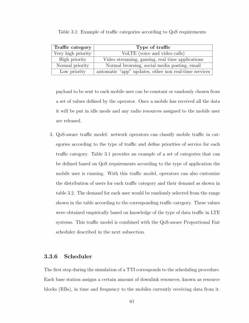
Table 3.1: Example of traffic categories according to QoS requirements

Traffic category Type of trafficVery high priority VoLTE (voice and video calls)

High priority Video streaming, gaming, real time applicationsNormal priority Normal browsing, social media posting, email

Low priority automatic “app” updates, other non real-time services

payload to be sent to each mobile user can be constant or randomly chosen from

a set of values defined by the operator. Once a mobile has received all the data

it will be put in idle mode and any radio resources assigned to the mobile user

are released.

3. QoS-aware traffic model: network operators can classify mobile traffic in cat-

egories according to the type of traffic and define priorities of service for each

traffic category. Table 3.1 provides an example of a set of categories that can

be defined based on QoS requirements according to the type of application the

mobile user is running. With this traffic model, operators can also customize

the distribution of users for each traffic category and their demand as shown in

table 3.2. The demand for each user would be randomly selected from the range

shown in the table according to the corresponding traffic category. These values

were obtained empirically based on knowledge of the type of data traffic in LTE

systems. This traffic model is combined with the QoS-aware Proportional Fair

scheduler described in the next subsection.

3.3.6 Scheduler

The first step during the simulation of a TTI corresponds to the scheduling procedure.

Each base station assigns a certain amount of downlink resources, known as resource

blocks (RBs), in time and frequency to the mobiles currently receiving data from it.

61

One resource block in LTE systems has a duration of one TTI and corresponds to

a set of 12 consecutive subcarriers with a total bandwidth of 180 KHz per RB. The

scheduler is the algorithm that defines the rules for this assignment. Two scheduling

algorithms are supported by our simulator, we describe them below.

1. Proportional Fair (PF): this is a well-known scheduling algorithm and very

popular in OFDMA-based systems like LTE [82]. The PF algorithm assigns

resource blocks to UEs according to a priority score or metric Mi,k (n), where i

and k are the UE and RB identifier respectively, and n is the TTI period. The

metric is calculated according to (3.1).

Mi,k (n) =ri,k (n)Ri (n)

, i ∈ Ik (n) (3.1)

Where ri,k (n) is the rate UE i would receive if RB k is scheduled to it in TTI n,

Ri (n) is the long-term average rate for UE i and Ik (n) is the set of UEs eligible

to compete for the RB k in this TTI. The long-term rate is typically calculated

with an exponential moving average filter. The resource block is assigned to

the user with highest metric Mi,k (n).

With this scheduling algorithm, UEs with poor RF conditions will be assigned

more RBs to satisfy their demand so that they can achieve fair rates compared

to those UEs with good RF conditions (that only need a small number of RBs

to satisfy their demand).

2. QoS aware-PF scheduler: If the QoS-aware traffic model is selected, the clas-

sical PF scheduler is modified to account for the fact that users are classified

according to different traffic priorities. For instance, it is expected that users

with Very high priority traffic should have a higher chance of receiving down-

link resources than those users with a lower priority traffic. Therefore, we have

62

Table 3.2: Example of scheduling probabilities, percentage of users and expected datarates for each traffic category

Traffic category Scheduling probability P Percentage of users Demanded rateVery high 0.85 5% [10,20] Mbps

High 0.75 20% 30 Mbps or higherNormal 0.5 35% [15,30] Mbps

Low 0.3 40% [5,30] Mbps

proposed to modify the set Ik (n) in (3.1) for every scheduling decision for each

RB. In the classical PF algorithm, all connected UEs are allowed to compete for

RB k at TTI n. With the QoS-aware traffic model, we define a set of scheduling

probabilities associated with each traffic category. Table 3.2 shows an example

of these probabilities. We propose to calculate the set Ik (n) for each RB k as:

Ik (n) = {i ∈ I|Pi > gk (n)} (3.2)

Where the set I contains all the UEs expecting downlink resources, Pi is the

scheduling probability of user i according to their traffic category as shown in

table 3.2 and gk (n) is a random number generated from a uniform distribution

in the interval [0,1]. With (3.2), users with high traffic priority are more likely

to be selected to compete for downlink resources than those users with lower

scheduling probability. Therefore, this scheduling algorithm first selects the

users in I, then computes the values of the metric Mi,k (n) for each one of them

and finally it schedules RB k to the UE with highest value of the metric Mi,k (n).

3.3.7 Mobility Management

The intra-frequency handover for connected users in 3GPP systems consists of four

main phases [34]: measurement, processing, preparation, and execution. UEs contin-

uously monitor the received signal strength from their serving base station (SeNB)

63

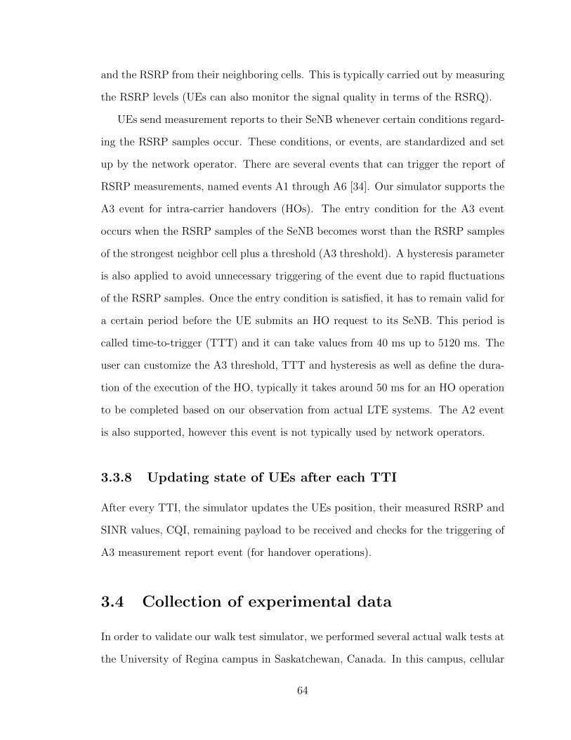
and the RSRP from their neighboring cells. This is typically carried out by measuring

the RSRP levels (UEs can also monitor the signal quality in terms of the RSRQ).

UEs send measurement reports to their SeNB whenever certain conditions regard-

ing the RSRP samples occur. These conditions, or events, are standardized and set

up by the network operator. There are several events that can trigger the report of

RSRP measurements, named events A1 through A6 [34]. Our simulator supports the

A3 event for intra-carrier handovers (HOs). The entry condition for the A3 event

occurs when the RSRP samples of the SeNB becomes worst than the RSRP samples

of the strongest neighbor cell plus a threshold (A3 threshold). A hysteresis parameter

is also applied to avoid unnecessary triggering of the event due to rapid fluctuations

of the RSRP samples. Once the entry condition is satisfied, it has to remain valid for

a certain period before the UE submits an HO request to its SeNB. This period is

called time-to-trigger (TTT) and it can take values from 40 ms up to 5120 ms. The

user can customize the A3 threshold, TTT and hysteresis as well as define the dura-

tion of the execution of the HO, typically it takes around 50 ms for an HO operation

to be completed based on our observation from actual LTE systems. The A2 event

is also supported, however this event is not typically used by network operators.

3.3.8 Updating state of UEs after each TTI

After every TTI, the simulator updates the UEs position, their measured RSRP and

SINR values, CQI, remaining payload to be received and checks for the triggering of

A3 measurement report event (for handover operations).

3.4 Collection of experimental data

In order to validate our walk test simulator, we performed several actual walk tests at

the University of Regina campus in Saskatchewan, Canada. In this campus, cellular

64

SECTOR 1

SECTOR 2SECTOR 3

Start

end

Figure 3.2: Sectors of the macrocell covering campus as well as example of trajectoryfollowed during the walk tests

service is primarily provided by a 3-sector LTE macrocell system operating at 2.1

GHz with 20 MHz bandwidth, the macrocell also provides service to the surrounding

residential areas. We selected a specific trajectory that is typically followed by a large

number of students, faculty and staff during the day.

Furthermore, this trajectory goes through the handover region between two of

the sectors of the macrocell. The handover happens from Sector 3 to Sector 2 as

shown in Fig. 3.2. Therefore, the results of the walk test can be used to evaluate the

performance of the system as connected users are handed over from one sector to the

other. This will also allow us to evaluate the accuracy of our simulation tool and its

capability to model this essential characteristic of mobile networks.

It is important to mention that Sector 2 covers most of the campus area, while

Sector 3 covers only a small portion of the campus but a large portion of the sur-

rounding residential areas. The walk tests were carried out under three different load

conditions of the network during a weekday:

1. Scenario 1: Early morning, students and staff arriving to campus, residents

65

of surrounding areas are off to work. Typically both sectors have around 40

connected users.

2. Scenario 2: Noon, peak usage during lunch hour. Sector 2 is usually highly

loaded with around 100 connected users, while Sector 3 has lower load of around

60 users.

3. Scenario 3: Evening, most staff members and students have left campus, resi-

dents of surrounding areas are back from work. Sector 2 becomes lightly loaded

with an average of 40 connected users but more users connect to Sector 3,

reaching an average of 70 during this time.

During each walk test, a downlink speed test was carried out. The speed tests

consisted of downloading a large file from an FTP server that is directly connected to

the Core network of the mobile system operator. The walk was repeated 30 times and

data like RSRP and SINR from the serving sector, downlink data rate and serving

cell ID were logged.

An Android-based application called Nemo Walker Air, developed by Anite Inc.

was used to perform the measurement and logging of the walk test data. This appli-

cation was installed on a Sony Xperia Z3 phone. Measurements were logged at a rate

of approximately 300ms.

The data collected from each walk test was averaged after aligning the data in

time using as a reference the execution of the handover between sectors. In Fig.

3.3, we provide an example of the average measured RSRP values during scenario 3.

Note that the horizontal axis represents time and t = 0 indicates the time when the

handover was completed, similarly for Figs. 3.4 to 3.7.

66

3.5 Results & Analysis

In this section we present the results of the validation of our walk test simulator.

3.5.1 RSRP and SINR estimations

In Fig. 3.3 and 3.4 we provide an example of the measured values of RSRP and SINR

corresponding to scenario 3. Time t = 0 in the horizontal axis indicates the completion

of the handover. The edge of both sectors is clearly shown in both figures. The values

of RSRP decreased from -72 dBm in the service area of Sector 3 and decreased to a

value close to -80 dBm right at the moment of the execution of the handover to Sector

2. A similar behavior is observed for the SINR plot in Fig. 3.4, where very low values

of SINR are observed at the cell edge. It is important to mention that our simulator

provided a similar trend as the experimental data. The mean error and mean absolute

errors were computed for every tested scenario, table 3.3 shows the results (a negative

mean error indicates a over-estimation). The overall average of the mean error of the

RSRP estimations was -1.22 dBm and the overall average of the mean absolute error

was 2.3 dBm. Regarding the SINR estimations, the overall average of the mean error

was -0.48 dBm and the overall average of the mean absolute error was 2.25 dBm.

Based on these results it is clear that our modeling of the physical environment and

the propagation of radio frequency signals is relatively accurate.

3.5.2 Downlink data rate

Fig. 3.5, 3.6 and 3.7 show the average data rate measured during our actual walk tests

under the three different scenarios described in 3.4 (once again, time t = 0 indicates

the completion of the handover). We also include our simulation results using two

different traffic models: Full Buffer and QoS-aware, note that during our simulation

the sectors were loaded according to the number of users described in Sect. 3.4. The

67

−50 −40 −30 −20 −10 0 10 20 30 40 50−82

−80

−78

−76

−74

−72

−70

−68

−66

−64

Time (s)

RS

RP

(dB

m)

Experimental dataSimulation

Figure 3.3: Example of the RSRP measured and estimated for scenario 3

−50 −40 −30 −20 −10 0 10 20 30 40 50

0

5

10

15

Time (s)

SIN

R (

dB)

Experimental dataSimulation

Figure 3.4: Example of the SINR measured and estimated for scenario 3

Table 3.3: Mean error and mean absolute error of RSRP and SINR estimations.Standard deviation is shown between brackets, all units in dBm

RSRPScenario 1 2 3

Mean Error -1.32 (3.5) -0.85 (2.9) -1.5 (2.3)Mean Absolute Error 2.72 (2.6) 2.2 (2.1) 1.9 (1.95)

SINRScenario 1 2 3

Mean Error 0.93 (2.5) -1.43 (2.8) -0.94 (2.43)Mean Absolute Error 2.04 (1.8) 2.5 (1.94) 2.22 (1.35)

QoS-aware traffic model was setup with the parameters from table 3.2.

Fig. 3.5 corresponds to the case when both sectors are lightly loaded early morn-

ing. In this case, during our test we were able to measure a significantly high data

68

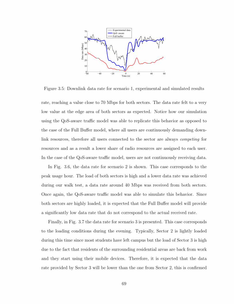
−60 −40 −20 0 20 40 600

10

20

30

40

50

60

70

Time (s)

Dat

a ra

te (

Mbp

s)

Experimental dataQoS−awareFull buffer

Figure 3.5: Downlink data rate for scenario 1, experimental and simulated results

rate, reaching a value close to 70 Mbps for both sectors. The data rate felt to a very

low value at the edge area of both sectors as expected. Notice how our simulation

using the QoS-aware traffic model was able to replicate this behavior as opposed to

the case of the Full Buffer model, where all users are continuously demanding down-

link resources, therefore all users connected to the sector are always competing for

resources and as a result a lower share of radio resources are assigned to each user.

In the case of the QoS-aware traffic model, users are not continuously receiving data.

In Fig. 3.6, the data rate for scenario 2 is shown. This case corresponds to the

peak usage hour. The load of both sectors is high and a lower data rate was achieved

during our walk test, a data rate around 40 Mbps was received from both sectors.

Once again, the QoS-aware traffic model was able to simulate this behavior. Since

both sectors are highly loaded, it is expected that the Full Buffer model will provide

a significantly low data rate that do not correspond to the actual received rate.

Finally, in Fig. 3.7 the data rate for scenario 3 is presented. This case corresponds

to the loading conditions during the evening. Typically, Sector 2 is lightly loaded

during this time since most students have left campus but the load of Sector 3 is high

due to the fact that residents of the surrounding residential areas are back from work

and they start using their mobile devices. Therefore, it is expected that the data

rate provided by Sector 3 will be lower than the one from Sector 2, this is confirmed

69

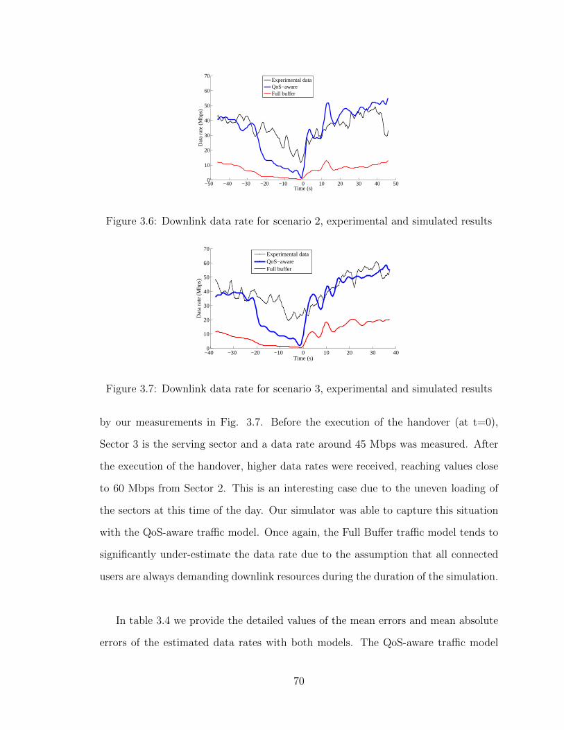
−50 −40 −30 −20 −10 0 10 20 30 40 500

10

20

30

40

50

60

70

Time (s)

Dat

a ra

te (

Mbp

s)

Experimental dataQoS−awareFull buffer

Figure 3.6: Downlink data rate for scenario 2, experimental and simulated results

−40 −30 −20 −10 0 10 20 30 400

10

20

30

40

50

60

70

Time (s)

Dat

a ra

te (

Mbp

s)

Experimental dataQoS−awareFull buffer

Figure 3.7: Downlink data rate for scenario 3, experimental and simulated results

by our measurements in Fig. 3.7. Before the execution of the handover (at t=0),

Sector 3 is the serving sector and a data rate around 45 Mbps was measured. After

the execution of the handover, higher data rates were received, reaching values close

to 60 Mbps from Sector 2. This is an interesting case due to the uneven loading of

the sectors at this time of the day. Our simulator was able to capture this situation

with the QoS-aware traffic model. Once again, the Full Buffer traffic model tends to

significantly under-estimate the data rate due to the assumption that all connected

users are always demanding downlink resources during the duration of the simulation.

In table 3.4 we provide the detailed values of the mean errors and mean absolute

errors of the estimated data rates with both models. The QoS-aware traffic model

70

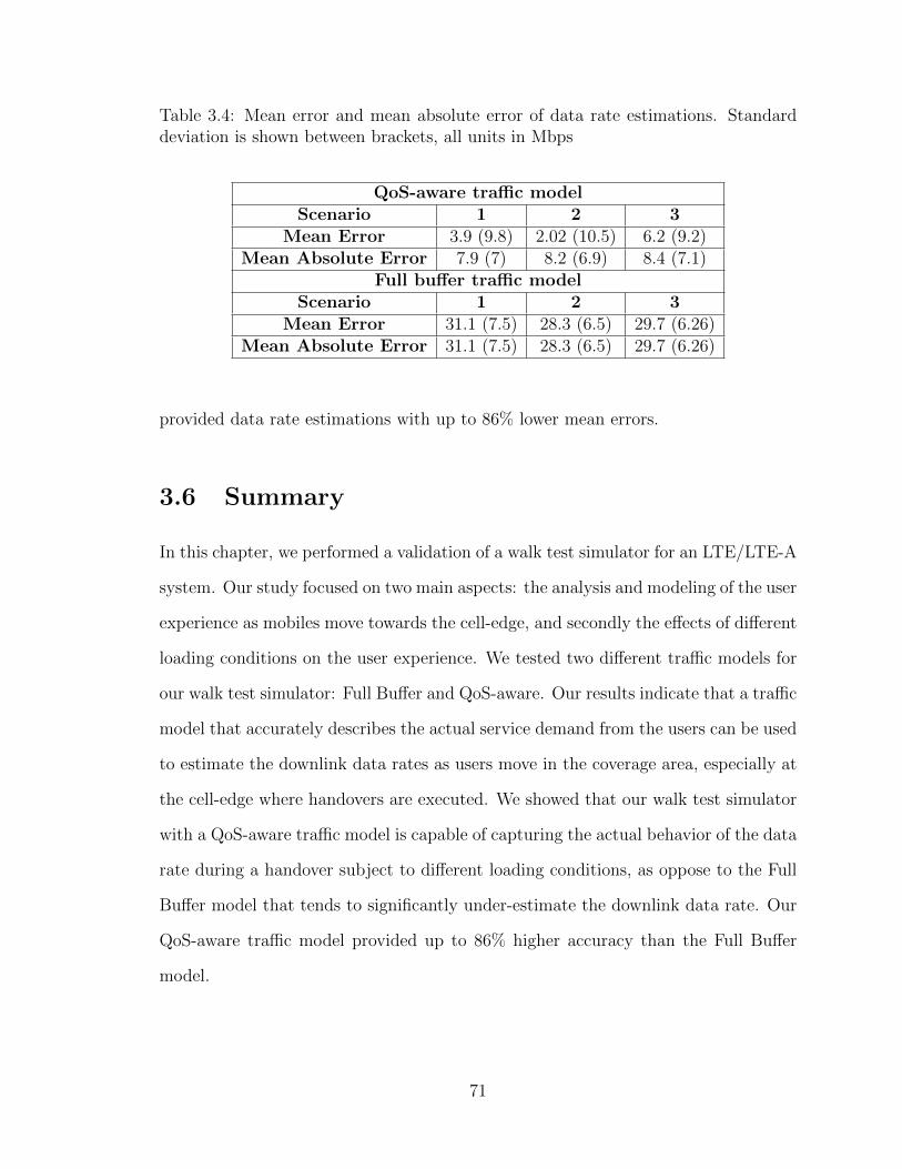
Table 3.4: Mean error and mean absolute error of data rate estimations. Standarddeviation is shown between brackets, all units in Mbps

QoS-aware traffic modelScenario 1 2 3

Mean Error 3.9 (9.8) 2.02 (10.5) 6.2 (9.2)Mean Absolute Error 7.9 (7) 8.2 (6.9) 8.4 (7.1)

Full buffer traffic modelScenario 1 2 3

Mean Error 31.1 (7.5) 28.3 (6.5) 29.7 (6.26)Mean Absolute Error 31.1 (7.5) 28.3 (6.5) 29.7 (6.26)

provided data rate estimations with up to 86% lower mean errors.

3.6 Summary

In this chapter, we performed a validation of a walk test simulator for an LTE/LTE-A

system. Our study focused on two main aspects: the analysis and modeling of the user

experience as mobiles move towards the cell-edge, and secondly the effects of different

loading conditions on the user experience. We tested two different traffic models for

our walk test simulator: Full Buffer and QoS-aware. Our results indicate that a traffic

model that accurately describes the actual service demand from the users can be used

to estimate the downlink data rates as users move in the coverage area, especially at

the cell-edge where handovers are executed. We showed that our walk test simulator

with a QoS-aware traffic model is capable of capturing the actual behavior of the data

rate during a handover subject to different loading conditions, as oppose to the Full

Buffer model that tends to significantly under-estimate the downlink data rate. Our

QoS-aware traffic model provided up to 86% higher accuracy than the Full Buffer

model.

71

Chapter 4

A Distributed Load BalancingAlgorithm for Heterogeneous

Networks

In this chapter, we propose a practical distributed load balancing algorithm for

LTE/LTE-A heterogeneous networks. We have formulated the problem as a local

sum utility maximization. The distributed algorithm is capable of fairly distributing

the load among base stations with a reduced level of coordination. The evaluation

of our load balancing algorithm was carried out through a comparative analysis with

other two near-optimal load balancing algorithms based on convex optimization. We

evaluated the capacity of the algorithms to provide effective offloading capabilities,

fairness of the distribution of the load among base stations and downlink data rate

gains. We also evaluated the practicality of these algorithms in terms of the required

amount of coordination and exchange of information among base stations (e.g. han-

dover triggering). An excessive exchange of signaling messages is undesired and could

lead to an increase in power consumption at the base station level. Additionally, an

excesive number of handovers is undesirable and can negatively affect user experience.

This type of analysis has usually been overlooked in past studies. We tested these

algorithms in a typical HetNet deployment in a university campus, subject to realis-

tic traffic and load distribution. Our results show that our load balancing algorithm

was able to provide similar data rate gains compared to the other two algorithms,

however our approach is substantially less complex. Additionally, our load balancing

algorithm was superior in terms of its practicality due to a significantly low required

level of coordination and exchange of information across base stations.

72

4.1 Introduction

HetNet deployments can bring great advantages for network operators and sub-

scribers. However, there are important challenges to consider when it comes to opti-

mizing their performance. One key challenge is the increasing complexity of network

planning, in particular as the density of small cells per macrocell increases.

Furthermore, another relevant challenge is related to the balancing of the load

across base stations. HetNets are an excellent option for increasing capacity and

decreasing congestion levels of macrocells during peak periods. However, careful

coordination among base stations is necessary to achieve a fair distribution of the

traffic. User experience can be significantly affected when receiving service from

an overloaded base station, even in areas with high SINR conditions. Current cell

selection mechanisms, e.g. a user is served by the base station that provides the

strongest received signal (a scheme known as the max-RSRP in LTE systems), tend

to ignore a critical aspect: the load of the base stations [33]. These mechanisms

provide suboptimal cell associations with unbalanced load distributions, leading to

congestion in some cells and under-utilization in others. Sharing the load among

base stations (small cells and macrocells), can greatly improve the overall network

throughput.

Typically, small cells are strategically placed to provide service to high-traffic

areas, known as traffic hotspot. Due to the disparity in transmission power between

the small cells and the tower-mounted macrocell, it is not uncommon for mobiles

located in the hotspot zone to receive the strongest downlink signal from the macrocell

[27]. As a result, microcells and picocells will typically be under-loaded and an active

mechanism is necessary to encourage mobiles to select any of the small cells as their

serving base station. This active mechanism should be designed in such a way that

it is capable of fairly distributing the load among all base stations, while providing

73

a satisfactory quality of service for all users, in particular for those mobiles located

at the cell-edge. Additionally, such load balancing mechanism should minimize the

overhead cost (in terms of coordination among base stations), as well as reduce the

number of triggered handovers to avoid a negative impact in the signaling load of the

network.

In this chapter, we propose a distributed load balancing algorithm based on traffic

transfer with reduced signaling exchange between eNBs. Given a current suboptimal

user association, each base station can solve locally a load-aware utility maximization

problem. Such problem is solved based on the information of the current eNB’s load

level, resource scheduling and SINR conditions of its associated users. By solving the

utility maximization problem locally, an overloaded base station can determine which

users are negatively impacting its sum of the utility, those users are then candidates

to be transferred to other base stations with spare capacity via load-aware handover

procedures.

The performance of the load balancing algorithm proposed in this chapter was

evaluated through a comparative analysis considering other two near-optimal load

balancing algorithms. The other two algorithms considered in this study are the

ones proposed by Ye et al. in [27], by Shen and Yu in [28]. The evaluation scenario

consisted of a typical HetNet deployment in a university campus venue under realistic

traffic and load conditions. Our results confirmed the benefits of balancing the load in

HetNets. Significant data rate gains were achieved by all three algorithms. However,

our load balancing algorithm is substantially superior in terms of its practicality due

to a lower amount of exchange of information among eNBs as well as a low number

of required handovers.

The chapter is organized as follows: in Sect. 4.2 we provide an overview of the

research work in this area. In Sect. 4.3 we describe the system model. Sect. 4.4

provides details about the mathematical formulation of the load balancing problem,

74

and we also provide a description of our algorithm as well as the load balancing

algorithms described in [27] and [28]. We describe the performance evaluation of the

our load balancing algorithm in Sect. 4.5. Finally, in Sect. 4.6 we provide a brief

summary of this chapter.

4.2 Related work

Significant efforts have been made to propose effective load balancing algorithms

based on traffic transfer strategies. The use of adaptive cell specific offsets, or Range

Extension Bias (REB), to dynamically control the coverage areas of small cells has

been extensively studied [36–41]. With this mechanism, a mobile will add the value

of the bias to the received signal power from a picocell or microcell to “artificially”

increase the power of the small cell, hence this encourages the mobile to select it as

its serving cell as opposed to the macrocell (when the max-RSRP scheme is applied).

Unfortunately, the optimal values of REB are typically calculated based on network-

wide analysis, with bias values specified in a per-tier basis and typically applying

centralized algorithms with slow adaptation. Additionally, these approaches tend to

ignore the fact that users in the range extended area are subject to higher interference

levels and a degradation of the service is expected for those users.

For example, in [36], the authors applied a linear regression-based scheme to

predict a value of the REB with the objective of balancing the load between a picocell

and a macrocell. Their approach consists of the application of a path loss equation

to calculate a “virtual distance” (VD) between a picocell base station and its users,

a concept that was also investigated in [41]. The set of VDs is used to fit a linear

regression model, this model is then used to predict the value of the virtual distance

that would result in a desired number of picocell users defined a priori. With such

new VD, a new value of the REB is calculated by applying the path loss equation.

75

As a result of the new REB value a set of handovers are triggered to transfer users

between the base stations. Their simulation results indicate a better load balancing

compared to the max-RSRP association rule. The approach requires the collection

of measurement reports from mobiles, additionally the concept of VD might not be

accurate enough for indoor environments or highly dense HetNets. Furthermore,

there is no consideration of the degradation in the quality of service for users in the

extended range of the small cell.

In [37], a centralized scheme is proposed to determine suitable values of the REB.

The REB calculation is based on an optimization problem (similarly as in [40]). The

optimization problem is defined in terms of a set of non-linear equations (intended to

model the coupled nature of the load among base stations in the network), this system

of equations include the Jain’s fairness index (see (4.19)). In order to approximate

the solution to this maximization problem, the authors apply the principle of Design

of Experiments (DOE). This is an iterative and statistical approach used to evaluate

the effects of multiple factors simultaneously and determine the most relevant ones.

According to their simulation results, a fairness index of 0.9 can be achieved (a fairness

index closer to unity indicates a fairer load distribution). This approach has the key

disadvantage of being a network-wide centralized approach, this means that tight

coordination among all base stations in the network is required.

The authors in [38,39] proposed the adjustment of the REB based on incremental

steps in order to keep certain performance metrics above a desired target. Such

metrics could include SINR distribution, downlink throughput or the ratio between

the transmission power of a base station and its connected users. A disadvantage of

these approaches is the slow adaptation of the schemes. Their simulation results show

little improvement in the throughput of cell-edge users compared to the case when a

single and static REB is applied, around 5% gain.

On the other hand, authors in [27, 28] have proposed approaching the load bal-

76

ancing issue as a convex optimization problem with the significant advantage that it

can be solved in a distributed fashion. A utility function is formulated, typically in

terms of the users achievable data rate. The optimal cell association that maximizes

the network-wide sum of the utility is found. Unique user association, power control

and load sharing are constraints included in the optimization problem. Approximat-

ing the optimal network-wide user association usually involves the implementation

of complex iterative algorithms, which require significant coordination between base

stations and a substantial exchange of signaling messages between base stations and

users (UEs). Based on their simulation results, these approaches were able to fairly

distribute the load among base stations and obtain significant gains in throughput

for cell-edge users (around 350%), this is an important improvement compared to the

REB-based approaches. A full description of these two algorithms is provided in Sect.

4.4.

The load balancing algorithm proposed in this chapter has been inspired by the

works in [27, 28]. The proposed algorithm does not require a centralized execution,

but more importantly our intention is to reduce the required coordination among

base stations. This is carried out by reducing the amount of signaling messages as

well as the number of triggered handovers. With our load balancing algorithm a base

station can solve locally a load-aware utility maximization problem. We propose to

approximate the solution to the optimization problem with a heuristic method that

requires information that is available locally at the base station level (e.g. load level,

resource scheduling and SINR conditions of its associated users). This approach does

not require the update of the network-wide cell association after every iteration, as

it is done in [27, 28]. Such step significantly increases the number of handovers and

the exchange of messages among base stations.

77

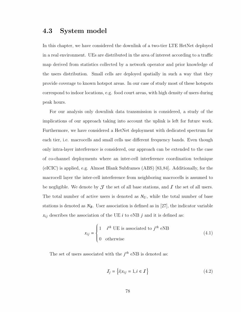
4.3 System model

In this chapter, we have considered the downlink of a two-tier LTE HetNet deployed

in a real environment. UEs are distributed in the area of interest according to a traffic

map derived from statistics collected by a network operator and prior knowledge of

the users distribution. Small cells are deployed spatially in such a way that they

provide coverage to known hotspot areas. In our case of study most of these hotspots

correspond to indoor locations, e.g. food court areas, with high density of users during

peak hours.

For our analysis only downlink data transmission is considered, a study of the

implications of our approach taking into account the uplink is left for future work.

Furthermore, we have considered a HetNet deployment with dedicated spectrum for

each tier, i.e. macrocells and small cells use different frequency bands. Even though

only intra-layer interference is considered, our approach can be extended to the case

of co-channel deployments where an inter-cell interference coordination technique

(eICIC) is applied, e.g. Almost Blank Subframes (ABS) [83,84]. Additionally, for the

macrocell layer the inter-cell interference from neighboring macrocells is assumed to

be negligible. We denote by J the set of all base stations, and I the set of all users.

The total number of active users is denoted as NU , while the total number of base

stations is denoted as NB. User association is defined as in [27], the indicator variable

xi j describes the association of the UE i to eNB j and it is defined as:

xi j =

1 ith UE is associated to jth eNB

0 otherwise

(4.1)

The set of users associated with the jth eNB is denoted as:

Ij ={i |xi j = 1, i ∈ I

}(4.2)

78

The instantaneous downlink data rate offered by the jth eNB to the ith user, during

subframe k is defined as:

ri j (k) = ωoi j (k) · bi j (k) (4.3)

Where ωoi j (k) is the bandwidth in Hz scheduled (offered) for downlink transmissions

to the ith UE. The value bi j (k) corresponds to the normalized rate of the UE in b/s/Hz

and is, in general, a function of the SINRi j as:

bi j = f (SINRi j ) (4.4)

Where SINRi j is the ratio of the received power from the jth eNB and the total power

of the received interference from neighboring cells belonging to the same tier plus

noise. The function f (·) has been traditionally determined by the Shannon Hartley

theorem, as shown in [27,28,33,36,37]. However, in real networks bi j depends on the

value of the Channel Quality Indicator (CQI) that is periodically reported by the UE.

The higher the measured SINRi j , the higher the value of CQI; which means that the

UE is capable of decoding received data with a higher modulation order and coding

rate. Furthermore, the spectral efficiency can also be improved if the eNB and the UE

support MIMO capabilities like spatial multiplexing. The actual mapping between

the measured SINRi j and the reported CQI value depends on UE capabilities and

have been left by the 3GPP as a vendor specific implementation. In this study, our

simulator uses the mapping derived in [81] for a 10% block error rate (BLER).

The long-term rate of user i is calculated as the average of the instantaneous rate

during a certain number of subframes K :

Ri j =

K∑k=1

ri j (k)K

(4.5)

79

4.3.1 Load of eNBs

In an LTE/LTE-A network, all active UEs that connect to an eNB have to share

the available bandwidth. Each one of the UEs demands a specific quality of service

depending on the running application. Low bandwidth demand may correspond to

voice calls or downloading small files, whereas bandwidth intensive applications like

HD video streaming or gaming, requires higher demand of resources. The task of the

scheduler is to distribute the available bandwidth such that the demanded quality of

service of each user is satisfied, while keeping a sense of fairness.

The load of an eNB can be quantified in terms of the demanded load and the

offered load. A demanded load index and offered load index are defined as [36]:

LDj =

∑i∈Ij ω

Di j

W j(4.6)

LOj =

∑i∈Ij ω

Oi j

W j(4.7)

Where ωOi j and ωD

i j are the average offered and demanded bandwidth of the ith

user respectively during K subframes, and W j corresponds to the total bandwidth of

the jth eNB. The offered load index LOj reaches its maximum value of one when the

totality of the bandwidth have been scheduled for downlink transmissions. On the

other hand, the demanded load index LDj can take values larger than 1, e.g. when

the total demand of bandwidth is higher than the available bandwidth.

A base station whose offered load index is below unity is assumed to be under-

loaded since a portion of its bandwidth has not been scheduled, hence it has spare

capacity. However, when the offered load index approaches unity and the demanded

load index is above unity, then the base station is considered to be overloaded, since

it does not have enough resources to satisfy its current demand. The sum throughput

of a base station can be greatly impacted by the overload condition, resulting in a

80

degraded quality of service. A situation that is undesirable for network operators.

4.4 Problem formulation and description of load

balancing algorithms

The goal of an effective load balancing algorithm is to balance the overall load in the

network between eNBs. Typically, network-wide optimization techniques have been

proposed to solve the load balancing problem [27,28]. Based on the long-term rate of

the ith user, a utility function Ui (Ri j ) is calculated and a network-wide optimization

problem is formulated to find the optimal user association:

X = arg maxX

∑i∈I

∑j∈J

xi j ·Ui (Ri j )

s.t.∑j∈J

xi j = 1,∀i ∈ I

xi j ∈ {0, 1},∀i ∈ I,∀ j ∈ J

(4.8)

With X = {xi j |i ∈ I, j ∈ J } being the network-wide user association. The ob-

jective is to find the optimal distribution of UEs X among all the eNBs subject to

the constraint that any UE has to be associated to only one eNB. The optimal cell

association provides the maximum sum of the utilities of all the users in the network.

As it has been mentioned in [27, 28], the optimization defined in (4.8) is a combina-

torial problem whose computation is intractable for real size networks. The problem

becomes more challenging due to the coupled relationship between the load of each

eNB and the user association, since the long term rate Ri j depends on how loaded

the jth eNB is. Different authors have proposed relaxations to reduce the complexity

of the optimization problem, e.g. in [27] a fractional user association scheme allows

a user to be associated with more than one base station. Additionally, significant

efforts have been made to solve (4.8) in a distributed manner [28]. Unfortunately,

many of the proposed methods require high coordination between base stations and

81

a significant amount of exchange of messages between users and eNBs.

Our load balancing algorithm based on a local optimization method (LOM) is pre-

sented below. Additionally, for comparison purposes we also provide in this section

a brief description of two other load balancing algorithms based on convex optimiza-

tion. These algorithms were proposed by Ye et al. in [27] and by Shen and Yu in [28].

Both these algorithms approximate the solution to the problem formulated in (4.8)

by applying Lagrangian dual decomposition analysis. The algorithm proposed in [27]

is based on the subgradient method (SGM), and the one proposed in [28] is based on

the dual coordinate descend method (DCD).

4.4.1 Load balancing algorithm based on local optimization(LOM)

In this subsection, we describe our load balancing algorithm, initially proposed in

[57]. Instead of solving the network-wide optimization problem stated in (4.8), we

simplify the problem by letting each base station determine its own local optimal

user association, imposing a constraint based on the desired level of demanded load.

The simplified optimization problem can be expressed in terms of a local indicator

variable xi as [57]:

X j = arg maxX j

∑i∈Ij

xi ·Ui (Ri j )

s.t.∑i∈Ij

xi · ωDi j < αW j

xi ∈ {0, 1},∀i ∈ Ij, α ≥ 1

(4.9)

With X j = { xi |i ∈ Ij }. The local optimal user association X j can be calculated by

each base station considering all the UEs currently associated to it. By solving (4.9),

each base station can select from the set of associated UEs a subset of users that

maximizes its own sum of the utility function. The optimal local user association X j

82

must also satisfy a constraint related to the desired level of demanded load, i.e. the

total demanded load of the selected users must not exceed the value αW j , where the

parameter α can take a value higher or equal than 1. A value of α closer to unity

will provide a stricter selection of UEs. Such parameter can be setup by the network

operator.

Similarly as in [27, 28], we have selected a logarithmic utility function. As it was

stated in [27], the logarithmic function has the advantage that it yields high utility

values if more resources are provided to users with low rates (cell-edge users) as

opposed to providing the same amount of resources to users already with good rates.

This encourages cell-edge users associated with overloaded eNBs to be transferred to

underloaded base stations where they can receive more resources, hence improving

the balance of the load among eNBs. In our case we define the logarithmic utility

function as:

Ui (Ri j, ωOi j ) = log *

,

Ri j

ωOi j

+-

(4.10)

The quantity Ri j/ωOi j represents the average normalized long-term rate for the ith

UE in b/s/Hz.

We approximate the solution of the problem formulated in (4.9) with an approach

based on greedy heuristics. We first start by calculating the values of the utility

function for each user associated to a base station. Then, the users are sorted in

descending order based on the corresponding value of the utility function. Starting

with the user with highest value of utility, its indicator function xi is set to “1” if

the resulting cumulative demanded load is below αW j . The rest of the users are

evaluated sequentially, and their indicator function xi will be set to “1” as long as

the total cumulative demanded load constraint is satisfied. Otherwise, the indicator

function will take the value of “0”. The pseudo-code of this process is presented in

Algorithm 4.1.

83

Algorithm 4.1 Get X j

Require: Set U = {Ui |i ∈ Ij }

Require: Set WD = {ωDi j |i ∈ Ij }

Require: Parameter α1: demanded load ← 02: Sort(U) in descending order3: for n = 1 to |Ij | do4: UEn ← Get UE(U )5: if demanded load + ωD

nj < αW j then6: xn = 17: demanded load = demanded load + ωD

nj8: else9: xn = 0

10: end if11: end for12: X j ← { xn}

Based on the set X j , the base station can determine which users are candidates to

be transferred to underloaded neighboring base stations. We define the sets Sj and

Tj as:

Sj ={i | xi = 1, xi ∈ X j

}(4.11)

Tj ={i | xi = 0, xi ∈ X j

}(4.12)

The set Sj contains the subset of users that will continue to be associated with

the jth eNB after X j has been obtained from algorithm 4.1. The set Tj contains the

subset of users that the base station will attempt to transfer to other underloaded

eNBs via handover operation.

After the sets Sj and Tj are known, it is time to actively transfer the excess load

to base stations with spare capacity. For each user in Tj , the base station should

submit a handover request to another base station with spare capacity, and whose

RSRP and SINR measured by the user satisfy the cell selection criteria defined by

the operator. The values of RSRP and SINR of neighboring cells are obtained from

84

measurements reports submitted by the users in Tj .

Evidently, the overloaded base station must know the current loading condition

level of its neighboring cells so that it can select target eNBs that are underloaded.

This information can be obtained from a centralized unit in charge of periodically

broadcasting load indicators (e.g. the offered and demanded load indexes) of all the

base stations. For our proposed algorithm, this is the only piece of information that

base stations need to share among each other. The exchange of this information is a

functionality expected to be part of self-optimizing networks (SON) [85].

It is expected that an overloaded base station might not be able to transfer all the

users in Tj . This could happen when the selected target eNBs might not have sufficient

spare capacity to handle all the handover requests or when there are no suitable

neighboring cells to submit the handover request (low RSRP and SINR values from

neighboring cells). Therefore, those UEs whose handover was unsuccessful, should

be reassociated to the source base station, i.e. the value of xi corresponding to those

users should be set to “1” and the sets Sj and Tj should be updated accordingly.

As a consequence of this practical limitation in real networks, the resulting user

association of an overloaded base station might not completely satisfy the demanded

load constraint in (4.9).

This load balancing algorithm can be combined with a dynamic adjustment of the

REB to further increase data rate gains. We refer the reader to appendix B, where we

investigate this possibility and provide a basic preliminary evaluation of the resulting

performance.

4.4.2 Algorithm based on the Subgradient Method (SGM)

The use of Lagrangian dual decomposition to solve the load balancing problem for-

mulated in (4.8) was initially proposed in [27]. Two dual variables are defined:

85

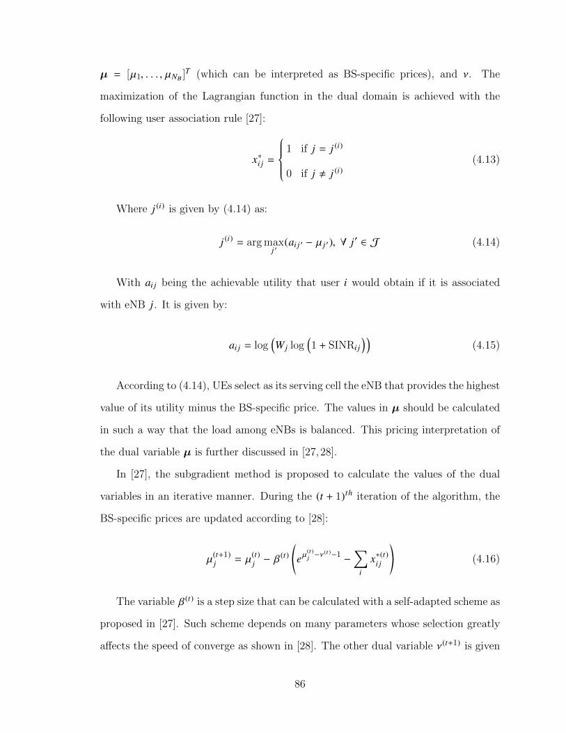
µ = [µ1, . . . , µNB ]T (which can be interpreted as BS-specific prices), and ν. The

maximization of the Lagrangian function in the dual domain is achieved with the

following user association rule [27]:

x∗i j =

1 if j = j (i)

0 if j , j (i)(4.13)

Where j (i) is given by (4.14) as:

j (i) = arg maxj ′

(ai j ′ − µ j ′), ∀ j′ ∈ J (4.14)

With ai j being the achievable utility that user i would obtain if it is associated

with eNB j. It is given by:

ai j = log(W j log

(1 + SINRi j

))(4.15)

According to (4.14), UEs select as its serving cell the eNB that provides the highest

value of its utility minus the BS-specific price. The values in µ should be calculated

in such a way that the load among eNBs is balanced. This pricing interpretation of

the dual variable µ is further discussed in [27,28].

In [27], the subgradient method is proposed to calculate the values of the dual

variables in an iterative manner. During the (t + 1)th iteration of the algorithm, the

BS-specific prices are updated according to [28]:

µ(t+1)j = µ(t)

j − β(t) *

,eµ

(t)j −ν

(t)−1−

∑i

x∗(t)i j+-

(4.16)

The variable β(t) is a step size that can be calculated with a self-adapted scheme as

proposed in [27]. Such scheme depends on many parameters whose selection greatly

affects the speed of converge as shown in [28]. The other dual variable ν(t+1) is given

86

by:

ν(t+1) = log *.,

∑j eµ

(t)j −1

NU

+/-

(4.17)

For the algorithm to converge, all BS-specific prices µ j have to be calculated with

the same value of the step size, hence tight synchronization between eNBs is needed.

Finally, the primal variable X is obtained from the dual variables by applying (4.14).

This load balancing method is summarized in Algorithm 4.2. For a more detailed

description of this method we refer the reader to [27].

Algorithm 4.2 Subgradient method

Initialization: Set µ j = 0,∀ j. Set ν = log∑

j eµ j−1/NU

1: repeat2: UEs are associated to eNBs according to (4.14)3: for each j ∈ J do4: Update BS-specific price µ j with (4.16)5: end for6: eNBs broadcast updated price to all eNBs and users7: Update dual variable ν with (4.17)8: until Dual objective function converges9: Final BS association is given by applying (4.14)

4.4.3 Algorithm based on Dual Coordinate Descend (DCD)

Similarly as in [27], authors in [28] also apply a Lagrangian dual analysis to obtain the

network-wide user association that approximates the solution to (4.9). However, the

use of a dual coordinate descend approach is proposed as the mechanism to update

the BS-specific prices µ j . The values of the BS-specific prices are updated according

to [28]:

µ(t+1)j = sup

{µ j | f (t)

2 (µ j ) − f (t)1 ≤ 0

}(4.18)

With f (t)1 being the number of UEs currently associated to eNB j and f (t)

2 =

eµ(t)j −ν

(t)−1.

87

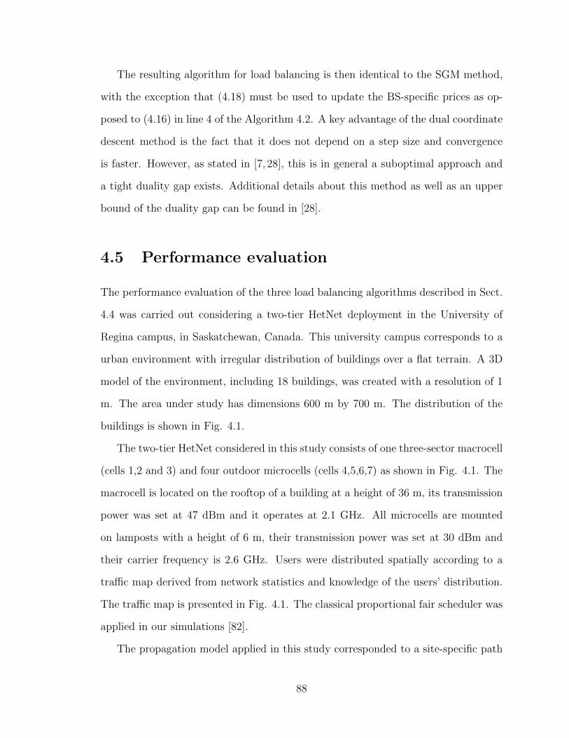
The resulting algorithm for load balancing is then identical to the SGM method,

with the exception that (4.18) must be used to update the BS-specific prices as op-

posed to (4.16) in line 4 of the Algorithm 4.2. A key advantage of the dual coordinate

descent method is the fact that it does not depend on a step size and convergence

is faster. However, as stated in [7, 28], this is in general a suboptimal approach and

a tight duality gap exists. Additional details about this method as well as an upper

bound of the duality gap can be found in [28].

4.5 Performance evaluation

The performance evaluation of the three load balancing algorithms described in Sect.

4.4 was carried out considering a two-tier HetNet deployment in the University of

Regina campus, in Saskatchewan, Canada. This university campus corresponds to a

urban environment with irregular distribution of buildings over a flat terrain. A 3D

model of the environment, including 18 buildings, was created with a resolution of 1

m. The area under study has dimensions 600 m by 700 m. The distribution of the

buildings is shown in Fig. 4.1.

The two-tier HetNet considered in this study consists of one three-sector macrocell

(cells 1,2 and 3) and four outdoor microcells (cells 4,5,6,7) as shown in Fig. 4.1. The

macrocell is located on the rooftop of a building at a height of 36 m, its transmission

power was set at 47 dBm and it operates at 2.1 GHz. All microcells are mounted

on lamposts with a height of 6 m, their transmission power was set at 30 dBm and

their carrier frequency is 2.6 GHz. Users were distributed spatially according to a

traffic map derived from network statistics and knowledge of the users’ distribution.

The traffic map is presented in Fig. 4.1. The classical proportional fair scheduler was

applied in our simulations [82].

The propagation model applied in this study corresponded to a site-specific path

88

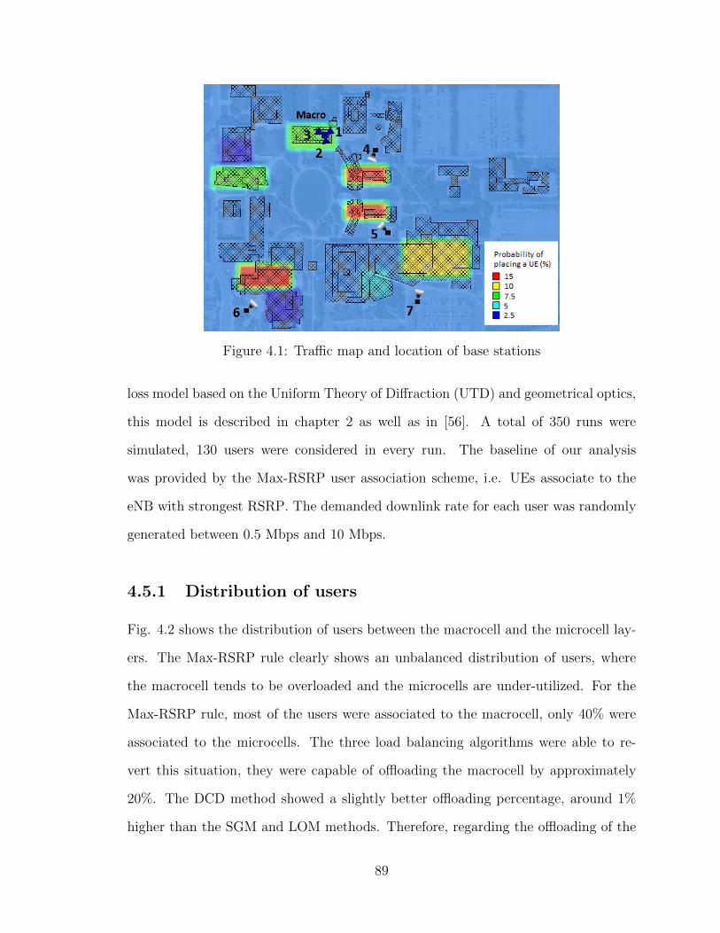
Figure 4.1: Traffic map and location of base stations

loss model based on the Uniform Theory of Diffraction (UTD) and geometrical optics,

this model is described in chapter 2 as well as in [56]. A total of 350 runs were

simulated, 130 users were considered in every run. The baseline of our analysis

was provided by the Max-RSRP user association scheme, i.e. UEs associate to the

eNB with strongest RSRP. The demanded downlink rate for each user was randomly

generated between 0.5 Mbps and 10 Mbps.

4.5.1 Distribution of users

Fig. 4.2 shows the distribution of users between the macrocell and the microcell lay-

ers. The Max-RSRP rule clearly shows an unbalanced distribution of users, where

the macrocell tends to be overloaded and the microcells are under-utilized. For the

Max-RSRP rule, most of the users were associated to the macrocell, only 40% were

associated to the microcells. The three load balancing algorithms were able to re-

vert this situation, they were capable of offloading the macrocell by approximately

20%. The DCD method showed a slightly better offloading percentage, around 1%

higher than the SGM and LOM methods. Therefore, regarding the offloading of the

89

0

10

20

30

40

50

60

70

80

Max-RSRP SGM DCD LOM

Pe

rce

nta

ge

of

use

rs

Macro Micro

Figure 4.2: Distribution of users between macrocell and microcell layers

macrocell, all three load balancing algorithms perform equally good.

4.5.2 Distribution of the load among eNBs

The distribution of users per layer in a HetNet is not enough to measure the effective-

ness of the load distribution among eNBs, especially in the case where the demand of

all users is not assumed constant. It is important to quantify how fair is the sharing

of the load between base stations. This can be done with the calculation of the Jain’s

fairness index F (L). Where L = [LD1 , . . . , LD

NB]T is a vector containing the load indexes

of the NB base stations in the network. The fairness index is calculated according to:

F (L) =

(∑j∈J LD

j

)2NB ·

∑j∈J

(LD

j

)2 (4.19)

The fairness index F (L) takes the maximum value of 1, under the idealistic situation

where the total load is equally shared by all base stations.

Fig. 4.3 shows the results. The Max-RSRP rule showed the lowest value of the

fairness index, reaching only 0.6, this indicates a poor distribution of the load. On the

other hand, the load balancing algorithms achieved a fairer load sharing among base

stations since the value of the fairness index was increased above 0.8. In particular,

90

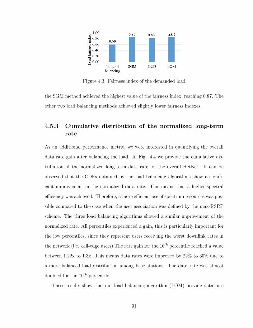
Figure 4.3: Fairness index of the demanded load

the SGM method achieved the highest value of the fairness index, reaching 0.87. The

other two load balancing methods achieved slightly lower fairness indexes.

4.5.3 Cumulative distribution of the normalized long-termrate

As an additional performance metric, we were interested in quantifying the overall

data rate gain after balancing the load. In Fig. 4.4 we provide the cumulative dis-

tribution of the normalized long-term data rate for the overall HetNet. It can be

observed that the CDFs obtained by the load balancing algorithms show a signifi-

cant improvement in the normalized data rate. This means that a higher spectral

efficiency was achieved. Therefore, a more efficient use of spectrum resources was pos-

sible compared to the case when the user association was defined by the max-RSRP

scheme. The three load balancing algorithms showed a similar improvement of the

normalized rate. All percentiles experienced a gain, this is particularly important for

the low percentiles, since they represent users receiving the worst downlink rates in

the network (i.e. cell-edge users).The rate gain for the 10th percentile reached a value

between 1.22x to 1.3x. This means data rates were improved by 22% to 30% due to

a more balanced load distribution among base stations. The data rate was almost

doubled for the 70th percentile.

These results show that our load balancing algorithm (LOM) provide data rate

91

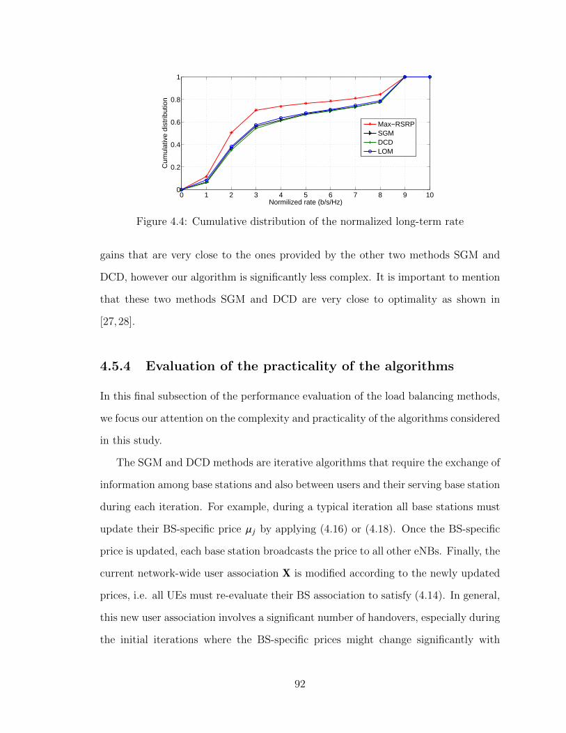
0 1 2 3 4 5 6 7 8 9 100

0.2

0.4

0.6

0.8

1

Normilized rate (b/s/Hz)

Cum

ulat

ive

dist

ribut

ion

Max−RSRPSGMDCDLOM

Figure 4.4: Cumulative distribution of the normalized long-term rate

gains that are very close to the ones provided by the other two methods SGM and

DCD, however our algorithm is significantly less complex. It is important to mention

that these two methods SGM and DCD are very close to optimality as shown in

[27,28].

4.5.4 Evaluation of the practicality of the algorithms

In this final subsection of the performance evaluation of the load balancing methods,

we focus our attention on the complexity and practicality of the algorithms considered

in this study.

The SGM and DCD methods are iterative algorithms that require the exchange of

information among base stations and also between users and their serving base station

during each iteration. For example, during a typical iteration all base stations must

update their BS-specific price µ j by applying (4.16) or (4.18). Once the BS-specific

price is updated, each base station broadcasts the price to all other eNBs. Finally, the

current network-wide user association X is modified according to the newly updated

prices, i.e. all UEs must re-evaluate their BS association to satisfy (4.14). In general,

this new user association involves a significant number of handovers, especially during

the initial iterations where the BS-specific prices might change significantly with

92

respect to the previous iteration.

The SGM and DCD methods require the exchange of at least m(NB+NU ) messages

where m is the number of iterations [27]. On the other hand, our load balancing

algorithm only requires each base station to broadcast its demanded load index. An

overloaded base station would proceed to execute Algorithm 4.1 and select the UEs

that would be transfered to lightly loaded base stations (i.e. set Tj), at this point only

UEs currently associated with overloaded base stations would be handed over, there

is no need to update the network-wide user association as it is done in every iteration

of the SGM and DCD methods. Therefore, our load balance algorithm requires the

exchange of NB +∑

j∈J |Tj | messages.

Fig. 4.5 shows the average number of additional exchanged messages due to

the application of the load balancing algorithms. The SGM method requires an

extraordinary amount of exchanged messages due to the fact that its convergence

is slow, as opposed to the DCD method. Our load balancing algorithm requires

a small amount of exchange of messages among base stations, this leads to lower

levels of required coordination and lower impact on the signaling load of the network.

Furthermore, our algorithm would have a reduced impact on power consumption

as opposed to the DCD and SGM methods. Therefore, it is evident that in terms

of practicality as well as impact on power consumption, our algorithm is superior.

Additionally, with a lower number of triggered handovers the effects on user experience

are reduced.

4.6 Summary

In this chapter, we propose a novel and practical load balancing algorithm based

on local maximization of the sum of the utilities. Furthermore, we carried out the

evaluation of the performance of our load balancing algorithm through a comparative

93

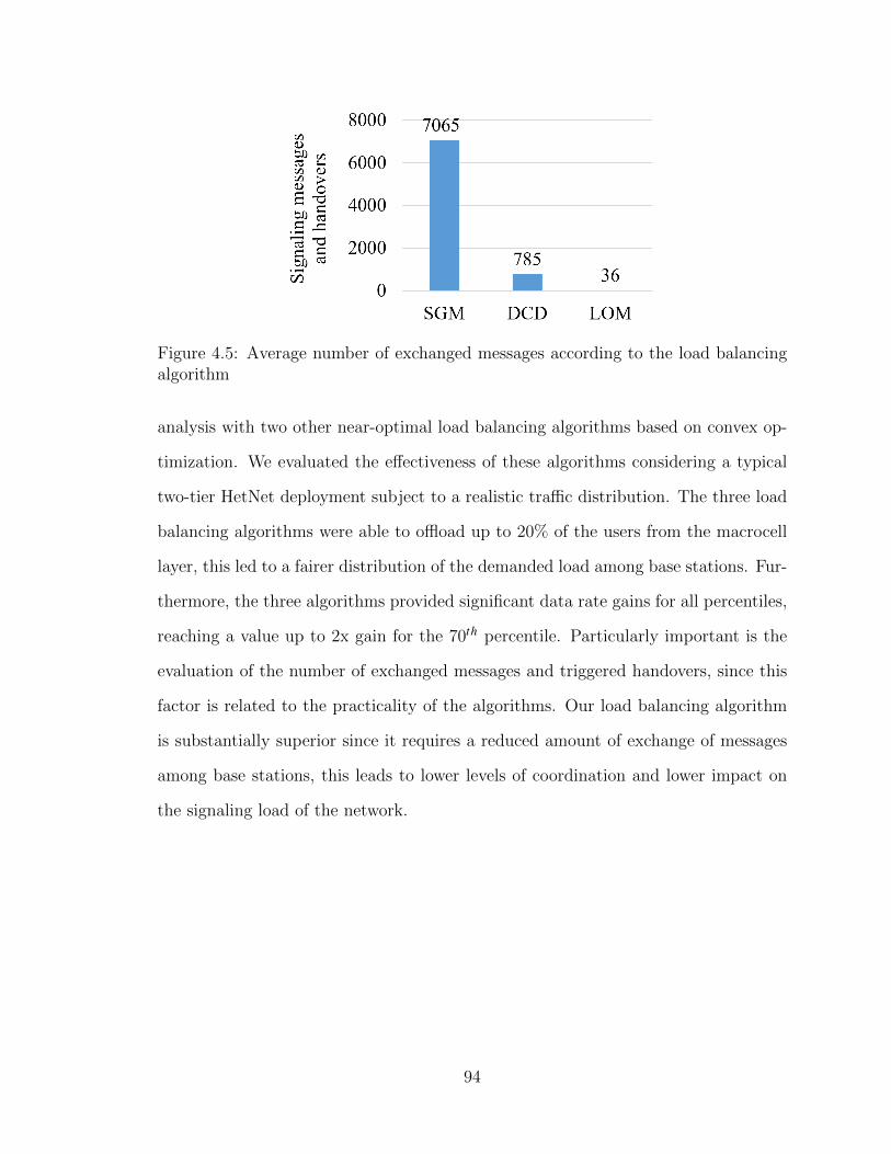
Figure 4.5: Average number of exchanged messages according to the load balancingalgorithm

analysis with two other near-optimal load balancing algorithms based on convex op-

timization. We evaluated the effectiveness of these algorithms considering a typical

two-tier HetNet deployment subject to a realistic traffic distribution. The three load

balancing algorithms were able to offload up to 20% of the users from the macrocell

layer, this led to a fairer distribution of the demanded load among base stations. Fur-

thermore, the three algorithms provided significant data rate gains for all percentiles,

reaching a value up to 2x gain for the 70th percentile. Particularly important is the

evaluation of the number of exchanged messages and triggered handovers, since this

factor is related to the practicality of the algorithms. Our load balancing algorithm

is substantially superior since it requires a reduced amount of exchange of messages

among base stations, this leads to lower levels of coordination and lower impact on

the signaling load of the network.

94

Chapter 5

Classification of user trajectories inHetNets using

unsupervised-shapelets andmulti-resolution wavelet

decomposition

The classification of user trajectories in heterogeneous networks is investigated in

this chapter. We propose a methodology to classify users trajectories based on the

measurement reports submitted to the serving base station as part of the handover

process, we propose to consider each measurement report as a time series. This

methodology allows base stations to automatically and autonomously discover the

RF conditions of their cell-edge (e.g. signal strength degradation and interference

levels). We propose the application of machine learning and data mining techniques

to identify patterns in the RSRP measurement reports submitted by users as they

approach the edge of the service area. Our time series clustering algorithm based on

unsupervised-shapelets and multi-resolution wavelet decomposition provided superior

performance compared to a DFT-based clustering algorithm. Our algorithm was able

to provide clustering results with an average accuracy of 95%. Furthermore, the

quality measure of the resulting clusters was up to 75% better compared to the

clustering results provided by the DFT-based algorithm. We also proposed a novel

methodology to calculate a suitable number of clusters without any prior knowledge

regarding the data, an average accuracy close to 90% was achieved.

95

5.1 Introduction

HetNets are particularly useful and a cost-effective solution to provide high quality

service to traffic hotspots. However, the optimization of handover parameters in

HetNets is a challenging task for network operators, due to the combination of low

power and high power base stations. It is essential for operators to properly set up

mobility management parameters to guarantee the continuity of service as users move

between coverage areas.

The handover (HO) procedure is controlled by a set of multiple parameters, whose

optimization is highly dependent on the RF conditions at the cell-edge. In certain

situations, it might be preferred to execute an HO faster due to rapidly degrading

RF conditions as users approach the cell-edge in order to avoid a radio link failure.

In other situations, it might be better to delay the execution of the HO to avoid

unnecessary handovers due to a fluctuation of the signal from the base station (eNB)

during a short period. Therefore, the conditions of the cell-edge (e.g. signal strength,

interference level) and user behavior (e.g. user speed) determine the proper set of

HO parameters for optimal operation.

Determining the RF conditions at the cell-edge is challenging in HetNets, since

the geographical location of users is usually not available in LTE systems. Therefore,

base stations do not know precisely where their users are located or the direction of

their movement, particularly in indoor environments.

In this study, we propose the use of Reference Signal Received Power (RSRP)

measurements reported by users to identify archetypal movements of mobiles as they

leave the service area of a small cell in an indoor environment. This identification is

carried out by the application of machine learning and data mining techniques.

Consider a picocell system providing service in a food court area of a university

campus, the movement of users entering and leaving the building is somewhat pre-

96

defined, in the sense that people walk along hallways and leave the building through

doors whose positions remain unchanged. Therefore, users following similar trajecto-

ries will report RSRP measurements that are highly correlated, and this information

can be used to identify the RF propagation conditions that those users are subject to

as they move. Furthermore, this information can be used to predict the RF propaga-

tion conditions that future users, which will also follow those archetypal trajectories,

will be subject to as well.

We have identified three main areas where the classification of user trajectories in

HetNets can provide essential benefits: 1) cell-edge characterization, 2) Mobility Ro-

bustness Optimization (MRO) in the context of self-optimizing networks (SON) and

3) load balancing. We briefly describe these applications in the following subsections.

5.1.1 Cell-edge characterization

In order to increase the capacity of their macro-only network, many operators deploy

small cells to provide service to traffic hotspots located indoors. In such scenario,

the area surrounding the building is typically serviced by high power macrocells.

Therefore, the cell-edge of the small cells tend to be subject to different interference

levels according to the relative location of the macrocell tower with respect to the

building [46]. The signal of the macrocell might be stronger in certain areas of the

buildings. This essentially leads to uneven interference levels at the cell-edge of the

small cells. This situation makes the tuning of HO parameters (e.g. time-to-trigger)

very challenging. If one unique set of HO parameters is applied, then these param-

eters could be too conservative for those cell-edge users subject to higher levels of

interference (leading to too late HOs) or too aggressive for those suffering lower levels

of interference (leading to ping-pong events). The identification of the RF propaga-

tion conditions at the cell-edge of small cells, can provide the necessary information

97

to optimally tune the HO parameters.

5.1.2 Mobility robustness optimization in SON

In the context of SON, the MRO function is intended to automate the adjustment of

HO parameters based on current loading conditions and the presence of neighboring

cells. It is expected that in the coming years, operators will have to increase the

densification of their small cell deployments in order to keep up with service demand.

This is especially relevant in indoor environments where picocells and even micro-

cells are being largely deployed nowadays, and it could be cumbersome for operators

to manually deal with the setting of HO parameters every time a new small cell is

installed. With the MRO functionality, the optimization of HO parameters should oc-

cur automatically. Therefore, if base stations are able to determine the RF conditions

of their cell-edges on a cell-pair basis, they will be able to autonomously cooperate

and define the best set of HO parameters that guarantee continuity of service as users

move between coverage areas.

5.1.3 Load balancing optimization

HetNets are deployed to offload the already congested macrocells, therefore it is es-

sential to properly balance the load between tiers in a HetNet system. If base stations

are able to predict when users are about to approach their cell-edge and enter the

service area of a neighboring cell, then they can use this information to either delay

the execution of an HO or execute it earlier according to a load balancing criteria,

that considers the loading conditions of the serving and neighboring cells. In some

instances, a mobile user (UE) might receive better service if it stays connected to a

lightly loaded cell that is not necessarily its best server from a RSRP point of view.

This idea has been explored by Sas et al. in [55],where they apply machine learning

98

techniques to improve traffic steering between neighboring cells.

The rest of the chapter is organized as follows: in Sect. 5.2 a brief description of

the current work in this area is provided. In Sect. 5.3 we describe the contributions of

this chapter. In Sect. 5.4 we briefly describe the handover process and the collection

of measurement reports. In Sect. 5.5 we provide details regarding the clustering of

time series and we describe our clustering algorithm. The performance evaluation of

our approach is presented in Sect. 5.6 and we provide a summary in Sect. 5.7.

5.2 Related work

Sas et al. proposed the classification of users based on their mobility behavior in [55].

They proposed the collection of RSRP measurement reports submitted by a limited

set of users, labeled as “reference users”, as they move along the service area of a

homogeneous network with multiple macrocells. Their objective was to match the

RSRP measurement reports from new users to those reports previously collected from

the reference users. The matching is carried out by applying a modified version of

the well-known Dynamic Time Warping (DTW) algorithm. If a user is matched to

one of the reference reports, then it is assumed that this user will follow the same

trajectory as the matched reference user. To the best of our knowledge, this is the

only attempt to identify user trajectories based on measurement reports currently in

the literature.

Our approach is much more comprehensive in the sense that, without any prior

knowledge on the number of possible user trajectories, we propose the use of a clus-

tering algorithm to identify typical user movements, instead of just selecting as a

reference the measurement reports from a single user as it is done in [55]. We ap-

ply machine learning and data mining techniques to automatically identify patterns

99

in the measurement reports submitted by multiple users. We use such patterns to

cluster the measurement reports and identify the RF propagation conditions that

users, following such archetypal trajectories, are subject to. The authors in [55] only

treated the problem of matching measurement reports to a reference. Furthermore,

we extend this idea to the case of heterogeneous networks, in particular small cells

providing coverage in indoor environments.

5.3 Contributions

The contributions of the work described in this chapter can be summarized in three

main points:

1. Our approach is intended to provide base stations with a mean to automatically

and autonomously discover the RF conditions (e.g. signal levels and interfer-

ence) that their users are subject to as they move through the cell-edge. For

this purpose we propose the use of machine learning and data mining techniques

to identify such patterns in the RSRP measurement reports submitted by users

as part of the handover process.

2. We propose a novel time series clustering algorithm based on shape similarity

to identify and classify such patterns. We propose to apply a shape-based tech-

nique called unsupervised-shapelets combined with a multi-resolution wavelet

decomposition analysis.

3. We propose a novel methodology to automatically determine a suitable number

of clusters without any prior knowledge about the data being classified. This

will allow base stations to identify any number of patterns in the measurement

reports submitted by users without any previous knowledge. This is a relevant

contribution due to the fact that the identified patterns can change with time

100

as the conditions of the network change (e.g. a new small cell is deployed

nearby). Therefore, the base station can automatically discover the number of

new patterns subject to the changing network conditions.

5.4 Handovers and RSRP measurement reports in

LTE/LTE-A systems

In this study we focused on the hard handover process in 3GPP LTE/LTE-A systems

for UEs in connected state (i.e. mobiles actively receiving and sending data to their

serving eNB). The handover procedure consists of four main phases [83]: measure-

ment, processing, preparation, and execution. UEs continuously monitor the received

signal strength from their serving eNB (SeNB) and the RSRP from their neighboring

cells. This is typically carried out by measuring the RSRP levels (UEs can also mon-

itor the signal quality in terms of the Reference Signal Received Quality - RSRQ).

The measurements values gathered by the UEs are further processed to remove the

effects of fading, this is done by averaging and filtering the measurements at two

different layers L1 (physical) and L3 (network). At the L1 layer, the UE collects

several RSRP values during an interval period defined by the network operator (e.g.

one sample every 40 ms during a period of 200 ms) and an L1 sample is generated

by linearly averaging the collected RSRP values. At the L3 layer, the L1 samples are

then averaged through a first-order infinite impulse response (IIR) filter according to

(5.1), a process known as L3-filtering.

Fn = (1 − a)Fn−1 + aMn (5.1)

Where Mn is the latest L1 sample, Fn is the updated filtered L3 sample, Fn−1 is

the previous filtered L3 sample and a is defined as [83]:

a =1

2k/4 (5.2)

101

Where k is known as the L3-filter coefficient and it is set by the network operator.

We will refer to the L3 samples simply as RSRP samples. UEs send measurement

reports to their SeNB whenever certain conditions regarding the RSRP samples occur.

These conditions, or events, are standardized and set up by the network operator.

There are several events that can trigger the report of RSRP measurements, named

events A1 through A6. A detailed description of these events can be found in [83]. In

our study we focused on the A2 event for intra-carrier HOs. The entry condition for

the A2 event occurs when the RSRP samples of the SeNB becomes worst than certain

threshold (A2 threshold). A hysteresis parameter is also applied to avoid unnecessary

triggering of the event due to rapid fluctuations of the RSRP samples. Once the entry

condition is satisfied, it has to remain valid for a certain period before the UE submits

the measurement report to the SeNB. This period is called time-to-trigger (TTT) and

it can take values from 40 ms up to 5120 ms. The A2 threshold, hysteresis, TTT and

L3-filter coefficient k are fundamental parameters that control the HO process. These

parameters need to be optimized by network operators for specific network conditions

in order to guarantee the continuity of service as users move between coverage areas

(i.e. to reduce HO failures).

HO failures typically occur when the HO event is executed too late (i.e. a radio

link failure occurs before the HO is completed). A reduction of the TTT helps reduce

too late HO failures since the HO is executed faster. However, a small TTT increases

the chances of ping-pong events (i.e. UE is handed over back and forth from SeNB

and the target eNB over a short period), this is undesirable since it increases the

signaling load in the network due to unnecessary HO operations. HO parameters

can also be setup at the cell-pair level, this is especially useful in HetNets since the

cell-edge conditions for small cells are highly irregular, as pointed out in Sect. 5.1,

and a single set of HO parameters for all cells might not provide optimal results.

In this study, we consider the set of RSRP samples submitted to the SeNB (i.e.

102

the measurement report) as a time series that can be used to identify archetypal

movements of users in indoor environments. As pointed out in [55], users that move

along similar trajectories will provide measurement reports that are highly correlated

with each other. Therefore, we propose to automatically identify patterns that will

allow the base station to determine the typical RF conditions as users approach the

cell-edge. In order to identify such patterns, we propose the use of machine learning

and data mining techniques, this includes the clustering of a collection of time series.

Details regarding time series and their clustering are provided in the next section.

5.5 Clustering of time series

A time series is an ordered sequence of real-valued data, usually recorded at regular

time intervals. We define a time series of length m as Ti = Ti1,Ti2, . . . ,Tim. A collection

of N time series is defined as the set T = {T1,T2, . . . ,TN }, the time series in T need not

have the same length. Each time series Ti is associated with a class (or cluster) label,

the time series sharing similar features or attributes form a class, i.e. are associated

with the same class label. The problem of clustering the time series in T consists

of finding a function that maps from the space of time series to the space of class

values [86].

A similarity measure is required in order to classify a set of time series T, a suitable

similarity measure is able to effectively discriminate among time series and facilitates

the classification. In some cases, similarity in time is suitable to classify the data,

while other problems require a similarity measure based on shape. Therefore, the

selection of the similarity measure depends on the domain of the problem at hand.

In our study, each time series is a collection of RSRP measurements gathered by a

single UE in connected mode. Our premise is that those users moving along similar

trajectories, at approximately the same speed, should generate time series with similar

103

shape. Hence, we focused on studying the clustering of time series with a shape-based

similarity measure.

Shaped-based similarity measures determine the level of similarity between two

time series by comparing their individual values. The most popular examples of this

type of measure are the Euclidean distance and Dynamic Time Warping (DTW) [87].

The Euclidean distance has become widely used in data mining applications not

only due to its simplicity, but also because experimental evaluations have proven its

accuracy as a similarity measure [88]. The Euclidean distance between two series Ti

and Tj with equal length m, is given by:

D(Ti,Tj ) =

√√ m∑k=1

(Tik − Tj k

)2(5.3)

The lower the value of D(Ti,Tj ), the more similar the two time series. Note that for

the Euclidean distance to be invariant to scale, the time series need to be z-normalized

first (i.e. both time series must have zero mean and unit variance). The Euclidean

distance can only be applied to compare two time series with the same length and

time alignment. DTW was proposed as an alternative method to compare time series

with different time lengths and not aligned in time [55], with the disadvantage of

being a computationally expensive method.

In our study, we propose the use of the time series obtained from the measurement

of RSRP values to identify typical trajectories (or archetypal movements) of users in

indoor environments, e.g. users moving along a hallway and leaving the building at a

particular exit. Multiple users, moving along similar trajectories, will generate similar

time series that belong to the same class.

The main challenge is to effectively cluster such set of time series with no prior

knowledge regarding the number of classes. Furthermore, the time series to be clus-

tered do not have the same length in general. Therefore, the simple application of

the Euclidean distance to classify T is not suitable for our application and a more

104

sophisticated technique is required.

Our objective is to exploit local similarities in shape among time series, e.g. a

sharp drop in RSRP values due to the presence of a concrete wall as users leave the

service area of an in-building system. Such drop in RSRP values should be highly

correlated among users walking along the same path. This type of local similarity

in shape can provide the necessary information to classify the time series. For this

reason, we apply a technique called shapelets, proposed originally by Ye and Keogh in

[89]. Shapelets are specifically intended to identify local shape features (i.e. patterns)

that contain enough information to discriminate among time series. In the next

section we briefly provide details about the definition of shapelets and their use for

clustering of time series.

5.5.1 Shapelets

A shapelet is defined as a subsequence of one time series in T [86]. A subsequence

s of length l is defined as a subset of l consecutive values from a time series. A

shapelet is selected in such a way that it captures a distinctive shape feature that is

common in a class of time series. Shapelets can be found via exhaustive search, where

every possible subsequence of each time series in T is a candidate to be selected as a

shapelet [89]. However, this process is time consuming, more efficient techniques for

shapelet generation have been proposed [86,90].

The process of discovering shapelets for clustering of time series involves three

main stages: generation of candidates, measure the similarity between a candidate and

the time series in the set, and finally, the assessment of the quality of the candidate.

Regarding the generation of shapelet candidates, it is necessary to define the length

of the candidate subsequences first. Typically, subsequences with lengths between

predefined values lmin and lmax are considered. If exhaustive search is used to generate

105

shapelet candidates, then all possible subsequences with lengths between lmin and lmax

are extracted from the time series in T. This process is slow and inefficient for large

sets of time series with long lengths. Instead of applying an exhaustive search to

generate shapelets, we apply the algorithm proposed by Zakaria et al. in [90] with

slight variations to accommodate the fact that we deal with time series with different

lengths.

In [90], the authors proposed the use of unsupervised-shapelets to cluster time

series. We briefly describe the algorithm in the next subsection.

5.5.2 Generating unsupervised-shapelets

According to the authors in [90], shapelets can be generated iteratively. In the first

iteration, the algorithm looks for a candidate subsequence s capable of separating the

set of time series T in two distinct subsets, namely DA and DB, such candidate can

be used as a shapelet. The subset DA corresponds to the time series that contain a

similar pattern as the candidate s. The subset DB corresponds to the rest of the time

series which do not contain the pattern. Therefore, in the next iteration, to generate

a shapelet candidate it is only necessary to evaluate subsequences from any of the

time series in DB. With every new generated shapelet, the number of time series in

DB decreases, this avoids the need for an exhaustive search and speeds up the process

of generating shapelets.

In order to evaluate the capacity of a candidate subsequence s to discriminate the

time series in T, a similarity measure between the subsequence s of length l and a

time series T of length m has to be defined first. In [90], this similarity measure is

called subsequence distance sD(s,T ) and it is defined as:

sD(s,T ) = mini∈{1,m−l}

D(s, ti,l ) (5.4)

106

Where ti,l is a subsequence of T that contains l values of T starting from the

ith value, with l < m. According to (5.4), a low sD(s,T ) indicates a high level of

similarity between the time series T and the subsequence s.

As it was pointed out before, a candidate subsequence is selected as a shapelet

based on its discriminative power, which is measured by how much distinct the subsets

DA and DB are. This corresponds to the quality assessment of the candidate shapelet.

To generate the subsets DA and DB, first all distances sD(s,Ti) between a candidate

subsequence s and the time series in T are calculated. This step, maps each time

series in T to the real value obtained with (5.4), i.e. a one dimensional feature space.

The set of the values sD(s,Ti) form a set defined as Dist(s). In [90], a greedy search

algorithm is applied to separate the set of values in Dist(s) in two clusters, i.e. the

subsets DA and DB.

The discriminative power of the candidate subsequence s is determined by how

much apart the elements in DA are from the elements in DB in the feature space.

This is measured by a quantity defined as the gap:

gap = µB − σB −(µA − σA

)(5.5)

Where µB and µA are the mean of the subsequence distances between s and

the time series in DA and DB respectively and, σB and σA are the corresponding

standard deviations. The higher the gap, the higher the discriminative power of the

subsequence s.

In the algorithm proposed in [90], the initial set of candidate subsequences is

generated from time series T1. This means, all subsequences with lengths between

lmin and lmax are extracted from T1 and their associated gap is calculated with (5.5).

Let sh1 be the first shapelet to be selected. The shapelet sh1 corresponds to the

subsequence with the highest quality, i.e. the highest value of the gap. The next set

of candidate subsequences is generated from a time series in the subset DB (where DB

107

which was obtained when sh1 was selected as shapelet), and the process is repeated

to generate the second shapelet. The procedure is repeated until there are no more

time series in the corresponding subset DB.

We refer the reader to [90] for additional details of the algorithm to generate

unsupervised-shapelets.

5.5.3 Clustering using unsupervised-shapelets

After generating a set of shapelets, the next step is to use them to cluster all the time

series in T. This is done by creating a new feature space with the so-called shapelet

transformation [86].

The shapelet transformation consists in mapping every time series Ti ∈ T to a

n-dimensional vector, known as the feature vector. Where n is the number of gener-

ated shapelets and every entry of the feature vector corresponds to the subsequence

distance between the time series Ti and each shapelet. Consider the set S containing

the n generated shapelets, i.e. S = {sh1, sh2, . . . , shn}, the feature vector fi associated

with time series Ti, is given by:

fi = [sD(sh1,Ti), sD(sh2,Ti), . . . , sD(shn,Ti)] (5.6)

With (5.6), each one of the N time series in T is mapped to a feature vector.

The collection of the N feature vectors can now be used as the input to a clustering

algorithm. In our study we applied the popular K-means algorithm. This algorithm

was proposed in 1967 by McQueen in [91] and due to its simplicity it has become one

of the most popular clustering algorithms in the data mining community.

The K-means algorithm classifies the feature vectors in the n-dimensional space

into K different clusters, where the number of clusters is known a priori. The algo-

rithm consists of four main steps:

108

1. Define the position of K points in the n-dimensional space, these points will serve

as the centroids of the K clusters (random positions are typically selected)

2. Assign each feature vector to the centroid with smallest Euclidean distance

3. Recalculate the centroids of each cluster based on the assignment done in step

2.

4. Repeat steps 2 and 3 until the centroids do not change

Notice that the K-means algorithm requires the number of clusters to be known a

priori. In our application, the base stations do not know how many different archety-

pal trajectories can be identified a priori. To overcome this situation, we have devel-

oped a methodology to automatically determine the number of clusters without prior

knowledge. This methodology in described in Sect. 5.5.6.

5.5.4 Wavelets and multi-resolution analysis

In our study, we consider time series that are generated by the RSRP measurement re-

ports submitted by UEs to their serving base station. The RSRP measurement values

typically change abruptly over short periods, this is due to the rapidly changing prop-

agation conditions of reference signals as the mobiles move along certain trajectory.

Furthermore, RSRP measurements are usually subject to noise that makes even more

difficult the clustering of the resulting time series, in particular when shape-based

similarity measures are applied, e.g. shapelets.

In order to improve the robustness and accuracy of the clustering method de-

scribed in Sect. 5.5.3, we propose the combination of a multi-resolution wavelet de-

composition analysis with the unsupervised-shapelets technique. Most of the abrupt

variations in RSRP measurements as well as the noise present in the measurements

109

are captured by a high resolution approximation of the time series, whereas its fun-

damental shape is captured by a low resolution approximation. The application of

multi-resolution wavelet decomposition allow us to perform the clustering of time se-

ries starting from low resolution levels (coarse approximation of the data), where most

of the noise and abrupt changes in RSRP measurements do not significantly alter the

shape of the time series, and we incrementally increase the resolution of the approxi-

mation of the time series to refine the output of the clustering algorithm. To the best

of our knowledge, this is the first time that shapelets and wavelet decomposition are

combined for the clustering of time series.

Multi-resolution wavelet analysis has been widely applied for image compression

and other signal processing techniques [92]. More recently, wavelet-based clustering

algorithms have also been proposed [93]. Wavelets are mathematical functions used

to represent data or other functions at different levels of resolution [92]. The discrete

wavelet analysis procedure consists of selecting a prototype function, also known as

the mother wavelet, and expressing the data of interest in terms of averages and

differences of the mother wavelet. Since wavelets are localized in time, they are

capable of capturing levels of details from the data at different scales of resolution.

This represents an advantage compared to Fourier analysis that is only able to capture

global characteristics of the data.

In our study, we propose the use of the Haar wavelet decomposition to extract the

representation of time series with different resolution levels. Consider a time series

T , the first level of the decomposition is obtained by averaging every two adjacent

values of T . As a result, a smoother representation of T is obtained. If the length of

T is m = 2p, the length of the first decomposition of T is 2p−1.

The Haar wavelet has very important properties that makes it suitable for our

application. For example, it is simple and easy to compute, its computation requires

linear time in the length of the sequence [94]. Furthermore, it preserves the Euclidean

110

distance, as it was shown in [94] and the decomposition via the Haar wavelet allows

for perfect reconstruction.

In the next subsection we provide a description of our algorithm for clustering of

time series based on multi-resolution analysis and unsupervised-shapelets.

5.5.5 Clustering of time series with multi-resolution analysisand shapelets

Our algorithm to cluster time series is based on the principle that the clustering is

more robust when it is done iteratively starting with a low resolution approximation

of the time series and refining the clusters by considering a finer approximation of

the data in every iteration. The multi-resolution wavelet decomposition of the data

provides approximations of the time series with different levels of detail. A similar

approach was followed in [93] for an “anytime clustering algorithm” based on K-

means.

Our algorithm starts with the computation of the Haar wavelet decomposition

of all the time series in T. During the first iteration of the algorithm, the low-

est resolution approximation of each time series is considered as the input of the

unsupervised-shapelet generation algorithm described in Sect. 5.5.2. As a result, this

set of shapelets is used to cluster the lowest resolution approximation of the time se-

ries in T using the K-means algorithm. During the first iteration, the position of the

cluster centroids in the feature space are selected randomly (first step of the K-means

algorithm as described in Sect. 5.5.3).

In the second iteration, the algorithm tries to refine the clustering of time series

by considering the wavelet decomposition of the time series with the next level of

resolution. These approximations of the time series are used as the input of the

unsupervised-shapelet generation algorithm. The new set of shapelets is then used

to cluster this higher resolution representations of the time series. For the second

111

Table 5.1: Calculation of Rand index

Quantity DescriptionA number of instances in same class in Cls1 and Cls2B number of instances in different clusters in Cls1 and Cls2C number of instances in same cluster in Cls1 but not on Cls2D number of instances in same cluster in Cls2 but not on Cls1

iteration, the K-means algorithm is not initialized randomly. Instead, we use the

cluster memberships from the previous iteration to calculate the initial position of

the cluster centroids.

The resulting clusters from the previous resolution level are compared with the

clusters obtained with the higher resolution level. If the memberships of the clusters

did not change, then the algorithm stops. Otherwise, the resolution level is increased

by one level and the process is repeated. We compared the clustering results ob-

tained with two different levels of resolution by applying the well-known Rand index,

typically used as a clustering quality measure.

The Rand index RI is a number in the interval [0, 1] and it measures the similarity

between two clusterings Cls1 and Cls2. To compute the RI index, it is necessary first

to compute the quantities described in table 5.1, then the Rand index is calculated

with (5.7).

RI (Cls1,Cls2) =A + B

A + B + C + D(5.7)

The Rand index takes the value of 0 if the clusterings Cls1 and Cls2 are completely

different. It takes the value of 1, when both clusterings are identical (i.e. quantities

C and D from table 5.1 are zero).

The algorithm to cluster time series is summarized in Algorithm 5.1.

Noticed that in line 4 of Algorithm 5.1, the function

GetClusters(Data leveli, Si,Clsi−1) is executed to cluster the data’s ith level of

resolution with the corresponding set of shapelets Si and initializing the K-means

112

Algorithm 5.1 Algorithm to cluster time series based on multi-resolution analysisand shapelets

Require: Set of time series T, max. wavelet decomposition level levelmax1: for i = 1 to levelmax do2: Data leveli ← Haar (T, i)3: Si ← GenShapelets(Data leveli)4: Clsi ← GetClusters(Data leveli, Si,Clsi−1)5: if i > 1 then6: RI ← Rand Index(Clsi−1,Clsi)7: if RI = 1 then8: Return Clsi9: end if

10: end if11: end for

algorithm with the centroids from the clusters obtained in the previous iteration.

This function implements the K-means algorithm combined with our methodology

to automatically determine the number of clusters in the data. We proceed to briefly

describe this methodology in the next subsection.

5.5.6 Automatic determination of the number of clusters

Our algorithm to cluster time series is based on the popular K-means algorithm

described in Sect. 5.5.3. This algorithm requires the number of clusters K to be

known a priori. In our study, the number of clusters corresponds to the number

of different trajectories that can be identified from the RSRP measurement reports

submitted by users. We do not assume that base stations know this number a priori,

therefore we propose an algorithm to automatically determine a suitable value for K .

Typically, in data mining applications if the number of clusters is not known a

priori then a trial-and-error procedure is followed to determine a suitable number of

clusters. This procedure usually requires a subjective evaluation of the clustering

results [95], e.g. visual inspection.

A simple approach to determine the number of clusters K, consists of applying the

113

K-means algorithm for a range of values for K, say between Kmin and Kmax. Then,

apply a quality measure to determine which value of K provided the best clustering

for the data [95]. A typical metric used to measure the quality of a clustering is the

sum of the squared Euclidean distance between each data instance (i.e. each time

series) and the centroid of the cluster it was assigned to, such distance is measured in

the n-dimensional feature space. The sum of the squared Euclidean distances SSE(k)

is calculated as:

SSE(k) =k∑

j=1

Nj∑i=1

(D( fi,w j )

)2(5.8)

Where k is the number of clusters, N j is the number of data instances in the jth

cluster, fi is the feature vector associated with the ith data instance in cluster j and,

w j is the centroid of the jth cluster. If the data were correctly clustered, then it is

expected that each data instance will be located close to the centroid of its cluster

and the value of SSE(k) will be lower, as opposed to the case when the number of

clusters does not suit the data and a high value of SSE(k) is observed.

The SSE(k) metric has its maximum value when k = 1 and decreases as the

number of clusters k is increased, until the point that it takes the value of 0 when

each data instance is a cluster on its own, a situation that is not desirable. However,

the plot of SSE(k) with respect to the number of clusters k has a very characteristic

shape as shown in Fig. 5.1 (note that the SSE(k) has been normalized with respect

to SSE(1)). There is typically a maximum value for k that significantly reduces the

value of SSE(k), increasing k beyond that value does not provide any additional

benefit in the reduction of the SSE. Therefore, a suitable value for K is obtained by

finding the elbow in the curve of the SSE(k) plot. This is a heuristic method known

as the Elbow method [95]. Unfortunately, there is no clear definition for the elbow of

the curve.

A more formal approach was proposed by Pham et al. in [95], where an evalua-

114

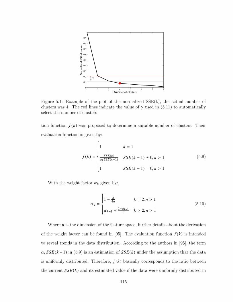
1 2 3 4 5 6 7 80

0.1

0.2

0.3

0.4

0.5

0.6

0.7

0.8

0.9

1

Number of clusters

Nor

mal

ized

SS

E d

ecre

ase

Figure 5.1: Example of the plot of the normalized SSE(k), the actual number ofclusters was 4. The red lines indicate the value of γ used in (5.11) to automaticallyselect the number of clusters

tion function f (k) was proposed to determine a suitable number of clusters. Their

evaluation function is given by:

f (k) =

1 k = 1

SSE(k)αkSSE(k−1) SSE(k − 1) , 0, k > 1

1 SSE(k − 1) = 0, k > 1

(5.9)

With the weight factor αk given by:

αk =

1 − 34n k = 2, n > 1

αk−1 +1−αk−1

6 k > 2, n > 1

(5.10)

Where n is the dimension of the feature space, further details about the derivation

of the weight factor can be found in [95]. The evaluation function f (k) is intended

to reveal trends in the data distribution. According to the authors in [95], the term

αk SSE(k − 1) in (5.9) is an estimation of SSE(k) under the assumption that the data

is uniformly distributed. Therefore, f (k) basically corresponds to the ratio between

the current SSE(k) and its estimated value if the data were uniformly distributed in

115

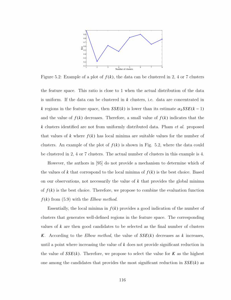
1 2 3 4 5 6 7 80.1

0.2

0.3

0.4

0.5

0.6

0.7

0.8

0.9

1

Number of clusters

f(k)

Figure 5.2: Example of a plot of f (k), the data can be clustered in 2, 4 or 7 clusters

the feature space. This ratio is close to 1 when the actual distribution of the data

is uniform. If the data can be clustered in k clusters, i.e. data are concentrated in

k regions in the feature space, then SSE(k) is lower than its estimate αk SSE(k − 1)

and the value of f (k) decreases. Therefore, a small value of f (k) indicates that the

k clusters identified are not from uniformly distributed data. Pham et al. proposed

that values of k where f (k) has local minima are suitable values for the number of

clusters. An example of the plot of f (k) is shown in Fig. 5.2, where the data could

be clustered in 2, 4 or 7 clusters. The actual number of clusters in this example is 4.

However, the authors in [95] do not provide a mechanism to determine which of

the values of k that correspond to the local minima of f (k) is the best choice. Based

on our observations, not necessarily the value of k that provides the global minima

of f (k) is the best choice. Therefore, we propose to combine the evaluation function

f (k) from (5.9) with the Elbow method.

Essentially, the local minima in f (k) provides a good indication of the number of

clusters that generates well-defined regions in the feature space. The corresponding

values of k are then good candidates to be selected as the final number of clusters

K . According to the Elbow method, the value of SSE(k) decreases as k increases,

until a point where increasing the value of k does not provide significant reduction in

the value of SSE(k). Therefore, we propose to select the value for K as the highest

one among the candidates that provides the most significant reduction in SSE(k) as

116

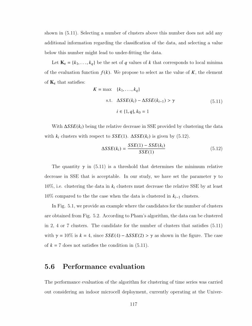
shown in (5.11). Selecting a number of clusters above this number does not add any

additional information regarding the classification of the data, and selecting a value

below this number might lead to under-fitting the data.

Let Kc = {k1, . . . , kq} be the set of q values of k that corresponds to local minima

of the evaluation function f (k). We propose to select as the value of K , the element

of Kc that satisfies:

K = max {k1, . . . , kq}

s.t. ∆SSE(ki) − ∆SSE(ki−1) > γ

i ∈ {1, q}, k0 = 1

(5.11)

With ∆SSE(ki) being the relative decrease in SSE provided by clustering the data

with ki clusters with respect to SSE(1). ∆SSE(ki) is given by (5.12).

∆SSE(ki) =SSE(1) − SSE(ki)

SSE(1)(5.12)

The quantity γ in (5.11) is a threshold that determines the minimum relative

decrease in SSE that is acceptable. In our study, we have set the parameter γ to

10%, i.e. clustering the data in ki clusters must decrease the relative SSE by at least

10% compared to the the case when the data is clustered in ki−1 clusters.

In Fig. 5.1, we provide an example where the candidates for the number of clusters

are obtained from Fig. 5.2. According to Pham’s algorithm, the data can be clustered

in 2, 4 or 7 clusters. The candidate for the number of clusters that satisfies (5.11)

with γ = 10% is k = 4, since SSE(4) − ∆SSE(2) > γ as shown in the figure. The case

of k = 7 does not satisfies the condition in (5.11).

5.6 Performance evaluation

The performance evaluation of the algorithm for clustering of time series was carried

out considering an indoor microcell deployment, currently operating at the Univer-

117

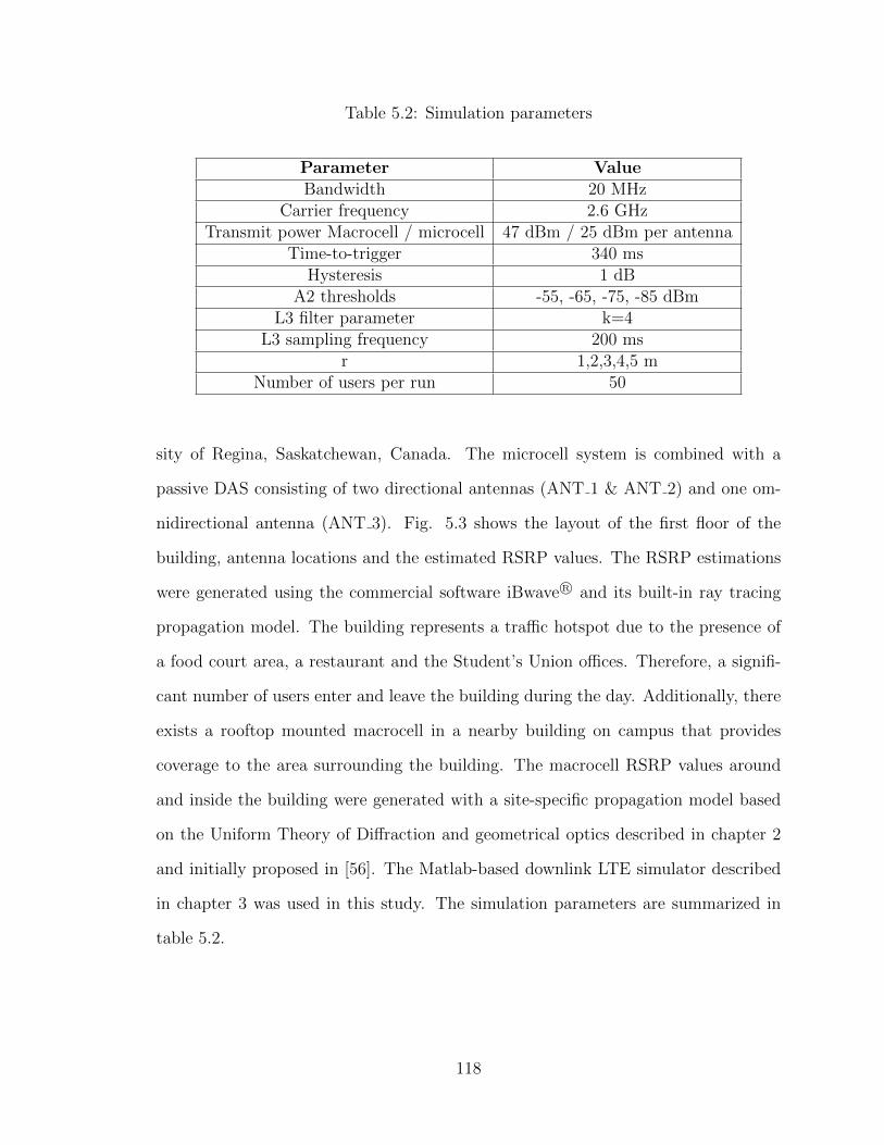
Table 5.2: Simulation parameters

Parameter ValueBandwidth 20 MHz

Carrier frequency 2.6 GHzTransmit power Macrocell / microcell 47 dBm / 25 dBm per antenna

Time-to-trigger 340 msHysteresis 1 dB

A2 thresholds -55, -65, -75, -85 dBmL3 filter parameter k=4

L3 sampling frequency 200 msr 1,2,3,4,5 m

Number of users per run 50

sity of Regina, Saskatchewan, Canada. The microcell system is combined with a

passive DAS consisting of two directional antennas (ANT 1 & ANT 2) and one om-

nidirectional antenna (ANT 3). Fig. 5.3 shows the layout of the first floor of the

building, antenna locations and the estimated RSRP values. The RSRP estimations

were generated using the commercial software iBwave R© and its built-in ray tracing

propagation model. The building represents a traffic hotspot due to the presence of

a food court area, a restaurant and the Student’s Union offices. Therefore, a signifi-

cant number of users enter and leave the building during the day. Additionally, there

exists a rooftop mounted macrocell in a nearby building on campus that provides

coverage to the area surrounding the building. The macrocell RSRP values around

and inside the building were generated with a site-specific propagation model based

on the Uniform Theory of Diffraction and geometrical optics described in chapter 2

and initially proposed in [56]. The Matlab-based downlink LTE simulator described

in chapter 3 was used in this study. The simulation parameters are summarized in

table 5.2.

118

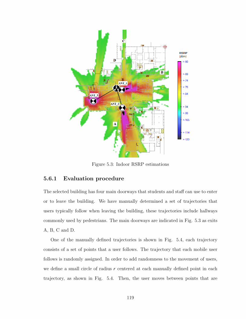
Figure 5.3: Indoor RSRP estimations

5.6.1 Evaluation procedure

The selected building has four main doorways that students and staff can use to enter

or to leave the building. We have manually determined a set of trajectories that

users typically follow when leaving the building, these trajectories include hallways

commonly used by pedestrians. The main doorways are indicated in Fig. 5.3 as exits

A, B, C and D.

One of the manually defined trajectories is shown in Fig. 5.4, each trajectory

consists of a set of points that a user follows. The trajectory that each mobile user

follows is randomly assigned. In order to add randomness to the movement of users,

we define a small circle of radius r centered at each manually defined point in each

trajectory, as shown in Fig. 5.4. Then, the user moves between points that are

119

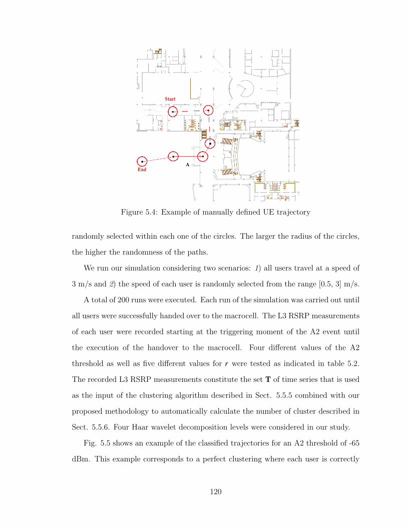
Figure 5.4: Example of manually defined UE trajectory

randomly selected within each one of the circles. The larger the radius of the circles,

the higher the randomness of the paths.

We run our simulation considering two scenarios: 1) all users travel at a speed of

3 m/s and 2) the speed of each user is randomly selected from the range [0.5, 3] m/s.

A total of 200 runs were executed. Each run of the simulation was carried out until

all users were successfully handed over to the macrocell. The L3 RSRP measurements

of each user were recorded starting at the triggering moment of the A2 event until

the execution of the handover to the macrocell. Four different values of the A2

threshold as well as five different values for r were tested as indicated in table 5.2.

The recorded L3 RSRP measurements constitute the set T of time series that is used

as the input of the clustering algorithm described in Sect. 5.5.5 combined with our

proposed methodology to automatically calculate the number of cluster described in

Sect. 5.5.6. Four Haar wavelet decomposition levels were considered in our study.

Fig. 5.5 shows an example of the classified trajectories for an A2 threshold of -65

dBm. This example corresponds to a perfect clustering where each user is correctly

120

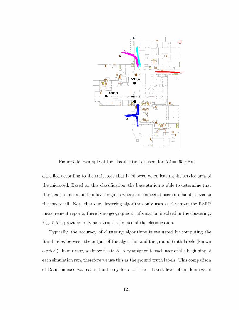
ANT_1

ANT_2ANT_3

Figure 5.5: Example of the classification of users for A2 = -65 dBm

classified according to the trajectory that it followed when leaving the service area of

the microcell. Based on this classification, the base station is able to determine that

there exists four main handover regions where its connected users are handed over to

the macrocell. Note that our clustering algorithm only uses as the input the RSRP

measurement reports, there is no geographical information involved in the clustering,

Fig. 5.5 is provided only as a visual reference of the classification.

Typically, the accuracy of clustering algorithms is evaluated by computing the

Rand index between the output of the algorithm and the ground truth labels (known

a priori). In our case, we know the trajectory assigned to each user at the beginning of

each simulation run, therefore we use this as the ground truth labels. This comparison

of Rand indexes was carried out only for r = 1, i.e. lowest level of randomness of

121

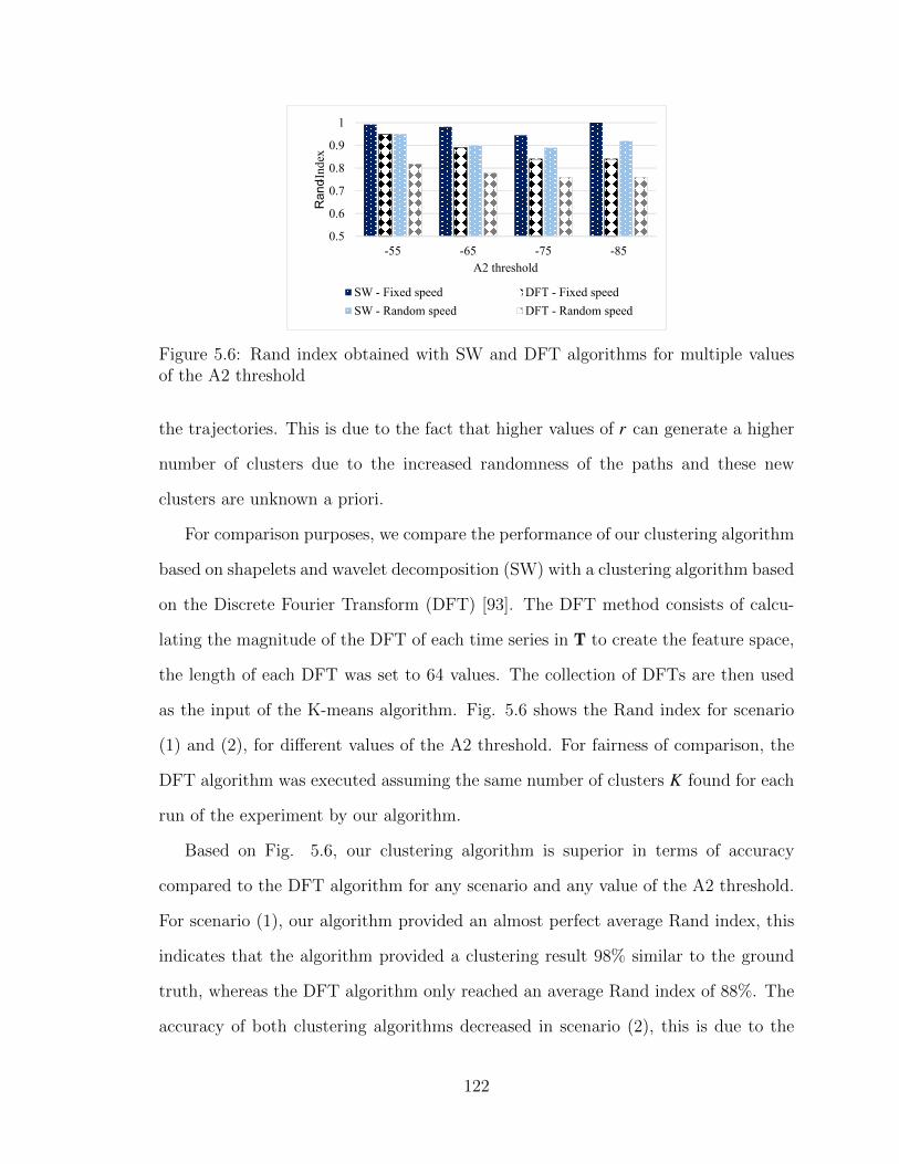
0.5

0.6

0.7

0.8

0.9

1

-55 -65 -75 -85

Rand-

Inde

x

A2 threshold

SW - Fixed speed DFT - Fixed speed

SW - Random speed DFT - Random speed

Figure 5.6: Rand index obtained with SW and DFT algorithms for multiple valuesof the A2 threshold

the trajectories. This is due to the fact that higher values of r can generate a higher

number of clusters due to the increased randomness of the paths and these new

clusters are unknown a priori.

For comparison purposes, we compare the performance of our clustering algorithm

based on shapelets and wavelet decomposition (SW) with a clustering algorithm based

on the Discrete Fourier Transform (DFT) [93]. The DFT method consists of calcu-

lating the magnitude of the DFT of each time series in T to create the feature space,

the length of each DFT was set to 64 values. The collection of DFTs are then used

as the input of the K-means algorithm. Fig. 5.6 shows the Rand index for scenario

(1) and (2), for different values of the A2 threshold. For fairness of comparison, the

DFT algorithm was executed assuming the same number of clusters K found for each

run of the experiment by our algorithm.

Based on Fig. 5.6, our clustering algorithm is superior in terms of accuracy

compared to the DFT algorithm for any scenario and any value of the A2 threshold.

For scenario (1), our algorithm provided an almost perfect average Rand index, this

indicates that the algorithm provided a clustering result 98% similar to the ground

truth, whereas the DFT algorithm only reached an average Rand index of 88%. The

accuracy of both clustering algorithms decreased in scenario (2), this is due to the

122

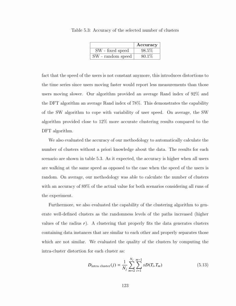
Table 5.3: Accuracy of the selected number of clusters

AccuracySW - fixed speed 98.5%

SW - random speed 80.1%

fact that the speed of the users is not constant anymore, this introduces distortions to

the time series since users moving faster would report less measurements than those

users moving slower. Our algorithm provided an average Rand index of 92% and

the DFT algorithm an average Rand index of 78%. This demonstrates the capability

of the SW algorithm to cope with variability of user speed. On average, the SW

algorithm provided close to 12% more accurate clustering results compared to the

DFT algorithm.

We also evaluated the accuracy of our methodology to automatically calculate the

number of clusters without a priori knowledge about the data. The results for each

scenario are shown in table 5.3. As it expected, the accuracy is higher when all users

are walking at the same speed as opposed to the case when the speed of the users is

random. On average, our methodology was able to calculate the number of clusters

with an accuracy of 89% of the actual value for both scenarios considering all runs of

the experiment.

Furthermore, we also evaluated the capability of the clustering algorithm to gen-

erate well-defined clusters as the randomness levels of the paths increased (higher

values of the radius r). A clustering that properly fits the data generates clusters

containing data instances that are similar to each other and properly separates those

which are not similar. We evaluated the quality of the clusters by computing the

intra-cluster distortion for each cluster as:

Dintra cluster( j) =1

N j

Nj∑m=2

m−1∑i=1

sD(Ti,Tm) (5.13)

123

Where N j is the number of time series in cluster j. Note that the time series in

the cluster should be sorted in ascending order of length before applying (5.13). The

quantity Dintra cluster( j) represents the average subsequence distance between time

series that belong to the same cluster. We calculate the total average intra-cluster

distortion DT as:

DT =1

K

K∑j=1

Dintra cluster( j) (5.14)

Where K is the number of clusters. Ideally, low values of DT are preferred since

they indicate well-defined clusters.

Fig. 5.7 and 5.8 show the average DT for each scenario as a function of the

values of r. For scenario (1), the values of DT generated by the SW algorithm are

significantly below the ones provided by the DFT algorithm, this indicates that each

cluster provided by the SW algorithm contains highly similar time series. A similar

result is observed in scenario (2), where both algorithms provided lower DT due to

the fact that the speed of users is random and this introduces variability in the time

series, therefore the number of clusters is higher and this leads to lower values of DT

as compared to scenario (1). However, the SW algorithm still provides better defined

clusters for this scenario. The total average of DT per scenario are shown in Fig. 5.9,

our clustering algorithm was able to provide clusters with an improvement of 75% in

the total average intra-cluster distortion for both scenarios.

5.7 Summary

In this chapter we have proposed a methodology that allows base stations to auto-

matically and autonomously discover the RF conditions of its cell-edge. We propose

the use of machine learning and data mining techniques to identify patterns in the

RSRP measurement reports submitted by users as they approach the cell-edge. Our

124

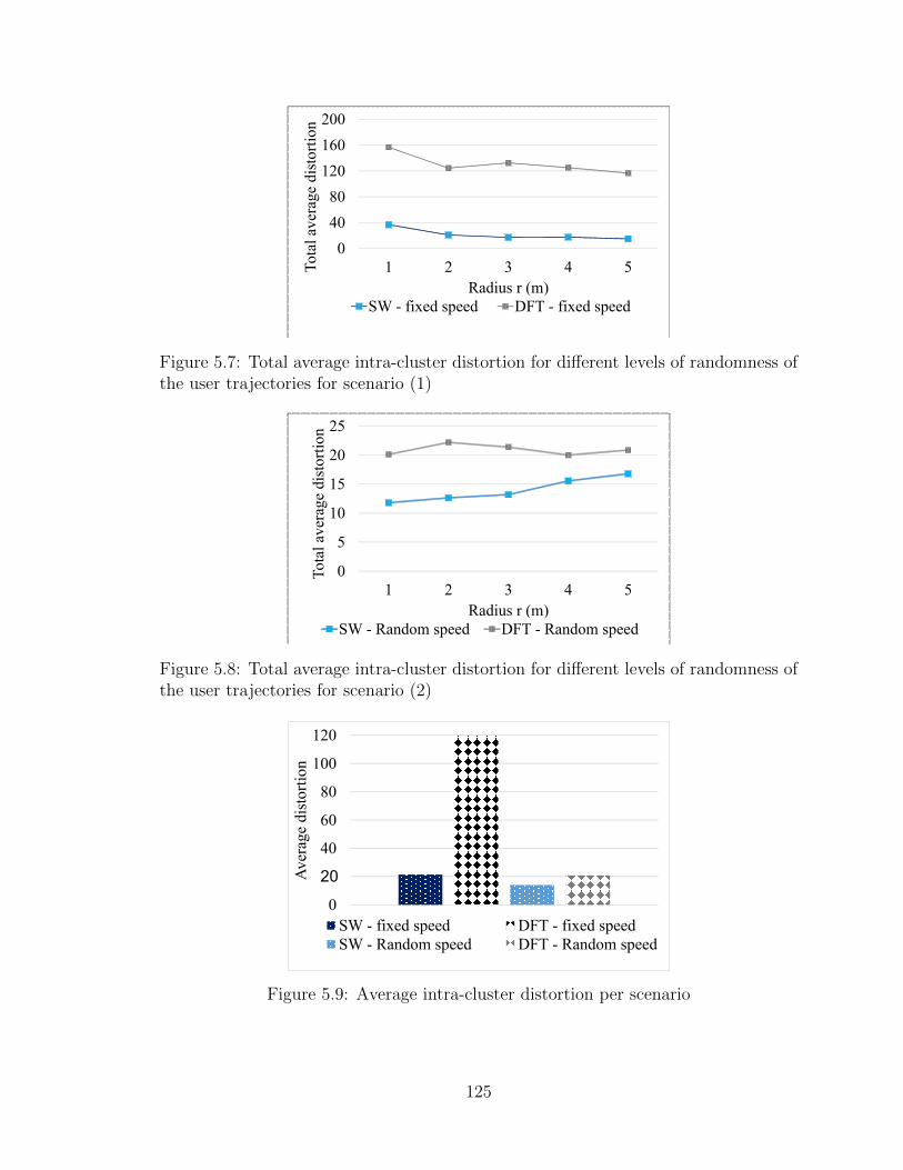
0

40

80

120

160

200

1 2 3 4 5Tota

l ave

rage

dis

tort

ion

Radius r (m)SW - fixed speed DFT - fixed speed

Figure 5.7: Total average intra-cluster distortion for different levels of randomness ofthe user trajectories for scenario (1)

0

5

10

15

20

25

1 2 3 4 5

Tota

l ave

rage

dis

tort

ion

Radius r (m)SW - Random speed DFT - Random speed

Figure 5.8: Total average intra-cluster distortion for different levels of randomness ofthe user trajectories for scenario (2)

0

20

40

60

80

100

120

Ave

rage

dis

tort

ion

SW - fixed speed DFT - fixed speedSW - Random speed DFT - Random speed

Figure 5.9: Average intra-cluster distortion per scenario

125

simulations considered an LTE network consisting of a macrocell and a indoor micro-

cell. Our clustering algorithm based on unsupervised-shapelets and multi-resolution

wavelet decomposition (SW) provided superior performance compared to a DFT-

based clustering algorithm. Our algorithm SW was able to provide clustering results

close to 12% more accurate and up to 75% better quality of clusters. Furthermore,

our methodology to automatically determine the number of clusters without any prior

knowledge was able to achieve an accuracy close to 90%.

126

Chapter 6

Optimization of handoverparameters for in-building systems

The optimization of handover parameters for in-building systems is investigated in

this chapter. We propose a novel methodology that provides in-building base stations

with the flexibility to customize handover parameters to specific radio frequency con-

ditions at the cell-edge for different loading scenarios. We propose the use of machine

learning and data mining techniques to allow the base stations to autonomously learn

and identify characteristic patterns in the received signal strength values (reported

by users during the handover process), and apply optimal HO parameters for each

case. Our optimization strategy jointly considers the radio frequency conditions at

the cell-edge and the load levels of the base stations, to determine optimal handover

parameters that maximize the quality of service and guarantee the continuity of ser-

vice at the cell-edge. We evaluated our methodology with experimental data collected

from two fully operational LTE in-building systems deployed in a university campus.

Our results show that with our methodology the spectral efficiency at the cell-edge

can be greatly improved. Downlink data rate gains at the cell-edge reached a value

close to 150% for a certain loading scenario compared to the traditional approach of

selecting a unique set of handover parameters for the entire in-building system.

6.1 Introduction

Nowadays, in-building systems are being largely deployed in different venues like:

shopping centers, airports, stadiums and university campuses. However, the opti-

127

mization of handover parameters in in-building systems is a challenging task for net-

work operators, especially due to the nature of HetNets that combine low power and

high power base stations. Typically, operators define the handover parameters with

the objective of guarantying the continuity of service at the cell edge. However, with

the implementation of new technologies like VoLTE, the quality of service provided

to users as they move between coverage areas becomes also a relevant aspect.

In this chapter, we propose a methodology to optimize the handover parameters

of in-building systems. In order to determine the optimal values of the handover

parameters, such methodology jointly considers two essential factors in HetNets: RF

conditions at the cell-edge and load level of the cells. Our approach comes to answer

the question of how late or how early a handover can be executed in order to maxi-

mize the quality of service at the cell-edge while reducing handover failures and the

triggering of unnecessary handovers.

We propose the use of machine learning and data mining techniques to allow

the in-building system to autonomously learn and identify characteristic patterns in

the signal strength received from users as they approach the cell-edge (as described

in chapter 5), and apply optimal HO parameters for each case. We evaluated the

performance of our approach with experimental data collected from fully operational

LTE in-building systems.

The rest of the chapter is organized as follows: in Sect. 6.2 we describe the main

handover optimization strategies currently proposed in the literature. In Sect. 6.3

we describe the contributions of the work presented in this chapter. In Sect. 6.4 we

describe the handover procedure in LTE systems. We provide a detailed description of

our methodology to optimize handover parameters in Sect. 6.5. In Sect. 6.6 and 6.7

we provide details regarding our experimental setup and the performance evaluation

of our methodology, respectively. Finally, we provide a summary in Sect. 6.8.

128

6.2 Related work

The development of self-optimizing strategies in cellular networks have attracted sig-

nificant interest in the research community in recent years, in particular strategies

related to the self-optimization of mobility parameters (e.g. Mobility Robustness Op-

timization - MRO). Such strategies are intended to automate the adjustment of HO

parameters. In [47], one of the most influential approaches for the automatic opti-

mization of handover parameters is described. The approach consists of the selection

of suitable handover parameters based on the continuous monitoring of specific per-

formance indicators (e.g. handover failure ratio and the ping-pong ratio). If any of the

performance indicators exceeds a certain predefined threshold, the base station incre-

mentally modifies the handover parameters until the performance indicator reaches

an acceptable level. This approach has a slow response to changes since it requires

the collection of a large number of handover statistics to trigger the modification of

the handover parameters [48]. For example, a number of handover failures must occur

before the algorithm adjusts the parameters. In [49, 50] the authors have proposed

similar handover optimization strategies. These approaches propose the application

of a single set of parameters for each cell.

In [48, 51], the authors modified the approach in [47], by defining new metrics in

addition to the performance indicators in [47]. The authors called such indicators

“soft-metrics” (e.g. handover command transmission time). Their objective was

to improve the capability of the algorithm to quickly react to handover failures by

defining metrics which are strongly correlated with the increase in handover failures.

Hence, the optimization algorithm is triggered by observing the soft-metrics instead

of the performance indicators as it is done in [47].

In [52], the authors propose an analytical method to determine handover param-

eters, specifically the RSRP threshold used to trigger handovers and a timer used to

129

avoid the triggering of unnecessary handovers (time-to-trigger). They define a math-

ematical expression that relates the time-to-trigger (TTT) with the variance of the

RSRP measurements reported by the mobiles. A large value of the variance of the

RSRP values indicates a higher chance of triggering unnecessary handovers, hence

larger TTT values are required. To determine the RSRP threshold, they apply the

Page Hinkley test to detect the RSRP level at which the neighboring cell becomes

stronger than the serving cell, at such level the handover should be triggered to avoid

handover failures. The handover parameters are adapted to changes in performance

indicators with an iterative algorithm based on simulated annealing. This is one of

the first approaches that propose analytical expressions for the handover parameters

in homogeneous networks.

The idea of adapting the handover parameters to specific cell-edge conditions in

HetNets was initially investigated in [46]. The authors proposed a methodology to

deal with the specific challenges found in HetNets (e.g. uneven interference levels at

the cell edge). They propose to allow the base station to determine the best moment

to initiate the request of the handover to the target cell. In their approach, the

base station monitors the values of CQI reported by users as they approach the cell-

edge and the handover is initiated when the reported CQI falls under a predefined

threshold. The CQI values are directly related to the SINR. With this approach,

the handovers are not triggered based on a unique value of a received signal strength

threshold, instead the actual RF conditions of the cell edge determine the moment

when the handover is initiated.

In [53], the authors propose to use different sets of handover parameters based

on the type of base station in a HetNet. According to their study, in macrocell-only

networks, the overlap between coverage areas is larger, hence conservative handover

parameters can be applied. However, the overlap between macrocells and smalls cells

(e.g. macro-to-pico) or even among small cells (pico-to-pico) tend to be smaller,

130

therefore more aggressive handover parameters are required to avoid link failures.

In [54], the authors propose to customize handover parameters based on user behavior.

They proposed to categorize users according to their speed and their type of traffic

(real time or non-real time). The handover parameters are then optimized for each

category following an approach similar to [47].

Our approach has been inspired by the fact that a single set of handover parame-

ters provides suboptimal values of the handover performance indicators, particularly

in HetNets, as stated in [46]. We consider that the handover parameters should be

optimized according to the actual RF conditions at the cell-edge. But also, the opti-

mization should jointly consider the loading conditions of the cells. This is required

in order to provide the highest quality of service possible as users approach the edge

of the cell. This is a factor that is typically ignored by the methodologies proposed in

the literature. Our approach comes to answer the question of how late or how early a

handover can be executed in order to maximize the quality of service at the cell-edge

while reducing handover failures and the triggering of unnecessary handovers.

The key factor of our approach is the application of machine learning and data

mining techniques to classify users in clusters based on their mobility behavior and

the application of optimal handover parameters for each cluster. A similar idea was

introduced by Sas et al. in [55]. In their work, the authors proposed the collection of

RSRP measurement reports submitted by a limited set of users, labeled as “reference

users”, as they move along the service area of a homogeneous network with multiple

macrocells. Their objective was to match the RSRP measurement reports from new

users to those reports previously collected from the reference users. If a user is

matched to one of the reference reports, then it is assumed that this user will follow

the same trajectory as the matched reference user.

Our approach substantially advances the idea in [55], specifically in the context

of in-building systems. We propose the application of the clustering algorithm pro-

131

posed in chapter 5 to identify patterns in the RSRP measurements reports submitted

by multiple users as they leave the service area. We use such patterns to cluster the

measurement reports and identify the RF propagation conditions that users, following

such archetypal trajectories, are subject to. Then, we find optimal handover param-

eters for each cluster by jointly taking into consideration the specific RF conditions

of each cluster and the loading conditions of the serving and target cell. The authors

in [55] only treated the problem of matching measurement reports to a reference and

did not provide a methodology for the optimization of handover parameters.

6.3 Contributions

The contributions of this chapter can be summarized in two main points:

1. We propose a novel methodology to optimize handover parameters for in-

building systems. The key insight behind such methodology is the adjustment

of handover parameters based on the knowledge that base stations are able to

acquire regarding the RF conditions of their cell-edge. This knowledge is ob-

tained through the application of the clustering algorithm proposed in chapter

5. The objective of our methodology is to maximize the quality of service while

guarantying the continuity of service at the cell-edge.

2. Our methodology can also be considered as a load balancing approach for users

in connected mode. This is due to the fact that the optimization strategy not

only takes into consideration the levels of interference at the cell-edge but also

the loading conditions of the serving and target cell. The handover parameters

are then adjusted accordingly in order to provide the highest quality of service

possible.

132

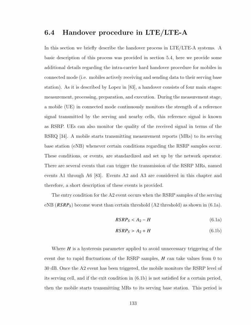
6.4 Handover procedure in LTE/LTE-A

In this section we briefly describe the handover process in LTE/LTE-A systems. A

basic description of this process was provided in section 5.4, here we provide some

additional details regarding the intra-carrier hard handover procedure for mobiles in

connected mode (i.e. mobiles actively receiving and sending data to their serving base

station). As it is described by Lopez in [83], a handover consists of four main stages:

measurement, processing, preparation, and execution. During the measurement stage,

a mobile (UE) in connected mode continuously monitors the strength of a reference

signal transmitted by the serving and nearby cells, this reference signal is known

as RSRP. UEs can also monitor the quality of the received signal in terms of the

RSRQ [34]. A mobile starts transmitting measurement reports (MRs) to its serving

base station (eNB) whenever certain conditions regarding the RSRP samples occur.

These conditions, or events, are standardized and set up by the network operator.

There are several events that can trigger the transmission of the RSRP MRs, named

events A1 through A6 [83]. Events A2 and A3 are considered in this chapter and

therefore, a short description of these events is provided.

The entry condition for the A2 event occurs when the RSRP samples of the serving

eNB (RSRPS) become worst than certain threshold (A2 threshold) as shown in (6.1a).

RSRPS < A2 − H (6.1a)

RSRPS > A2 + H (6.1b)

Where H is a hysteresis parameter applied to avoid unnecessary triggering of the

event due to rapid fluctuations of the RSRP samples, H can take values from 0 to

30 dB. Once the A2 event has been triggered, the mobile monitors the RSRP level of

its serving cell, and if the exit condition in (6.1b) is not satisfied for a certain period,

then the mobile starts transmitting MRs to its serving base station. This period is

133

the parameter called time-to-trigger. The frequency of transmission of the MRs is

defined by the network operator, in actual systems it is typically set to one MR every

200ms or 300ms.

On the other hand, the entry condition of the event A3 occurs when the RSRP

level of a neighboring cell (RSRPN) is above RSRPS plus a threshold (A3 threshold)

as shown in (6.2a).

RSRPN > RSRPS + A3 + H (6.2a)

RSRPN > RSRPS + A3 − H (6.2b)

Once again, after the A3 event has been triggered, if the exit condition in (6.2b)

is not satisfied during the TTT period, then the UE starts the transmission of MRs

to its serving cell.

During the processing stage of the handover, the serving base station evaluates the

MRs transmitted by the mobile and defines the target cell (usually the neighboring

cell with the strongest RSRP level in the MRs). It will then contact the target cell

to request a handover. The target cell executes admission control procedures and

accepts or rejects the request. If the request is accepted, then the target cell starts

the preparation stage of the handover and sends an “HO request acknowledgment”

to the serving cell. When this acknowledgment is received, the serving cell sends an

“HO command” to the mobile. At this point, the serving base station releases any

radio resources assigned to the mobile and the connection with the mobile is ended.

Finally, during the execution stage of the handover, the mobile tries to establish

a connection with the target cell using a random access procedure. If the connection

is successful, then the handover is completed and the target cell starts transmitting

data to the mobile.

The A2 or A3 thresholds, hysteresis H and TTT timer are fundamental parameters

that control the HO process. These parameters need to be optimized by network

134

operators for specific network conditions in order to guarantee the continuity of service

as users move between coverage areas (i.e. to reduce HO failures).

Handover failures can occur when the handover is executed too late, too early or

when it is executed to the wrong target cell. A too late handover occurs when the

signal from the serving cell degrades below a minimum acceptable level before the

mobile is able to receive the “HO command”. On the other hand, a too early handover

occurs when the communication with the target cell is not strong enough yet when

the mobile tries to establish a connection using the random access procedure. And

finally, in some cases the target cell is wrongly selected by the serving base station,

usually this is due to an error in the list of neighboring cells. In this case the mobile

will not be able to complete the handover since the target cell is likely out of its

uplink range. When handover failures happen, there is an abrupt discontinuity of the

service and a connection re-establishment procedure has to be executed by the mobile,

as a result, the quality of service is negatively affected and this leads to subscriber

dissatisfaction.

The occurrence of handover failures can be reduced or even eliminated with the

application of optimal HO parameters. A reduction of the TTT helps reduce too

late HOs since the handover is executed faster. However, a small TTT increases the

chances of ping-pong events (i.e. UE is handed over back and forth from the serving

eNB and the target eNB over a short period), this is undesirable since it increases the

signaling load in the network due to unnecessary HO operations. Therefore, these

types of trade-offs have to be considered during the optimization process. Further-

more, the current HO procedure described in this section does not take into consid-

eration the quality of service provided to the mobile users as they cross the edge of

the service area. Such quality of service is not only affected by the HO parameters

but also by the dynamic loading conditions of both the serving and target cell.

In the next sections, we describe our proposed methodology to optimize the han-

135

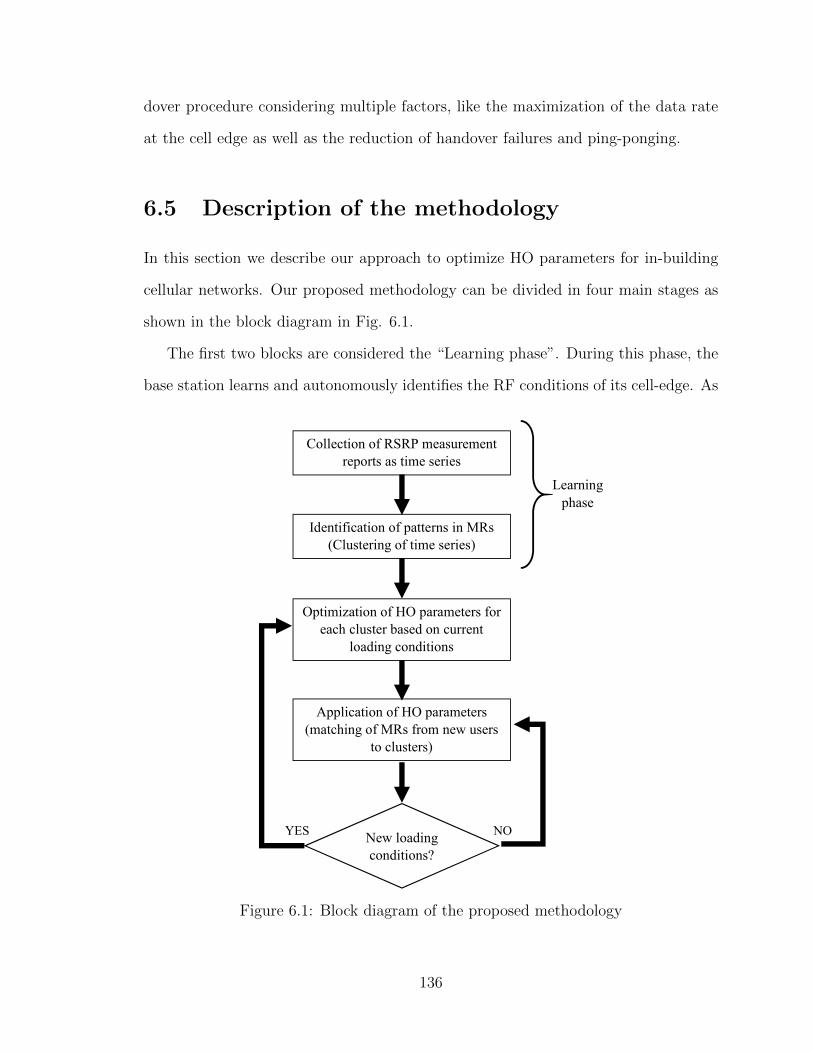
dover procedure considering multiple factors, like the maximization of the data rate

at the cell edge as well as the reduction of handover failures and ping-ponging.

6.5 Description of the methodology

In this section we describe our approach to optimize HO parameters for in-building

cellular networks. Our proposed methodology can be divided in four main stages as

shown in the block diagram in Fig. 6.1.

The first two blocks are considered the “Learning phase”. During this phase, the

base station learns and autonomously identifies the RF conditions of its cell-edge. As

Collection of RSRP measurement

reports as time series

Identification of patterns in MRs

(Clustering of time series)

Optimization of HO parameters for

each cluster based on current

loading conditions

Application of HO parameters

(matching of MRs from new users

to clusters)

New loading

conditions?

YES NO

Learning

phase

Figure 6.1: Block diagram of the proposed methodology

136

it was mentioned before, the cell-edge of in-building systems is highly irregular and

subject to uneven levels of interference caused by the outdoor macrocells.

The first stage of the methodology consists of the collection of measurements

reports transmitted by users that were successfully handed over to another cell. We

consider the RSRP values, from the MRs sent by the UEs, as a collection of time series

that can be used to identify archetypal movements of users in indoor environments,

particularly as users exit the building. As pointed out in [55], users that move along

similar trajectories will transmit measurement reports that are highly correlated with

each other. In the case of indoor environments, the movement of users as they leave

the building is somewhat predefined, as people tend to exit the building walking

through doors whose locations remain unchanged. Hence, mobiles following a similar

paths will likely experience similar RF conditions during the handover to the outdoor

macrocell. Therefore, we propose to automatically identify patterns in the MRs that

will allow the base station to determine the typical RF conditions of the environment

as users approach its cell-edge. In order to identify such patterns, we propose the use

of machine learning and data mining techniques. For this purpose, in our methodology

we apply the clustering algorithm proposed in chapter 5. This automatic identification

of patterns in the MRs corresponds to the second block of the learning phase.

Once the base station has clustered the set of MRs according to the identified

characteristic patterns, we propose to calculate optimal values of the HO parameters

for each one of the clusters found. Typically, each cluster of MRs corresponds to a

section of the cell-edge with very distinctive characteristics. For example, consider

these two cases: 1) one of the clusters of MRs corresponds to a group of users where the

RSRP from the serving eNB decreased sharply as they walk out of the building and the

signal from the outdoor macrocell increased rapidly, 2) another cluster corresponds to

a set of users where the degradation of the signal from the serving cell was rather slow

and the signal from the macrocell also increased slowly as users left the building. For

137

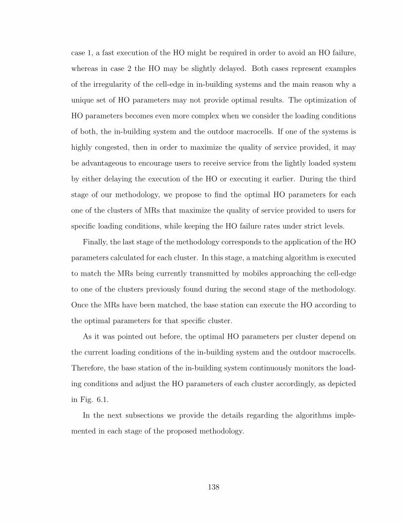
case 1, a fast execution of the HO might be required in order to avoid an HO failure,

whereas in case 2 the HO may be slightly delayed. Both cases represent examples

of the irregularity of the cell-edge in in-building systems and the main reason why a

unique set of HO parameters may not provide optimal results. The optimization of

HO parameters becomes even more complex when we consider the loading conditions

of both, the in-building system and the outdoor macrocells. If one of the systems is

highly congested, then in order to maximize the quality of service provided, it may

be advantageous to encourage users to receive service from the lightly loaded system

by either delaying the execution of the HO or executing it earlier. During the third

stage of our methodology, we propose to find the optimal HO parameters for each

one of the clusters of MRs that maximize the quality of service provided to users for

specific loading conditions, while keeping the HO failure rates under strict levels.

Finally, the last stage of the methodology corresponds to the application of the HO

parameters calculated for each cluster. In this stage, a matching algorithm is executed

to match the MRs being currently transmitted by mobiles approaching the cell-edge

to one of the clusters previously found during the second stage of the methodology.

Once the MRs have been matched, the base station can execute the HO according to

the optimal parameters for that specific cluster.

As it was pointed out before, the optimal HO parameters per cluster depend on

the current loading conditions of the in-building system and the outdoor macrocells.

Therefore, the base station of the in-building system continuously monitors the load-

ing conditions and adjust the HO parameters of each cluster accordingly, as depicted

in Fig. 6.1.

In the next subsections we provide the details regarding the algorithms imple-

mented in each stage of the proposed methodology.

138

6.5.1 Collection of measurement reports

During this initial stage, the base station collects measurement reports transmitted by

users that were successfully handed over to another cell. These measurement reports

are considered as time series and will be used as input to the clustering algorithm

described in the next subsection.

As users walk outside the coverage area of the in-building system, two main situa-

tions happen as part of the handover process: 1) the triggering of the transmission of

MRs and 2) the actual moment when the base station transmits the HO request mes-

sage to the target cell. These situations mark the beginning and the end moment of

the collection of RSRP samples from the measurement reports transmitted by users.

In order to facilitate the collection of enough MRs per mobile (for clustering

purposes), we propose the use of event A2 to trigger the transmission of measuring

reports (see Sect. 6.4). Furthermore, we propose the use of the A3 event to determine

the actual moment when the base station requests the HO to the target cell. This

means that the base station monitors the RSRP samples in the MRs and looks for

the occurrence of an A3 event. Once the entry condition in (6.2a) holds for a TTT

period, then the HO is actually requested to the target cell and the base station stops

the collection of MRs from the user. Hence, the triggering of an A3 event determines

the end of the collection of MRs from the mobile.

The MRs collected from a user constitute a time series. The base station should

be able to collect enough time series such that the relevant characteristic patterns

(clusters) can be found by the clustering algorithm. In most cases, due to the fact

that in-building systems are deployed to provide service to high traffic areas, this

collection of time series can occur relatively fast during the first hours of operation

of the system.

139

6.5.2 Clustering of time series

In order to automatically identify patterns in the MRs, a clustering algorithm is

applied by the base station of the in-building system. In this study we propose to

apply the clustering algorithm that we developed in our previous work in [60]. The

details of this algorithm can be found in chapter 5.

6.5.3 Optimization of handover parameters

With the identification of clusters in the collected MRs, the base station of the in-

building system is able to learn the radio frequency conditions of the paths that users

follow when they leave the building, without actually knowing their physical location.

Each one of the identified clusters has very specific characteristics in terms of the

behavior of the RSRP. In some cases, the RSRP at the cell-edge decreases sharply

while in other cases a slow decrease occurs. The insight of our approach to optimize

HO parameters, is to find suitable values for the TTT and A3 threshold to guarantee

the continuity of service at the cell edge (i.e. avoid HO failures) for users whose

MRs follow a similar pattern as one of the identified cluster of RSRP measurements.

This means that the base station customizes the HO parameters according to the

specific RF conditions of the cell edge that such users will be subject to as they leave

the building. Furthermore, in our approach we do not only find values of the HO

parameters that will reduce or eliminate HO failures and ping-ponging but also the

quality of service provided at the cell edge is taken into consideration. Therefore,

our methodology is a much more comprehensive approach than the ones currently

proposed in the literature as described in Sect. 6.2, where the typical objective is to

find a unique set of HO parameters that reduces HO failures. With our methodology,

base stations are able to determine how late or how early an HO can be executed

with minimum degradation of the quality of service while guaranteeing the continuity

140

of service at the cell edge.

In order to reduce HO failures and ping-ponging for the specific cell-edge condi-

tions of each cluster of MRs, the behavior of the RSRP from the serving cell as well

as the target cell has to be evaluated. This is due to the fact that the RF conditions

of the cell-edge are one of the main factors that affect the success of the handovers.

However, in order to maximize the quality of service provided to users as they walk

through the cell-edge, the loading conditions of the serving and target cell becomes

a vital factor. Our approach combines the evaluation of these two factors: RF condi-

tions at the cell-edge and loading conditions of the cells. For example, a large value

of the A3 threshold or long TTT allows the base station to delay the execution of

the handover, this might be necessary in order to provide an acceptable data rate

if the target cell is congested. On the other hand, a small value of the A3 thresh-

old or short TTT allows the base station to execute the HO earlier, which might be

necessary when the serving cell is the one congested. However, how early or how

late the HO can be executed is limited by the cell-edge conditions, therefore both

factors are coupled and this fact has to be considered when the optimization of the

HO parameters is carried out. Our approach provides an answer to this problem, by

determining suitable values for the A3 threshold and the TTT such that data rates

are maximized and the HO failure rate is kept under a desired level.

In the next subsection we proceed to describe the formulation of the optimization

problem.

6.5.3.1 Formulation of the optimization problem

Our optimization strategy consists of the definition of an objective function Gk asso-

ciated with the kth cluster of MRs. This function has four terms, each one of them

corresponds to one performance indicator (PI). The first PI corresponds to the quality

of service that mobiles receive as they go through the edge of the cell. The second PI

141

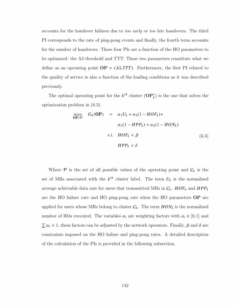
accounts for the handover failures due to too early or too late handovers. The third

PI corresponds to the rate of ping-pong events and finally, the fourth term accounts

for the number of handovers. These four PIs are a function of the HO parameters to

be optimized: the A3 threshold and TTT. These two parameters constitute what we

define as an operating point OP = (A3,TTT ). Furthermore, the first PI related to

the quality of service is also a function of the loading conditions as it was described

previously.

The optimal operating point for the kth cluster (OP∗k) is the one that solves the

optimization problem in (6.3).

maxOP∈P

Gk (OP) = α1Uk + α2(1 − HOFk )+

α3(1 − HPPk ) + α4(1 − HONk )

s.t. HOFk < β

HPPk < δ

(6.3)

Where P is the set of all possible values of the operating point and Ck is the

set of MRs associated with the kth cluster label. The term Uk is the normalized

average achievable data rate for users that transmitted MRs in Ck . HOFk and HPPk

are the HO failure rate and HO ping-pong rate when the HO parameters OP are

applied for users whose MRs belong to cluster Ck . The term HONk is the normalized

number of HOs executed. The variables αi are weighting factors with αi ∈ [0, 1] and∑αi = 1, these factors can be adjusted by the network operators. Finally, β and δ are

constraints imposed on the HO failure and ping-pong rates. A detailed description

of the calculation of the PIs is provided in the following subsection.

142

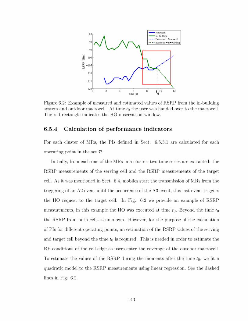
0 2 4 6 8 10 12120

115

110

105

100

95

90

85

time (s)

RS

RP

(dB

m)

Macrocell

In building

Estimated Macrocell

Estimated In building

t0

Figure 6.2: Example of measured and estimated values of RSRP from the in-buildingsystem and outdoor macrocell. At time t0 the user was handed over to the macrocell.The red rectangle indicates the HO observation window.

6.5.4 Calculation of performance indicators

For each cluster of MRs, the PIs defined in Sect. 6.5.3.1 are calculated for each

operating point in the set P.

Initially, from each one of the MRs in a cluster, two time series are extracted: the

RSRP measurements of the serving cell and the RSRP measurements of the target

cell. As it was mentioned in Sect. 6.4, mobiles start the transmission of MRs from the

triggering of an A2 event until the occurrence of the A3 event, this last event triggers

the HO request to the target cell. In Fig. 6.2 we provide an example of RSRP

measurements, in this example the HO was executed at time t0. Beyond the time t0

the RSRP from both cells is unknown. However, for the purpose of the calculation

of PIs for different operating points, an estimation of the RSRP values of the serving

and target cell beyond the time t0 is required. This is needed in order to estimate the

RF conditions of the cell-edge as users enter the coverage of the outdoor macrocell.

To estimate the values of the RSRP during the moments after the time t0, we fit a

quadratic model to the RSRP measurements using linear regression. See the dashed

lines in Fig. 6.2.

143

Additionally, not all the RSRP values are used for the calculation of PIs, we

only consider the RSRP values at the cell-edge. For this purpose, we define an “HO

observation window” with a duration of HOw seconds. This window is centered at

time t0 as shown in Fig. 6.2. Therefore, only RSRP values inside the window are

considered for the calculation of PIs. This guarantees that PIs, like the normalized

average achievable data rate, are only affected by the actual cell-edge conditions.

For each OP ∈ P, our algorithm calculates the number of HO failures, ping-pongs

and the number of handovers triggered for each set of MRs in a cluster. Given an

operating point, the algorithm looks for the triggering of A3 events considering the

RSRP values inside the “HO observation window” and determines if a handover can be

executed successfully. If the HO is not successful (either too late or too early HO), then

an HO failure is counted and the algorithm estimates if a connection re-establishment

can be executed to resume the service based on the RSRP values. Additionally, for

successful HOs the algorithm checks if a ping-pong event has occurred. Therefore, to

calculate these PIs the algorithm essentially simulates the four stages of the handover

process as described in Sect. 6.4, for the period of time corresponding to the “HO

observation window”.

The handover failure rate and ping-pong event rate for the kth cluster are calcu-

lated according to (6.4) and (6.5) respectively.

HOFk (OP) =Failk (OP)

Failk (OP) + Succk (OP)(6.4)

HPPk (OP) =PPk (OP)

Failk (OP) + Succk (OP)(6.5)

Where Failk (OP) and Succk (OP) are the total number of HO failures and the

total number of successful HOs for cluster k with operating point OP, and PPk (OP)

is the total number of ping-pong events.

The normalized number of HOs, HONk , is simply calculated as:

144

HONk (OP) =Failk (OP) + Succk (OP)

HONmaxk

(6.6)

Where HONmaxk is the maximum number of HOs for cluster k obtained with any

of the values of OP, i.e. HONmaxk = max ({HONk (OP) |OP ∈ P}).

Finally, we proceed to describe the calculation of the normalized average achiev-

able data rate Uk . The achievable data rate for a user depends on the SINR, and it

is typically calculated with the well-known Shannon Hartley theorem [27]:

R j = BW j log2(1 + SI N RS) [bps] (6.7)

Where the term BW j is the portion of the bandwidth (in Hz) allocated to the

user for downlink transmissions and j is the user identifier. SINRS is the ratio of

the received power from the serving cell and the total power of the interference re-

ceived from neighboring cells plus noise. In actual systems, the amount of bandwidth

allocated to a mobile depends on the total number of users currently connected to

the cell. In our algorithm, we assume that bandwidth resources are shared among

connected users based on a proportional fair scheduler. Additionally, as it was shown

in [27], in the long term, the resource allocation that maximizes the sum of the rates

for all users connected to a cell is “equal allocation”, i.e.:

BW j =BWS

NS(6.8)

Where BWS is the total bandwidth available at the serving cell and NS is the total

number of users actively connected to the cell.

The calculation of the average achievable data rate Rk j (OP) is carried out by

determining the actual serving cell for each time instant corresponding to an RSRP

value in the “HO observation window” when the HO parameters in OP are applied.

Multiple HOs could be detected during the observation window, therefore the serving

cell is subject to change according to the HO stages described in Sect. 6.4. Hence,

145

for each time instant corresponding to an RSRP value in the observation window,

the algorithm determines the current serving cell and SINR, and calculates the value

of R j according to (6.7) and (6.8). Finally, all the values of R j calculated during the

observation window are averaged to obtain Rk j (OP). It is important to mention, that

during the execution stage of the handover, the mobile tries to establish a connection

with the target cell using a random access procedure. During this stage of the HO,

the mobile is not actively receiving data, therefore its value of R j is set to zero until

the mobile is able to successfully complete the HO.

In order to calculate Rk j (OP) for each j ∈ Ck , the base station must know the

loading condition of the target cell, i.e. cells should exchange their current number

of connected users.

Finally, the normalized achievable data rate Uk used in the optimization problem

(6.3) is calculated as:

Uk =

∑j∈Ck Rk j (OP)/|Ck |

Umaxk

(6.9)

Where Umaxk = max ({Uk (OP) |OP ∈ P}).

Note that all the PIs can only take values in the interval [0, 1].

6.5.5 Solving the optimization problem

In our methodology, the set P corresponds to the set of possible values of the operating

point OP = (A3,TTT ). According to the 3GPP standard [34], the TTT can only take

a finite number of possible values up to 5120 ms. However, some of the large values

that TTT can take are typically not suitable for pedestrian environments, hence we

have reduced the possible values of TTT to:

TTT ∈ {80, 100, 128, 160, 256, 320, 480, 512, 640, 1024} (6.10)

146

Regarding the A3 threshold, in our methodology it can take the following values:

A3 ∈ {−4,−3,−2,−1, 0, 1, 2, 3, 4, 5, 6, 7} (6.11)

Positive values of the A3 threshold are useful to delay the execution of the han-

dover. On the other hand, allowing the A3 threshold to take negative values enables

the base station to execute the HO earlier.

Based on (6.10) and (6.11), the set P has a finite and tractable number of possible

values. In our approach we evaluate the objective function Gk for each PO ∈ P and

select the operating point that satisfies the problem in (6.3) for each cluster.

6.5.6 Matching of time series

In order to apply the optimal HO parameters found in the previous stage of our

methodology, a matching algorithm is executed to match the MRs being currently

transmitted by mobiles approaching the cell-edge to one of the clusters previously

found during the second stage of the methodology. Once the MRs have been matched,

the base station can execute the HO according to the optimal parameters for that

specific cluster.

For the MRs currently being transmitted by a user, the RSRP values of the

serving cell are extracted and considered as a subsequence s. The matching algorithm

calculates first the average subsequence distance between the subsequence s and all

the time series corresponding to the RSRP values of the serving cell in each cluster:

sDk =

∑j∈Ck sD(s,Tj )|Ck |

(6.12)

Where sD(s,Tj ) is calculated according to (5.4). Finally, the cluster that matches

the subsequence s is selected according to:

k = arg mink∈C

sDk (6.13)

147

Where C is the set that contains all clusters (i.e. C = {C1, C2, . . . , CK }). Therefore,

the cluster with the overall minimum sDk is selected as the matching cluster and the

HO parameters in OP∗k are applied by the base station.

6.6 Experimental setup

In order to evaluate our methodology to optimize handover parameters for in-building

systems, we collected a set of RSRP measurements from fully operational LTE in-

building systems deployed in two of the buildings of the University of Regina in

Saskatchewan, Canada. The first in-building system corresponds to an indoor LTE

Huawei microcell base station with a passive distributed antenna system operating at

2.6 GHz. This system is deployed in the Riddell Center (“building A”), the building

represents a traffic hotspot due to the presence of a food court area, a restaurant and

the Student’s Union offices. Therefore, a significant number of users enter and leave

the building during the day. The second in-building system corresponds to an LTE

Huawei Lampsite system operating at 2.1 GHz with a set of distributed pico RRUs

(remote radio units). This second system is deployed in the Center for Kinesiology,

Health and Sport (“building B”), this building also represents a traffic hotspot due to

the presence of sports facilities (e.g. fitness center, indoor running track, basketball

courts, gymnasiums), classrooms as well as a medical clinic. Furthermore, sporting

events are regularly held in the gymnasiums of this building, such events attract a

significant number of people. Both in-building systems have a total bandwidth of 20

MHz.

Additionally, a 3 sector LTE macrocell system provides coverage to the campus

area and nearby neighborhoods. The LTE macrocell operates in both bands at 2.1

and 2.6 GHz with 20 MHz of bandwidth. The area surrounding both buildings is

covered by only one sector of the macrocell, i.e. outbound handovers are always

148

executed to the same sector of the macrocell.

In each one of the two selected buildings, the four main paths typically used

by most students and staff to exit the buildings were identified. For each one the

identified paths, we performed numerous walk tests, in each walk test we collected

a set of measurements of the RSRP from the in-building system and the outdoor

cell. An Android-based application called Nemo Walker Air, developed by Anite

Inc., was used to perform the measurement and logging of the experimental data.

This application was installed on a Sony Xperia Z3 phone capable of logging RSRP

measurements at a rate of approximately 300 ms, these measurements were taken

with the phone in connected mode. The measurements were collected at a normal

pedestrian speed, starting inside of each building and walking through the exit doors

of the building following the identified paths. This process was repeated for an average

of 15 times per doorway in each building. For each one of these walk tests, the RSRP

measurements collected beyond the moment when the mobile phone was handed over

to the macrocell were discarded.

6.7 Performance evaluation

We have organized the results of the performance evaluation of our methodology in

three main sections. In Sect. 6.7.1 we provide the results of the clustering algorithm

using as input the experimental data collected in each building. In Sect. 6.7.2 we

provide the results of the HO optimization methodology, this includes the selection

of optimal operating points for different loading conditions as well as an evaluation of

the data rate gains when the optimal operating point is applied. Finally, we briefly

describe the accuracy of the matching algorithm in Sect. 6.7.3.

In table 6.1, we provide a summary of the values of the main parameters used for

the performance evaluation.

149

Table 6.1: Parameters for evaluation procedure

Parameter ValueHysteresis 1 dB

A2 threshold in-building systems -80 dBmA3 threshold - macrocell 3 dB

TTT - macrocell 320 msHOw 4 sβ 1%δ 1%

αi (i = 1, 2, 3, 4) 0.25Min. SINR before link failure -8 dB

Min. RSRP to re-establish connection -115 dBmHO execution duration 50 ms

Duration of Random access procedure 25 msDuration of connection re-establishment 1 s

Min. time of stay for ping-ponging determination 1 sWavelet decomposition levels for clustering 4

6.7.1 Clustering algorithm

The experimental measurements collected according to the procedure described in

Sect. 6.6 were used as the input to the clustering algorithm based on shapelets and

wavelets described in Sect. 6.5.2. In Fig. 6.3, we provide an example of the output

of the clustering algorithm for the data collected in building B. In each one of the

graphs of Fig. 6.3 a cluster with the time series from the RSRP measurements of the

in-building system is shown. Each cluster corresponds to one of the paths selected to

gather experimental data. In this case, the clustering algorithm was able to correctly

determine the number of clusters. Furthermore, a Rand index of 95% was obtained

when these clusters were compared to the ground truth clusters. A similar result was

obtained with the measurements collected in building A, where the Rand index was

92%. Therefore, the clustering algorithm is capable of finding patterns in the RSRP

measurements to classify the time series with relatively high accuracy. These results

are consistent with the accuracy reported in our previous work in [60], for the case

150

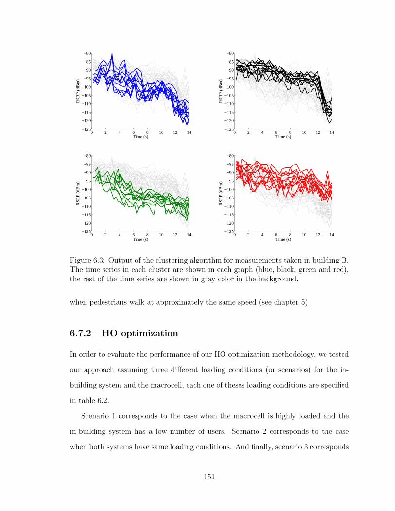
0 2 4 6 8 10 12 14−125

−120

−115

−110

−105

−100

−95

−90

−85

−80

Time (s)

RS

RP

(dB

m)

0 2 4 6 8 10 12 14−125

−120

−115

−110

−105

−100

−95

−90

−85

−80

Time (s)

RS

RP

(dB

m)

0 2 4 6 8 10 12 14−125

−120

−115

−110

−105

−100

−95

−90

−85

−80

Time (s)

RS

RP

(dB

m)

0 2 4 6 8 10 12 14−125

−120

−115

−110

−105

−100

−95

−90

−85

−80

Time (s)

RS

RP

(dB

m)

Figure 6.3: Output of the clustering algorithm for measurements taken in building B.The time series in each cluster are shown in each graph (blue, black, green and red),the rest of the time series are shown in gray color in the background.

when pedestrians walk at approximately the same speed (see chapter 5).

6.7.2 HO optimization

In order to evaluate the performance of our HO optimization methodology, we tested

our approach assuming three different loading conditions (or scenarios) for the in-

building system and the macrocell, each one of theses loading conditions are specified

in table 6.2.

Scenario 1 corresponds to the case when the macrocell is highly loaded and the

in-building system has a low number of users. Scenario 2 corresponds to the case

when both systems have same loading conditions. And finally, scenario 3 corresponds

151

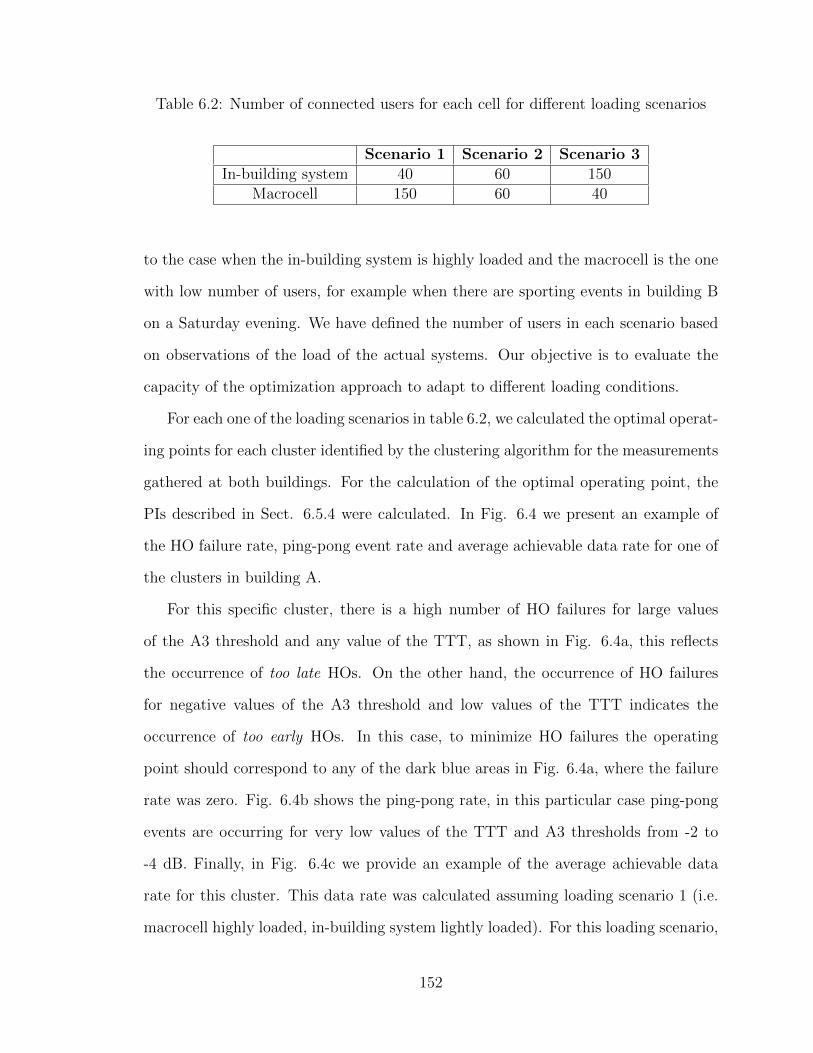
Table 6.2: Number of connected users for each cell for different loading scenarios

Scenario 1 Scenario 2 Scenario 3In-building system 40 60 150

Macrocell 150 60 40

to the case when the in-building system is highly loaded and the macrocell is the one

with low number of users, for example when there are sporting events in building B

on a Saturday evening. We have defined the number of users in each scenario based

on observations of the load of the actual systems. Our objective is to evaluate the

capacity of the optimization approach to adapt to different loading conditions.

For each one of the loading scenarios in table 6.2, we calculated the optimal operat-

ing points for each cluster identified by the clustering algorithm for the measurements

gathered at both buildings. For the calculation of the optimal operating point, the

PIs described in Sect. 6.5.4 were calculated. In Fig. 6.4 we present an example of

the HO failure rate, ping-pong event rate and average achievable data rate for one of

the clusters in building A.

For this specific cluster, there is a high number of HO failures for large values

of the A3 threshold and any value of the TTT, as shown in Fig. 6.4a, this reflects

the occurrence of too late HOs. On the other hand, the occurrence of HO failures

for negative values of the A3 threshold and low values of the TTT indicates the

occurrence of too early HOs. In this case, to minimize HO failures the operating

point should correspond to any of the dark blue areas in Fig. 6.4a, where the failure

rate was zero. Fig. 6.4b shows the ping-pong rate, in this particular case ping-pong

events are occurring for very low values of the TTT and A3 thresholds from -2 to

-4 dB. Finally, in Fig. 6.4c we provide an example of the average achievable data

rate for this cluster. This data rate was calculated assuming loading scenario 1 (i.e.

macrocell highly loaded, in-building system lightly loaded). For this loading scenario,

152

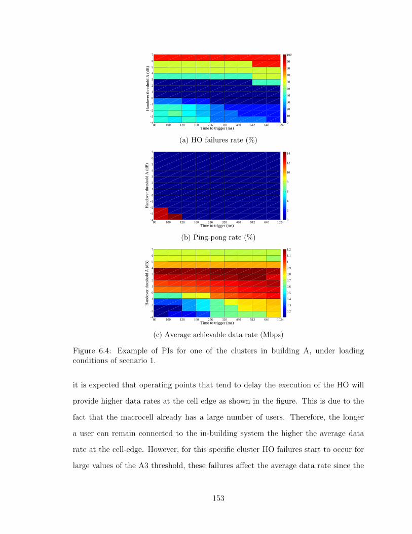
80 100 128 160 256 320 480 512 640 1024−4

−3

−2

−1

0

1

2

3

4

5

6

7

Time to trigger (ms)

Han

dove

r th

resh

old

A (

dB)

0

10

20

30

40

50

60

70

80

90

100

(a) HO failures rate (%)

80 100 128 160 256 320 480 512 640 1024−4

−3

−2

−1

0

1

2

3

4

5

6

7

Time to trigger (ms)

Han

dove

r th

resh

old

A (

dB)

0

2

4

6

8

10

12

14

(b) Ping-pong rate (%)

80 100 128 160 256 320 480 512 640 1024−4

−3

−2

−1

0

1

2

3

4

5

6

7

Time to trigger (ms)

Han

dove

r th

resh

old

A (

dB)

0.2

0.3

0.4

0.5

0.6

0.7

0.8

0.9

1

1.1

1.2

(c) Average achievable data rate (Mbps)

Figure 6.4: Example of PIs for one of the clusters in building A, under loadingconditions of scenario 1.

it is expected that operating points that tend to delay the execution of the HO will

provide higher data rates at the cell edge as shown in the figure. This is due to the

fact that the macrocell already has a large number of users. Therefore, the longer

a user can remain connected to the in-building system the higher the average data

rate at the cell-edge. However, for this specific cluster HO failures start to occur for

large values of the A3 threshold, these failures affect the average data rate since the

153

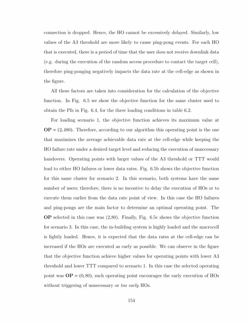
connection is dropped. Hence, the HO cannot be excessively delayed. Similarly, low

values of the A3 threshold are more likely to cause ping-pong events. For each HO

that is executed, there is a period of time that the user does not receive downlink data

(e.g. during the execution of the random access procedure to contact the target cell),

therefore ping-ponging negatively impacts the data rate at the cell-edge as shown in

the figure.

All these factors are taken into consideration for the calculation of the objective

function. In Fig. 6.5 we show the objective function for the same cluster used to

obtain the PIs in Fig. 6.4, for the three loading conditions in table 6.2.

For loading scenario 1, the objective function achieves its maximum value at

OP = (2, 480). Therefore, according to our algorithm this operating point is the one

that maximizes the average achievable data rate at the cell-edge while keeping the

HO failure rate under a desired target level and reducing the execution of unnecessary

handovers. Operating points with larger values of the A3 threshold or TTT would

lead to either HO failures or lower data rates. Fig. 6.5b shows the objective function

for this same cluster for scenario 2. In this scenario, both systems have the same

number of users; therefore, there is no incentive to delay the execution of HOs or to

execute them earlier from the data rate point of view. In this case the HO failures

and ping-pongs are the main factor to determine an optimal operating point. The

OP selected in this case was (2,80). Finally, Fig. 6.5c shows the objective function

for scenario 3. In this case, the in-building system is highly loaded and the macrocell

is lightly loaded. Hence, it is expected that the data rates at the cell-edge can be

increased if the HOs are executed as early as possible. We can observe in the figure

that the objective function achieve higher values for operating points with lower A3

threshold and lower TTT compared to scenario 1. In this case the selected operating

point was OP = (0, 80), such operating point encourages the early execution of HOs

without triggering of unnecessary or too early HOs.

154

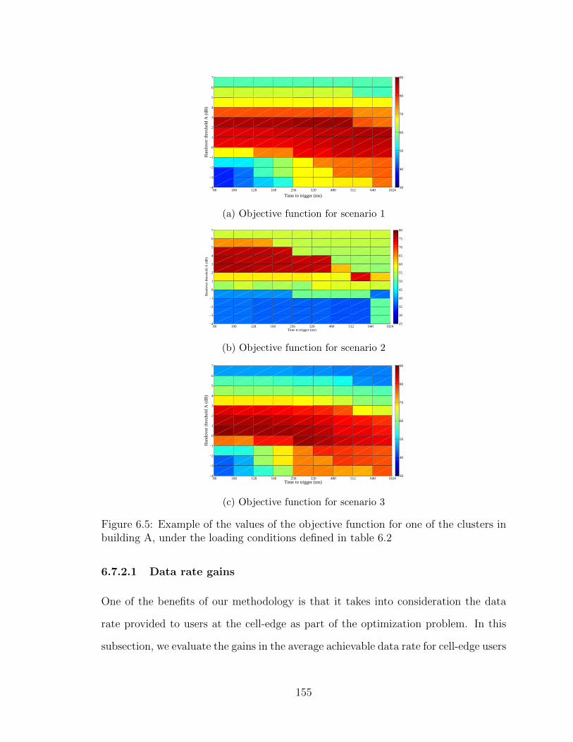
80 100 128 160 256 320 480 512 640 1024−4

−3

−2

−1

0

1

2

3

4

5

6

7

Time to trigger (ms)

Han

dove

r th

resh

old

A (

dB)

30

40

50

60

70

80

90

(a) Objective function for scenario 1

80 100 128 160 256 320 480 512 640 1024−4

−3

−2

−1

0

1

2

3

4

5

6

7

Time to trigger (ms)

Han

dove

r th

resh

old

A (

dB)

25

30

35

40

45

50

55

60

65

70

75

80

(b) Objective function for scenario 2

80 100 128 160 256 320 480 512 640 1024−4

−3

−2

−1

0

1

2

3

4

5

6

7

Time to trigger (ms)

Han

dove

r th

resh

old

A (

dB)

30

40

50

60

70

80

90

(c) Objective function for scenario 3

Figure 6.5: Example of the values of the objective function for one of the clusters inbuilding A, under the loading conditions defined in table 6.2

6.7.2.1 Data rate gains

One of the benefits of our methodology is that it takes into consideration the data

rate provided to users at the cell-edge as part of the optimization problem. In this

subsection, we evaluate the gains in the average achievable data rate for cell-edge users

155

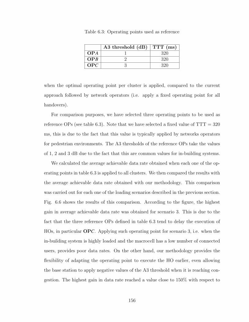
Table 6.3: Operating points used as reference

A3 threshold (dB) TTT (ms)OPA 1 320OPB 2 320OPC 3 320

when the optimal operating point per cluster is applied, compared to the current

approach followed by network operators (i.e. apply a fixed operating point for all

handovers).

For comparison purposes, we have selected three operating points to be used as

reference OPs (see table 6.3). Note that we have selected a fixed value of TTT = 320

ms, this is due to the fact that this value is typically applied by networks operators

for pedestrian environments. The A3 thresholds of the reference OPs take the values

of 1, 2 and 3 dB due to the fact that this are common values for in-building systems.

We calculated the average achievable data rate obtained when each one of the op-

erating points in table 6.3 is applied to all clusters. We then compared the results with

the average achievable data rate obtained with our methodology. This comparison

was carried out for each one of the loading scenarios described in the previous section.

Fig. 6.6 shows the results of this comparison. According to the figure, the highest

gain in average achievable data rate was obtained for scenario 3. This is due to the

fact that the three reference OPs defined in table 6.3 tend to delay the execution of

HOs, in particular OPC. Applying such operating point for scenario 3, i.e. when the

in-building system is highly loaded and the macrocell has a low number of connected

users, provides poor data rates. On the other hand, our methodology provides the

flexibility of adapting the operating point to execute the HO earlier, even allowing

the base station to apply negative values of the A3 threshold when it is reaching con-

gestion. The highest gain in data rate reached a value close to 150% with respect to

156

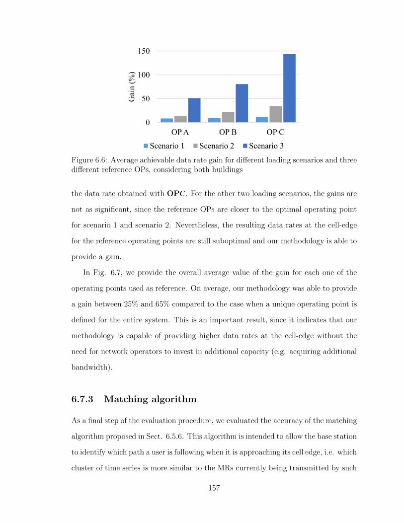
0

50

100

150

OP A OP B OP CG

ain

(%

)

Scenario 1 Scenario 2 Scenario 3

Figure 6.6: Average achievable data rate gain for different loading scenarios and threedifferent reference OPs, considering both buildings

the data rate obtained with OPC. For the other two loading scenarios, the gains are

not as significant, since the reference OPs are closer to the optimal operating point

for scenario 1 and scenario 2. Nevertheless, the resulting data rates at the cell-edge

for the reference operating points are still suboptimal and our methodology is able to

provide a gain.

In Fig. 6.7, we provide the overall average value of the gain for each one of the

operating points used as reference. On average, our methodology was able to provide

a gain between 25% and 65% compared to the case when a unique operating point is

defined for the entire system. This is an important result, since it indicates that our

methodology is capable of providing higher data rates at the cell-edge without the

need for network operators to invest in additional capacity (e.g. acquiring additional

bandwidth).

6.7.3 Matching algorithm

As a final step of the evaluation procedure, we evaluated the accuracy of the matching

algorithm proposed in Sect. 6.5.6. This algorithm is intended to allow the base station

to identify which path a user is following when it is approaching its cell edge, i.e. which

cluster of time series is more similar to the MRs currently being transmitted by such

157

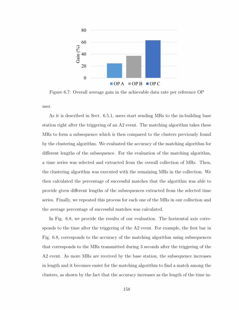
0

20

40

60

80

Gai

n (

%)

OP A OP B OP C

Figure 6.7: Overall average gain in the achievable data rate per reference OP

user.

As it is described in Sect. 6.5.1, users start sending MRs to the in-building base

station right after the triggering of an A2 event. The matching algorithm takes these

MRs to form a subsequence which is then compared to the clusters previously found

by the clustering algorithm. We evaluated the accuracy of the matching algorithm for

different lengths of the subsequence. For the evaluation of the matching algorithm,

a time series was selected and extracted from the overall collection of MRs. Then,

the clustering algorithm was executed with the remaining MRs in the collection. We

then calculated the percentage of successful matches that the algorithm was able to

provide given different lengths of the subsequences extracted from the selected time

series. Finally, we repeated this process for each one of the MRs in our collection and

the average percentage of successful matches was calculated.

In Fig. 6.8, we provide the results of our evaluation. The horizontal axis corre-

sponds to the time after the triggering of the A2 event. For example, the first bar in

Fig. 6.8, corresponds to the accuracy of the matching algorithm using subsequences

that corresponds to the MRs transmitted during 3 seconds after the triggering of the

A2 event. As more MRs are received by the base station, the subsequence increases

in length and it becomes easier for the matching algorithm to find a match among the

clusters, as shown by the fact that the accuracy increases as the length of the time in-

158

0

20

40

60

80

100

3 3.5 4 4.5 5 5.5A

ccu

racy

(%

)Time from the triggering of A2 event(s)

Figure 6.8: Accuracy of the matching algorithm vs the time after the triggering ofthe A2 event

creases. Based on these results, at least 4 seconds of transmitted MRs from each user

approaching the cell-edge are required to reach a matching accuracy above 90%. The

number of MRs required to reach this accuracy depends on the frequency of trans-

mission of the MRs. In our case, one MR was transmitted every 300 ms; hence, on

average 14 MRs were needed to reach a matching accuracy above 90%. The accuracy

can reach a value close to 100% when this time increases to 5.5 seconds.

6.8 Summary

In this chapter we proposed a methodology that provides in-building base stations

with the flexibility to customize HO parameters to specific radio frequency conditions

at the cell-edge for different loading scenarios. We propose the use of machine learning

and data mining techniques to allow the base stations to autonomously learn and

identify characteristic patterns in the RSRP values as users approach the cell-edge,

and apply optimal HO parameters for each case. Our results show that our clustering

algorithm based on shapelets and wavelet decomposition is capable of accurately

identifying patterns in RSRP measurements reports collected from operational LTE

in-building systems deployed in a university campus. Furthermore, our approach

159

was able to optimize HO parameters by jointly considering loading conditions of the

serving and target cell as well as the RF conditions of the cell edge captured in

each cluster. With the application of the optimal HO parameters per cluster, the

in-building base station was able to maximize data rates, keep HO failure rate under

a desired target and reduce the triggering of unnecessary HOs. Our approach was

able to provide average data rate gains between 25% and 65%. Depending on the

operating point used as reference, the data rate gain can reach a value close to 150%

for certain loading conditions. These results support the fact that this approach is

a viable option to increase spectral efficiency at the cell edge while guarantying the

continuity of service when HOs are executed.

160

Chapter 7

Conclusions

7.1 Summary

Heterogeneous networks are becoming the preferred choice of network operators to

meet the ever increasing demand of data traffic in mobile networks. Such increase

in demand is fueled by the development of bandwidth intensive applications and a

growing number of mobile devices that include smartphones, tablets, laptops and

wearables. The multi-tier network topology in HetNets brings a new series of impor-

tant challenges for network operators. There is a need to increase the understanding

of the operation of these systems and develop new techniques to properly plan, design

and optimize HetNets, since traditional practices applied for macrocell-only networks

do not provide optimal results in this type of network. These new techniques should

focus on the efficient use of resources during network planning, reducing costs of de-

ployments, and facilitating the configuration and maintenance of HetNets. Especially

with the massive increase in network densification expected in the following years, a

situation that will significantly increase the complexity of the network. The research

work described in this thesis has the overall objective of expanding the understanding

and exploring novel solutions to some of these new challenges. We now proceed to

summarize the main contributions of this thesis.

In Chapter 2 we proposed two novel tuning methods, a semi-global and a local

method, to improve the accuracy of a site-specific path loss prediction model based

on the Uniform Theory of Diffraction (UTD). Such site-specific model is intended

to be applied during the planning and design stages of deployments involving out-

161

door microcells. The purpose of these tuning methods is to adaptively adjust the

propagation model parameters according to the propagation conditions at different

locations of the area of interest. As a result, the model parameters are optimized

for different areas of the map. With the traditional tuning methodologies proposed

in the literature, only a single set of model parameters is calculated and applied to

the entire area of interest (i.e. global tuning). We demonstrated that a global tun-

ing procedure is not capable of properly adjusting the path loss model to the actual

physical environment. We showed that tuning the model locally is the best approach

to minimize path loss prediction errors when physical measurements from walk and

drive tests are available. According to our experimental evaluation, tuning the model

locally provides a significant reduction of the overall mean absolute error between

measurements and path loss estimations, such reduction is close to 35% compared

to the case when the model is not tuned. Additionally, the local tuning provided a

substantial reduction of the mean absolute error for the vast majority of our experi-

mental observations. According to the cumulative distribution of the mean absolute

error (MAE), the untuned model presented up to 250% higher MAE compared to

the locally tuned model for the 80th percentile of the observations. In general, the

local tuning procedure outperformed the global and the semi-global tuning methods

for any percentile, for any size of the training set and for any location of the test

transmitter.

The results of this study show that a local tuning of the path loss prediction model

provides a practical and flexible way to optimize the parameters of the propagation

model, since prediction errors are corrected based on very specific local propagation

conditions. Furthermore, from a practical point of view, it is important for network

operators to minimize the time and resources spent collecting walk and drive test

data. Based on our observations, the accuracy of the path loss predictions decrease as

the propagation path becomes more complex. This observation can then be applied

162

to make the collection of measured data more efficient (i.e. data collection efforts

should be concentrated in gathering measurements in areas where it is expected that

the prediction model will be inaccurate). Our local tuning procedure, combined with

the semi-global tuning approach, are aimed at taking advantage of a limited set of

measured data gathered specifically at those strategic locations where the tuning of

the model is most needed.

In Chapter 3, we described and validated an LTE/LTE-A downlink simulator

capable of modeling the walk/speed tests carried out by network operators during

the planning stage of a new cell site. The simulation tool incorporates a realistic

traffic model based on QoS requirements, such requirements are defined according to

the type of traffic that a specific user demands. The simulator was validated with

measurement data collected from a live LTE network, with emphasis on cell-edge

regions. The validation of the simulation tool was focused on two main aspects: the

analysis and modeling of the user experience as mobiles move towards the cell-edge,

and secondly the effects of different loading conditions on the user experience. We

demonstrated that classifying the traffic demand in categories (e.g. according to the

QoS requirements), leads to a substantially more accurate estimation of downlink data

rates as users move; in particular, as users approach the cell-edge and are handed over

to a neighboring cell. We were able to show a superior performance in the modeling

of the walk/speed tests when our QoS traffic model was applied as opposed to the

traditional full buffer model. Our methodology to model walk/speed tests was able

to capture the actual behavior of the data rate during a handover subject to different

loading conditions, as oppose to the full buffer model that tends to significantly under-

estimate the downlink data rate. With our QoS-aware traffic model, we obtained up

to 86% higher accuracy is data rate estimations compared to the traditional full-buffer

model.

In Chapter 4, we proposed a novel and practical distributed load balancing al-

163

gorithm. The main objective of the algorithm was to provide a fair distribution of

the load among base stations in a HetNet. With our algorithm, each base station

can solve locally a load-aware utility maximization problem. Such problem is solved

based on the information of the current eNB’s load level, resource scheduling and

SINR conditions of its associated users. By solving the utility maximization problem

locally, an overloaded base station can determine which users are negatively impact-

ing its sum of the utility, those users are then candidates to be transferred to other

base stations with spare capacity via load-aware handover procedures. The algorithm

was formulated with the objective of minimizing the required amount of coordination

and exchange of information among base stations (e.g. handover triggering), because

an excessive exchange of signaling messages is undesired and leads to an increase in

power consumption. The algorithm was evaluated through a comparative analysis

with two other iterative near-optimal load balancing algorithms based on convex op-

timization. We evaluated the effectiveness of these algorithms considering a typical

two-tier HetNet deployment subject to a realistic traffic distribution. We were able to

show that our algorithm provided similar offloading of users from the macrocell and

almost identical gains in downlink data rates compared to the other near-optimal al-

gorithms. With the main advantage that our algorithm was substantially less complex

and required a minimal amount of exchange of messages among base stations. This

leads to lower levels of coordination and lower impact on the signaling load of the net-

work. Additionally, by reducing the amount of signaling messages exchanged among

base stations, their power consumption is not significantly impacted, as opposed to

the case when the other two load balancing algorithms are applied.

In Chapter 5, we proposed a novel methodology to classify mobile users according

to their trajectory as they leave the coverage area of an in-building system. The

methodology is based on a time series clustering algorithm and its main objective is

to provide indoor base stations with the capability to discover and learn the radio

164

frequency conditions that their users are subject to when they approach the cell-edge,

without actually knowing the physical location of the mobile devices. The key insight

of the approach is to identify similarities among the sets of received signal strength

measurements reported by each user as part of the handover process in LTE systems.

The measurement reports from users following similar trajectories present high levels

of correlation; therefore, this information can be used to determine characteristic pat-

terns in the measurement reports that can be applied to classify users according to

their trajectory. Our methodology is based on a novel time series clustering algorithm

based on shape similarity to identify and classify the characteristic patterns captured

in the reported measurements. We proposed to apply a shape-based technique called

unsupervised-shapelets combined with a multi-resolution wavelet decomposition anal-

ysis. Our simulations considered an LTE network consisting of a macrocell and an in-

door microcell. Our clustering algorithm based on unsupervised-shapelets and multi-

resolution wavelet decomposition (SW) provided superior performance compared to

a DFT-based clustering algorithm. Our algorithm SW was able to provide clustering

results close to 12% more accurate and up to 75% better quality of clusters. On

average, with our methodology we were able to correctly identify and classify the

measurements reports with an accuracy of 92%. This methodology is intended to

increase the capacity of base stations to autonomously learn and discover the radio

frequency conditions of their irregular cell-edge. Furthermore, the methodology is an

essential component of the handover optimization strategy proposed in Chapter 6.

In Chapter 6 we proposed a novel methodology to optimize handover parameters

for in-building systems, with the objective of minimizing handover failures and the

triggering of unnecessary handovers, while maximizing the QoS provided to users ap-

proaching the cell-edge. In the context of self-optimizing networks, with the proposed

methodology we intend to provide base stations with the means to automatically de-

termine suitable handover parameters for each user, such that the continuity of service

165

is guaranteed while maximizing the downlink data rates provided to the user. In other

words, the methodology allows indoor base stations to customize handover parameters

to provide an optimal service at the user level. The key insight behind our methodol-

ogy is the adjustment of the handover parameters (time-to-trigger and received signal

level threshold) based on the knowledge that base stations are able to learn and dis-

cover regarding the RF conditions of their cell-edge. Such knowledge is obtained with

the application of the time series clustering algorithm proposed in Chapter 5. The

handover parameters are optimized by jointly considering the levels of interference at

the cell-edge and the load levels of both, the target and serving cells. An objective

function is defined in terms of four key performance indicators: the handover failure

rate, handover ping-pong rate, number of handovers triggered and the average achiev-

able data rate for each cluster of users following a similar trajectory. Finally, the set

of handover parameters that maximizes the objective function is determined for each

cluster. Based on our experimental results, our approach was able to provide average

data rate gains between 25% and 65%. Depending on the operating point used as

reference, the data rate gain can even reach a value close to 150% for certain loading

conditions. These results support the fact that this approach is a viable option to

increase spectral efficiency at the cell-edge while guarantying the continuity of service

when handovers are executed. To the best of our knowledge, a similar methodology

for the optimization of handover parameters has not been proposed in the literature.

7.2 Future research directions

This thesis has investigated and explored solutions to some of the key challenges in

HetNets, covering aspects from the planning stage to the self-optimization of handover

parameters. Given the fact that network densification will continue to increase in the

following years, it is expected that there will be a need to continue the investigation

166

about the operation of HetNets.

The current tendency among network operators is to bring the base stations closer

to the users, this means that a dramatic increase in the number of indoor base stations

is expected to occur. Therefore, the work proposed in this thesis regarding the tuning

of site-specific models can be extended to include the case of propagation of signals in

indoor environments, particularly in multi-story buildings. Especially considering the

fact that millimeter wave communications (mmWave) combined with massive MIMO

appears to be the next step to deal with spectrum scarcity [96–98].

Additionally, the load balancing problem in HetNets is still not fully understood.

Most of the current load balancing algorithms tend to concentrate on optimizing cell

association with respect to the downlink only. Nowadays, mobile users tend to upload

media content very often as part of their social media activities; therefore, a good

user experience also involves a reliable and fast uplink connection. Hence, further

investigation is required to define suitable cell association rules and load balancing

algorithms that jointly considers both uplink and downlink in co-channel scenarios.

Even considering the case when one base station provides the downlink connection and

other base station is in charge of the uplink connection, in the context of Coordinated

Multi-point communications (CoMP) [99,100].

The role of SON functionalities will become essential for network operators in order

to efficiently deal with a large number of base stations handling a massive number

of users. Our methodology to optimize handover parameters is a good example of

the current tendency in this area, where some of the operational parameters can

be customized at the user level. The application of machine learning techniques

will become a fundamental component in the design and development of new SON

functionalities for the next generation of mobile wireless systems [101]. For example,

the ability to dynamically coordinate the use of non-contiguous spectrum allocations

according to loading conditions in a cooperative way among tiers in HetNets. In

167

general, the paradigm behind traditional SON functionalities has to change from the

current observe and act perspective to a more proactive approach, where predictive

functionalities will be essential, and all of this while keeping energy efficiency as a

one of the primary restrictions.

168

References

[1] 3GPP. (2016, Nov.) Evolved Universal Terrestrial Radio Access Network

(E-UTRAN) - Physical layer procedures. 3GPP. [Online]. Available:

http://www.3gpp.org/dynareport/36-series.htm

[2] Cisco, “Cisco Visual Networking Index: Global Mobile Data Traffic Forecast

Update, 2015-2020,” White paper, Feb. 2016.

[3] D. Ngo and T. Le-Ngoc, Architectures and Interference Management for Small-

Cell Networks. Springer International Publishing, 2014, ch. 1.

[4] S. Brueck, “Heterogeneous networks in LTE-Advanced,” in 2011 8th Interna-

tional Symposium on Wireless Communication Systems (ISWCS), 2011, pp.

171–175.

[5] J. G. Andrews, “Seven ways that HetNets are a cellular paradigm shift,” IEEE

Communications Magazine, vol. 51, no. 3, pp. 136–144, 2013.

[6] V. Chandrasekhar, J. G. Andrews, and A. Gatherer, “Femtocell networks: a

survey,” IEEE Communications Magazine, vol. 46, no. 9, pp. 59–67, Sep. 2008.

[7] D. Liu, L. Wang, Y. Chen, M. Elkashlan, K.-K. Wong, R. Schober, and

L. Hanzo, “User Association in 5G Networks: A Survey and an Outlook,” IEEE

Communications Surveys & Tutorials, vol. 18, no. 2, pp. 1018–1044, 2016.

[8] Y.-C. Wang and C.-A. Chuang, “Efficient eNB deployment strategy for hetero-

geneous cells in 4G LTE systems,” Computer Networks, vol. 79, pp. 297–312,

Mar. 2015.

[9] M. Hata, “Empirical formula for propagation loss in land mobile radio services,”

IEEE Transactions on Vehicular Technology, vol. 29, no. 3, pp. 317–325, Aug.

1980.

[10] Y. Okumura, E. Ohmori, T. Kawano, and K. Fukuda, “Field strength and its

variability in VHF and UHF land-mobile radio service,” Review of the Electrical

Communication Laboratory, vol. 16, no. 9-10, pp. 825–873, 1968.

[11] M. N. Lustgarten and J. A. Madison, “An Empirical Propagation Model (EPM-

73),” IEEE Transactions on Electromagnetic Compatibility, vol. 19, no. 3, pp.

301–309, Aug. 1977.

[12] N. Noe, F. Gaudaire, and D. B. Lo, “Estimating and reducing uncertainties

in ray-tracing techniques for electromagnetic field exposure in urban areas,” in

Topical Conference on Antennas and Propagation in Wireless Communications

(APWC). IEEE, 2013, pp. 652–655.

[13] K. Heiska and A. Kangas, “Microcell propagation model for network planning,”

in Seventh IEEE International Symposium on Personal, Indoor and Mobile Ra-

dio Communications, vol. 1. IEEE, Oct. 1996, pp. 148–152 vol.1.

[14] A. Navarro, D. Guevara, N. Cardona, and J. Lopez, “Measurement-based ray-

tracing models calibration in urban environments,” in Proceedings of the 2012

IEEE International Symposium on Antennas and Propagation. IEEE, Jul.

2012, pp. 1–2.

[15] J. Jemai and T. Kurner, “Towards a Performance Boundary in Calibrating

Indoor Ray Tracing Models,” EURASIP Journal on Wireless Communications

and Networking, vol. 2009, no. 1, pp. 1–8, 2009.

170

[16] B. Y. Hanci and I. H. Cavdar, “Mobile radio propagation measurements and

tuning the path loss model in urban areas at GSM-900 band in Istanbul-

Turkey,” in Vehicular Technology Conference (VTC-Fall), vol. 1, 2004, pp.

139–143 Vol. 1.

[17] L. Juan-Llacer, L. Ramos, and N. Cardona, “Application of some theoretical

models for coverage prediction in macrocell urban environments,” IEEE Trans-

actions on Vehicular Technology, vol. 48, no. 5, pp. 1463–1468, Sep. 1999.

[18] A. Salieto, G. Roig, D. Gomez-Barquero, and N. Cardona, “Radio propagation

models for DVB-H networks,” in Proceedings of the Fourth European Conference

on Antennas and Propagation. IEEE, Apr. 2010, pp. 1–5.

[19] L. Klozar and J. Prokopec, “Propagation path loss models for mobile commu-

nication,” in 21st IEEE International Conference Radioelektronika, Apr. 2011,

pp. 1–4.

[20] A. Tahat and M. Taha, “Statistical tuning of Walfisch-Ikegami propagation

model using Particle Swarm Optimization,” in 2012 19th IEEE Symposium on

Communications and Vehicular Technology in the Benelux (SCVT). IEEE,

Nov. 2012, pp. 1–6.

[21] D. Ambawade, D. Karia, T. Potdar, B. K. Lande, R. D. Daruwala, and A. Shah,

“Statistical Tuning of Walfisch-Ikegami Model in Urban and Suburban En-

vironments,” in 2010 Fourth Asia International Conference on Mathemati-

cal/Analytical Modelling and Computer Simulation. IEEE, May 2010, pp.

538–543.

[22] E. O. Rozal and E. G. Pelaes, “Statistical adjustment of Walfisch-Ikegami model

based in urban propagation measurements,” in International Conference on

Microwave and Optoelectronics. IEEE, Oct. 2007, pp. 584–588.

171

[23] L. Subrt and P. Pechac, “Advanced 3D indoor propagation model: calibra-

tion and implementation,” EURASIP Journal on Wireless Communications

and Networking, vol. 2011, no. 1, pp. 1–10, 2011.

[24] D. Castro-Hernandez and R. Paranjape, “Estimation of coverage areas in mi-

crocells,” in 2013 IEEE International Conference on Advanced Networks and

Telecommunications Systems (ANTS). IEEE, Dec. 2013, pp. 1–6.

[25] H. S. Dhillon, R. K. Ganti, F. Baccelli, and J. G. Andrews, “Modeling and

Analysis of K-Tier Downlink Heterogeneous Cellular Networks,” IEEE Journal

on Selected Areas in Communications, vol. 30, no. 3, pp. 550–560, Apr. 2012.

[26] S. Mukherjee, “Distribution of Downlink SINR in Heterogeneous Cellular Net-

works,” IEEE Journal on Selected Areas in Communications, vol. 30, no. 3, pp.

575–585, Apr. 2012.

[27] Q. Ye, B. Rong, Y. Chen, M. Al-Shalash, C. Caramanis, and J. G. Andrews,

“User Association for Load Balancing in Heterogeneous Cellular Networks,”

IEEE Transactions on Wireless Communications, vol. 12, no. 6, pp. 2706–2716,

Jun. 2013.

[28] K. Shen and W. Yu, “Distributed Pricing-Based User Association for Downlink

Heterogeneous Cellular Networks,” IEEE Journal on Selected Areas in Com-

munications, vol. 32, no. 6, pp. 1100–1113, Jun. 2014.

[29] M. Simsek, M. Bennis, and I. Guvenc, “Mobility management in HetNets: a

learning-based perspective,” EURASIP Journal on Wireless Communications

and Networking, no. 26, 2015.

172

[30] A. Damnjanovic, J. Montojo, J. Cho, H. Ji, J. Yang, and P. Zong, “UE’s role

in LTE advanced heterogeneous networks,” IEEE Communications Magazine,

vol. 50, no. 2, pp. 164–176, Feb. 2012.

[31] L. Hu, L. L. Sanchez, M. Maternia, I. Kovacs, B. Vejlgaard, P. Mogensen,

and H. Taoka, “Heterogeneous LTE-Advanced Network Expansion for 1000x

Capacity,” in Vehicular Technology Conference (VTC Spring). IEEE, Jun.

2013, pp. 1–5.

[32] O. Galinina, S. Andreev, M. Gerasimenko, Y. Koucheryavy, N. Himayat, S.-P.

Yeh, and S. Talwar, “Capturing Spatial Randomness of Heterogeneous Cel-

lular/WLAN Deployments With Dynamic Traffic,” IEEE Journal on Selected

Areas in Communications, vol. 32, no. 6, pp. 1083–1099, Jun. 2014.

[33] J. G. Andrews, S. Singh, Q. Ye, X. Lin, and H. S. Dhillon, “An overview

of load balancing in hetnets: old myths and open problems,” IEEE Wireless

Communications, vol. 21, no. 2, pp. 18–25, Apr. 2014.

[34] 3GPP, “Evolved Universal Terrestrial Radio Access Network (E-

UTRAN),” Technical Standard, 3GPP, 2016. [Online]. Available:

http://www.3gpp.org/dynareport/36-series.htm

[35] I. Guvenc, “Capacity and Fairness Analysis of Heterogeneous Networks with

Range Expansion and Interference Coordination,” IEEE Communications Let-

ters, vol. 15, no. 10, pp. 1084–1087, Oct. 2011.

[36] S. Mishra, A. Sengupta, and S. R. Murthy, “Enhancing the performance of

HetNets via linear regression estimation of Range Expansion Bias,” in IEEE

International Conference on Networks. IEEE, Dec. 2013, pp. 1–6.

173

[37] I. Siomina and D. Yuan, “Load balancing in heterogeneous LTE: Range opti-

mization via cell offset and load-coupling characterization,” in IEEE Interna-

tional Conference on Communications. IEEE, Jun. 2012, pp. 1357–1361.

[38] P. Tian, H. Tian, J. Zhu, L. Chen, and X. She, “An adaptive bias configuration

strategy for Range Extension in LTE-Advanced Heterogeneous Networks,” in

IET International Conference on Communication Technology and Application.

IET, Oct. 2011, pp. 336–340.

[39] K. Kikuchi and H. Otsuka, “Proposal of adaptive control CRE in heterogeneous

networks,” in IEEE International Symposium on Personal, Indoor and Mobile

Radio Communications. IEEE, 2012, pp. 910–914.

[40] B. A. Yasir, G. Su, and N. Bachache, “Range expansion for pico cell in hetero-

geneous LTE - A cellular networks,” in International Conference on Computer

Science and Network Technology. IEEE, Dec. 2012, pp. 1235–1240.

[41] Y. Sun, T. Deng, Y. Fang, M. Wang, and Y. Wu, “A method for pico-specific

upper bound CRE bias setting in HetNet,” in Wireless Communications and

Networking Conference Workshops (WCNCW). IEEE, Apr. 2013, pp. 80–84.

[42] L. Jorguseski, A. Pais, F. Gunnarsson, A. Centonza, and C. Willcock, “Self-

organizing networks in 3GPP: standardization and future trends,” IEEE Com-

munications Magazine, vol. 52, no. 12, pp. 28–34, Dec. 2014.

[43] M. Peng, D. Liang, Y. Wei, J. Li, and H.-H. Chen, “Self-configuration and

self-optimization in LTE-advanced heterogeneous networks,” IEEE Communi-

cations Magazine, vol. 51, no. 5, pp. 36–45, May 2013.

174

[44] D. Aziz, A. Ambrosy, L. T. W. Ho, L. Ewe, M. Gruber, and H. Bakker, “Au-

tonomous neighbor relation detection and handover optimization in LTE,” Bell

Labs Technical Journal, vol. 15, no. 3, pp. 63–83, Dec. 2010.

[45] Y. Watanabe, Y. Matsunaga, K. Kobayashi, H. Sugahara, and K. Hamabe,

“Dynamic Neighbor Cell List Management for Handover Optimization in LTE,”

in Vehicular Technology Conference (VTC Spring). IEEE, May 2011, pp. 1–5.

[46] Z. Guohua, P. Legg, and G. Hui, “A network controlled handover mechanism

and its optimization in LTE heterogeneous networks,” in 2013 IEEE Wireless

Communications and Networking Conference (WCNC). IEEE, Apr. 2013, pp.

1915–1919.

[47] T. Jansen, I. Balan, J. Turk, I. Moerman, and T. Kurner, “Handover Param-

eter Optimization in LTE Self-Organizing Networks,” in Vehicular Technology

Conference Fall (VTC-Fall). IEEE, 2010, pp. 1–5.

[48] G. Hui and P. Legg, “Soft Metric Assisted Mobility Robustness Optimization

in LTE Networks,” in International Symposium on Wireless Communication

Systems. IEEE, Aug. 2012, pp. 1–5.

[49] L. Ewe and H. Bakker, “Base station distributed handover optimization in

LTE self-organizing networks,” in IEEE International Symposium on Personal,

Indoor and Mobile Radio Communications. IEEE, 2011, pp. 243–247.

[50] K. Kitagawa, T. Komine, T. Yamamoto, and S. Konishi, “A handover opti-

mization algorithm with mobility robustness for LTE systems,” in IEEE Inter-

national Symposium on Personal, Indoor and Mobile Radio Communications.

IEEE, 2011, pp. 1647–1651.

175

[51] G. Zhou and P. Legg, “An Evolved Mobility Robustness Optimization Algo-

rithm for LTE Heterogeneous Networks,” in Vehicular Technology Conference

(VTC Spring). IEEE, Jun. 2013, pp. 1–5.

[52] V. Capdevielle, A. Feki, and A. Fakhreddine, “Self-optimization of handover

parameters in LTE networks,” in International Symposium on Modeling & Op-

timization in Mobile, Ad Hoc & Wireless Networks. IEEE, May 2013, pp.

133–139.

[53] W. Gao, B. Jiao, G. Yang, W. Hu, L. Chi, and J. Liu, “Mobility robustness

improvement through transport parameter optimization in HetNets,” in Inter-

national Symposium on Personal, Indoor and Mobile Radio Communications.

IEEE, 2013, pp. 101–105.

[54] R. D. Hegazy and O. A. Nasr, “A user behavior based handover optimization al-

gorithm for LTE networks,” in IEEE Wireless Communications and Networking

Conference (WCNC). IEEE, Mar. 2015, pp. 1255–1260.

[55] B. Sas, K. Spaey, and C. Blondia, “A SON Function for Steering Users in

Multi-Layer LTE Networks Based on Their Mobility Behaviour,” in Vehicular

Technology Conference (VTC Spring). IEEE, May 2015, pp. 1–7.

[56] D. Castro-Hernandez and R. Paranjape, “Local tuning of a site-specific propaga-

tion path loss model for microcell environments,” Journal on Wireless Personal

Communications, 2016, DOI: 10.1007/s11277-016-3489-0.

[57] ——, “A distributed load balancing algorithm for LTE/LTE-A heterogeneous

networks,” in Wireless Communications and Networking Conference Work-

shops. IEEE, Mar. 2015, pp. 380–385.

176

[58] ——, “Comparative analysis of load balancing algorithms for LTE/LTE-A Het-

nets,” in 2015 International Conference on Wireless Communication, Vehicular

Technology, Information Theory and Aerospace and Electronic Systems Tech-

nology (Wireless VITAE). IEEE, Dec. 2015.

[59] ——, “Walk test simulator for LTE/LTE-A network planning,” in International

Telecommunications Network Strategy and Planning Symposium (NETWORKS

2016). IEEE, Sep. 2016.

[60] ——, “Classification of user trajectories in LTE HetNets using unsupervised-

shapelets and multi-resolution wavelet decomposition,” unpublished.

[61] ——, “Optimization of handover parameters for LTE/LTE-A in-building sys-

tems,” unpublished.

[62] K. R. Schaubach and N. J. Davis, “Microcellular radio-channel propagation

prediction,” IEEE Antennas and Propagation Magazine, vol. 36, no. 4, pp. 25–

34, Aug. 1994.

[63] M. Yang, S. Stavrou, and A. K. Brown, “Hybrid ray-tracing model for radio

wave propagation through periodic building structures,” IET Microwaves, An-

tennas & Propagation, vol. 5, no. 3, pp. 340–348, Feb. 2011.

[64] Y.-S. Feng, L.-X. Guo, P. Wang, and Z.-Y. Liu, “Efficient ray-tracing model

for propagation prediction for microcellular wireless communication systems,”

in International Symposium on Antennas, Propagation & EM Theory. IEEE,

Oct. 2012, pp. 432–435.

[65] Y.-K. Yoon, M.-W. Jung, and J. Kim, “Intelligent ray tracing for the propaga-

tion prediction,” in Proceedings of the 2012 IEEE International Symposium on

Antennas and Propagation. IEEE, Jul. 2012, pp. 1–2.

177

[66] F. Puggelli, G. Carluccio, and M. Albani, “A Novel Ray Tracing Algorithm for

Scenarios Comprising Pre-Ordered Multiple Planar Reflectors, Straight Wedges,

and Vertexes,” IEEE Transactions on Antennas and Propagation, vol. 62, no. 8,

pp. 4336–4341, Aug. 2014.

[67] P. Wang, L.-X. Guo, and Y.-S. Feng, “A fast ray-tracing algorithm for microcel-

lular propagation prediction models,” in International Symposium on Antennas,

Propagation & EM Theory. IEEE, Oct. 2012, pp. 436–439.

[68] V. Mohtashami and A. A. Shishegar, “Effects of inaccuracy of material permit-

tivities on ray tracing results for site- specific indoor propagation modeling,” in

Topical Conference on Antennas and Propagation in Wireless Communications.

IEEE, 2013, pp. 1172–1175.

[69] R. G. Kouyoumjian and P. H. Pathak, “A uniform geometrical theory of diffrac-

tion for an edge in a perfectly conducting surface,” Proceedings of the IEEE,

vol. 62, no. 11, pp. 1448–1461, Nov. 1974.

[70] S. Y. Tan and H. S. Tan, “A microcellular communications propagation model

based on the uniform theory of diffraction and multiple image theory,” IEEE

Transactions on Antennas and Propagation, vol. 44, no. 10, pp. 1317–1326, Oct.

1996.

[71] T. S. Rappaport, Wireless Communications: Principles and Practice (2nd Edi-

tion), 2nd ed. Prentice Hall, Jan. 2002.

[72] C. Tzaras and S. R. Saunders, “An improved heuristic UTD solution for

multiple-edge transition zone diffraction,” IEEE Transactions on Antennas and

Propagation, vol. 49, no. 12, pp. 1678–1682, Dec. 2001.

178

[73] M. B. Tabakcioglu and A. Kara, “On the Improvements in Multiple Edge Tran-

sition Zone Diffraction,” in Second European Conference on Antennas and Prop-

agation. IET, Nov. 2007, pp. 1–5.

[74] K. Rizk, R. Valenzuela, D. Chizhik, and F. Gardiol, “Application of the slope

diffraction method for urban microwave propagation prediction,” in Vehicular

Technology Conference, vol. 2. IEEE, May 1998, pp. 1150–1155 vol.2.

[75] K. Benzair, “Measurements and modelling of propagation losses through vege-

tation at 1-4 GHz,” in International Conference on Antennas and Propagation,

vol. 2. IET, Apr. 1995, pp. 54–59 vol.2.

[76] Infovista. (2016, Apr.) Mentum Planet. Infovista. [Online]. Avail-

able: http://www.infovista.com/products/Mentum-Planet-Live-RF-planning-

and-optimization

[77] iBwave. (2016, Apr.) iBwave: In-building network design tool. iBwave.

[Online]. Available: http://www.ibwave.com/

[78] M. Rupp, S. Schwarz, and M. Taranetz, The Vienna LTE-Advanced Simulators.

Singapore: Springer Singapore, 2016.

[79] C. Mehlfuhrer, J. Colom Ikuno, M. Simko, S. Schwarz, M. Wrulich, and

M. Rupp, “The Vienna LTE simulators - Enabling reproducibility in wireless

communications research,” EURASIP Journal on Advances in Signal Process-

ing, vol. 2011, no. 1, 2011.

[80] A. Ghosh, N. Mangalvedhe, R. Ratasuk, B. Mondal, M. Cudak, E. Visotsky,

T. A. Thomas, J. G. Andrews, P. Xia, H. S. Jo, H. S. Dhillon, and T. D.

Novlan, “Heterogeneous cellular networks: From theory to practice,” IEEE

Communications Magazine, vol. 50, no. 6, pp. 54–64, Jun. 2012.

179

[81] M. Kawser, N. I. B. Hamid, N. Hasan, S. Alam, and M. Rahman, “Downlink

SNR to CQI Mapping for Different Multiple Antenna Techniques in LTE,”

International Journal of Information and Electronics Engineering, vol. 2, no. 5,

pp. 756–760, 2012.

[82] B. Soret and K. I. Pedersen, “Centralized and Distributed Solutions for Fast

Muting Adaptation in LTE-Advanced HetNets,” IEEE Transactions on Vehic-

ular Technology, vol. 64, no. 1, pp. 147–158, Jan. 2015.

[83] D. Lopez-Perez, I. Guvenc, and X. Chu, “Mobility management challenges

in 3GPP heterogeneous networks,” IEEE Communications Magazine, vol. 50,

no. 12, pp. 70–78, Dec. 2012.

[84] K. Somasundaram, “Proportional Fairness in LTE-Advanced Heterogeneous

Networks with eICIC,” in Vehicular Technology Conference (VTC Fall), Sept

2013, pp. 1–6.

[85] 3GPP, “TS 36.902: Evolved Universal Terrestrial Radio Access Network (E-

UTRAN); Self-Configuring and Self-Optimizing Network (SON) Use Cases and

Solutions,” 3GPP, Tech. Rep., May 2011.

[86] J. Hills, J. Lines, E. Baranauskas, J. Mapp, and A. Bagnall, “Classification of

time series by shapelet transformation,” Data Mining and Knowledge Discovery,

vol. 28, no. 4, pp. 851–881, 2014.

[87] E. Keogh and C. A. Ratanamahatana, “Exact indexing of dynamic time warp-

ing,” Knowledge and Information Systems, vol. 7, no. 3, pp. 358–386, Mar.

2005.

[88] X. Wang, A. Mueen, H. Ding, G. Trajcevski, P. Scheuermann, and E. Keogh,

“Experimental comparison of representation methods and distance measures

180

for time series data,” Data Mining and Knowledge Discovery, vol. 26, no. 2, pp.

275–309, Feb. 2013.

[89] L. Ye and E. Keogh, “Time series shapelets: a novel technique that allows

accurate, interpretable and fast classification,” Data Mining and Knowledge

Discovery, vol. 22, no. 1-2, pp. 149–182, Jan. 2011.

[90] J. Zakaria, A. Mueen, and E. Keogh, “Clustering Time Series Using

Unsupervised-Shapelets,” in IEEE International Conference on Data Mining.

IEEE, Dec. 2012, pp. 785–794.

[91] J. Macqueen, “Some methods for classification and analysis of multivariate ob-

servations,” in 5th Berkeley Symposium on Mathematical Statistics and Proba-

bility, 1967, pp. 281–297.

[92] A. Graps, “An introduction to wavelets,” IEEE Computational Science and

Engineering, vol. 2, no. 2, pp. 50–61, Feb. 1995.

[93] J. Lin, M. Vlachos, E. Keogh, and D. Gunopulos, “Iterative Incremental Clus-

tering of Time Series,” in Advances in Database Technology, ser. Lecture Notes

in Computer Science, S. B. Heidelberg, Ed. Springer Berlin Heidelberg, 2004,

vol. 2992, pp. 106–122.

[94] K. P. Chan and A. W. Fu, “Efficient time series matching by wavelets,” in

Proceedings of International Conference on Data Engineering, 1999, pp. 126–

133.

[95] D. T. Pham, S. S. Dimov, and C. D. Nguyen, “Selection of K in K-means

clustering,” Journal of Mechanical Engineering Science, vol. 219, pp. 103–119,

2005.

181

[96] T. S. Rappaport, S. Sun, R. Mayzus, H. Zhao, Y. Azar, K. Wang, G. N. Wong,

J. K. Schulz, M. Samimi, and F. Gutierrez, “Millimeter Wave Mobile Commu-

nications for 5G Cellular: It Will Work!” IEEE Access, vol. 1, pp. 335–349,

2013.

[97] Z. Gao, L. Dai, D. Mi, Z. Wang, M. A. Imran, and M. Z. Shakir, “MmWave

massive-MIMO-based wireless backhaul for the 5G ultra-dense network,” IEEE

Wireless Communications, vol. 22, no. 5, pp. 13–21, October 2015.

[98] D. Maamari, N. Devroye, and D. Tuninetti, “Coverage in mmWave Cellular

Networks With Base Station Co-Operation,” IEEE Transactions on Wireless

Communications, vol. 15, no. 4, pp. 2981–2994, April 2016.

[99] D. Ginting, A. Fahmi, and A. Kurniawan, “Performance evaluation of inter-cell

interference of LTE-A system using carrier aggregation and CoMP techniques,”

in International Conference on Telecommunication Systems Services and Ap-

plications, Nov 2015, pp. 1–5.

[100] M. T. Sanij and C. Casetti, “A system-level assessment of Uplink CoMP in

LTE-A Heterogeneous Networks,” in IEEE Annual Consumer Communications

Networking Conference (CCNC), Jan 2016, pp. 188–193.

[101] A. Imran, A. Zoha, and A. Abu-Dayya, “Challenges in 5G: how to empower

SON with big data for enabling 5G,” IEEE Network, vol. 28, no. 6, pp. 27–33,

Nov 2014.

182

Appendix A

System level simulator

A.1 Introduction

In this appendix, we provide a more detailed description of the LTE downlink system

level simulator software used in this thesis. A basic description of the software is

provided in Chapter 3. In this appendix we concentrate on aspects like simulation

parameters, model of the physical environment, network layout, path loss calculation,

link abstraction model and throughput calculation.

A.2 Overview of the simulator

As it was mentioned in Chapter 3, the LTE/LTE-A system level simulator is a Matlab-

based software implemented as a discrete event simulator. Fig. A.1 shows a high level

description of the simulator software.

The block diagram shows the main components of the simulation software. Each

one of these blocks will be described in the following sections.

A.3 Software parameters

Before the execution of the simulation, several parameters have to be defined man-

ually by the user. Three type of parameters are defined: base station, network, and

simulation parameters. These parameters are presented in the tables below. Table

A.1 summarizes the parameters for each base station, table A.2 shows the network

parameters and finally table A.3 summarizes the simulation parameters.

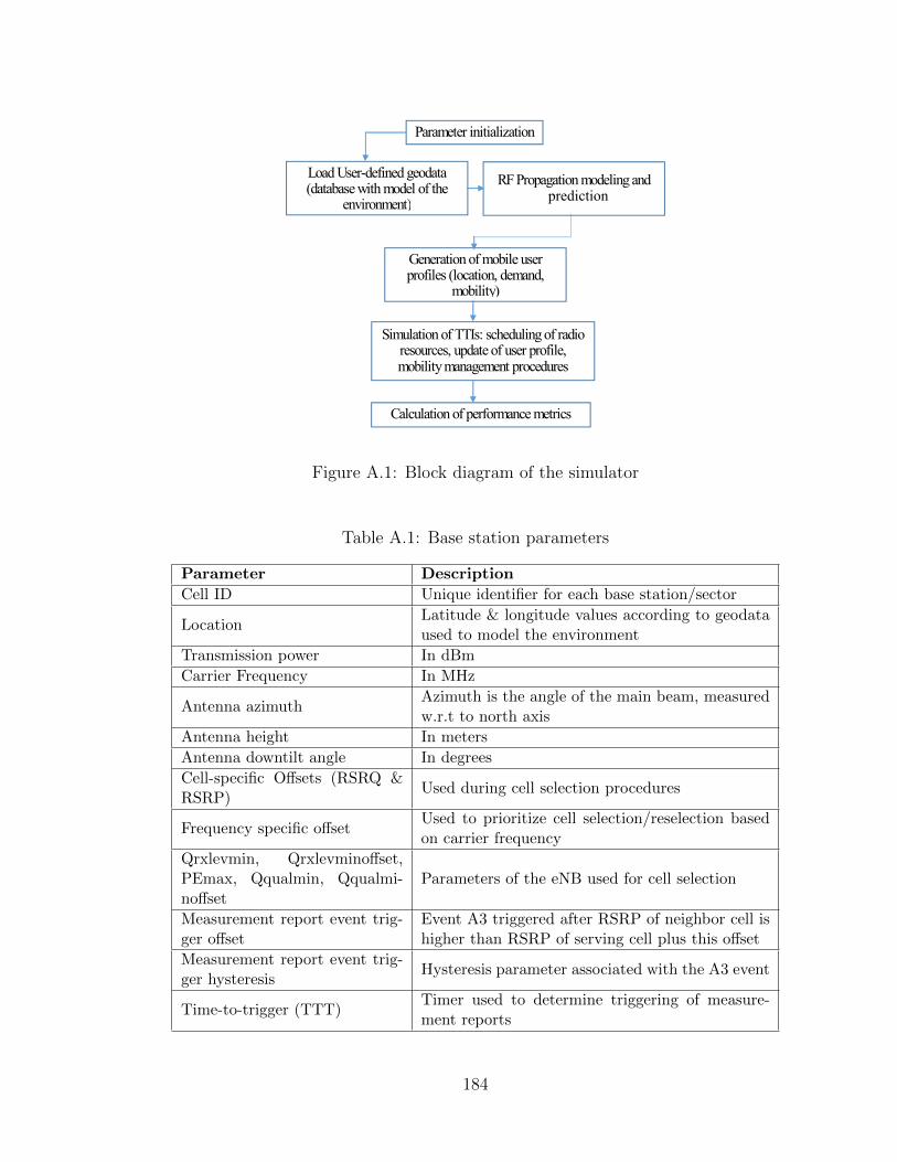
Parameter initialization

Load User-defined geodata(database with model of the

environment)

RF Propagation modeling andprediction

Generation of mobile userprofiles (location, demand,

mobility)

Simulation of TTIs: scheduling of radioresources, update of user profile,mobility management procedures

Calculation of performance metrics

Figure A.1: Block diagram of the simulator

Table A.1: Base station parameters

Parameter Description

Cell ID Unique identifier for each base station/sector

LocationLatitude & longitude values according to geodataused to model the environment

Transmission power In dBm

Carrier Frequency In MHz

Antenna azimuthAzimuth is the angle of the main beam, measuredw.r.t to north axis

Antenna height In meters

Antenna downtilt angle In degrees

Cell-specific Offsets (RSRQ &RSRP)

Used during cell selection procedures

Frequency specific offsetUsed to prioritize cell selection/reselection basedon carrier frequency

Qrxlevmin, Qrxlevminoffset,PEmax, Qqualmin, Qqualmi-noffset

Parameters of the eNB used for cell selection

Measurement report event trig-ger offset

Event A3 triggered after RSRP of neighbor cell ishigher than RSRP of serving cell plus this offset

Measurement report event trig-ger hysteresis

Hysteresis parameter associated with the A3 event

Time-to-trigger (TTT)Timer used to determine triggering of measure-ment reports

184

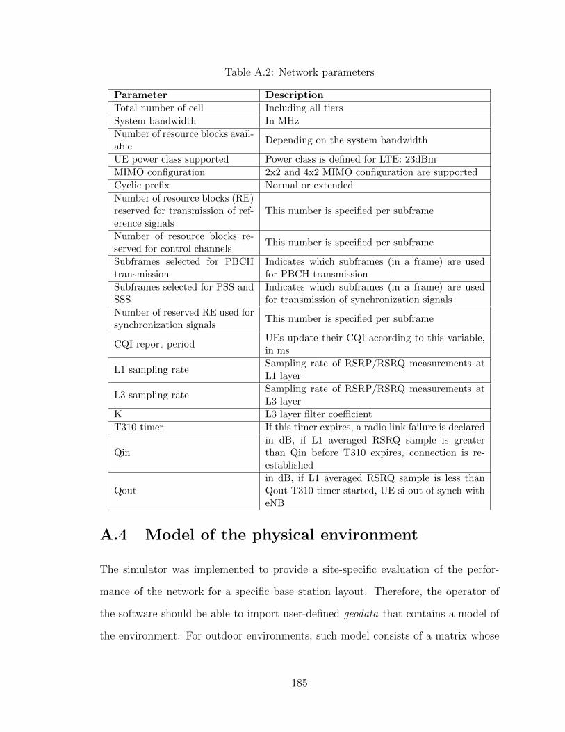
Table A.2: Network parameters

Parameter Description

Total number of cell Including all tiers

System bandwidth In MHz

Number of resource blocks avail-able

Depending on the system bandwidth

UE power class supported Power class is defined for LTE: 23dBm

MIMO configuration 2x2 and 4x2 MIMO configuration are supported

Cyclic prefix Normal or extended

Number of resource blocks (RE)reserved for transmission of ref-erence signals

This number is specified per subframe

Number of resource blocks re-served for control channels

This number is specified per subframe

Subframes selected for PBCHtransmission

Indicates which subframes (in a frame) are usedfor PBCH transmission

Subframes selected for PSS andSSS

Indicates which subframes (in a frame) are usedfor transmission of synchronization signals

Number of reserved RE used forsynchronization signals

This number is specified per subframe

CQI report periodUEs update their CQI according to this variable,in ms

L1 sampling rateSampling rate of RSRP/RSRQ measurements atL1 layer

L3 sampling rateSampling rate of RSRP/RSRQ measurements atL3 layer

K L3 layer filter coefficient

T310 timer If this timer expires, a radio link failure is declared

Qinin dB, if L1 averaged RSRQ sample is greaterthan Qin before T310 expires, connection is re-established

Qoutin dB, if L1 averaged RSRQ sample is less thanQout T310 timer started, UE si out of synch witheNB

A.4 Model of the physical environment

The simulator was implemented to provide a site-specific evaluation of the perfor-

mance of the network for a specific base station layout. Therefore, the operator of

the software should be able to import user-defined geodata that contains a model of

the environment. For outdoor environments, such model consists of a matrix whose

185

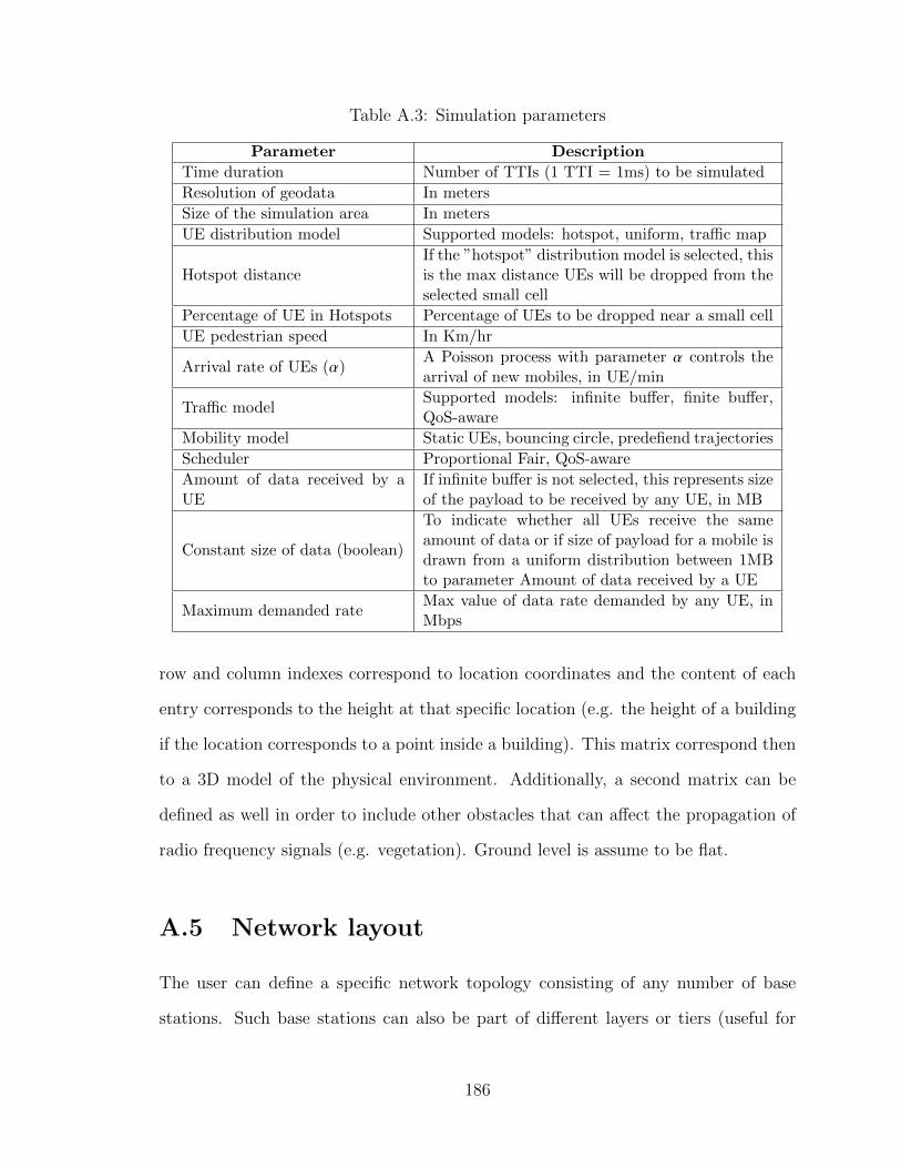
Table A.3: Simulation parameters

Parameter Description

Time duration Number of TTIs (1 TTI = 1ms) to be simulated

Resolution of geodata In meters

Size of the simulation area In meters

UE distribution model Supported models: hotspot, uniform, traffic map

Hotspot distanceIf the ”hotspot” distribution model is selected, thisis the max distance UEs will be dropped from theselected small cell

Percentage of UE in Hotspots Percentage of UEs to be dropped near a small cell

UE pedestrian speed In Km/hr

Arrival rate of UEs (α)A Poisson process with parameter α controls thearrival of new mobiles, in UE/min

Traffic modelSupported models: infinite buffer, finite buffer,QoS-aware

Mobility model Static UEs, bouncing circle, predefiend trajectories

Scheduler Proportional Fair, QoS-aware

Amount of data received by aUE

If infinite buffer is not selected, this represents sizeof the payload to be received by any UE, in MB

Constant size of data (boolean)

To indicate whether all UEs receive the sameamount of data or if size of payload for a mobile isdrawn from a uniform distribution between 1MBto parameter Amount of data received by a UE

Maximum demanded rateMax value of data rate demanded by any UE, inMbps

row and column indexes correspond to location coordinates and the content of each

entry corresponds to the height at that specific location (e.g. the height of a building

if the location corresponds to a point inside a building). This matrix correspond then

to a 3D model of the physical environment. Additionally, a second matrix can be

defined as well in order to include other obstacles that can affect the propagation of

radio frequency signals (e.g. vegetation). Ground level is assume to be flat.

A.5 Network layout

The user can define a specific network topology consisting of any number of base

stations. Such base stations can also be part of different layers or tiers (useful for

186

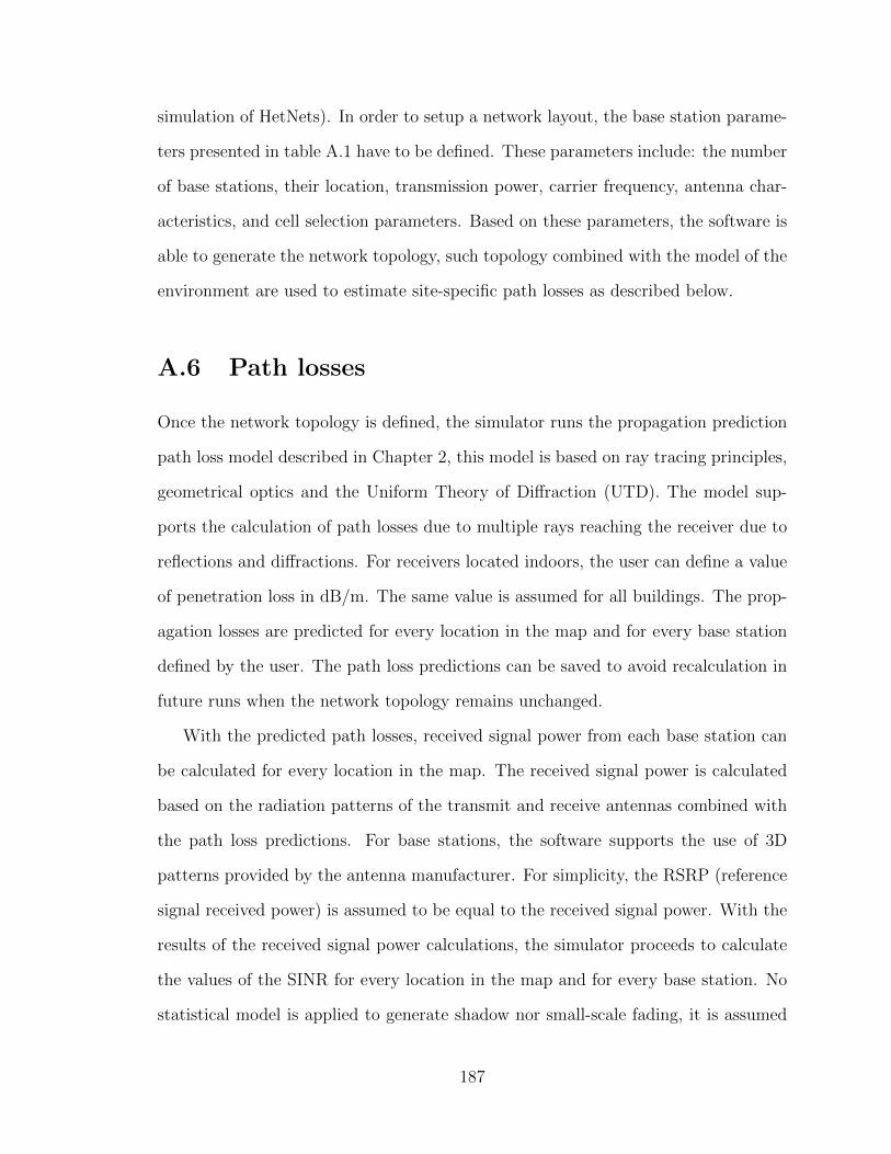
simulation of HetNets). In order to setup a network layout, the base station parame-

ters presented in table A.1 have to be defined. These parameters include: the number

of base stations, their location, transmission power, carrier frequency, antenna char-

acteristics, and cell selection parameters. Based on these parameters, the software is

able to generate the network topology, such topology combined with the model of the

environment are used to estimate site-specific path losses as described below.

A.6 Path losses

Once the network topology is defined, the simulator runs the propagation prediction

path loss model described in Chapter 2, this model is based on ray tracing principles,

geometrical optics and the Uniform Theory of Diffraction (UTD). The model sup-

ports the calculation of path losses due to multiple rays reaching the receiver due to

reflections and diffractions. For receivers located indoors, the user can define a value

of penetration loss in dB/m. The same value is assumed for all buildings. The prop-

agation losses are predicted for every location in the map and for every base station

defined by the user. The path loss predictions can be saved to avoid recalculation in

future runs when the network topology remains unchanged.

With the predicted path losses, received signal power from each base station can

be calculated for every location in the map. The received signal power is calculated

based on the radiation patterns of the transmit and receive antennas combined with

the path loss predictions. For base stations, the software supports the use of 3D

patterns provided by the antenna manufacturer. For simplicity, the RSRP (reference

signal received power) is assumed to be equal to the received signal power. With the

results of the received signal power calculations, the simulator proceeds to calculate

the values of the SINR for every location in the map and for every base station. No

statistical model is applied to generate shadow nor small-scale fading, it is assumed

187

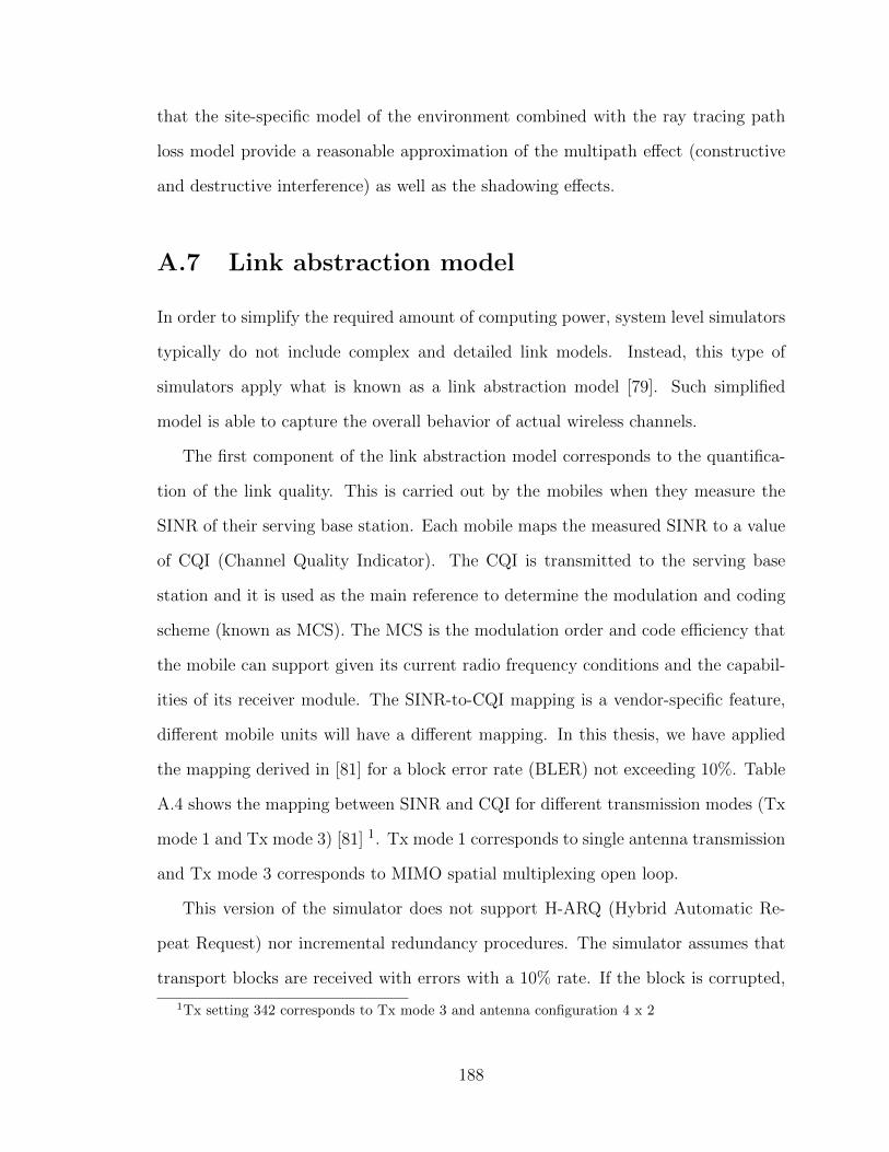
that the site-specific model of the environment combined with the ray tracing path

loss model provide a reasonable approximation of the multipath effect (constructive

and destructive interference) as well as the shadowing effects.

A.7 Link abstraction model

In order to simplify the required amount of computing power, system level simulators

typically do not include complex and detailed link models. Instead, this type of

simulators apply what is known as a link abstraction model [79]. Such simplified

model is able to capture the overall behavior of actual wireless channels.

The first component of the link abstraction model corresponds to the quantifica-

tion of the link quality. This is carried out by the mobiles when they measure the

SINR of their serving base station. Each mobile maps the measured SINR to a value

of CQI (Channel Quality Indicator). The CQI is transmitted to the serving base

station and it is used as the main reference to determine the modulation and coding

scheme (known as MCS). The MCS is the modulation order and code efficiency that

the mobile can support given its current radio frequency conditions and the capabil-

ities of its receiver module. The SINR-to-CQI mapping is a vendor-specific feature,

different mobile units will have a different mapping. In this thesis, we have applied

the mapping derived in [81] for a block error rate (BLER) not exceeding 10%. Table

A.4 shows the mapping between SINR and CQI for different transmission modes (Tx

mode 1 and Tx mode 3) [81] 1. Tx mode 1 corresponds to single antenna transmission

and Tx mode 3 corresponds to MIMO spatial multiplexing open loop.

This version of the simulator does not support H-ARQ (Hybrid Automatic Re-

peat Request) nor incremental redundancy procedures. The simulator assumes that

transport blocks are received with errors with a 10% rate. If the block is corrupted,

1Tx setting 342 corresponds to Tx mode 3 and antenna configuration 4 x 2

188

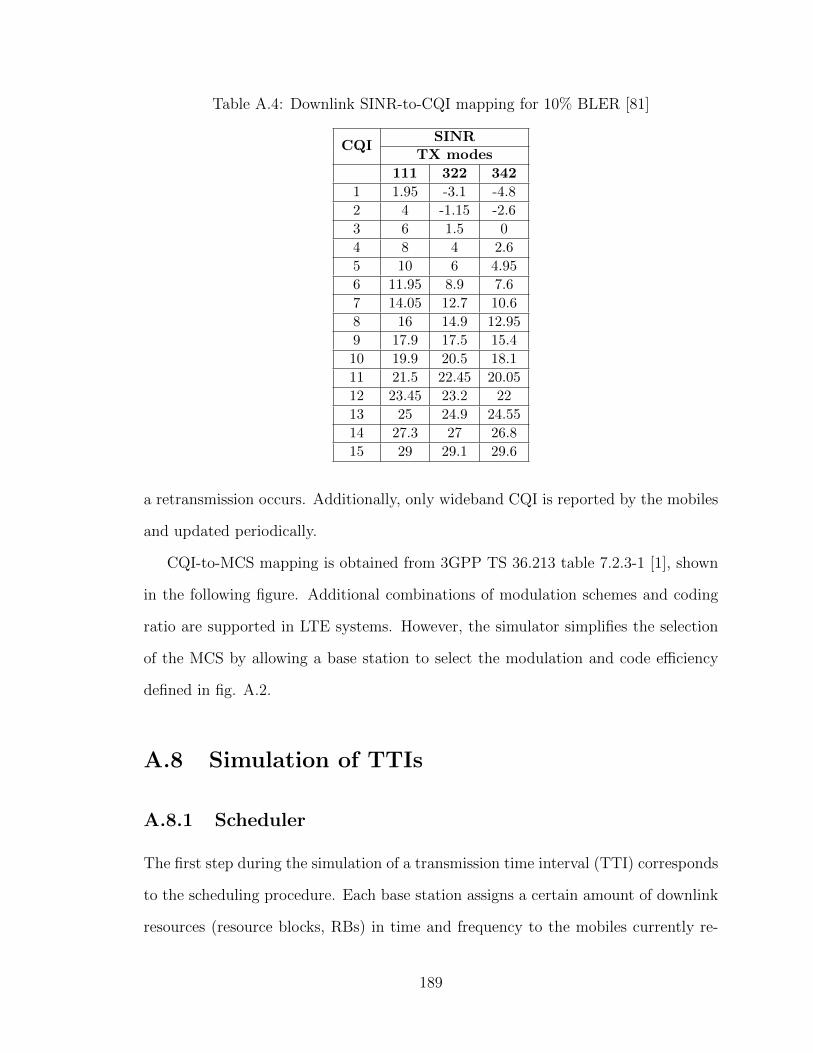
Table A.4: Downlink SINR-to-CQI mapping for 10% BLER [81]

CQISINR

TX modes

111 322 342

1 1.95 -3.1 -4.8

2 4 -1.15 -2.6

3 6 1.5 0

4 8 4 2.6

5 10 6 4.95

6 11.95 8.9 7.6

7 14.05 12.7 10.6

8 16 14.9 12.95

9 17.9 17.5 15.4

10 19.9 20.5 18.1

11 21.5 22.45 20.05

12 23.45 23.2 22

13 25 24.9 24.55

14 27.3 27 26.8

15 29 29.1 29.6

a retransmission occurs. Additionally, only wideband CQI is reported by the mobiles

and updated periodically.

CQI-to-MCS mapping is obtained from 3GPP TS 36.213 table 7.2.3-1 [1], shown

in the following figure. Additional combinations of modulation schemes and coding

ratio are supported in LTE systems. However, the simulator simplifies the selection

of the MCS by allowing a base station to select the modulation and code efficiency

defined in fig. A.2.

A.8 Simulation of TTIs

A.8.1 Scheduler

The first step during the simulation of a transmission time interval (TTI) corresponds

to the scheduling procedure. Each base station assigns a certain amount of downlink

resources (resource blocks, RBs) in time and frequency to the mobiles currently re-

189

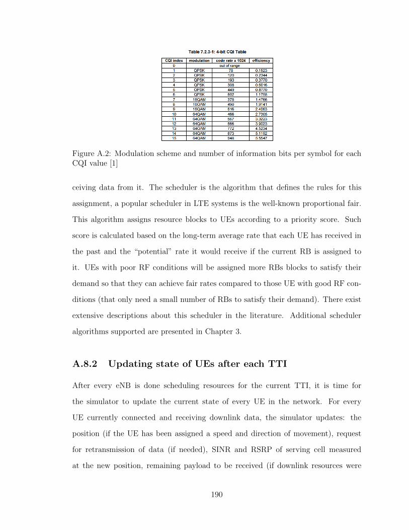
Figure A.2: Modulation scheme and number of information bits per symbol for eachCQI value [1]

ceiving data from it. The scheduler is the algorithm that defines the rules for this

assignment, a popular scheduler in LTE systems is the well-known proportional fair.

This algorithm assigns resource blocks to UEs according to a priority score. Such

score is calculated based on the long-term average rate that each UE has received in

the past and the “potential” rate it would receive if the current RB is assigned to

it. UEs with poor RF conditions will be assigned more RBs blocks to satisfy their

demand so that they can achieve fair rates compared to those UE with good RF con-

ditions (that only need a small number of RBs to satisfy their demand). There exist

extensive descriptions about this scheduler in the literature. Additional scheduler

algorithms supported are presented in Chapter 3.

A.8.2 Updating state of UEs after each TTI

After every eNB is done scheduling resources for the current TTI, it is time for

the simulator to update the current state of every UE in the network. For every

UE currently connected and receiving downlink data, the simulator updates: the

position (if the UE has been assigned a speed and direction of movement), request

for retransmission of data (if needed), SINR and RSRP of serving cell measured

at the new position, remaining payload to be received (if downlink resources were

190

assigned to it), update the CQI value if the CQI-reporting-period has expired, review

of possible triggering of A3 measurement reporting event (for handover operations).

Additionally, the simulator handles the arrival of new UEs based on a Poisson process.

A.9 Throughput calculation

In order to calculate the throughput for a particular UE, the simulator considers the

number of resources blocks allocated to that UE by the scheduler algorithm after a

particular TTI. The number of resource elements (RE) corresponding to the allocated

RBs used for the transmission of information is then determined based on the current

subframe number as well as the frame format selected by the user. Some of the

REs are reserved for the transmission of reference signals, synchronization signals,

broadcast information as well as control signals. Table A.2 shows the parameters

that determine the number of reserved REs. The throughput is then calculated with

(A.1).

T hroughput =# REs used for DL data ∗ info bits per symbol

TTI period(A.1)

Where info bits per symbol are the bits of information per received symbol, this

number is obtained from the table in fig. A.2 according to the reported CQI.

191

Appendix B

Load balancing and adaptiveadjustment of the REB

B.1 Introduction

In this appendix, we investigate the performance of the load balancing algorithm

described in chapter 4 when it is combined with a method to adaptively adjust the

REB of small cells in HetNets. The approach was evaluated under realistic conditions

of an urban environment given a real traffic map. Based on system level simulations,

the overall average data rate gain provided by the load balancing algorithm reached

23% with a significant rate gain for users in the 5th percentile, close to 350%. When

the algorithm was combined with the adaptive adjustment of the REB, an additional

average gain of 50% in the average data rate for low rate users was achieved. With

this bias adjustment method each small cell can adapt its own bias without creating

coverage holes or reaching congestion; as opposed to REB algorithms proposed in

[36–41] that calculate a unique value of the bias for all small cells in the same layer

regardless of their location or local load conditions. The sections in this appendix

have been quoted verbatim from our publication in [57].

B.2 Adaptive bias adjustment

Overloaded base stations can offload more users to neighboring base stations by care-

fully adjusting their cell specific offset or range extension bias (REB). Such offset is

used to encourage (or discourage) users to associate to small cells with low trans-

mission power but lower path losses compared to a distant high power macrocell.

Typically, UEs select the base station that satisfies (B.1) [36]:

j = arg maxj

(RSRPi j + γ j ), ∀ j ∈ J (B.1)

Where γ j is the current value of the REB of the jth eNB, with γ j = 0 for macrocells

and γ j ≥ 0 for small cells.

The higher the value of REB, the larger the coverage area of the small cell. For

an overloaded small cell, it is desirable to reduce the value of the bias such that its

coverage area is reduced and less users will tend to select the small cell during their

cell selection/reselection procedure. On the other hand, if a small cell is underloaded,

then it is desired to expand its coverage area by increasing the value of its bias to

attract more users. The adjustment of the bias should be done carefully in order

to avoid coverage holes (setting a value of the bias too low) or increasing cell edge

interference levels (setting a value of the bias too high).

We propose a simple scheme to adjust the value of the bias for overloaded small

cells based when the the load balancing algorithm described in chapter 4 is applied.

Our approach consists in the evaluation of the values of RSRP reported by users

belonging to the set Tj of each overloaded cell as defined in 4.12. Those values of

RSRP were reported by the UEs that were successfully handed over to underloaded

base stations.

Our approach is based on the following observation: if a user i in Tj is located

in the range extension area of an overloaded eNB j, then it is possible to reduce the

value of the bias, such that other UEs located nearby will be encouraged to select the

underloaded base station to which the user i was handed over.

Consider a user i ∈ Tj that was transferred to a target eNB j∗. User i is located

in the range extension area of the overloaded base station j if the following condition

is satisfied:

193

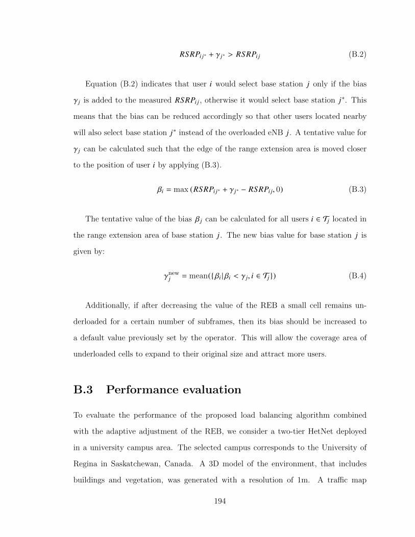
RSRPi j∗ + γ j∗ > RSRPi j (B.2)

Equation (B.2) indicates that user i would select base station j only if the bias

γ j is added to the measured RSRPi j , otherwise it would select base station j∗. This

means that the bias can be reduced accordingly so that other users located nearby

will also select base station j∗ instead of the overloaded eNB j. A tentative value for

γ j can be calculated such that the edge of the range extension area is moved closer

to the position of user i by applying (B.3).

βi = max (RSRPi j∗ + γ j∗ − RSRPi j, 0) (B.3)

The tentative value of the bias β j can be calculated for all users i ∈ Tj located in

the range extension area of base station j. The new bias value for base station j is

given by:

γnewj = mean({βi | βi < γ j, i ∈ Tj }) (B.4)

Additionally, if after decreasing the value of the REB a small cell remains un-

derloaded for a certain number of subframes, then its bias should be increased to

a default value previously set by the operator. This will allow the coverage area of

underloaded cells to expand to their original size and attract more users.

B.3 Performance evaluation

To evaluate the performance of the proposed load balancing algorithm combined

with the adaptive adjustment of the REB, we consider a two-tier HetNet deployed

in a university campus area. The selected campus corresponds to the University of

Regina in Saskatchewan, Canada. A 3D model of the environment, that includes

buildings and vegetation, was generated with a resolution of 1m. A traffic map

194

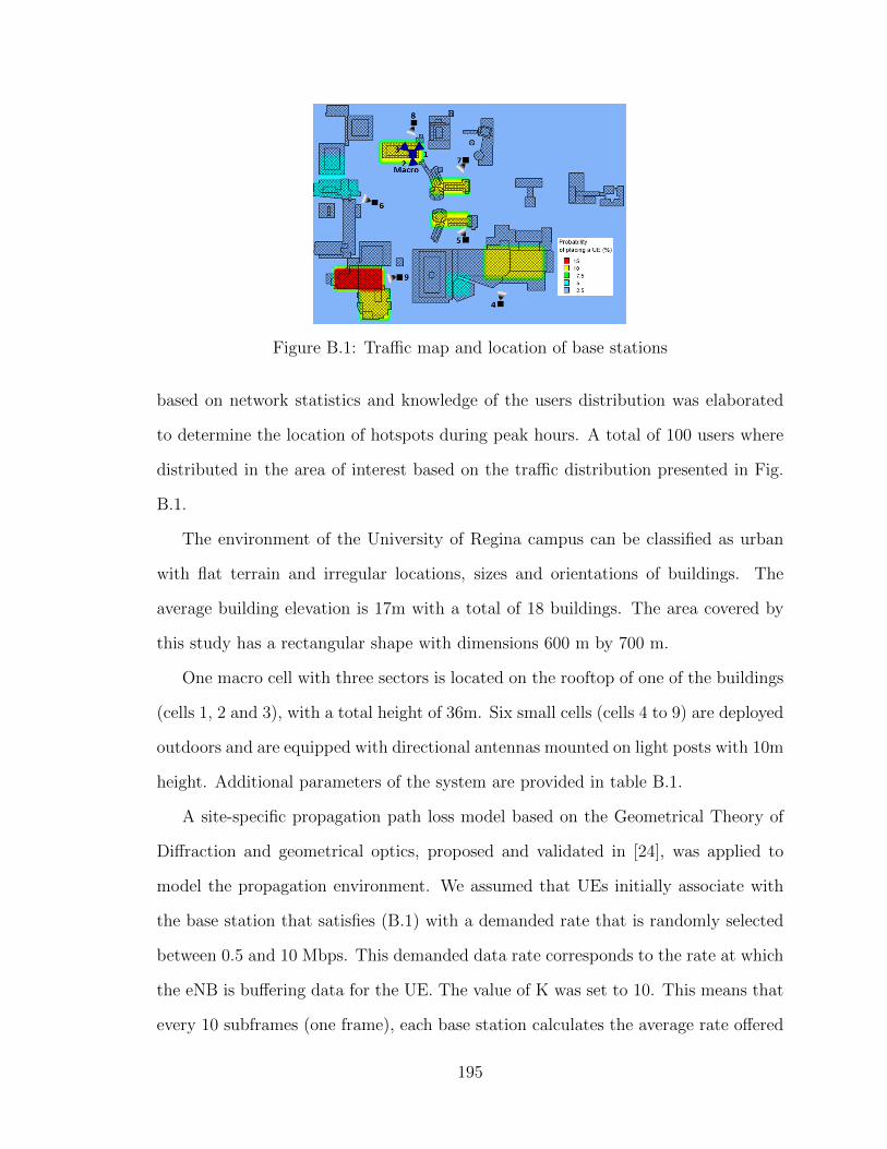
Figure B.1: Traffic map and location of base stations

based on network statistics and knowledge of the users distribution was elaborated

to determine the location of hotspots during peak hours. A total of 100 users where

distributed in the area of interest based on the traffic distribution presented in Fig.

B.1.

The environment of the University of Regina campus can be classified as urban

with flat terrain and irregular locations, sizes and orientations of buildings. The

average building elevation is 17m with a total of 18 buildings. The area covered by

this study has a rectangular shape with dimensions 600 m by 700 m.

One macro cell with three sectors is located on the rooftop of one of the buildings

(cells 1, 2 and 3), with a total height of 36m. Six small cells (cells 4 to 9) are deployed

outdoors and are equipped with directional antennas mounted on light posts with 10m

height. Additional parameters of the system are provided in table B.1.

A site-specific propagation path loss model based on the Geometrical Theory of

Diffraction and geometrical optics, proposed and validated in [24], was applied to

model the propagation environment. We assumed that UEs initially associate with

the base station that satisfies (B.1) with a demanded rate that is randomly selected

between 0.5 and 10 Mbps. This demanded data rate corresponds to the rate at which

the eNB is buffering data for the UE. The value of K was set to 10. This means that

every 10 subframes (one frame), each base station calculates the average rate offered

195

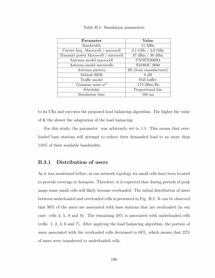
Table B.1: Simulation parameters

Parameter Value

Bandwidth 15 MHz

Carrier freq. Macrocell / microcell 2.1 GHz / 2.6 GHz

Transmit power Macrocell / microcell 47 dBm / 30 dBm

Antenna model macrocell UNNPX306R3

Antenna model microcells S31003U 2600

Antenna pattern 3D (from manufacturer)

Default REB 9 dB

Traffic model Full buffer

Gaussian noise σ2 -174 dBm/Hz

Scheduler Proportional fair

Simulation time 100 ms

to its UEs and executes the proposed load balancing algorithm. The higher the value

of K the slower the adaptation of the load balancing.

For this study, the parameter was arbitrarily set to 1.1. This means that over-

loaded base stations will attempt to reduce their demanded load to no more than

110% of their available bandwidth.

B.3.1 Distribution of users

As it was mentioned before, in our network topology six small cells have been located

to provide coverage to hotspots. Therefore, it is expected that during periods of peak

usage some small cells will likely become overloaded. The initial distribution of users

between underloaded and overloaded cells is presented in Fig. B.2. It can be observed

that 90% of the users are associated with base stations that are overloaded (in our

case: cells 4, 5, 8 and 9). The remaining 10% is associated with underloaded cells

(cells: 1, 2, 3, 6 and 7). After applying the load balancing algorithm, the portion of

users associated with the overloaded cells decreased to 68%, which means that 22%

of users were transferred to underloaded cells.

196

Figure B.2: Distribution of users between overloaded and underloaded eNBs

Table B.2: Fairness indexes of demanded and offered load

Fairness index Without LB With LBDemanded load 0.62 0.9

Offered load 0.52 0.92

B.3.2 Fairness of load balancing

In order to evaluate the performance of the load balancing algorithm, we calculated

the well-known Jain’s fairness index F(L). Where L corresponds to the set of offered

load indexes (or demanded load indexes) of all eNBs. The fairness index has range of

[1/NeN B, 1] , where NeN B is the total number of base stations. A fairness index equal

to unity, indicates that the base stations share the load equally (fair distribution of

the load). The index is calculated according to (B.5).

F (L) =

(∑j∈J L j

)2NeN B ·

∑j∈J

(L j

)2 (B.5)

The fairness index of the offered load and demanded load are shown in table B.2.

When no attempt to balance the load among eNBs is made, the fairness indexes of

the demanded and offered load have poor values of 0.62 and 0.52 respectively. Our

load balancing algorithm was able to distribute the load fairly to achieve values of

fairness indexes around 0.9 and 0.92 for the offered and demanded load respectively.

197

Figure B.3: CDF of the normalized data rate of offloaded cells

B.3.3 Data rate gain evaluation

An important aspect of an effective load balancing algorithm is its capability to

provide gains in the overall network data rate. The overall average data rate for all

users connected to the network was 23% higher when the load was balanced.

In order to quantify the gain in average data rate for cell-edge users (5th percentile),

the cumulative distribution function (CDF) of the normalized average data rate was

calculated. The CDF for the offloaded cells is presented in Fig. B.3. The users

with the lowest 5% normalized rates experienced an improvement of up to 350% in

their average rate, whereas users with already good rates (50th percentile) experienced

an improvement of only 7%. This means that users with low rates received greater

benefit after their base station was offloaded and users that already had good rates

were able to maintain them.

A similar result can be observed from the CDF of the overall normalized rate as

shown in Fig. B.4. Higher gains in rates are provided to users with lower rates. This

is due to the fact that users with low rates are transferred to base stations with spare

capacity, where they are assigned more resources and consequently achieving higher

rates. Once again, users with good rates only experienced marginal gains in their

rate.

The performance of the load balancing algorithm combined with the adaptive

198

Figure B.4: CDF overall normalized data rate for all eNBs

bias adjustment shows an additional average gain of 50% for low data rate users (25th

percentile), compared to the case when only the load balancing algorithm is applied.

B.4 Summary

In this appendix, we described an approach that combines a load balancing algorithm

with an adaptive method to adjust the REB of small cells distributed load balancing

algorithm with adaptive bias adjustment for LTE/LTE-A HetNets. The distributed

algorithm is capable of fairly distributing the load among base stations, requiring a

minimum level of coordination and negligible number of signaling messages between

users and base station. Our simulation results show that a significant gain, around

23%, in the overall average data rate can be achieved. Furthermore, the average data

rate for the low 5% of users is substantially improved with a gain around 350%. The

application of our load balancing algorithm combined with the proposed adaptive

bias adjustment method was able to provide an additional average gain of 50% for

the 25th percentile.

199