1

Marginal Analysis

Basic production (pricing) theory

2

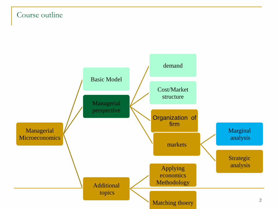
Course outline

Managerial

Microeconomics

Basic Model

Managerial

perspective

demand

Cost/Market

structure

Organization of firm

markets

Marginal

analysis

Strategic

analysis

Additional

topics

Applying

economics

Methodology

Matching thoery

3

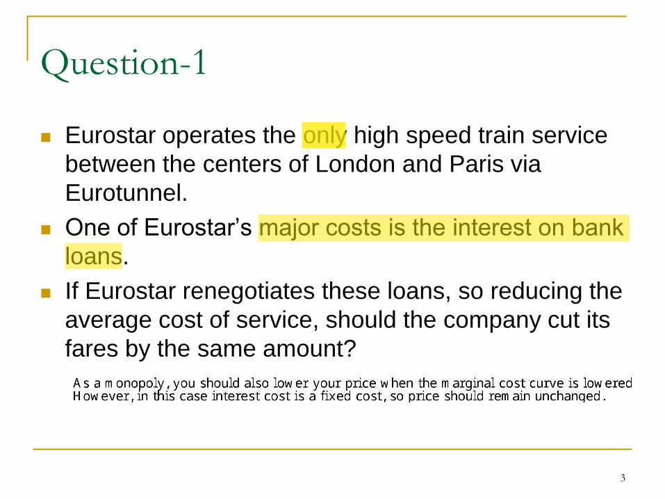
Question-1

Eurostar operates the only high speed train service

between the centers of London and Paris via

Eurotunnel.

One of Eurostar’s major costs is the interest on bank

loans.

If Eurostar renegotiates these loans, so reducing the

average cost of service, should the company cut its

fares by the same amount?

4

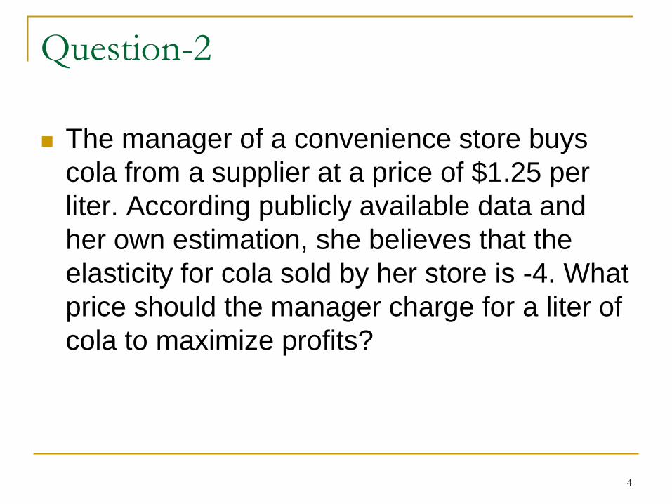
Question-2

The manager of a convenience store buys

cola from a supplier at a price of $1.25 per

liter. According publicly available data and

her own estimation, she believes that the

elasticity for cola sold by her store is -4. What

price should the manager charge for a liter of

cola to maximize profits?

5

Lecture Outline

1. Managing without market power Optimal production rate

Profitability

2. Managing with market power Optimal production rate (or pricing) (three views)

Multiplant output decision

Optimal advertising rule

3. Measuring market power

6

1. Managing without market power

No market power: your firm’s participation has no impact on the market.

price taker: at the market price, your firm faces a horizontal demand curve within your production capacity.

Given a price, what is your optimal strategy?

7

1. Managing without market power

Profitability

The future is not very bright: make ____ economic

profit! (why?)

But it’s not extremely dark either: _____ economic

profit ≠ ______ accounting profit

8

2. Managing with market power

Market power

Your firm Faces a downward-sloping demand curve

You may choose either the price or the quantity (but not both!)

Optimal production (pricing) strategy (view 1)

Set price (quantity) such that

______________=____________

9

2.1.1 Marginal Revenue

Marginal Revenue: the change in total

revenue arising from selling an additional

unit.

To sell an additional unit, a monopolist must

reduce its price.

Inframarginal Units: are those other than the

marginal unit.

Marginal Revenue = Price - Loss of revenue on

the inframarginal units

10

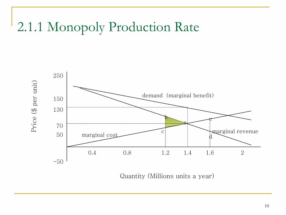
2.1.1 Monopoly Production Rate

-50

50

70

130

150

250

0.4 0.8 1.2 1.4 1.6 2

demand (marginal benefit)

marginal revenue marginal cost

c

a b e

d

Quantity (Millions units a year)

11

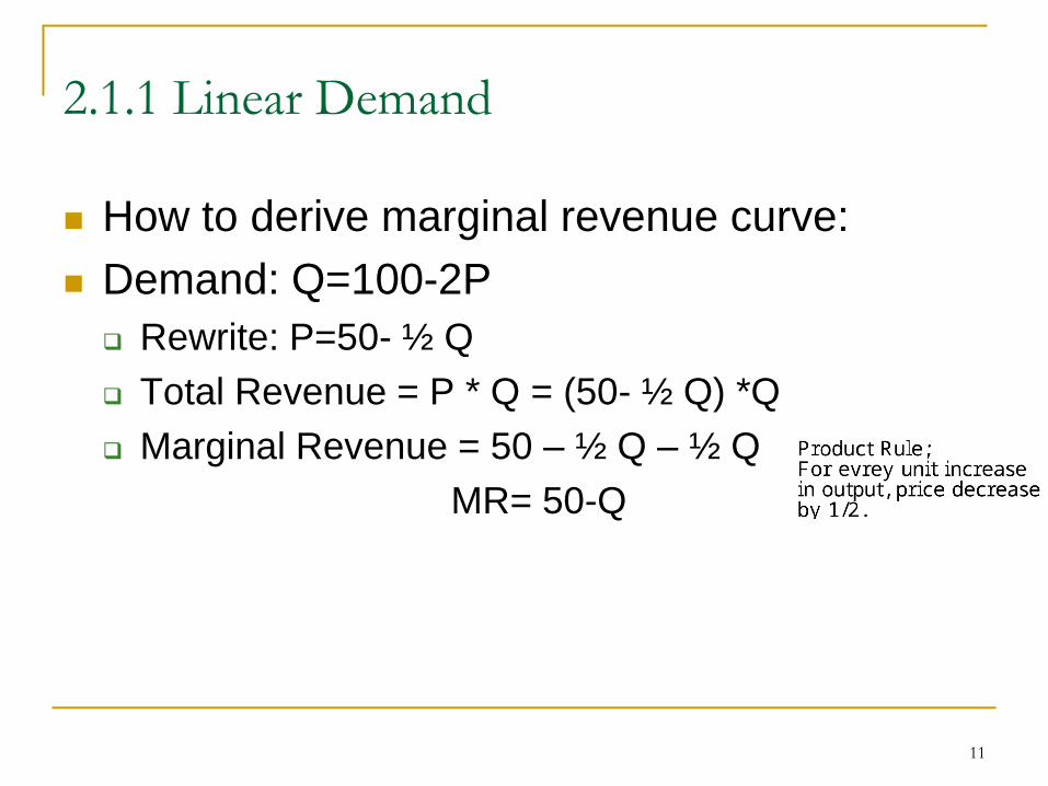
2.1.1 Linear Demand

How to derive marginal revenue curve:

Demand: Q=100-2P

Rewrite: P=50- ½ Q

Total Revenue = P * Q = (50- ½ Q) *Q

Marginal Revenue = 50 – ½ Q – ½ Q

MR= 50-Q

12

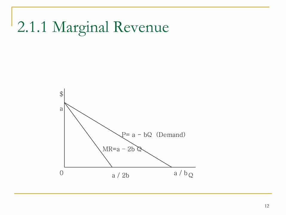
2.1.1 Marginal Revenue

$

Q

P= a - bQ (Demand)

MR=a – 2b Q

a

0 a / 2b a / b

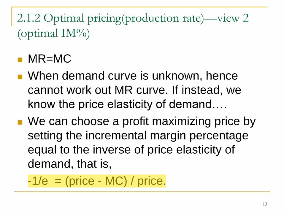
2.1.2 Optimal pricing(production rate)—view 2

(optimal IM%)

MR=MC

When demand curve is unknown, hence

cannot work out MR curve. If instead, we

know the price elasticity of demand….

We can choose a profit maximizing price by

setting the incremental margin percentage

equal to the inverse of price elasticity of

demand, that is,

-1/e = (price - MC) / price.

13

14

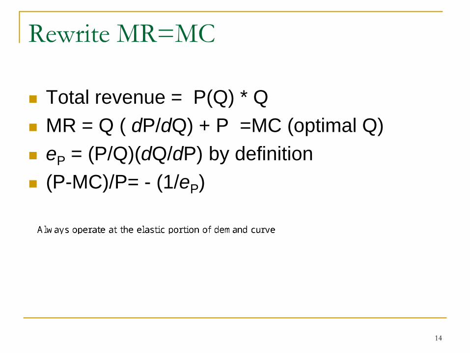
Rewrite MR=MC

Total revenue = P(Q) * Q

MR = Q ( dP/dQ) + P =MC (optimal Q)

eP = (P/Q)(dQ/dP) by definition

(P-MC)/P= - (1/eP)

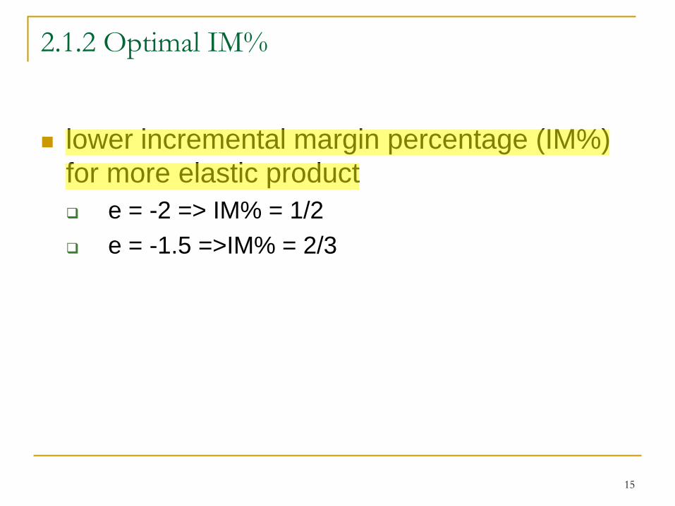
2.1.2 Optimal IM%

lower incremental margin percentage (IM%)

for more elastic product

e = -2 => IM% = 1/2

e = -1.5 =>IM% = 2/3

15

16

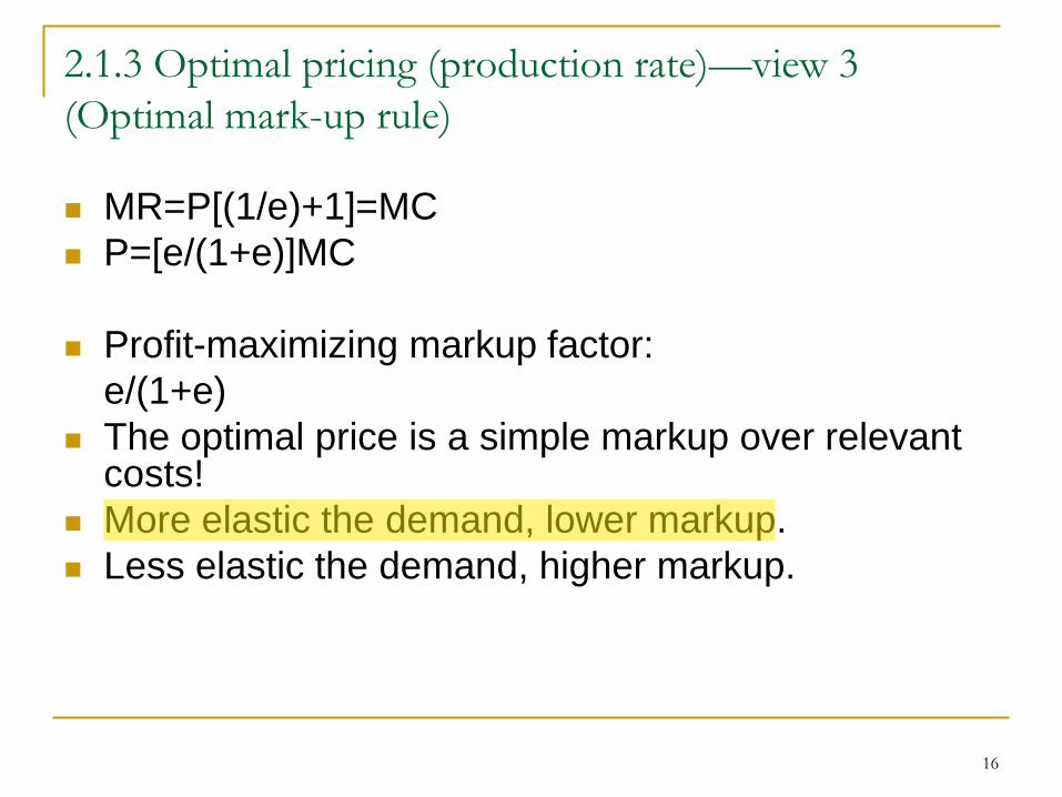
2.1.3 Optimal pricing (production rate)—view 3

(Optimal mark-up rule)

MR=P[(1/e)+1]=MC

P=[e/(1+e)]MC

Profit-maximizing markup factor:

e/(1+e)

The optimal price is a simple markup over relevant costs!

More elastic the demand, lower markup.

Less elastic the demand, higher markup.

17

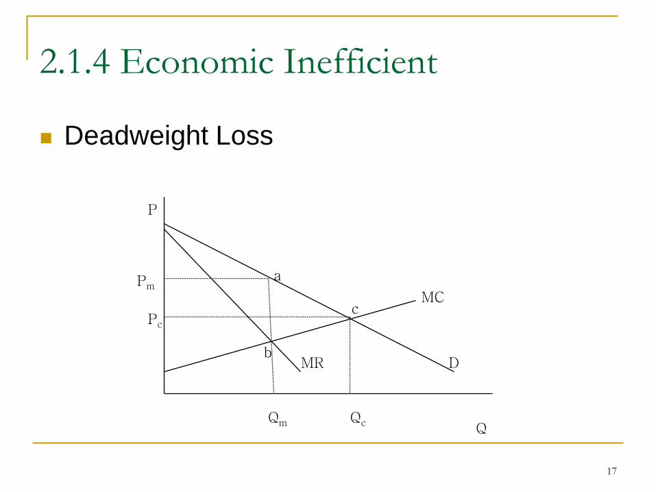
2.1.4 Economic Inefficient

Deadweight Loss

P

Q

MC

D MR

Qc Qm

Pc

Pm a

b

c

18

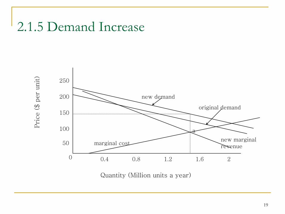
2.1.5 Demand Change

Find new quantity where marginal revenue = marginal cost

• demand shift

should change price

• new quantity and price depend on both new demand and costs

19

2.1.5 Demand Increase

0

50

100

150

200

250

0.4 0.8 1.2 1.6 2

marginal cost

new demand

original demand

new marginal revenue

a

Quantity (Million units a year)

Pri

ce (

$ p

er

unit)

20

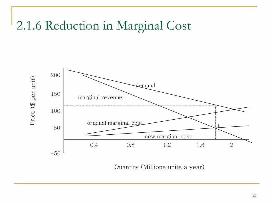
2.1.6 Cost Change

Find new quantity where marginal revenue =

marginal cost

• change in fixed cost

should not change price

• change in marginal cost

should change price (but not equal to

change in MC)

21

2.1.6 Reduction in Marginal Cost

-50

50

100

150

200

0.4 0.8 1.2 1.6 2

demand

Quantity (Millions units a year)

k

marginal revenue

original marginal cost

new marginal cost

22

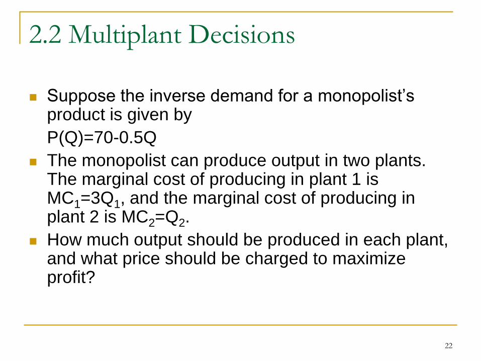
2.2 Multiplant Decisions

Suppose the inverse demand for a monopolist’s product is given by

P(Q)=70-0.5Q

The monopolist can produce output in two plants. The marginal cost of producing in plant 1 is MC1=3Q1, and the marginal cost of producing in plant 2 is MC2=Q2.

How much output should be produced in each plant, and what price should be charged to maximize profit?

23

2.2 Multiplant Decisions

Multiplant Output Rule

MR(Q)=MC1(Q1)=MC2(Q2).

24

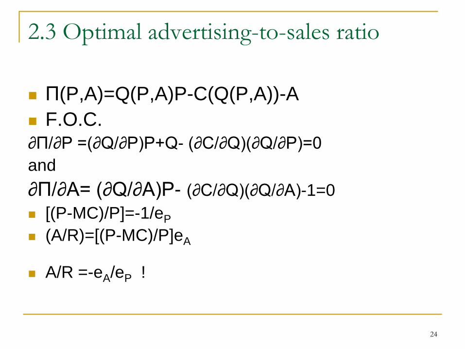
2.3 Optimal advertising-to-sales ratio

Π(P,A)=Q(P,A)P-C(Q(P,A))-A

F.O.C.

∂Π/∂P =(∂Q/∂P)P+Q- (∂C/∂Q)(∂Q/∂P)=0

and

∂Π/∂A= (∂Q/∂A)P- (∂C/∂Q)(∂Q/∂A)-1=0

[(P-MC)/P]=-1/eP

(A/R)=[(P-MC)/P]eA

A/R =-eA/eP !

25

2.3 Optimal advertising-to-sales ratio

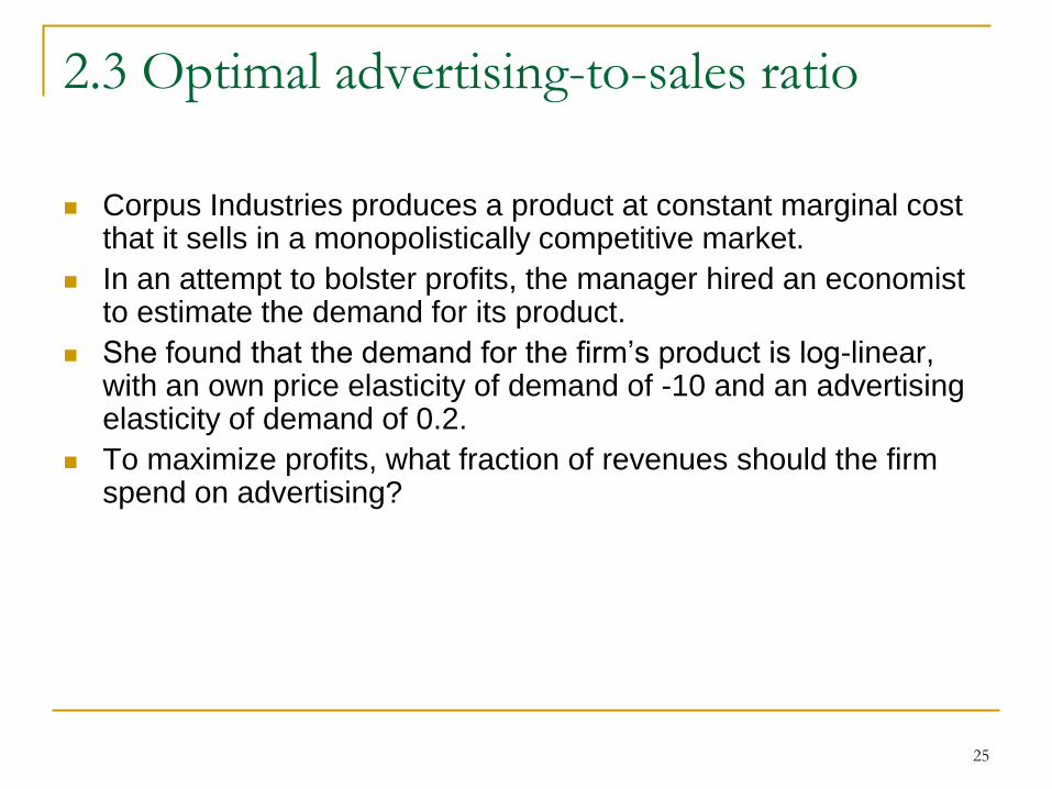
Corpus Industries produces a product at constant marginal cost that it sells in a monopolistically competitive market.

In an attempt to bolster profits, the manager hired an economist to estimate the demand for its product.

She found that the demand for the firm’s product is log-linear, with an own price elasticity of demand of -10 and an advertising elasticity of demand of 0.2.

To maximize profits, what fraction of revenues should the firm spend on advertising?

26

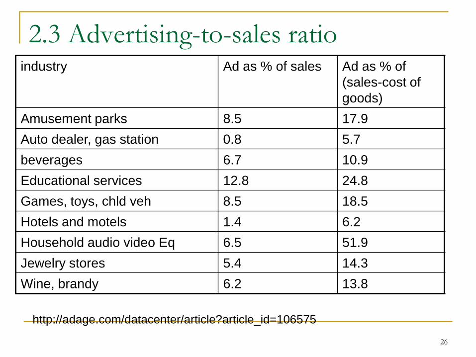
2.3 Advertising-to-sales ratio industry Ad as % of sales Ad as % of

(sales-cost of

goods)

Amusement parks 8.5 17.9

Auto dealer, gas station 0.8 5.7

beverages 6.7 10.9

Educational services 12.8 24.8

Games, toys, chld veh 8.5 18.5

Hotels and motels 1.4 6.2

Household audio video Eq 6.5 51.9

Jewelry stores 5.4 14.3

Wine, brandy 6.2 13.8

http://adage.com/datacenter/article?article_id=106575

27

3. Potential Competition

Competition will push down the market price toward

the long-run average cost.

Sometimes, potential competition is sufficient to

keep the market price close to the long-run average

cost.

28

3. Measure monopoly (market) power

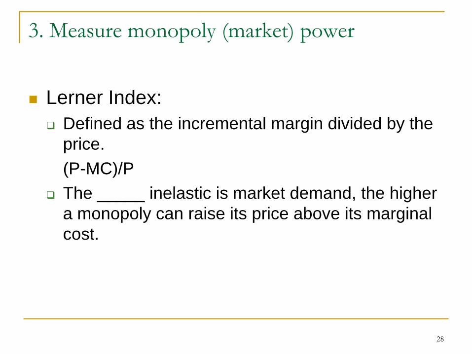
Lerner Index:

Defined as the incremental margin divided by the

price.

(P-MC)/P

The _____ inelastic is market demand, the higher

a monopoly can raise its price above its marginal

cost.

29

3. Lerner Index

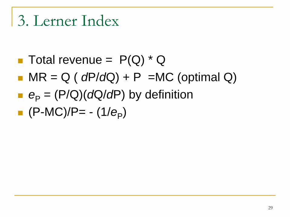
Total revenue = P(Q) * Q

MR = Q ( dP/dQ) + P =MC (optimal Q)

eP = (P/Q)(dQ/dP) by definition

(P-MC)/P= - (1/eP)

30

3. Lerner Index

Lerner Index is a ______, hence we can

compare different markets .

It captures the impact of ________

competition.

31

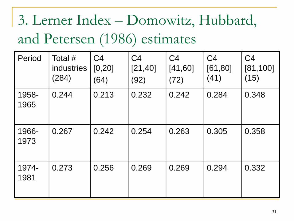
3. Lerner Index – Domowitz, Hubbard,

and Petersen (1986) estimates Period Total #

industries

(284)

C4

[0,20]

(64)

C4

[21,40]

(92)

C4

[41,60]

(72)

C4

[61,80]

(41)

C4

[81,100]

(15)

1958-

1965

0.244

0.213 0.232 0.242 0.284 0.348

1966-

1973

0.267 0.242 0.254 0.263 0.305 0.358

1974-

1981

0.273 0.256 0.269 0.269 0.294 0.332

32

Common Misconception

Monopoly’s supply curve?

Duopoly’s supply curve?

33

Topic Intended Learning Outcomes

Students should be able to: 6.1 Explain and calculate the profit maximizing/ revenue maximizing

production rate under perfect competition, monopolistic

competition, and monopoly.

6.2 Explain and apply multi-plant decision rule.

6.3 Explain and apply optimal advertising rules.

6.4 Calculate Lerner index and explain why it is a good measure of

market power.

6.5 Calculate Deadweight loss of monopoly.