Embed Size (px)
Citation preview
Changes in the predictability of the North
Atlantic ocean under global warming
Dissertation zur Erlangung des Doktorgrades
an der Fakultat fur Mathematik, Informatik und
Naturwissenschaften
Fachbereich Geowissenschaften
der Universitat Hamburg
vorgelegt von
Matthias Fischer
Hamburg, 2015

Tag der Disputation: 18.12.2015
Folgende Gutachter empfehlen die Annahme der Dissertation:
Prof. Dr. Johanna Baehr
Dr. Wolfgang A. Muller


i
Abstract
The North Atlantic Ocean plays an important role for the European and the NorthAmerican climate. Hence, predictions of the North Atlantic climate on seasonal-to-decadal time scales are of growing interest. The North Atlantic Ocean is projectedto change with global warming. Projections show an increase of surface tempera-tures and a reduction in the Atlantic meridional overturning circulation (AMOC)and the Atlantic meridional ocean heat transport (OHT). Yet, whether globalwarming a↵ects the seasonal cycle and the decadal predictability of the AMOCand the OHT is still unknown. In this thesis I investigate changes in the AMOCand OHT seasonal cycle under global warming. In a second step, I focus on changesin potential predictability of the AMOC and the OHT that might result from po-tential changes in the seasonal cycle from the present climate state to a futureclimate state.First, I investigate the e↵ect of a projected reduction in the AMOC and in theOHT on their seasonal cycles. I analyze climate projection experiments performedwith the Max-Planck Institute Earth System Model (MPI-ESM) for the CoupledModel Intercomparison Project phase 5 (CMIP5). My results suggest shifts in theAMOC and OHT seasonal cycles that predominantly result from changes in thewind-driven circulation. Analyzing long-term implications in the RCP8.5 (repre-sentative concentration pathway) scenario until the end of the 23rd century, I finda northward shift of 5 degrees and latitude dependent temporal shifts of 1 to 6months in the seasonal cycle. Similar, but less intense changes are found until themiddle of the 21st century in RCP4.5 and RCP8.5, in particular in the subtropicalgyre (STG) around 25�N and in the subpolar gyre (SPG) around 50�N.Second, I analyze changes in the potential predictability of the AMOC and OHT oninter-annual to decadal time scales under global warming. In MPI-ESM, I generatetwo hindcast ensembles for (i) the current climate state in the CMIP5 historicalsimulation starting in 1995 and extended with RCP4.5 after 2005 (HISTens) and(ii) a future climate state in RCP4.5 starting in 2045 (RCPens). Changes in thepotential predictability are assessed by means of the anomaly correlation coe�-cient (ACC), the reliability and the Brier Skill Score (BSS) of the hindcasts formultiyear means and multiyear seasonal means.The potential predictability of the AMOC and the OHT changes predominantlyat latitudes where considerable changes are found in the seasonal cycle. For theAMOC in HISTens, the STG reveals longer predictable lead times compared to theSPG resulting predominately from the predictability of the geostrophic transportand the predictability of multiyear summer means. The ACC of the AMOC isreduced from HISTens to RCPens in the STG and the SPG, as is the reliability. InRCPens, the reduction in the predictability of the AMOC results predominatelyfrom a reduced predictability of summer means.For the OHT in HISTens, the SPG reveals longer predictable lead times comparedto the STG. Between HISTens and RCPens, the ACC is reduced in the STG andincreased in the SPG with longer predictable lead times in the SPG compared toHISTens. The reliability and the BSS are reduced in the STG and SPG betweenHISTens and RCPens, even though winter and summer show reliable predictionsin the SPG. The reduction in the predictability of the OHT results from changesin all seasons.The results of this thesis further highlight that changes in the seasonal cycle, inconnection with an overall decrease in the variance of yearly means, lead to a re-duction in the potential predictability under global warming, while an increasedvariance leads to an increased potential predictability.

iii
Zusammenfassung
Der Nordatlantische Ozean ist fur das Klima in Europa und Nordamerikavon großer Bedeutung. Daher sind Vorhersagen des nordatlantischenKlimas auf saisonalen bis dekadischen Zeitskalen von besonderem Interesse.Klimaprojektionen zeigen Veranderungen des Nordatlantiks im Zuge der globalenErwarmung. Diese beinhalten einen Anstieg der Oberflachentemperaturen,eine Abnahme der Atlantischen meridionalen Umwaltzzirkulation (AMOC)sowie eine Abnahme des meridionalen ozeanischen Warmetransportes (OHT).Bisher ist nicht untersucht, ob die globale Erwarmung den Jahresgang und diedekadische Vorhersagbarkeit der AMOC und des OHT beeinflusst. In dieserArbeit untersuche ich Veranderungen im Jahresgang der AMOC und des OHTunter Einfluss des Klimawandels. In einem weiteren Schritt untersuche ichVeranderungen der potentiellen Vorhersagbarkeit der AMOC und des OHT. Diesekonnen aus potentiellen Veranderungen des Jahresgangs von dem derzeitigenKlimazustand zu einem zukunftigen Klimazustand resultieren.In einem ersten Schritt analysiere ich Jahresgangsanderungen der AMOC unddes OHT unter Einfluss des Klimawandels. Dazu werden Klimaprojektionenherangezogen, die im gekoppelten Max-Planck-Erdsystemmodell (MPI-ESM)im Rahmen des Coupled Model Intercomparisson Project phase 5 (CMIP5)durchgefuhrt wurden. Meine Ergebnisse zeigen Verschiebungen im Jahresgang derAMOC und des OHT, die in erster Linie aus Anderungen der windgetriebenenZirkulation resultieren. Anderungen bis Ende des 23. Jahrhunderts imKlimaanderungsszenario RCP8.5 (RCP=representative concentration pathway)zeigen eine Nordwartsverschiebung um 5� und breitenabhangige zeitlicheVerschiebungen von 1 bis 6 Monaten im Jahresgang sowie Anderungen in derJahreszeitenamplitude. Ahnliche, wenn auch schwachere Anderungen, treten biszur Mitte des 21. Jahrhunderts in RCP4.5 und RCP8.5 auf. Diese zeigen sichbesonders im Subtropenwirbel (STG) um 25�N und im Subpolarwirbel (SPG) um50�N.Anschließend werden Veranderungen der potentiellen Vorhersagbarkeitder AMOC und des OHT unter Einfluss der globalen Erwarmung aufinterannualen bis dekadischen Zeitskalen untersucht. Dazu werden zweiEnsemble-Vorhersage-Experimente (Hindcasts) in MPI-ESM erstellt: zumeinen fur den derzeitigen Klimazustand im CMIP5 historischen Lauf, dermit dem RCP4.5 Szenario erweitert wird (HISTens), und zum anderen fureinen zukunftigen Klimazustand in RCP4.5 (RCPens). Veranderungen derVorhersagbarkeit werden mit Hilfe des Anomaliekorrelationskoe�zienten (ACC),der reliability und des Brier Skill Scores (BSS) der Hindcasts fur Jahresmittelund saisonale Mittel untersucht.Die potentielle Vorhersagbarkeit der AMOC und des OHT andert sich besondersan Breitengraden mit großen Anderungen im Jahresgang. Die AMOC zeigt inHISTens eine langere Vorhersagbarkeitszeit (predictable lead times) im STGals im SPG. Dies ist bedingt durch die Vorhersagbarkeit des geostrophischenTransportes und der Vorhersagbarkeit von Sommermitteln. Vom derzeitigenZustand in HISTens zu RCPens verringert sich der ACC – und gleichzeitig diereliability – der AMOC im STG und SPG. Die verringerte Vorhersagbarkeit inRCPens resultiert hauptsachlich aus der verringerten Vorhersagbarkeit derSommermittelwerte.

iv
Im OHT zeigt der SPG fur den derzeitigen Klimazustand in HISTens langereVorhersagbarkeit im Vergleich zum STG. Von HISTens hinzu RCPens ist der ACCim STG verringert und im SPG erhoht. Der OHT zeigt langere Vorhersagezeitenim SPG im Vergleich zu HISTens. Die reliability und der BSS sind im STGund SPG verringert von HISTens zu RCPens. Sommer- und Wintermittelzeigen jedoch eine gewisse reliability der Vorhersagen im SPG. Die generelleVerringerung der Vorhersagbarkeit des OHT resultiert aus Anderungen in allenJahreszeiten.Die Ergebnisse dieser Arbeit heben außerdem hervor, dass Anderungenim Jahresgang, zusammen mit einer generellen Verringerung der Varianzvon Jahresmitteln, die potentielle Vorhersagbarkeit unter Einfluss derglobalen Erwarmung verringern, wobei eine verstarkte Varianz die potentielleVorhersagbarkeit erhoht.
Contents
Abstract . . . . . . . . . . . . . . . . . . . . . . . . . . . . . . . . i
Zusammenfassung . . . . . . . . . . . . . . . . . . . . . . . . . . iii
1 Introduction 1
1.1 Motivation . . . . . . . . . . . . . . . . . . . . . . . . . . . . . 1
1.1.1 Global warming and the North Atlantic ocean circulation 1
1.1.2 Decadal predictability . . . . . . . . . . . . . . . . . . 5
1.2 Objectives of the thesis . . . . . . . . . . . . . . . . . . . . . . 8
1.3 Outline of the thesis . . . . . . . . . . . . . . . . . . . . . . . 9
2 Long-term changes in the Atlantic meridional heat transport
and its seasonal cycle 11
2.1 The Atlantic meridional heat transport seasonal cycle in a
MPI-ESM climate projection . . . . . . . . . . . . . . . . . . . 11
2.1.1 Introduction . . . . . . . . . . . . . . . . . . . . . . . . 12
2.1.2 Model and Methods . . . . . . . . . . . . . . . . . . . 17
vi Contents
2.1.3 Mean changes in the Atlantic meridional overturning
circulation and meridional heat transport . . . . . . . . 25
2.1.4 Changes in the seasonal cycle of the Atlantic meridional
heat transport . . . . . . . . . . . . . . . . . . . . . . . 28
2.1.5 Discussion . . . . . . . . . . . . . . . . . . . . . . . . . 38
2.1.6 Conclusions . . . . . . . . . . . . . . . . . . . . . . . . 41
2.2 The seasonal cycle of the Atlantic meridional heat transport
in potential temperature coordinates . . . . . . . . . . . . . . 45
2.2.1 Introduction . . . . . . . . . . . . . . . . . . . . . . . . 45
2.2.2 The heat function as a representation of the meridional
heat transport . . . . . . . . . . . . . . . . . . . . . . . 46
2.2.3 The AMOC, the heat function and the associated
meridional heat transport seasonal cycle in MPI-ESM . 48
2.2.4 Summary and Conclusions . . . . . . . . . . . . . . . . 55
3 Near-term changes in the seasonal cycle of the Atlantic
meridional heat transport and the Atlantic meridional
overturning circulation 59
3.1 Introduction . . . . . . . . . . . . . . . . . . . . . . . . . . . . 59
3.2 Methods . . . . . . . . . . . . . . . . . . . . . . . . . . . . . . 60
3.3 Changes in the seasonal cycle of the AMOC and the OHT until
the middle of the 21st century . . . . . . . . . . . . . . . . . . 61
3.3.1 Seasonal peak-to-peak amplitude . . . . . . . . . . . . 64
3.3.2 Temporal shift in the seasonal minima and maxima . . 67
Contents vii
3.4 Summary . . . . . . . . . . . . . . . . . . . . . . . . . . . . . 70
3.5 Conclusions . . . . . . . . . . . . . . . . . . . . . . . . . . . . 71
4 Potential predictability of the North Atlantic ocean circula-
tion in the present and future climate 73
4.1 Introduction . . . . . . . . . . . . . . . . . . . . . . . . . . . . 73
4.2 Methods . . . . . . . . . . . . . . . . . . . . . . . . . . . . . . 77
4.2.1 Model and ensemble generation . . . . . . . . . . . . . 77
4.2.2 Predictability analysis . . . . . . . . . . . . . . . . . . 79
4.3 Predictability of the AMOC . . . . . . . . . . . . . . . . . . . 84
4.3.1 Yearly mean AMOC . . . . . . . . . . . . . . . . . . . 84
4.3.2 Multiyear seasonal means . . . . . . . . . . . . . . . . 87
4.3.3 Yearly mean geostrophic transport . . . . . . . . . . . 91
4.3.4 Multiyear seasonal means of the geostrophic transport 93
4.4 Predictability of the OHT . . . . . . . . . . . . . . . . . . . . 95
4.4.1 Yearly means of the OHT . . . . . . . . . . . . . . . . 95
4.4.2 Multiyear seasonal means of the OHT . . . . . . . . . 97
4.4.3 Yearly means of the overturning and gyre heat transport101
4.4.4 Contribution of the overturning and gyre heat trans-
port to the predictability of the OHT . . . . . . . . . . 103
4.4.5 Multiyear seasonal means of the overturning and gyre
heat transport . . . . . . . . . . . . . . . . . . . . . . . 105

viii Contents
4.5 Summary and Discussion . . . . . . . . . . . . . . . . . . . . . 111
4.6 Conclusions . . . . . . . . . . . . . . . . . . . . . . . . . . . . 116
5 Summary and Conclusions 119
6 Bibliography 129
1 Introduction
1.1 Motivation
1.1.1 Global warming and the North Atlantic ocean
circulation
The North Atlantic Ocean has received increased attention in recent years
due to its key role for the regional and the global climate. The North At-
lantic Ocean is shown to impact local climate phenomena such as Atlantic
hurricanes or Sahel drought (e.g., Knight et al., 2006, Zhang and Delworth,
2006), the North American and European climate (e.g., Sutton and Hodson,
2005, Pohlmann et al., 2006, Sutton and Dong, 2012) or climate phenom-
ena with global impacts, such as the North Atlantic Oscillation (NAO; e.g.,
Czaja et al., 1999, Czaja and Frankignoul, 2002, Frankignoul et al., 2013,
Gastineau and Frankignoul, 2015). Climate model simulations suggest that
fluctuations in the Atlantic meridional overturning circulation (AMOC) are
linked to decadal climate variability in the North Atlantic sector (e.g. Latif
and Keenlyside, 2011, Siedler et al., 2013) with important socio-economic
impacts (e.g. Srokosz et al., 2012, Smeed et al., 2013).
Via the Atlantic Multidecadal Oscillation (AMO), a number of these climate
phenomena has been linked to the variability of North Atlantic sea surface
temperatures (SST; e.g., Delworth and Greatbatch, 2000, Knight et al., 2005,
Msadek and Frankignoul, 2009, Zhang and Wang, 2013). In particular the
AMOC and the associated Atlantic meridional ocean heat transport (OHT)
2 1.1. Motivation
a b c
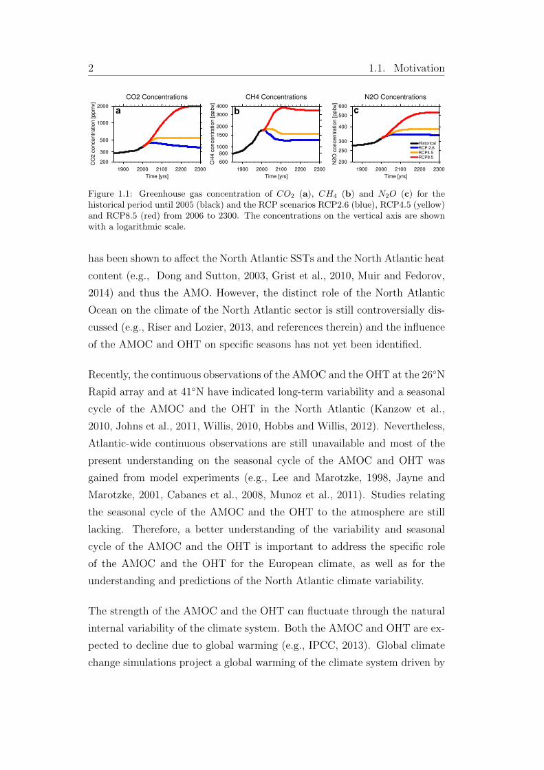
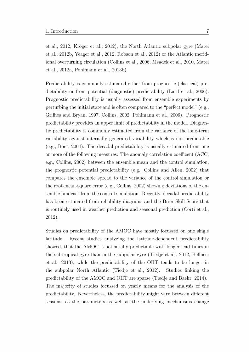
Figure 1.1: Greenhouse gas concentration of CO2 (a), CH4 (b) and N2O (c) for thehistorical period until 2005 (black) and the RCP scenarios RCP2.6 (blue), RCP4.5 (yellow)and RCP8.5 (red) from 2006 to 2300. The concentrations on the vertical axis are shownwith a logarithmic scale.
has been shown to a↵ect the North Atlantic SSTs and the North Atlantic heat
content (e.g., Dong and Sutton, 2003, Grist et al., 2010, Muir and Fedorov,
2014) and thus the AMO. However, the distinct role of the North Atlantic
Ocean on the climate of the North Atlantic sector is still controversially dis-
cussed (e.g., Riser and Lozier, 2013, and references therein) and the influence
of the AMOC and OHT on specific seasons has not yet been identified.
Recently, the continuous observations of the AMOC and the OHT at the 26�N
Rapid array and at 41�N have indicated long-term variability and a seasonal
cycle of the AMOC and the OHT in the North Atlantic (Kanzow et al.,
2010, Johns et al., 2011, Willis, 2010, Hobbs and Willis, 2012). Nevertheless,
Atlantic-wide continuous observations are still unavailable and most of the
present understanding on the seasonal cycle of the AMOC and OHT was
gained from model experiments (e.g., Lee and Marotzke, 1998, Jayne and
Marotzke, 2001, Cabanes et al., 2008, Munoz et al., 2011). Studies relating
the seasonal cycle of the AMOC and the OHT to the atmosphere are still
lacking. Therefore, a better understanding of the variability and seasonal
cycle of the AMOC and the OHT is important to address the specific role
of the AMOC and the OHT for the European climate, as well as for the
understanding and predictions of the North Atlantic climate variability.
The strength of the AMOC and the OHT can fluctuate through the natural
internal variability of the climate system. Both the AMOC and OHT are ex-
pected to decline due to global warming (e.g., IPCC, 2013). Global climate
change simulations project a global warming of the climate system driven by
1. Introduction 3
Surfa
ce A
ir Te
mpe
ratu
re [°
C]
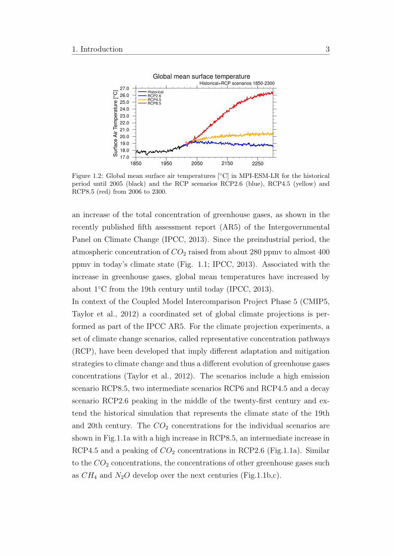
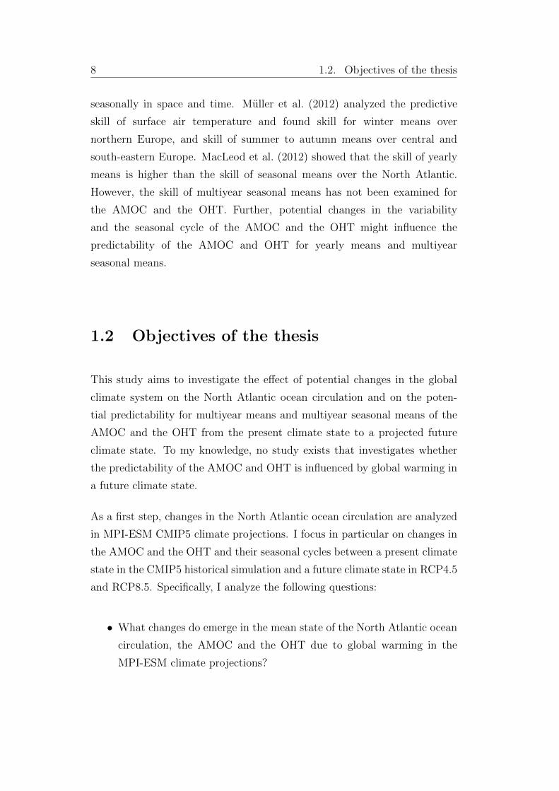
Figure 1.2: Global mean surface air temperatures [�C] in MPI-ESM-LR for the historicalperiod until 2005 (black) and the RCP scenarios RCP2.6 (blue), RCP4.5 (yellow) andRCP8.5 (red) from 2006 to 2300.
an increase of the total concentration of greenhouse gases, as shown in the
recently published fifth assessment report (AR5) of the Intergovernmental
Panel on Climate Change (IPCC, 2013). Since the preindustrial period, the
atmospheric concentration of CO2
raised from about 280 ppmv to almost 400
ppmv in today’s climate state (Fig. 1.1; IPCC, 2013). Associated with the
increase in greenhouse gases, global mean temperatures have increased by
about 1�C from the 19th century until today (IPCC, 2013).
In context of the Coupled Model Intercomparison Project Phase 5 (CMIP5,
Taylor et al., 2012) a coordinated set of global climate projections is per-
formed as part of the IPCC AR5. For the climate projection experiments, a
set of climate change scenarios, called representative concentration pathways
(RCP), have been developed that imply di↵erent adaptation and mitigation
strategies to climate change and thus a di↵erent evolution of greenhouse gases
concentrations (Taylor et al., 2012). The scenarios include a high emission
scenario RCP8.5, two intermediate scenarios RCP6 and RCP4.5 and a decay
scenario RCP2.6 peaking in the middle of the twenty-first century and ex-
tend the historical simulation that represents the climate state of the 19th
and 20th century. The CO2
concentrations for the individual scenarios are
shown in Fig.1.1a with a high increase in RCP8.5, an intermediate increase in
RCP4.5 and a peaking of CO2
concentrations in RCP2.6 (Fig.1.1a). Similar
to the CO2
concentrations, the concentrations of other greenhouse gases such
as CH4
and N2
O develop over the next centuries (Fig.1.1b,c).
4 1.1. Motivation
18
16
14
12
10
8
30
28
26
24
22
34
33
32
31
38
37
36
35
1850 1950 2050 2150 2250
Sea
surfa
ce te
mpe
ratu
re [°
C]
1850 1950 2050 2150 2250
1850 1950 2050 2150 22501850 1950 2050 2150 2250
Sea
surfa
ce te
mpe
ratu
re [°
C]
Sea
surfa
ce s
alin
itySe
a su
rface
sal
inity
SST - Subtropical gyre 20°N-40°N SSS - Subtropical gyre 20°N-40°N
SST - Subpolar gyre 40°N-60°N SSS - Subpolar gyre 40°N-60°N
a b
c d
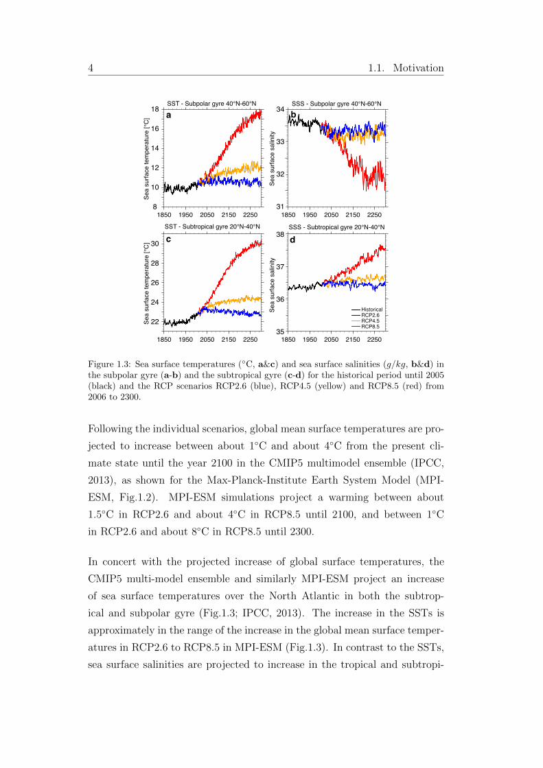
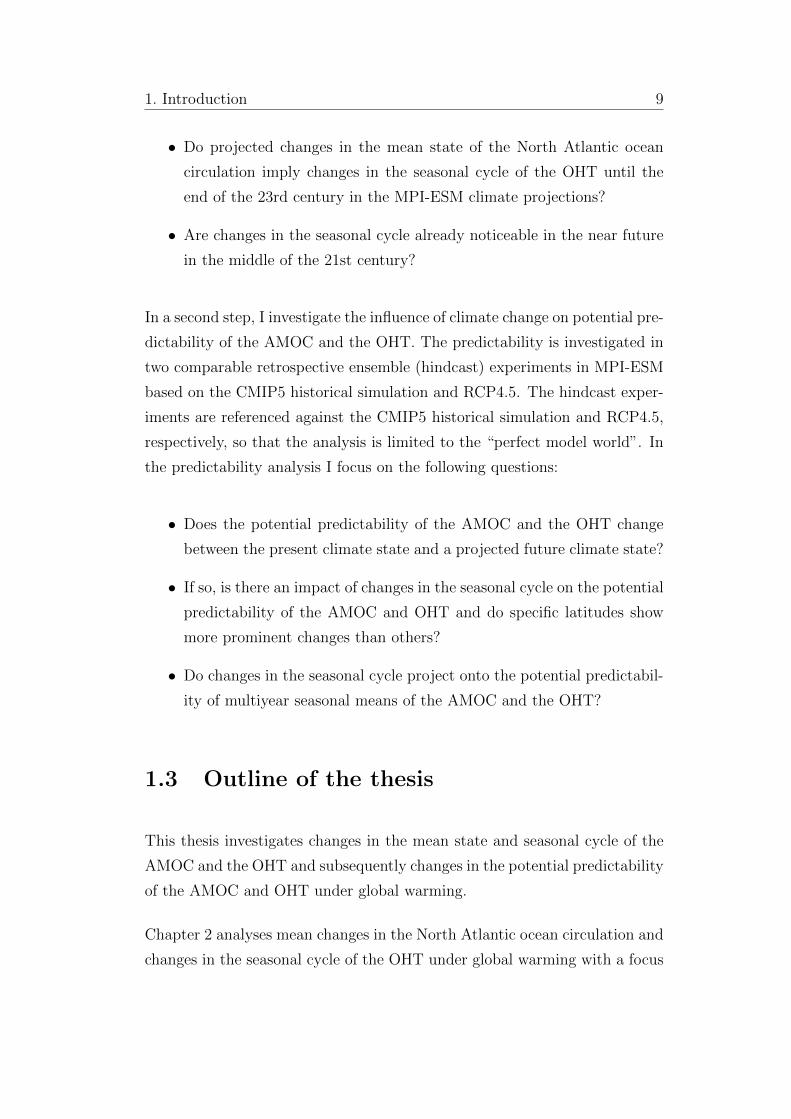
Figure 1.3: Sea surface temperatures (�C, a&c) and sea surface salinities (g/kg, b&d) inthe subpolar gyre (a-b) and the subtropical gyre (c-d) for the historical period until 2005(black) and the RCP scenarios RCP2.6 (blue), RCP4.5 (yellow) and RCP8.5 (red) from2006 to 2300.
Following the individual scenarios, global mean surface temperatures are pro-
jected to increase between about 1�C and about 4�C from the present cli-
mate state until the year 2100 in the CMIP5 multimodel ensemble (IPCC,
2013), as shown for the Max-Planck-Institute Earth System Model (MPI-
ESM, Fig.1.2). MPI-ESM simulations project a warming between about
1.5�C in RCP2.6 and about 4�C in RCP8.5 until 2100, and between 1�C
in RCP2.6 and about 8�C in RCP8.5 until 2300.
In concert with the projected increase of global surface temperatures, the
CMIP5 multi-model ensemble and similarly MPI-ESM project an increase
of sea surface temperatures over the North Atlantic in both the subtrop-
ical and subpolar gyre (Fig.1.3; IPCC, 2013). The increase in the SSTs is
approximately in the range of the increase in the global mean surface temper-
atures in RCP2.6 to RCP8.5 in MPI-ESM (Fig.1.3). In contrast to the SSTs,
sea surface salinities are projected to increase in the tropical and subtropi-
1. Introduction 5
cal North Atlantic, but to decrease in the subpolar North Atlantic (Fig.1.3;
IPCC, 2013). The freshening and warming of the subpolar North Atlantic in-
crease the buoyancy forcing and result in a reduction of convection and deep
water formation in the North Atlantic that is found to weaken the AMOC
(e.g., Gregory et al., 2005, Gregory and Tailleux, 2011, Weaver et al., 2012)
and accordingly to reduce the OHT.
Together with global warming, changes in the amplitude and phase of the
seasonal cycle of surface air temperatures (Dwyer et al., 2012) and accord-
ingly sea surface temperatures and sea surface salinities in the Arctic ocean
(Carton et al., 2015) are identified in climate projections. However, changes
in the seasonal cycle of the AMOC and the OHT due to global warming
which might impact the North Atlantic climate have not been investigated
to my knowledge.
1.1.2 Decadal predictability
The fundamental role of the AMOC and OHT for the North Atlantic cli-
mate and its variability (e.g., Sutton and Hodson, 2005, Knight et al., 2005,
Pohlmann et al., 2006) motivates to advance the understanding of the North
Atlantic climate predictability.
Decadal predictions are still in an early stage (Goddard et al., 2013), even
though a lot of progress and success was achieved in context of the recent
coordinated e↵ort of CMIP5 (Taylor et al., 2012, Meehl et al., 2014). In
CMIP5, decadal climate predictions have been investigated in a multi-model
framework based on retrospective ensemble forecast experiments, so-called
ensemble hindcast experiments (Meehl et al., 2009). Studies in the context
of CMIP5 mostly focussed on the analysis of the predictability under histori-
cal climate conditions that represent the climate state of the last half century
from 1960 to 2005. But studies invoking the impact of future climate change
on decadal predictability – in particular of the AMOC and the OHT – do not
exist to my knowledge apart from Boer (2009) who finds that the potential
(decadal) predictability of surface temperatures and precipitation is poten-
tially decreased under global warming and Tietsche et al. (2013) who find a
6 1.1. Motivation
a reduction in skill of Arctic sea ice predictions in the 21st century.
Following the work of Edward N. Lorenz, climate predictions can be classi-
fied into short-term (seasonal to inter-annual) forecasts and into long-term
climate projections over a few centuries (Lorenz, 1975). The former rely on
the knowledge of initial conditions which is never perfect. By errors in the
initial conditions, the forecast diverges from the true state of the system with
increasing lead time (initial value problem). The latter rely on the knowledge
of the external forcing, as for climate projections, and the exact initial con-
ditions become of second order (boundary value problem). Decadal climate
predictions range in between short-term forecasts and long-term climate pro-
jections with timescale of some years to several decades. Therefore, decadal
predictions rely on both, a good knowledge of the initial conditions for lead
times of a few years and the good knowledge of the external forcing for lead
times in the order of one decade or more and thus can be seen as a joint
initial and boundary value problem (e.g., Collins and Allen, 2002, Collins,
2002, Collins et al., 2006, Goddard et al., 2012). In contrast to numerical
weather prediction that aims to forecast most precisely individual weather
events, decadal climate prediction aims to provide information about the fu-
ture evolution of the statistics of mostly regional climate (e.g., Meehl et al.,
2014).
In the early stage of decadal predictions, studies were performed in so-called
“perfect model” experiments that compare the model hindcast against a con-
trol simulation in that model. Since continuous observations in the ocean,
especially of integrated quantities like the AMOC and the OHT, are sparse,
the validation of the prediction against a control simulation plays a crucial
role for the understanding of decadal predictability. These early studies found
predictability especially over the North Atlantic Ocean (Gri�es and Bryan,
1997, Pohlmann et al., 2004, Collins et al., 2006). Accordingly, more recent
predictability studies found the North Atlantic Ocean as a key region for
decadal predictions with distinct skill in predicting air and sea surface tem-
peratures (Pohlmann et al., 2009, van Oldenborgh et al., 2012, Matei et al.,
2012b, Pohlmann et al., 2013a), the North Atlantic heat content (Yeager
1. Introduction 7
et al., 2012, Kroger et al., 2012), the North Atlantic subpolar gyre (Matei
et al., 2012b, Yeager et al., 2012, Robson et al., 2012) or the Atlantic merid-
ional overturning circulation (Collins et al., 2006, Msadek et al., 2010, Matei
et al., 2012a, Pohlmann et al., 2013b).
Predictability is commonly estimated either from prognostic (classical) pre-
dictability or from potential (diagnostic) predictability (Latif et al., 2006).
Prognostic predictability is usually assessed from ensemble experiments by
perturbing the initial state and is often compared to the “perfect model” (e.g.,
Gri�es and Bryan, 1997, Collins, 2002, Pohlmann et al., 2006). Prognostic
predictability provides an upper limit of predictability in the model. Diagnos-
tic predictability is commonly estimated from the variance of the long-term
variability against internally generated variability which is not predictable
(e.g., Boer, 2004). The decadal predictability is usually estimated from one
or more of the following measures: The anomaly correlation coe�cent (ACC;
e.g., Collins, 2002) between the ensemble mean and the control simulation,
the prognostic potential predictability (e.g., Collins and Allen, 2002) that
compares the ensemble spread to the variance of the control simulation or
the root-mean-square error (e.g., Collins, 2002) showing deviations of the en-
semble hindcast from the control simulation. Recently, decadal predictability
has been estimated from reliability diagrams and the Brier Skill Score that
is routinely used in weather prediction and seasonal prediction (Corti et al.,
2012).
Studies on predictability of the AMOC have mostly focussed on one single
latitude. Recent studies analyzing the latitude-dependent predictability
showed, that the AMOC is potentially predictable with longer lead times in
the subtropical gyre than in the subpolar gyre (Tiedje et al., 2012, Bellucci
et al., 2013), while the predictability of the OHT tends to be longer in
the subpolar North Atlantic (Tiedje et al., 2012). Studies linking the
predictability of the AMOC and OHT are sparse (Tiedje and Baehr, 2014).
The majority of studies focussed on yearly means for the analysis of the
predictability. Nevertheless, the predictability might vary between di↵erent
seasons, as the parameters as well as the underlying mechanisms change
8 1.2. Objectives of the thesis
seasonally in space and time. Muller et al. (2012) analyzed the predictive
skill of surface air temperature and found skill for winter means over
northern Europe, and skill of summer to autumn means over central and
south-eastern Europe. MacLeod et al. (2012) showed that the skill of yearly
means is higher than the skill of seasonal means over the North Atlantic.
However, the skill of multiyear seasonal means has not been examined for
the AMOC and the OHT. Further, potential changes in the variability
and the seasonal cycle of the AMOC and the OHT might influence the
predictability of the AMOC and OHT for yearly means and multiyear
seasonal means.
1.2 Objectives of the thesis
This study aims to investigate the e↵ect of potential changes in the global
climate system on the North Atlantic ocean circulation and on the poten-
tial predictability for multiyear means and multiyear seasonal means of the
AMOC and the OHT from the present climate state to a projected future
climate state. To my knowledge, no study exists that investigates whether
the predictability of the AMOC and OHT is influenced by global warming in
a future climate state.
As a first step, changes in the North Atlantic ocean circulation are analyzed
in MPI-ESM CMIP5 climate projections. I focus in particular on changes in
the AMOC and the OHT and their seasonal cycles between a present climate
state in the CMIP5 historical simulation and a future climate state in RCP4.5
and RCP8.5. Specifically, I analyze the following questions:
• What changes do emerge in the mean state of the North Atlantic ocean
circulation, the AMOC and the OHT due to global warming in the
MPI-ESM climate projections?
1. Introduction 9
• Do projected changes in the mean state of the North Atlantic ocean
circulation imply changes in the seasonal cycle of the OHT until the
end of the 23rd century in the MPI-ESM climate projections?
• Are changes in the seasonal cycle already noticeable in the near future
in the middle of the 21st century?
In a second step, I investigate the influence of climate change on potential pre-
dictability of the AMOC and the OHT. The predictability is investigated in
two comparable retrospective ensemble (hindcast) experiments in MPI-ESM
based on the CMIP5 historical simulation and RCP4.5. The hindcast exper-
iments are referenced against the CMIP5 historical simulation and RCP4.5,
respectively, so that the analysis is limited to the “perfect model world”. In
the predictability analysis I focus on the following questions:
• Does the potential predictability of the AMOC and the OHT change
between the present climate state and a projected future climate state?
• If so, is there an impact of changes in the seasonal cycle on the potential
predictability of the AMOC and OHT and do specific latitudes show
more prominent changes than others?
• Do changes in the seasonal cycle project onto the potential predictabil-
ity of multiyear seasonal means of the AMOC and the OHT?
1.3 Outline of the thesis
This thesis investigates changes in the mean state and seasonal cycle of the
AMOC and the OHT and subsequently changes in the potential predictability
of the AMOC and OHT under global warming.
Chapter 2 analyses mean changes in the North Atlantic ocean circulation and
changes in the seasonal cycle of the OHT under global warming with a focus
10 1.3. Outline of the thesis
on the RCP8.5 scenario in MPI-ESM for long-term changes until the end of
the 23rd century. Section 2.1 is written in paper form and is submitted to
Journal of Climate.1 This chapter focusses on the mechanisms that drive
changes in the OHT and its seasonal cycle in the climate projection. Section
2.2 provides an analysis of the OHT seasonal cycle based on a heat function
in potential temperature coordinates.
Chapter 3 investigates changes in the AMOC and OHT seasonal cycle until
the middle of the 21st century. As a prerequisite for the potential predictabil-
ity analysis, I identify latitudes with considerable changes in the seasonal
cycle that might imply considerable changes in the potential predictability of
AMOC and the OHT.
Chapter 4 investigates whether global climate change impacts the potential
predictability of the AMOC and the OHT from a present climate state repre-
sented by the CMIP5 historical simulation to a future climate state in RCP4.5
in the middle of the 21st century.
Chapter 5 gives an overall summary of the results and conclusions of the
thesis.
1This section is submitted to Journal of Climate as Fischer et al. (2015): The Atlanticmeridional heat transport seasonal cycle in a MPI-ESM climate projection.
2 Long-term changes in the At-
lantic meridional heat trans-
port and its seasonal cycle
2.1 The Atlantic meridional heat transport
seasonal cycle in a MPI-ESM climate pro-
jection1
Abstract
We investigate the e↵ect of a projected reduction in the Atlantic Ocean
meridional heat transport (OHT) on changes in its seasonal cycle. We
analyze a climate projection experiment with the Max-Planck Institute
Earth System Model (MPI-ESM) performed for the Coupled Model
Intercomparison Project phase 5 (CMIP5). In the RCP8.5 climate
change scenario, the oceanic OHT declines in MPI-ESM in the North
Atlantic by 30-50% by the end of the 23rd century. The decline in the
OHT is accompanied by a change in the seasonal cycle of the total
OHT and its components. We decompose the OHT into overturning
and gyre component, and analyze changes in the vertical structure
1This section is submitted to Journal of Climate as Fischer et al. (2015): The Atlanticmeridional heat transport seasonal cycle in a MPI-ESM climate projection.
12 2.1. The OHT seasonal cycle in a MPI-ESM climate projection
of the OHT seasonal cycle in individual water masses. For the total
OHT seasonal cycle, we find a northward shift of 5 degrees and latitude
dependent temporal shifts of 1 to 6 months that are mainly associated
with changes in the meridional velocity field. We find that the shift
in the OHT seasonal cycle predominantly results from changes in the
wind-driven surface and intermediate circulation which project onto
the overturning component of the OHT in the tropical and subtropical
North Atlantic. This leads to latitude dependent shifts of 1 to 6 months
in the overturning component. In the subpolar North Atlantic, we
find that the reduction of the North Atlantic Deep Water formation in
RCP8.5 results in a strongly weakened seasonal cycle in North Atlantic
Deep Water with an almost absent seasonal amplitude by the end of
the 23rd century.
2.1.1 Introduction
Global surface temperatures are projected to warm - depending on the con-
sidered climate change scenario - intensively over the next centuries (IPCC,
2013) accompanied by a projected shift in the amplitude and phase of the
seasonal cycle of surface air temperatures (Dwyer et al., 2012). In concert,
the Atlantic meridional overturning circulation (AMOC) is projected to slow
down (Weaver et al., 2012, IPCC, 2013) and thus the associated Atlantic
Ocean meridional heat transport (OHT) due to their direct linear relation
found in observations and model studies (Johns et al., 2011, Msadek et al.,
2013). However, it is unclear how climate change along with a projected
shift in the seasonal cycle of surface temperatures a↵ects the seasonal cycle
of the ocean circulation, and especially of the OHT. Here, we investigate
projected changes in the OHT seasonal cycle in a Coupled Model Intercom-
parison Project phase 5 (CMIP5) climate projection (Taylor et al., 2012)
performed in the global coupled Max-Planck Institute Earth System Model
(MPI-ESM) .
In the CMIP5 Representative Concentration Pathway (RCP) RCP8.5, sur-
face air temperatures are expected to increase by about 8 degrees in the global
2. Long-term changes in the OHT and its seasonal cycle 13
mean until the year 2300 in the CMIP5 multi-model ensemble (IPCC, 2013).
The warming manifests itself over the continents and in particular in polar
regions where an increase in surface temperatures of more than 20�C arises
in climate projections until 2300 (e.g., IPCC, 2013, Bintanja and Van der
Linden, 2013). Due to the strong warming in polar latitudes the meridional
temperature gradient from the equator to the poles is also strongly reduced
in the Northern Hemisphere. The atmospheric circulation patterns are pro-
jected to move poleward in concert with the warming of surface temperature,
leading to a poleward expansion of the tropical cell and a poleward shift of
the jet stream and storm track (Chang et al., 2012, Hu et al., 2013, IPCC,
2013). In contrast to the general warming, the surface air temperatures show
a prominent area of reduced warming over the North Atlantic subpolar gyre
(SPG) in the set of CMIP5 climate projections associated with an adjust-
ment of the Atlantic meridional overturning circulation (AMOC) (Drijfhout
et al., 2012) or a reduction of the OHT into the SPG (Rahmstorf et al., 2015).
These changes in the surface temperature patterns thus suggest considerable
changes in the North Atlantic ocean circulation, the AMOC and the associ-
ated OHT.
The implications of the Atlantic ocean circulation and the OHT for the North
Atlantic sector and the European climate have been widely discussed. The
AMOC and OHT in the North Atlantic has been shown to a↵ect the North
Atlantic heat content and the North Atlantic sea surface temperatures (SST;
e.g., Dong and Sutton, 2003, Grist et al., 2010, Sonnewald et al., 2013, Muir
and Fedorov, 2014). Changes in the North Atlantic SSTs and the air-sea
interaction appear to be important for influencing the atmospheric circula-
tion, the multidecadal variability of the North Atlantic sector an the North
American and European climate on inter-annual to multi-decadal time scales
(Rodwell et al., 2004, Sutton and Hodson, 2005, Gastineau and Frankignoul,
2015).
Further, a response of the NAO to North Atlantic sea surface temperatures
has been found both in observations and model studies (Czaja et al., 1999,
Czaja and Frankignoul, 2002, Rodwell and Folland, 2002, Frankignoul et al.,
2013, Gastineau et al., 2013, Gastineau and Frankignoul, 2015). Via the
Atlantic Multidecadal Oscillation (AMO), which is thought to result from
14 2.1. The OHT seasonal cycle in a MPI-ESM climate projection
AMOC and OHT variability (e.g., Delworth and Greatbatch, 2000, Knight
et al., 2005, Msadek and Frankignoul, 2009, Zhang and Wang, 2013), the SST
variability has been linked to a number of climate phenomena, such as Sahel
rainfall, Atlantic hurricane activity and North American and European sum-
mer climate (Enfield et al., 2001, Sutton and Hodson, 2005, Knight et al.,
2006, Zhang and Delworth, 2006, Sutton and Dong, 2012). However, the
specific role and direct importance of the OHT for European climate is still
controversially discussed and the exact mechanism not fully understood (Bry-
den, 1993, Seager et al., 2002, Rhines et al., 2008, Riser and Lozier, 2013).
For the seasonal variability, the coupling between ocean and atmosphere is
less understood. Minobe et al. (2010) have shown an atmospheric response
to Gulf stream variability with seasonal variations. When considering also
the impact of seasonal variations in the total OHT on European climate, the
relation becomes even more complex and thus requires a better understand-
ing of the OHT and its coupling to the atmosphere.
Yet, most of the present understanding stems from model analysis, due to a
lack of continuous observations. Most traditional observations of the OHT
are based on hydrographic snapshots (e.g., Bryan, 1962, Hall and Bryden,
1982, Lavin et al., 1998, Lumpkin and Speer, 2007) or inverse methods (e.g.,
Macdonald and Wunsch, 1996, Ganachaud and Wunsch, 2000, 2003) and give
estimates of the time mean OHT of about 1 PW, but do not describe the
OHT variability. Further, single hydrographic snapshots may be a↵ected by
a seasonal bias due to the predominance of field work during summer. Re-
cently, the two time series of the 26�N Rapid array and observations at 41�N
have indicated long-term variability and a clear seasonal cycle of the OHT in
the North Atlantic (Johns et al., 2011, Hobbs and Willis, 2012).
A better understanding of the dynamics of the seasonal cycle of the OHT has
been gained from a number of model studies. The pioneering study by Bryan
(1982b) used a global ocean circulation model forced with observed winds.
Bryan pointed out the importance of the wind-driven Ekman mass transport
and of the associated Ekman heat transport for driving the seasonal vari-
ability of the OHT, which was also found in subsequent studies (Sarmiento,
1986, Lee and Marotzke, 1998, Jayne and Marotzke, 2001, Boning et al.,
2001, Cabanes et al., 2008, Balan Sarojini et al., 2011, Munoz et al., 2011).
2. Long-term changes in the OHT and its seasonal cycle 15
Bryan argued that changes in the zonally integrated wind stress, leading to
changes in the Ekman mass transport, are balanced by a barotropic return
flow. Jayne and Marotzke (2001) provided the theoretical and dynamical
justification for Bryan’s argumentation, stressing again the important role of
the Ekman transport for the seasonal cycle of the OHT.
Traditionally, the OHT is decomposed into a vertical overturning component,
which is commonly linked to the large scale overturning, and a horizontal gyre
component giving correlations of the zonal deviations of the velocity and tem-
perature field (Bryan, 1962, 1982a, Bryden and Imawaki, 2001, Siedler et al.,
2013). The gyre component is commonly linked to the horizontal gyre cir-
culation and contributions from the eddy field. Previous studies have shown
that the overturning component dominates the time mean, as well as the
interdecadal variability of the OHT in the tropical and subtropical North At-
lantic, whereas the overturning and gyre component contribute about equally
to the OHT and its interdecadal variability in the subpolar North Atlantic
(e.g., Eden and Jung, 2001). But this decomposition does not reveal the ver-
tical structure of the OHT and contributions from individual water masses.
Hence, recent studies have attempted to determine the vertical pathways of
the OHT in observations and model studies. Talley (2003) has analyzed the
vertical pathways of the OHT in observations. She found that 60% of the
mean OHT at 24�N in the North Atlantic results from the intermediate and
deep overturning, while the remaining 40% are carried northward in a shallow
overturning layer, in contrast to the traditional view, where about 90% of the
heat transport are ascribed to the deep overturning circulation (e.g. Bryden
and Imawaki, 2001).
Boccaletti et al. (2005) and Ferrari and Ferreira (2011) analyzed the verti-
cal structure of the heat transport based on a heat function in depth and
temperature coordinates. Boccaletti et al. (2005) touched the problem of re-
circulation cells that complicate the calculation of the heat function in depth
coordinates. Ferrari and Ferreira (2011) circumvented the problem of recir-
culation cells by calculating the heat function in temperature coordinates.
They showed that the OHT is surface intensified and follows from a com-
bined circulation of cold and warm water masses, so that most of the heat
transport cannot be assigned to shallow or deep circulations only. However,
16 2.1. The OHT seasonal cycle in a MPI-ESM climate projection
the impact of changes in the vertical structure of the OHT on its seasonal
cycle is still unclear.
With this study, we aim to understand how the Atlantic Ocean meridional
heat transport seasonal cycle is a↵ected by global warming and what deter-
mines potential changes in the OHT seasonal cycle. For our analysis, we use
a CMIP5 climate change projection performed in MPI-ESM, with a focus
on the climate change scenario RCP8.5 with the strongest climate change
forcing involved. We aim to identify changes in the seasonal cycle of Atlantic
meridional heat transport and its sources including changes in the circulation
of the surface and upper ocean and changes in the deep circulation. Second,
to analyze di↵erent physical mechanisms that contribute to the changes in
the seasonal cycle, we look at the individual contributions to the total OHT
on seasonal time scales. Therefore, we first decompose the OHT into gyre-
and overturning component, related to the horizontal gyre circulation and to
the overturning circulation in the North Atlantic and consider changes in the
wind-driven Ekman heat transport. To analyze the vertical structure of the
OHT and the relative contributions of various depths to the seasonal cycle,
we investigate the vertical structure of OHT in density coordinates.
This study is structured as follows: first, we describe the analyzed CMIP5 ex-
periments performed in the coupled climate model MPI-ESM and the Atlantic
meridional heat transport and its decomposition (section 2.1.2). Section 2.1.3
presents mean changes in the AMOC and of the OHT in the climate projec-
tion under global warming and the main characteristics of the OHT and its
components in MPI-ESM. In section 2.1.4 we analyze the changes in the
seasonal cycle of the OHT and its components in the MPI-ESM climate pro-
jections for long-term changes by the end of the 23rd century. A discussion
and conclusions are given in sections 2.1.5 and 2.1.6.
2. Long-term changes in the OHT and its seasonal cycle 17
2.1.2 Model and Methods
2.1.2.1 The CMIP5 climate change scenario RCP8.5 in MPI-ESM
We analyze one member of the CMIP5 ensemble (Taylor et al., 2012) per-
formed in the coupled Max-Planck-Institute Earth System model in low reso-
lution configuration (MPI-ESM-LR) that is integrated from 1850 to 2300. In
the ocean component MPIOM (Marsland et al., 2003, Jungclaus et al., 2013),
the horizontal resolution is 1.5 degree on average with 40 unevenly spaced
vertical levels. The atmospheric component ECHAM6 (Stevens et al., 2013)
has a horizontal resolution of T63 and includes 47 vertical levels.
We focus on one member the CMIP5 ensemble in the historical simulation
(1850-2005) and extend the historical simulation with the Representative
Concentration Pathway (RCP) RCP8.5 from 2006 to 2300. In RCP8.5, a
rising radiative forcing following “business as usual” is applied, which rises
to 8.5W/m2 in the year 2100, and further increases after that (van Vuuren
et al., 2011). We focus on longterm changes in RCP8.5, comparing the period
1850-1950 for the historical simulation (HISTmean) to the period 2200-2300
for the RCP8.5 scenario (RCPmean), where we expect the strongest changes
in the North Atlantic ocean circulation and in the seasonal cycle of the OHT.
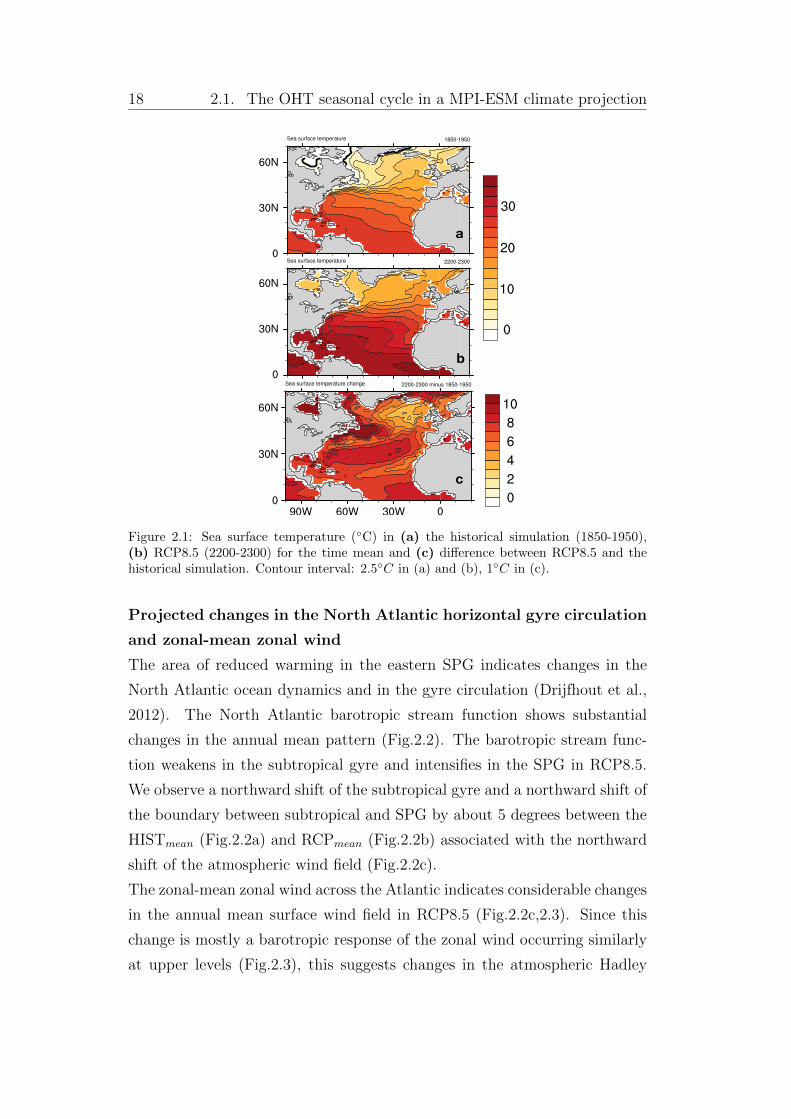
Projected changes in the North Atlantic sea surface temperatures
In concert with the projected warming of surface air temperatures, the sea
surface temperatures (SST) are projected to warm globally and also in the
North Atlantic sector in RCP8.5 (Fig.2.1). A similar “warming hole” sig-
nature as found for surface air temperatures (c.f., Drijfhout et al., 2012) is
present in the North Atlantic SSTs (Fig.2.1) with a stronger warming in
polar regions and an area of reduced warming in the SPG (Fig.2.1c). Pro-
nounced regional variations of the SST change suggest important changes in
the North Atlantic ocean circulation and its dynamics. The SST front along
the Gulf Stream path shifts northward and weakens which might also impact
the North Atlantic storm track as already shown for the current climate state
(e.g. Minobe et al., 2008, 2010, Hand et al., 2014).
18 2.1. The OHT seasonal cycle in a MPI-ESM climate projection
Figure 2.1: Sea surface temperature (�C) in (a) the historical simulation (1850-1950),(b) RCP8.5 (2200-2300) for the time mean and (c) di↵erence between RCP8.5 and thehistorical simulation. Contour interval: 2.5�C in (a) and (b), 1�C in (c).
Projected changes in the North Atlantic horizontal gyre circulation
and zonal-mean zonal wind
The area of reduced warming in the eastern SPG indicates changes in the
North Atlantic ocean dynamics and in the gyre circulation (Drijfhout et al.,
2012). The North Atlantic barotropic stream function shows substantial
changes in the annual mean pattern (Fig.2.2). The barotropic stream func-
tion weakens in the subtropical gyre and intensifies in the SPG in RCP8.5.
We observe a northward shift of the subtropical gyre and a northward shift of
the boundary between subtropical and SPG by about 5 degrees between the
HISTmean (Fig.2.2a) and RCPmean (Fig.2.2b) associated with the northward
shift of the atmospheric wind field (Fig.2.2c).
The zonal-mean zonal wind across the Atlantic indicates considerable changes
in the annual mean surface wind field in RCP8.5 (Fig.2.2c,2.3). Since this
change is mostly a barotropic response of the zonal wind occurring similarly
at upper levels (Fig.2.3), this suggests changes in the atmospheric Hadley
2. Long-term changes in the OHT and its seasonal cycle 19
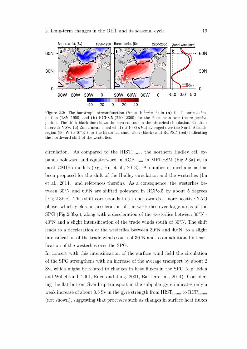
Figure 2.2: The barotropic streamfunction (Sv = 106m3s�1) in (a) the historical sim-ulation (1850-1950) and (b) RCP8.5 (2200-2300) for the time mean over the respectiveperiod. The thick black line shows the zero contour in the historical simulation. Contourinterval: 5 Sv. (c) Zonal mean zonal wind (at 1000 hPa) averaged over the North Atlanticregion (90�W to 10�E ) for the historical simulation (black) and RCP8.5 (red) indicatingthe northward shift of the westerlies.
circulation. As compared to the HISTmean, the northern Hadley cell ex-
pands poleward and equatorward in RCPmean in MPI-ESM (Fig.2.3a) as in
most CMIP5 models (e.g., Hu et al., 2013). A number of mechanisms has
been proposed for the shift of the Hadley circulation and the westerlies (Lu
et al., 2014, and references therein). As a consequence, the westerlies be-
tween 30�N and 60�N are shifted poleward in RCP8.5 by about 5 degrees
(Fig.2.3b,c). This shift corresponds to a trend towards a more positive NAO
phase, which yields an acceleration of the westerlies over large areas of the
SPG (Fig.2.3b,c), along with a deceleration of the westerlies between 30�N -
40�N and a slight intensification of the trade winds south of 30�N. The shift
leads to a deceleration of the westerlies between 30�N and 40�N, to a slight
intensification of the trade winds south of 30�N and to an additional intensi-
fication of the westerlies over the SPG.
In concert with this intensification of the surface wind field the circulation
of the SPG strengthens with an increase of the average transport by about 2
Sv, which might be related to changes in heat fluxes in the SPG (e.g. Eden
and Willebrand, 2001, Eden and Jung, 2001, Barrier et al., 2014). Consider-
ing the flat-bottom Sverdrup transport in the subpolar gyre indicates only a
weak increase of about 0.5 Sv in the gyre strength from HISTmean to RCPmean
(not shown), suggesting that processes such as changes in surface heat fluxes
20 2.1. The OHT seasonal cycle in a MPI-ESM climate projection
c
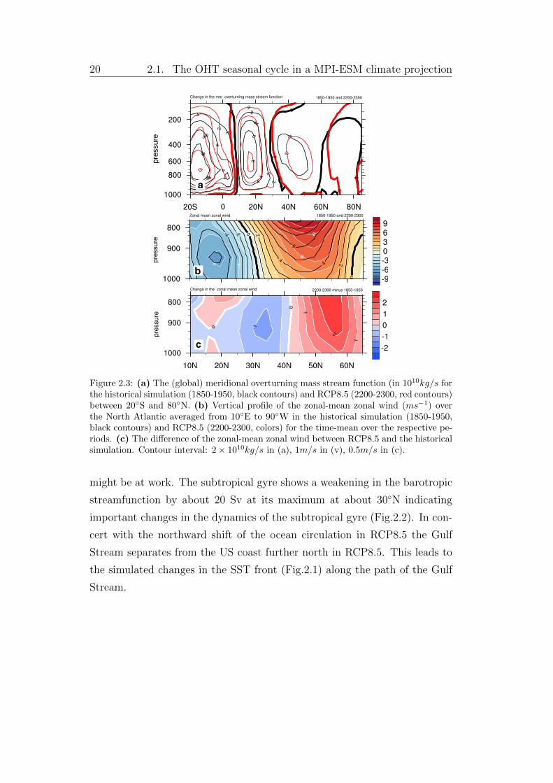
a
Figure 2.3: (a) The (global) meridional overturning mass stream function (in 1010kg/s forthe historical simulation (1850-1950, black contours) and RCP8.5 (2200-2300, red contours)between 20�S and 80�N. (b) Vertical profile of the zonal-mean zonal wind (ms�1) overthe North Atlantic averaged from 10�E to 90�W in the historical simulation (1850-1950,black contours) and RCP8.5 (2200-2300, colors) for the time-mean over the respective pe-riods. (c) The di↵erence of the zonal-mean zonal wind between RCP8.5 and the historicalsimulation. Contour interval: 2⇥ 1010kg/s in (a), 1m/s in (v), 0.5m/s in (c).
might be at work. The subtropical gyre shows a weakening in the barotropic
streamfunction by about 20 Sv at its maximum at about 30�N indicating
important changes in the dynamics of the subtropical gyre (Fig.2.2). In con-
cert with the northward shift of the ocean circulation in RCP8.5 the Gulf
Stream separates from the US coast further north in RCP8.5. This leads to
the simulated changes in the SST front (Fig.2.1) along the path of the Gulf
Stream.
2. Long-term changes in the OHT and its seasonal cycle 21
2.1.2.2 The Atlantic meridional heat transport and its decompo-
sition
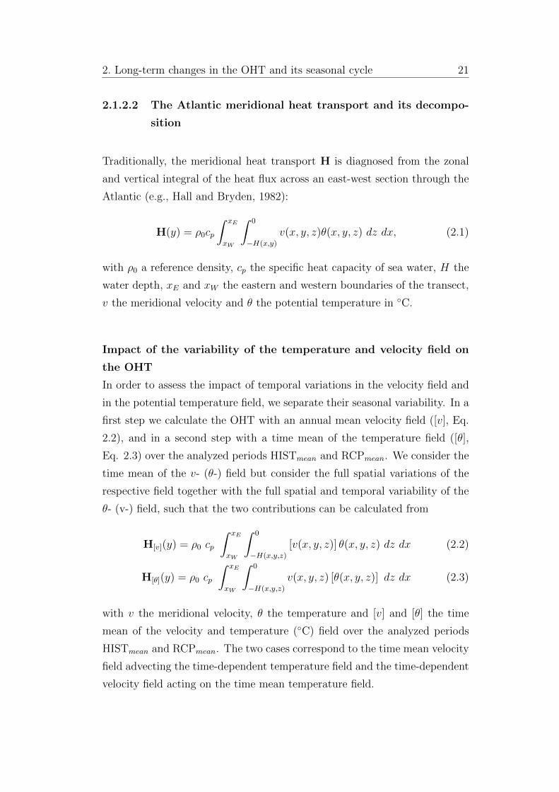
Traditionally, the meridional heat transport H is diagnosed from the zonal
and vertical integral of the heat flux across an east-west section through the
Atlantic (e.g., Hall and Bryden, 1982):
H(y) = ⇢0
cp
Z xE
xW
Z0
�H(x,y)
v(x, y, z)✓(x, y, z) dz dx, (2.1)
with ⇢0
a reference density, cp the specific heat capacity of sea water, H the
water depth, xE and xW the eastern and western boundaries of the transect,
v the meridional velocity and ✓ the potential temperature in �C.
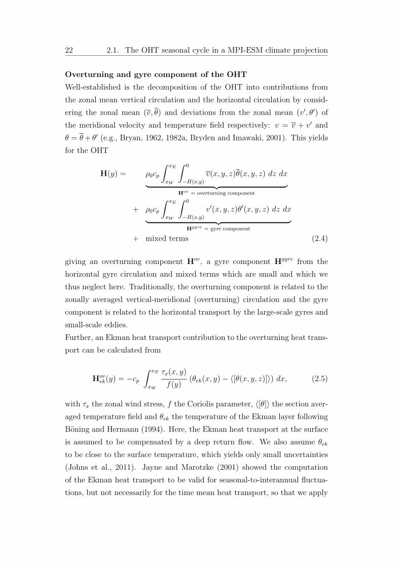
Impact of the variability of the temperature and velocity field on
the OHT
In order to assess the impact of temporal variations in the velocity field and
in the potential temperature field, we separate their seasonal variability. In a
first step we calculate the OHT with an annual mean velocity field ([v], Eq.
2.2), and in a second step with a time mean of the temperature field ([✓],
Eq. 2.3) over the analyzed periods HISTmean and RCPmean. We consider the
time mean of the v- (✓-) field but consider the full spatial variations of the
respective field together with the full spatial and temporal variability of the
✓- (v-) field, such that the two contributions can be calculated from
H[v](y) = ⇢
0
cp
Z xE
xW
Z0
�H(x,y,z)
[v(x, y, z)] ✓(x, y, z) dz dx (2.2)
H[✓](y) = ⇢
0
cp
Z xE
xW
Z0
�H(x,y,z)
v(x, y, z) [✓(x, y, z)] dz dx (2.3)
with v the meridional velocity, ✓ the temperature and [v] and [✓] the time
mean of the velocity and temperature (�C) field over the analyzed periods
HISTmean and RCPmean. The two cases correspond to the time mean velocity
field advecting the time-dependent temperature field and the time-dependent
velocity field acting on the time mean temperature field.
22 2.1. The OHT seasonal cycle in a MPI-ESM climate projection
Overturning and gyre component of the OHT
Well-established is the decomposition of the OHT into contributions from
the zonal mean vertical circulation and the horizontal circulation by consid-
ering the zonal mean (v, ✓) and deviations from the zonal mean (v0, ✓0) of
the meridional velocity and temperature field respectively: v = v + v0 and
✓ = ✓+ ✓0 (e.g., Bryan, 1962, 1982a, Bryden and Imawaki, 2001). This yields
for the OHT
H(y) = ⇢0
cp
Z xE
xW
Z0
�H(x,y)
v(x, y, z)✓(x, y, z) dz dx
| {z }Hov
= overturning component
+ ⇢0
cp
Z xE
xW
Z0
�H(x,y)
v0(x, y, z)✓0(x, y, z) dz dx
| {z }Hgyre
= gyre component
+ mixed terms (2.4)
giving an overturning component Hov, a gyre component Hgyre from the
horizontal gyre circulation and mixed terms which are small and which we
thus neglect here. Traditionally, the overturning component is related to the
zonally averaged vertical-meridional (overturning) circulation and the gyre
component is related to the horizontal transport by the large-scale gyres and
small-scale eddies.
Further, an Ekman heat transport contribution to the overturning heat trans-
port can be calculated from
Hovek(y) = �cp
Z xE
xW
⌧x(x, y)
f(y)(✓ek(x, y)� h[✓(x, y, z)]i) dx, (2.5)
with ⌧x the zonal wind stress, f the Coriolis parameter, h[✓]i the section aver-
aged temperature field and ✓ek the temperature of the Ekman layer following
Boning and Hermann (1994). Here, the Ekman heat transport at the surface
is assumed to be compensated by a deep return flow. We also assume ✓ek
to be close to the surface temperature, which yields only small uncertainties
(Johns et al., 2011). Jayne and Marotzke (2001) showed the computation
of the Ekman heat transport to be valid for seasonal-to-interannual fluctua-
tions, but not necessarily for the time mean heat transport, so that we apply
2. Long-term changes in the OHT and its seasonal cycle 23
the Ekman transport calculation only to the OHT seasonal variability.
2.1.2.3 The vertical structure of the Atlantic meridional heat
transport
To investigate the vertical structure of the OHT, we calculate the OHT in
potential density classes, similar to the analysis of Talley (2003). We subdi-
vide the water masses into surface, intermediate, North Atlantic Deep Water
(NADW) and abyssal waters from the Antarctic Bottom Water (AABW).
For this purpose, we define individual water masses relative to 26�N in the
model based on a regression analysis of potential temperature ✓ and salinity
S at 26�N on the AMOC at 26�N following Baehr et al. (2007). We perform
the regression analysis for eastern boundary fields, western boundary fields
and the zonal mean fields of ✓ and S for HISTmean and RCPmean individually.
The regression analysis enables us to identify main water masses based on
changes in the vertical profiles of the regression on the AMOC. In contrast
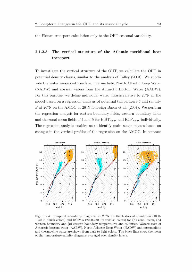
Figure 2.4: Temperature-salinity diagrams at 26�N for the historical simulation (1850-1950 in bluish colors) and RCP8.5 (2200-2300 in reddish colors) for (a) zonal mean, (b)western boundary and (c) eastern boundary temperatures and salinities. Watermasses ofAntarctic bottom water (AABW), North Atlantic Deep Water (NADW) and intermediateand thermocline water are shown from dark to light colors. The black lines show the meanof the temperature-salinity diagrams averaged over density layers.
24 2.1. The OHT seasonal cycle in a MPI-ESM climate projection
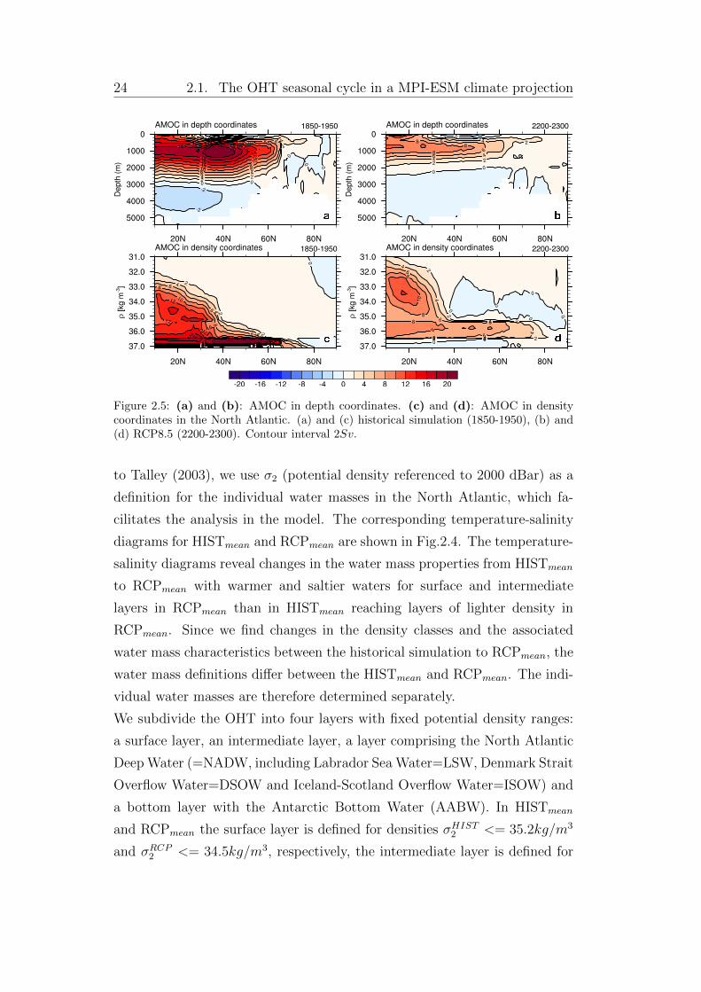
1850-1950
1850-1950 2200-2300
2200-2300
Figure 2.5: (a) and (b): AMOC in depth coordinates. (c) and (d): AMOC in densitycoordinates in the North Atlantic. (a) and (c) historical simulation (1850-1950), (b) and(d) RCP8.5 (2200-2300). Contour interval 2Sv.
to Talley (2003), we use �2
(potential density referenced to 2000 dBar) as a
definition for the individual water masses in the North Atlantic, which fa-
cilitates the analysis in the model. The corresponding temperature-salinity
diagrams for HISTmean and RCPmean are shown in Fig.2.4. The temperature-
salinity diagrams reveal changes in the water mass properties from HISTmean
to RCPmean with warmer and saltier waters for surface and intermediate
layers in RCPmean than in HISTmean reaching layers of lighter density in
RCPmean. Since we find changes in the density classes and the associated
water mass characteristics between the historical simulation to RCPmean, the
water mass definitions di↵er between the HISTmean and RCPmean. The indi-
vidual water masses are therefore determined separately.
We subdivide the OHT into four layers with fixed potential density ranges:
a surface layer, an intermediate layer, a layer comprising the North Atlantic
DeepWater (=NADW, including Labrador SeaWater=LSW, Denmark Strait
Overflow Water=DSOW and Iceland-Scotland Overflow Water=ISOW) and
a bottom layer with the Antarctic Bottom Water (AABW). In HISTmean
and RCPmean the surface layer is defined for densities �HIST2
<= 35.2kg/m3
and �RCP2
<= 34.5kg/m3, respectively, the intermediate layer is defined for
2. Long-term changes in the OHT and its seasonal cycle 25
densities 35.2kg/m3 < �HIST2
<= 35.8kg/m3 and 34.5kg/m3 < �RCP2
<=
36.61kg/m3, respectively, the NADW is defined for densities 35.8kg/m3 <
�HIST2
<= 36.91kg/m3 and 36.61kg/m3 < �RCP2
<= 36.91kg/m3, respec-
tively, and the AABW is defined for densities �HIST2
> 35.8kg/m3 and
�RCP2
> 36.91kg/m3, respectively. For each density range, we then calcu-
late the heat fluxes and the corresponding seasonal cycles. In RCP8.5, the
deep water formation in the North Atlantic is significantly reduced, leading
to a change in the water mass distribution. In RCP8.5, it is not convenient
anymore to define a traditional North Atlantic Deep Water, which is why
the density classes used to define the individual water masses di↵er between
the historical simulation and RCP8.5. A finer separation of individual water
masses is not feasible in the model.
2.1.3 Mean changes in the Atlantic meridional over-
turning circulation and meridional heat trans-
port
2.1.3.1 AMOC
The mean changes seen in the SSTs, the surface wind field and in the North
Atlantic ocean and gyre circulation influence the AMOC and the meridional
heat transport, which we focus on in the remainder of the study. The
AMOC shows significant changes in the time mean from HISTmean to
RCPmean (Fig.2.5). The AMOC calculated in depth coordinates shows that
the northward overturning cell is reduced and shifted to the surface from
the HISTmean to RCPmean (Fig.2.5a,b). The maximum of the stream
function given by (y, z) =0Rz
xER
xW
v(x, y, z) dx dz commonly used as an
index for the AMOC, is substantially reduced by 30 to 50% from HISTmean
to RCPmean (Fig.2.5a,b;Fig.2.6a).
Considering the AMOC in density coordinates (Fig.2.5c,d) indicates a
similar surfaceward shift of the AMOC cell to layers of lower density from
HISTmean to RCPmean (Fig.2.5c,d). We find only a slight decrease of the
26 2.1. The OHT seasonal cycle in a MPI-ESM climate projection
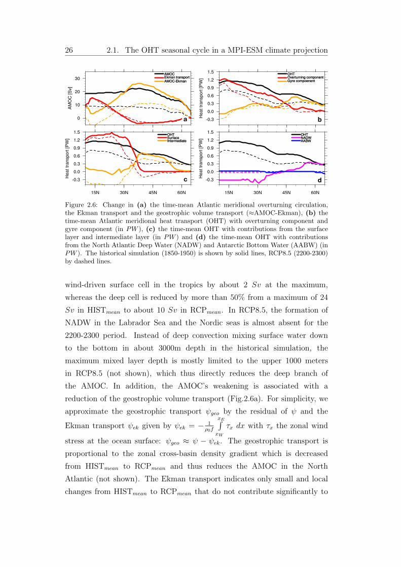
d
Figure 2.6: Change in (a) the time-mean Atlantic meridional overturning circulation,the Ekman transport and the geostrophic volume transport (⇡AMOC-Ekman), (b) thetime-mean Atlantic meridional heat transport (OHT) with overturning component andgyre component (in PW ), (c) the time-mean OHT with contributions from the surfacelayer and intermediate layer (in PW ) and (d) the time-mean OHT with contributionsfrom the North Atlantic Deep Water (NADW) and Antarctic Bottom Water (AABW) (inPW ). The historical simulation (1850-1950) is shown by solid lines, RCP8.5 (2200-2300)by dashed lines.
wind-driven surface cell in the tropics by about 2 Sv at the maximum,
whereas the deep cell is reduced by more than 50% from a maximum of 24
Sv in HISTmean to about 10 Sv in RCPmean. In RCP8.5, the formation of
NADW in the Labrador Sea and the Nordic seas is almost absent for the
2200-2300 period. Instead of deep convection mixing surface water down
to the bottom in about 3000m depth in the historical simulation, the
maximum mixed layer depth is mostly limited to the upper 1000 meters
in RCP8.5 (not shown), which thus directly reduces the deep branch of
the AMOC. In addition, the AMOC’s weakening is associated with a
reduction of the geostrophic volume transport (Fig.2.6a). For simplicity, we
approximate the geostrophic transport geo by the residual of and the
Ekman transport ek given by ek = � 1
⇢0f
xER
xW
⌧x dx with ⌧x the zonal wind
stress at the ocean surface: geo ⇡ � ek. The geostrophic transport is
proportional to the zonal cross-basin density gradient which is decreased
from HISTmean to RCPmean and thus reduces the AMOC in the North
Atlantic (not shown). The Ekman transport indicates only small and local
changes from HISTmean to RCPmean that do not contribute significantly to
2. Long-term changes in the OHT and its seasonal cycle 27
the weakening of the AMOC (Fig.2.6a).
2.1.3.2 OHT
Similar to the AMOC, the RCP8.5 scenario reveals considerable changes in
the associated OHT. For RCPmean, the OHT shows a pronounced weakening
by 30-50% from about 1.2 PW to about 0.8 PW between 10�N and 30�N
and from about 0.8 PW to about 0.4P W between 40�N and 55�N by the
end of the 23rd century (Fig.2.6b). The reduction in the total OHT in the
subtropical North Atlantic can be attributed almost entirely to a reduction
in the overturning heat transport, while changes in the gyre component are
comparably small. Only in the SPG, the gyre component also indicates a
substantial weakening, so that both the overturning and the gyre component
contribute to the reduction in the total heat transport in the subpolar North
Atlantic. The reduction of the overturning heat transport can be attributed
to a reduction of the geostrophic contribution to the AMOC (Fig.2.6a) and
the associated reduction of the zonally-averaged geostrophic meridional ve-
locity field.
The decomposition of the OHT into overturning and gyre component merely
represents the vertical integral and thereby masks out any contribution from
di↵erent layers and water masses in the North Atlantic. The vertical structure
of the OHT shows that the northward heat transport is mostly confined to the
surface layer in the tropical and subtropical North Atlantic in HISTmean and
RCPmean (Fig.2.6c). The intermediate water OHT increases from the sub-
tropical to the subpolar gyre and dominates the total OHT north of about
40�N in HISTmean and RCPmean. The NADW contributes with a southward
(negative) heat transport to the total OHT in the subtropical gyre and thus
partially compensates the surface intensified heat transport in HISTmean. In
the subpolar gyre, the OHT of the NADW changes to northward (positive)
heat transports, significantly increases north of 50�N and dominates here the
total OHT in HISTmean. In RCPmean the OHT of the NADW is significantly
reduced in the whole North Atlantic. The OHT of the intermediate water
changes to southward heat transports in the subtropical gyre, replaces and
28 2.1. The OHT seasonal cycle in a MPI-ESM climate projection
even intensifies the southward OHT of the NADW. North of 50�N, the inter-
mediate waters similarly replace the OHT of the NADW without a noticeable
change in the OHT strength in RCPmean.
2.1.4 Changes in the seasonal cycle of the Atlantic
meridional heat transport
2.1.4.1 The total OHT
To assess the response of the seasonal cycle of the OHT to a changing cli-
mate in RCP8.5, we first analyze the full latitude dependent seasonal cycle
of the OHT before focusing on anomalies of the OHT and its components in
the North Atlantic. The seasonal cycle of the OHT shows regionally varying
patterns with di↵erences between the tropical North Atlantic, the subtropi-
cal gyre and the subpolar gyre (Fig.2.7). In the tropical North Atlantic, the
seasonal maximum is in winter and the minimum in summer to autumn in
HISTmean with peak to peak seasonal amplitude of about 2.4 PW. In the sub-
tropical gyre, the seasonal cycle has a maximum in summer and a minimum
in winter to spring with seasonal amplitude of about 0.5 PW. The seasonal
cycle declines from the equator to the pole. Further north in the SPG, the
seasonal cycle is strongly reduced with a maximum in spring and a minimum
in autumn and seasonal amplitude of about 0.2 PW (Fig.2.7a).
The most obvious change in the OHT from the HISTmean to RCPmean is the
mean reduction of the heat transport, which appears in almost all months
(Fig.2.7b). Since the changed seasonal cycle is superimposed on the strong
reduction of the OHT, we consider in the following analysis anomalies of the
seasonal cycle relative to the annual mean at every latitude (Fig.2.7c,d).
The seasonal anomalies indicate that changes in space and time occur in
the OHT seasonal cycle from the HISTmean to RCPmean (Fig.2.7c,d). First,
the OHT seasonal cycle pattern shows a northward shift by about 5 degrees
following the general northward shift of the atmospheric jet and the gyre
circulation in RCP8.5. We also find a latitude dependent temporal shift of 1
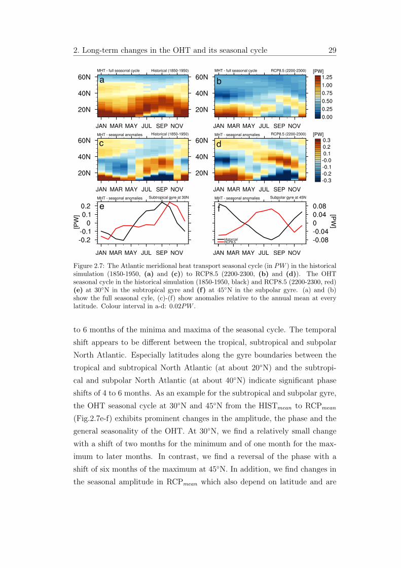
2. Long-term changes in the OHT and its seasonal cycle 29
[PW]
[PW]
[PW][P
W]
a b
fe
dc
Figure 2.7: The Atlantic meridional heat transport seasonal cycle (in PW ) in the historicalsimulation (1850-1950, (a) and (c)) to RCP8.5 (2200-2300, (b) and (d)). The OHTseasonal cycle in the historical simulation (1850-1950, black) and RCP8.5 (2200-2300, red)(e) at 30�N in the subtropical gyre and (f) at 45�N in the subpolar gyre. (a) and (b)show the full seasonal cyle, (c)-(f) show anomalies relative to the annual mean at everylatitude. Colour interval in a-d: 0.02PW .
to 6 months of the minima and maxima of the seasonal cycle. The temporal
shift appears to be di↵erent between the tropical, subtropical and subpolar
North Atlantic. Especially latitudes along the gyre boundaries between the
tropical and subtropical North Atlantic (at about 20�N) and the subtropi-
cal and subpolar North Atlantic (at about 40�N) indicate significant phase
shifts of 4 to 6 months. As an example for the subtropical and subpolar gyre,
the OHT seasonal cycle at 30�N and 45�N from the HISTmean to RCPmean
(Fig.2.7e-f) exhibits prominent changes in the amplitude, the phase and the
general seasonality of the OHT. At 30�N, we find a relatively small change
with a shift of two months for the minimum and of one month for the max-
imum to later months. In contrast, we find a reversal of the phase with a
shift of six months of the maximum at 45�N. In addition, we find changes in
the seasonal amplitude in RCPmean which also depend on latitude and are
30 2.1. The OHT seasonal cycle in a MPI-ESM climate projection
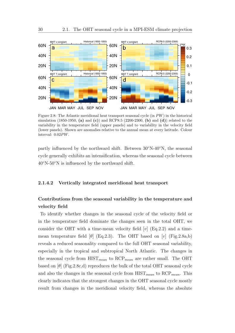
Figure 2.8: The Atlantic meridional heat transport seasonal cycle (in PW ) in the historicalsimulation (1850-1950, (a) and (c)) and RCP8.5 (2200-2300, (b) and (d)) related to thevariability in the temperature field (upper panels) and to variability in the velocity field(lower panels). Shown are anomalies relative to the annual mean at every latitude. Colourinterval: 0.02PW .
partly influenced by the northward shift. Between 30�N-40�N, the seasonal
cycle generally exhibits an intensification, whereas the seasonal cycle between
40�N-50�N is influenced by the northward shift.
2.1.4.2 Vertically integrated meridional heat transport
Contributions from the seasonal variability in the temperature and
velocity field
To identify whether changes in the seasonal cycle of the velocity field or
in the temperature field dominate the changes seen in the total OHT, we
consider the OHT with a time-mean velocity field [v] (Eq.2.2) and a time-
mean temperature field [✓] (Eq.2.3). The OHT based on [v] (Fig.2.8a,b)
reveals a reduced seasonality compared to the full OHT seasonal variability,
especially in the tropical and subtropical North Atlantic. The changes in
the seasonal cycle from HISTmean to RCPmean are rather small. The OHT
based on [✓] (Fig.2.8c,d) reproduces the bulk of the total OHT seasonal cycle
and also the changes in the seasonal cycle from HISTmean to RCPmean. This
clearly indicates that the strongest changes in the OHT seasonal cycle mostly
result from changes in the meridional velocity field, whereas the absolute
2. Long-term changes in the OHT and its seasonal cycle 31
Overturning heat transport Historical (1850-1950) Overturning heat transport RCP8.5(2200-2300)
Gyre heat transport Historical (1850-1950) Gyre heat transport RCP8.5(2200-2300)
[PW]
a b
dc
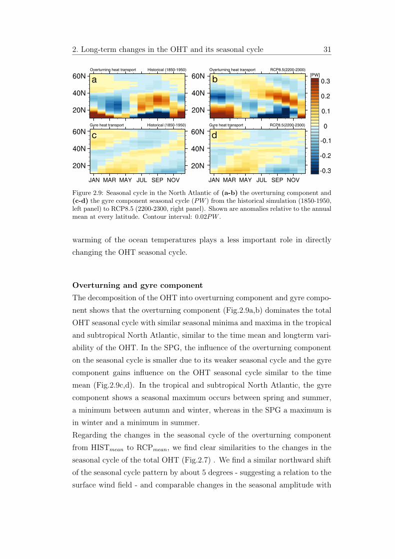
Figure 2.9: Seasonal cycle in the North Atlantic of (a-b) the overturning component and(c-d) the gyre component seasonal cycle (PW ) from the historical simulation (1850-1950,left panel) to RCP8.5 (2200-2300, right panel). Shown are anomalies relative to the annualmean at every latitude. Contour interval: 0.02PW .
warming of the ocean temperatures plays a less important role in directly
changing the OHT seasonal cycle.
Overturning and gyre component
The decomposition of the OHT into overturning component and gyre compo-
nent shows that the overturning component (Fig.2.9a,b) dominates the total
OHT seasonal cycle with similar seasonal minima and maxima in the tropical
and subtropical North Atlantic, similar to the time mean and longterm vari-
ability of the OHT. In the SPG, the influence of the overturning component
on the seasonal cycle is smaller due to its weaker seasonal cycle and the gyre
component gains influence on the OHT seasonal cycle similar to the time
mean (Fig.2.9c,d). In the tropical and subtropical North Atlantic, the gyre
component shows a seasonal maximum occurs between spring and summer,
a minimum between autumn and winter, whereas in the SPG a maximum is
in winter and a minimum in summer.
Regarding the changes in the seasonal cycle of the overturning component
from HISTmean to RCPmean, we find clear similarities to the changes in the
seasonal cycle of the total OHT (Fig.2.7) . We find a similar northward shift
of the seasonal cycle pattern by about 5 degrees - suggesting a relation to the
surface wind field - and comparable changes in the seasonal amplitude with
32 2.1. The OHT seasonal cycle in a MPI-ESM climate projection
a 2-4 months shift of the minimum and maximum in the subtropical gyre
and up to 6 months shift in the subpolar gyre. This close relation shows that
changes in the seasonal cycle of the overturning component drive the changes
in the seasonal cycle of the total OHT in both the subtropical and subpolar
gyre (Fig.2.9a,b). Similarly, the overturning component determines changes
in the seasonal amplitude of the total OHT, with a reduction in the seasonal
amplitude in the tropics, an a slight increase of the amplitude between 30�N
and 45�N.
In RCPmean (Fig.2.9c,d), the gyre component reveals a slight intensification
of the seasonal amplitude in tropical latitudes, while no significant changes
in the seasonal amplitude occur in the subtropical and subpolar gyre. Appar-
ently, important changes for the gyre component’s seasonal cycle take place
at about 40�N where the gyre boundary is situated in the model. We find a
northward shift in the seasonal cycle pattern following the northward shift in
the barotropic stream function and the zonal-mean zonal wind (Fig.2.2).
Zonal-mean zonal wind
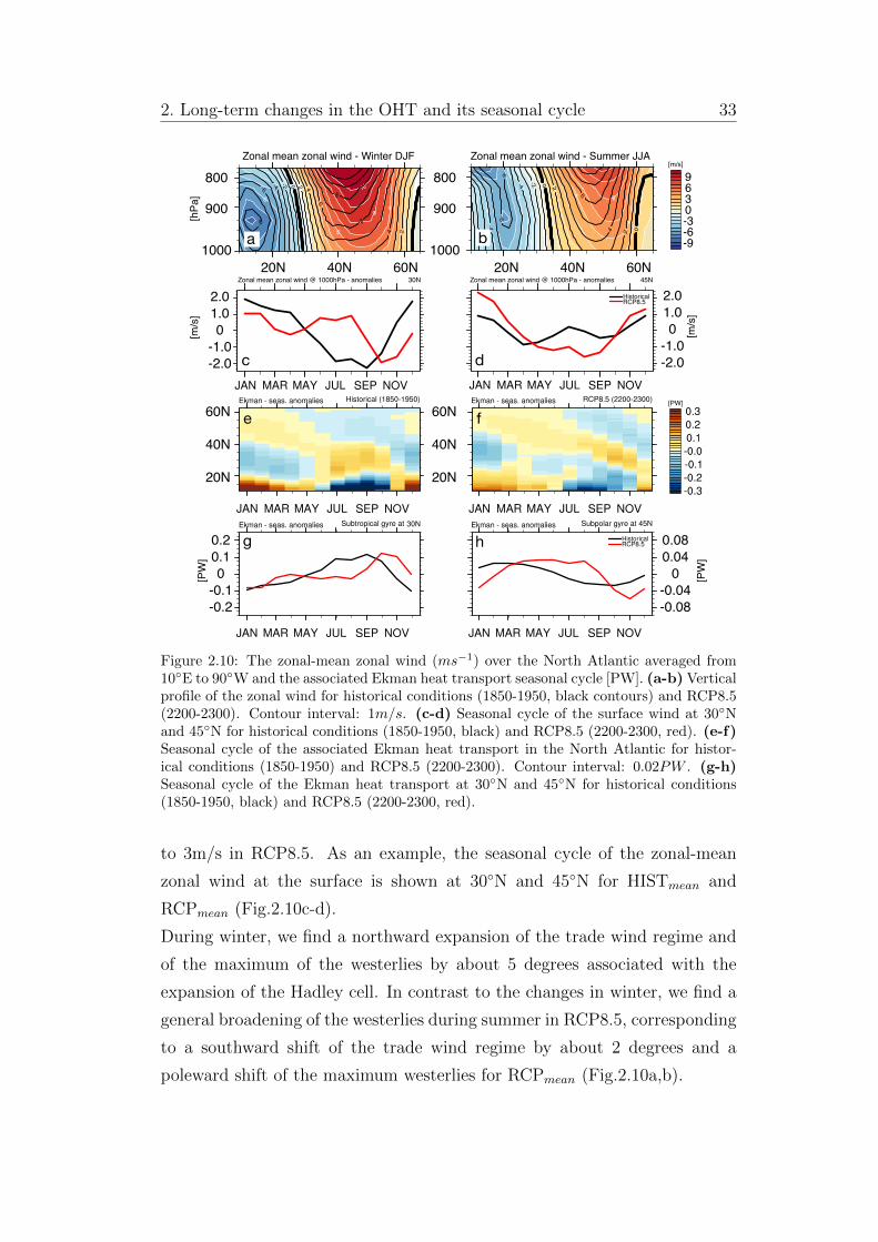
The zonal-mean zonal wind also exhibits a seasonal cycle with the seasonal
maximum of the atmospheric westerly jet in winter and meridional shifts of
the position of the jet from summer to winter in HISTmean (Fig.2.10a,b; shown
is the full zonal-mean zonal velocity field). These seasonal variations undergo
changes in amplitude and position of the jet, and temporal changes in the
seasonal cycle in RCP8.5 (c.f. Lu et al., 2014). We find an intensification of
the surface easterlies between 20�N and 30�N during winter and a reduction
of the surface westerlies between 30�N and 40�N over the subtropical North
Atlantic accompanied by an intensification of the westerlies over the subpolar
North Atlantic (40�N-60�N) from HISTmean to RCPmean. Changes of the
zonal wind during summer lead to reduced easterly winds over the subtropical
gyre, reduced westerlies between 40�N and 50�N and enhanced westerlies
north of 50�N during summer (Fig.2.10a,b). The westerlies (30�N-60�N) show
a maximum seasonal amplitude of about 3m/s at the surface, which remains
of the same amplitude in RCP8.5. The trade winds towards the equator
(south of 30�N) show a seasonal amplitude of almost 6m/s, which decreases
2. Long-term changes in the OHT and its seasonal cycle 33
0.20.10
-0.1-0.2
0.080.04
0-0.04-0.08
2.01.00
-1.0-2.0
2.01.00
-1.0-2.0
[m/s
]
[m/s
][P
W]
[PW
]
Zonal mean zonal wind @ 1000hPa - anomalies 30N Zonal mean zonal wind @ 1000hPa - anomalies 45N
60N
40N
20N
20N 40N 60N
800
900
1000
800
900
1000
9630-3-6-9
[hPa
]
Zonal mean zonal wind - Winter DJF Zonal mean zonal wind - Summer JJA[m/s]
[PW]
20N 40N 60N
60N
40N
20N
a b
c d
e f
g h
Figure 2.10: The zonal-mean zonal wind (ms�1) over the North Atlantic averaged from10�E to 90�W and the associated Ekman heat transport seasonal cycle [PW]. (a-b) Verticalprofile of the zonal wind for historical conditions (1850-1950, black contours) and RCP8.5(2200-2300). Contour interval: 1m/s. (c-d) Seasonal cycle of the surface wind at 30�Nand 45�N for historical conditions (1850-1950, black) and RCP8.5 (2200-2300, red). (e-f)Seasonal cycle of the associated Ekman heat transport in the North Atlantic for histor-ical conditions (1850-1950) and RCP8.5 (2200-2300). Contour interval: 0.02PW . (g-h)Seasonal cycle of the Ekman heat transport at 30�N and 45�N for historical conditions(1850-1950, black) and RCP8.5 (2200-2300, red).
to 3m/s in RCP8.5. As an example, the seasonal cycle of the zonal-mean
zonal wind at the surface is shown at 30�N and 45�N for HISTmean and
RCPmean (Fig.2.10c-d).
During winter, we find a northward expansion of the trade wind regime and
of the maximum of the westerlies by about 5 degrees associated with the
expansion of the Hadley cell. In contrast to the changes in winter, we find a
general broadening of the westerlies during summer in RCP8.5, corresponding
to a southward shift of the trade wind regime by about 2 degrees and a
poleward shift of the maximum westerlies for RCPmean (Fig.2.10a,b).
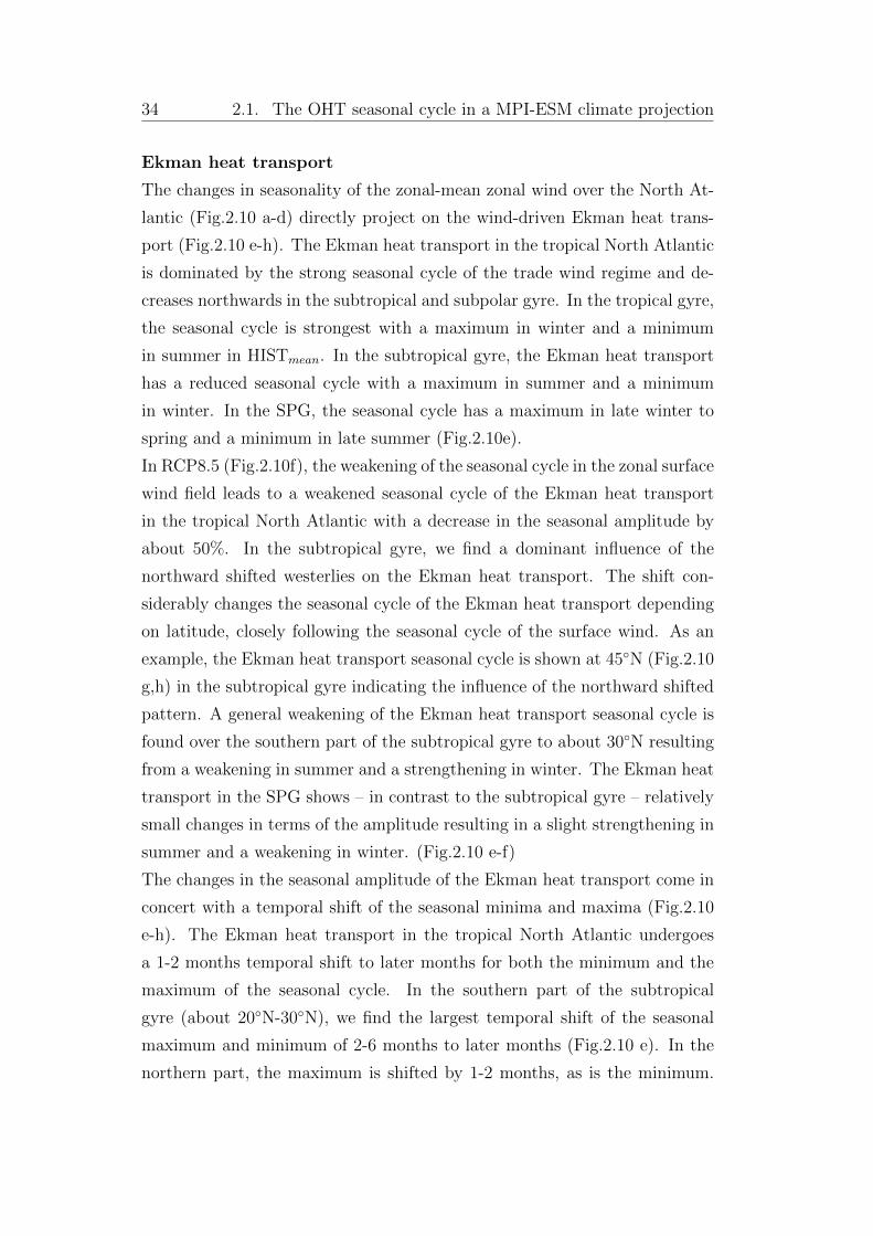
34 2.1. The OHT seasonal cycle in a MPI-ESM climate projection
Ekman heat transport
The changes in seasonality of the zonal-mean zonal wind over the North At-
lantic (Fig.2.10 a-d) directly project on the wind-driven Ekman heat trans-
port (Fig.2.10 e-h). The Ekman heat transport in the tropical North Atlantic
is dominated by the strong seasonal cycle of the trade wind regime and de-
creases northwards in the subtropical and subpolar gyre. In the tropical gyre,
the seasonal cycle is strongest with a maximum in winter and a minimum
in summer in HISTmean. In the subtropical gyre, the Ekman heat transport
has a reduced seasonal cycle with a maximum in summer and a minimum
in winter. In the SPG, the seasonal cycle has a maximum in late winter to
spring and a minimum in late summer (Fig.2.10e).
In RCP8.5 (Fig.2.10f), the weakening of the seasonal cycle in the zonal surface
wind field leads to a weakened seasonal cycle of the Ekman heat transport
in the tropical North Atlantic with a decrease in the seasonal amplitude by
about 50%. In the subtropical gyre, we find a dominant influence of the
northward shifted westerlies on the Ekman heat transport. The shift con-
siderably changes the seasonal cycle of the Ekman heat transport depending
on latitude, closely following the seasonal cycle of the surface wind. As an
example, the Ekman heat transport seasonal cycle is shown at 45�N (Fig.2.10
g,h) in the subtropical gyre indicating the influence of the northward shifted
pattern. A general weakening of the Ekman heat transport seasonal cycle is
found over the southern part of the subtropical gyre to about 30�N resulting
from a weakening in summer and a strengthening in winter. The Ekman heat
transport in the SPG shows – in contrast to the subtropical gyre – relatively
small changes in terms of the amplitude resulting in a slight strengthening in
summer and a weakening in winter. (Fig.2.10 e-f)
The changes in the seasonal amplitude of the Ekman heat transport come in
concert with a temporal shift of the seasonal minima and maxima (Fig.2.10
e-h). The Ekman heat transport in the tropical North Atlantic undergoes
a 1-2 months temporal shift to later months for both the minimum and the
maximum of the seasonal cycle. In the southern part of the subtropical
gyre (about 20�N-30�N), we find the largest temporal shift of the seasonal
maximum and minimum of 2-6 months to later months (Fig.2.10 e). In the
northern part, the maximum is shifted by 1-2 months, as is the minimum.
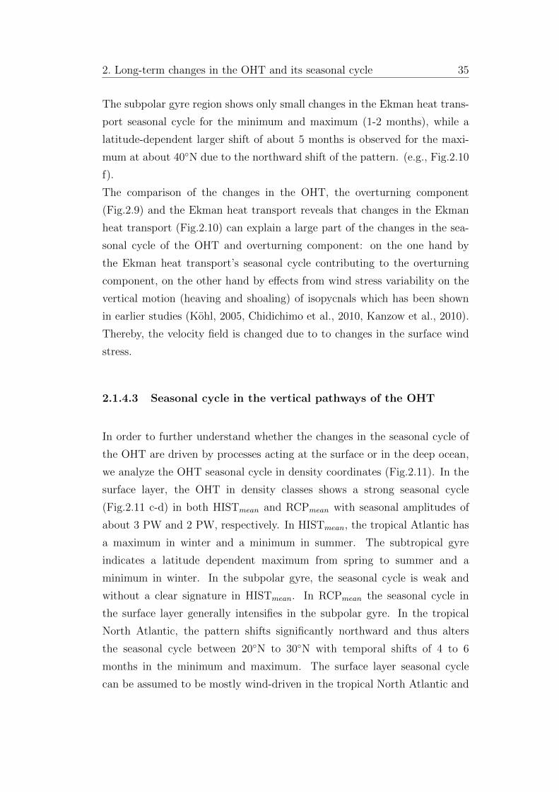
2. Long-term changes in the OHT and its seasonal cycle 35
The subpolar gyre region shows only small changes in the Ekman heat trans-
port seasonal cycle for the minimum and maximum (1-2 months), while a
latitude-dependent larger shift of about 5 months is observed for the maxi-
mum at about 40�N due to the northward shift of the pattern. (e.g., Fig.2.10
f).
The comparison of the changes in the OHT, the overturning component
(Fig.2.9) and the Ekman heat transport reveals that changes in the Ekman
heat transport (Fig.2.10) can explain a large part of the changes in the sea-
sonal cycle of the OHT and overturning component: on the one hand by
the Ekman heat transport’s seasonal cycle contributing to the overturning
component, on the other hand by e↵ects from wind stress variability on the
vertical motion (heaving and shoaling) of isopycnals which has been shown
in earlier studies (Kohl, 2005, Chidichimo et al., 2010, Kanzow et al., 2010).
Thereby, the velocity field is changed due to to changes in the surface wind
stress.
2.1.4.3 Seasonal cycle in the vertical pathways of the OHT
In order to further understand whether the changes in the seasonal cycle of
the OHT are driven by processes acting at the surface or in the deep ocean,
we analyze the OHT seasonal cycle in density coordinates (Fig.2.11). In the
surface layer, the OHT in density classes shows a strong seasonal cycle
(Fig.2.11 c-d) in both HISTmean and RCPmean with seasonal amplitudes of
about 3 PW and 2 PW, respectively. In HISTmean, the tropical Atlantic has
a maximum in winter and a minimum in summer. The subtropical gyre
indicates a latitude dependent maximum from spring to summer and a
minimum in winter. In the subpolar gyre, the seasonal cycle is weak and
without a clear signature in HISTmean. In RCPmean the seasonal cycle in
the surface layer generally intensifies in the subpolar gyre. In the tropical
North Atlantic, the pattern shifts significantly northward and thus alters
the seasonal cycle between 20�N to 30�N with temporal shifts of 4 to 6
months in the minimum and maximum. The surface layer seasonal cycle
can be assumed to be mostly wind-driven in the tropical North Atlantic and
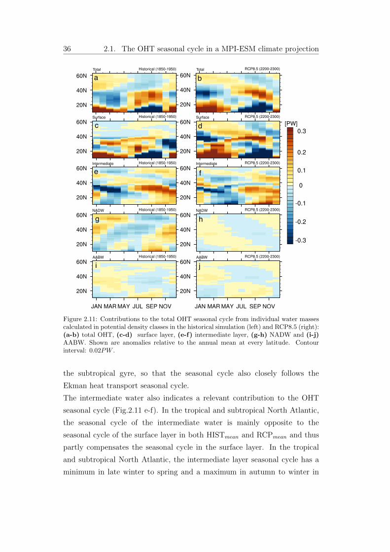
36 2.1. The OHT seasonal cycle in a MPI-ESM climate projection
[PW]
hg
e f
dc
TotalTotal
a b
ji
Figure 2.11: Contributions to the total OHT seasonal cycle from individual water massescalculated in potential density classes in the historical simulation (left) and RCP8.5 (right):(a-b) total OHT, (c-d) surface layer, (e-f) intermediate layer, (g-h) NADW and (i-j)AABW. Shown are anomalies relative to the annual mean at every latitude. Contourinterval: 0.02PW .
the subtropical gyre, so that the seasonal cycle also closely follows the
Ekman heat transport seasonal cycle.
The intermediate water also indicates a relevant contribution to the OHT
seasonal cycle (Fig.2.11 e-f). In the tropical and subtropical North Atlantic,
the seasonal cycle of the intermediate water is mainly opposite to the
seasonal cycle of the surface layer in both HISTmean and RCPmean and thus
partly compensates the seasonal cycle in the surface layer. In the tropical
and subtropical North Atlantic, the intermediate layer seasonal cycle has a
minimum in late winter to spring and a maximum in autumn to winter in
2. Long-term changes in the OHT and its seasonal cycle 37
HISTmean, as well as a minimum in winter to spring and a maximum in
autumn to winter in RCPmean. From HISTmean to RCPmean, the pattern
shows shifts in the seasonal cycle of about 1 month to later months, but
no clear northward shift as in the surface layer. The seasonal cycle in
the subpolar gyre indicates general phase shift of up to 6 months from
HISTmean to RCPmean with a shift of the maximum from summer to winter
between approximately 40�N to 50�N and a shift of the maximum from
winter to spring between 50�N and 60�N.
In the NADW (Fig.2.11 g-h), significant changes occur resulting from
changes in the water mass formation in the North Atlantic. In the
HISTmean, the formation of NADW is present and leads to a seasonal cycle
in the OHT of the NADW giving an important contribution especially in
the subpolar gyre. In the subpolar gyre, the NADW shows a maximum in
winter to spring and a minimum in summer to autumn. In the subtropical
gyre, the NADW seasonal maximum is in winter, the minimum in spring to
summer. In RCPmean the seasonal cycle is almost not existent in the
remaining OHT of the NADW with a decrease of the seasonal amplitude
from about 0.2 PW to almost 0 PW, thus showing a surface-ward shift of
the processes acting on the OHT seasonal cycle.
The AABW seasonal cycle is generally weak and thus does not significantly
contribute to the full OHT seasonal cycle (Fig.2.11 i-j). Still, we find a
seasonal cycle in HISTmean with a maximum in summer and a minimum
in winter in the tropical North Atlantic, and a maximum in winter and
a minimum in late summer in the subtropical and subpolar gyre. For
RCPmean we find changes in the seasonal cycle with a northward shift of the
pattern and also latitude dependent temporal shifts. These changes in the
AABW might result from changed dynamics in the Southern Ocean also
influencing the global ocean circulation, which we do not focus on in this
study and thus need further analysis.
38 2.1. The OHT seasonal cycle in a MPI-ESM climate projection
2.1.5 Discussion
The changes in the Atlantic meridional heat transport in future climate pro-
jections in MPI-ESM are accompanied by changes in the seasonal cycle of the
oceanic OHT. Based on the scenario RCP8.5, we have identified changes in
the mean climate state of the North Atlantic and in the associated seasonal
cycle of the OHT.
We find a weakening of the mean OHT by 30-50% associated with a weak-
ening of the overturning heat transport in RCP8.5. The weakening of the
mean OHT comes in concert with the weakening of the AMOC’s geostrophic
transport by the end of the 23rd century in MPI-ESM indicating a direct rela-
tion between OHT and AMOC’s strength. This direct relation has also been
found from observations and model studies based on the RAPID array in the
North Atlantic (e.g. Johns et al., 2011, Msadek et al., 2013). Recent CMIP5
experiments show an overall reduction of the AMOC in the multi-model en-
semble by about 40% for RCP8.5 by the end of the 23rd century (Weaver
et al., 2012, Cheng et al., 2013), which can be attributed to a reduction of
deep water formation in the North Atlantic, especially in the Labrador Sea
and Greenland Sea (Vellinga and Wood, 2002). As shown for the AMOC in
density coordinates, the deep overturning cell which is fed by the NADW is
strongly weakened in RCP8.5 in accordance with the absence of deep water
formation in the Nordic seas and the Labrador Sea.
The general AMOC weakening found in most models of the CMIP5 multi-
model ensemble gives reason to expect that a similar weakening of the OHT
as found in MPI-ESM might be found in other CMIP5 models. As shown
by Drijfhout et al. (2012), various CMIP5 models show the prominent area
of reduced warming (“warming hole”) in the subpolar North Atlantic surface
temperatures for longterm changes, which can already be seen in the histor-
ical simulations as well as in recent observations from the Goddard Institute
for Space Studies surface temperature analysis dataset (Hansen et al., 2010).
This signal might be related to an adjustment of the gyre circulation already
taking place in the present climate state that preconditions a decline of the
AMOC and of the associated OHT, as well as possible changes in the seasonal
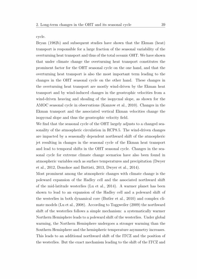
2. Long-term changes in the OHT and its seasonal cycle 39
cycle.
Bryan (1982b) and subsequent studies have shown that the Ekman (heat)
transport is responsible for a large fraction of the seasonal variability of the
overturning heat transport and thus of the total oceanic OHT. We have shown
that under climate change the overturning heat transport constitutes the
prominent factor for the OHT seasonal cycle on the one hand, and that the
overturning heat transport is also the most important term leading to the
changes in the OHT seasonal cycle on the other hand. These changes in
the overturning heat transport are mostly wind-driven by the Ekman heat
transport and by wind-induced changes in the geostrophic velocities from a
wind-driven heaving and shoaling of the isopycnal slope, as shown for the
AMOC seasonal cycle in observations (Kanzow et al., 2010). Changes in the
Ekman transport and the associated vertical Ekman velocities change the
isopycnal slope and thus the geostrophic velocity field.
We find that the seasonal cycle of the OHT largely adjusts to a changed sea-
sonality of the atmospheric circulation in RCP8.5. The wind-driven changes
are impacted by a seasonally dependent northward shift of the atmospheric
jet resulting in changes in the seasonal cycle of the Ekman heat transport
and lead to temporal shifts in the OHT seasonal cycle. Changes in the sea-
sonal cycle for extreme climate change scenarios have also been found in
atmospheric variables such as surface temperatures and precipitation (Dwyer
et al., 2012, Donohoe and Battisti, 2013, Dwyer et al., 2014).
Most prominent among the atmospheric changes with climate change is the
poleward expansion of the Hadley cell and the associated northward shift
of the mid-latitude westerlies (Lu et al., 2014). A warmer planet has been
shown to lead to an expansion of the Hadley cell and a poleward shift of
the westerlies in both dynamical core (Butler et al., 2010) and complex cli-
mate models (Lu et al., 2008). According to Toggweiler (2009) the northward
shift of the westerlies follows a simple mechanism: a systematically warmer
Northern Hemisphere leads to a poleward shift of the westerlies. Under global
warming, the Northern Hemisphere undergoes a stronger warming than the
Southern Hemisphere and the hemispheric temperature asymmetry increases.
This leads to an additional northward shift of the ITCZ and the position of
the westerlies. But the exact mechanism leading to the shift of the ITCZ and
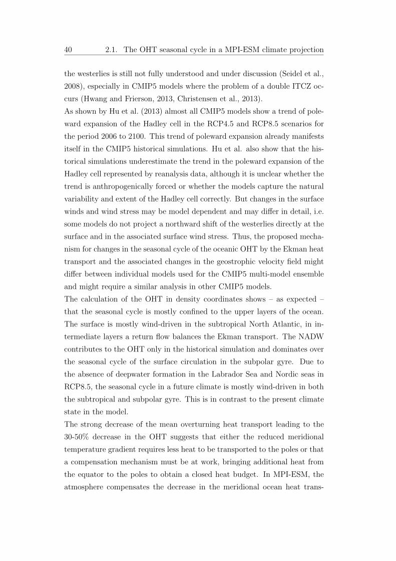
40 2.1. The OHT seasonal cycle in a MPI-ESM climate projection
the westerlies is still not fully understood and under discussion (Seidel et al.,
2008), especially in CMIP5 models where the problem of a double ITCZ oc-
curs (Hwang and Frierson, 2013, Christensen et al., 2013).
As shown by Hu et al. (2013) almost all CMIP5 models show a trend of pole-
ward expansion of the Hadley cell in the RCP4.5 and RCP8.5 scenarios for
the period 2006 to 2100. This trend of poleward expansion already manifests
itself in the CMIP5 historical simulations. Hu et al. also show that the his-
torical simulations underestimate the trend in the poleward expansion of the
Hadley cell represented by reanalysis data, although it is unclear whether the
trend is anthropogenically forced or whether the models capture the natural
variability and extent of the Hadley cell correctly. But changes in the surface
winds and wind stress may be model dependent and may di↵er in detail, i.e.
some models do not project a northward shift of the westerlies directly at the
surface and in the associated surface wind stress. Thus, the proposed mecha-
nism for changes in the seasonal cycle of the oceanic OHT by the Ekman heat
transport and the associated changes in the geostrophic velocity field might
di↵er between individual models used for the CMIP5 multi-model ensemble
and might require a similar analysis in other CMIP5 models.
The calculation of the OHT in density coordinates shows – as expected –
that the seasonal cycle is mostly confined to the upper layers of the ocean.
The surface is mostly wind-driven in the subtropical North Atlantic, in in-
termediate layers a return flow balances the Ekman transport. The NADW
contributes to the OHT only in the historical simulation and dominates over
the seasonal cycle of the surface circulation in the subpolar gyre. Due to
the absence of deepwater formation in the Labrador Sea and Nordic seas in
RCP8.5, the seasonal cycle in a future climate is mostly wind-driven in both
the subtropical and subpolar gyre. This is in contrast to the present climate
state in the model.
The strong decrease of the mean overturning heat transport leading to the
30-50% decrease in the OHT suggests that either the reduced meridional
temperature gradient requires less heat to be transported to the poles or that
a compensation mechanism must be at work, bringing additional heat from
the equator to the poles to obtain a closed heat budget. In MPI-ESM, the
atmosphere compensates the decrease in the meridional ocean heat trans-
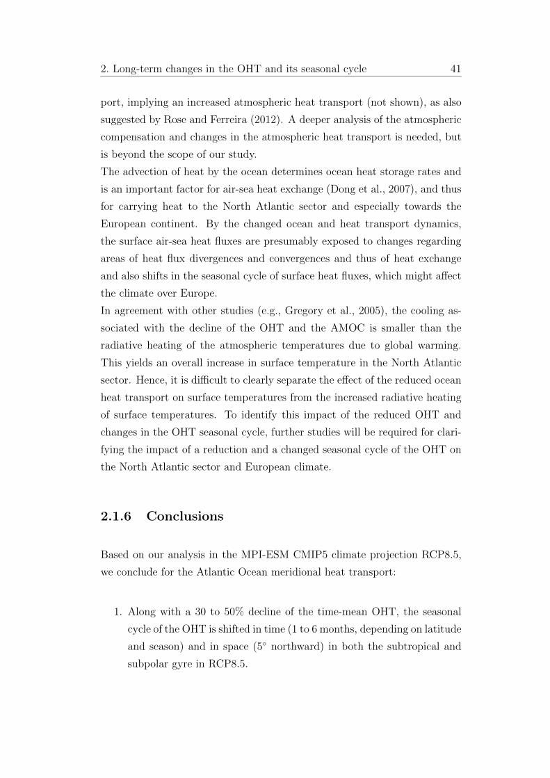
2. Long-term changes in the OHT and its seasonal cycle 41
port, implying an increased atmospheric heat transport (not shown), as also
suggested by Rose and Ferreira (2012). A deeper analysis of the atmospheric
compensation and changes in the atmospheric heat transport is needed, but
is beyond the scope of our study.
The advection of heat by the ocean determines ocean heat storage rates and
is an important factor for air-sea heat exchange (Dong et al., 2007), and thus
for carrying heat to the North Atlantic sector and especially towards the
European continent. By the changed ocean and heat transport dynamics,
the surface air-sea heat fluxes are presumably exposed to changes regarding
areas of heat flux divergences and convergences and thus of heat exchange
and also shifts in the seasonal cycle of surface heat fluxes, which might a↵ect
the climate over Europe.
In agreement with other studies (e.g., Gregory et al., 2005), the cooling as-
sociated with the decline of the OHT and the AMOC is smaller than the
radiative heating of the atmospheric temperatures due to global warming.
This yields an overall increase in surface temperature in the North Atlantic
sector. Hence, it is di�cult to clearly separate the e↵ect of the reduced ocean
heat transport on surface temperatures from the increased radiative heating
of surface temperatures. To identify this impact of the reduced OHT and
changes in the OHT seasonal cycle, further studies will be required for clari-
fying the impact of a reduction and a changed seasonal cycle of the OHT on
the North Atlantic sector and European climate.
2.1.6 Conclusions
Based on our analysis in the MPI-ESM CMIP5 climate projection RCP8.5,
we conclude for the Atlantic Ocean meridional heat transport:
1. Along with a 30 to 50% decline of the time-mean OHT, the seasonal
cycle of the OHT is shifted in time (1 to 6 months, depending on latitude
and season) and in space (5� northward) in both the subtropical and
subpolar gyre in RCP8.5.
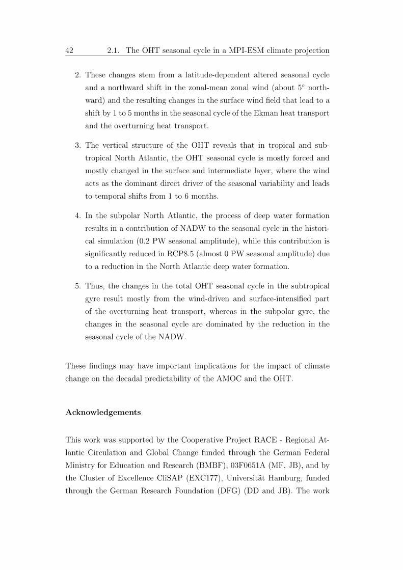
42 2.1. The OHT seasonal cycle in a MPI-ESM climate projection
2. These changes stem from a latitude-dependent altered seasonal cycle
and a northward shift in the zonal-mean zonal wind (about 5� north-
ward) and the resulting changes in the surface wind field that lead to a
shift by 1 to 5 months in the seasonal cycle of the Ekman heat transport
and the overturning heat transport.
3. The vertical structure of the OHT reveals that in tropical and sub-
tropical North Atlantic, the OHT seasonal cycle is mostly forced and
mostly changed in the surface and intermediate layer, where the wind
acts as the dominant direct driver of the seasonal variability and leads
to temporal shifts from 1 to 6 months.
4. In the subpolar North Atlantic, the process of deep water formation
results in a contribution of NADW to the seasonal cycle in the histori-
cal simulation (0.2 PW seasonal amplitude), while this contribution is
significantly reduced in RCP8.5 (almost 0 PW seasonal amplitude) due
to a reduction in the North Atlantic deep water formation.
5. Thus, the changes in the total OHT seasonal cycle in the subtropical
gyre result mostly from the wind-driven and surface-intensified part
of the overturning heat transport, whereas in the subpolar gyre, the
changes in the seasonal cycle are dominated by the reduction in the
seasonal cycle of the NADW.
These findings may have important implications for the impact of climate
change on the decadal predictability of the AMOC and the OHT.
Acknowledgements
This work was supported by the Cooperative Project RACE - Regional At-
lantic Circulation and Global Change funded through the German Federal
Ministry for Education and Research (BMBF), 03F0651A (MF, JB), and by
the Cluster of Excellence CliSAP (EXC177), Universitat Hamburg, funded
through the German Research Foundation (DFG) (DD and JB). The work

2. Long-term changes in the OHT and its seasonal cycle 43
of WM was supported by the German Federal Ministry for Education and
Research (BMBF) project MiKlip (PT01LP1144A). Further, research lead-
ing to these results has received funding from the European Unions Seventh
Framework Programme (FP7/2007-2013) under grant agreement no. 308378
ENV.2012.6.1-1: Seasonal-to-decadal climate predictions towards climate ser-
vices [http://www.specs-fp7.eu/]. The climate simulations were performed at
the German Climate Computing Centre (DKRZ). We thank Ralf Hand for
stimulating discussions and the three anonymous reviewers for their construc-
tive comments on an earlier version of the manuscript.

44 2.1. The OHT seasonal cycle in a MPI-ESM climate projection
2. Long-term changes in the OHT and its seasonal cycle 45
2.2 The seasonal cycle of the Atlantic merid-
ional heat transport in potential temper-
ature coordinates
2.2.1 Introduction
The Atlantic meridional heat transport (OHT) is traditionally considered as
the full zonal and vertical (top to bottom) integral of the meridional tem-
perature flux which ensures a zero net mass flux across a latitude (Bryan,
1962, 1982a, Bryden and Imawaki, 2001, Siedler et al., 2013). The contri-
bution of the vertical meridional overturning circulation, the horizontal gyre
circulation and the oceanic eddy field is usually described by a decomposition
of the OHT in overturning and gyre heat transport (c.f section 2.1, Eq.2.4).
But, the vertical integration of the OHT prevents to understand the vertical
structure of the OHT and the relative contributions to the total OHT from
individual layers and circulation cells of the meridional overturning circula-
tion.
Recently, various approaches based on either observations or model experi-
ments have shown contributions of individual water masses and layers to the
total OHT (Talley, 2003, Boccaletti et al., 2005, Ferrari and Ferreira, 2011).
The analysis of Talley (2003), based on observations in the North Atlantic,
considered layers of di↵erent densities representing the water masses in the
Atlantic. She found that 60% of the mean OHT at 24�N in the North Atlantic
results from the intermediate and deep overturning, while the remaining 40%
are carried northward in a shallow overturning layer, in contrast to the tradi-
tional view, where about 90% of the heat transport are ascribed to the deep
overturning circulation at 25�N (e.g. Bryden and Imawaki, 2001).
Boccaletti et al. (2005) and Ferrari and Ferreira (2011) analyzed the vertical
structure of the heat transport based on a heat function in depth and temper-
ature coordinates. Boccaletti et al. (2005) used numerical model experiments
to calculate a heat function in cartesian (depth) coordinates. By the choice
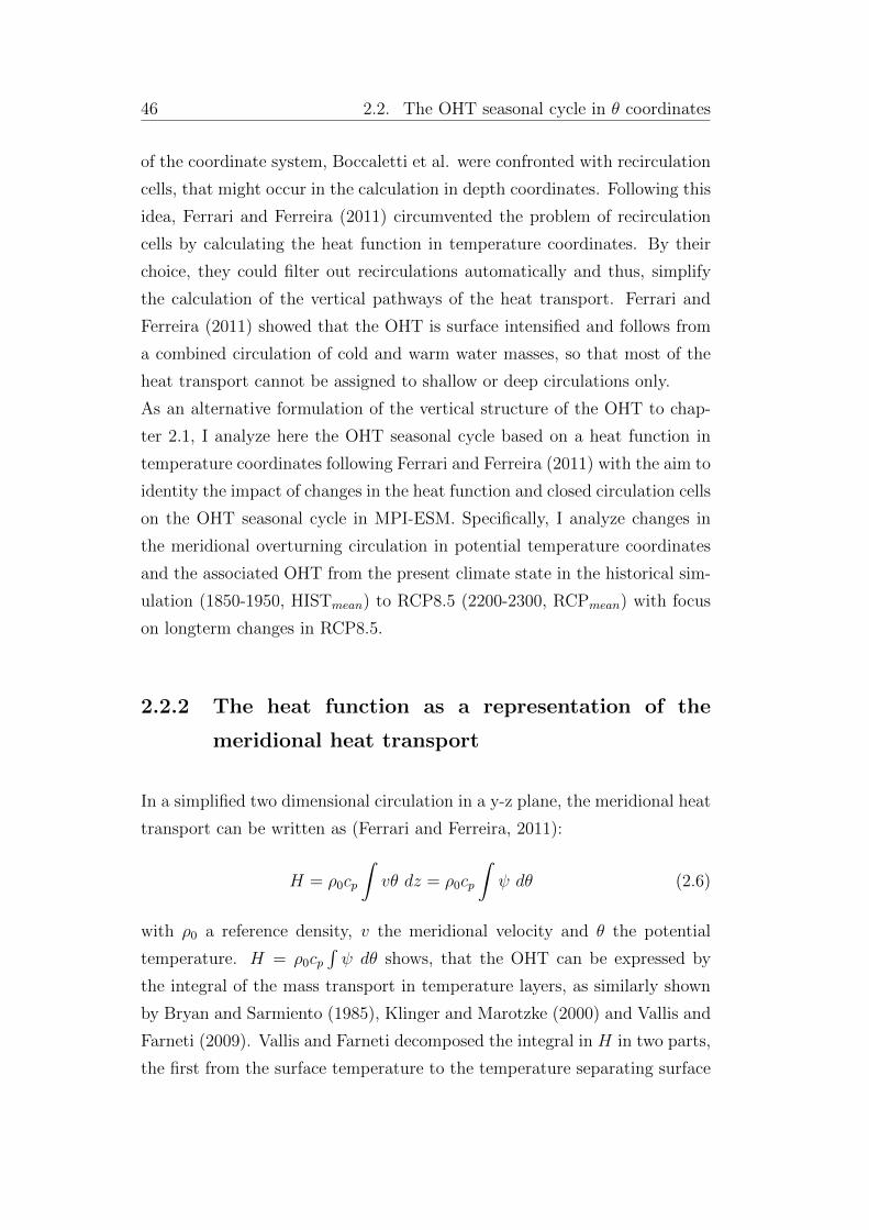
46 2.2. The OHT seasonal cycle in ✓ coordinates
of the coordinate system, Boccaletti et al. were confronted with recirculation
cells, that might occur in the calculation in depth coordinates. Following this
idea, Ferrari and Ferreira (2011) circumvented the problem of recirculation
cells by calculating the heat function in temperature coordinates. By their
choice, they could filter out recirculations automatically and thus, simplify
the calculation of the vertical pathways of the heat transport. Ferrari and
Ferreira (2011) showed that the OHT is surface intensified and follows from
a combined circulation of cold and warm water masses, so that most of the
heat transport cannot be assigned to shallow or deep circulations only.
As an alternative formulation of the vertical structure of the OHT to chap-
ter 2.1, I analyze here the OHT seasonal cycle based on a heat function in
temperature coordinates following Ferrari and Ferreira (2011) with the aim to
identity the impact of changes in the heat function and closed circulation cells
on the OHT seasonal cycle in MPI-ESM. Specifically, I analyze changes in
the meridional overturning circulation in potential temperature coordinates
and the associated OHT from the present climate state in the historical sim-
ulation (1850-1950, HISTmean) to RCP8.5 (2200-2300, RCPmean) with focus
on longterm changes in RCP8.5.
2.2.2 The heat function as a representation of the
meridional heat transport
In a simplified two dimensional circulation in a y-z plane, the meridional heat
transport can be written as (Ferrari and Ferreira, 2011):
H = ⇢0
cp
Zv✓ dz = ⇢
0
cp
Z d✓ (2.6)
with ⇢0
a reference density, v the meridional velocity and ✓ the potential
temperature. H = ⇢0
cpR d✓ shows, that the OHT can be expressed by
the integral of the mass transport in temperature layers, as similarly shown
by Bryan and Sarmiento (1985), Klinger and Marotzke (2000) and Vallis and
Farneti (2009). Vallis and Farneti decomposed the integral in H in two parts,
the first from the surface temperature to the temperature separating surface
2. Long-term changes in the OHT and its seasonal cycle 47
and deep circulations, the second over the remaining cold temperatures.
Ferrari and Ferreira (2011) extended the approach to involve overlapping
circulations in same temperature classes, what they call mixed overturning
circulations. By their definition, the heat function in potential temperature
coordinates can be derived from the stream function of the zonally averaged
mass flux in temperature coordinates as follows:
(y, ✓) =
Z Z
✓0✓
vdxdz. (2.7)
The overbar denotes a long-time average of the stream function at latitude y
and temperature ✓. It can be shown, that this stream function describes the
residual overturning streamfunction (Andrews, 1983) in ✓ coordinates, and
thus involves contributions from both, the mean flow and from the bolus flow
from the eddy field (deviations from the zonal and temporal mean; Nurser
and Lee, 2004).
A heat function H in steady state can then be defined as
H(y, ✓) ⌘✓Z
✓B
⇢0
cp (y, ✓) d✓, (2.8)
where is the mass stream function. A more detailed derivation of H is
given in Ferrari and Ferreira (2011).
To identify now individual pathways of the OHT in the overturning circu-
lation, we consider a combination of the heat function and the overturning
stream function. Based on the overturning stream function, we define closed
overturning circulation cells for the OHT for temperature ranges between ✓u
and ✓l
OHT (y, ✓u, ✓l) =
Z ✓u
✓l
⇢0
cp( (y, ✓)� (y, ✓l)) d✓. (2.9)
For circulations enclosed from other flows, the surrounding flow
⇢0
cp (y, ✓l)(✓u � ✓l) must be subtracted:
OHT (y, ✓u, ✓l) = H(y, ✓u)�H(y, ✓l)� ⇢0
cp (y, ✓l)(✓u � ✓l) (2.10)
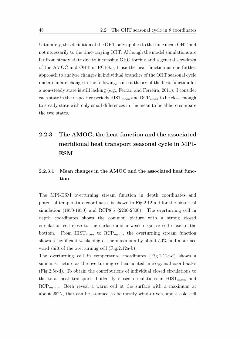
48 2.2. The OHT seasonal cycle in ✓ coordinates
Ultimately, this definition of the OHT only applies to the time mean OHT and
not necessarily to the time-varying OHT. Although the model simulations are
far from steady state due to increasing GHG forcing and a general slowdown
of the AMOC and OHT in RCP8.5, I use the heat function as one further
approach to analyze changes in individual branches of the OHT seasonal cycle
under climate change in the following, since a theory of the heat function for
a non-steady state is still lacking (e.g., Ferrari and Ferreira, 2011). I consider
each state in the respective periods HISTmean and RCPmean to be close enough
to steady state with only small di↵erences in the mean to be able to compare
the two states.
2.2.3 The AMOC, the heat function and the associated
meridional heat transport seasonal cycle in MPI-
ESM
2.2.3.1 Mean changes in the AMOC and the associated heat func-
tion
The MPI-ESM overturning stream function in depth coordinates and
potential temperature coordinates is shown in Fig.2.12 a-d for the historical
simulation (1850-1950) and RCP8.5 (2200-2300). The overturning cell in
depth coordinates shows the common picture with a strong closed
circulation cell close to the surface and a weak negative cell close to the
bottom. From HISTmean to RCPmean, the overturning stream function
shows a significant weakening of the maximum by about 50% and a surface
ward shift of the overturning cell (Fig.2.12a-b).
The overturning cell in temperature coordinates (Fig.2.12c-d) shows a
similar structure as the overturning cell calculated in isopycnal coordinates
(Fig.2.5c-d). To obtain the contributions of individual closed circulations to
the total heat transport, I identify closed circulations in HISTmean and
RCPmean. Both reveal a warm cell at the surface with a maximum at
about 25�N, that can be assumed to be mostly wind-driven, and a cold cell
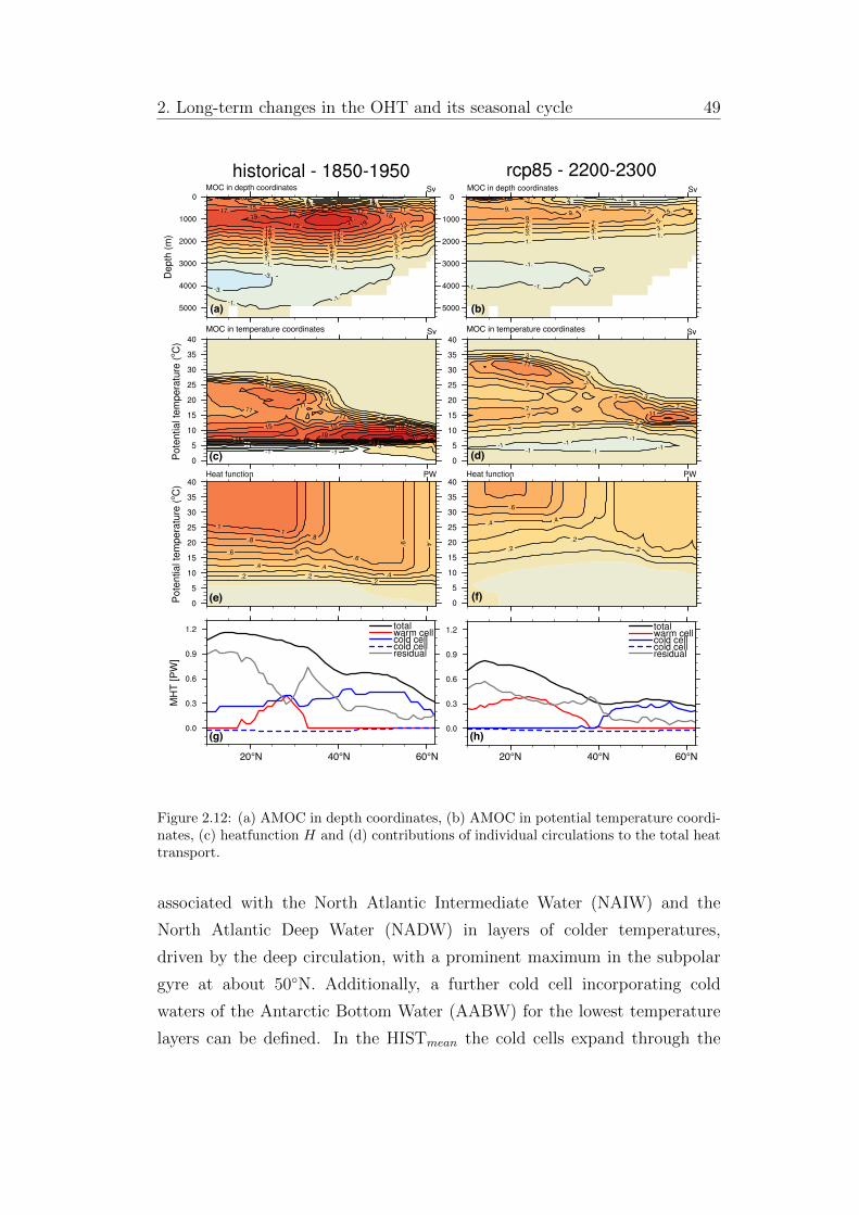
2. Long-term changes in the OHT and its seasonal cycle 49
20°N 60°N40°N 20°N 60°N40°N
(a) (b)
(c) (d)
(e) (f)
(g) (h)
MOC in temperature coordinates MOC in temperature coordinates
Figure 2.12: (a) AMOC in depth coordinates, (b) AMOC in potential temperature coordi-nates, (c) heatfunction H and (d) contributions of individual circulations to the total heattransport.
associated with the North Atlantic Intermediate Water (NAIW) and the
North Atlantic Deep Water (NADW) in layers of colder temperatures,
driven by the deep circulation, with a prominent maximum in the subpolar
gyre at about 50�N. Additionally, a further cold cell incorporating cold
waters of the Antarctic Bottom Water (AABW) for the lowest temperature
layers can be defined. In the HISTmean the cold cells expand through the
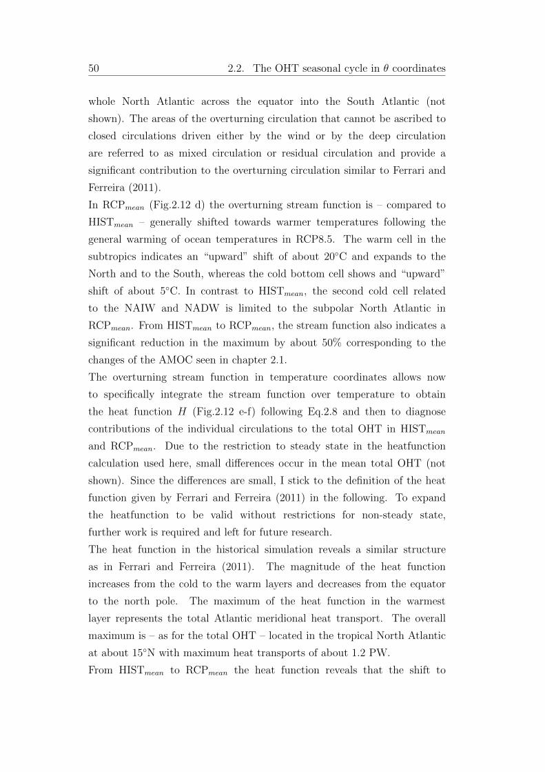
50 2.2. The OHT seasonal cycle in ✓ coordinates
whole North Atlantic across the equator into the South Atlantic (not
shown). The areas of the overturning circulation that cannot be ascribed to
closed circulations driven either by the wind or by the deep circulation
are referred to as mixed circulation or residual circulation and provide a
significant contribution to the overturning circulation similar to Ferrari and
Ferreira (2011).
In RCPmean (Fig.2.12 d) the overturning stream function is – compared to
HISTmean – generally shifted towards warmer temperatures following the
general warming of ocean temperatures in RCP8.5. The warm cell in the
subtropics indicates an “upward” shift of about 20�C and expands to the
North and to the South, whereas the cold bottom cell shows and “upward”
shift of about 5�C. In contrast to HISTmean, the second cold cell related
to the NAIW and NADW is limited to the subpolar North Atlantic in
RCPmean. From HISTmean to RCPmean, the stream function also indicates a
significant reduction in the maximum by about 50% corresponding to the
changes of the AMOC seen in chapter 2.1.
The overturning stream function in temperature coordinates allows now
to specifically integrate the stream function over temperature to obtain
the heat function H (Fig.2.12 e-f) following Eq.2.8 and then to diagnose
contributions of the individual circulations to the total OHT in HISTmean
and RCPmean. Due to the restriction to steady state in the heatfunction
calculation used here, small di↵erences occur in the mean total OHT (not
shown). Since the di↵erences are small, I stick to the definition of the heat
function given by Ferrari and Ferreira (2011) in the following. To expand
the heatfunction to be valid without restrictions for non-steady state,
further work is required and left for future research.
The heat function in the historical simulation reveals a similar structure
as in Ferrari and Ferreira (2011). The magnitude of the heat function
increases from the cold to the warm layers and decreases from the equator
to the north pole. The maximum of the heat function in the warmest
layer represents the total Atlantic meridional heat transport. The overall
maximum is – as for the total OHT – located in the tropical North Atlantic
at about 15�N with maximum heat transports of about 1.2 PW.
From HISTmean to RCPmean the heat function reveals that the shift to
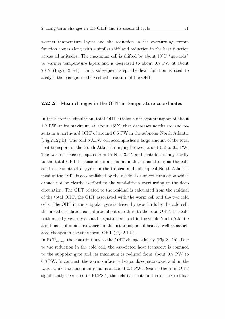
2. Long-term changes in the OHT and its seasonal cycle 51
warmer temperature layers and the reduction in the overturning stream
function comes along with a similar shift and reduction in the heat function
across all latitudes. The maximum cell is shifted by about 10�C “upwards”
to warmer temperature layers and is decreased to about 0.7 PW at about
20�N (Fig.2.12 e-f). In a subsequent step, the heat function is used to
analyze the changes in the vertical structure of the OHT.
2.2.3.2 Mean changes in the OHT in temperature coordinates
In the historical simulation, total OHT attains a net heat transport of about
1.2 PW at its maximum at about 15�N, that decreases northward and re-
sults in a northward OHT of around 0.6 PW in the subpolar North Atlantic
(Fig.2.12g-h). The cold NADW cell accomplishes a large amount of the total
heat transport in the North Atlantic ranging between about 0.2 to 0.5 PW.
The warm surface cell spans from 15�N to 35�N and contributes only locally
to the total OHT because of its a maximum that is as strong as the cold
cell in the subtropical gyre. In the tropical and subtropical North Atlantic,
most of the OHT is accomplished by the residual or mixed circulation which
cannot not be clearly ascribed to the wind-driven overturning or the deep
circulation. The OHT related to the residual is calculated from the residual
of the total OHT, the OHT associated with the warm cell and the two cold
cells. The OHT in the subpolar gyre is driven by two-thirds by the cold cell,
the mixed circulation contributes about one-third to the total OHT. The cold
bottom cell gives only a small negative transport in the whole North Atlantic
and thus is of minor relevance for the net transport of heat as well as associ-
ated changes in the time-mean OHT (Fig.2.12g).
In RCPmean, the contributions to the OHT change slightly (Fig.2.12h). Due
to the reduction in the cold cell, the associated heat transport is confined
to the subpolar gyre and its maximum is reduced from about 0.5 PW to
0.3 PW. In contrast, the warm surface cell expands equator-ward and north-
ward, while the maximum remains at about 0.4 PW. Because the total OHT
significantly decreases in RCP8.5, the relative contribution of the residual
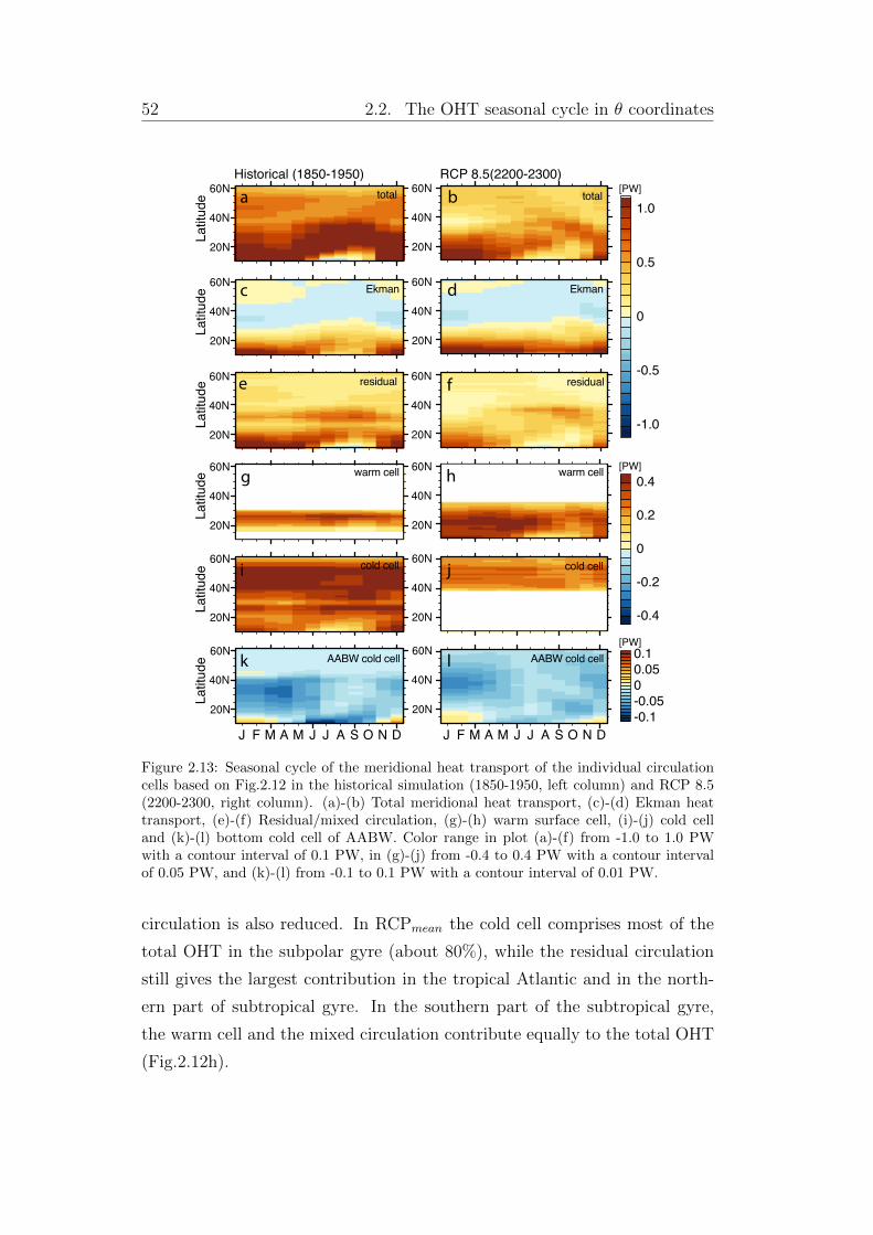
52 2.2. The OHT seasonal cycle in ✓ coordinates
total
Ekman
AABW cold cell
total
Ekman
residual
cold cell
AABW cold cell
cold cell
residual
J F AM M J J A S O N D J F AM M J J A S O N D
0.4
0.2
0
-0.2
-0.4
0.10.050-0.05-0.1
a b
c d
e f
ji
k l
1.0
0.5
0
-0.5
-1.0
warm cellhwarm cellg
Latit
ude
Latit
ude
Latit
ude
Latit
ude
Latit
ude
Latit
ude
[PW]
[PW]
[PW]
Historical (1850-1950) RCP 8.5(2200-2300)
Figure 2.13: Seasonal cycle of the meridional heat transport of the individual circulationcells based on Fig.2.12 in the historical simulation (1850-1950, left column) and RCP 8.5(2200-2300, right column). (a)-(b) Total meridional heat transport, (c)-(d) Ekman heattransport, (e)-(f) Residual/mixed circulation, (g)-(h) warm surface cell, (i)-(j) cold celland (k)-(l) bottom cold cell of AABW. Color range in plot (a)-(f) from -1.0 to 1.0 PWwith a contour interval of 0.1 PW, in (g)-(j) from -0.4 to 0.4 PW with a contour intervalof 0.05 PW, and (k)-(l) from -0.1 to 0.1 PW with a contour interval of 0.01 PW.
circulation is also reduced. In RCPmean the cold cell comprises most of the
total OHT in the subpolar gyre (about 80%), while the residual circulation
still gives the largest contribution in the tropical Atlantic and in the north-
ern part of subtropical gyre. In the southern part of the subtropical gyre,
the warm cell and the mixed circulation contribute equally to the total OHT
(Fig.2.12h).
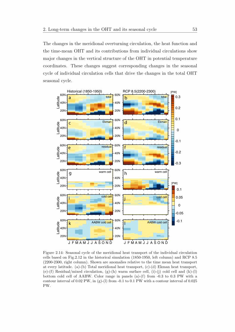
2. Long-term changes in the OHT and its seasonal cycle 53
The changes in the meridional overturning circulation, the heat function and
the time-mean OHT and its contributions from individual circulations show
major changes in the vertical structure of the OHT in potential temperature
coordinates. These changes suggest corresponding changes in the seasonal
cycle of individual circulation cells that drive the changes in the total OHT
seasonal cycle.
Historical (1850-1950) RCP 8.5(2200-2300)
0.1
0.05
0
-0.05
-0.1
0.3
0.2
0.1
0
-0.1
-0.2
-0.3
J F AM M J J A S O N D J F AM M J J A S O N D
total
Ekman
AABW cold cell
total
Ekman
residual
cold cell
AABW cold cell
cold cell
residual
a b
c d
e f
ji
k l
warm cellhwarm cellg
Latit
ude
Latit
ude
Latit
ude
Latit
ude
Latit
ude
Latit
ude
[PW]
[PW]
Figure 2.14: Seasonal cycle of the meridional heat transport of the individual circulationcells based on Fig.2.12 in the historical simulation (1850-1950, left column) and RCP 8.5(2200-2300, right column). Shown are anomalies relative to the time mean heat transportat every latitude. (a)-(b) Total meridional heat transport, (c)-(d) Ekman heat transport,(e)-(f) Residual/mixed circulation, (g)-(h) warm surface cell, (i)-(j) cold cell and (k)-(l)bottom cold cell of AABW. Color range in panels (a)-(f) from -0.3 to 0.3 PW with acontour interval of 0.02 PW, in (g)-(l) from -0.1 to 0.1 PW with a contour interval of 0.025PW.
54 2.2. The OHT seasonal cycle in ✓ coordinates
2.2.3.3 Seasonal cycle of the individual OHT components
The changes in the vertical pathways of the OHT, in the time mean heat
function and especially in the cells of the overturning stream function
describe the changes in the individual contributions to the total OHT
between the historical climate state and RCP8.5 climate and can describe in
turn also the changes in the seasonal cycle of the individual components.
The seasonal cycles of the various circulations contributing to the total
OHT are shown in Fig.2.13 for HISTmean and RCPmean. As shown in
section 2.1 (Fig.2.5), the changes in the seasonal cycle are concealed by
the mean decrease of the OHT amplitude. The OHT seasonal cycle in
HISTmean and RCPmean (Fig.2.13a-b) reveals prominent changes that result
from all of the considered circulation cells (Fig.2.13e-l), although mostly the
cold cell and the residual circulation suggest to force the overall shifts in the
seasonal cycle between HISTmean and RCPmean (Fig.2.13e-f, i-j). Obviously,
the change in the latitudinal and vertical extent of the closed circulations
has a direct impact on the range in the seasonal cycle covered by the
individual circulations.
To emphasize the changes in the OHT seasonal cycle which are
superimposed by the strong reduction of the OHT, anomalies of the
seasonal cycle relative to the annual mean at every latitude are considered
again in the following (Fig.2.14). The seasonal cycle of the total OHT and
the Ekman heat transport (Fig.2.14a-d) reveal the same changes as shown
in section 2.1 with a general northward shift in the pattern of 5 degrees and
temporal shifts between one and six months.
The seasonal cycle of the residual circulation (Fig.2.14e-f) reveals a similar
seasonal cycle, as well as similar shifts in the seasonal cycle from HISTmean
to RCPmean compared to the total OHT. The seasonal cycle in the residual
circulation indicates a generally weaker seasonal cycle than in the total
OHT. The closed circulations generally indicate a much weaker seasonal
cycle with lower seasonal amplitude (Fig.2.14g-l). In HISTmean the warm
cell (Fig.2.14g) covers only a small area between 15�N and 30�N and
indicates a maximum in summer and a minimum in winter – similar to the
2. Long-term changes in the OHT and its seasonal cycle 55
Ekman transport in the subtropical gyre, but with a smaller agreement than
the residual circulation and the Ekman heat transport. In RCPmean the
expansion of the warm cell (Fig.2.14h) leads to an increased influence of the
warm cell seasonal cycle. Following the northward shift of the total OHT
and the Ekman transport the warm cell shows a similar seasonal cycle with
a maximum in winter to spring and a minimum in autumn in the tropics
reaching northward. In contrast to the total OHT and the Ekman heat
transport, the seasonal cycle of the warm cell is almost coherent between
15�N and 35�N and significantly intensified in the seasonal amplitude in
RCPmean.
In HISTmean the seasonal cycle in the cold cell related to the NADW
(Fig.2.14i) is the strongest of the three closed circulations (Fig.2.14g-l). In
the tropical and subtropical North Atlantic, the seasonal cycle in the cold
cell is in phase with the total OHT and the residual circulation, indicating a
barotropic signal of the total heat transport reaching down to the deep
cell. In the subpolar North Atlantic, the seasonal cycle of the cold cell
that establishes here a significant part of the surface circulation is also in
phase with the residual circulation and the total OHT. In RCPmean the
seasonal cycle in the NADW cold cell is restricted to the subpolar gyre and
is significantly reduced. The seasonal cycle is generally shifted to later
months following the phase of the residual circulation and the total OHT,
but still has a low amplitude. In the AABW cold cell the seasonal cycle
contributes only little to the total OHT seasonal cycle and is reduced in
general from HISTmean to RCPmean. The AABW seasonal cycle indicates a
similar northward shift and weakening of the seasonal cycle pattern in the
tropics and subtropics, but with the lowest seasonal amplitude in the closed
circulations.
2.2.4 Summary and Conclusions
The e↵ect of a projected reduction in the Atlantic meridional heat trans-
port (OHT) on the seasonal cycle of the OHT calculated in potential tem-
perature coordinates in a Coupled Model Intercomparison Project phase 5
56 2.2. The OHT seasonal cycle in ✓ coordinates
(CMIP5) climate projection performed in the Max-Planck Institute Earth
System Model (MPI-ESM) is investigated with a focus on the CMIP5 histor-
ical simulation extended with RCP8.5.
The OHT is decomposed based on a heat function in potential tempera-
ture coordinates. We can identify closed circulation cells from the Atlantic
meridional overturning circulation (AMOC) in potential temperature coor-
dinates that imply a meridional heat transport and allow a distinct physical
interpretation of the processes related to the respective closed circulations
of the warm wind-driven surface circulation, two cold circulations related to
the North Atlantic Deep Water (NADW) and the Antarctic Bottom Water
(AABW). The residual to the total OHT yields a residual/mixed circulation
with the influence of both, e↵ects of the wind and of the deep overturning.
The decomposition of the OHT based on the overturning stream function and
the heat function in potential temperature coordinates (Ferrari and Ferreira,
2011) allows to understand changes in the vertical structure of the OHT.
The overall warming of North Atlantic ocean temperatures leads to a shift of
the overturning cell in temperature coordinates to warmer layers of potential
temperature. The heat transport is driven by a warm cell in the subtropical
gyre that expands in meridional direction in RCPmean, and a cold cell that
spans the whole North Atlantic in HISTmean, but weakens and shrinks in
RCPmean due to a reduction in the formation of the NADW. The warm cell
at the surface is thought to be wind driven, while the deep cold cell is associ-
ated with the formation of NADW (Ferrari and Ferreira, 2011). Most of the
heat transport is accomplished by the mixed or residual circulation in both
HISTmean and RCPmean in agreement with Ferrari and Ferreira (2011). The
residual circulation represents the combined e↵ect of the wind-driven circula-
tion and the deep overturning, that cannot be discriminated explicitly. The
AABW cold cell contribution can be neglected for the mean OHT.
The analysis of the OHT based on the heat function reveals changes in agree-
ment with those found in section 2.1. A similar distribution of the OHT in
terms of the heat functions is found in the seasonal cycle. The OHT reveals a
northward shift by about 5� and temporal shifts of 1-6 months in the seasonal
cycle in concert with the shift in the Ekman heat transport seasonal cycle.
The warm cell only contributes in the subtropical gyre, where the seasonal cy-
2. Long-term changes in the OHT and its seasonal cycle 57
cle reveals an increased seasonal amplitude from HISTmean to RCPmean. The
seasonal cycle in the cold cell contributes in HISTmean, but is mostly absent
in RCPmean in the subtropical gyre. In agreement with the time mean OHT,
the seasonal cycle is predominately driven by the residual circulation. Con-
sequently, the changes seen in the seasonal cycle of the OHT can be related
to changes in the wind-driven circulation of the warm cell and to changes
in the formation of NADW in the cold cell, but the major changes appear
in the residual circulation that does not allow a clear separation of wind-
driven e↵ects and e↵ects of changes in the North Atlantic density field. Clear
mechanisms cannot be identified due to the mixed character of the residual
circulation the is driven by both, shallow the wind driven circulation and the
deep overturning. The AABW related cold circulation generally indicates a
weak seasonal cycle, but also shifts from the historical simulation to RCP8.5
which might be associated with changes in the dynamics in the Southern
Ocean. Thus, a combined e↵ect the wind forcing and the deep overturning
mainly leads to the changes seen in the OHT seasonal cycle.
Despite the physical insight obtained from the OHT in potential tempera-
ture coordinates, this decomposition is not considered further in the following
analysis for practical reasons. The decomposition of the OHT based on the
heat function demands for the knowledge and analysis of the full overturning
cell. For the analysis of the predictability in chapter 4, the cells of the over-
turning circulation have to be identified in individual ensemble members of
the hindcast experiments together with the control simulations. The struc-
ture of the closed overturning cells and the heat function have to be evaluated
individually, but might di↵er for the ensemble members, which leads to ad-
ditional uncertainties in the prediction. Further, such a decomposition can
hardly be obtained from observations so that the use and applicability of the
heat function, e.g. in an operational prediction system, might be dubious.

3 Near-term changes in the
seasonal cycle of the Atlantic
meridional heat transport
and the Atlantic meridional
overturning circulation
3.1 Introduction
Changes in the seasonal cycle of the Atlantic meridional heat transport in
the long term until the end of the 23rd century presented in section 2.1
result from a continous increase of surface temperatures and in concert with
a gradual decrease in the AMOC and the OHT starting in the 20th century
of the historical simulation. As a prerequisite for the predictability analysis
in section 4, I here repeat and extend parts of the analysis of chapter 2.1 for
near future changes in the OHT seasonal cycle and for near future changes in
the AMOC seasonal cycle in the MPI-ESM CMIP5 climate projections until
the middle of the 21st century. I aim to find imprints of global warming on
the OHT seasonal cycle in RCP8.5 and additionally in RCP4.5 not only on
centennial time scales, but also on shorter decadal time scales in MPI-ESM.
In the middle of 21st century, North Atlantic SSTs are projected to increase
between about 0.5�C in RCP2.6 to about 2�C in RCP8.5 until 2100 in the
60 3.2. Methods
CMIP5 multimodel ensemble (e.g. IPCC, 2013, Villarini and Vecchi, 2012).
Until 2050, the RCP8.5 scenario in MPI-ESM indicates a global mean
temperature increase by more than 2�C and a reduction in the AMOC
and OHT by 10-20% compared to the historical simulation. Similarly,
the RCP4.5 scenario indicates a global temperature increase of almost
2�C and a reduction of the AMOC and OHT by about 10%. Following
the CMIP5 specifications, the RCP scenarios do not diverge much in the
global response to climate changes until about 2035 (e.g., Meehl et al.,
2012) and are still close to each other until the middle of the 21st century.
Thus, comparable changes for the OHT and AMOC seasonal cycle can be
expected in RCP4.5 and RCP8.5 until the middle of the 21st century.
3.2 Methods
Following section 2.1, the analysis of short term changes in the OHT seasonal
cycle is based on the decomposition of the OHT into overturning and gyre
component (Eq. 2.4, H ⇡ Hov +Hgyre). Additionally, I analyze changes in
the seasonal cycle in the AMOC, that is considered here as the maximum of
the stream function given by (y, z) =0Rz
xER
xW
v(x, y, z) dx dz, the Ekman
transport ek given by ek = � 1
⇢0f
xER
xW
⌧x dx with ⌧x the zonal wind stress at
the ocean surface, and the geostrophic contribution to the AMOC geo which
is approximated here by the AMOC with the Ekman transport removed from
it (AMOC-Ekman): geo ⇡ � ek.
For the analysis, I consider anomalies of the seasonal cycle relative to the
time-mean AMOC and OHT at every latitude. The seasonal anomalies are
considered for the present climate state in the CMIP5 historical simulation
(1850-1950, HISTmean) and for the middle of the 21st century in RCP4.5 and
RCP8.5 (2045-2075).
Additionally, I look at latitude-dependent changes in the peak-to-peak ampli-
tude of the seasonal cycles of AMOC and OHT over the considered periods.
3. Near-term changes in the OHT and AMOC seasonal cycle 61
The peak-to-peak amplitude is defined here by the di↵erence between the
maximum and the minimum of the seasonal cycle depending on latitude.
Further, latitude-dependent temporal shifts in the minima and maxima in
the seasonal cycles of the AMOC and OHT and their components are ana-
lyzed, that give the shift in months for the respective minima and maxima
at every latitude.
3.3 Changes in the seasonal cycle of the
AMOC and the OHT until the middle of
the 21st century
The AMOC and the OHT seasonal cycles and its components reveal changes
with shifts in space and time until the middle of the 21st century in both the
RCP4.5 and the RCP8.5 scenario (Fig.3.1,3.2). Until the middle of the 21st
century, the changes in the AMOC seasonal cycle are roughly comparable be-
tween RCP4.5 and RCP8.5 (Fig.3.1a-c). Both scenarios indicate on average
a slight northward shift of the maximum westerlies at the surface, whereas
no significant expansion of the Hadley cell is found in the time mean (not
shown). But during summer and winter a noticeable poleward expansion of
the Hadley cell by about one to two degrees and a poleward shift of the jet
emerges (not shown). The AMOC seasonal cycle indicates a slight northward
shift of the pattern which is easily visible in the maximum in winter and the
minimum in summer in RCP4.5 and RCP8.5 in the tropical North Atlantic
(Fig.3.1a-c). In addition to the northward shift, single latitudes indicate
changes in the peak-to-peak amplitude and temporal shifts. The decompo-
sition of the AMOC into geostrophic transport and Ekman transport (Fig.
3.1d-i) reveals that the Ekman transport largely contributes to the changes
in the AMOC seasonal cycle.
Similar to the AMOC seasonal cycle, the changes in the total OHT sea-
sonal cycle are comparable between RCP4.5 and RCP8.5 until the middle
of the 21st century (Fig.3.2a-c). Following the northward shift in the atmo-
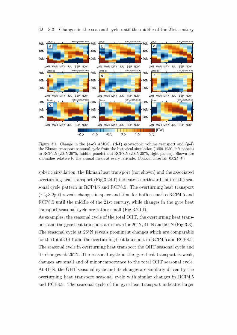
62 3.3. Changes in the seasonal cycle until the middle of the 21st century
d
a b
e
g h
c
f
i
[PW]
Figure 3.1: Change in the (a-c) AMOC, (d-f) geostrophic volume transport and (g-i)the Ekman transport seasonal cycle from the historical simulation (1850-1950, left panels)to RCP4.5 (2045-2075, middle panels) and RCP8.5 (2045-2075, right panels). Shown areanomalies relative to the annual mean at every latitude. Contour interval: 0.02PW .
spheric circulation, the Ekman heat transport (not shown) and the associated
overturning heat transport (Fig.3.2d-f) indicate a northward shift of the sea-
sonal cycle pattern in RCP4.5 and RCP8.5. The overturning heat transport
(Fig.3.2g-i) reveals changes in space and time for both scenarios RCP4.5 and
RCP8.5 until the middle of the 21st century, while changes in the gyre heat
transport seasonal cycle are rather small (Fig.3.2d-f).
As examples, the seasonal cycle of the total OHT, the overturning heat trans-
port and the gyre heat transport are shown for 26�N, 41�N and 50�N (Fig.3.3).
The seasonal cycle at 26�N reveals prominent changes which are comparable
for the total OHT and the overturning heat transport in RCP4.5 and RCP8.5.
The seasonal cycle in overturning heat transport the OHT seasonal cycle and
its changes at 26�N. The seasonal cycle in the gyre heat transport is weak,
changes are small and of minor importance to the total OHT seasonal cycle.
At 41�N, the OHT seasonal cycle and its changes are similarly driven by the
overturning heat transport seasonal cycle with similar changes in RCP4.5
and RCP8.5. The seasonal cycle of the gyre heat transport indicates larger
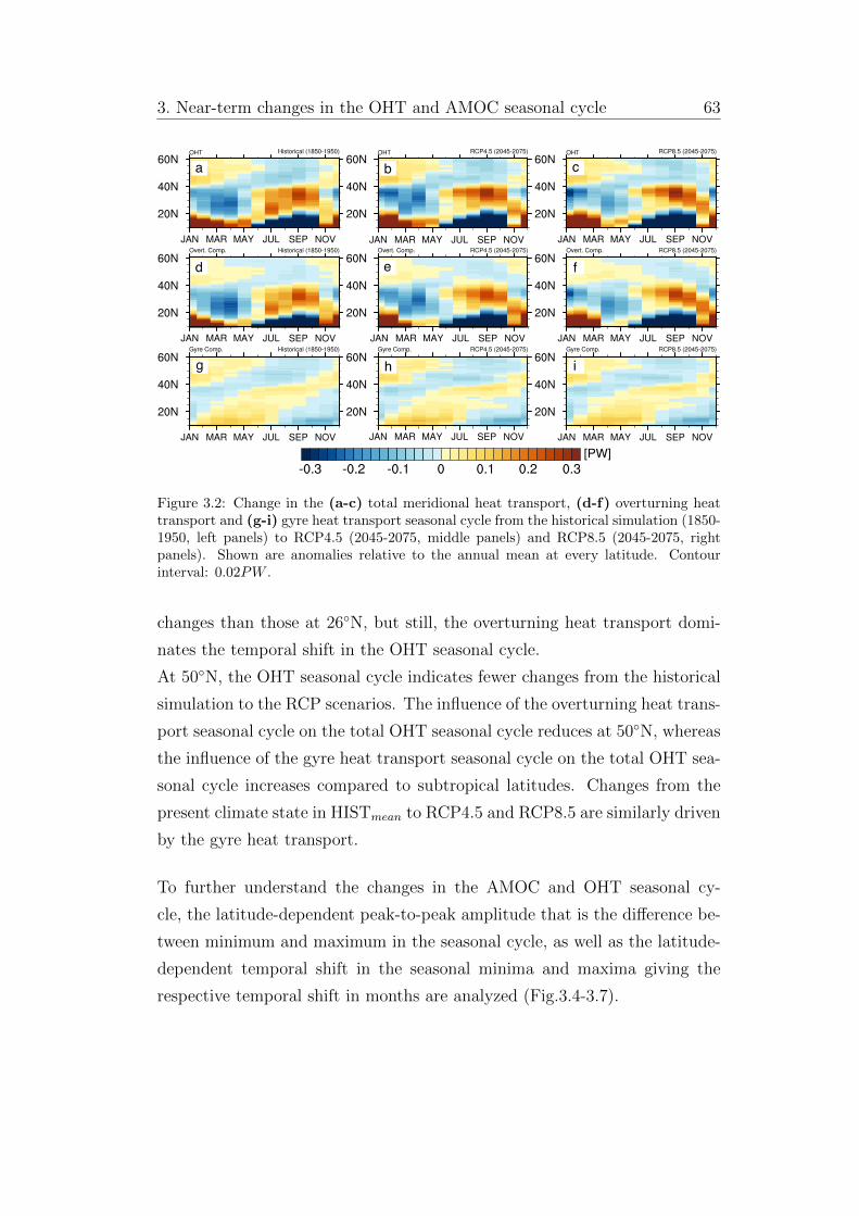
3. Near-term changes in the OHT and AMOC seasonal cycle 63
d
a b
e
g h
c
f
i
[PW]
Figure 3.2: Change in the (a-c) total meridional heat transport, (d-f) overturning heattransport and (g-i) gyre heat transport seasonal cycle from the historical simulation (1850-1950, left panels) to RCP4.5 (2045-2075, middle panels) and RCP8.5 (2045-2075, rightpanels). Shown are anomalies relative to the annual mean at every latitude. Contourinterval: 0.02PW .
changes than those at 26�N, but still, the overturning heat transport domi-
nates the temporal shift in the OHT seasonal cycle.
At 50�N, the OHT seasonal cycle indicates fewer changes from the historical
simulation to the RCP scenarios. The influence of the overturning heat trans-
port seasonal cycle on the total OHT seasonal cycle reduces at 50�N, whereas
the influence of the gyre heat transport seasonal cycle on the total OHT sea-
sonal cycle increases compared to subtropical latitudes. Changes from the
present climate state in HISTmean to RCP4.5 and RCP8.5 are similarly driven
by the gyre heat transport.
To further understand the changes in the AMOC and OHT seasonal cy-
cle, the latitude-dependent peak-to-peak amplitude that is the di↵erence be-
tween minimum and maximum in the seasonal cycle, as well as the latitude-
dependent temporal shift in the seasonal minima and maxima giving the
respective temporal shift in months are analyzed (Fig.3.4-3.7).
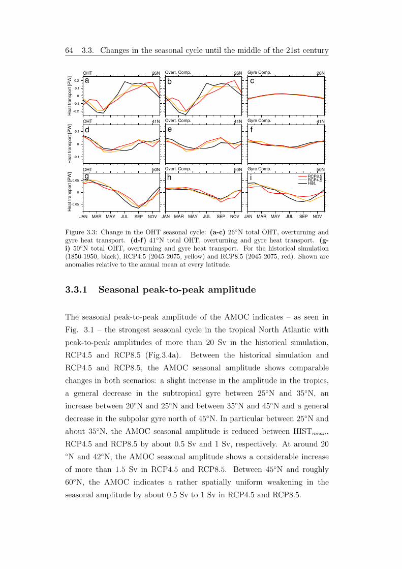
64 3.3. Changes in the seasonal cycle until the middle of the 21st century
a b c
d e f
g h i
Figure 3.3: Change in the OHT seasonal cycle: (a-c) 26�N total OHT, overturning andgyre heat transport. (d-f) 41�N total OHT, overturning and gyre heat transport. (g-i) 50�N total OHT, overturning and gyre heat transport. For the historical simulation(1850-1950, black), RCP4.5 (2045-2075, yellow) and RCP8.5 (2045-2075, red). Shown areanomalies relative to the annual mean at every latitude.
3.3.1 Seasonal peak-to-peak amplitude
The seasonal peak-to-peak amplitude of the AMOC indicates – as seen in
Fig. 3.1 – the strongest seasonal cycle in the tropical North Atlantic with
peak-to-peak amplitudes of more than 20 Sv in the historical simulation,
RCP4.5 and RCP8.5 (Fig.3.4a). Between the historical simulation and
RCP4.5 and RCP8.5, the AMOC seasonal amplitude shows comparable
changes in both scenarios: a slight increase in the amplitude in the tropics,
a general decrease in the subtropical gyre between 25�N and 35�N, an
increase between 20�N and 25�N and between 35�N and 45�N and a general
decrease in the subpolar gyre north of 45�N. In particular between 25�N and
about 35�N, the AMOC seasonal amplitude is reduced between HISTmean,
RCP4.5 and RCP8.5 by about 0.5 Sv and 1 Sv, respectively. At around 20�N and 42�N, the AMOC seasonal amplitude shows a considerable increase
of more than 1.5 Sv in RCP4.5 and RCP8.5. Between 45�N and roughly
60�N, the AMOC indicates a rather spatially uniform weakening in the
seasonal amplitude by about 0.5 Sv to 1 Sv in RCP4.5 and RCP8.5.
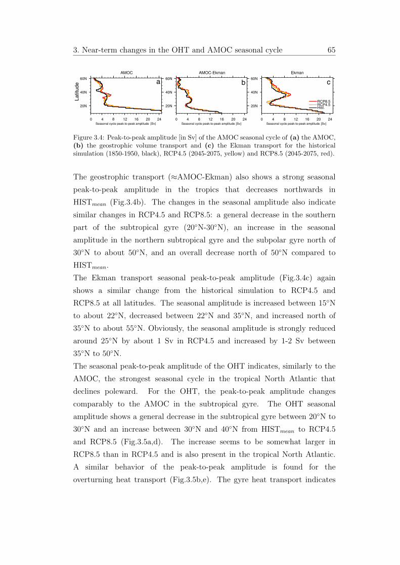
3. Near-term changes in the OHT and AMOC seasonal cycle 65
a b c
[Sv] [Sv] [Sv]
Latitude
Figure 3.4: Peak-to-peak amplitude [in Sv] of the AMOC seasonal cycle of (a) the AMOC,(b) the geostrophic volume transport and (c) the Ekman transport for the historicalsimulation (1850-1950, black), RCP4.5 (2045-2075, yellow) and RCP8.5 (2045-2075, red).
The geostrophic transport (⇡AMOC-Ekman) also shows a strong seasonal
peak-to-peak amplitude in the tropics that decreases northwards in
HISTmean (Fig.3.4b). The changes in the seasonal amplitude also indicate
similar changes in RCP4.5 and RCP8.5: a general decrease in the southern
part of the subtropical gyre (20�N-30�N), an increase in the seasonal
amplitude in the northern subtropical gyre and the subpolar gyre north of
30�N to about 50�N, and an overall decrease north of 50�N compared to
HISTmean.
The Ekman transport seasonal peak-to-peak amplitude (Fig.3.4c) again
shows a similar change from the historical simulation to RCP4.5 and
RCP8.5 at all latitudes. The seasonal amplitude is increased between 15�N
to about 22�N, decreased between 22�N and 35�N, and increased north of
35�N to about 55�N. Obviously, the seasonal amplitude is strongly reduced
around 25�N by about 1 Sv in RCP4.5 and increased by 1-2 Sv between
35�N to 50�N.
The seasonal peak-to-peak amplitude of the OHT indicates, similarly to the
AMOC, the strongest seasonal cycle in the tropical North Atlantic that
declines poleward. For the OHT, the peak-to-peak amplitude changes
comparably to the AMOC in the subtropical gyre. The OHT seasonal
amplitude shows a general decrease in the subtropical gyre between 20�N to
30�N and an increase between 30�N and 40�N from HISTmean to RCP4.5
and RCP8.5 (Fig.3.5a,d). The increase seems to be somewhat larger in
RCP8.5 than in RCP4.5 and is also present in the tropical North Atlantic.
A similar behavior of the peak-to-peak amplitude is found for the
overturning heat transport (Fig.3.5b,e). The gyre heat transport indicates
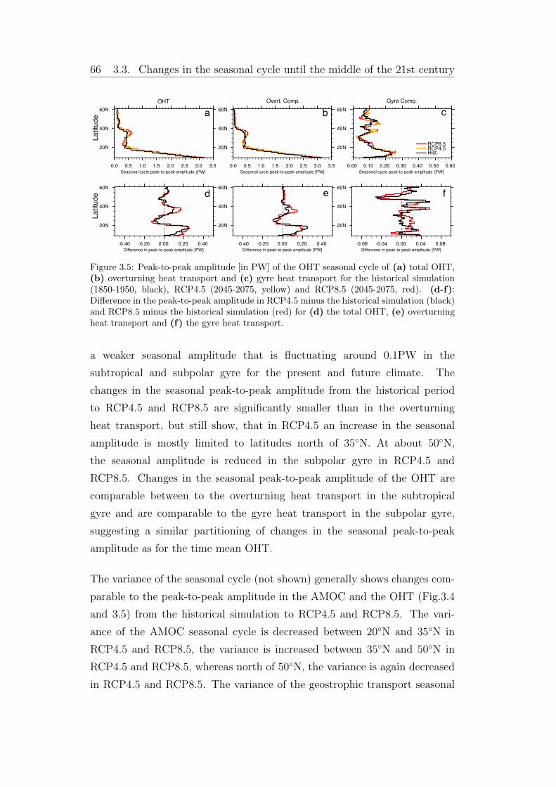
66 3.3. Changes in the seasonal cycle until the middle of the 21st century
a b c
d e f
[PW] [PW] [PW]
[PW] [PW] [PW]
Latitude
Latitude
Figure 3.5: Peak-to-peak amplitude [in PW] of the OHT seasonal cycle of (a) total OHT,(b) overturning heat transport and (c) gyre heat transport for the historical simulation(1850-1950, black), RCP4.5 (2045-2075, yellow) and RCP8.5 (2045-2075, red). (d-f):Di↵erence in the peak-to-peak amplitude in RCP4.5 minus the historical simulation (black)and RCP8.5 minus the historical simulation (red) for (d) the total OHT, (e) overturningheat transport and (f) the gyre heat transport.
a weaker seasonal amplitude that is fluctuating around 0.1PW in the
subtropical and subpolar gyre for the present and future climate. The
changes in the seasonal peak-to-peak amplitude from the historical period
to RCP4.5 and RCP8.5 are significantly smaller than in the overturning
heat transport, but still show, that in RCP4.5 an increase in the seasonal
amplitude is mostly limited to latitudes north of 35�N. At about 50�N,
the seasonal amplitude is reduced in the subpolar gyre in RCP4.5 and
RCP8.5. Changes in the seasonal peak-to-peak amplitude of the OHT are
comparable between to the overturning heat transport in the subtropical
gyre and are comparable to the gyre heat transport in the subpolar gyre,
suggesting a similar partitioning of changes in the seasonal peak-to-peak
amplitude as for the time mean OHT.
The variance of the seasonal cycle (not shown) generally shows changes com-
parable to the peak-to-peak amplitude in the AMOC and the OHT (Fig.3.4
and 3.5) from the historical simulation to RCP4.5 and RCP8.5. The vari-
ance of the AMOC seasonal cycle is decreased between 20�N and 35�N in
RCP4.5 and RCP8.5, the variance is increased between 35�N and 50�N in
RCP4.5 and RCP8.5, whereas north of 50�N, the variance is again decreased
in RCP4.5 and RCP8.5. The variance of the geostrophic transport seasonal
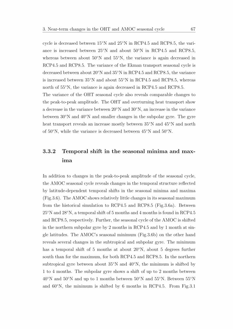
3. Near-term changes in the OHT and AMOC seasonal cycle 67
cycle is decreased between 15�N and 25�N in RCP4.5 and RCP8.5, the vari-
ance is increased between 25�N and about 50�N in RCP4.5 and RCP8.5,
whereas between about 50�N and 55�N, the variance is again decreased in
RCP4.5 and RCP8.5. The variance of the Ekman transport seasonal cycle is
decreased between about 20�N and 35�N in RCP4.5 and RCP8.5, the variance
is increased between 35�N and about 55�N in RCP4.5 and RCP8.5, whereas
north of 55�N, the variance is again decreased in RCP4.5 and RCP8.5.
The variance of the OHT seasonal cycle also reveals comparable changes to
the peak-to-peak amplitude. The OHT and overturning heat transport show
a decrease in the variance between 20�N and 30�N, an increase in the variance
between 30�N and 40�N and smaller changes in the subpolar gyre. The gyre
heat transport reveals an increase mostly between 35�N and 45�N and north
of 50�N, while the variance is decreased between 45�N and 50�N.
3.3.2 Temporal shift in the seasonal minima and max-
ima
In addition to changes in the peak-to-peak amplitude of the seasonal cycle,
the AMOC seasonal cycle reveals changes in the temporal structure reflected
by latitude-dependent temporal shifts in the seasonal minima and maxima
(Fig.3.6). The AMOC shows relatively little changes in its seasonal maximum
from the historical simulation to RCP4.5 and RCP8.5 (Fig.3.6a). Between
25�N and 28�N, a temporal shift of 5 months and 4 months is found in RCP4.5
and RCP8.5, respectively. Further, the seasonal cycle of the AMOC is shifted
in the northern subpolar gyre by 2 months in RCP4.5 and by 1 month at sin-
gle latitudes. The AMOC’s seasonal minimum (Fig.3.6b) on the other hand
reveals several changes in the subtropical and subpolar gyre. The minimum
has a temporal shift of 5 months at about 20�N, about 5 degrees further
south than for the maximum, for both RCP4.5 and RCP8.5. In the northern
subtropical gyre between about 35�N and 40�N, the minimum is shifted by
1 to 4 months. The subpolar gyre shows a shift of up to 2 months between
40�N and 50�N and up to 1 months between 50�N and 55�N. Between 55�N
and 60�N, the minimum is shifted by 6 months in RCP4.5. From Fig.3.1
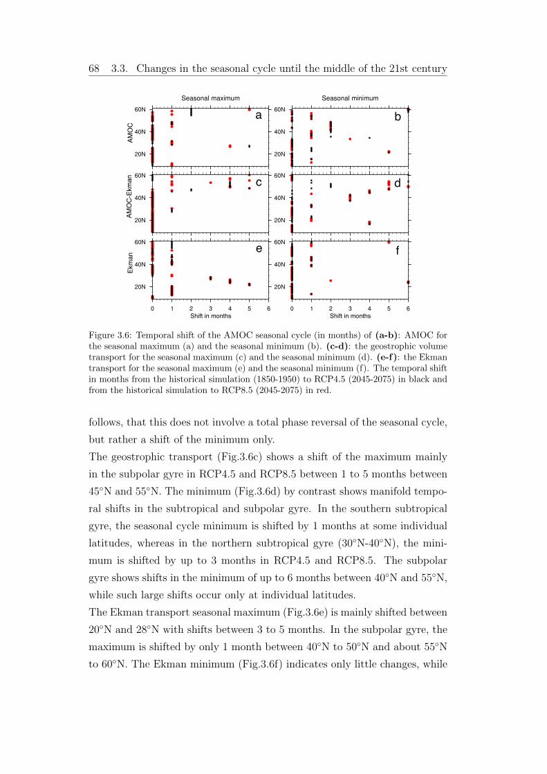
68 3.3. Changes in the seasonal cycle until the middle of the 21st century
Shift in months Shift in months
AM
OC
AM
OC
-Ekm
an
Ekm
an
a
c
e f
b
d
Figure 3.6: Temporal shift of the AMOC seasonal cycle (in months) of (a-b): AMOC forthe seasonal maximum (a) and the seasonal minimum (b). (c-d): the geostrophic volumetransport for the seasonal maximum (c) and the seasonal minimum (d). (e-f): the Ekmantransport for the seasonal maximum (e) and the seasonal minimum (f). The temporal shiftin months from the historical simulation (1850-1950) to RCP4.5 (2045-2075) in black andfrom the historical simulation to RCP8.5 (2045-2075) in red.
follows, that this does not involve a total phase reversal of the seasonal cycle,
but rather a shift of the minimum only.
The geostrophic transport (Fig.3.6c) shows a shift of the maximum mainly
in the subpolar gyre in RCP4.5 and RCP8.5 between 1 to 5 months between
45�N and 55�N. The minimum (Fig.3.6d) by contrast shows manifold tempo-
ral shifts in the subtropical and subpolar gyre. In the southern subtropical
gyre, the seasonal cycle minimum is shifted by 1 months at some individual
latitudes, whereas in the northern subtropical gyre (30�N-40�N), the mini-
mum is shifted by up to 3 months in RCP4.5 and RCP8.5. The subpolar
gyre shows shifts in the minimum of up to 6 months between 40�N and 55�N,
while such large shifts occur only at individual latitudes.
The Ekman transport seasonal maximum (Fig.3.6e) is mainly shifted between
20�N and 28�N with shifts between 3 to 5 months. In the subpolar gyre, the
maximum is shifted by only 1 month between 40�N to 50�N and about 55�N
to 60�N. The Ekman minimum (Fig.3.6f) indicates only little changes, while
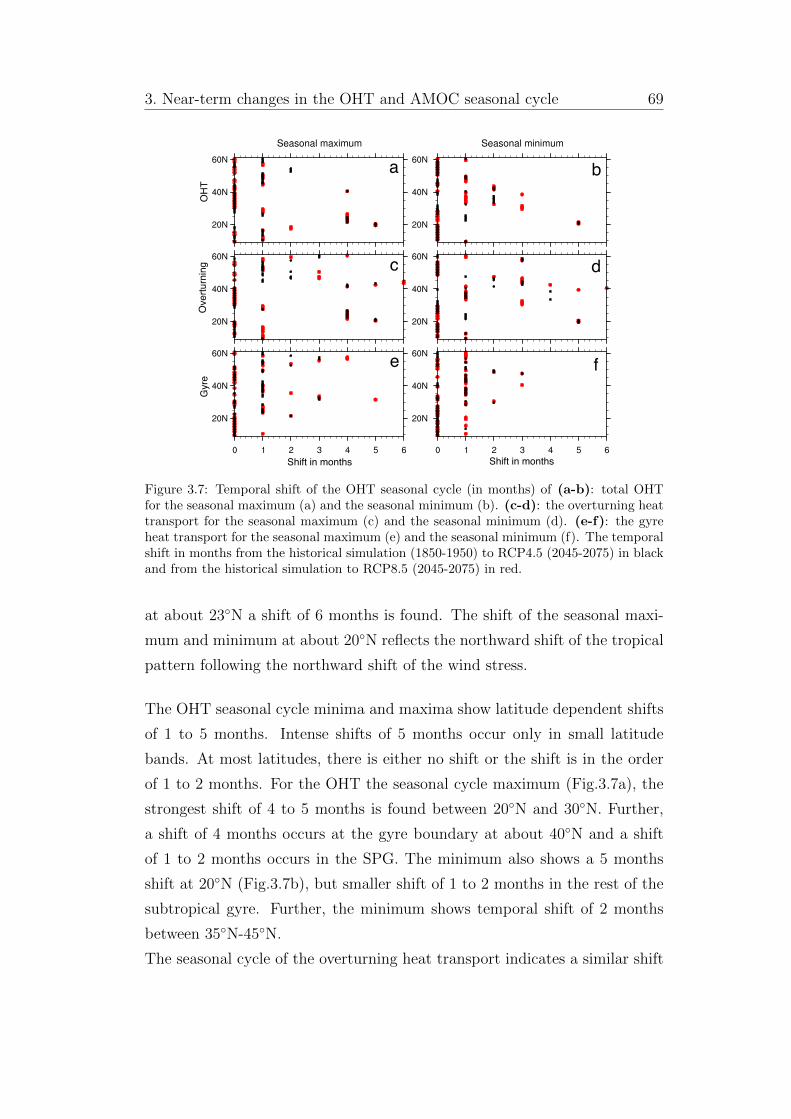
3. Near-term changes in the OHT and AMOC seasonal cycle 69
a
c
e f
d
b
Shift in months Shift in months
OHT
Ove
rturn
ing
Gyr
e
Figure 3.7: Temporal shift of the OHT seasonal cycle (in months) of (a-b): total OHTfor the seasonal maximum (a) and the seasonal minimum (b). (c-d): the overturning heattransport for the seasonal maximum (c) and the seasonal minimum (d). (e-f): the gyreheat transport for the seasonal maximum (e) and the seasonal minimum (f). The temporalshift in months from the historical simulation (1850-1950) to RCP4.5 (2045-2075) in blackand from the historical simulation to RCP8.5 (2045-2075) in red.
at about 23�N a shift of 6 months is found. The shift of the seasonal maxi-
mum and minimum at about 20�N reflects the northward shift of the tropical
pattern following the northward shift of the wind stress.
The OHT seasonal cycle minima and maxima show latitude dependent shifts
of 1 to 5 months. Intense shifts of 5 months occur only in small latitude
bands. At most latitudes, there is either no shift or the shift is in the order
of 1 to 2 months. For the OHT the seasonal cycle maximum (Fig.3.7a), the
strongest shift of 4 to 5 months is found between 20�N and 30�N. Further,
a shift of 4 months occurs at the gyre boundary at about 40�N and a shift
of 1 to 2 months occurs in the SPG. The minimum also shows a 5 months
shift at 20�N (Fig.3.7b), but smaller shift of 1 to 2 months in the rest of the
subtropical gyre. Further, the minimum shows temporal shift of 2 months
between 35�N-45�N.
The seasonal cycle of the overturning heat transport indicates a similar shift
70 3.4. Summary
in the seasonal maxima in the subtropical North Atlantic with shifts of 4 to 5
months between 20�N-30�N and 1 to 3 months in the subpolar gyre (Fig.3.7c).
The minimum is also shifted by 1 to 4 months in the subpolar gyre with
prominent changes between 40�N and 45�N (Fig.3.7d). In the subpolar gyre
the temporal shift of the minima and maxima is even larger than for the OHT
with a shift in the minimum up to 3 months at . The seasonal cycle of the gyre
heat transport shows generally smaller temporal shifts limited to 3 months at
about 35�N and 55�N for the seasonal maximum and at 50�N for the seasonal
minimum. Overall, the OHT seasonal cycle is considerably shifted between
20�N to 25�N and 35�N to 45�N. The overturning heat transport is mainly
shifted between 20�N and 30�N and roughly between 40�N and 60�N. The
gyre heat transport seasonal cycle reveals the overall smallest shifts.
3.4 Summary
Compared to the longterm changes in RCP8.5 (section 2.1) similar albeit
less intense changes in the seasonal cycle pattern of the OHT can already be
identified in the middle of the 21st century in RCP4.5 and RCP8.5. Further,
the AMOC also reveals latitude-dependent changes its seasonal cycle.
The AMOC shows a general decrease in the seasonal peak-to-peak ampli-
tude in the subtropical gyre and large parts of the subpolar gyre. The large
decrease in the seasonal amplitude appears in the subtropical gyre at about
25�-30�N similar to the latitudes where the maximum is strongly shifted. In
the subpolar gyre, the geostrophic transport indicates temporal shifts that
might be evidence of changes in the AMOC seasonal cycle, especially in the
seasonal minimum. The changes in the Ekman transport seasonal cycle are
rather small and mainly project on the AMOC seasonal cycle at southern
latitudes of the subtropical gyre.
The OHT, the overturning heat transport and the gyre heat transport also
reveal changes depending on latitude. The overturning heat transport sea-
sonal cycle shows that changes in the seasonal amplitude are prominent in
the subtropical gyre, influencing the OHT seasonal cycle here. Coupled to
3. Near-term changes in the OHT and AMOC seasonal cycle 71
this, changes in the variance of the seasonal cycle of the overturning heat
transport are pronounced in the subtropical gyre, indicating changes in the
seasonal variability. Mostly between 20�N and about 40�N, the overturning
heat transport controls the temporal shift in the OHT seasonal cycle. The
seasonal minima and maxima show shifts in the STG and SPG. The gyre heat
transport influences changes in the OHT seasonal cycle mostly in the subpo-
lar gyre, where the seasonal variability of the gyre heat transport dominates
the seasonal amplitude of the OHT and temporal shifts of up to 3 months
occur mostly between 50�N-60�N.
Overall, in agreement with the longterm changes in the OHT seasonal cycle,
the changes in the amplitude are mostly due to the overturning heat trans-
port seasonal cycle in the subtropical gyre and due to the gyre heat transport
in the subpolar gyre. But shifts in the seasonal minima and maxima appear
in the overturning heat transport predominantly in the subpolar gyre. This
suggests that prominent changes in the dynamics of the seasonal cycle in
both the atmospheric contribution and the oceanic contributions are already
noticeable in the 21st century and intensify continuously until the end of the
23rd century in the model simulation.
The comparison of changes in the AMOC and OHT seasonal cycles indicates
that a direct transfer of changes in the AMOC seasonal cycle on changes
in the OHT seasonal cycle is not obvious, although changes in the seasonal
amplitude are comparable in the subtropical gyre. Temporal shifts, as well
as changes in the seasonal peak-to-peak amplitude di↵er between the AMOC
and the OHT depending on latitude.
3.5 Conclusions
Both, the AMOC and the OHT with all their contributions reveal noticeable
changes in the seasonal cycle from the historical simulation to RCP4.5 and
to RCP8.5.
• The changes in the seasonal cycle give rise to expect changes in the
predictability of the AMOC and the OHT – if these depend on changes
72 3.5. Conclusions
in the variability – especially at latitudes with outstanding temporal
shifts and changes in the peak-to-peak amplitude.
• In particular between 25�N and 35�N in the subtropical gyre, at about
40�N and north of 50�N in the subpolar gyre, the changes in the peak-
to-peak amplitude and the temporal shifts of the seasonal minima and
maxima motivate to expect considerable changes in the predictability
of the AMOC in a future climate state.
• Accordingly, around 25�N, 30�N to 40�N in the subtropical gyre and
between 40�N and 60�N in the subpolar gyre, the identified changes
in the OHT seasonal cycle hint to changes in the predictability of the
OHT in a future climate state.
In particular, the predictability could be influenced at latitudes showing a
reduction in the peak-to-peak amplitude and the variance of the seasonal
cycle what might lead to a reduction in the predictability. But how the
predictability changes at these specific latitudes and how a changed seasonal
cycle influences the predictability of the AMOC and the OHT for yearly and
also for multiyear seasonal means – as winter or summer means – is unclear
and will be investigated in the following chapter.
4 Potential predictability of the
North Atlantic ocean circula-
tion in the present and future
climate
4.1 Introduction
Near-term climate predictions on seasonal to decadal time scales are of grow-
ing interest, not only in the scientific community, but also for stakeholders,
policy makers and decision makers who depend on reliable climate predic-
tions for appropriate decisions. But the field of decadal climate predictions
is still relatively novel and rapidly evolving (e.g., Goddard et al., 2012).
Under global warming, the North Atlantic climate is projected to change
with increased surface temperatures and changes in the circulation of the
atmosphere and the ocean. Together with global warming, the seasonal cy-
cle of surface temperatures (Dwyer et al., 2012), in the arctic ocean (Car-
ton et al., 2015) and also of the Atlantic meridional overturning circulation
(AMOC) and meridional heat transport (OHT) (Chapter 2 and 3) is pro-
jected to change. Whether global warming and especially the changes in
the seasonal cycle impact the predictability is mostly unknown. Boer (2009)
found a decrease in the potential (decadal) predictability of surface temper-
atures and precipitation and Tietsche et al. (2013) found a reduction in skill
74 4.1. Introduction
of Arctic sea ice predictions under global warming. However, whether global
warming a↵ects the predictability of the AMOC and the OHT has not yet
been investigated. Here I investigate changes in the potential predictability
of the AMOC and the OHT between a present climate state based on the
CMIP5 historical simulation and a future climate state in the middle of the
21st century based on RCP4.5.
The North Atlantic Ocean plays a fundamental role in the North Atlantic
climate and its variability and has been shown to impact the European and
North American climate (e.g., Sutton and Hodson, 2005, Knight et al., 2005,
Pohlmann et al., 2006). Thus, the key role of the North Atlantic motivates to
advance the understanding of the North Atlantic climate predictability, even
though the specific role of the North Atlantic Ocean is still controversially
discussed (e.g., Riser and Lozier, 2013).
In context of the recent coordinated e↵ort of the Coupled Model Intercom-
parison Project Phase 5 (CMIP5, Taylor et al., 2012) as part of the fifth as-
sessment report of the Intergovernmental Panel on Climate Change (IPCC),
decadal climate predictions have been investigated in a multi-model frame-
work based on a large ensemble of coupled climate model simulations. The
analysis of predictability relies on retrospective ensemble forecast experi-
ments, so-called ensemble hindcast experiments. Studies in the context of
CMIP5 mostly focussed on the analysis of the predictability under historical
climate conditions that represent the climate state of the last half century
from 1960 to the beginning of the 21st century (Meehl et al., 2009).
Predictability on decadal scales has been found for a number of climate vari-
ables, such as air and sea surface temperatures (e.g., Pohlmann et al., 2009,
van Oldenborgh et al., 2012), the North Atlantic subpolar gyre (e.g., Matei
et al., 2012b, Yeager et al., 2012, Robson et al., 2012), the AMOC (e.g.,
Collins et al., 2006, Msadek et al., 2010, Matei et al., 2012a, Pohlmann et al.,
2013b) and OHT (e.g., Tiedje et al., 2012) and is assessed in either potential
predictability or actual forecast skill.
Most predictability studies have focussed on the analysis of multi-year means.
However, climate variables as well as the underlying mechanisms change sea-
sonally in space and time and thus, the predictability might vary between
4. Potential predictability in the present and future climate 75
di↵erent seasons. Muller et al. (2012) and MacLeod et al. (2012) analyzed
the predictive skill of multiyear seasonal means of surface air temperatures
and precipitation. MacLeod et al. (2012) found that yearly means yield higher
skill than multiyear seasonal means. Yet, the predictability of multiyear sea-
sonal means has not been examined for the AMOC and the OHT and might
give valuable insights concerning the impact of changes in the seasonal cycle
on the predictability.
Forecast skill in these experiments is usually assessed from metrics like the
root-mean-square error (RMSE), anomaly correlation coe�cient (ACC) or
the ensemble spread and for the skill of initialized prediction experiments
compared to uninitialized predictions (Collins, 2002, Collins and Allen, 2002,
Collins and Sinha, 2003, Pohlmann et al., 2004, Msadek et al., 2010). By the
direct comparison of uninitialized and initialized predictions in terms of skill
scores, areas emerge where initialization increases the skill (e.g., Meehl et al.,
2014).
Considering the process of decision making, predictions need to be skillful
and additionally reliable – meaning that predictions might have a value for
the decision making process (Corti et al., 2012). A reliable forecast implies,
that the forecast probabilities for one specific event match the observed fre-
quencies for that specific event. In other words, if a prediction is unreliable,
the information obtained from the prediction might be misleading and causes
inappropriate decisions.
Reliability is traditionally assessed in weather forecasts or seasonal predic-
tions for a specific event that could be the temperature or precipitation above
a certain threshold (e.g., Palmer et al., 2008, Weisheimer and Palmer, 2014).
Recently, the reliable of decadal predictions was investigated for the first
time, showing that for some regions reliable decadal predictions are possible
for surface temperatures, even though the reliability is significantly reduced
when the trend is removed from the ensemble (Corti et al., 2012).
Decadal predictions are still in an early stage (Goddard et al., 2013), even
though a lot of progress and success was achieved from CMIP5 (e.g., Meehl
et al., 2014). So far, decadal prediction studies mostly focussed on the his-
torical climate state, but studies invoking the e↵ects of climate change on the
decadal predictability do not exist to my knowledge, except of the study of
76 4.1. Introduction
Boer (2009) and Tietsche et al. (2013). As shown in the previous chapters
2 and 3, global climate change impacts the mean state, the variability and
the seasonal cycle of the AMOC and the OHT on long time scales (until the
end of the 23rd century) and even on shorter time scales until the middle
of the 21st century. Latitude-dependent, significant changes occur until the
middle of the 21st century with changes in the seasonal amplitude and in
the seasonal variability (chapter 3), which might induce changes in the pre-
dictability of the AMOC and OHT from the present to a future climate state.
From these changes found in chapter 3, the following questions concerning
the predictability of the AMOC and OHT arise:
1. Does the potential predictability of the AMOC and the OHT change
between the present climate state and a projected future climate state
in the middle of the 21st century?
2. If so, does the decadal predictability of the AMOC and the OHT change
predominately at those latitudes where the largest changes are found
in the seasonal cycle?
3. How does the decadal predictability change in multiyear seasonal
means? Do specific seasons indicate a stronger influence of global
warming than others and thus impact the predictability of yearly
means?
To answer these issues, I use ensemble prediction experiments with the Max-
Planck-Insitute Earth system model and analyze the potential predictability
of the AMOC and the OHT for a present and a future climate state. The
predictability analysis is based on the CMIP5 historical simulation and the
RCP4.5 scenario in MPI-ESM. The ensemble experiment for the present cli-
mate state (HISTens) extends from 1995 to 2023, using 20 start years with 10
ensemble member per start year. For the experiment HISTens, the historical
simulation is extended with the RCP4.5 scenario after 2005. An equivalent
ensemble experiment is performed for the future climate state in RCP4.5
(RCPens), between 2045 and 2073. In these experiments, the potential pre-
4. Potential predictability in the present and future climate 77
dictability of the AMOC and OHT is analyzed for yearly means and for multi-
year seasonal means. The analysis is conducted using the anomaly correlation
coe�cient (ACC) as deterministic predictability measure, and reliability di-
agrams in combination with the Brier Skill Score (BSS) as a probabilistic
predictability measure in HISTens and RCPens.
4.2 Methods
4.2.1 Model and ensemble generation
The study is based on two ensemble prediction experiments integrated in
the coupled MPI Earth System Model (MPI-ESM; Jungclaus et al., 2013,
Stevens et al., 2013). Since decadal climate predictions are known to be sen-
sitive to perturbations in the initial conditions, a number of methodologies
have been applied (e.g., Baehr and Piontek, 2013, and references therein).
In this study, I initialize the ensemble with breeding of the ocean component
of MPI-ESM to generate optimal perturbations.
To analyze the potential predictability in the North Atlantic, I use CMIP5
experiments (Taylor et al., 2012) performed in MPI-ESM at low resolution.
The atmospheric model (ECHAM6) is run with a resolution of T63 and 47
vertical levels. The ocean component (MPIOM) is run with an average hori-
zontal resolution of about 1.5� and 40 vertical levels.
The initial conditions for the ensemble members in the hindcast experiments
are created based on a method called “breeding of growing modes” (Toth
and Kalnay, 1993, 1997) which has its origin in weather forecasting. For the
breeding, the control simulation (here the historical simulation and RCP4.5
in MPI-ESM) is run a second time over the hindcast period from perturbed
initial conditions starting on the 1st January 1990 and 2040, respectively.
After one rescaling interval (=breeding cycle) – in which the error with re-
spect to the control simulation grows in time – the ocean component of the
breeding run is rescaled by bred vectors to the control simulation. Bred
vectors are computed from the di↵erence between the control run and the
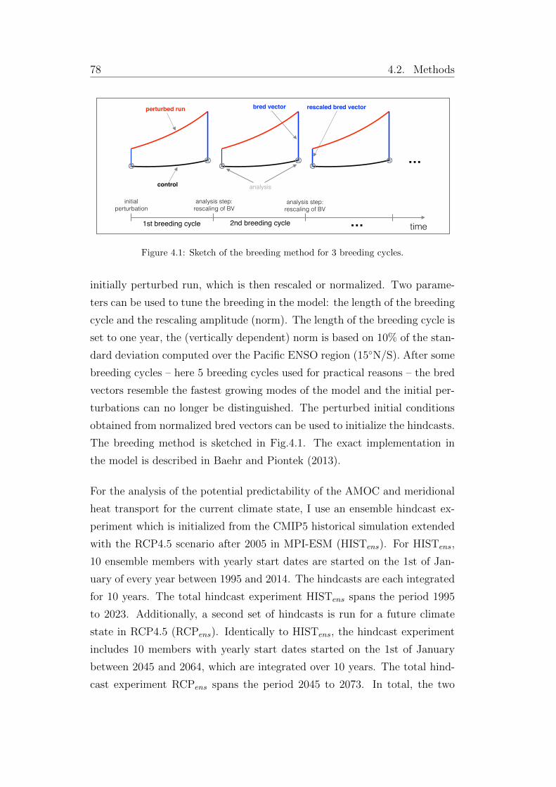
78 4.2. Methods
atmospheric model (ECHAM6) is run with T63 resolution and 47 vertical levels. The ocean
component (MPIOM) is run with an average horizontal resolution of ~1.5° and 40 vertical levels.!
For the analysis of the potential predictability of the AMOC and meridional heat transport for the
current climate state, I use an ensemble hindcast experiment which is initialized from an
assimilation run performed in MPI-ESM. For the assimilation run, first an ocean-only run in
MPIOM is forced with daily NCEP/NCAR reanalysis data (Kalnay et al., 1996). In the coupled
MPI-ESM, the model state is nudged towards three dimensional temperature and salinity
anomalies from the ocean-only run (for details see Matei et al., 2012b), but no assimilation of
atmospheric parameters is done. This assimilation experiment is used for the decadal prediction
system of the MPI-M (Müller et al., 2012). The three-dimensional atmospheric and ocean fields
are then considered for the generation of an ensemble for the beginning of the 21st century
started in the year 2000. !
The initial conditions for the ensemble hindcast experiments are created based on a method
called “breeding of growing modes“ (Toth and Kalnay, 1993,1997) which has its origin in weather
forecasting. For the breeding run the control simulation (here the assimilation run in MPI-ESM) is
run a second time from perturbed initial conditions starting on the 1st January 1997. To calculate
the initial perturbations for the breeding run I use the 1st Jan of the years 1992-1996 from the
assimilation experiment. !
After one rescaling interval (=breeding cycle) – in which the error with respect to the control
simulation grows in time – the ocean component of the breeding run is rescaled by bred vectors
to the control simulation. Bred vectors are computed from the difference between the control run
and the initially perturbed run, which is then rescaled or normalized. Two parameters can be
used to tune the breeding in the model: the length of the breeding cycle and the rescaling
amplitude (norm). The length of the breeding cycle is set to one year, the (vertically dependent)
norm is based on 10% of the standard deviation (??) computed over the Pacific ENSO region
- � -5
- Bred vector (BV): Difference between control and perturbed run!- BV rescaled/normalized after 1 breeding cycle (1 year)
- normalized BV is used for the initial perturbation for the next initialization
- 2 parameters for tuning: time interval (length) of breeding cycle and
rescaling amplitude (norm)
- After some breeding cycles, the bred vectors begin to resemble the
fastest growing modes of the model
bred vector rescaled bred vector
control
perturbed run
analysis
time
initial perturbation
analysis step: rescaling of BV
analysis step: rescaling of BV
1st breeding cycle 2nd breeding cycle …
…
Fig.1: Schematic of the breeding methodFigure 4.1: Sketch of the breeding method for 3 breeding cycles.
initially perturbed run, which is then rescaled or normalized. Two parame-
ters can be used to tune the breeding in the model: the length of the breeding
cycle and the rescaling amplitude (norm). The length of the breeding cycle is
set to one year, the (vertically dependent) norm is based on 10% of the stan-
dard deviation computed over the Pacific ENSO region (15�N/S). After some
breeding cycles – here 5 breeding cycles used for practical reasons – the bred
vectors resemble the fastest growing modes of the model and the initial per-
turbations can no longer be distinguished. The perturbed initial conditions
obtained from normalized bred vectors can be used to initialize the hindcasts.
The breeding method is sketched in Fig.4.1. The exact implementation in
the model is described in Baehr and Piontek (2013).
For the analysis of the potential predictability of the AMOC and meridional
heat transport for the current climate state, I use an ensemble hindcast ex-
periment which is initialized from the CMIP5 historical simulation extended
with the RCP4.5 scenario after 2005 in MPI-ESM (HISTens). For HISTens,
10 ensemble members with yearly start dates are started on the 1st of Jan-
uary of every year between 1995 and 2014. The hindcasts are each integrated
for 10 years. The total hindcast experiment HISTens spans the period 1995
to 2023. Additionally, a second set of hindcasts is run for a future climate
state in RCP4.5 (RCPens). Identically to HISTens, the hindcast experiment
includes 10 members with yearly start dates started on the 1st of January
between 2045 and 2064, which are integrated over 10 years. The total hind-
cast experiment RCPens spans the period 2045 to 2073. In total, the two
4. Potential predictability in the present and future climate 79
hindcast experiments HISTens and RCPens include 200 ensemble members,
respectively.
4.2.2 Predictability analysis
Decadal predictions belong to the category of probabilistic forecasts and their
predictability is often quantified based on deterministic measures like the cor-
relation coe�cient, the mean squared error (MSE) or based on the spread of
the ensemble focussing on the accuracy of the prediction. In this study, the
potential predictability of the AMOC and OHT is quantified depending on
lead time using the anomaly correlation coe�cient (ACC) in a first step,
and using reliability diagrams and the Brier Skill Score (BSS) in a second
step. The analysis is carried out for the present climate state in the histori-
cal ensemble experiment (HISTens, 1995-2023) and a future climate state in
ensemble experiment in RCP4.5 (RCPens, 2045-2073).
Anomaly correlation coe�cient
The anomaly correlation coe�cient (ACC) depending
on latitude and lead time can be calculated from (e.g., Collins, 2002,
Pohlmann et al., 2009, Wilks, 2011):
ACC(t) =
nPi=1
[fi � cf ](t)[o� co]
(i+t)
rnP
i=1
[fi � cf ]2
(t)
nPi=1
[o� co]2
(i+t)
, (4.1)
where t the lead time in years, fi is the ith monthly mean model hindcast and
o the monthly mean control simulation. The control simulation in HISTens is
the historical simulation extended with RCP4.5 for the period 1995 to 2023,
the control simulation in RCPens is RCP4.5 for the period 2045 to 2073. In
contrast to e.g. Pohlmann et al. (2009), anomalies are defined with respect
to the climatologies of the forecast and control simulations cf and co which
80 4.2. Methods
are first removed from the monthly mean data. Afterwards, the ACC is cal-
culated for yearly means (denoted by the overbar) of the anomalies.
Anomalies of the control simulation in the ACC are defined with respect to
the climatology over the respective hindcast period. In particular, in HISTens
anomalies of the control simulation are defined with respect to the 1995-2023
climatology in the historical simulation extended with RCP4.5 after 2005.
In RCPens anomalies of the control simulation are defined with respect to
the 2045-2073 climatology in RCP4.5. For the hindcasts, anomalies are de-
fined with respect to the ensemble mean climatology and lead time with a
“leave-one-out” cross-validation applied to the data (Gangstø et al., 2013).
By applying cross-validation, the considered ensemble member does not con-
tribute to the climatology removed from it. The significance of the ACC is
calculated from a bootstrapping procedure with 1000 iterations at the 95%
confidence level.
In the following the anomaly correlation coe�cient is evaluated for lead years
1 to 10 in HISTens and RCPens for both yearly means and multi-annual sea-
sonal means. The anomalies are removed before yearly and seasonal means
are calculated for the ACC. A linear trend is further removed before the cal-
culation of the ACC to correct for both the forced trend from greenhouse gas
forcing and the unforced model drift in the freely emerging hindcasts.
Both the AMOC and the OHT, as well as their decompositions are analyzed.
The AMOC is decomposed into the wind-driven Ekman transport and the
geostrophic transport (⇡AMOC-Ekman transport). For the predictability
analysis, I focus solely on the geostrophic transport, since the Ekman trans-
port is assumed be little skillful (e.g., von Storch and Haak, 2008). The
OHT is decomposed into overturning heat transport and gyre heat transport
according to Eq.2.4.
Reliability and Brier Skill Score
The limit of deterministic measures is that uncertain-
ties of the prediction are not mirrored in them. Therefore, the reliability
and Brier Skill Score (BSS) of the prediction as a probabilistic measure is
4. Potential predictability in the present and future climate 81
used in addition to the ACC. The analysis of the reliability of a prediction
can be formulated with reliability (or attributes) diagrams (e.g. Palmer
et al., 2008, Corti et al., 2012, Weisheimer and Palmer, 2014) and the Brier
score (Brier, 1950) which are used to determine changes in the predictability
from the historical climate state in HISTens to a future climate state in
RCPens in this study.
Reliability diagrams compare the forecast probabilities of a well-defined
event against the observed statistical frequency with which these events
actually happen. For a perfectly reliable prediction, the forecast probability
equals the observed frequency of an event. The plotted pairs of forecast
probability and observed frequency (=reliability curve) lie on the diagonal
of the reliability diagram (grey line, e.g. in Fig.4.3) and the slope of the
reliability curve is 1 (within the uncertainty) if the prediction is perfectly
reliable. When the slope of the reliability curve is generally positive, the
prediction is thought to have reliability. This means, that with increasing
forecast probabilities, the observed frequency increases. If the reliability
curve is flatter than the diagonal, the prediction is overconfident. However,
if the curve is steeper than the diagonal, the prediction is underconfident. If
the reliability curve is flatter than the no-skill line, the forecast probabilities
cannot be considered to yield significant skill. If the curve is horizontal,
the observed frequency of occurrence does not depend on the forecast
probabilities. In general, the reliability is sensitive to small sample sizes.
Further, the resolution of the reliability diagram is considered and displayed
in sharpness diagrams. The resolution quantifies how much the forecast
probabilities di↵er from the climatological probability of an event. The
higher the resolution, the more the forecast probabilities di↵er from the
climatological probability. In other words, a forecast with a high resolution
should be able to di↵erentiate between high and low probabilities of an
event.
The sharpness diagram shows a histogram of the relative frequency of
the predicted event depending on the bins of the forecast probability. If
bins of the forecast probabilities at the upper and lower bound (with
forecast probabilities close to 0 and 1) of the sharpness diagram show the
highest values, the resolution is high and the prediction is sharp. Ideally,
82 4.2. Methods
predictions should be both: sharp (high resolution) and reliable.
In addition to reliability diagrams, the Brier Skill Score (BSS) is considered
for the reliability of the prediction experiments. The Brier Skill Score can
be calculated from the Brier Score (BS) that is given by (Brier, 1950):
BS =1
N
NX
i=1
(fi � oi)2, (4.2)
with N the number of realizations (pairs of forecast and event), fi the forecast
probability of the ith realization and oi the outcome of the actual event. oi
is equal to 1 if the event occurred and 0 if not. BS measures the accuracy of
a probability forecast in terms of the mean square error. BS ranges between
0 to 1, with BS = 0 giving a perfectly reliable forecast where the forecast
probability equals the outcome of the event.
The Brier Score can be decomposed into three components of uncertainty,
reliability and resolution (Murphy, 1973):
BS =1
N
KX
k=1
nk(fk � ok)2
| {z }REL
� 1
N
KX
k=1
nk(ok � o)2
| {z }RES
+ o(1� o)| {z }UNC
, (4.3)
with N the sample size, K number of probability classes (bins), fk and ok the
forecast probability and observed frequency of an event in bin k and o =NPi=1
oi
N
the overall sample averaged frequency (sample climatology). The first term
(REL) gives the reliability, the second term (RES) the resolution and the
third term (UNC) the uncertainty of the forecast (see also Wilks, 2011).
The reliability term measures the forecast probability against the observed
relative frequency in the considered bins. The smaller the reliability is, the
more reliable the prediction is thought to be. The resolution measures the
the observed relative frequency against the overall sample frequency (sample
climatology). The larger the resolution is, the more reliable are predictions
close the forecast probability of 0 and 1. The uncertainty only depends on
the observations and gives the variability of the observations.
4. Potential predictability in the present and future climate 83
Based on the Brier score BS, the Brier Skill Score (BSS) can be defined:
BSS = �BS � BSref
BSref, (4.4)
with BS the Brier Score of the forecast evaluated against the Brier Score of
a reference forecast BSref . Usually, the sample climatology is used for the
reference forecast, so that the Brier Score can be shown to simplify to:
BSS =RES �REL
UNC. (4.5)
Thus, the BSS can be calculated from the reliability REL, the resolution
RES and the uncertainty UNC of the prediction.
Following Palmer (2000) and Corti et al. (2012), the BSS using the sample
climatology as reference forecast can be decomposed as:
BSS = BSSrel +BSSres � 1, (4.6)
since for a perfectly reliable prediction BSS = BSSrel = BSSres = 1. Here,
the reliability and resolution give two contributions to the Brier Skill Score
(1) BSSrel = 1 � BSrel
BSclim and (2) BSSres = BSres
BSclim , which are used in this
thesis in the subsequent reliability analysis.
Both, reliability diagrams and the Brier Skill Score are evaluated for the
present climate ensemble HISTens and the future climate ensemble RCPens
for lead years 1, 2-3 and 4-5 for multiyear yearly means and multiyear sea-
sonal means. The range of lead years used in this study di↵ers to the set of
time scales suggested by Goddard et al. (2013). However, these timescales
turned out to be a reasonable choice for the analysis of the reliability in this
study. Here, the reliability and BSS are analyzed for the ensemble predic-
tions HISTens and RCPens against the respective reference that is the histor-
ical simulation extended with RCP4.5 between 1995 and 2023 for HISTens
and RCP4.5 between 2045 and 2073 for RCPens. The reliability diagrams
in the following analysis are shown for non-detrended data. Detrending is
used to filter out the global warming e↵ect that considerably e↵ects the re-
liability of the prediction (Corti et al., 2012). In particular, the reliability is
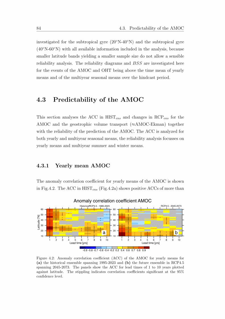
84 4.3. Predictability of the AMOC
investigated for the subtropical gyre (20�N-40�N) and the subtropical gyre
(40�N-60�N) with all available information included in the analysis, because
smaller latitude bands yielding a smaller sample size do not allow a sensible
reliability analysis. The reliability diagrams and BSS are investigated here
for the events of the AMOC and OHT being above the time mean of yearly
means and of the multiyear seasonal means over the hindcast period.
4.3 Predictability of the AMOC
This section analyses the ACC in HISTens and changes in RCPens for the
AMOC and the geostrophic volume transport (⇡AMOC-Ekman) together
with the reliability of the prediction of the AMOC. The ACC is analyzed for
both yearly and multiyear seasonal means, the reliability analysis focusses on
yearly means and multiyear summer and winter means.
4.3.1 Yearly mean AMOC
The anomaly correlation coe�cient for yearly means of the AMOC is shown
in Fig.4.2. The ACC in HISTens (Fig.4.2a) shows positive ACCs of more than
Anomaly correlation coefficient AMOC
Latit
ude
[°N]
a b
Figure 4.2: Anomaly correlation coe�cient (ACC) of the AMOC for yearly means for(a) the historical ensemble spanning 1995-2023 and (b) the future ensemble in RCP4.5spanning 2045-2073. The panels show the ACC for lead times of 1 to 10 years plottedagainst latitude. The stippling indicates correlation coe�cients significant at the 95%confidence level.
4. Potential predictability in the present and future climate 85
0.8 in the subtropical and subpolar gyre in the first lead year. For longer lead
times, the AMOC shows skill in the subtropical gyre between about 20�N and
30�N with significant predictable lead times mostly limited to about 4 years
and in the subpolar gyre with significant predictable lead times of 1-4 years,
where predictable lead times of 4 years only show up at some specific lati-
tudes. Bootstrapping gives a significance level of about 0.4. Significant ACCs
are shown with stippling in Fig.4.2 and subsequently. Around 25�N, signifi-
cant predictable lead times of up to 10 years occur. In lead year 7, the ACC
of the AMOC shows a re-emergence of skill in the subtropical gyre with sig-
nificant correlations for lead times up to ten years north of about 25�N and
in the tropical Atlantic. But a clear reason of re-emergence of skill in the
experiment has not yet been found and would need further analysis.
The ACC in RCPens (Fig.4.2b) shows prominent changes at the latitudes
with predictability in HISTens. The ACC in the first lead year drops to val-
ues of less then 0.4 at some latitudes, which have shown ACCs larger than
0.8 in HISTens. In both, the subtropical and subpolar gyre, significant pre-
dictable lead times are limited to two years in RCPens. The tropical NA in
contrast shows increased significant predictable lead times of up to 9 years
with increased ACCs in RCPens. Overall, the skill of the AMOC in HISTens
is significantly reduced and mostly lost in the subtropical and the subpolar
gyre after the second lead year .
However, it is unclear whether the prediction of the AMOC is reliable in the
model and how the reliability of the prediction changes in RCPens, whether
the changes in ACC are related to specific seasons and how the AMOC’s
geostrophic transport contributes to the changes in the ACC. To further
shed light on the changes in the predictability of the AMOC, reliability dia-
grams and the BSS for yearly means, the ACC for seasonal means (winter
spring, summer and autumn), reliability diagrams and the BSS for winter
and summer means of the AMOC, and the ACC for the geostrophic transport
are analyzed in the following.
Reliability diagrams for the AMOC for lead years 1, 2-3 and 4-5 are shown
in Fig.4.3 for the subtropical gyre (20�N-40�N) and the subpolar gyre (40�N-
60�N). The analysis of reliability for smaller latitude ranges is not feasible for
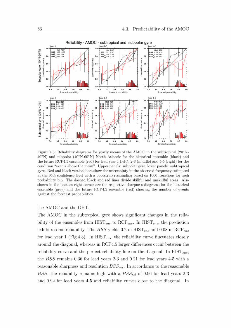
86 4.3. Predictability of the AMOC
Subpola
r gyre
(40°N
-60°N
)S
ubtr
opic
al gyre
(20°N
-40°N
)
Reliability - AMOC - subtropical and subpolar gyre
Hist RCP
BSS 0.2 0.08
BSSrel
0.96 0.85
BSSres
0.24 0.23
Hist RCP
BSS 0.36 -0.11
BSSrel
0.96 0.79
BSSres
0.41 0.09
Hist RCP
BSS 0.21 -0.09
BSSrel
0.92 0.83
BSSres
0.31 0.07
Hist RCP
BSS 0.05 -0.07
BSSrel
0.93 0.88
BSSres
0.13 0.06
Hist RCP
BSS 0.2 0.07
BSSrel
0.95 0.93
BSSres
0.25 0.13
Hist RCP
BSS 0.26 -0.11
BSSrel
0.95 0.82
BSSres
0.32 0.07
Figure 4.3: Reliability diagrams for yearly means of the AMOC in the subtropical (20�N-40�N) and subpolar (40�N-60�N) North Atlantic for the historical ensemble (black) andthe future RCP4.5 ensemble (red) for lead year 1 (left), 2-3 (middle) and 4-5 (right) for thecondition “events above the mean”. Upper panels: subpolar gyre, lower panels: subtropicalgyre. Red and black vertical bars show the uncertainty in the observed frequency estimatedat the 95% confidence level with a bootstrap resampling based on 1000 iterations for eachprobability bin. The dashed black and red lines divide skillful and unskillful areas. Alsoshown in the bottom right corner are the respective sharpness diagrams for the historicalensemble (grey) and the future RCP4.5 ensemble (red) showing the number of eventsagainst the forecast probabilities.
the AMOC and the OHT.
The AMOC in the subtropical gyre shows significant changes in the relia-
bility of the ensembles from HISTens to RCPens. In HISTens, the prediction
exhibits some reliability. The BSS yields 0.2 in HISTens and 0.08 in RCPens
for lead year 1 (Fig.4.3). In HISTens, the reliability curve fluctuates closely
around the diagonal, whereas in RCP4.5 larger di↵erences occur between the
reliability curve and the perfect reliability line on the diagonal. In HISTens,
the BSS remains 0.36 for lead years 2-3 and 0.21 for lead years 4-5 with a
reasonable sharpness and resolution BSSres. In accordance to the reasonable
BSS, the reliability remains high with a BSSrel of 0.96 for lead years 2-3
and 0.92 for lead years 4-5 and reliability curves close to the diagonal. In
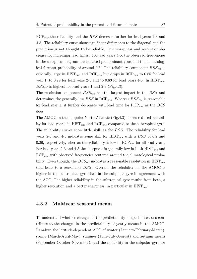
4. Potential predictability in the present and future climate 87
RCPens the reliability and the BSS decrease further for lead years 2-3 and
4-5. The reliability curve show significant di↵erences to the diagonal and the
prediction is not thought to be reliable. The sharpness and resolution de-
crease for increasing lead times. For lead years 4-5, the observed frequencies
in the sharpness diagram are centered predominantly around the climatolog-
ical forecast probability of around 0.5. The reliability component BSSrel is
generally large in HISTens and RCPens but drops in RCPens to 0.85 for lead
year 1, to 0.79 for lead years 2-3 and to 0.83 for lead years 4-5. In HISTens,
BSSrel is highest for lead years 1 and 2-3 (Fig.4.3).
The resolution component BSSres has the largest impact in the BSS and
determines the generally low BSS in RCPens. Whereas BSSres is reasonable
for lead year 1, it further decreases with lead time for RCPens as the BSS
does.
The AMOC in the subpolar North Atlantic (Fig.4.3) shows reduced reliabil-
ity for lead year 1 in HISTens and RCPens compared to the subtropical gyre.
The reliability curves show little skill, as the BSS. The reliability for lead
years 2-3 and 4-5 indicates some skill for HISTens with a BSS of 0.2 and
0.26, respectively, whereas the reliability is low in RCPens for all lead years.
For lead years 2-3 and 4-5 the sharpness is generally low in both HISTens and
RCPens with observed frequencies centered around the climatological proba-
bility. Even though, the BSSrel indicates a reasonable resolution in HISTens
that leads to a reasonable BSS. Overall, the reliability for the AMOC is
higher in the subtropical gyre than in the subpolar gyre in agreement with
the ACC. The higher reliability in the subtropical gyre results from both, a
higher resolution and a better sharpness, in particular in HISTens.
4.3.2 Multiyear seasonal means
To understand whether changes in the predictability of specific seasons con-
tribute to the changes in the predictability of yearly means in the AMOC,
I analyze the latitude-dependent ACC of winter (January-February-March),
spring (March-April-May), summer (June-July-August) and autumn means
(September-October-November), and the reliability in the subpolar gyre for
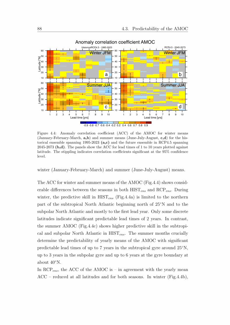
88 4.3. Predictability of the AMOC
Anomaly correlation coefficient AMOC
Winter JFM Winter JFM
Latit
ude
[°N]
Latit
ude
[°N]
Summer JJA Summer JJA
a
c
b
d
Figure 4.4: Anomaly correlation coe�cient (ACC) of the AMOC for winter means(January-February-March, a,b) and summer means (June-July-August, c,d) for the his-torical ensemble spanning 1995-2023 (a,c) and the future ensemble in RCP4.5 spanning2045-2073 (b,d). The panels show the ACC for lead times of 1 to 10 years plotted againstlatitude. The stippling indicates correlation coe�cients significant at the 95% confidencelevel.
winter (January-February-March) and summer (June-July-August) means.
The ACC for winter and summer means of the AMOC (Fig.4.4) shows consid-
erable di↵erences between the seasons in both HISTens and RCPens. During
winter, the predictive skill in HISTens (Fig.4.4a) is limited to the northern
part of the subtropical North Atlantic beginning north of 25�N and to the
subpolar North Atlantic and mostly to the first lead year. Only some discrete
latitudes indicate significant predictable lead times of 2 years. In contrast,
the summer AMOC (Fig.4.4c) shows higher predictive skill in the subtropi-
cal and subpolar North Atlantic in HISTens. The summer months crucially
determine the predictability of yearly means of the AMOC with significant
predictable lead times of up to 7 years in the subtropical gyre around 25�N,
up to 3 years in the subpolar gyre and up to 6 years at the gyre boundary at
about 40�N.
In RCPens, the ACC of the AMOC is – in agreement with the yearly mean
ACC – reduced at all latitudes and for both seasons. In winter (Fig.4.4b),
4. Potential predictability in the present and future climate 89
Anomaly correlation coefficient AMOCLa
titud
e [°N
]La
titud
e [°N
]
Spring MAM Spring MAM
Autumn SON Autumn SON
a
c
b
d
Figure 4.5: Anomaly correlation coe�cient (ACC) of the AMOC for spring means (March-April-May, a,b) and autumn means (September-October-November, c,d) for the historicalensemble spanning 1995-2023 (a,c) and the future ensemble in RCP4.5 spanning 2045-2073(b,d). The panels show the ACC for lead times of 1 to 10 years plotted against latitude.The stippling indicates correlation coe�cients significant at the 95% confidence level.
only some specific latitudes show predictability in the first lead year, but
overall no predictability is found in the whole North Atlantic. For summer
means (Fig.4.4d), there is some predictability in the subtropical gyre for lead
year 1, but beyond that no predictability is found in the ACC. In the sub-
polar gyre, the ACC of the AMOC is slightly higher than in the subtropical
gyre and significant predictable lead times extend to 2 years for summer
means. Considering the ACC for the spring (March-April-May) and autumn
(September-October-November) AMOC (Fig.4.5) shows a similar decrease
in the ACC in the subtropical and subpolar North Atlantic from HISTens to
RCPens and a predictability limited to one to two lead years for both seasons.
Obviously, the tropics also indicate an increased predictability for seasonal
means in RCPens, which is also lower than for yearly means.
Overall, all individual seasons show a lower ACC than the yearly mean
AMOC, but the ACC of the AMOC summer means represent the latitudinal
dependence of the ACC of yearly means of the AMOC to a large degree.
The highest skill in the ACC in RCPens is found for summer means in the
subpolar gyre. Therefore, the reliability of the seasonal means is analyzed for
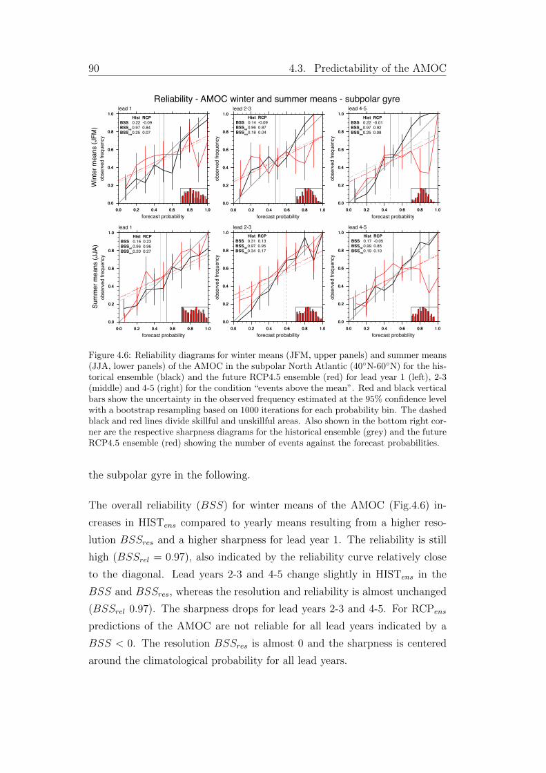
90 4.3. Predictability of the AMOC
Reliability - AMOC winter and summer means - subpolar gyreW
inte
r m
eans (
JF
M)
Sum
mer
means (
JJA
)
Hist RCP
BSS 0.22 -0.09
BSSrel
0.97 0.84
BSSres
0.25 0.07
Hist RCP
BSS 0.14 -0.09
BSSrel
0.96 0.87
BSSres
0.18 0.04
Hist RCP
BSS 0.22 -0.01
BSSrel
0.97 0.92
BSSres
0.25 0.08
Hist RCP
BSS 0.16 0.23
BSSrel
0.96 0.96
BSSres
0.20 0.27
Hist RCP
BSS 0.31 0.13
BSSrel
0.97 0.95
BSSres
0.34 0.17
Hist RCP
BSS 0.17 -0.05
BSSrel
0.99 0.85
BSSres
0.19 0.10
Figure 4.6: Reliability diagrams for winter means (JFM, upper panels) and summer means(JJA, lower panels) of the AMOC in the subpolar North Atlantic (40�N-60�N) for the his-torical ensemble (black) and the future RCP4.5 ensemble (red) for lead year 1 (left), 2-3(middle) and 4-5 (right) for the condition “events above the mean”. Red and black verticalbars show the uncertainty in the observed frequency estimated at the 95% confidence levelwith a bootstrap resampling based on 1000 iterations for each probability bin. The dashedblack and red lines divide skillful and unskillful areas. Also shown in the bottom right cor-ner are the respective sharpness diagrams for the historical ensemble (grey) and the futureRCP4.5 ensemble (red) showing the number of events against the forecast probabilities.
the subpolar gyre in the following.
The overall reliability (BSS) for winter means of the AMOC (Fig.4.6) in-
creases in HISTens compared to yearly means resulting from a higher reso-
lution BSSres and a higher sharpness for lead year 1. The reliability is still
high (BSSrel = 0.97), also indicated by the reliability curve relatively close
to the diagonal. Lead years 2-3 and 4-5 change slightly in HISTens in the
BSS and BSSres, whereas the resolution and reliability is almost unchanged
(BSSrel 0.97). The sharpness drops for lead years 2-3 and 4-5. For RCPens
predictions of the AMOC are not reliable for all lead years indicated by a
BSS < 0. The resolution BSSres is almost 0 and the sharpness is centered
around the climatological probability for all lead years.
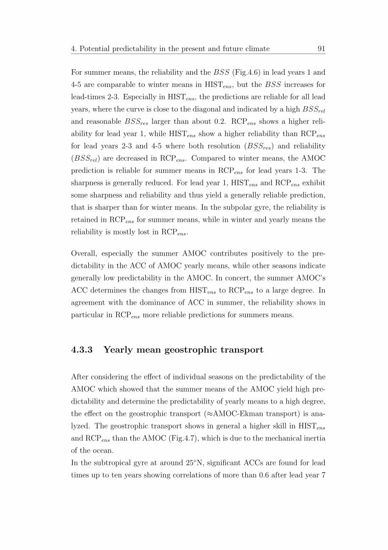
4. Potential predictability in the present and future climate 91
For summer means, the reliability and the BSS (Fig.4.6) in lead years 1 and
4-5 are comparable to winter means in HISTens, but the BSS increases for
lead-times 2-3. Especially in HISTens, the predictions are reliable for all lead
years, where the curve is close to the diagonal and indicated by a high BSSrel
and reasonable BSSres larger than about 0.2. RCPens shows a higher reli-
ability for lead year 1, while HISTens show a higher reliability than RCPens
for lead years 2-3 and 4-5 where both resolution (BSSres) and reliability
(BSSrel) are decreased in RCPens. Compared to winter means, the AMOC
prediction is reliable for summer means in RCPens for lead years 1-3. The
sharpness is generally reduced. For lead year 1, HISTens and RCPens exhibit
some sharpness and reliability and thus yield a generally reliable prediction,
that is sharper than for winter means. In the subpolar gyre, the reliability is
retained in RCPens for summer means, while in winter and yearly means the
reliability is mostly lost in RCPens.
Overall, especially the summer AMOC contributes positively to the pre-
dictability in the ACC of AMOC yearly means, while other seasons indicate
generally low predictability in the AMOC. In concert, the summer AMOC’s
ACC determines the changes from HISTens to RCPens to a large degree. In
agreement with the dominance of ACC in summer, the reliability shows in
particular in RCPens more reliable predictions for summers means.
4.3.3 Yearly mean geostrophic transport
After considering the e↵ect of individual seasons on the predictability of the
AMOC which showed that the summer means of the AMOC yield high pre-
dictability and determine the predictability of yearly means to a high degree,
the e↵ect on the geostrophic transport (⇡AMOC-Ekman transport) is ana-
lyzed. The geostrophic transport shows in general a higher skill in HISTens
and RCPens than the AMOC (Fig.4.7), which is due to the mechanical inertia
of the ocean.
In the subtropical gyre at around 25�N, significant ACCs are found for lead
times up to ten years showing correlations of more than 0.6 after lead year 7
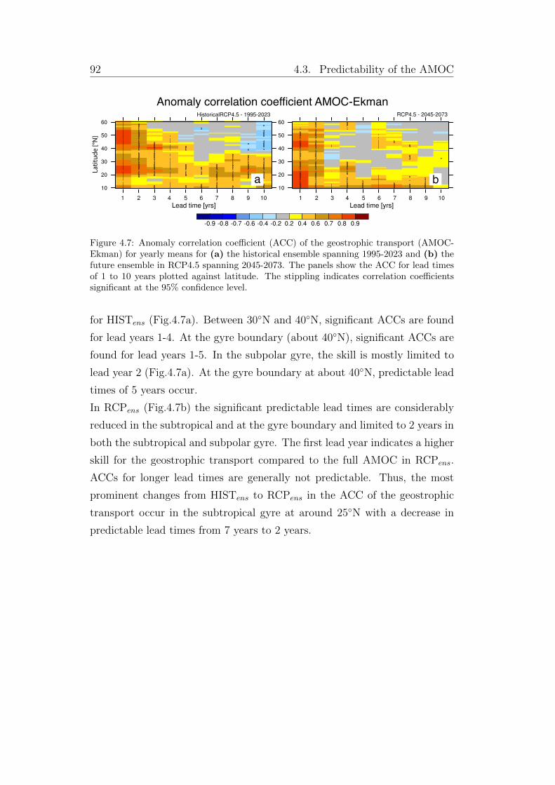
92 4.3. Predictability of the AMOC
Anomaly correlation coefficient AMOC-EkmanLa
titud
e [°N
]
a b
Figure 4.7: Anomaly correlation coe�cient (ACC) of the geostrophic transport (AMOC-Ekman) for yearly means for (a) the historical ensemble spanning 1995-2023 and (b) thefuture ensemble in RCP4.5 spanning 2045-2073. The panels show the ACC for lead timesof 1 to 10 years plotted against latitude. The stippling indicates correlation coe�cientssignificant at the 95% confidence level.
for HISTens (Fig.4.7a). Between 30�N and 40�N, significant ACCs are found
for lead years 1-4. At the gyre boundary (about 40�N), significant ACCs are
found for lead years 1-5. In the subpolar gyre, the skill is mostly limited to
lead year 2 (Fig.4.7a). At the gyre boundary at about 40�N, predictable lead
times of 5 years occur.
In RCPens (Fig.4.7b) the significant predictable lead times are considerably
reduced in the subtropical and at the gyre boundary and limited to 2 years in
both the subtropical and subpolar gyre. The first lead year indicates a higher
skill for the geostrophic transport compared to the full AMOC in RCPens.
ACCs for longer lead times are generally not predictable. Thus, the most
prominent changes from HISTens to RCPens in the ACC of the geostrophic
transport occur in the subtropical gyre at around 25�N with a decrease in
predictable lead times from 7 years to 2 years.
4. Potential predictability in the present and future climate 93
Anomaly correlation coefficient AMOC-EkmanLa
titud
e [°N
]La
titud
e [°N
]
Winter JFM Winter JFM
Summer JJA Summer JJA
a
c
b
d
Figure 4.8: Anomaly correlation coe�cient (ACC) of the geostrophic transport (AMOC-Ekman) for winter means (January-February-March, a,b) and summer means (June-July-August, c,d) for the historical ensemble spanning 1995-2023 (a,c) and the future ensemblein RCP4.5 spanning 2045-2073 (b,d). The panels show the ACC for lead times of 1 to 10years plotted against latitude. The stippling indicates correlation coe�cients significantat the 95% confidence level.
4.3.4 Multiyear seasonal means of the geostrophic
transport
Similar to the AMOC, the predictability of the geostrophic transport based on
yearly means is determined by the high predictability of the summer months
(Fig.4.8,4.9). In winter, the ACC in HISTens is limited to the subpolar gyre
and to lead years 1-2 (Fig.4.8). In contrast, the ACC of summer means
indicates skill in the subtropical and subpolar gyre with significant predictable
lead times up to 7 years at about 25�N, up to 4 years between 30�N and 40�N
and 2-3 years in the subpolar gyre.
In RCPens the predictability is reduced compared to HISTmean (Fig.4.8).
While the ACC in winter exhibits no skill in the subtropical and subpolar
gyre, the ACC in summer shows predictable lead times of 2 years in the
subpolar gyre and 1 year in the subtropical gyre, but no skill beyond.
The spring and autumn ACC of the geostrophic transport reveals (Fig.4.9)
that especially the spring also contributes considerably to the ACC of the
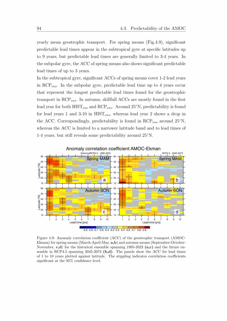
94 4.3. Predictability of the AMOC
yearly mean geostrophic transport. For spring means (Fig.4.9), significant
predictable lead times appear in the subtropical gyre at specific latitudes up
to 9 years, but predictable lead times are generally limited to 3-4 years. In
the subpolar gyre, the ACC of spring means also shows significant predictable
lead times of up to 3 years.
In the subtropical gyre, significant ACCs of spring means cover 1-2 lead years
in RCPens. In the subpolar gyre, predictable lead time up to 4 years occur
that represent the longest predictable lead times found for the geostrophic
transport in RCPens. In autumn, skillfull ACCs are mostly found in the first
lead year for both HISTens and RCPens. Around 25�N, predictability is found
for lead years 1 and 3-10 in HISTens, whereas lead year 2 shows a drop in
the ACC. Correspondingly, predictability is found in RCPens around 25�N,
whereas the ACC is limited to a narrower latitude band and to lead times of
1-4 years, but still reveals some predictability around 25�N.
Anomaly correlation coefficient AMOC-Ekman
Latit
ude
[°N]
Latit
ude
[°N]
Spring MAM Spring MAM
Autumn SON Autumn SON
a
c
b
d
Figure 4.9: Anomaly correlation coe�cient (ACC) of the geostrophic transport (AMOC-Ekman) for spring means (March-April-May, a,b) and autumn means (September-October-November, c,d) for the historical ensemble spanning 1995-2023 (a,c) and the future en-semble in RCP4.5 spanning 2045-2073 (b,d). The panels show the ACC for lead timesof 1 to 10 years plotted against latitude. The stippling indicates correlation coe�cientssignificant at the 95% confidence level.
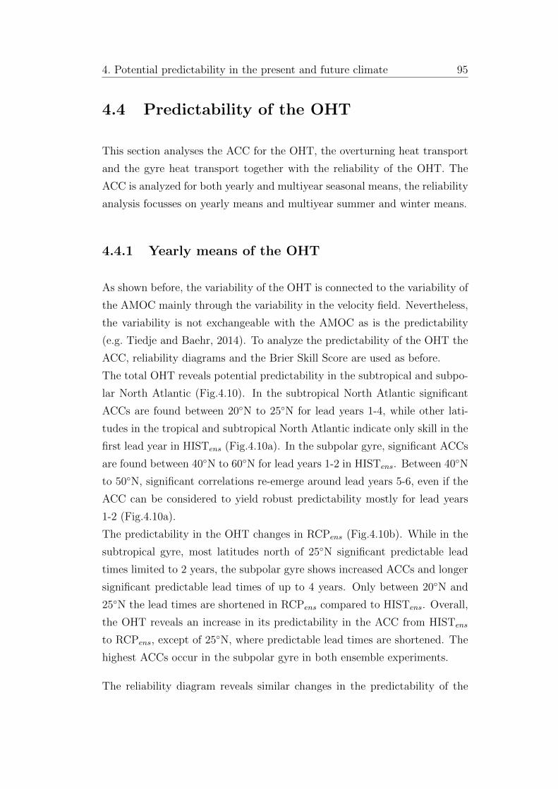
4. Potential predictability in the present and future climate 95
4.4 Predictability of the OHT
This section analyses the ACC for the OHT, the overturning heat transport
and the gyre heat transport together with the reliability of the OHT. The
ACC is analyzed for both yearly and multiyear seasonal means, the reliability
analysis focusses on yearly means and multiyear summer and winter means.
4.4.1 Yearly means of the OHT
As shown before, the variability of the OHT is connected to the variability of
the AMOC mainly through the variability in the velocity field. Nevertheless,
the variability is not exchangeable with the AMOC as is the predictability
(e.g. Tiedje and Baehr, 2014). To analyze the predictability of the OHT the
ACC, reliability diagrams and the Brier Skill Score are used as before.
The total OHT reveals potential predictability in the subtropical and subpo-
lar North Atlantic (Fig.4.10). In the subtropical North Atlantic significant
ACCs are found between 20�N to 25�N for lead years 1-4, while other lati-
tudes in the tropical and subtropical North Atlantic indicate only skill in the
first lead year in HISTens (Fig.4.10a). In the subpolar gyre, significant ACCs
are found between 40�N to 60�N for lead years 1-2 in HISTens. Between 40�N
to 50�N, significant correlations re-emerge around lead years 5-6, even if the
ACC can be considered to yield robust predictability mostly for lead years
1-2 (Fig.4.10a).
The predictability in the OHT changes in RCPens (Fig.4.10b). While in the
subtropical gyre, most latitudes north of 25�N significant predictable lead
times limited to 2 years, the subpolar gyre shows increased ACCs and longer
significant predictable lead times of up to 4 years. Only between 20�N and
25�N the lead times are shortened in RCPens compared to HISTens. Overall,
the OHT reveals an increase in its predictability in the ACC from HISTens
to RCPens, except of 25�N, where predictable lead times are shortened. The
highest ACCs occur in the subpolar gyre in both ensemble experiments.
The reliability diagram reveals similar changes in the predictability of the
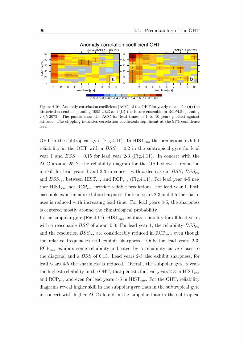
96 4.4. Predictability of the OHT
Anomaly correlation coefficient OHTLa
titud
e [°N
]
a b
Figure 4.10: Anomaly correlation coe�cient (ACC) of the OHT for yearly means for (a) thehistorical ensemble spanning 1995-2023 and (b) the future ensemble in RCP4.5 spanning2045-2073. The panels show the ACC for lead times of 1 to 10 years plotted againstlatitude. The stippling indicates correlation coe�cients significant at the 95% confidencelevel.
OHT in the subtropical gyre (Fig.4.11). In HISTens the predictions exhibit
reliability in the OHT with a BSS = 0.2 in the subtropical gyre for lead
year 1 and BSS = 0.15 for lead year 2-3 (Fig.4.11). In concert with the
ACC around 25�N, the reliability diagram for the OHT shows a reduction
in skill for lead years 1 and 2-3 in concert with a decrease in BSS, BSSrel
and BSSres between HISTens and RCPens (Fig.4.11). For lead year 4-5 nei-
ther HISTens nor RCPens provide reliable predictions. For lead year 1, both
ensemble experiments exhibit sharpness, for lead years 2-3 and 4-5 the sharp-
ness is reduced with increasing lead time. For lead years 4-5, the sharpness
is centered mostly around the climatological probability.
In the subpolar gyre (Fig.4.11), HISTens exhibits reliability for all lead years
with a reasonable BSS of about 0.3. For lead year 1, the reliability BSSrel
and the resolution BSSres are considerably reduced in RCPens, even though
the relative frequencies still exhibit sharpness. Only for lead years 2-3,
RCPens exhibits some reliability indicated by a reliability curve closer to
the diagonal and a BSS of 0.13. Lead years 2-3 also exhibit sharpness, for
lead years 4-5 the sharpness is reduced. Overall, the subpolar gyre reveals
the highest reliability in the OHT, that persists for lead years 2-3 in HISTens
and RCPens and even for lead years 4-5 in HISTens. For the OHT, reliability
diagrams reveal higher skill in the subpolar gyre than in the subtropical gyre
in concert with higher ACCs found in the subpolar than in the subtropical
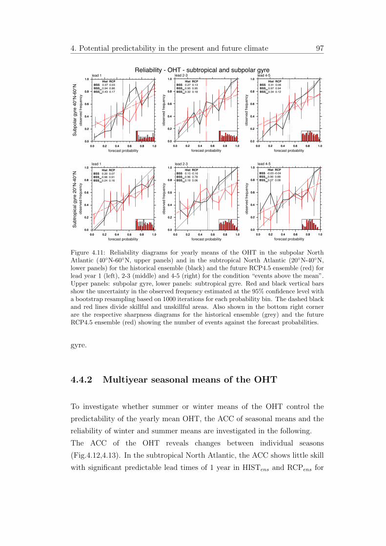
4. Potential predictability in the present and future climate 97
Hist RCP
BSS 0.20 0.07BSS
rel 0.96 0.91
BSSres
0.24 0.16
Hist RCP
BSS 0.15 -0.16BSS
rel 0.96 0.78
BSSres
0.18 0.06
Hist RCP
BSS -0.03 -0.04BSS
rel 0.90 0.88
BSSres
0.07 0.08
Hist RCP
BSS 0.31 0.06BSS
rel 0.97 0.94
BSSres
0.34 0.12
Hist RCP
BSS 0.27 0.13BSS
rel 0.95 0.95
BSSres
0.32 0.18
Hist RCP
BSS 0.37 0.03BSS
rel 0.94 0.86
BSSres
0.43 0.17
Reliability - OHT - subtropical and subpolar gyreSu
bpol
ar g
yre
40°N
-60°
NSu
btro
pica
l gyr
e 20
°N-4
0°N
Figure 4.11: Reliability diagrams for yearly means of the OHT in the subpolar NorthAtlantic (40�N-60�N, upper panels) and in the subtropical North Atlantic (20�N-40�N,lower panels) for the historical ensemble (black) and the future RCP4.5 ensemble (red) forlead year 1 (left), 2-3 (middle) and 4-5 (right) for the condition “events above the mean”.Upper panels: subpolar gyre, lower panels: subtropical gyre. Red and black vertical barsshow the uncertainty in the observed frequency estimated at the 95% confidence level witha bootstrap resampling based on 1000 iterations for each probability bin. The dashed blackand red lines divide skillful and unskillful areas. Also shown in the bottom right cornerare the respective sharpness diagrams for the historical ensemble (grey) and the futureRCP4.5 ensemble (red) showing the number of events against the forecast probabilities.
gyre.
4.4.2 Multiyear seasonal means of the OHT
To investigate whether summer or winter means of the OHT control the
predictability of the yearly mean OHT, the ACC of seasonal means and the
reliability of winter and summer means are investigated in the following.
The ACC of the OHT reveals changes between individual seasons
(Fig.4.12,4.13). In the subtropical North Atlantic, the ACC shows little skill
with significant predictable lead times of 1 year in HISTens and RCPens for
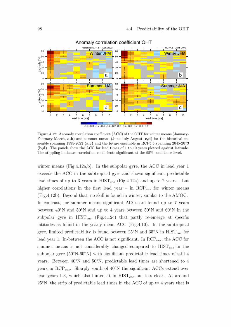
98 4.4. Predictability of the OHT
Anomaly correlation coefficient OHTLa
titud
e [°N
]La
titud
e [°N
]
Winter JFM Winter JFM
Summer JJA Summer JJA
a
c
b
d
Figure 4.12: Anomaly correlation coe�cient (ACC) of the OHT for winter means (January-February-March, a,b) and summer means (June-July-August, c,d) for the historical en-semble spanning 1995-2023 (a,c) and the future ensemble in RCP4.5 spanning 2045-2073(b,d). The panels show the ACC for lead times of 1 to 10 years plotted against latitude.The stippling indicates correlation coe�cients significant at the 95% confidence level.
winter means (Fig.4.12a,b). In the subpolar gyre, the ACC in lead year 1
exceeds the ACC in the subtropical gyre and shows significant predictable
lead times of up to 3 years in HISTens (Fig.4.12a) and up to 2 years – but
higher correlations in the first lead year – in RCPens for winter means
(Fig.4.12b). Beyond that, no skill is found in winter, similar to the AMOC.
In contrast, for summer means significant ACCs are found up to 7 years
between 40�N and 50�N and up to 4 years between 50�N and 60�N in the
subpolar gyre in HISTens (Fig.4.12c) that partly re-emerge at specific
latitudes as found in the yearly mean ACC (Fig.4.10). In the subtropical
gyre, limited predictability is found between 25�N and 35�N in HISTens for
lead year 1. In-between the ACC is not significant. In RCPens, the ACC for
summer means is not considerably changed compared to HISTens in the
subpolar gyre (50�N-60�N) with significant predictable lead times of still 4
years. Between 40�N and 50�N, predictable lead times are shortened to 4
years in RCPens. Sharply south of 40�N the significant ACCs extend over
lead years 1-3, which also hinted at in HISTens but less clear. At around
25�N, the strip of predictable lead times in the ACC of up to 4 years that is
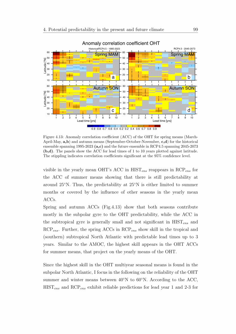
4. Potential predictability in the present and future climate 99
Anomaly correlation coefficient OHTLa
titud
e [°N
]La
titud
e [°N
]
Spring MAM Spring MAM
Autumn SON Autumn SON
a
c
b
d
Figure 4.13: Anomaly correlation coe�cient (ACC) of the OHT for spring means (March-April-May, a,b) and autumn means (September-October-November, c,d) for the historicalensemble spanning 1995-2023 (a,c) and the future ensemble in RCP4.5 spanning 2045-2073(b,d). The panels show the ACC for lead times of 1 to 10 years plotted against latitude.The stippling indicates correlation coe�cients significant at the 95% confidence level.
visible in the yearly mean OHT’s ACC in HISTens reappears in RCPens for
the ACC of summer means showing that there is still predictability at
around 25�N. Thus, the predictability at 25�N is either limited to summer
months or covered by the influence of other seasons in the yearly mean
ACCs.
Spring and autumn ACCs (Fig.4.13) show that both seasons contribute
mostly in the subpolar gyre to the OHT predictability, while the ACC in
the subtropical gyre is generally small and not significant in HISTens and
RCPens. Further, the spring ACCs in RCPens show skill in the tropical and
(southern) subtropical North Atlantic with predictable lead times up to 3
years. Similar to the AMOC, the highest skill appears in the OHT ACCs
for summer means, that project on the yearly means of the OHT.
Since the highest skill in the OHT multiyear seasonal means is found in the
subpolar North Atlantic, I focus in the following on the reliability of the OHT
summer and winter means between 40�N to 60�N. According to the ACC,
HISTens and RCPens exhibit reliable predictions for lead year 1 and 2-3 for
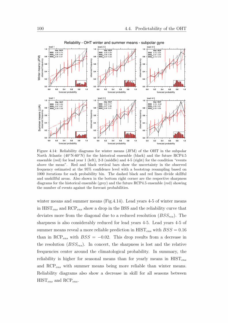
100 4.4. Predictability of the OHT
Hist RCP
BSS 0.10 0.05BSS
rel 0.97 0.94
BSSres
0.13 0.10
Hist RCP
BSS 0.20 0.20BSS
rel 0.96 0.98
BSSres
0.24 0.23
Hist RCP
BSS 0.26 0.15BSS
rel 0.96 0.94
BSSres
0.30 0.21
Hist RCP
BSS 0.32 0.35BSS
rel 0.97 0.97
BSSres
0.36 0.38
Hist RCP
BSS 0.23 0.17BSS
rel 0.97 0.96
BSSres
0.26 0.21
Hist RCP
BSS 0.16 -0.02BSS
rel 0.95 0.91
BSSres
0.20 0.06
Reliability - OHT winter and summer means - subpolar gyreW
inte
r mea
ns (J
FM)
Sum
mer
mea
ns (J
JA)
Figure 4.14: Reliability diagrams for winter means (JFM) of the OHT in the subpolarNorth Atlantic (40�N-60�N) for the historical ensemble (black) and the future RCP4.5ensemble (red) for lead year 1 (left), 2-3 (middle) and 4-5 (right) for the condition “eventsabove the mean”. Red and black vertical bars show the uncertainty in the observedfrequency estimated at the 95% confidence level with a bootstrap resampling based on1000 iterations for each probability bin. The dashed black and red lines divide skillfuland unskillful areas. Also shown in the bottom right corner are the respective sharpnessdiagrams for the historical ensemble (grey) and the future RCP4.5 ensemble (red) showingthe number of events against the forecast probabilities.
winter means and summer means (Fig.4.14). Lead years 4-5 of winter means
in HISTens and RCPens show a drop in the BSS and the reliability curve that
deviates more from the diagonal due to a reduced resolution (BSSres). The
sharpness is also considerably reduced for lead years 4-5. Lead years 4-5 of
summer means reveal a more reliable prediction in HISTens with BSS = 0.16
than in RCPens with BSS = �0.02. This drop results from a decrease in
the resolution (BSSres). In concert, the sharpness is lost and the relative
frequencies center around the climatological probability. In summary, the
reliability is higher for seasonal means than for yearly means in HISTens
and RCPens with summer means being more reliable than winter means.
Reliability diagrams also show a decrease in skill for all seasons between
HISTens and RCPens.
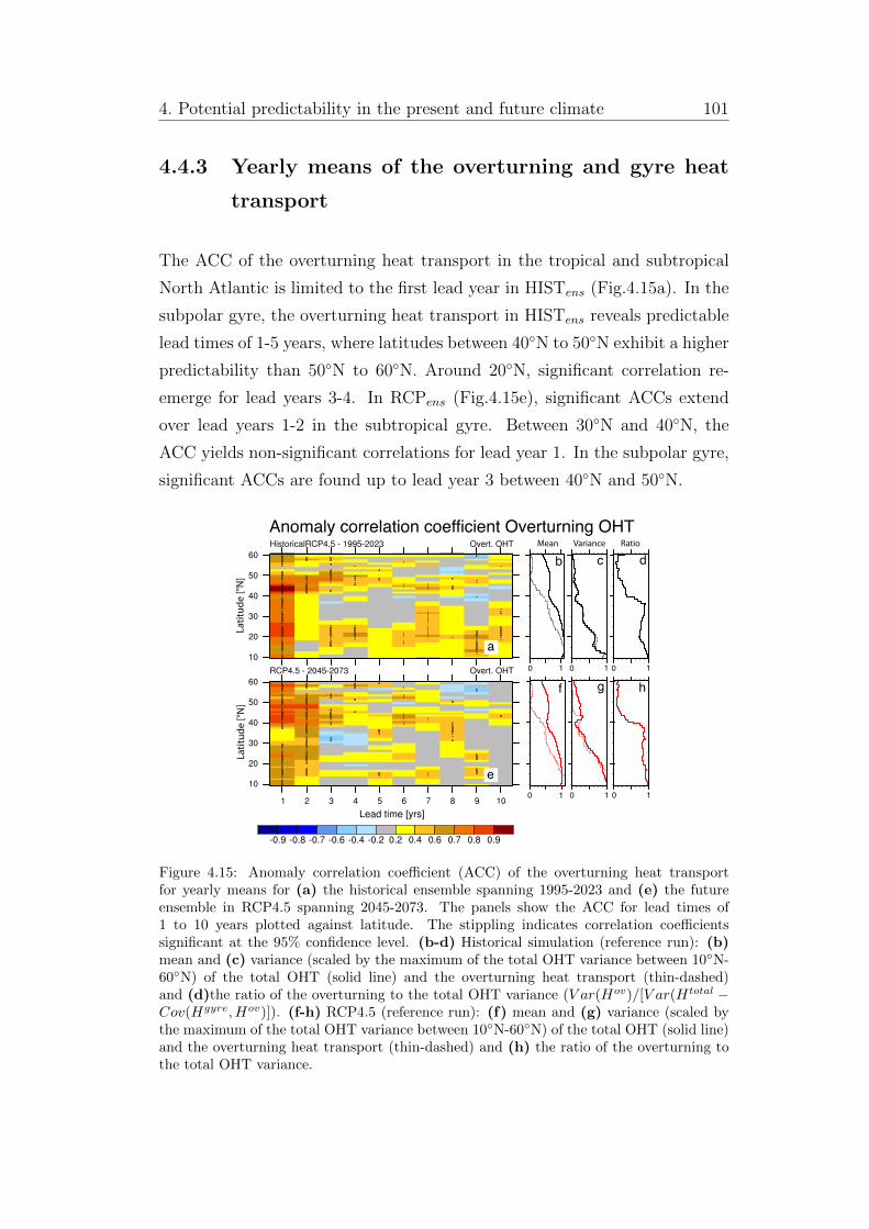
4. Potential predictability in the present and future climate 101
4.4.3 Yearly means of the overturning and gyre heat
transport
The ACC of the overturning heat transport in the tropical and subtropical
North Atlantic is limited to the first lead year in HISTens (Fig.4.15a). In the
subpolar gyre, the overturning heat transport in HISTens reveals predictable
lead times of 1-5 years, where latitudes between 40�N to 50�N exhibit a higher
predictability than 50�N to 60�N. Around 20�N, significant correlation re-
emerge for lead years 3-4. In RCPens (Fig.4.15e), significant ACCs extend
over lead years 1-2 in the subtropical gyre. Between 30�N and 40�N, the
ACC yields non-significant correlations for lead year 1. In the subpolar gyre,
significant ACCs are found up to lead year 3 between 40�N and 50�N.
Mean Variance Ratio
b c d
f g h
a
e
0 1 0 1 0 1
0 1 0 1 0 1
Anomaly correlation coefficient Overturning OHT
Latit
ude
[°N]
Latit
ude
[°N]
Figure 4.15: Anomaly correlation coe�cient (ACC) of the overturning heat transportfor yearly means for (a) the historical ensemble spanning 1995-2023 and (e) the futureensemble in RCP4.5 spanning 2045-2073. The panels show the ACC for lead times of1 to 10 years plotted against latitude. The stippling indicates correlation coe�cientssignificant at the 95% confidence level. (b-d) Historical simulation (reference run): (b)mean and (c) variance (scaled by the maximum of the total OHT variance between 10�N-60�N) of the total OHT (solid line) and the overturning heat transport (thin-dashed)and (d)the ratio of the overturning to the total OHT variance (V ar(Hov)/[V ar(Htotal �Cov(Hgyre, Hov)]). (f-h) RCP4.5 (reference run): (f) mean and (g) variance (scaled bythe maximum of the total OHT variance between 10�N-60�N) of the total OHT (solid line)and the overturning heat transport (thin-dashed) and (h) the ratio of the overturning tothe total OHT variance.
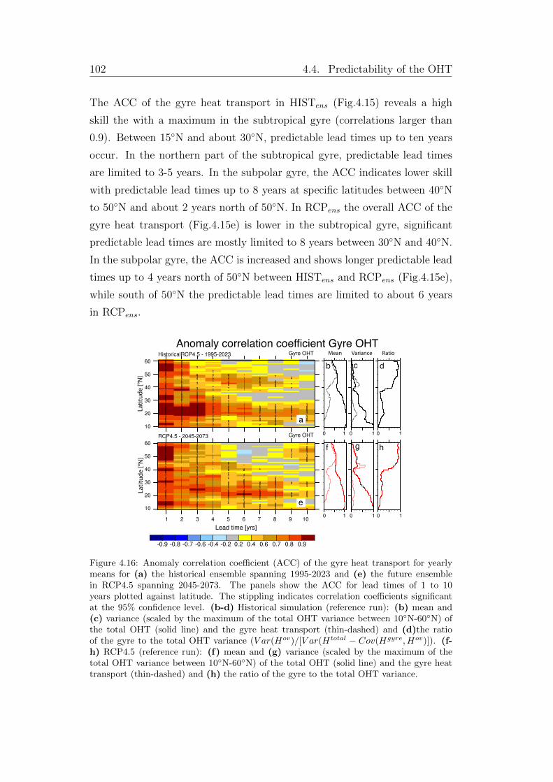
102 4.4. Predictability of the OHT
The ACC of the gyre heat transport in HISTens (Fig.4.15) reveals a high
skill the with a maximum in the subtropical gyre (correlations larger than
0.9). Between 15�N and about 30�N, predictable lead times up to ten years
occur. In the northern part of the subtropical gyre, predictable lead times
are limited to 3-5 years. In the subpolar gyre, the ACC indicates lower skill
with predictable lead times up to 8 years at specific latitudes between 40�N
to 50�N and about 2 years north of 50�N. In RCPens the overall ACC of the
gyre heat transport (Fig.4.15e) is lower in the subtropical gyre, significant
predictable lead times are mostly limited to 8 years between 30�N and 40�N.
In the subpolar gyre, the ACC is increased and shows longer predictable lead
times up to 4 years north of 50�N between HISTens and RCPens (Fig.4.15e),
while south of 50�N the predictable lead times are limited to about 6 years
in RCPens.
Mean Variance Ratio
b c d
f g h0 1 0 1 0 1
0 1 0 1 0 1
a
e
Latit
ude
[°N]
Latit
ude
[°N]
Anomaly correlation coefficient Gyre OHT
Figure 4.16: Anomaly correlation coe�cient (ACC) of the gyre heat transport for yearlymeans for (a) the historical ensemble spanning 1995-2023 and (e) the future ensemblein RCP4.5 spanning 2045-2073. The panels show the ACC for lead times of 1 to 10years plotted against latitude. The stippling indicates correlation coe�cients significantat the 95% confidence level. (b-d) Historical simulation (reference run): (b) mean and(c) variance (scaled by the maximum of the total OHT variance between 10�N-60�N) ofthe total OHT (solid line) and the gyre heat transport (thin-dashed) and (d)the ratioof the gyre to the total OHT variance (V ar(Hov)/[V ar(Htotal � Cov(Hgyre, Hov)]). (f-h) RCP4.5 (reference run): (f) mean and (g) variance (scaled by the maximum of thetotal OHT variance between 10�N-60�N) of the total OHT (solid line) and the gyre heattransport (thin-dashed) and (h) the ratio of the gyre to the total OHT variance.
4. Potential predictability in the present and future climate 103
4.4.4 Contribution of the overturning and gyre heat
transport to the predictability of the OHT
The high predictability in the ACC of the gyre heat transport compared to
the ACC of the overturning heat transport – especially in the subtropical
North Atlantic – initiates to consider the relative importance of the pre-
dictability of the gyre and overturning heat transport to the predictability of
the OHT. The overturning heat transport dominates the mean of the OHT
in the tropical and subtropical North Atlantic (Fig.4.15b, shown for the ref-
erence run), as also shown in earlier model studies (Jayne and Marotzke,
2001, Dong and Sutton, 2002). Similarly the variance in the tropical and
subtropical North Atlantic is dominated by the overturning heat transport
(Fig.4.15c,d, Fig.4.16c,d). In Fig.4.15d, the ratio of the variance of the over-
turning heat transport to the variance of the total OHT minus the covariance
of gyre and overturning heat transport (V arov/[V arOHT �Cov(gyre, ov)]) is
shown. Because the gyre and overturning heat transport are not indepen-
dent, the covariance needs to be considered for the sum of the total variance:
V arOHT = V argyre + V arov + Cov(gyre, ov).
From the high variance of the overturning heat transport compared to the
gyre heat transport in the subtropical gyre, we can expect that the pre-
dictability of the overturning component also has a higher impact on the
predictability of the total OHT. The impact of the variance can be theo-
retically understood for instance from the prognostic potential predictability
(PPP; e.g. Pohlmann et al., 2004) which gives an upper limit of potential
predictability and is in a simplified form given by:
PPP = 1� ensemble spread
variance of reference run. (4.7)
With the decomposition of the variance V arOHT as above, the PPP forms to
PPP = 1� ensemble spread
V argyre + V arov + Cov(gyre, ov). (4.8)
with the variance of the gyre heat transport V argyre, the variance of the
overturning heat transport V arov and the covariance of gyre and overturning
104 4.4. Predictability of the OHT
heat transport Cov(gyre, ov).
For latitudes with a low variance in the overturning heat transport (as in the
subpolar gyre) where the variance of the gyre heat transport dominates the
total variance (e.g. Fig.4.16c-d,g-h), the PPP yields approximately
PPP subpolar ⇡ 1� ensemble spread
V argyre + Cov(gyre, ov). (4.9)
and the PPP of the OHT is determined mostly by variance of the gyre heat
transport (assuming a low covariance).
In contrast in the subtropical gyre, where the variance of the overturning
heat transport dominates the OHT variance (e.g. Fig.4.15c-d,g-h) and is
large compared to the variance of the gyre heat transport, the PPP yields
approximately
PPP subtropical ⇡ 1� ensemble spread
V arov + Cov(gyre, ov). (4.10)
and the PPP of the OHT is determined mostly by variance of the
overturning heat transport.
This suggests, that the potential predictability from the overturning heat
transport in the subtropical gyre projects directly on the potential
predictability of the total OHT. Although PPP and ACC cannot be used
fully interchangeably, the variance suggests a similar partitioning of impact
of the ACC in the overturning and gyre heat transport on the total OHT’s
ACC. Especially in the subtropical gyre in HISTens, where the variance
of the overturning heat transport does not fully determine the variance
of the OHT (e.g. around 20�N, Fig.4.15d), there might be a reasonable
contribution of the gyre heat transport’s ACC to the OHT’s ACC. This
contribution might explain the missing skill in the ACC of the overturning
heat transport for lead years beyond one year compared to the ACC of
the full OHT. In RCPens, the overturning heat transport shows a slight
decrease in its time mean in concert with the OHT compared to HISTens
(see also chapters 2 and 3). In contrast, the variances of the OHT and the
overturning heat transport show a general increase in the tropical and
subtropical North Atlantic. At the same time, the ratio of the variance in
4. Potential predictability in the present and future climate 105
the overturning heat transport to the variance of the OHT increases in the
subtropical gyre, indicating a rise in the importance of the overturning heat
transport to the predictability of the OHT. In contrast, the variance of the
gyre heat transport dominates the variance of the OHT in the subpolar
gyre.
Following also from the PPP and assuming for simplicity a constant
ensemble spread (which is not investigated in the study), an increase in the
variance of the reference simulation would imply an increased PPP . The
increase in the variance from HISTens to RCPens in OHT in the subpolar
gyre similarly hints to an increased potential predictability. This is found
accordingly in the ACC of the OHT and the overturning heat transport in
the subtropical gyre. Both, the OHT and the overturning OHT exhibit a
more robust predictability in the subpolar gyre, with longer predictable lead
times in the OHT in RCPens. Further, an increase in predictable lead times
by one year occurs in the subtropical gyre in RCPens corresponding to an
increase in the variance in the subtropical gyre.
4.4.5 Multiyear seasonal means of the overturning and
gyre heat transport
To determine the role of seasonal means for the predictability of the
overturning and gyre heat transport, I analyze the respective ACC for
winter, spring, summer and autumn means in the following.
The overturning heat transport reveals a similar skill in the ACC of winter
means as the ACC of yearly means in HISTens (Fig.4.17a). In the
subtropical gyre, significant ACCs are limited to the first lead year, while in
the subpolar gyre ACCs extend to lead year 5 between 40�N and 50�N. The
variance (Fig.4.17c,d) shows that the overturning heat transport strongly
dominates the total variance with a ratio of almost 1 in the subtropical gyre.
In RCPens the predictability is almost lost for the ACC in the subtropical
gyre (Fig.4.17e). The subpolar gyre does not indicate considerable changes
in the ACC between HISTens to RCPens with predictable lead times of up
to 4 years between 40�N and 50�N.
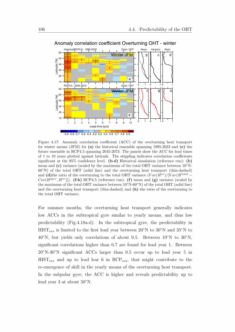
106 4.4. Predictability of the OHT
Mean Variance Ratio
b c d
f g h0 1 0 1 0 1
0 1 0 1 0 1
Anomaly correlation coefficient Overturning OHT - winter
Winter JFM
Winter JFM
a
e
Latit
ude
[°N]
Latit
ude
[°N]
Figure 4.17: Anomaly correlation coe�cient (ACC) of the overturning heat transportfor winter means (JFM) for (a) the historical ensemble spanning 1995-2023 and (e) thefuture ensemble in RCP4.5 spanning 2045-2073. The panels show the ACC for lead timesof 1 to 10 years plotted against latitude. The stippling indicates correlation coe�cientssignificant at the 95% confidence level. (b-d) Historical simulation (reference run): (b)mean and (c) variance (scaled by the maximum of the total OHT variance between 10�N-60�N) of the total OHT (solid line) and the overturning heat transport (thin-dashed)and (d)the ratio of the overturning to the total OHT variance (V ar(Hov)/[V ar(Htotal �Cov(Hgyre, Hov)]). (f-h) RCP4.5 (reference run): (f) mean and (g) variance (scaled bythe maximum of the total OHT variance between 10�N-60�N) of the total OHT (solid line)and the overturning heat transport (thin-dashed) and (h) the ratio of the overturning tothe total OHT variance.
For summer months, the overturning heat transport generally indicates
low ACCs in the subtropical gyre similar to yearly means, and thus low
predictability (Fig.4.18a-d). In the subtropical gyre, the predictability in
HISTens is limited to the first lead year between 20�N to 30�N and 35�N to
40�N, but yields only correlations of about 0.5. Between 10�N to 30�N,
significant correlations higher than 0.7 are found for lead year 1. Between
20�N-30�N significant ACCs larger than 0.5 occur up to lead year 5 in
HISTens and up to lead lear 6 in RCPens, that might contribute to the
re-emergence of skill in the yearly means of the overturning heat transport.
In the subpolar gyre, the ACC is higher and reveals predictability up to
lead year 3 at about 50�N.
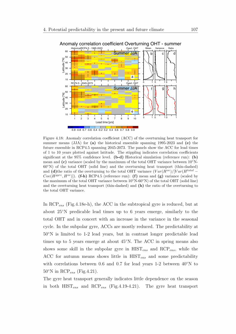
4. Potential predictability in the present and future climate 107
Mean Variance Ratio
b c d
f g h
0 1 0 1 0 1
0 1 0 1 0 1
a
e
Summer JJA
Summer JJA
Anomaly correlation coefficient Overturning OHT - summer
Latit
ude
[°N]
Latit
ude
[°N]
Figure 4.18: Anomaly correlation coe�cient (ACC) of the overturning heat transport forsummer means (JJA) for (a) the historical ensemble spanning 1995-2023 and (e) thefuture ensemble in RCP4.5 spanning 2045-2073. The panels show the ACC for lead timesof 1 to 10 years plotted against latitude. The stippling indicates correlation coe�cientssignificant at the 95% confidence level. (b-d) Historical simulation (reference run): (b)mean and (c) variance (scaled by the maximum of the total OHT variance between 10�N-60�N) of the total OHT (solid line) and the overturning heat transport (thin-dashed)and (d)the ratio of the overturning to the total OHT variance (V ar(Hov)/[V ar(Htotal �Cov(Hgyre, Hov)]). (f-h) RCP4.5 (reference run): (f) mean and (g) variance (scaled bythe maximum of the total OHT variance between 10�N-60�N) of the total OHT (solid line)and the overturning heat transport (thin-dashed) and (h) the ratio of the overturning tothe total OHT variance.
In RCPens (Fig.4.18e-h), the ACC in the subtropical gyre is reduced, but at
about 25�N predicable lead times up to 6 years emerge, similarly to the
total OHT and in concert with an increase in the variance in the seasonal
cycle. In the subpolar gyre, ACCs are mostly reduced. The predictability at
50�N is limited to 1-2 lead years, but in contrast longer predictable lead
times up to 5 years emerge at about 45�N. The ACC in spring means also
shows some skill in the subpolar gyre in HISTens and RCPens, while the
ACC for autumn means shows little in HISTens and some predictability
with correlations between 0.6 and 0.7 for lead years 1-2 between 40�N to
50�N in RCPens (Fig.4.21).
The gyre heat transport generally indicates little dependence on the season
in both HISTens and RCPens (Fig.4.19-4.21). The gyre heat transport
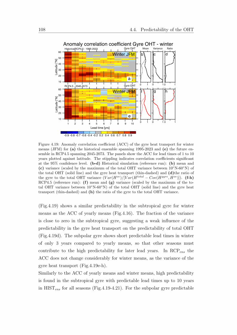
108 4.4. Predictability of the OHT
Mean Variance Ratio
b c d
f g h
0 1 0 1 0 1
0 1 0 1 0 1
a
e
Winter JFM
Winter JFM
Anomaly correlation coefficient Gyre OHT - winter
Latit
ude
[°N]
Latit
ude
[°N]
Figure 4.19: Anomaly correlation coe�cient (ACC) of the gyre heat transport for wintermeans (JFM) for (a) the historical ensemble spanning 1995-2023 and (e) the future en-semble in RCP4.5 spanning 2045-2073. The panels show the ACC for lead times of 1 to 10years plotted against latitude. The stippling indicates correlation coe�cients significantat the 95% confidence level. (b-d) Historical simulation (reference run): (b) mean and(c) variance (scaled by the maximum of the total OHT variance between 10�N-60�N) ofthe total OHT (solid line) and the gyre heat transport (thin-dashed) and (d)the ratio ofthe gyre to the total OHT variance (V ar(Hov)/[V ar(Htotal � Cov(Hgyre, Hov)]). (f-h)RCP4.5 (reference run): (f) mean and (g) variance (scaled by the maximum of the to-tal OHT variance between 10�N-60�N) of the total OHT (solid line) and the gyre heattransport (thin-dashed) and (h) the ratio of the gyre to the total OHT variance.
(Fig.4.19) shows a similar predictability in the subtropical gyre for winter
means as the ACC of yearly means (Fig.4.16). The fraction of the variance
is close to zero in the subtropical gyre, suggesting a weak influence of the
predictability in the gyre heat transport on the predictability of total OHT
(Fig.4.19d). The subpolar gyre shows short predictable lead times in winter
of only 3 years compared to yearly means, so that other seasons must
contribute to the high predictability for later lead years. In RCPens the
ACC does not change considerably for winter means, as the variance of the
gyre heat transport (Fig.4.19e-h).
Similarly to the ACC of yearly means and winter means, high predictability
is found in the subtropical gyre with predictable lead times up to 10 years
in HISTens for all seasons (Fig.4.19-4.21). For the subpolar gyre predictable
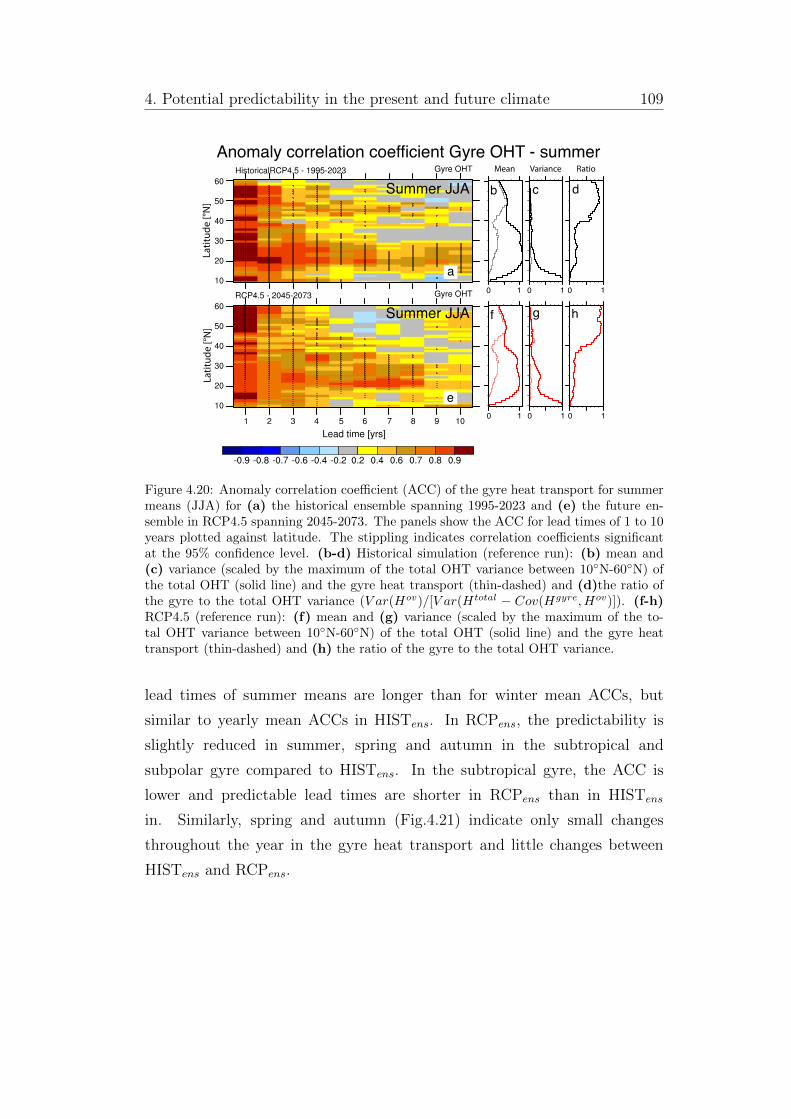
4. Potential predictability in the present and future climate 109
Mean Variance Ratio
b c d
f g h
0 1 0 1 0 1
0 1 0 1 0 1
a
e
Summer JJA
Summer JJA
Anomaly correlation coefficient Gyre OHT - summer
Latit
ude
[°N]
Latit
ude
[°N]
Figure 4.20: Anomaly correlation coe�cient (ACC) of the gyre heat transport for summermeans (JJA) for (a) the historical ensemble spanning 1995-2023 and (e) the future en-semble in RCP4.5 spanning 2045-2073. The panels show the ACC for lead times of 1 to 10years plotted against latitude. The stippling indicates correlation coe�cients significantat the 95% confidence level. (b-d) Historical simulation (reference run): (b) mean and(c) variance (scaled by the maximum of the total OHT variance between 10�N-60�N) ofthe total OHT (solid line) and the gyre heat transport (thin-dashed) and (d)the ratio ofthe gyre to the total OHT variance (V ar(Hov)/[V ar(Htotal � Cov(Hgyre, Hov)]). (f-h)RCP4.5 (reference run): (f) mean and (g) variance (scaled by the maximum of the to-tal OHT variance between 10�N-60�N) of the total OHT (solid line) and the gyre heattransport (thin-dashed) and (h) the ratio of the gyre to the total OHT variance.
lead times of summer means are longer than for winter mean ACCs, but
similar to yearly mean ACCs in HISTens. In RCPens, the predictability is
slightly reduced in summer, spring and autumn in the subtropical and
subpolar gyre compared to HISTens. In the subtropical gyre, the ACC is
lower and predictable lead times are shorter in RCPens than in HISTens
in. Similarly, spring and autumn (Fig.4.21) indicate only small changes
throughout the year in the gyre heat transport and little changes between
HISTens and RCPens.
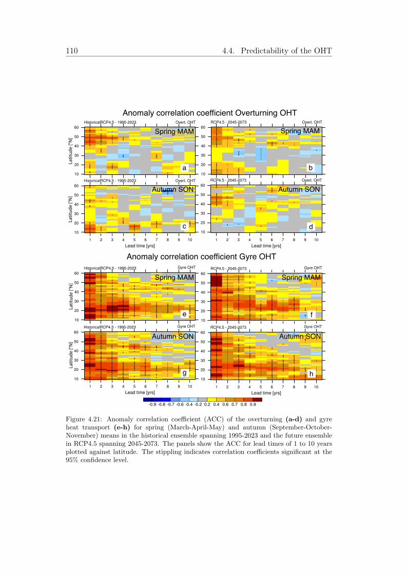
110 4.4. Predictability of the OHT
Latit
ude
[°N]
Latit
ude
[°N]
Anomaly correlation coefficient Overturning OHT
Spring MAM Spring MAM
Autumn SON Autumn SON
Spring MAM Spring MAM
Autumn SON Autumn SON
Latit
ude
[°N]
Latit
ude
[°N]
Anomaly correlation coefficient Gyre OHT
a
c
b
d
e f
g h
Figure 4.21: Anomaly correlation coe�cient (ACC) of the overturning (a-d) and gyreheat transport (e-h) for spring (March-April-May) and autumn (September-October-November) means in the historical ensemble spanning 1995-2023 and the future ensemblein RCP4.5 spanning 2045-2073. The panels show the ACC for lead times of 1 to 10 yearsplotted against latitude. The stippling indicates correlation coe�cients significant at the95% confidence level.
4. Potential predictability in the present and future climate 111
4.5 Summary and Discussion
Summary
Two ensemble hindcast experiments for a present and a future climate state in
MPI-ESM CMIP5 projections are investigated. Both, the present day ensem-
ble HISTens and the future ensemble RCPens reveal changes in the potential
predictability of the AMOC and of the OHT for the anomaly correlation co-
e�cient (ACC) and for the reliability of the predictions until the middle of
the 21st century.
(1) AMOC
For the AMOC, the predictability in the ACC and the reliability of the pre-
dictions are considerably reduced from HISTens to RCPens. The potential
predictability of the AMOC in terms of the ACC in HISTens shows pre-
dictable lead times up to 10 years in the subtropical gyre and up to 4 years in
the subpolar gyre. The structure of the predictability pattern is in agreement
with the predictability found in other studies with higher skill in the subtrop-
ical gyre than in the subpolar gyre (Tiedje et al., 2012, Bellucci et al., 2013,
Kroger et al., 2012), even if the separation of the ACCs between subtropical
and subpolar gyre is relatively sharp in HISTens and the exact patterns of
predictability di↵er between individual models (including coupled and ocean
only simulations) and based on the used initialization technique.
Reliability diagrams and the Brier Skill Score reveal that predictions of the
AMOC are overall more reliable in the subtropical gyre than in the subpolar
gyre. Between HISTens and RCPens, the reliability is considerably reduced
for yearly means and winter means. The analysis of the reliability of summer
and winter means shows, that in particular summer means yield overall more
reliable predictions in both HISTens and RCPens.
As also found in earlier studies (e.g., Matei et al., 2012a, Tiedje and Baehr,
2014), the AMOC’s predictability is determined by the geostrophic transport
112 4.5. Summary and Discussion
yielding long predictable lead times of up to 10 years in the subtropical gyre
and up to 5 years in the subpolar gyre for the present climate state. The
predictability of the AMOC and the geostrophic transport is dominated by
the considerable predictability of summer means, while the geostrophic trans-
port is additionally influenced by the predictability of spring means in the
subtropical and subpolar gyre.
For the future climate state in RCPens, the long predictability of the AMOC
and geostrophic transport is mostly lost and limited to about 2 years lead
time at all latitudes in the North Atlantic. Considering seasonal means in
RCPens, summer means reveal the strongest influence on changes in the pre-
dictability, while other seasons show an overall low predictability. The longest
predictable lead times in the geostrophic transport of 4 years occur for spring
means in the subpolar gyre for RCPens.
(2) OHT
The OHT shows a general increase in predictable lead times from HISTens
to RCPens in the ACC in both the subtropical and subpolar gyre even
though the reliability is reduced from HISTens to RCPens. The reliability of
predictions of the OHT indicates higher skill in the subpolar gyre, with
HISTens showing higher predictability than RCPens. The reliability is in
total higher for seasonal means of the OHT than for yearly means, with a
reasonable sharpness for lead years 1 and 2-3. The ACC indicates generally
higher predictability for yearly means, while amongst the multiyear seasonal
means summer means dominate the predictability in the subtropical gyre
and summer, winter and spring means contribute to predictability in the
subpolar gyre.
The gyre heat transport shows particularly high skill in the subtropical gyre
for all seasons and for both ensemble experiments HISTens and RCPens.
The predictability in the subpolar gyre is lower, but still all seasons exhibit
significant ACCs up to 7 lead years, except of the winter means where
significant ACCs are limited to 3 lead years. In the subpolar gyre, the ACC
of the gyre heat transport can largely explain the predictability in the OHT
4. Potential predictability in the present and future climate 113
and changes from HISTens to RCPens. The overturning heat transport
generally indicates lower skill than the gyre heat transport, but explains the
changes in the predictability in the subtropical gyre.
The variance of the overturning and gyre heat transport indicates that the
variability in the total OHT is dominated by the gyre heat transport in the
subpolar gyre in all seasons, while the variability in the subtropical gyre is
dominated by the overturning heat transport. Transferring changes in the
variance on the predictability by means of the PPP shows that regions with
increased variance in RCPens compared to HISTens generally indicate longer
predictable lead times, while regions with decreased variance in RCPens
compared to HISTens indicate shorter predictable lead times in the ACC.
Similar to the AMOC, the OHT reveals comparable patterns of skill in the
subtropical and subpolar gyre, although the predictive skill of the OHT in
HISTens is generally lower e.g. than for Tiedje et al. (2012). Likewise,
the overturning heat transport indicates lower skill limited to 1 year of
predictable lead time. In contrast, the gyre heat transport reveals
surprisingly high skill in HISTens compared to Tiedje et al. (2012).
Discussion
The changes in the potential predictability of the AMOC and the OHT be-
tween the present climate state represented by HISTens and a future climate
state represented by RCPens reveal changes in the overall predictability with
shortened predictable lead times and at specific latitudes with a significant
reduction in the predictable lead times and the anomaly correlation coe�-
cient. The most prominent changes occur at latitudes where considerable
changes in the seasonal cycle have been found in chapter 3.
The most significant changes in the predictability have been expected from
chapter 3 at about 25�N, between 30�N and 40�N in the subtropical gyre and
around 50�N in the subpolar gyre for the the AMOC and at 25�N, 30�N to
40�N in the subtropical gyre and between 40�N and 60�N in the subpolar
114 4.5. Summary and Discussion
gyre for the OHT. The AMOC indicates exactly at these latitudes prominent
changes in the ACCs from HISTens to RCPens, with a decrease in predictable
lead times around 25�N and around 50�N, as well as a decrease in significant
ACCs between 35�N and 40�N for lead year 1.
Similarly, the skill in the ACC is reduced for the OHT around 25�N from
HISTens to RCPens and for lead year 1 between 30�N and 40�N. These changes
result mostly from the overturning heat transport and are comparable to
the ACC of the AMOC, suggesting a relation between AMOC and OHT
predictability found in Tiedje and Baehr (2014) and similar mechanisms in-
volved. In the subpolar gyre (40�N-60�N) where the peak-to-peak amplitude
of the seasonal cycle is enhanced in the gyre heat transport in RCP4.5 and
the variance of the OHT increases in RCPens, predictable lead times are ex-
tended from about 2 years to about 4 years in the OHT.
At these specific latitude bands, changes in the peak-to-peak amplitude oc-
cur, including changes in the variance of the seasonal cycle. The changes in
the variance of the seasonal cycle contribute to changes in the total variance
especially at these latitudes jointly with the overall changes in the variance
found for the OHT, the overturning heat transport and the gyre heat trans-
port. A more detailed analysis of the variance will be needed to clearly
understand the impact of changes in the variance of the seasonal cycle on
the predictability. Nevertheless, strong hints are given by the agreement of
latitude bands that in particular the seasonal cycle peak-to-peak amplitude
(and thus the variance) impacts the potential predictability of the AMOC
and the OHT on inter-annual to decadal timescales.
For the the first time, the potential predictability of the AMOC and OHT
is analyzed for yearly means together with multiyear seasonal means. The
ACC of seasonal means is overall lower than the ACC of yearly means as also
found for temperatures before (MacLeod et al., 2012). The predictability in
the ACC for the AMOC results predominately from summer means, the pre-
dictability for the geostrophic transport results predominantly from summer
and spring means. All seasons show an overall decrease in skill from HISTens
to RCPens in the AMOC and the geostrophic transport in concert with yearly
means. The OHT similarly indicates a generally higher predictability and
4. Potential predictability in the present and future climate 115
longer predictable lead times for summer means, whereas high correlations
are found in the first lead year for winter means. The first lead year of winter
means generally indicates skillful ACCs which are thought to result from skill
in the prediction of the wind for the first months after initialization.
Changes in the seasonal cycle emerge especially around 25�N, where a shift of
the seasonal minimum and maximum of about 5 months is found in chapter
3. Significant predictable lead times of 4 years are found for yearly means of
the total OHT in HISTens, but disappear for yearly means in RCPens. This
pattern is not apparent in seasonal means in HISTens, but appears again for
summer means in RCPens. A shift in the seasons of about half a year would
suggest that in HISTens this pattern might appear for winter means, but
could be blocked by the low skill in predicting winter, spring and autumn
means. The predominance of potential predictability (in terms of the ACC)
in summer and the overall lower skill for other seasons generally restricts
conclusions concerning changes in the phase of the seasonal cycle on changes
in the potential predictability of specific seasons.
Regarding the question whether the decadal predictions have su�cient reli-
ability to provide useful information to users the reliability and Brier Skill
Score has been analyzed for the AMOC and OHT for the first time here.
Corti et al. (2012) have shown, that predictions of surface temperatures over
the North Atlantic might exhibit some reliability. Here, I have shown, the
HISTens indicates some reliability for the AMOC up to lead year 3 that is
higher in the subtropical gyre, even after a linear trend is removed. The
reliability of the AMOC in RCPens is generally low so that the predictions
cannot be considered reliable. The reliability for winter and summer means
of the AMOC providing reliable predictions up to lead year 5 is comparable
in HISTens to yearly means. In RCPens predictions of winter means do not
reveal any reliability in contrast to summer means, where predictions of the
AMOC are reliable for lead year 1-3.
The OHT also exhibits some reliability in the subtropical and subpolar gyre,
whereas the reliable predictions are limited to HISTens for lead years 1-3. The
reliability of OHT predictions in the subpolar is generally higher and also in-
dicates some reliability in RCPens. For individual seasons, reliable forecasts
116 4.6. Conclusions
are also found in RCPens for lead years 1-3.
Overall, the reliability analysis reveals, that the skill in the AMOC is re-
duced in the subtropical and subpolar gyre from HISTens to RCPens. But,
the applicability of the reliability analysis for real predictions of the AMOC
and OHT is analogously limited as for deterministic measures (e.g, Matei
et al., 2012a, Vecchi et al., 2012), since observations of the AMOC and OHT
are still relatively short (Smeed et al., 2015) and need further decades and a
broader ranges of latitudes to allow for a sensible evaluation of the reliability
of the AMOC and the OHT.
4.6 Conclusions
Based on the analysis of the potential predictability of the AMOC and the
OHT for a present climate state in the CMIP5 historical simulation extended
with RCP4.5 (1995-2023) and a future climate state in RCP4.5 (2045-2073)
I conclude:
• The AMOC exhibits latitude-dependent potential predictability for the
present climate state in HISTens with predictable lead times up to 4
years, that decrease in the future ensemble RCPens to 2 years at all
latitudes. The skill in the anomaly correlation coe�cient results mostly
from the predictability of summer months and largely from the high skill
in predicting the geostrophic transport.
• For the present climate, the ACC of the AMOC and the OHT reveals
similar latitudes with high skill (around 25�N and 40�N to 60�N). In
contrast to the AMOC, the OHT reveals increased predictable lead
times of 4 years in the subpolar gyre in RCPens, but a consistant reduc-
tion in predictable lead times to to 2 years at 25�N in the subtropical
gyre in RCPens.
• Considerable changes in the ACC are found around 25�N and in the
subpolar gyre between 40�N to 60�N for the AMOC and the OHT from
4. Potential predictability in the present and future climate 117
HISTens to RCPens in agreement with latitudes that reveal prominent
changes in the AMOC and the OHT seasonal cycle.
• The skill in the OHT cannot be explained explicitly by either the over-
turning heat transport or the gyre heat transport. The overturning heat
transport reveals generally lower skill in the ACC, while the gyre heat
transport reveals notably high skill in the ACC in both the subtropical
and subpolar gyre and for HISTens and RCPens.
• From the variance of the gyre and overturning heat transport in HISTens
and RCPens follows that the gyre heat transport dominates the pre-
dictability and its changes in the subpolar gyre, while the overturning
heat transport dominates the predictability and its changes in the sub-
tropical gyre.
• The reliability analysis suggests changes in concert with the ACC for
the AMOC and the OHT in the subtropical and subpolar gyre. Pre-
dictions of seasonal means indicate a higher reliability than predictions
of yearly means. Generally, predictions of the OHT are more reliable
than predictions of the AMOC. For both, the AMOC and the OHT
predictions are more reliable in HISTens than in RCPens.

5 Summary and Conclusions
To investigate the e↵ect of global warming on the North Atlantic ocean circu-
lation and on the potential predictability of the Atlantic meridional overturn-
ing circulation (AMOC) and the Atlantic meridional heat transport (OHT) I
have first analyzed changes in the AMOC and OHT with a focus on their sea-
sonal cycles in the Max-Planck-Institute Earth System Model (MPI-ESM).
Subsequently, I have analyzed changes in the potential predictability of the
AMOC and the OHT between a present climate state in the Coupled Model
Intercomparison Project phase 5 (CMIP5) historical simulation (HISTens)
and a projected future climate state in RCP4.5 (RCPens) that might result
from changes in the seasonal cycle of the AMOC and the OHT.
All results are based on climate simulations with the Max-Planck-Institute
Earth System Model. The analysis of changes in the AMOC and OHT sea-
sonal cycle is based on the MPI-ESM CMIP5 climate projections with all
limitations and uncertainties inherent in climate projections (e.g., Knutti and
Sedlacek, 2013). Yet, the analysis in this thesis is performed in one single
ensemble member of the CMIP5 projections in MPI-ESM and thus ensures a
physically consistent framework for the analysis. Even though, results might
di↵er in other models contributing CMIP5.
For the predictability analysis, two ensemble experiments are performed in
MPI-ESM. Because the decadal predictability of a future climate can only
be studied in terms of potential predictability, both ensemble experiments
are based on “uninitialized” simulations from CMIP5 to ensure comparabil-
ity of the two experiments. Using the anomaly correlation coe�cient (ACC)
together with reliability diagrams and the Brier Skill Score (BSS), the ensem-
120
ble means are validated against the same respective CMIP5 simulation in the
sense of a “perfect model” framework. Thus, the results of the predictability
analysis rather give an upper limit of predictability given a “perfect model
world” and near perfect knowledge of the initial conditions in the ocean and
the atmosphere that will never be achieved in the real world. Nevertheless,
the use of a coupled comprehensive climate model enables us to include ef-
fects from the ocean, atmosphere, sea ice and land into the analysis. Further,
the analysis has the advantage of a consistent experimental setup for both
(1) the analysis of changes in the seasonal variability of the AMOC and the
OHT and (2) the predictability analysis with respect to initialization and
consistency with the reference simulation.
In the following, I will summarize the main results and conclude this thesis
by answering the questions raised in the introduction.
Changes in the seasonal variability of the Atlantic meridional over-
turning circulation and the meridional heat transport in a future
climate
• What changes do emerge in the mean state of the North Atlantic ocean
circulation, the AMOC and the OHT due to global warming in the MPI-ESM
climate projections?
The North Atlantic Ocean reveals a considerable warming of sea surface
temperatures under global warming. The strongest warming occurs in
RCP8.5 until the 23rd century in polar regions and a less intense warming
in the subpolar gyre. Surface salinities reveal a freshening in the subpolar
gyre, and an increase of salinity in the subtropical gyre. This implies
changes in the North Atlantic gyre circulation which is shifted northward by
about 5 degrees in RCP8.5 in concert with a northward shift in the surface
winds (chapter 2).
Changes in the ocean circulation impact the AMOC and OHT (chapter
2). Both show considerable changes between the present climate state
in HISTens and a future climate state in RCPens. The AMOC shows a
5. Summary and Conclusions 121
weakening by about 50% in the North Atlantic in RCP8.5 until the
23rd century resulting from a weakening of the geostrophic transport
(AMOC-Ekman). The OHT shows a 30 to 50% decline in the time-mean
that results from a weakening of the overturning heat transport in the
subtropical gyre and a weakening of both, the overturning and gyre heat
transport in the subpolar gyre (section 2.1). A decomposition of the OHT
in density coordinates reveals a considerable reduction in the surface and
intermediate layers, and a further reduction in the OHT related to the
formation of the North Atlantic Deep Water (NADW) that is almost
absent in RCP8.5 in the 23rd century (section 2.1). An equivalent finding
is obtained from the OHT decomposition based on a heat function in
potential temperature coordinates (section 2.2).
For near-term changes until the middle of the 21st century, the RCP8.5
scenario in MPI-ESM indicates a global mean temperature increase by more
than 2�C and a reduction in the OHT and AMOC by 10-20% compared
to the historical simulation. Similarly, the RCP4.5 scenario indicates a
global temperature increase of almost 2�C and a reduction of the OHT and
AMOC by about 10% (chapter 3).
• Do projected changes in the mean state of the North Atlantic ocean circu-
lation imply changes in the seasonal cycle of the OHT until the end of the
23rd century in the MPI-ESM climate projections?
In concert with the decline, the OHT seasonal cycle shows shifts in time (1
to 6 months, depending on latitude and season) and space (5� northward, of
the seasonal cycle pattern) for long-term changes between the present
climate state in the historical simulation and the 23rd century in RCP8.5
(chapter 2).
The OHT seasonal cycle reveals changes in both the subtropical and
subpolar gyre. These changes stem from a latitude-dependent altered
seasonal cycle and a northward shift by about 5 degrees in the atmospheric
Hadley circulation and resulting changes in the surface winds. These lead to
a temporal shift by 1 to 5 months in the seasonal cycle of the Ekman
122
heat transport and the overturning heat transport (section 2.1). The
vertical structure of the OHT reveals that in tropical and subtropical North
Atlantic, the OHT seasonal cycle is mostly driven and mostly changed in
the surface and intermediate layers where the wind acts as the dominant
direct driver of the seasonal variability and leads to temporal shifts from
1 to 6 months. In the subpolar North Atlantic, the process of NADW
formation contributes to the seasonal cycle in the historical simulation,
while this contribution is significantly reduced in RCP8.5 until the 23rd
century due to a reduction in the NADW formation (section 2.1).
The vertical decomposition of the OHT seasonal cycle in potential
temperature coordinates (section 2.2) indicates that the mixed
(residual) circulation – that also determines the mean OHT – drives
a large fraction of changes in the OHT seasonal cycle. Further
changes occur in the wind-driven surface cell that indicates an
intensified seasonal cycle and in a cold cell related to the NADW
formation where the absent NADW formation extinguishes the seasonal cycle.
• Are changes in the seasonal cycle already noticeable in the near future in
the middle of the 21st century?
Changes in the seasonal cycle of the AMOC and the OHT already emerge
in the middle of the 21st century in RCP4.5 and RCP8.5 with latitude-
dependent temporal shifts in the seasonal cycle and changes in the seasonal
peak-to-peak amplitude (chapter 3). Between RCP4.5 and RCP8.5, changes
in the seasonal cycle show a similar dependence on latitude with slightly
larger adjustments in RCP8.5.
For the seasonal amplitude of the AMOC (chapter 3) changes occur in both
the subtropical and subpolar gyre. The largest changes occur in the subtrop-
ical gyre between 25�N and 35�N with reduction in the seasonal amplitude
and between 35�N and 50�N with an increase in the seasonal amplitude be-
tween the present climate state and the middle of the 21st century. The rest
subpolar gyre also indicates a general reduction in the seasonal amplitude.
These changes predominantly result from changes in the Ekman transport
5. Summary and Conclusions 123
seasonal cycle. Changes in the seasonal cycle of the geostrophic transport
are weaker, but also emerge in the subtropical and subpolar gyre. The min-
ima and maxima in the AMOC seasonal cycle are also shifted between the
present climate state and the middle of the 21st century, especially between
25�N and 30�N in the subtropical gyre and between 35�N and 50�N from the
subtropical to the subpolar gyre.
The seasonal cycle of the OHT (chapter 3) reveals a decreased seasonal peak-
to-peak amplitude in the subtropical gyre that results from the seasonal cycle
of the overturning heat transport, in particular between 20�N and about 30�N
and an increase in the peak-to-peak amplitude between about 30�N and 40�N.
Changes in the seasonal cycle of the gyre heat transport become important
in the subpolar gyre where the seasonal peak-to-peak amplitude is increased
at most latitudes between 35�N and 60�N in the subtropical and the subpolar
gyre between the present climate state and the middle of the 21st century.
Only around 50�N, the seasonal amplitude is considerably reduced. Overall
the OHT seasonal minima and maxima are shifted at the latitudes where the
amplitude reveals the largest shifts in the subtropical gyre. Temporal shifts
up to 5 months occur in particular between 20�N and about 30�N and about
30�N to 40�N in the subtropical gyre, and between 45�N and 55�N in the sub-
polar gyre. These latitude bands with largest shifts in the seasonal phase and
amplitude might lead to considerable changes in the potential predictability
of the AMOC and OHT (chapter 4).
The influence of the AMOC and OHT especially on the European climate
is still under discussion (e.g., Riser and Lozier, 2013). The changes in the
seasonal cycle of the AMOC and the OHT imply changes in the seasonally
dependent heat transports into the North Atlantic that might also a↵ect
the (seasonal) variability of the ocean heat content, surface temperatures
or surface heat fluxes. Via this interaction at the surface, the AMOC and
OHT (seasonal) variability is linked to the European climate, although exact
mechanism are not yet clear. Thus, the changes in the AMOC and OHT sea-
sonal cycle motivate to advance the understanding of the relation between
the North Atlantic ocean circulation and the European climate. Future re-
search might focus on the understanding of the specific role of the changes
in the seasonal cycle found in this study on potential climate impacts on the
124
European continent.
Potential predictability of the Atlantic meridional overturning cir-
culation and the Atlantic meridional heat transport
• Does the potential predictability of the AMOC and the OHT change between
the present climate state and a projected future climate state?
The potential predictability of the AMOC and OHT is found to change in a
future climate state in RCP4.5 (RCPens, chapter 4). The AMOC indicates
a latitude-dependent potential skill in the ACC for the present climate state
(HISTens) with up to 4 years. Predictable lead times in the ACC are reduced
to 2 years at all latitudes for the AMOC under global warming in RCPens.
Skillfull correlations in the AMOC are related to the geostrophic transport
that also shows a considerable decrease in predictable lead times in RCPens
compared to HISTens.
The OHT shows higher skill in the subpolar North Atlantic than in the sub-
tropical North Atlantic. In contrast to the AMOC, the OHT shows an in-
crease in predictable lead times in the subpolar gyre from 2-3 years to 4-5
years, but also a decrease in the subtropical gyre from up to 4 years in
HISTens to 2 years in RCPens. Changes in the predictability of the OHT
are dominated by the gyre heat transport in the subpolar gyre and by both
overturning heat transport and gyre heat transport in the subtropical gyre.
The reliability and Brier Skill Score of decadal predictions of the AMOC and
OHT are considerably reduced in a future climate in RCPens compared to
HISTens in the subtropical and subpolar gyre. For the OHT, this is in con-
trast to the ACC that indicates higher skill in the subpolar gyre in RCPens.
The considerable reduction in the reliability, making the prediction unreli-
able, questions whether the prediction is still potentially useful. Although
the exact reason for the loss in reliability is not studied further in this thesis,
this fact might demonstrate the need to further improve ensemble generation
techniques and methods used in decadal prediction, in particular if real world
predictability might weaken similarly.
5. Summary and Conclusions 125
• Is there an impact of changes in the seasonal cycle on the potential pre-
dictability of the AMOC and OHT and do specific latitudes show more promi-
nent changes than others?
In the subtropical gyre, latitudes of high predictability agree for ACCs of
the AMOC and the OHT in the present climate state (HISTens, chapter
4). Predictable lead times of up to 10 years in the AMOC and up to 4
years in the OHT emerge between 20�N and 30�N. In that latitude band,
correlations are reduced and predictable lead times are shortened to 2 years
in RCPens for both the AMOC and the OHT in accordance with latitudes
where prominent changes in the seasonal cycle occur and in particular the
variance of the seasonal cycle is reduced (chapter 3). This suggests that
changes in the seasonal cycle can impact the potential predictability of the
AMOC and the OHT.
In the AMOC the peak-to-peak amplitude is reduced suggesting a reduction
in the variance of the AMOC. The reduction in the variance suggests a
reduction of potential predictability. In concert, the OHT shows a decrease
in the peak-to-peak amplitude between 20�N and 30�N together with a
decrease in the variance. The ACC of the OHT is also reduced between
20�N and 30�N (chapter 4). Exactly here, the OHT indicates the largest
temporal shift in the seasonal maxima from the present climate state to a
future climate state (chapter 3), so that the reduction in ACC might be
related to a considerable temporal shift and a reduction in variance in the
OHT seasonal cycle.
In the subpolar gyre, the predictable lead times are uniformly reduced
for the AMOC following the reduction in the seasonal amplitude in the
subpolar North Atlantic. The potential predictability of the OHT is
determined by the gyre heat transport. The ACC of the gyre heat transport
shows an increase of predictable lead times in the subpolar gyre following
the overall increase in the seasonal peak-to-peak amplitude and accordingly
in the variance of the gyre heat transport at most latitudes in the subpolar
gyre. Hence, the increase in predictable lead times in the ACC of gyre heat
transport lead to increased predictable lead times in the ACC of the OHT
in the subpolar gyre.
126
Overall, the AMOC and OHT indicate latitudes with prominent
changes in the predictability. In particular between 20�N
and 30�N in the subtropical gyre, considerable changes occur
in the predictable lead times of the AMOC and the OHT
between HISTens and RCPens. These latitudes refer to latitudes
bands in the subtropical gyre with considerable changes in the seasonal cycle.
• Do changes in the seasonal cycle project onto the potential predictability of
multiyear seasonal means of the AMOC and the OHT?
For multi-year seasonal means, the potential predictability is analyzed using
the ACC and reliability diagram with the Brier Skill Score for winter and
summer means. Overall, the potential predictability of the AMOC of winter
means, spring means and autumn means is low. The potential predictability
of the yearly mean AMOC is dominated by summer means. For summer
means, the skill is reduced in RCPens compared to HISTens in the subtropical
and subpolar gyre, as for yearly means. The predominance of skill in summer
means and the low skill in the remaining seasons in ACC limit a noticeable
impact of a potential shift in the seasonal cycle on the ACC of multiyear
seasonal means. This applies in particular to the low ACCs in winter means,
spring means and autumn means, that limit a clear detection of a potential
impact of changes in the seasonal cycle.
For the OHT, the ACC of yearly means is similarly characterized by the
predictability of summer means which shows an increase in predictable lead
times in the future ensemble RCPens. Additionally, spring means yield some
predictability in the subpolar gyre in RCPens. Only summer means show
potential predictability for latitudes between 25�N and 30�N up to 5 years in
RCPens. Between 25�N and 30�N, potential predictability is also found for
yearly means in HISTens, but potential predictability is considerably reduced
for yearly means in RCPens. This reveals, that some predictability remains
between 25�N and 30�N for summer means in RCPens, although the seasonal
cycle changes notably at these latitudes.
The results demonstrate the need to foster further understanding and devel-
5. Summary and Conclusions 127
opment of techniques used in decadal prediction. With the methodologies
(ACC and reliability) used in this study and commonly used in decadal pre-
diction, skill in predicting the AMOC and OHT is mostly lost under future
climate due to changes in the variance of the yearly mean AMOC and OHT
as well as changes in the variance of the seasonal cycle at specific latitudes.
This is in agreement with conceptual studies of potential predictability (e.g.,
Boer, 2009). Whether other metrics or an improved initialization of the hind-
casts can yield more reliable predictions and a better potential predictability
under future climate conditions is unclear.
Whether this result can directly be transferred to “real world” predictability
can – of course – be questioned. But since the perfect model predictability
generally gives an upper limit of predictability, an albeit higher reduction in
predictability and predictive skill could potentially result from global warm-
ing for “real world” predictions. The results motivate to conduct further
research of changes in the potential predictability under global warming, e.g.
for relevant climate parameters that reveal a more direct connection to the
North American and European climate such as surface temperatures and heat
fluxes or precipitation and their impacts in individual seasons.

6 Bibliography
Andrews, D. G. (1983). A finite-amplitude Eliassen-Palm theorem in isen-
tropic coordinates. Journal of the Atmospheric Sciences, 40 (8), 1877–1883.
Baehr, J. and Piontek, R. (2013). Ensemble initialization of the oceanic com-
ponent of a coupled model through bred vectors at seasonal-to-interannual
time scales. Geoscientific Model Development Discussions, 6, 5189–5214.
Balan Sarojini, B., Gregory, J. M., Tailleux, R., Bigg, G. R., Blaker, A. T.,
Cameron, D. R., Edwards, N. R., Megann, A. P., Sha↵rey, L. C., and
Sinha, B. (2011). High frequency variability of the Atlantic meridional
overturning circulation. Ocean Science, 7 (4), 471–486.
Barrier, N., Cassou, C., Deshayes, J., and Treguier, A.-M. (2014). Response
of North Atlantic Ocean Circulation to Atmospheric Weather Regimes.
Journal of Physical Oceanography, 44 (1), 179–201.
Bellucci, A., Gualdi, S., Masina, S., Storto, A., Scoccimarro, E., Cagnazzo,
C., Fogli, P., Manzini, E., and Navarra, A. (2013). Decadal climate predic-
tions with a coupled OAGCM initialized with oceanic reanalyses. Climate
dynamics, 40 (5-6), 1483–1497.
Bintanja, R. and Van der Linden, E. (2013). The changing seasonal climate
in the Arctic. Scientific reports, 3.
Boccaletti, G., Ferrari, R., Adcroft, A., Ferreira, D., and Marshall, J. (2005).
The vertical structure of ocean heat transport. Geophysical Research Let-
ters, 32 (10).
130
Boer, G. (2009). Changes in interannual variability and decadal potential
predictability under global warming. Journal of Climate, 22 (11), 3098–
3109.
Boer, G. J. (2004). Long time-scale potential predictability in an ensemble
of coupled climate models. Climate Dynamics, 23 (1), 29–44.
Boning, C., Dieterich, C., Barnier, B., and Jia, Y. (2001). Seasonal cycle
of meridional heat transport in the subtropical North Atlantic: A model
intercomparison in relation to observations near 25�N. Progress in Oceanog-
raphy, 48(2), 231–253.
Boning, C. and Hermann, P. (1994). Annual cycle of poleward heat transport
in the ocean: Results from high-resolution modelling of the North and
Equatorial Atlantic. Journal of Physical Oceanography, 24(10), 91–107.
Brier, G. W. (1950). Verification of forecasts expressed in terms of probability.
Monthly weather review, 78 (1), 1–3.
Bryan, K. (1962). Measurements of meridional heat transport by ocean cur-
rents. Journal of Geophysical Research, 67 (9), 3403–3414.
Bryan, K. (1982a). Poleward heat transport by the ocean: observations and
models. Annual Review of Earth and Planetary Sciences, 10, 15.
Bryan, K. (1982b). Seasonal variation in meridional overturning and poleward
heat transport in the Atlantic and Pacific Oceans: A model study. J. Mar.
Res., 40, 39–53.
Bryan, K. and Sarmiento, J. L. (1985). Modeling ocean circulation. Advances
in geophysics, 28, 433–459.
Bryden, H. and Imawaki, S. (2001). Ocean heat transport. In G. Siedler, J.
Church, and J. Gould (Eds.), Ocean circulation and climate: observing and
modelling the global ocean, volume 77 of International Geophysics Series,
chapter 6.1, volume 77 (pp. 455–474). San Francisco: Academic Press.
Bryden, H. L. (1993). Ocean heat transport across 24�N latitude. Interactions
Between Global Climate Subsystems the Legacy of Hann, , 65–75.
6. Bibliography 131
Butler, A. H., Thompson, D. W., and Heikes, R. (2010). The Steady-
State Atmospheric Circulation Response to Climate Changelike Thermal
Forcings in a Simple General Circulation Model. Journal of Climate, 23
(13), 3474–3496.
Cabanes, C., Lee, T., and Fu, L. (2008). Mechanisms of Interannual Vari-
ations of the Meridional Overturning Circulation of the North Atlantic
Ocean. Journal of Physical Oceanography, 38(2).
Carton, J. A., Ding, Y., and Arrigo, K. R. (2015). The seasonal cycle of the
Arctic Ocean under climate change. Geophysical Research Letters, .
Chang, E. K., Guo, Y., and Xia, X. (2012). CMIP5 multimodel ensemble
projection of storm track change under global warming. Journal of Geo-
physical Research: Atmospheres (1984–2012), 117 (D23).
Cheng, W., Chiang, J., and Zhang, D. (2013). Atlantic Meridional Overturn-
ing Circulation (AMOC) in CMIP5 Models: RCP and Historical Simula-
tions. Journal of Climate, 26(18).
Chidichimo, M., Kanzow, T., Cunningham, S., Johns, W., and Marotzke,
J. (2010). The contribution of eastern-boundary density variations to the
Atlantic meridional overturning circulation at 26.5�N. Ocean Science, 6
(2), 475–490.
Christensen, J., Krishna Kumar, K., Aldrian, E., An, S.-I., Cavalcanti, I.,
de Castro, M., Dong, W., Goswami, P., Hall, A., Kanyanga, J., Kitoh, A.,
Kossin, J., Lau, N.-C., Renwick, J., Stephenson, D., S.-P., X., and Zhou,
T. (2013). Climate Phenomena and their Relevance for Future Regional
Climate Change. In T. Stocker, D. Qin, G.-K. Plattner, M. Tignor, S.
Allen, J. Boschung, A. Nauels, Y. Xia, B. V., and P. Midgley (Eds.), Cli-
mate Change 2013: The Physical Science Basis. Contribution of Working
Group I to the Fifth Assessment Report of the Intergovernmental Panel on
Climate Change. Cambridge, United Kingdom and New York, NY, USA:
Cambridge University Press.
Collins, M. (2002). Climate predictability on interannual to decadal time
scales: the initial value problem. Climate Dynamics, 19 (8), 671–692.
132
Collins, M. and Allen, M. R. (2002). Assessing the relative roles of initial
and boundary conditions in interannual to decadal climate predictability.
Journal of Climate, 15 (21), 3104–3109.
Collins, M., Botzet, M., Carril, A., Drange, H., Jouzeau, A., Latif, M.,
Masina, S., Otteraa, O., Pohlmann, H., Sorteberg, A., et al. (2006).
Interannual to decadal climate predictability in the North Atlantic: a
multimodel-ensemble study. Journal of climate, 19 (7), 1195–1203.
Collins, M. and Sinha, B. (2003). Predictability of decadal variations in the
thermohaline circulation and climate. Geophysical Research Letters, 30
(6).
Corti, S., Weisheimer, A., Palmer, T., Doblas-Reyes, F., and Magnusson, L.
(2012). Reliability of decadal predictions. Geophysical Research Letters,
39 (21).
Czaja, A. and Frankignoul, C. (2002). Observed impact of Atlantic SST
anomalies on the North Atlantic Oscillation. Journal of Climate, 15 (6),
606–623.
Czaja, A., Frankignoul, C., et al. (1999). Influence of the North Atlantic
SST on the atmospheric circulation. Geophysical Research Letters, 26 (19),
2969–2972.
Delworth, T. L. and Greatbatch, R. J. (2000). Multidecadal thermohaline
circulation variability driven by atmospheric surface flux forcing. Journal
of Climate, 13 (9), 1481–1495.
Dong, B. and Sutton, R. (2002). Variability in North Atlantic heat con-
tent and heat transport in a coupled ocean–atmosphere GCM. Climate
dynamics, 19 (5-6), 485–497.
Dong, B. and Sutton, R. T. (2003). Variability of Atlantic Ocean heat trans-
port and its e↵ects on the atmosphere. Annals of Geophysics, .
Dong, S., Hautala, S. L., and Kelly, K. A. (2007). Interannual Variations
in Upper-Ocean Heat Content and Heat Transport Convergence in the
Western North Atlantic. Journal of Physical Oceanography, 37 (11).
6. Bibliography 133
Donohoe, A. and Battisti, D. S. (2013). The seasonal cycle of atmospheric
heating and temperature. Journal of Climate, 26 (14), 4962–4980.
Drijfhout, S., Van Oldenborgh, G. J., and Cimatoribus, A. (2012). Is a decline
of AMOC causing the warming hole above the North Atlantic in observed
and modeled warming patterns? Journal of Climate, 25 (24).
Dwyer, J. G., Biasutti, M., and Sobel, A. H. (2012). Projected changes in
the seasonal cycle of surface temperature. Journal of Climate, 25 (18),
6359–6374.
Dwyer, J. G., Biasutti, M., and Sobel, A. H. (2014). The E↵ect of
Greenhouse-Gas-Induced Changes in SST on the Annual Cycle of Zonal
Mean Tropical Precipitation. Journal of Climate, (2014).
Eden, C. and Jung, T. (2001). North Atlantic interdecadal variability:
oceanic response to the North Atlantic Oscillation (1865-1997). Journal
of Climate, 14 (5), 676–691.
Eden, C. and Willebrand, J. (2001). Mechanism of interannual to decadal
variability of the North Atlantic circulation. Journal of Climate, 14 (10),
2266–2280.
Enfield, D. B., Mestas-Nunez, A. M., Trimble, P. J., et al. (2001). The
Atlantic multidecadal oscillation and its relation to rainfall and river flows
in the continental U. S. Geophysical Research Letters, 28 (10), 2077–2080.
Ferrari, R. and Ferreira, D. (2011). What processes drive the ocean heat
transport? Ocean Modelling, 38 (3), 171–186.
Fischer, M., Domeisen, D., Muller, W. A., and Baehr, J. (2015). The Atlantic
meridional heat transport seasonal cycle in a MPI-ESM climate projection.
submitted to Journal of Climate, .
Frankignoul, C., Gastineau, G., and Kwon, Y.-O. (2013). The Influence of
the AMOC Variability on the Atmosphere in CCSM3. Journal of Climate,
26 (24), 9774–9790.
134
Ganachaud, A. and Wunsch, C. (2000). Improved estimates of global ocean
circulation, heat transport and mixing from hydrographic data. Nature,
408(6811), 453–457.
Ganachaud, A. and Wunsch, C. (2003). Large-scale ocean heat and freshwater
transports during the World Ocean Circulation Experiment. Journal of
Climate, 16(4), 696–705.
Gangstø, R., Weigel, A. P., Liniger, M. A., and Appenzeller, C. (2013).
Methodological aspects of the validation of decadal predictions. Clim. Res,
55 (3), 181–200.
Gastineau, G., D’Andrea, F., and Frankignoul, C. (2013). Atmospheric re-
sponse to the North Atlantic Ocean variability on seasonal to decadal time
scales. Climate dynamics, 40 (9-10), 2311–2330.
Gastineau, G. and Frankignoul, C. (2015). Influence of the North Atlantic
SST Variability on the Atmospheric Circulation during the Twentieth Cen-
tury. Journal of Climate, 28 (4), 1396–1416.
Goddard, L., Hurrell, J. W., Kirtman, B. P., Murphy, J., Stockdale, T., and
Vera, C. (2012). Two time scales for the price of one (almost). Bulletin of
the American Meteorological Society, 93 (5), 621–629.
Goddard, L., Kumar, A., Solomon, A., Smith, D., Boer, G., Gonzalez, P.,
Kharin, V., Merryfield, W., Deser, C., Mason, S. J., et al. (2013). A
verification framework for interannual-to-decadal predictions experiments.
Climate Dynamics, 40 (1-2), 245–272.
Gregory, J., Dixon, K., Stou↵er, R., Weaver, A., Driesschaert, E., Eby, M.,
Fichefet, T., Hasumi, H., Hu, A., Jungclaus, J., et al. (2005). A model
intercomparison of changes in the Atlantic thermohaline circulation in re-
sponse to increasing atmospheric CO2 concentration. Geophysical Research
Letters, 32 (12).
Gregory, J. M. and Tailleux, R. (2011). Kinetic energy analysis of the response
of the Atlantic meridional overturning circulation to CO2-forced climate
change. Climate dynamics, 37 (5-6), 893–914.
6. Bibliography 135
Gri�es, S. M. and Bryan, K. (1997). Predictability of North Atlantic multi-
decadal climate variability. Science, 275 (5297), 181–184.
Grist, J. P., Josey, S. A., Marsh, R., Good, S. A., Coward, A. C., De Cuevas,
B. A., Alderson, S. G., New, A. L., and Madec, G. (2010). The roles
of surface heat flux and ocean heat transport convergence in determining
Atlantic Ocean temperature variability. Ocean dynamics, 60 (4), 771–790.
Hall, M. and Bryden, H. (1982). Direct estimates and mechanisms of ocean
heat transport. Deep Sea Research Part A. Oceanographic Research Papers,
29(3), 339–359.
Hand, R., Keenlyside, N., Omrani, N.-E., and Latif, M. (2014). Simulated
response to inter-annual SST variations in the Gulf Stream region. Climate
Dynamics, 42 (3-4), 715–731.
Hansen, J., Ruedy, R., Sato, M., and Lo, K. (2010). Global surface temper-
ature change. Reviews of Geophysics, 48 (4).
Hobbs, W. and Willis, J. (2012). Midlatitude North Atlantic heat transport:
A time series based on satellite and drifter data. Journal of Geophysical
Research: Oceans (1978-2012), 117(C1).
Hu, Y., Tao, L., and Liu, J. (2013). Poleward expansion of the hadley circu-
lation in CMIP5 simulations. Advances in Atmospheric Sciences, 30 (3),
790–795.
Hwang, Y.-T. and Frierson, D. M. (2013). Link between the double-
Intertropical Convergence Zone problem and cloud biases over the South-
ern Ocean. Proceedings of the National Academy of Sciences, 110 (13),
4935–4940.
IPCC (2013). Summary for Policymakers, book section SPM, (pp. 130).
Cambridge University Press: Cambridge, United Kingdom and New York,
NY, USA.
Jayne, S. and Marotzke, J. (2001). The dynamics of ocean heat transport
variability. Reviews of Geophysics, 39(3), 385–411.
136
Johns, W., Baringer, M., Beal, L., Cunningham, S., Kanzow, T., Bryden,
H., Hirschi, J., Marotzke, J., Meinen, C., Shaw, B., and Curry, R. (2011).
Continuous, Array-Based Estimates of Atlantic Ocean Heat Transport at
26.5�N. Journal of Climate, 24(10), 2429–2449.
Jungclaus, J. H., Fischer, N., Haak, H., Lohmann, K., Marotzke, J., Matei,
D., Mikolajewicz, U., Notz, D., and von Storch, J.-S. (2013). Characteris-
tics of the ocean simulations in MPIOM, the ocean component of the MPI
Earth System Model. Journal of Advances in Modeling Earth Systems, 5,
422–446.
Kanzow, T., Cunningham, S., Johns, W., Hirschi, J. J., Marotzke, J.,
Baringer, M., Meinen, C., Chidichimo, M., Atkinson, C., Beal, L., et al.
(2010). Seasonal variability of the Atlantic meridional overturning circula-
tion at 26.5�N. Journal of Climate, 23 (21), 5678–5698.
Klinger, B. A. and Marotzke, J. (2000). Meridional heat transport by the
subtropical cell. Journal of physical oceanography, 30 (4), 696–705.
Knight, J. R., Allan, R. J., Folland, C. K., Vellinga, M., and Mann, M. E.
(2005). A signature of persistent natural thermohaline circulation cycles
in observed climate. Geophysical Research Letters, 32 (20).
Knight, J. R., Folland, C. K., and Scaife, A. A. (2006). Climate impacts
of the Atlantic multidecadal oscillation. Geophysical Research Letters, 33
(17).
Knutti, R. and Sedlacek, J. (2013). Robustness and uncertainties in the new
CMIP5 climate model projections. Nature Climate Change, 3 (4), 369–373.
Kohl, A. (2005). Anomalies of meridional overturning: Mechanisms in the
North Atlantic. Journal of Physical Oceanography, 35 (8), 1455–1472.
Kroger, J., Muller, W. A., and von Storch, J.-S. (2012). Impact of di↵erent
ocean reanalyses on decadal climate prediction. Climate dynamics, 39 (3-
4), 795–810.
6. Bibliography 137
Latif, M., Collins, M., Pohlmann, H., and Keenlyside, N. (2006). A review
of predictability studies of Atlantic sector climate on decadal time scales.
Journal of Climate, 19 (23), 5971–5987.
Latif, M. and Keenlyside, N. S. (2011). A perspective on decadal climate
variability and predictability. Deep Sea Research Part II: Topical Studies
in Oceanography, 58 (17), 1880–1894.
Lavin, A., Bryden, H., and Parrilla, G. (1998). Meridional transport and heat
flux variations in the subtropical North Atlantic. The Global atmosphere
and ocean system, 6(3), 269–293.
Lee, T. and Marotzke, J. (1998). Seasonal cycles of meridional overturning
and heat transport of the Indian Ocean. Journal of Physical Oceanography,
28(5), 923–943.
Lorenz, E. (1975). The physical bases of climate and climate modelling.
Climate predictability, 16, 132–136.
Lu, J., Chen, G., and Frierson, D. M. (2008). Response of the zonal mean
atmospheric circulation to El Nino versus global warming. Journal of Cli-
mate, 21 (22), 5835–5851.
Lu, J., Sun, L., Wu, Y., and Chen, G. (2014). The Role of Subtropical
Irreversible PV Mixing in the Zonal Mean Circulation Response to Global
Warming–Like Thermal Forcing. Journal of Climate, 27 (6), 2297–2316.
Lumpkin, R. and Speer, K. (2007). Global ocean meridional overturning.
Journal of Physical Oceanography, 37(10), 2550–2562.
Macdonald, A. and Wunsch, C. (1996). An estimate of global ocean circula-
tion and heat fluxes. Nature, 382(6590), 436–439.
MacLeod, D., Caminade, C., and Morse, A. (2012). Useful decadal climate
prediction at regional scales? A look at the ENSEMBLES stream 2 decadal
hindcasts. Environmental Research Letters, 7 (4), 044012.
138
Marsland, S., Haak, H., Jungclaus, J., Latif, M., and Roske, F. (2003). The
Max-Planck-Institute global ocean/sea ice model with orthogonal curvilin-
ear coordinates. Ocean modelling, 5(2), 91–127.
Matei, D., Baehr, J., Jungclaus, J. H., Haak, H., Muller, W. A., and
Marotzke, J. (2012a). Multiyear prediction of monthly mean Atlantic
meridional overturning circulation at 26.5�N. Science, 335 (6064), 76–79.
Matei, D., Pohlmann, H., Jungclaus, J., Muller, W., Haak, H., and Marotzke,
J. (2012b). Two tales of initializing decadal climate prediction experiments
with the ECHAM5/MPI-OM model. Journal of Climate, 25 (24), 8502–
8523.
Meehl, G. A., Goddard, L., Boer, G., Burgman, R., Branstator, G., Cassou,
C., Corti, S., Danabasoglu, G., Doblas-Reyes, F., Hawkins, E., et al. (2014).
Decadal climate prediction: an update from the trenches. Bulletin of the
American Meteorological Society, 95 (2), 243–267.
Meehl, G. A., Goddard, L., Murphy, J., Stou↵er, R. J., Boer, G., Danaba-
soglu, G., Dixon, K., Giorgetta, M. A., Greene, A. M., Hawkins, E., et al.
(2009). Decadal prediction: Can it be skillful? Bulletin of the American
Meteorological Society, 90 (10), 1467–1485.
Meehl, G. A., Washington, W. M., Arblaster, J. M., Hu, A., Teng, H.,
Tebaldi, C., Sanderson, B. N., Lamarque, J.-F., Conley, A., Strand, W. G.,
et al. (2012). Climate system response to external forcings and climate
change projections in CCSM4. Journal of Climate, 25 (11), 3661–3683.
Minobe, S., Kuwano-Yoshida, A., Komori, N., Xie, S.-P., and Small, R. J.
(2008). Influence of the Gulf Stream on the troposphere. Nature, 452
(7184), 206–209.
Minobe, S., Miyashita, M., Kuwano-Yoshida, A., Tokinaga, H., and Xie, S.-
P. (2010). Atmospheric response to the Gulf Stream: seasonal variations*.
Journal of Climate, 23 (13), 3699–3719.
6. Bibliography 139
Msadek, R., Dixon, K., Delworth, T., and Hurlin, W. (2010). Assessing
the predictability of the Atlantic meridional overturning circulation and
associated fingerprints. Geophysical Research Letters, 37 (19).
Msadek, R. and Frankignoul, C. (2009). Atlantic multidecadal oceanic vari-
ability and its influence on the atmosphere in a climate model. Climate
dynamics, 33 (1), 45–62.
Msadek, R., Johns, W., Yeager, S., Danabasoglu, G., Delworth, T., and
A.Rosati (2013). The Atlantic Meridional Heat Transport at 26.5�N and
Its Relationship with the MOC in the RAPID Array and the GFDL and
NCAR Coupled Models. Journal of Climate, 26(12), 4335–4356.
Muir, L. and Fedorov, A. (2014). How the AMOC a↵ects ocean tempera-
tures on decadal to centennial timescales: the North Atlantic versus an
interhemispheric seesaw. Climate Dynamics, 45 (1-2), 151–160.
Muller, W. A., Baehr, J., Haak, H., Jungclaus, J. H., Kroger, J., Matei, D.,
Notz, D., Pohlmann, H., Storch, J., and Marotzke, J. (2012). Forecast skill
of multi-year seasonal means in the decadal prediction system of the Max
Planck Institute for Meteorology. Geophysical Research Letters, 39 (22).
Munoz, E., Kirtman, B., and Weijer, W. (2011). Varied representation of the
Atlantic meridional overturning across multidecadal ocean reanalyses. Deep
Sea Research Part II: Topical Studies in Oceanography, 58(17), 1848–1857.
Murphy, A. H. (1973). A new vector partition of the probability score. Journal
of Applied Meteorology, 12 (4), 595–600.
Nurser, A. G. and Lee, M.-M. (2004). Isopycnal averaging at constant height.
Part I: The formulation and a case study. Journal of physical oceanography,
34 (12), 2721–2739.
Palmer, T., Doblas-Reyes, F., Weisheimer, A., and Rodwell, M. (2008). To-
ward seamless prediction: Calibration of climate change projections using
seasonal forecasts. Bulletin of the American Meteorological Society, 89 (4),
459–470.
140
Palmer, T. N. (2000). Predicting uncertainty in forecasts of weather and
climate. Reports on Progress in Physics, 63 (2), 71.
Pohlmann, H., Botzet, M., Latif, M., Roesch, A., Wild, M., and Tschuck,
P. (2004). Estimating the decadal predictability of a coupled AOGCM.
Journal of Climate, 17 (22), 4463–4472.
Pohlmann, H., Jungclaus, J., Marotzke, J., Kohl, A., and Stammer, D.
(2009). Improving predictability through the initialization of a coupled
climate model with global oceanic reanalysis. J. Climate, 22, 3926–3938.
Pohlmann, H., Muller, W. A., Kulkarni, K., Kameswarrao, M., Matei, D.,
Vamborg, F., Kadow, C., Illing, S., and Marotzke, J. (2013a). Improved
forecast skill in the tropics in the new MiKlip decadal climate predictions.
Geophysical Research Letters, 40 (21), 5798–5802.
Pohlmann, H., Sienz, F., and Latif, M. (2006). Influence of the multidecadal
Atlantic meridional overturning circulation variability on European cli-
mate. Journal of climate, 19 (23), 6062–6067.
Pohlmann, H., Smith, D. M., Balmaseda, M. A., Keenlyside, N. S., Masina,
S., Matei, D., Muller, W. A., and Rogel, P. (2013b). Predictability of the
mid-latitude Atlantic meridional overturning circulation in a multi-model
system. Climate dynamics, 41 (3-4), 775–785.
Rahmstorf, S., Feulner, G., Mann, M. E., Robinson, A., Rutherford, S., and
Scha↵ernicht, E. J. (2015). Exceptional twentieth-century slowdown in
Atlantic Ocean overturning circulation. Nature Climate Change, .
Rhines, P., Hakkinen, S., and Josey, S. A. (2008). Is oceanic heat transport
significant in the climate system? In Arctic–subarctic ocean fluxes (pp.
87–109). Springer.
Riser, S. C. and Lozier, M. S. (2013). Rethinking the Gulf Stream. Scientific
American, 308 (2), 50–55.
Robson, J., Sutton, R., and Smith, D. (2012). Initialized decadal predic-
tions of the rapid warming of the North Atlantic Ocean in the mid 1990s.
Geophysical Research Letters, 39 (19).
6. Bibliography 141
Rodwell, M., Drevillon, M., Frankignoul, C., Hurrell, J., Pohlmann, H., Sten-
del, M., and Sutton, R. (2004). North Atlantic forcing of climate and its
uncertainty from a multi-model experiment. Quarterly Journal of the Royal
Meteorological Society, 130 (601), 2013–2032.
Rodwell, M. and Folland, C. (2002). Atlantic air–sea interaction and seasonal
predictability. Quarterly Journal of the Royal Meteorological Society, 128
(583), 1413–1443.
Rose, B. E. and Ferreira, D. (2012). Ocean heat transport and water vapor
greenhouse in a warm equable climate: A new look at the low gradient
paradox. Journal of Climate, 26 (6), 2117–2136.
Sarmiento, J. (1986). On the North and Tropical Atlantic heat balance.
Journal of Geophysical Research: Oceans (1978-2012), 91(C10), 11677–
11689.
Seager, R., Battisti, D. S., Yin, J., Gordon, N., Naik, N., Clement, A. C.,
and Cane, M. A. (2002). Is the Gulf Stream responsible for Europe’s mild
winters? Quarterly Journal of the Royal Meteorological Society, 128 (586),
2563–2586.
Seidel, D. J., Fu, Q., Randel, W. J., and Reichler, T. J. (2008). Widening of
the tropical belt in a changing climate. Nature geoscience, 1 (1), 21–24.
Siedler, G., Gri�es, S. M., Gould, J., and Church, J. A. (2013). Ocean
Circulation and Climate: A 21st century perspective. volume 103. Academic
Press.
Smeed, D., McCarthy, G., Rayner, D., Moat, B., Johns, W., Baringer, M.,
and Meinen, C. (2015). Atlantic meridional overturning circulation ob-
served by the RAPID-MOCHA-WBTS (RAPID-Meridional Overturning
Circulation and Heatflux Array-Western Boundary Time Series) array at
26�N from 2004 to 2014. British Oceanographic Data Centre - Natural
Environment Research Council, UK., .
142
Smeed, D., Wood, R., Cunningham, S., McCarthy, G., Kuhlbrodt, T., and
Dye, S. R. (2013). Impacts of climate change on the Atlantic Heat Con-
veyor. MCCIP Science Review 2013, , 49–59.
Sonnewald, M., Hirschi, J.-M., and Marsh, R. (2013). Oceanic dominance
of interannual subtropical North Atlantic heat content variability. Ocean
Science Discussions, 10, 27–53.
Srokosz, M., Baringer, M., Bryden, H., Cunningham, S., Delworth, T., Lozier,
S., Marotzke, J., and Sutton, R. (2012). Past, present, and future changes
in the Atlantic meridional overturning circulation. Bulletin of the American
Meteorological Society, 93 (11), 1663–1676.
Stevens, B., Giorgetta, M., Esch, M., Mauritsen, T., Crueger, T., Rast, S.,
Salzmann, M., Schmidt, H., Bader, J., Block, K., Brokopf, R., Fast, I.,
Kinne, S., Kornblueh, L., Lohmann, U., Pincus, R., Reichler, T., and
Roeckner, E. (2013). Atmospheric component of the MPI-M Earth System
Model: ECHAM6. Journal of Advances in Modeling Earth Systems, 5,
146–172.
Sutton, R. T. and Dong, B. (2012). Atlantic Ocean influence on a shift in
European climate in the 1990s. Nature Geoscience, 5 (11), 788–792.
Sutton, R. T. and Hodson, D. L. (2005). Atlantic Ocean forcing of North
American and European summer climate. Science, 309 (5731), 115–118.
Talley, L. D. (2003). Shallow, intermediate, and deep overturning components
of the global heat budget. Journal of Physical Oceanography, 33 (3), 530–
560.
Taylor, K., Stou↵er, R., and Meehl, G. (2012). An Overview of CMIP5 and
the Experiment Design. Bulletin of the American Meteorological Society,
93(4), 485–498.
Tiedje, B. and Baehr, J. (2014). Limitations of the potential predictability
of meridional mass and heat transports in the North Atlantic. Geophysical
Research Letters, 41 (12), 4270–4276.
6. Bibliography 143
Tiedje, B., Kohl, A., and Baehr, J. (2012). Potential predictability of the
North Atlantic heat transport based on an oceanic state estimate. Journal
of Climate, 25 (24), 8475–8486.
Tietsche, S., Notz, D., Jungclaus, J. H., and Marotzke, J. (2013). Predictabil-
ity of large interannual Arctic sea-ice anomalies. Climate dynamics, 41
(9-10), 2511–2526.
Toggweiler, J. (2009). Shifting westerlies. Science, 323 (5920), 1434–1435.
Toth, Z. and Kalnay, E. (1993). Ensemble forecasting at NMC: The genera-
tion of perturbations. Bulletin of the American Meteorological Society, 74
(12), 2317–2330.
Toth, Z. and Kalnay, E. (1997). Ensemble forecasting at NCEP and the
breeding method. Monthly Weather Review, 125 (12), 3297–3319.
Vallis, G. K. and Farneti, R. (2009). Meridional energy transport in the cou-
pled atmosphere-ocean system: scaling and numerical experiments. Quar-
terly Journal of the Royal Meteorological Society, 135 (644), 1643–1660.
van Oldenborgh, G. J., Doblas-Reyes, F. J., Wouters, B., and Hazeleger,
W. (2012). Decadal prediction skill in a multi-model ensemble. Climate
dynamics, 38 (7-8), 1263–1280.
van Vuuren, D., Edmonds, J., Kainuma, M., Riahi, K., Thomson, A., Hi-
bbard, K., Hurtt, G., Kram, T., Krey, V., Lamarque, J.-F., Masui, T.,
Meinshausen, M., Nakicenovic, N., Smith, S., and Rose, S. (2011). The
representative concentration pathways: an overview. Climate Change, 109,
5–31.
Vecchi, G. A., Msadek, R., Delworth, T. L., Dixon, K. W., Guilyardi, E.,
Hawkins, E., Karspeck, A. R., Mignot, J., Robson, J., Rosati, A., et al.
(2012). Comment on Multiyear prediction of monthly mean Atlantic Merid-
ional Overturning Circulation at 26.5�N. Science, 338 (6107), 604–604.
Vellinga, M. and Wood, R. (2002). Global climatic impacts of a collapse of
the Atlantic thermohaline circulation. Climate Change, 54(3), 251–267.
144
Villarini, G. and Vecchi, G. A. (2012). Twenty-first-century projections
of North Atlantic tropical storms from CMIP5 models. Nature Climate
Change, 2 (8), 604–607.
von Storch, J.-S. and Haak, H. (2008). Impact of daily fluctuations on long-
term predictability of the Atlantic meridional overturning circulation. Geo-
physical Research Letters, 35 (1).
Weaver, A. J., Sedlacek, J., Eby, M., Alexander, K., Crespin, E., Fichefet,
T., Philippon-Berthier, G., Joos, F., Kawamiya, M., Matsumoto, K.,
Steinacher, M., Tachiiri, K., Tokos, K., Yoshimori, M., and Zickfeld, K.
(2012). Stability of the Atlantic meridional overturning circulation: A
model intercomparison. Geophysical Research Letters, 39(20).
Weisheimer, A. and Palmer, T. (2014). On the reliability of seasonal climate
forecasts. Journal of The Royal Society Interface, 11 (96), 20131162.
Wilks, D. S. (2011). Statistical methods in the atmospheric sciences. volume
100. Academic press.
Willis, J. (2010). Can in situ floats and satellite altimeters detect long-term
changes in Atlantic Ocean overturning? Geophysical Research Letters, 37,
L06602, doi:10.1029/2010GL042372.
Yeager, S., Karspeck, A., Danabasoglu, G., Tribbia, J., and Teng, H. (2012).
A decadal prediction case study: Late twentieth-century North Atlantic
Ocean heat content. Journal of Climate, 25 (15), 5173–5189.
Zhang, L. and Wang, C. (2013). Multidecadal North Atlantic sea surface
temperature and Atlantic meridional overturning circulation variability in
CMIP5 historical simulations. Journal of Geophysical Research: Oceans,
118 (10), 5772–5791.
Zhang, R. and Delworth, T. L. (2006). Impact of Atlantic multidecadal
oscillations on India/Sahel rainfall and Atlantic hurricanes. Geophysical
Research Letters, 33 (17).

Acknowledgements
I am thankful to many people who have supported, encouraged, helped me
during my PhD.
First of all, lots of thanks to my supervisor Johanna Baehr. Not only for
your guidance, advice and invaluable feedback during the last 3 years, but
also for your support in guiding my as young student through the university
jungle. I could not have imagined having a better advisor and mentor during
the last years.
Thanks also to Wolfgang Muller being my co-advisor and the evaluation of
the thesis, to Hermann Held for chairing my advisory panel, and o↵ course
to the entire team of the SICSS graduate school.
I am also grateful to the BMBF project “RACE” for the financial support of
my PhD project.
Thanks also to all my working group colleagues, both permanent and tempo-
rary. I thank Sebastian Brune, Andre Dusterhus, and Leonard Borchert for
proofreading parts of this thesis.
I would like to thank Kameswarrao Modali for his help and advice concerning
the MPI-ESM model simulations and CMORization.
Thanks to many people and fellow PhD students of the SICSS who made the
3 years of my PhD to more than just work.
Thanks also to my summer intern, Megan Baker, for her help with the analysis
of the first model results and for letting me slip into the role of a supervisor.
Last but not least, lots of thanks to my family and my friends for all their
support, and to my wife Carina your support outside of the o�ce and making
my life complete.


Eidesstattliche Versicherung
Hiermit erklare ich an Eides statt, dass ich die vorliegende Dissertationsschrift
selbst verfasst und keine anderen als die angegebenen Quellen und Hilfsmittel
benutzt habe.
Hamburg, den 02.11.2015
Matthias Fischer