Chap3.Primary description of surface water

Chapter 3

Primary description of surface water

phytoplankton pigment patterns

in the Bay of Bengal

39

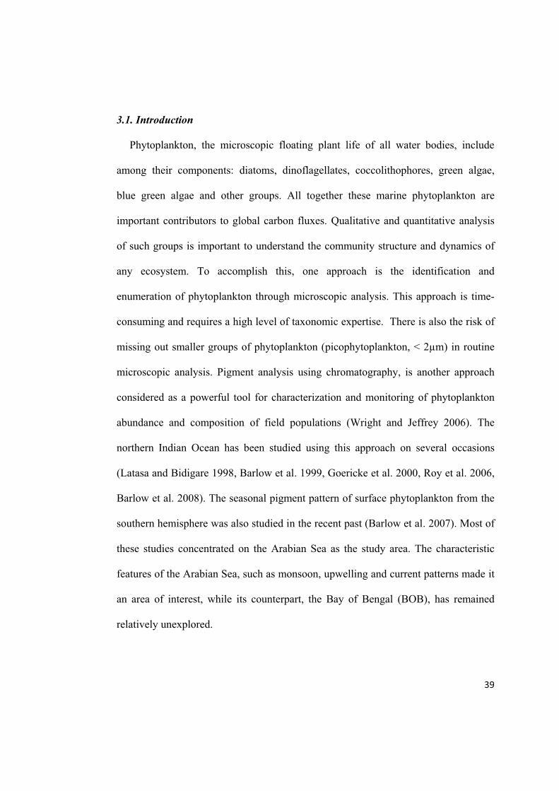
3.1. Introduction

Phytoplankton, the microscopic floating plant life of all water bodies, include

among their components: diatoms, dinoflagellates, coccolithophores, green algae,

blue green algae and other groups. All together these marine phytoplankton are

important contributors to global carbon fluxes. Qualitative and quantitative analysis

of such groups is important to understand the community structure and dynamics of

any ecosystem. To accomplish this, one approach is the identification and

enumeration of phytoplankton through microscopic analysis. This approach is time-

consuming and requires a high level of taxonomic expertise. There is also the risk of

missing out smaller groups of phytoplankton (picophytoplankton, < 2µm) in routine

microscopic analysis. Pigment analysis using chromatography, is another approach

considered as a powerful tool for characterization and monitoring of phytoplankton

abundance and composition of field populations (Wright and Jeffrey 2006). The

northern Indian Ocean has been studied using this approach on several occasions

(Latasa and Bidigare 1998, Barlow et al. 1999, Goericke et al. 2000, Roy et al. 2006,

Barlow et al. 2008). The seasonal pigment pattern of surface phytoplankton from the

southern hemisphere was also studied in the recent past (Barlow et al. 2007). Most of

these studies concentrated on the Arabian Sea as the study area. The characteristic

features of the Arabian Sea, such as monsoon, upwelling and current patterns made it

an area of interest, while its counterpart, the Bay of Bengal (BOB), has remained

relatively unexplored.

40

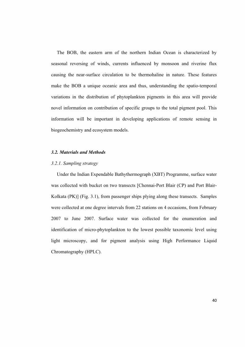
The BOB, the eastern arm of the northern Indian Ocean is characterized by

seasonal reversing of winds, currents influenced by monsoon and riverine flux

causing the near-surface circulation to be thermohaline in nature. These features

make the BOB a unique oceanic area and thus, understanding the spatio-temporal

variations in the distribution of phytoplankton pigments in this area will provide

novel information on contribution of specific groups to the total pigment pool. This

information will be important in developing applications of remote sensing in

biogeochemistry and ecosystem models.

3.2. Materials and Methods

3.2.1. Sampling strategy

Under the Indian Expendable Bathythermograph (XBT) Programme, surface water

was collected with bucket on two transects [Chennai-Port Blair (CP) and Port Blair-

Kolkata (PK)] (Fig. 3.1), from passenger ships plying along these transects. Samples

were collected at one degree intervals from 22 stations on 4 occasions, from February

2007 to June 2007. Surface water was collected for the enumeration and

identification of micro-phytoplankton to the lowest possible taxonomic level using

light microscopy, and for pigment analysis using High Performance Liquid

Chromatography (HPLC).

41

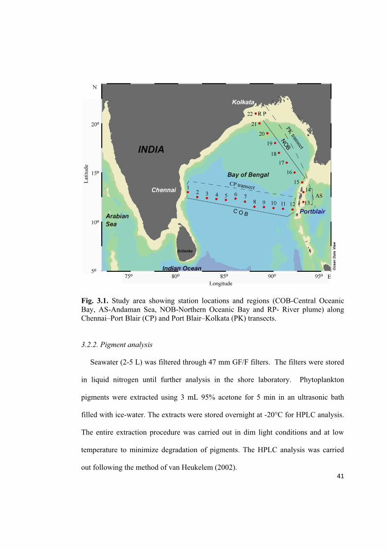
Fig. 3.1. Study area showing station locations and regions (COB-Central Oceanic

Bay, AS-Andaman Sea, NOB-Northern Oceanic Bay and RP- River plume) along

Chennai Port Blair (CP) and Port Blair Kolkata (PK) transects.

3.2.2. Pigment analysis

Seawater (2-5 L) was filtered through 47 mm GF/F filters. The filters were stored

in liquid nitrogen until further analysis in the shore laboratory. Phytoplankton

pigments were extracted using 3 mL 95% acetone for 5 min in an ultrasonic bath

filled with ice-water. The extracts were stored overnight at -20°C for HPLC analysis.

The entire extraction procedure was carried out in dim light conditions and at low

temperature to minimize degradation of pigments. The HPLC analysis was carried

out following the method of van Heukelem (2002).

42

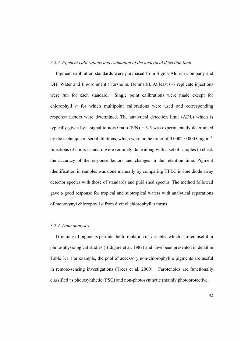
3.2.3. Pigment calibrations and estimation of the analytical detection limit

Pigment calibration standards were purchased from Sigma-Aldrich Company and

DHI Water and Environment (Hørsholm, Denmark). At least 6-7 replicate injections

were run for each standard. Single point calibrations were made except for

chlorophyll a for which multipoint calibrations were used and corresponding

response factors were determined. The analytical detection limit (ADL) which is

typically given by a signal to noise ratio (S/N) = 3-5 was experimentally determined

by the technique of serial dilutions, which were in the order of 0.0002-0.0005 mg m-3

.

Injections of a mix standard were routinely done along with a set of samples to check

the accuracy of the response factors and changes in the retention time. Pigment

identification in samples was done manually by comparing HPLC in-line diode array

detector spectra with those of standards and published spectra. The method followed

gave a good response for tropical and subtropical waters with analytical separations

of monovynyl chlorophyll a from divinyl chlorophyll a forms.

3.2.4. Data analyses

Grouping of pigments permits the formulation of variables which is often useful in

photo-physiological studies (Bidigare et al. 1987) and have been presented in detail in

Table 3.1. For example, the pool of accessory non-chlorophyll a pigments are useful

in remote-sensing investigations (Trees et al. 2000). Carotenoids are functionally

classified as photosynthetic (PSC) and non-photosynthetic (mainly photoprotective,

43

PPC) (Bidigare et al. 1990, Babin et al. 1996). The PSC pigments include

-hexanoyloxyfucoxanthin pigments, and are prominent in

regions of high productivity (Barlow et al. 2002). The PPC group includes

zeaxanthin, diadinoxanthin and diatoxanthin. This group is dominant in surface

waters with low chlorophyll and can account for up to 70% of the total pigment pool

(Gibb et al. 2001).

The ratios that can be derived from these pooled variables, for e.g., PSC/TChla,

are dimensionless and have the advantage of automatically scaling the comparison of

results from different areas and pigment concentrations. The diagnostic pigment (DP)

criteria was introduced by Claustre (1994) to estimate a pigment derive analog to the

f- ratio (the ratio of new production to total production). The use of DP was extended

by Vidussi et al. (2001) and more recently by Barlow et al. (2007) to derive size-

equivalent pigment indices which roughly correspond to the biomass proportions of

pico, nano and microplankton. Thus, DP can be used to understand the biomass

structure of an area purely based on pigment sums and ratios.

44

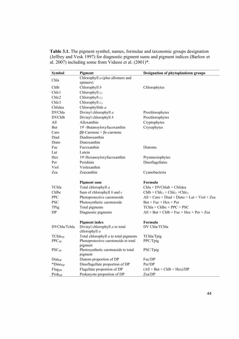
Table 3.1. The pigment symbol, names, formulae and taxonomic groups designation

(Jeffrey and Vesk 1997) for diagnostic pigment sums and pigment indices (Barlow et

al. 2007) including some from Vidussi et al. (2001)*.

Symbol Pigment Designation of phytoplankton groups

Chla Chlorophyll a (plus allomers and

epimers)

Chlb Chlorophyll b Chlorophytes

Chlc1 Chlorophyll c1



Chlidea Chlorophyllide a

DVChla Divinyl chlorophyll a Prochlorophytes

DVChlb Divinyl chlorophyll b Prochlorophytes

All Alloxanthin Cryptophytes

But 19' -Butanoyloxyfucoxanthin Crysophytes

Caro - -carotene

Diad Diadinoxanthin

Diato Diatoxanthin

Fuc Fucoxanthin Diatoms

Lut Lutein

Hex 19'-Hexanoyloxyfucoxanthin Prymnesiophytes

Per Peridinin Dinoflagellates

Viol Violaxanthin

Zea Zeaxanthin Cyanobacteria

Pigment sum Formula

TChla Total chlorophyll a Chla + DVChlab + Chlidea

Chlbc Sum of chlorophyll b and c Chlb + Chlc1 + Chlc2 +Chlc3

PPC Photoprotective carotenoids All + Caro + Diad + Diato + Lut + Viol + Zea

PSC Photosynthetic carotenoids But + Fuc + Hex + Per

TPig Total pigments TChla + Chlbc + PPC + PSC

DP Diagnostic pigments All + But + Chlb + Fuc + Hex + Per + Zea

Pigment index Formula

DVChla/Tchla Divinyl chlorophyll a to total

chlorophyll a

DV Chla/TChla

TChlaTP Total chlorophyll a to total pigments TChla/Tpig

PPCTP Photoprotective carotenoids to total

pigment

PPC/Tpig

PSCTP Photosynthetic carotenoids to total

pigment

PSC/Tpig

DiatDP Diatom proportion of DP Fuc/DP

*DinoDP Dinoflagellate proportion of DP Per/DP

FlagDP Flagellate proportion of DP (All + But + Chlb + Hex)/DP

ProkDP Prokaryote proportion of DP Zea/DP

45

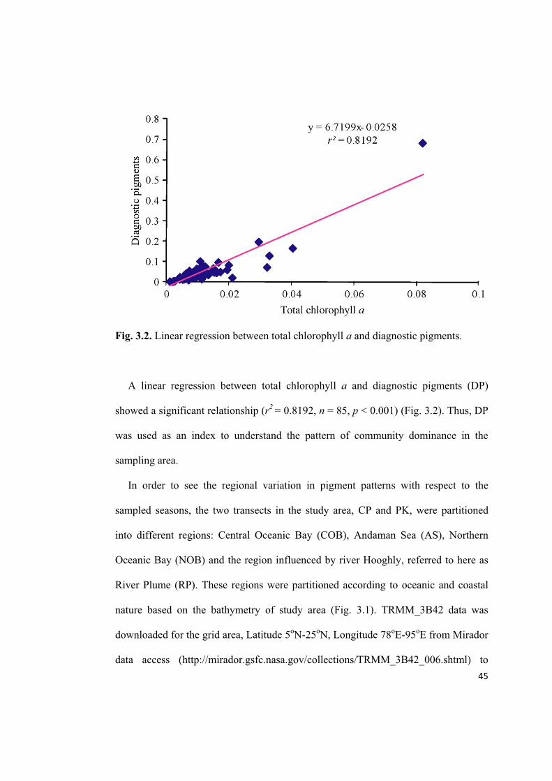
Fig. 3.2. Linear regression between total chlorophyll a and diagnostic pigments.

A linear regression between total chlorophyll a and diagnostic pigments (DP)

showed a significant relationship (r2

= 0.8192, n = 85, p < 0.001) (Fig. 3.2). Thus, DP

was used as an index to understand the pattern of community dominance in the

sampling area.

In order to see the regional variation in pigment patterns with respect to the

sampled seasons, the two transects in the study area, CP and PK, were partitioned

into different regions: Central Oceanic Bay (COB), Andaman Sea (AS), Northern

Oceanic Bay (NOB) and the region influenced by river Hooghly, referred to here as

River Plume (RP). These regions were partitioned according to oceanic and coastal

nature based on the bathymetry of study area (Fig. 3.1). TRMM_3B42 data was

downloaded for the grid area, Latitude 5oN-25

oN, Longitude 78

oE-95

oE from Mirador

data access (http://mirador.gsfc.nasa.gov/collections/TRMM_3B42_006.shtml) to

46

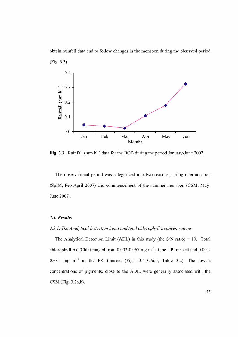
obtain rainfall data and to follow changes in the monsoon during the observed period

(Fig. 3.3).

Fig. 3.3. Rainfall (mm h-1

) data for the BOB during the period January-June 2007.

The observational period was categorized into two seasons, spring intermonsoon

(SpIM, Feb-April 2007) and commencement of the summer monsoon (CSM, May-

June 2007).

3.3. Results

3.3.1. The Analytical Detection Limit and total chlorophyll a concentrations

The Analytical Detection Limit (ADL) in this study (the S/N ratio) = 10. Total

chlorophyll a (TChla) ranged from 0.002-0.067 mg m-3

at the CP transect and 0.001-

0.681 mg m-3

at the PK transect (Figs. 3.4-3.7a,b, Table 3.2). The lowest

concentrations of pigments, close to the ADL, were generally associated with the

CSM (Fig. 3.7a,b).

47

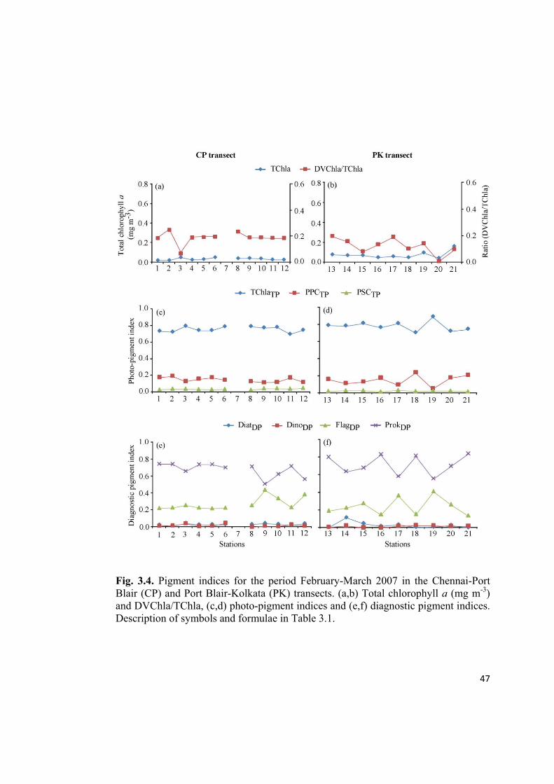
Fig. 3.4. Pigment indices for the period February-March 2007 in the Chennai-Port

Blair (CP) and Port Blair-Kolkata (PK) transects. (a,b) Total chlorophyll a (mg m-3

)

and DVChla/TChla, (c,d) photo-pigment indices and (e,f) diagnostic pigment indices.

Description of symbols and formulae in Table 3.1.

48

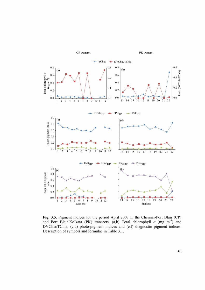
Fig. 3.5. Pigment indices for the period April 2007 in the Chennai-Port Blair (CP)

and Port Blair-Kolkata (PK) transects. (a,b) Total chlorophyll a (mg m-3

) and

DVChla/TChla, (c,d) photo-pigment indices and (e,f) diagnostic pigment indices.


49

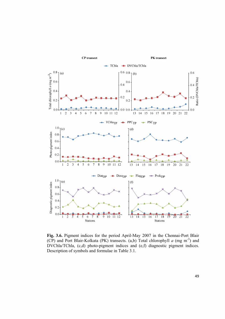
Fig. 3.6. Pigment indices for the period April-May 2007 in the Chennai-Port Blair

(CP) and Port Blair-Kolkata (PK) transects. (a,b) Total chlorophyll a (mg m-3

) and



50

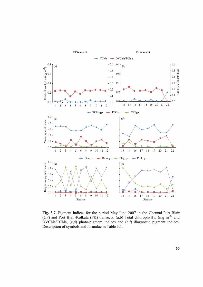
Fig. 3.7. Pigment indices for the period May-June 2007 in the Chennai-Port Blair

(CP) and Port Blair-Kolkata (PK) transects. (a,b) Total chlorophyll a (mg m-3

) and



51

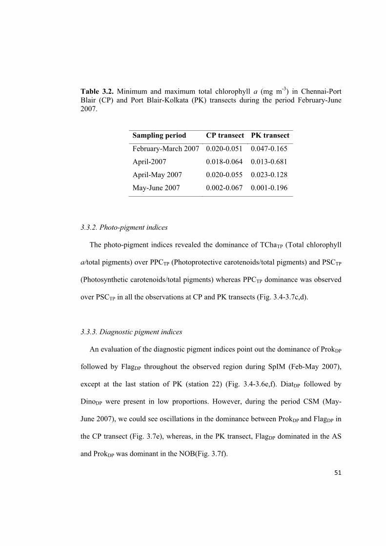
Table 3.2. Minimum and maximum total chlorophyll a (mg m-3

) in Chennai-Port

Blair (CP) and Port Blair-Kolkata (PK) transects during the period February-June

2007.

Sampling period CP transect PK transect

February-March 2007 0.020-0.051 0.047-0.165

April-2007 0.018-0.064 0.013-0.681

April-May 2007 0.020-0.055 0.023-0.128

May-June 2007 0.002-0.067 0.001-0.196

3.3.2. Photo-pigment indices

The photo-pigment indices revealed the dominance of TChaTP (Total chlorophyll

a/total pigments) over PPCTP (Photoprotective carotenoids/total pigments) and PSCTP

(Photosynthetic carotenoids/total pigments) whereas PPCTP dominance was observed

over PSCTP in all the observations at CP and PK transects (Fig. 3.4-3.7c,d).

3.3.3. Diagnostic pigment indices

An evaluation of the diagnostic pigment indices point out the dominance of ProkDP

followed by FlagDP throughout the observed region during SpIM (Feb-May 2007),

except at the last station of PK (station 22) (Fig. 3.4-3.6e,f). DiatDP followed by

DinoDP were present in low proportions. However, during the period CSM (May-

June 2007), we could see oscillations in the dominance between ProkDP and FlagDP in

the CP transect (Fig. 3.7e), whereas, in the PK transect, FlagDP dominated in the AS

and ProkDP was dominant in the NOB(Fig. 3.7f).

52

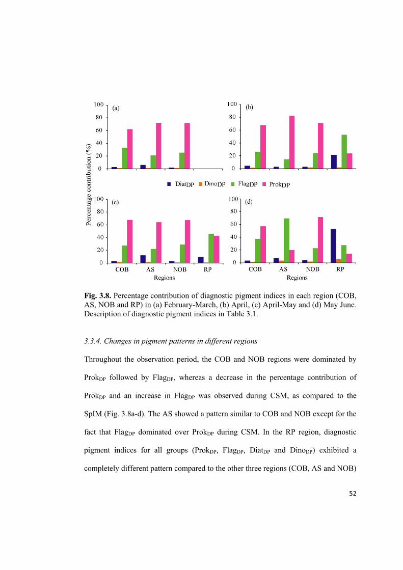
Fig. 3.8. Percentage contribution of diagnostic pigment indices in each region (COB,

AS, NOB and RP) in (a) February-March, (b) April, (c) April-May and (d) May June.

Description of diagnostic pigment indices in Table 3.1.

3.3.4. Changes in pigment patterns in different regions

Throughout the observation period, the COB and NOB regions were dominated by

ProkDP followed by FlagDP, whereas a decrease in the percentage contribution of

ProkDP and an increase in FlagDP was observed during CSM, as compared to the

SpIM (Fig. 3.8a-d). The AS showed a pattern similar to COB and NOB except for the

fact that FlagDP dominated over ProkDP during CSM. In the RP region, diagnostic

pigment indices for all groups (ProkDP, FlagDP, DiatDP and DinoDP) exhibited a

completely different pattern compared to the other three regions (COB, AS and NOB)

53

(Fig. 3.8a-d). The FlagDP diagnostic pigment index was dominant during the SpIM

observations (Fig. 3.8a-c), whereas the DiatDP index was dominant during the CSM

(Fig. 3.8d). A considerable increase in DinoDP was also observed during SpIM at the

RP region (Fig. 3.8d).

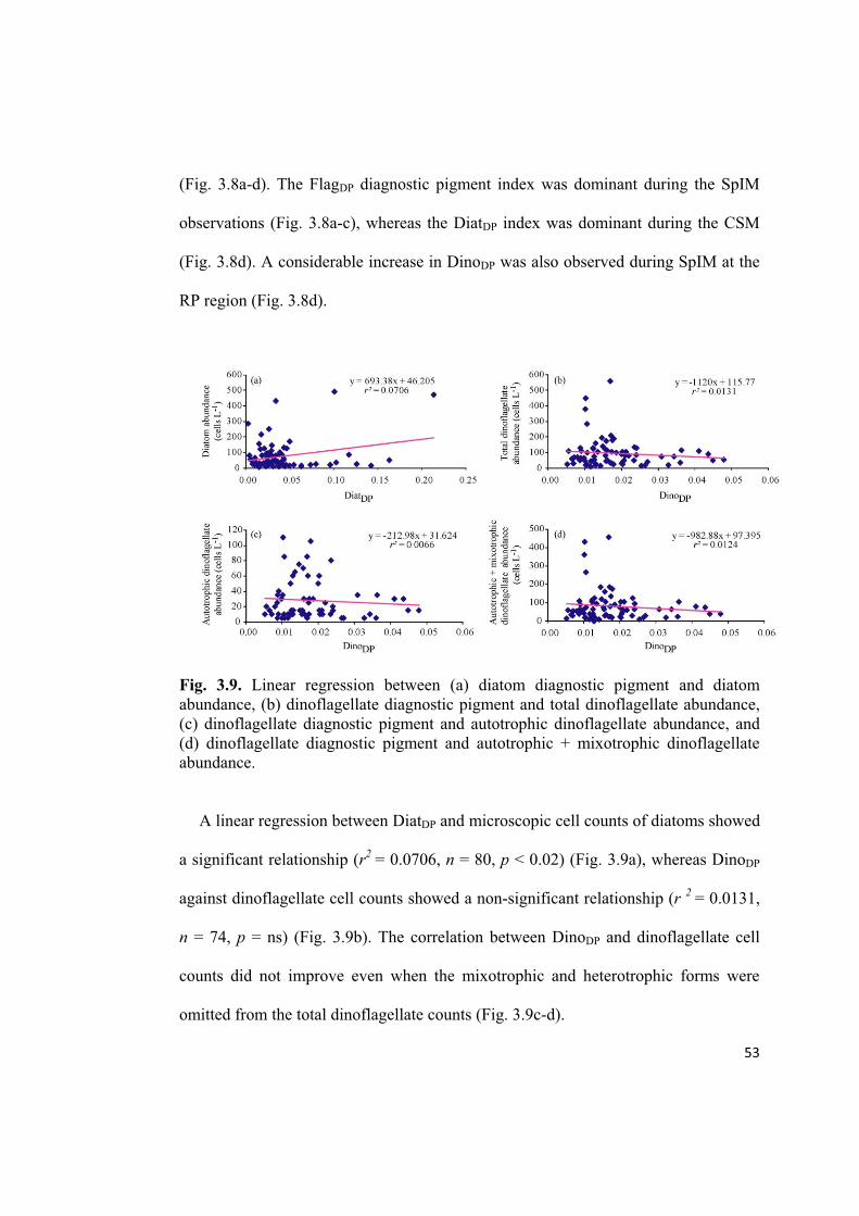
Fig. 3.9. Linear regression between (a) diatom diagnostic pigment and diatom

abundance, (b) dinoflagellate diagnostic pigment and total dinoflagellate abundance,

(c) dinoflagellate diagnostic pigment and autotrophic dinoflagellate abundance, and

(d) dinoflagellate diagnostic pigment and autotrophic + mixotrophic dinoflagellate

abundance.

A linear regression between DiatDP and microscopic cell counts of diatoms showed

a significant relationship (r2

= 0.0706, n = 80, p < 0.02) (Fig. 3.9a), whereas DinoDP

against dinoflagellate cell counts showed a non-significant relationship (r 2

= 0.0131,

n = 74, p = ns) (Fig. 3.9b). The correlation between DinoDP and dinoflagellate cell

counts did not improve even when the mixotrophic and heterotrophic forms were

omitted from the total dinoflagellate counts (Fig. 3.9c-d).

54

3.4. Discussion

The phytoplankton biomass evaluated so far in the region (Radhakrishna et al.

1978, Bhattathiri et al. 1980, Radhakrishna et al. 1982, Devassy et al. 1983, Sarma

and Aswanikumar 1991, Gomes et al. 2000, Prasanna Kumar et al. 2002,

Madhupratap et al. 2003) is based on fluorometer and spectrophotometer estimations

and remote-sensing values. The present study, based on HPLC pigment

characterization, is the first report from this area. In this study, the pigment

composition was characterized and evaluated in relation to the microscopic cell

counts of diatoms and dinoflagellates. The BOB is considered less productive as

compared to the Arabian Sea, due to strongly stratified surface waters (Prasanna

Kumar et al. 2002). It has been observed that such stratified conditions support the

dominance of prokaryotic groups (Chisholm 1992, Cullen et al. 2002). The

observations also indicated the dominance of ProkDP in the oceanic waters of the

BOB (Fig. 3.4-3.7e,f). In a recent study from the BOB, Hegde et al. (2008) observed

that stratified conditions support the prevalence of Trichodesmium, which is a

prokaryote with the ability to fix nitrogen. Thus, this prokaryote will have a

substantial input in new production in stratified waters. In the Baltic Sea, it has been

observed that nitrogen fixation by diazotrophs leads to the transfer of newly fixed

nitrogen to picoplanktonic organisms and supports the microbial foodweb

(Ohlendieck et al. 2000). In the present work, the DVChla/TChla ratio indicated the

dominance of Prochlorococcus sp. among the picoplankton group (Fig. 3.4-3.7a,b).

The metabolic properties of Prochlorococcus (Vaulot and Partensky 1992, Casey et

55

al. 2007, Martiny et al. 2009a) give them a flexible metabolism and the ability to

assimilate nitrate and nitrite (Martiny et al. 2009b). Hence, Prochlorococcus can

assimilate newly fixed nitrogen by micro-prokaryotes like Trichodesmium and

maintain its dominance in oceanic waters.

Earlier studies on accessory pigments from tropical latitudes demonstrated the

greater presence of PPCTP in surface, low chlorophyll waters (Stuart et al. 1998,

Gibb et al. 2000, Barlow et al. 2004). The observations from this study also indicate

that PPCTP tend to be high in surface waters during the SpIM period (Fig. 3.4-

3.7c,d). However, notable changes in the accessory pigments were observed with

increase of PSCs during CSM period at few stations of CP transect (Fig. 3.7c).

Similar changes were observed in the Atlantic, Pacific, Gulf of Oman and Arabian

Sea (Trees et al. 2000, Veldhuis and Kraay 2004). They observed that the change in

community structure is a physiological response to the changing environment

thereby resulting in changes in accessory pigments. In the present work, the change

in accessory pigments during CSM might be due to the responses of the community

to the changing environment influenced by rainfall. This indicates that

environmental and meteorological conditions may alter phytoplankton dynamics

through a chain of linked processes. These variations in accessory pigments in turn

are likely to affect the optical properties of phytoplankton which has implications for

ocean colour remote-sensing (Sathyendranath et al. 2005).

56

The second dominant group was the flagellates and their dominance in the AS

and RP near coastal regions (Fig. 3.7f) indicate their preference for nutrient-rich

coastal waters. Similarly, DiatDP also showed a preference for nutrient-rich turbulent

waters, being the dominant group at RP during the CSM (Fig. 3.7f). This change in

community structure could be linked to the increased rainfall during this season (Fig.

3.3). Thus a more significant change in community structure can be expected as

rainfall reaches its peak. Comparison of diagnostic pigments and microscopic cell

counts indicates that though a significant relationship between DiatDP and diatom

abundance was observed (Fig. 3.9a), it is pertinent to note that this significance was

arrived at even without considering the contribution of haptophytes, which also

contain fucoxanthin. In the case of DinoDP versus dinoflagellate abundance (Fig.

3.9b-d) the relationship was not significant. This suggests that peridinin as a marker

pigment did not work well for the dinoflagellate population in the region. In view of

this, further research comparing the HPLC pigment composition of dinoflagellates

with live cell abundances (to eliminate artifacts due to preservatives) should be

considered.

Summarizing the results, phytoplankton community structure in the BOB was

dominated by ProkDP followed by FlagDP with a low biomass of TChla, during the

study period. Changes in the pigment pattern were observed at the onset of the

monsoon, indicating the influence of rainfall especially in near coastal regions like

AS and RP. Comparative studies between microscopic counts and diagnostic pigment

57

indices suggest coupling pigment composition analysis with microscopic analysis of

natural assemblages to establish valid biogeochemical and ecosystem models.

Notably, the components of dinoflagellate communities could be missed by pigment

analysis alone.

Documents

Chap3.Primary description of surface water