Chapter 10 XV InformationLearning in Markets

Technical Appendix, Information and Learning in Markets by Xavier Vives December 2007

1

Technical Appendix This chapter reviews in a somewhat informal way some of the main tools used all along

the book. Accessible references to the material in this chapter can be found in Spanos

(1993, 2000) for probability and statistics, Laffont (1989) for information structures and

Fudenberg and Tirole (1991) for games. More advanced treatments can be found in De

Groot (1970), Ash (1972), Chung (1974), and Billingsley (1979) for probability and

statistics.

The workhorse model in the book is the linear-normal model and corresponding attention

is devoted to it. We start by having a look at information structures and the principles of

Bayesian inference in Section 1. We dedicate Section 2 to the study of the properties of

normal distributions and the affine information structure (to which the normal case

belongs and has the convenient property that conditional expectations are linear). Section

3 is devoted to convergence concepts of random variables and results, and properties of

Bayesian learning. Finally, Section 4 deals with Bayesian equilibrium.

1. Information structures and Bayesian inference

This section deals with some of the basics of probability (Section 1.1) and signals

(Section 1.2), the concept of sufficient statistic (Section 1.3), informativeness of

information structures (Section 1.4), and some useful concepts like properties of the

likelihood ratio and affiliation (Section 1.5). Section 1.6 presents some results with a

finite number of states.

1.1 Preliminaries

Given an arbitrary set Ω , we consider the space of states of nature ( Ω ,E ), where E is

the set of events: a collection of subsets of Ω ( i.e. 2Ω⊆E ). We put some restrictions on

the set of events: E is a σ -algebra or σ -field (a family of sets such that (i) the set Ω

belongs to it, (ii) if a set belongs to the family its complement also belongs to the family,

and (iii) the family is closed under countable unions of sets in the family). The space


2

( Ω ,E ) is then a measurable space and an event is a measurable set. A set in a given

class E is said to be E -measurable.

A probability measure on ( Ω ,E ) is a function [ ]P : 0,1→E such that P ( Ω ) =1 and for

every countable sequence of events, which are pairwise disjoint, the probability of the

union equals the (infinite) sum of the probabilities (this property is called countable

additivity). In the text the set of states will be a subset of Euclidean space. When ( Ω ,E )

is endowed with a probability measure P, the triple ( Ω ,E , P) is called a probability

space.

Given 1E and 2E two σ -fields of Ω , we will say that 1E is smaller than 2E if for any

1A ∈E , this implies 2A ∈E . The Borel σ -field is the one defined on the real line, and it is

the smallest containing all the closed intervals, for the Euclidean topology.

A random variable X on the probability space ( Ω ,E , P) is a real-valued function

X : Ω → such that for any ( )x ,∈ −∞ ∞ , the set ( ) : X xω∈Ω ω ≤ is an event (belongs

to E ). A real-valued function fulfilling this property is called measurable with respect to

E or E -measurable. A random variable induces a probability measure on the Borel

subsets of the reals: ( ) ( ) XP B P : X B= ω∈Ω ω ∈ where B is a Borel subset. A support

for the probability measure induced by the random variable X is a Borel set of full

measure. The distribution function of the random variable X is [ ]F : 0,1→ such that

( ) ( ) F x P : X x= ω∈Ω ω ≤ .

A random vector is a mapping kX : Ω → E -measurable. It is a k-tuple of random

variables ( )1 kX X ,..., X= . We have that ( ) ( ) ( )( )1 kX X ,..., Xω = ω ω for ω∈Ω and X is

E -measurable if and only if each iX is. The σ -field generated by the random vector X is

the smallest σ -field with respect to which it is measurable and is denoted by ( )Xσ (i.e.


3

the smallest -fieldσ generated by the events of the type ( )1iX B− with B a Borel set of the

real line and i 1,..., k= ). This is a sub- σ -field of ( Ω ,E ).

Let ΒΑ, be events in a probability space ( Ω ,E , P) with ( ) 0>ΒΡ . The conditional

probability of Α given Β is ( ) ( ) ( )P A | B P A B P B= ∩ . This is the probability that an

observer assigns to ω∈Ω to lie in A if he learns that ω lies in B. More in general we can

define the conditional probability of A given a sub- σ -field G of ( Ω ,E ) and denote it by

( )P A | G . The σ -field G may come, for example, from a partition of Ω or may be more

general, and it can be identified with an observation or experiment (an observer may know for each B∈G whether ω lies in B or not). ( )P A | G is a random variable which is

G -measurable, integrable, and satisfies the functional equation

( ) ( )B

P A | dP P A B= ∩∫ G for B∈G . Any random variable fulfilling those properties is

a version of the conditional probability and any two versions are equal with probability 1. The conditional probability of A given a random variable X is defined as ( )( )P A | Xσ

and denoted by ( )P A | X . In a similar way we can define the conditional expectation.

Suppose that X is an integrable random variable on ( Ω ,E , P) and G a sigma field in E .

The conditional expected value of X given G is the random variable [ ]E X | G which is

G -measurable, integrable and which satisfies the functional equation

[ ]B B

E X | dP XdP=∫ ∫G for B∈G . Any random variable fulfilling those properties is a

version of the conditional expected value and any two versions are equal with probability

1. The conditional expected value of X given the sigma field generated by the random variable Y , ( )Yσ , is ( )E X | Yσ⎡ ⎤⎣ ⎦ and denoted by [ ]E X | Y .

The following rule is the basis to update probabilities.


4

The rule of Bayes: Let ,..., 21 ΑΑ be an infinite sequence of disjoint events with

( )iP A 0> for any i and such that their union is Ω . Let Β be another event such that

( )P B 0> . Then

( ) ( ) ( )( ) ( )

i ii

j jj 1

P B | A P AP A | B i 1, 2,...

P B | A P A∞

=

= =∑

A similar result applies to a finite sequence of disjoint events n1 A,...,A (see De Groot

(1970, p.11-12)).

Remark on notation: To simplify notation in general we will not distinguish between a

random variable X and its realization x, and we use the lower case notation.

1.2 Information structures

Consider the space of states of nature (Θ, E ) and a probability space (Θ,E , P). We may

assume, as is typically done in the text, that the agent knows the probability distribution

P. This is called the prior distribution. However, the agent may also have a subjective

prior probability assessment that need not coincide with the objective prior.

The information available to an agent can be described by a partition of the state space

Θ. Equivalently, by a (measurable) function : Sφ Θ → where S is a space of signals. In

this case the corresponding partition of Θ is given by the elements ( )1 s−φ , s S∈ . When

the agent receives a signal he learns in which element of the partition lies the state of

nature. This formulation corresponds to an information structure without noise.

The signals received by the agent are typically noisy. Then for every state of the world in

Θ, a nondegenerate distribution is induced on the (measurable) signal space S. A usual

case is to have for each θ a conditional density ( )h s θ defining the likelihood function of

the signals received by the agent. The information structure is given then by a space of

signals and a likelihood function (S, ( )h ⋅ θ ), which defines a random variable,

“experiment”, or signal s with values in S (recall that we do not distinguish notationally


5

between a random variable and its realization). This implies, obviously, that the random

variable s has a probability distribution which depends on θ .

Once the agent receives the signal s he updates his distribution on θ according to the rule

of Bayes and forms a posterior distribution of θ given s. Suppose that the prior distribution is given by the density ( )f θ and the likelihood by the conditional density

( )h s θ . Denote the posterior density or conditional density of θ given the observation of

s by ( )f sθ . According to (the continuous distribution version of ) the rule of Bayes we

have that

( ) ( ) ( )( ) ( )h s f

f sh s f d

θ θθ =

θ θ θ∫.

With discrete distributions we have an analogous result. 1.3 Sufficient statistics

Any function Ψ of the observation of the random variable or vector s is called statistic.

A statistic Ψ is called a sufficient statistic if for any prior distribution of θ , its posterior

distribution depends on the observed value of s only through ( )sΨ . In this case to obtain

the posterior distribution of θ from any prior, the agent only needs the value of ( )sΨ .

More formally, a statistic Ψ is a sufficient statistic for a family of distributions

( ) h ,⋅ θ θ∈Θ if ( ) ( )f s f s′ ′′⋅ = ⋅ for any prior ( )f ⋅ and any two points s S′∈ and s S′′∈

such that ( ) ( )s s′ ′′Ψ = Ψ .

A useful characterization of sufficiency is the factorization criterion (De Groot (p.155-156, 1970): A statistic Ψ is sufficient for a family of distributions ( ) h ,⋅ θ θ∈Θ if, and

only if, for any s in S and θ∈Θ ; ( )h s θ can be factored as follows:

( ) ( ) ( )( )h s u s v s ,θ = Ψ θ


6

where the function u is positive and does not depend on θ , and the function v is

nonnegative and depends on s only through ( )sΨ .

For example, suppose an agent observes signals 1 ns ,...,s which are a random sample

from a Gaussian normal distribution with unknown value of the mean θ and known

variance 2 0σ > . That is, the likelihood ( )h ⋅ θ is normal with mean θ and

variance 2 0σ > . Then the conditional joint probability density function is

( ) ( ) ( )

( )

( )

nn 22 2

n 1 n i2 i 1

n 2n n2 22

i i2 2 2i 1 i 1

n 2n n2 22

i i2 2 2i 1 i 1

1h s ,...,s 2 exp s2

1 n2 exp s s2 2

1 n2 exp s exp s2 2

−

=

−

= =

−

= =

⎧ ⎫θ = πσ − − θ⎨ ⎬σ⎩ ⎭⎧ ⎫θ θ

= πσ − − −⎨ ⎬σ σ σ⎩ ⎭⎧ ⎫θ θ⎧ ⎫= πσ − − −⎨ ⎬ ⎨ ⎬σ σ σ⎩ ⎭ ⎩ ⎭

∑

∑ ∑

∑ ∑

Letting ( ) ( )n

n2 22i2 i 1

1u s 2 exp s2

−

=

⎧ ⎫= πσ −⎨ ⎬σ⎩ ⎭∑ , ( ) n

ii 1s s

=Ψ = ∑ , and

( )( ) ( )2

2 2

nv s , exp s2

⎧ ⎫θ θΨ θ = − Ψ −⎨ ⎬σ σ⎩ ⎭

, we have that ( )n 1 nh s ,...,s θ can be factored

according to the criterion and ( ) nii 1

s s=

Ψ = ∑ is a sufficient statistic. Note that sufficient

statistics are not unique. Indeed, for example, the average signal ( )nii 1

s s n=

= ∑% is also a

sufficient statistic (use the decomposition ( ) ( ) ( )n n2 2 2i ii 1 i 1

s s s n s= =

− θ = − + − θ∑ ∑ % % ).

1.4 Informativeness of signals

If the information structure is given in partition form of the state space then one partition

is more informative than another if it is finer (i.e. if each element of the latter can be

obtained as the union of elements of the former). It should be clear that with a finer

partition a decision maker can not do worse because with the finer one he can always


7

make decisions based only on the coarser one. Any decision maker, for any utility

function and prior distribution on Θ, will prefer one information structure to another if

and only if the former is finer than the latter. More information can not hurt. This may

not be true when there is interaction among different players. In fact, then an

improvement in information can make everyone worse off.

Blackwell (1951) developed the concept of an information structure or experiment ( )S, h

being sufficient for information structure or experiment ( )S , h′ ′ when, intuitively,

independent of the value of θ, s′ can be obtained from s by adding noise. If this is the

case then an agent should never perform the experiment s′ when s is available. We say

that signal s is more informative than signal s′ if s is sufficient (in the Blackwell sense)

for signal s′ .

For continuously distributed signals, we say that signal s is sufficient for signal s′ if there

exists a stochastic transformation from s to s′ -i.e. a function g :S xS +′ → where

S'g(s ,s) ds 1′ ′ =∫ for any s in S (and assume also for convenience that g is integrable, with

positive value, with respect to s for any s′ )- such that ( ) ( ) ( )S

h s g s ,s h s ds′ ′ ′θ = θ∫ for

any θ in Θ and s′ in S′ . Note that ( )g ,s⋅ is a probability density function for any s in S

since a realization s′ can be generated by a randomization using ( )g ,s⋅ given that

S'g(s ,s) ds 1′ ′ =∫ for any s in S (see De Groot (1970, p.434)).

For example, consider the case where both the prior distribution and likelihood are given

by the Gaussian normal distribution function: θ with mean θ and finite variance 2θσ

(and we write ( )2~ N , θθ θ σ ) and s conditional on θ with mean θ and finite variance 2εσ

(and we write ( )2s | ~ N , εθ θ σ ). That is, s = θ + ε , where ( )2~ N 0, εε σ and [ ]cov , 0θ ε = .

The precision of the signal (likelihood) is defined to be the inverse of the


8

variance: ( ) 12 −

ε ετ = σ . Then it is immediate that s is more informative than s′ if and only

if ′ε ετ > τ since s′ can be obtained from s by adding noise.

A similar definition can be given for the case of discrete signals. If the number of

possible states and signals is finite, then an information structure is characterized by the pair ( )S,L , where S has a finite number of elements and L is the likelihood matrix with

entries of the type ( )k jP s θ . Then information structure ( )S,L is sufficient or more

informative than ( )S ,L′ ′ if and only if there is a conformable Markov matrix M (i.e. a

matrix with nonnegative elements with columns adding up to 1) such that L ML′ = .

Blackwell’s theorem states that any decision maker, for any utility function and prior distribution on Θ, should prefer information structure ( )S, h to ( )S , h′ ′ if and only if s is

sufficient for signal s′ (Blackwell (1951); see also Cremer (1982) and Kihlstrom (1984)).

A more informative signal corresponds to a finer information partition.

1.5 Some useful concepts Suppose that the agent has a prior density ( )f θ on Θ ⊂ and the likelihood is given by

the conditional density ( )h s θ and, as before, denote the posterior density by ( )f | sθ .

According to the rule of Bayes we have that

( ) ( )( )

h(s | )f f | s

h(s | )f dθ θ

θ =θ θ θ∫

.

From the rule of Bayes we obtain the likelihood ratio for any two states ′θ and θ :

( )( )

( )( )

( )( )

f | s h s | ff | s h s | f

′ ′ ′θ θ θ=

θ θ θ.


9

The family of likelihoods ( ) h |⋅ θ has the monotone likelihood ratio property (MLRP)

if for every ′θ > θ and ˆs s> we have that ( ) ( ) ( ) ( )ˆ ˆh s | h s | h s | h s | 0′ ′θ θ − θ θ ≥ . This

means that the likelihood ratio ( ) ( )h s | / h s |′θ θ is increasing in s for 'θ > θ . A larger

realization of s is to be interpreted as news that the likelihood is more likely to be

( )h s | 'θ than ( )h s | θ . Many of the commonly used densities satisfy the MLRP.

Examples are the normal distribution, the exponential distribution, or the Poisson

distribution, all three with mean θ ; the uniform distribution on [ ]θ,0 , or the chi-squared

distribution (with noncentrality parameter θ ) (see Milgrom (1981)).

Affiliation. If the real valued function kf : → is twice-continuously differentiable we

say it is log-supermodular if and only if 2i jlog f / x x 0∂ ∂ ∂ ≥ for all i j≠ .1 Suppose that

the (real valued) random variables 1 kx ,..., x have a joint density ( )f ⋅ . The random

variables are affiliated if their joint density is log-supermodular (almost everywhere).

Milgrom and Webber (1982) provide a general definition of affiliation.

For convenience suppose that the support of the family of densities ( ) h |⋅ θ is

independent of θ . An equivalent way to express the MLRP is to say that

( )log h s | /∂ θ ∂θ is increasing in s (or ( )2 log h s | / s 0∂ θ ∂θ∂ ≥ if ( )h |⋅ ⋅ is twice-

continuously differentiable). (We can think of ( )ln h s | θ as the likelihood function of the

model where s is the estimator for the parameter θ .) The condition is the equivalent to

log-supermodularity of ( )h s | θ . In turn, this would be equivalent to log-supermodularity

of

the joint density ( ) ( ) ( )f s, h s | fθ = θ θ . We say then that the random variables s and θ

are affiliated.

1 In Section 4.1 we provide a more general definition of supermodularity and log-supermodularity.


10

The MLRP property implies first order stochastic dominance (FOSD). If the family of likelihoods ( ) h |⋅ θ has the MLRP then for any nondegenerate prior distribution F for θ

the posterior distribution ( )F | s⋅ first order stochastically dominates ( )F | s′⋅ for s s′>

(see Milgrom (1981)). We say that the distribution ( )F ; yθ is ordered by the parameter y

according to first-order stochastic dominance if ( )F ; yθ is decreasing in y.

1.6 Finite number of states

Two-point support information structure. A simple example of a discrete information structure is the two–state space L H,Θ = θ θ , with respective prior probabilities ( )LP θ

and ( )HP θ , and two–point support signals L HS s ,s= model. The agent may receive a

low ( )Ls or a high ( )Hs signal about θ with likelihood ( ) ( )H H L LP s P s qθ = θ = ,

where 1 q 12

≤ ≤ . With this setup we have a symmetric binary model. If 1q2

= the signal

is uninformative; if 1q = , it is perfectly informative. It is easily checked that s is more

informative than s′ if and only if qq ′> . Indeed, the likelihood matrix associated to s′ , q ' 1 q '

L1 q ' q '

−⎡ ⎤′ = ⎢ ⎥−⎣ ⎦, can be obtained with a stochastic transformation of the likelihood

matrix associated to s , q 1 q

L1 q q

−⎡ ⎤= ⎢ ⎥−⎣ ⎦

since L ML′ = , where

( )( )

( )q ' 1 q q q '1M

q q ' q ' 1 qq 1 q− − −⎡ ⎤

= ⎢ ⎥− − −− − ⎣ ⎦ is a Markov matrix.

The logarithm of the likelihood ratio (LLR) of the two states

( ) ( )( )H Llog P / Pλ = θ θ updates in an additive way with new information. (This

generalizes to any two states out of a finite number). After observing signal s (be it from

a discrete or a continuous likelihood) it is immediate from the rule of Bayes that the

updated LLR is

( ) ( )( )H Llog P s / P sθ θ = ( )sλ + λ where ( ) ( ) ( )( )H Ls log P s / P sλ = θ θ .


11

One possible way to define signals of bounded strength is to look at the LLR. A signal

will be of bounded strength if the support of the distribution of the LLR is bounded. This

is clearly the case with the two point support information structure. It would not be the case if the likelihood is normally distributed ( )1s | ~ N , −

εθ θ τ . That is, ε+θ=s where

( )1~ N 0, −εε τ with [ ]cov , 0θ ε = . Letting ( ) ( )H LP P 1/ 2θ = θ = we have, since

( ) ( ) 2P s exp s / 2εθ = −τ − θ , that ( ) ( ) ( )( )H L H Ls s / 2ελ = τ θ − θ − θ + θ . Then the

support of ( )sλ is unbounded since s is normally distributed (see Chamley (2003) and

Smith and Sorensen (2000) for applications).

2. Normal distributions and affine information structure

Gaussian distributions have the convenient property, among others as we shall see, that

conditional expectations are linear (affine to be precise but we will use often the term

“linear” instead of “affine”). This proves crucial in obtaining linear equilibria in games

with quadratic payoffs or negative exponential utility. However there are other pairs of

prior and likelihood that yield also conditional linear expectations.

2.1 The Gaussian distribution A random variable x has a normal distribution with mean [ ]E xµ = and variance

[ ]2 var xσ = > 0 if it is continuously distributed with density at any point x−∞ < < ∞ given by

( )21 1 xf x exp

22

⎧ ⎫− µ⎪ ⎪⎛ ⎞= −⎨ ⎬⎜ ⎟σπσ ⎝ ⎠⎪ ⎪⎩ ⎭.

We write ( )2x ~ N ,µ σ . The normal density is completely characterized by two parameters: mean and variance. An immediate implication is the following: if

( )2x ~ N ,µ σ and y x= α + β , where α and β are constants, then we have

( )2 2y ~ N ,α + βµ β σ . It follows that if ( )2x ~ N ,µ σ , then xz − µ≡

σ is ( )N 0,1 , which is

the standard normal random variable. The following facts will prove useful:


12

• If ( )2x ~ N ,µ σ and β is a constant then 2 2E exp x exp / 2β = βµ + β σ⎡ ⎤⎣ ⎦ .

• If ( )2x ~ N 0,σ then E[| x |] 2= σ π .

We can define similarly a multivariate normal distribution. Consider an n -dimensional normal random variable ( ) ( ),s ~ N ,θ µ Σ , with nµ ∈ and variance-covariance matrix

n n×Σ ∈ . The mean vector and variance-covariance matrix can be partitioned as , ,s

s, s,ss

; θ θ θθ

θ

Σ Σµ ⎡ ⎤⎡ ⎤µ = Σ = ⎢ ⎥⎢ ⎥ Σ Σµ⎣ ⎦ ⎣ ⎦

.

Then marginal distributions for ( ),~ N ,θ θ θθ µ Σ and ( )s s,ss ~ N ,µ Σ are normal. The conditional expectation is characterized uniquely by the projection theorem for normal random variables: E s⎡θ ⎤⎣ ⎦ is the unique linear function of ( ),sθ such that

[ ]E E s E⎡ ⎤⎡θ ⎤ = θ⎣ ⎦⎣ ⎦ and

cov E s ,s 0⎡ ⎤θ − ⎡θ ⎤ =⎣ ⎦⎣ ⎦ .

The first property is just the law of iterated expectations. The second has a geometric interpretation. Say that θµ = sµ = 0, then E s⎡θ ⎤⎣ ⎦ is the projection of θ onto the subspace

generated by the components of s (where random variables are seen as elements of a

functional space: the Hilbert space of square integrable functions (see Loeve (1955)).

It follows then (see Anderson (1958) and De Groot (1970, Ch. 5, section 4)) that the conditional density of θ given s is normal with conditional mean ( )1

,s s,s ss−θ θµ + Σ Σ − µ

and variance-covariance matrix 1, ,s s,s s,

−θ θ θ θΣ − Σ Σ Σ , provided s,sΣ is non-singular, (i.e.

( ) ( )( )1 1,s s,s s , ,s s,s s,| s ~ N s ,− −

θ θ θ θ θ θθ µ + Σ Σ − µ Σ − Σ Σ Σ ).

It is worth noting that the conditional variance-covariance matrix does not depend on the

signal realization s. This is a special feature of the normal distribution which simplifies

computations. Linear combinations of normal random variables are also normal and, if x and y are bivariate normal and [ ]cov x, y 0= , then x and y are independent.


13

The projection characterization has a very important consequence: the conditional expectation E s⎡θ ⎤⎣ ⎦ is a sufficient statistic for the information s. In order to update

beliefs about θ knowing E s⎡θ ⎤⎣ ⎦ provides the same information as knowing s. The

following claim illustrates the result.

Claim: Suppose ( ),sθ are jointly normally distributed and let

[ ]E | sη = θ − θ

then η and E s⎡θ ⎤⎣ ⎦ are independent random variables. The conditional distribution of θ

given s is the same as the conditional distribution of θ given ( )s E sϕ ≡ ⎡θ ⎤⎣ ⎦ : both

distributions are normal, with mean

[ ] ( )E | s E | sθ = θ ϕ⎡ ⎤⎣ ⎦

and variance

[ ] ( ) [ ]var | s var | s varθ = θ ϕ = η⎡ ⎤⎣ ⎦ .

Proof: We know that E s⎡θ ⎤⎣ ⎦ is a linear function of s and therefore (since linear functions

of normal random variables are normal) both E s⎡θ ⎤⎣ ⎦ and [ ]E | sη = θ − θ are normal. We

have that [ ] [ ] [ ]E E E E | s 0⎡ ⎤η = θ − θ =⎣ ⎦ . From the projection characterization

[ ]cov ,s cov E s ,s 0⎡ ⎤η = θ − ⎡θ ⎤ =⎣ ⎦⎣ ⎦ and therefore

[ ] [ ] [ ] [ ]var var E | s var E | s var⎡ ⎤ ⎡ ⎤θ = θ + η = θ + η⎣ ⎦ ⎣ ⎦ .

We have that the conditional distribution of [ ]E | sθ = θ + η given s is normal (since both

( )s E sϕ ≡ ⎡θ ⎤⎣ ⎦ and η are normal) with mean ( )E s E s⎡ ⎤⎡θ ⎤ = θ ϕ⎣ ⎦ ⎣ ⎦ and

[ ] [ ] [ ] ( )var | s var | s var var | sθ = η = η = θ ϕ⎡ ⎤⎣ ⎦ , and normal random variables are fully characterized by mean and variance. ◊

Example: If both θ and s are one-dimensional then we have that

( ) ( ) ( )2 2s

s

| s ~ N s , 1θθ θ

⎛ ⎞σθ µ + ς − µ σ − ς⎜ ⎟σ⎝ ⎠

,


14

where letting sθσ = [ ]cov ,sθ , s

s

θ

θ

σς =

σ σ is the correlation coefficient between θ and s

and [ ][ ]s

cov ,svar s

θ θσς =

σ. Provided that the signal is unbiased (i.e. E s⎡ θ⎤ = θ⎣ ⎦ ), the signal

can be interpreted as being the sum of the true θ plus (orthogonal) noise: s = θ + ε , with

( )2N 0, εε σ and [ ]cov , 0θ ε = . (According to the projection characterization,

cov s E s , 0⎡ ⎤− ⎡ θ⎤ θ =⎣ ⎦⎣ ⎦ , and therefore for an unbiased signal, [ ]cov s , 0− θ θ = ). Denote

by 2x x1/τ ≡ σ the precision of the random variable x. In terms of the posterior

distribution, we have that the precision of the signal is given by θ ετ + τ (i.e.

( ) 1var s −θ ε⎡θ ⎤ = τ + τ⎣ ⎦ ). The (posterior) precision of the signal is given by the sum of the

precision of the prior θτ and the precision of the signal ετ . The signal can be thought of

coming from a sample of (conditionally) independent observations from ( )2N ,θ σ . A

sufficient statistic for θ is the sample mean. Therefore for a k-sample we have that 2 2 / kεσ = σ . The precision of the signal s (the sample mean) is therefore proportional to

the size of the sample.

The posterior mean can be written also as

( )E s s 1 θ⎡θ ⎤ = ξ + − ξ µ⎣ ⎦ where [ ][ ]

2

s

cov ,svar s

θ ε

θ ε

θ σ τξ = = ς = ς =

σ τ + τ.

The coefficient ξ is the typical regression coefficient of θ on s ( [ ][ ]

cov ,svar s

θ) and the

square of the correlation coefficient between θ and s. We have thus that [ ]E | sθ is a

weighted average of the signal and the prior mean with weights according to the relative

precisions. When the signal is perfect ( 2 0εσ = ) and 1ξ = , when the signal is useless

( 2εσ = ∞ ) 0ξ = . Another useful property is that the precision of conditionally

independent signals is additive. This is illustrated in the next example.


15

Example: Suppose we have n signals i is = θ + ε , i 1,..., n= , where the noise terms iε have

mean zero and are independent of θ and of each other. Then the conditional mean and

variance of θ are given by

[ ] ( )i

i

n1 n in i 1

i 1

1E | s , ..., s sθ ε θ=θ ε=

θ = µ + τ − µτ + τ

∑∑

[ ]i

1 n n

i 1

1var | s , ..., sθ ε=

θ =τ + τ∑

.

The conditional precision is

1 n i

n|s , ..., s i 1θ θ ε=

τ = τ + τ∑ .

It follows that the precision-weighted signal average

( )i i

1n nn ii 1 i 1

s s−

θ ε ε= == τ + τ τ∑ ∑%

is a sufficient statistic for the signals 1 ns , ..., s . If all iε are identically distributed with

common precision ετ , then

[ ] n1 n ii 1

1 1E | s , ..., s n sn nθ ε θ=

θ ε

⎛ ⎞θ = µ + τ − µ⎜ ⎟τ + τ ⎝ ⎠∑ .

Normal distributions have very convenient and intuitive properties. Linear combinations

of normal random variables are normal, and conditional expectations are also linear in

signals. A Bayesian agent in a normal world will put more weight to a signal which is

more precise. The rules to update the precision of information are additive for

conditionally independent signals and do not depend on the realization of information. A

new signal increases total precision according to its precision. This has the consequence

that new information adds precision independently of the realization of the new signal.

Finally, as we will see, normal distributions fit very nicely with models where agents end

up optimizing a quadratic function.


16

Some of the convenient properties of normal distributions are robust in other scenarios.

Suppose that an unknown parameter θ with finite variance is to be estimated from the observations n

1 nz z ,..., z= where t t tz a u= θ + , where ta are known constants, t = 1,..,

n, and tu are i.i.d. random variables with zero mean and finite variance 2uσ . We know

that, under general distributions, nE z⎡ ⎤θ⎣ ⎦ is the unique best predictor of θ in the sense of

minimizing the mean squared error (under normality nE z⎡ ⎤θ⎣ ⎦ is linear and depends only

on first and second moments). With finite second moments ( )2 2u,θσ σ the unique best

(mean squared error) linear predictor of θ based on nz (that is, the linear function

( ) nn0 k kk 1

z z=

δ = α + α∑ which minimizes ( )( )2nE z⎡ ⎤θ − δ⎢ ⎥⎣ ⎦ over the α coefficients) is

given by the same expression as under normality:

( )nnu k k nk 1

E z a z /θ =⎡ ⎤θ = τ θ + τ τ⎣ ⎦ ∑

where n 2n u kk 1

aθ =τ = τ + τ ∑ .

This implies that if agents have limited forecasting ability and use linear prediction to

estimate θ the same result as under normality will be obtained (since the best linear predictor of θ based on nz is precisely nE z⎡ ⎤θ⎣ ⎦ ). We will see in the next section other

information structures which preserve the linearity of conditional expectations.

2.2 Affine information structure

Some of the convenient properties of normal distributions are also enjoyed for other pairs

of prior and likelihood functions. Indeed, the pair normal – normal is only one example

of the class for which conditional expectations are linear (affine). For example, the pairs

of prior and likelihood beta-binomial and gamma-Poisson have the affine conditional

expectation property. In this case, as in the normal-normal case the sample mean is a


17

sufficient statistic for θ . Other cases are when the observations are conditionally

independent negative binomial, gamma, or exponential when assigned natural conjugate

priors.( See DeGroot (1970), Ericson (1969), and Li et al (1987).)

When the precision of a signal s about θ ( ) 1

var s−

⎡ θ⎤⎣ ⎦ is not independent of the state we

consider the inverse of the expected conditional variance r = [ ]( ) 1E var s |

−⎡ ⎤θ⎣ ⎦ . In terms

of the posterior distribution the precision of the signal s about θ is then [ ]( ) 1E var | s

−⎡ ⎤θ⎣ ⎦ .

If the signal is unbiased ( [ ]E s | θ = θ ), letting sε = − θ we have also that [ ]cov , 0ε θ =

and [ ] [ ]var E var s |⎡ ⎤ε = θ⎣ ⎦ . Indeed, [ ] [ ] 2cov s , E s E ⎡ ⎤− θ θ = θ − θ⎣ ⎦ , and by the law of

iterated expectations [ ] ( ) [ ] 2E s E E s | E E s | E ⎡ ⎤⎡ ⎤θ = θ θ = θ θ = θ⎡ ⎤⎣ ⎦ ⎣ ⎦ ⎣ ⎦ if [ ]E s | θ = θ . We

have then [ ] [ ] [ ] [ ] [ ]var s var var var E s | E var s |⎡ ⎤ ⎡ ⎤= θ + ε = θ + θ⎣ ⎦ ⎣ ⎦ since [ ]E s | θ = θ and

therefore [ ] [ ]var E var s |⎡ ⎤ε = θ⎣ ⎦ . The precision of the signal is denoted as usual by ετ . A

more precise signal implies a smaller mean squared prediction error [ ]( )2E E | s⎡ ⎤θ − θ

⎣ ⎦.

If the prior distribution is beta with parameters ( ),α β on the interval ( )0,1 (where

0α > and 0β > ) and the signal is the average of n independent Bernoulli trials with

parameter θ , then the likelihood of the signal is n1 binomial ( )θ,n with ( )r nθ= τ α + β

and the posterior distribution is ( )( )s1n,nsbeta −+β+α since [ ] ( )var s | 1 nθ = θ − θ and

[ ] [ ]( ) ( ) [ ]( )1 2r E var s | E E n var n− ⎡ ⎤⎡ ⎤= θ = θ − θ = α + β θ⎣ ⎦ ⎣ ⎦ since [ ] ( ) 1E −θ = α α + β and

[ ] ( ) ( )2 1var 1− −θ = αβ α + β α + β + . If the prior distribution is gamma ( )βαΓ , and the

likelihood Poisson ( )n nθP , then it can be checked that αβ= nr and the posterior

distribution is ( )n,ns +β+αΓ .

The accuracy of the signal r is proportional to the size of the sample. In these examples,

as well as in the normal case, s is more accurate than s′ if and only if s is more

informative than s′ in the Blackwell sense (indeed, a more precise signal means a larger


18

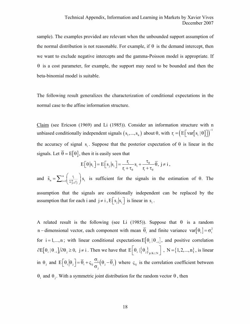
sample). The examples provided are relevant when the unbounded support assumption of

the normal distribution is not reasonable. For example, if θ is the demand intercept, then

we want to exclude negative intercepts and the gamma-Poisson model is appropriate. If

θ is a cost parameter, for example, the support may need to be bounded and then the

beta-binomial model is suitable.

The following result generalizes the characterization of conditional expectations in the

normal case to the affine information structure.

Claim (see Ericson (1969) and Li (1985)). Consider an information structure with n

unbiased conditionally independent signals ( )1 ns ,...,s about θ, with [ ]( ) 1

i ir E var s |−

⎡ ⎤= θ⎣ ⎦

the accuracy of signal is . Suppose that the posterior expectation of θ is linear in the

signals. Let [ ]Eθ = θ , then it is easily seen that

ii j i i

i i

rE s E s s s , j ir r

θ

θ θ

τ⎡ ⎤⎡θ ⎤ = = + θ ≠⎣ ⎦ ⎣ ⎦ + τ + τ,

and n rin ini 1 rjj 1

s s= ∑ =

⎛ ⎞= ⎜ ⎟⎝ ⎠

∑% is sufficient for the signals in the estimation of θ. The

assumption that the signals are conditionally independent can be replaced by the assumption that for each i and j i≠ , j iE s s⎡ ⎤⎣ ⎦ is linear in is .

A related result is the following (see Li (1985)). Suppose that θ is a random

−n dimensional vector, each component with mean iθ and finite variance [ ] 2i ivar θ = σ

for i 1,..., n= ; with linear conditional expectations [ ]i iE | −θ θ , and positive correlation

[ ]i i jE | 0, j i−∂ θ θ ∂θ ≥ ≠ . Then we have that i j j K NE |

∈ ⊂⎡ ⎤θ θ⎣ ⎦

, N 1,2,..., n= , is linear

in jθ and ( )ii j i ij j j

j

E σ⎡ ⎤θ θ = θ + ς θ − θ⎣ ⎦ σ where ijς is the correlation coefficient between

iθ and jθ . With a symmetric joint distribution for the random vector θ , then


19

( )i j jj K Nj K

E | ( )1 k 1∈ ⊂

∈

ς⎡ ⎤θ θ = θ + θ − θ⎣ ⎦ + − ς ∑

where θ is the common mean, ς the correlation coefficient, and k the cardinality of K .

2.3 Common and private values models

In the interaction models we consider in the text there is a set of agents which is finite,

countable, or a continuum (see Section 3 that deals with Nash equilibrium). All agents

have the same prior distribution over the uncertain parameters (the state of the world) and

in most instances this prior coincides with nature’s distribution. Agent i receives private

information about the state of the world and, since he knows how the private information

has been generated, can update in a Bayesian way. Agent i also knows how the private

information of other agents is generated but not the realization of the signals of others,

neither of the state of the world. The information structure is supposed to be common

knowledge, that is, everyone knows the structure, knows that everyone knows the

structure, and so on ad infinitum.

The workhorse model for the analysis in the book is the normal model (or the generalized

affine information structure). We present now a general framework of information

structure for interacting agents encompassing common and private value uncertainty

cases.

Assume the vector of random variables ( )1 n,...,θ θ is jointly normally distributed with

[ ] [ ] 2i iE , var θθ = θ θ = σ and 2

i jcov , , j i, 0 1θ⎡ ⎤θ θ = ςσ ≠ ≤ ς ≤⎣ ⎦ . Agent i receives a signal

i i is = θ + ε where ( )i

2i ~ N 0, εε σ and i jcov , 0⎡ ⎤ε ε =⎣ ⎦ . Signals can range from perfect

(i

2 0εσ = or infinite precision) to pure noise ( ∞=σε2

i or zero precision). The precision of

signal is is given by ( )i i

12 −

ε ετ = σ . It follows that the average parameter ( )nn ii 1

n=

θ ≡ θ∑%


20

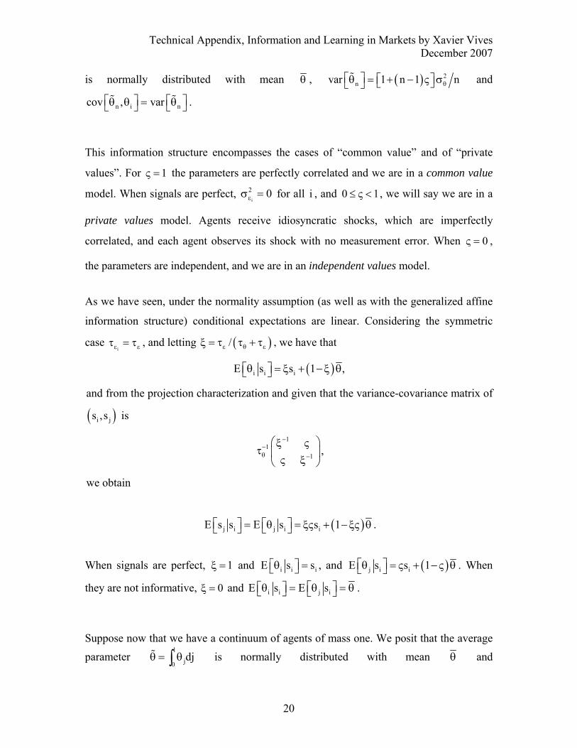
is normally distributed with mean θ , ( ) 2nvar 1 n 1 nθ⎡ ⎤θ = + − ς σ⎡ ⎤⎣ ⎦⎣ ⎦% and

n i ncov , var⎡ ⎤ ⎡ ⎤θ θ = θ⎣ ⎦ ⎣ ⎦% % .

This information structure encompasses the cases of “common value” and of “private

values”. For 1ς = the parameters are perfectly correlated and we are in a common value

model. When signals are perfect, 02i

=σε for all i , and 0 1≤ ς < , we will say we are in a

private values model. Agents receive idiosyncratic shocks, which are imperfectly

correlated, and each agent observes its shock with no measurement error. When 0ς = ,

the parameters are independent, and we are in an independent values model.

As we have seen, under the normality assumption (as well as with the generalized affine

information structure) conditional expectations are linear. Considering the symmetric

case iε ετ = τ , and letting ( )/ε θ εξ = τ τ + τ , we have that

( )i i iE s s 1 ,⎡θ ⎤ = ξ + − ξ θ⎣ ⎦

and from the projection characterization and given that the variance-covariance matrix of

( )i js ,s is

11

1

−−θ −

⎛ ⎞ξ ςτ ⎜ ⎟

ς ξ⎝ ⎠,

we obtain

( )j i j i iE s s E s s 1⎡ ⎤ ⎡ ⎤= θ = ξς + − ξς θ⎣ ⎦ ⎣ ⎦ .

When signals are perfect, 1ξ = and i i iE s s⎡θ ⎤ =⎣ ⎦ , and ( )j i iE s s 1⎡ ⎤θ = ς + − ς θ⎣ ⎦ . When

they are not informative, 0ξ = and i i j iE s E s⎡ ⎤⎡θ ⎤ = θ = θ⎣ ⎦ ⎣ ⎦ .

Suppose now that we have a continuum of agents of mass one. We posit that the average parameter

1

j0djθ = θ∫% is normally distributed with mean θ and


21

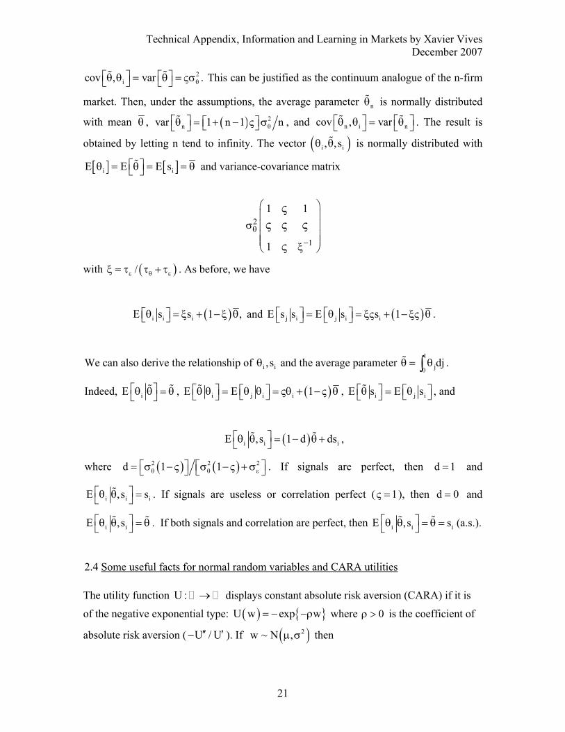
2icov , var θ⎡ ⎤ ⎡ ⎤θ θ = θ = ςσ⎣ ⎦ ⎣ ⎦

% % . This can be justified as the continuum analogue of the n-firm

market. Then, under the assumptions, the average parameter nθ% is normally distributed

with mean θ , ( ) 2nvar 1 n 1 nθ⎡ ⎤θ = + − ς σ⎡ ⎤⎣ ⎦⎣ ⎦% , and n i ncov , var⎡ ⎤ ⎡ ⎤θ θ = θ⎣ ⎦ ⎣ ⎦

% % . The result is

obtained by letting n tend to infinity. The vector ( )i i, ,sθ θ% is normally distributed with

[ ] [ ]i iE E E s⎡ ⎤θ = θ = = θ⎣ ⎦% and variance-covariance matrix

2

1

1 1

1

θ

−

⎛ ⎞⎜ ⎟

σ ⎜ ⎟⎜ ⎟⎜ ⎟ξ⎝ ⎠

ςς ς ς

ς

with ( )/ε θ εξ = τ τ + τ . As before, we have

( )i i iE s s 1 ,⎡θ ⎤ = ξ + − ξ θ⎣ ⎦ and ( )j i j i iE s s E s s 1⎡ ⎤ ⎡ ⎤= θ = ξς + − ξς θ⎣ ⎦ ⎣ ⎦ .

We can also derive the relationship of i i, sθ and the average parameter 1

j0djθ = θ∫% .

Indeed, iE ⎡ ⎤θ θ = θ⎣ ⎦% % , ( )i j i iE E 1⎡ ⎤ ⎡ ⎤θ θ = θ θ = ςθ + − ς θ⎣ ⎦⎣ ⎦

% , i j iE s E s⎡ ⎤ ⎡ ⎤θ = θ⎣ ⎦⎣ ⎦% , and

( )i i iE ,s 1 d ds⎡ ⎤θ θ = − θ +⎣ ⎦% % ,

where ( ) ( )2 2 2d 1 1θ θ ε⎡ ⎤ ⎡ ⎤= σ − ς σ − ς + σ⎣ ⎦ ⎣ ⎦ . If signals are perfect, then d 1= and

i i iE ,s s⎡ ⎤θ θ =⎣ ⎦% . If signals are useless or correlation perfect ( 1ς = ), then d 0= and

i iE ,s⎡ ⎤θ θ = θ⎣ ⎦% % . If both signals and correlation are perfect, then i i iE ,s s⎡ ⎤θ θ = θ =⎣ ⎦

% % (a.s.).

2.4 Some useful facts for normal random variables and CARA utilities

The utility function U : → displays constant absolute risk aversion (CARA) if it is

of the negative exponential type: ( ) U w exp w= − −ρ where 0ρ > is the coefficient of

absolute risk aversion ( U / U′′ ′− ). If ( )2w ~ N ,µ σ then


22

( ) 2E exp w exp / 2− −ρ = − −ρ µ − ρσ⎡ ⎤⎣ ⎦ . More in general we have the following result.

(See Danthine and Moresi (1993) for a proof).

Result. Let the n-dimensional random vector z be normally distributed with mean 0 and

variance-covariance matrix Σ and w c b 'z z 'Az= + + , where c∈ , nb ∈ and A is a

n n× matrix. If the matrix 1 2 A−Σ + ρ is positive definite and 0ρ > , then

( ) ( )( ) ( ) 111/ 21/ 2 1

b ' 2 A bE exp w det det 2 A exp c

2

−−−− −

⎧ ⎫⎡ ⎤ρ Σ + ρ⎪ ⎪⎢ ⎥− −ρ = − Σ Σ + ρ −ρ −⎡ ⎤ ⎨ ⎬⎣ ⎦ ⎢ ⎥⎪ ⎪⎣ ⎦⎩ ⎭

.

A corollary of the result (see Demange and Laroque (1995) for a direct proof) is the following: If ( )2

xx N x,∼ σ , ( )2yy N y,∼ σ and [ ] xycov x y, = σ , then

( )22

xy2 x22yy

y1E exp x y exp x .2 1 21 2

⎧ ⎫+ σσ⎪ ⎪⎡ ⎤− = + −⎨ ⎬⎣ ⎦ + σ+ σ ⎪ ⎪⎩ ⎭

This follows letting 2c x y= − + , 1

b2y−⎛ ⎞

= ⎜ ⎟⎝ ⎠

, 0 0

A0 1

⎛ ⎞= ⎜ ⎟

⎝ ⎠, 1ρ = and

x xz

y y−⎛ ⎞

= ⎜ ⎟−⎝ ⎠. We have

then that 1 2 A−Σ + ρ is positive definite since 2y1 2 0+ σ > :

( ) ( )211 x xy1 2

y 2xy y

2det2A 1 2

−−− ⎡ ⎤σ + Σ σ⎡ ⎤Σ + = + σ ⎢ ⎥⎣ ⎦ σ σ⎢ ⎥⎣ ⎦

and ( ) ( )

2y1 1 2

det 2Adet

− + σΣ + =

Σ.

Furthermore, if x y 0= = then, for any 0ρ ≥ and if x y xy1ρσ σ < + ρσ we have that

( )1/ 22 2 2 2

xy x yE exp xy 1−

⎡ ⎤−ρ = + ρσ − ρ σ σ⎡ ⎤⎣ ⎦ ⎢ ⎥⎣ ⎦.

This follows letting 0 1/ 2

A1/ 2 0

⎛ ⎞= ⎜ ⎟

⎝ ⎠ ,

0b

0⎛ ⎞

= ⎜ ⎟⎝ ⎠

, and c 0= . Then 1 2 A−Σ + ρ is positive

definite if x y xy1ρσ σ < + ρσ . We have that ( )( ) ( ) 1/ 21/ 2 2 2 2x y xydet

−−Σ = σ σ − σ and


23

( ) ( )( )

( )( )

( )( )

1/ 222 21/ 2 x y xy1

2

1/ 221/ 2 2 2 22xy x yxy

detdet 2 A

det

11 2 detdet det

−

−−

−−

⎡ ⎤σ σ − σ − ρ Σ⎢ ⎥⎡ ⎤Σ + ρ =⎣ ⎦ ⎢ ⎥Σ⎡ ⎤⎣ ⎦⎣ ⎦

⎡ ⎤+ ρσ − ρ σ σ⎡ ⎤+ σ ρ − ρ Σ ⎢ ⎥= =⎢ ⎥ ⎢ ⎥Σ Σ⎢ ⎥⎣ ⎦ ⎣ ⎦

.

Therefore,

( ) ( )( ) ( )1/ 2 1/ 22 21/ 2 2 2 2 2 2

x y xy xy x yE exp xy det det 1− −− ⎡ ⎤ ⎡ ⎤−ρ = Σ σ σ − σ − ρ Σ = + ρσ − ρ σ σ⎡ ⎤ ⎡ ⎤⎣ ⎦ ⎣ ⎦ ⎢ ⎥ ⎢ ⎥⎣ ⎦ ⎣ ⎦

.

3. Convergence concepts and results

In this section we state definitions and main results on convergence of random variables

(3.1); rates of convergence (3.2); and martingales and Bayesian learning (3.3). General

references for this section are Spanos (1993, 2000), De Groot (1970), Ash (1972), Chung

(1974), Billingsley (1979), Grimmet and Stirzaker (2001), and Jacod and Protter (2003).

3.1 Convergence of random variables

There are several convergence modes for random variables (see Spanos (1993), ch. 10 for

example).

Definition: Let 1 2 3x, x , x , x ,... be random variables on the probability space ( Ω ,E , P).

We say that i) nx converges to x almost surely (a.s.) and write a.s.

nx x⎯⎯→ if

( ) ( )( )n nP : lim x x 1→∞ω∈Ω ω → ω = ;

ii) nx converges to x in probability and write pnx x⎯⎯→ if, for every fixed

0ε >

( )n nlim P x x 0→∞ − > ε = ;


24

iii) nx converges to x in r th mean (or in rL ), r 1≥ , and write rnx x⎯⎯→ , if

rnE x⎡ ⎤ < ∞⎣ ⎦ for all n and

rn nlim E x x 0→∞

⎡ ⎤− =⎣ ⎦ ;

iv) nx with (cumulative) distribution functions nF converges to x with

(cumulative) distribution function F in distribution (or in law) and write L

nx x⎯⎯→ if, for each continuity point y of F ,

( ) ( )n nlim F y F y→∞ = .

For our purposes it is usually sufficient to consider convergence in the second moment or

mean square. The conditions for convergence in mean square are easy to verify. The

following relationships can be shown to hold:

i) If a.s.nx x⎯⎯→ , then p

nx x⎯⎯→ .

ii) If rnx x⎯⎯→ , then p

nx x⎯⎯→ .

iii) If pnx x⎯⎯→ , then L

nx x⎯⎯→ .

iv) If r t≥ then rnx x⎯⎯→ implies that t

nx x⎯⎯→ .

Two very useful results on the convergence of sums of random variables are the law of

large numbers and the central limit theorem.

Strong Law of Large Numbers (SLLN). Let nx be a sequence of independent random

variables with finite mean [ ]iE x < ∞ and variance [ ]ivar x < ∞ for all i. If

[ ]2kk 1

k var x∞ −=

< ∞∑ then [ ]( )n a.s.i ii 1

1 x E x 0n =

− ⎯⎯→∑ . For the case of identically

distributed random variables there is a stronger result which only requires finite first moments (Khinchine’s version of the SLLN). Let nx be a sequence of i.i.d. random

variables with common finite mean µ < ∞ , then n a.s.ii 1

1 xn =

⎯⎯→µ∑ .


25

In the text we work often with a continuum of agents and we want to invoke the SLLN. A well known potential technical difficulty is that given a process ( ) [ ]i i 0,1

q∈

of independent

random variables, the realizations of the process need not be measurable and therefore the

Lebesgue integral 1

i0q di∫ is not well defined (see Judd (1985) for the measure-theoretical

issues involved). Note however that if [ ]iE q 0= and [ ]ivar q are uniformly bounded,

then for every sequence ki of different indices extracted from [ ]0,1 , the Strong Law of

Large Numbers applied to kiq yields

k

n a.s.ik 1

1 q 0n =

⎯⎯→∑ (note that if

kivar q M⎡ ⎤ ≤ < ∞⎣ ⎦ then k

2 2ik 1 k 1

k var q M k∞ ∞− −= =

⎡ ⎤ ≤ < ∞⎣ ⎦∑ ∑ ). However, as pointed out

by Allen (1982) and Feldman and Gilles (1985), with a continuum of agents there are

countable families of sets for which a law of large numbers can not hold.

In the text when we work with a continuum of agents, we make the convention that the

Strong Law of Large Numbers holds for a continuum of independent random variables with uniformly bounded variances. Suppose thus that ( ) [ ]i i 0,1

q∈

is a process of

independent random variables with mean [ ]iE q 0= and uniformly bounded variances

[ ]ivar q . Then we let 1

i0q di 0=∫ almost surely (a.s.). This convention will be used, taking

as given the usual linearity property of integral (see Admati (1985)). For example, assume a continuum of agents indexed in the unit interval [ ]0,1 and endowed with the

Lebesgue measure. Each agent i receives a signal i is = θ + ε , where [ ]E 0ε = and θ is

randomly distributed with finite variance. If signals have uniformly bounded variance, we

will write

( ) ( )1 1 1

i i i0 0 0s di di di a.s.= θ + ε = θ + ε = θ∫ ∫ ∫ ,

using the linearity of the integral and our convention.

The case of different means can also be dealt with. Suppose that ( ) [ ]i i 0,1

q∈

is a process of

independent random variables with means [ ]iE q and uniformly bounded


26

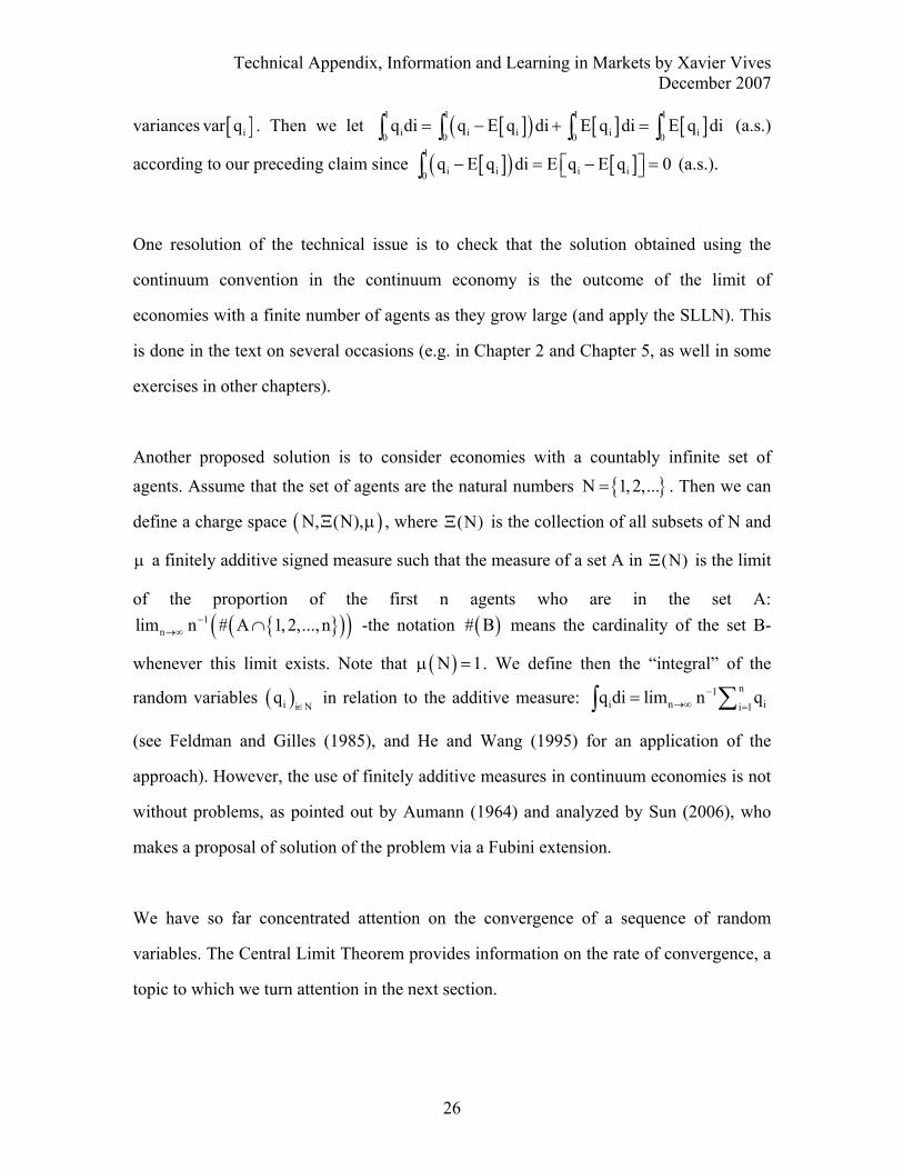
variances [ ]ivar q . Then we let [ ]( ) [ ] [ ]1 1 1 1

i i i i i0 0 0 0q di q E q di E q di E q di= − + =∫ ∫ ∫ ∫ (a.s.)

according to our preceding claim since [ ]( ) [ ]1

i i i i0q E q di E q E q 0⎡ ⎤− = − =⎣ ⎦∫ (a.s.).

One resolution of the technical issue is to check that the solution obtained using the

continuum convention in the continuum economy is the outcome of the limit of

economies with a finite number of agents as they grow large (and apply the SLLN). This

is done in the text on several occasions (e.g. in Chapter 2 and Chapter 5, as well in some

exercises in other chapters).

Another proposed solution is to consider economies with a countably infinite set of agents. Assume that the set of agents are the natural numbers N 1,2,...= . Then we can

define a charge space ( )N, (N),Ξ µ , where (N)Ξ is the collection of all subsets of N and

µ a finitely additive signed measure such that the measure of a set A in (N)Ξ is the limit

of the proportion of the first n agents who are in the set A: ( )( )1

nlim n # A 1,2,..., n−→∞ ∩ -the notation ( )# B means the cardinality of the set B-

whenever this limit exists. Note that ( )N 1µ = . We define then the “integral” of the

random variables ( )i i Nq

∈ in relation to the additive measure: n1

i n ii 1q di lim n q−

→∞ == ∑∫

(see Feldman and Gilles (1985), and He and Wang (1995) for an application of the

approach). However, the use of finitely additive measures in continuum economies is not

without problems, as pointed out by Aumann (1964) and analyzed by Sun (2006), who

makes a proposal of solution of the problem via a Fubini extension.

We have so far concentrated attention on the convergence of a sequence of random

variables. The Central Limit Theorem provides information on the rate of convergence, a

topic to which we turn attention in the next section.


27

Central limit theorem (CLT). Let nx be a sequence of i.i.d. random variables with

finite mean [ ]iE x = µ < ∞ and variance [ ] 2ivar x = σ < ∞ . Let

nii 1

n

x ny

n=

− µ=

σ∑ , then

ny converges in distribution to y , Lny y⎯⎯→ , where ( )y ~ N 0,1 .

The CLT implies that n

ii 1x

nn=

⎛ ⎞⎜ ⎟− µ⎜ ⎟⎝ ⎠

∑ converges in distribution to ( )2,0N σ and we can

identify 1/ n as the rate at which n

ii 1x

n= − µ∑ converges to 0 (a.s. according to the

SLLN).

3.2 Rates of convergence We say that the sequence of real numbers nb is at most of order ( )nφ , for some

function ( )φ ⋅ with integer domain, and we write ( )( )nO φ , if there is a nonzero constant

2k such that ( )n 2b k n≤ φ for on n≥ for some appropriate on . We say that the sequence

of real numbers nb is of the order ( )nφ , for some function ( )φ ⋅ with integer domain,

if there are nonzero constants 1k , 2k such that ( ) ( )1 n 2k n b k nφ ≤ ≤ φ for on n≥ for

some appropriate on A somewhat more restrictive definition, good enough for our

purposes, is to say that nb is of the order ( )nφ whenever ( )n nb / n kφ ⎯⎯→ as n tends

to ∞ for some nonzero constant k. Suppose that n nb 0⎯⎯→ and nb is of the order

( )nφ then we say also that nb converges to 0 at the rate ( )nφ . We will often use

( )n nυφ = , with υ a real number. Other examples are the logarithmic ( ) ( )n log nφ = or

the exponential ( ) nnφ = κ with κ > 1.

For sequences of random variables things are a little more complex and we have to work

with the appropriate convergence concepts by analogy. For example, we will say that the


28

sequence of random variables ty converges to 0 almost surely (at least) at an

exponential rate if there is a constant κ > 1 such that nn ny 0κ ⎯⎯→ (almost surely).

With rth mean convergence we can apply the rate of convergence definition for real

numbers easily. We will say that the sequence of random variables ny converges in

mean square to zero at the rate r1/ n (or that ny is of the order r1/ n ) if

2nE y⎡ ⎤⎣ ⎦ converges to zero at the rate r1/ n (i.e. 2

nE y⎡ ⎤⎣ ⎦ is of the order r1/ n ).

Given that 2

nE y⎡ ⎤⎣ ⎦ = [ ]( )2

nE y + [ ]nvar y , a sequence ny such that [ ]nE y = 0 and

[ ]nvar y is of the order of 1/ n , converges to zero at the rate 1/ n . This is the typical

convergence rate for the sample mean to converge to the population mean associated with the law of large numbers. For example, if the random variables nx are i.i.d. with finite

mean [ ]iE x = µ < ∞ and variance [ ] 2ivar x = σ < ∞ , then n r 21

n ii 1y n x 0=−

== − µ ⎯⎯→∑

(i.e. in mean square) at the rate 1/ n because n1ii 1

E n x−=

⎡ ⎤− µ⎣ ⎦∑ = 0 and n1

ii 1var n x−

=⎡ ⎤⎣ ⎦∑ = 2 / nσ .

A more refined measure of convergence speed for a given convergence rate is provided

by the asymptotic variance. Suppose that ny is such that [ ]nE y 0= and

[ ]2n nE y var y⎡ ⎤ =⎣ ⎦ converges to 0 at the rate r1/ n for some r > 0. Then, the asymptotic

variance is given by the constant AV = [ ]rn nAV lim n var y→∞= . A higher asymptotic

variance means that the speed of convergence is slower. It is worth noting that ( )rnn y

converges in distribution to ( )N 0, AV . Indeed, a normal random variable is characterized

by mean and variance and we have that ( ) [ ]r rn nvar n y n var y⎡ ⎤ =⎣ ⎦

tends to AV as n

tends to infinity.


29

Often normality is not needed for the result. Indeed, from the CLT we have that if the

random variables nx are i.i.d. with finite mean [ ]iE x = µ < ∞ and variance

[ ] 2ivar x = σ < ∞ , then ( )nn y , where n1

n ii 1y n x−

== − µ∑ , converges in distribution to

( )2N 0,σ . From the SLLN we have also that a.sny 0⎯⎯→ .

All this suggests that we can say, alternatively, that ny converges to zero almost surely

at the rate r1/ n if a.sny 0⎯⎯→ and ( ) ( )Lr

nn y N 0,AV⎯⎯→ for some positive

constant AV. In this book we will say that the sequence of random variables ny

converges to 0 at the rate n−υ , with υ > 0, if n ny 0⎯⎯→ (a.s. or in mean square) and

( )Ln nn y N 0, AVυ ⎯⎯→ for some positive constant AV.

As an example with general distributions and linear prediction consider the following

statistical estimation problem. An unknown parameter θ with finite variance is to be estimated from the observations n

1 nz z ,..., z= where t t tz a u= θ + , with ta known

constants, t = 1,.., n, and tu are i.i.d. random variables with zero mean and finite

variance 2uσ . We know (see the last paragraph in Section 2.1) that with finite second

moments ( )2 2u,θσ σ the unique best (mean squared error) linear predictor of θ based on nz

is given by the same expression as under normality:

( )nnu k k nk 1

E z a z /θ =⎡ ⎤θ = τ θ + τ τ⎣ ⎦ ∑

where n 2n u kk 1

aθ =τ = τ + τ ∑ . Denote by ny the OLS estimate of θ regressing tz on ta ,

that is n1n n t tt=1

y A a z−= ∑ , n 2n tt=1

A a= ∑ . Then ( )nu n n nE z A y /θ⎡ ⎤θ = τ θ + τ τ⎣ ⎦ .

The following result provides conditions under which ny (or nE z⎡ ⎤θ⎣ ⎦ ) converge to θ a.s.

as n tends infinity and characterizes the rate of convergence. It uses SLLN and CLT type

arguments.


30

Result: Let n1n n t tt=1

y A a z−= ∑ , n 2

n tt=1A a= ∑ be the OLS estimator of the unknown

parameter θ with finite variance based on the data t t tz a u= θ + , with ta known constants, t = 1,.., n, and tu i.i.d. random variables with zero mean and finite variance

2uσ . Suppose

n 2n u kk 1

aθ =τ = τ + τ ∑ is of the order nυ , and ta is a sequence of order

t− κ for some constants υ > 0 and κ ≥ 0 such that 1/ 2υ + κ > . Let n nA lim n−υ∞ →∞τ = τ .

Then

(i) a.s.ny ⎯⎯→θ , and

(ii) ( ) ( )( )1Lnn y N 0, A −υ

∞− θ ⎯⎯→ τ .

Proof: See Proof of Lemma 3.2 in Vives (1993).

3.3 Martingales and Bayesian learning

A stochastic process is an indexed collection of random variables t t Tx

∈ defined on the

same probability space ( Ω ,E , P).

Suppose that an agent receives a sequence of signals tz about an unknown parameter

θ . The agent has a prior on θ and he knows the likelihood distribution of the signals for

any given value of θ . We would like to know properties of the (Bayesian) posterior

probability assessment of the agent as more signals accumulate. Given a sequence of

random variables t t 0z

≥ let t

0 1 tz z , z ,..., z= denote the history of the process up to t.

Information accumulation is represented by a filtration (an increasing sequence of sub-

sigma fields of E ). This is the increasing sequence of sigma fields ( )t 1z −σ generated by

the random variables t 10 1 t 1z z , z ,..., z−

−= , t = 1, 2, … . The agent does not forget once

he has learned.

Consider a sequence of random variables t t 0x

≥. Recall that when we write t 1

tE x | z −⎡ ⎤⎣ ⎦

we mean the conditional expectation of tx given the -fieldσ generated by the random


31

variables t 10 1 t 1z z , z ,..., z−

−= : ( )t 1tE x | z −⎡ ⎤σ⎣ ⎦ . This conditional expectation is a random

variable ( )t 1z −σ -measurable (see Spanos (2000, Section 7.3) and Section 6.2 in Ash

(1972)).

Consider the sequence of random variables t t 0x

≥on the probability space ( Ω ,E , P) and

let t t 0≥E be an increasing sequence of fieldsσ − in E (i.e. t t 1+⊂E E ). The sequence

t t 0x

≥is a martingale relative to the fieldsσ − t t 0≥

E if tx is tE -measurable,

tE x⎡ ⎤ < ∞⎣ ⎦ , and [ ]t t 1 t 1E x | x− −=E with probability 1 (a.s.).

We say that the sequence of random variables t t 0x

≥ is a martingale relative to the

history tz if for all t: tE x⎡ ⎤ < ∞⎣ ⎦ and t 1t t 1E x | z x−

−⎡ ⎤ =⎣ ⎦ (a.s.).

We will say also that the stochastic process or sequence of random variables t t 0x

≥ is a

martingale if for all t: tE x⎡ ⎤ < ∞⎣ ⎦ and t 1t t 1E x | x x−

−⎡ ⎤ =⎣ ⎦ (a.s.) (i.e. t t 0x

≥ is martingale

relative to the increasing sigma fields ( )t 1x −σ ). Note [ ]t 1t t 1E x x x−

−= implies that

[ ] [ ]t 1t t t 1 t 1E x x E x x x−

− −= = . The martingale property means that the conditional

expectation of the present tx given the history of the process t 1x − is just the immediate

past t 1x − . It also means that the conditional expectation of the future t kx , k 1+ ≥ , given

the history of the process up to the present tx is just the present tx : tt k tE x | x x+⎡ ⎤ =⎣ ⎦

(since the sigma fields ( )txσ are increasing). Let t t t 1x x x −∆ = − (with 0 0x x∆ = ) we

have then that [ ]tE x 0∆ = and t 1tE x x 0−⎡ ⎤∆ =⎣ ⎦ for t 1≥ . It is worth noting that since

kk tt 0

x x=

= ∆∑ we have that ( ) ( )0 t 0 tx ,..., x x ,..., xσ = σ ∆ ∆ .

Some important facts about martingales are the following.


32

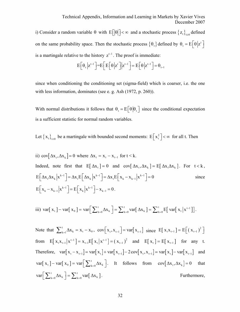
i) Consider a random variable θ with E ⎡ θ ⎤ < ∞⎣ ⎦ and a stochastic process t t 0z

≥defined

on the same probability space. Then the stochastic process tθ defined by tt E z⎡ ⎤θ = θ⎣ ⎦

is a martingale relative to the history t 1z − . The proof is immediate:

t 1 t t 1 t 1t t 1E z =E E z z E z− − −

−⎡ ⎤⎡ ⎤ ⎡ ⎤ ⎡ ⎤θ θ = θ = θ⎣ ⎦ ⎣ ⎦ ⎣ ⎦⎣ ⎦

since when conditioning the conditioning set (sigma-field) which is coarser, i.e. the one

with less information, dominates (see e. g. Ash (1972, p. 260)).

With normal distributions it follows that t tEθ = ⎡θ θ ⎤⎣ ⎦ since the conditional expectation

is a sufficient statistic for normal random variables.

Let t t 0x

≥ be a martingale with bounded second moments: 2

tE x⎡ ⎤ < ∞⎣ ⎦ for all t. Then

ii) [ ]t kcov x , x 0∆ ∆ = where t t t 1x x x −∆ = − for t < k.

Indeed, note first that [ ]tE x 0∆ = and [ ] [ ]t k t kcov x , x E x x∆ ∆ = ∆ ∆ . For t k< ,

k 1 k 1 k 1t k t k t k k 1E x x x x E x x x E x x x 0− − −

−⎡ ⎤ ⎡ ⎤ ⎡ ⎤∆ ∆ = ∆ ∆ = ∆ − =⎣ ⎦ ⎣ ⎦ ⎣ ⎦ since

k 1 k 1k k 1 k k 1E x x x E x x x 0− −

− −⎡ ⎤ ⎡ ⎤− = − =⎣ ⎦ ⎣ ⎦ .

iii) [ ] [ ] [ ] [ ][ ]t t t t 1t 0 k k tk 0 k 0 k 0

var x var x var x var x E var x x −= = =

⎡ ⎤− = ∆ = ∆ =⎣ ⎦∑ ∑ ∑ .

Note that tk t 0k 1

x x x=

∆ = −∑ , [ ]t t 1 t 1cov x , x var x− −⎡ ⎤ =⎣ ⎦ since [ ] ( )2t t 1 t 1E x x E x− −⎡ ⎤= ⎣ ⎦

from [ ] [ ] ( )2t 1 t 1t t 1 t 1 t t 1E x x x x E x x x− −

− − −= = and [ ] [ ]t t 1E x E x −= for any t.

Therefore, [ ] [ ] [ ] [ ] [ ] [ ]t t 1 t t 1 t t 1 t t 1var x x var x var x 2cov x , x var x var x− − − −− = + − = − and

[ ] [ ] tt 0 kk 0

var x var x var x=

⎡ ⎤− = ∆⎣ ⎦∑ . It follows from [ ]t kcov x , x 0∆ ∆ = that

[ ]t tk kk 0 k 0

var x var x= =

⎡ ⎤∆ = ∆⎣ ⎦∑ ∑ . Furthermore,


33

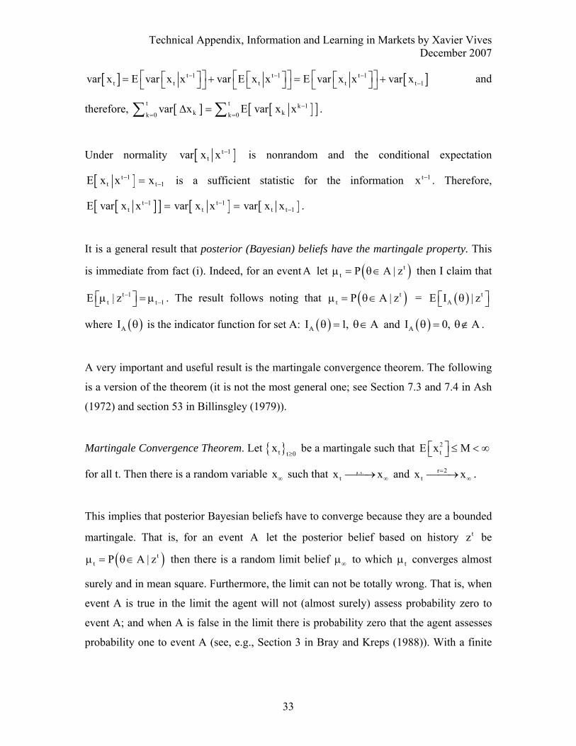
[ ] [ ]t 1 t 1 t 1t t t t t 1var x E var x x var E x x E var x x var x− − −

−⎡ ⎤ ⎡ ⎤ ⎡ ⎤⎡ ⎤ ⎡ ⎤ ⎡ ⎤= + = +⎣ ⎦ ⎣ ⎦ ⎣ ⎦⎣ ⎦ ⎣ ⎦ ⎣ ⎦ and

therefore, [ ] [ ][ ]t t k 1k kk 0 k 0

var x E var x x −= =

∆ =∑ ∑ .

Under normality [ ]t 1tvar x x − is nonrandom and the conditional expectation

[ ]t 1t t 1E x x x−

−= is a sufficient statistic for the information t 1x − . Therefore,

[ ][ ] [ ] [ ]t 1 t 1t t t t 1E var x x var x x var x x− −

−= = .

It is a general result that posterior (Bayesian) beliefs have the martingale property. This

is immediate from fact (i). Indeed, for an event A let ( )tt P A | zµ = θ∈ then I claim that

t 1t t 1E | z −

−⎡ ⎤µ = µ⎣ ⎦ . The result follows noting that ( )tt P A | zµ = θ∈ = ( ) t

AE I | z⎡ ⎤θ⎣ ⎦

where ( )AI θ is the indicator function for set A: ( )AI 1, Aθ = θ∈ and ( )AI 0, Aθ = θ∉ .

A very important and useful result is the martingale convergence theorem. The following

is a version of the theorem (it is not the most general one; see Section 7.3 and 7.4 in Ash

(1972) and section 53 in Billinsgley (1979)).

Martingale Convergence Theorem. Let t t 0x

≥ be a martingale such that 2

tE x M⎡ ⎤ ≤ < ∞⎣ ⎦

for all t. Then there is a random variable x∞ such that a.s.tx x∞⎯⎯→ and r 2

tx x=∞⎯⎯→ .

This implies that posterior Bayesian beliefs have to converge because they are a bounded

martingale. That is, for an event A let the posterior belief based on history tz be

( )tt P A | zµ = θ∈ then there is a random limit belief ∞µ to which tµ converges almost

surely and in mean square. Furthermore, the limit can not be totally wrong. That is, when

event A is true in the limit the agent will not (almost surely) assess probability zero to

event A; and when A is false in the limit there is probability zero that the agent assesses

probability one to event A (see, e.g., Section 3 in Bray and Kreps (1988)). With a finite


34

number of states (with prior positive weight), and given a true state, this implies that if

the Bayesian updating process converges to a point, it must converge to the truth.

A corollary of the result is that the sequence of (cumulative) conditional distributions

based on history tz converges in law to a limit conditional distribution.

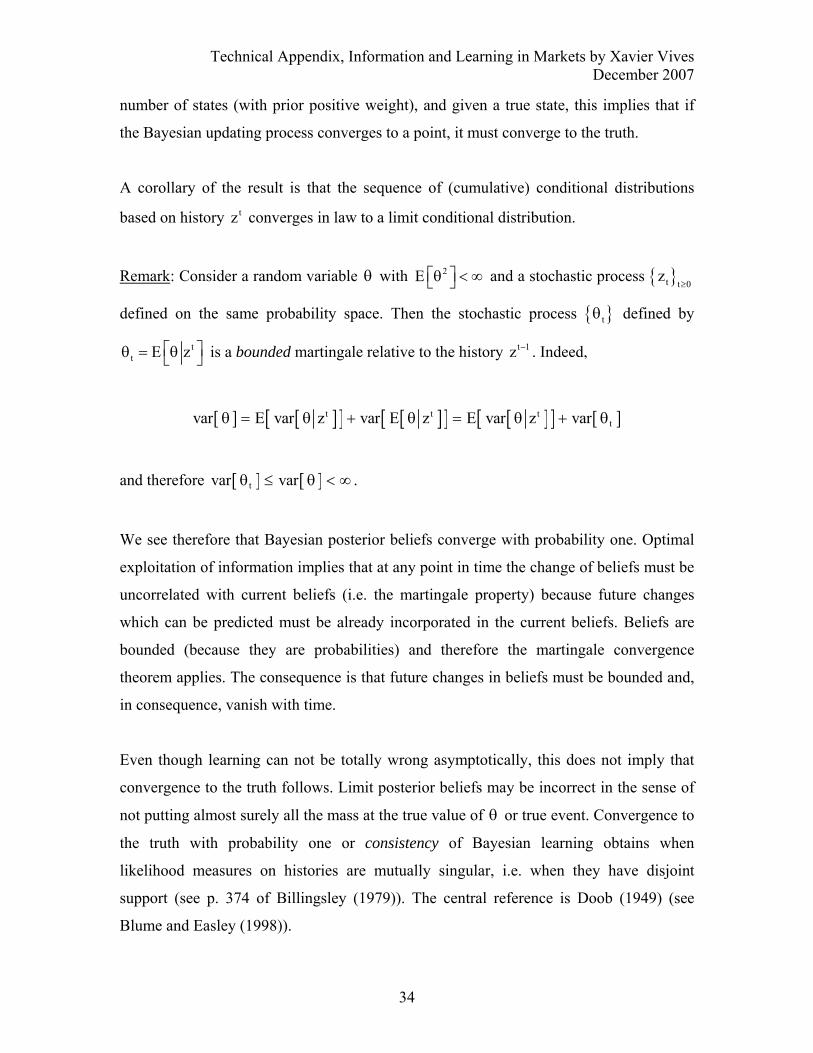
Remark: Consider a random variable θ with 2E ⎡ ⎤θ < ∞⎣ ⎦ and a stochastic process t t 0z

≥

defined on the same probability space. Then the stochastic process tθ defined by

tt E z⎡ ⎤θ = θ⎣ ⎦ is a bounded martingale relative to the history t 1z − . Indeed,

[ ] [ ][ ] [ ][ ] [ ][ ] [ ]t t ttvar E var z var E z E var z varθ = θ + θ = θ + θ

and therefore [ ] [ ]tvar varθ ≤ θ < ∞ .

We see therefore that Bayesian posterior beliefs converge with probability one. Optimal

exploitation of information implies that at any point in time the change of beliefs must be

uncorrelated with current beliefs (i.e. the martingale property) because future changes

which can be predicted must be already incorporated in the current beliefs. Beliefs are

bounded (because they are probabilities) and therefore the martingale convergence

theorem applies. The consequence is that future changes in beliefs must be bounded and,

in consequence, vanish with time.

Even though learning can not be totally wrong asymptotically, this does not imply that

convergence to the truth follows. Limit posterior beliefs may be incorrect in the sense of

not putting almost surely all the mass at the true value of θ or true event. Convergence to

the truth with probability one or consistency of Bayesian learning obtains when

likelihood measures on histories are mutually singular, i.e. when they have disjoint

support (see p. 374 of Billingsley (1979)). The central reference is Doob (1949) (see

Blume and Easley (1998)).


35

In general, convergence to the truth requires that prior beliefs be consistent with the true

model. A Bayesian agent will never learn the truth if he puts zero weight on the true

value of the parameter to start with. With a finite number of states if the agent attaches

prior positive weight to the true state and the Bayesian updating process converges to a

point, it must converge to the truth. For Bayesian learning to obtain it is not necessary

that the agent knows nature’s probability distribution over the unknown parameter θ .

What is needed, in a world with a finite or countable number of states, is that if a

parameter has positive weight in the true model (nature’s model) then it should have

positive weight also in the subjective prior distribution of the agent. In more technical

terms, and for general distributions, the true distribution must be absolutely continuous

with respect to the prior. This means that if the prior assigns probability zero to an event

then the true model must assign probability zero to the event also (see Blume and Easley

(1998)).

4. Games and Bayesian equilibrium

We start by describing briefly the basics of games in normal form and Nash equilibrium,

including some material on supermodular games (Section 4.1), and move to Nash

equilibrium in games of incomplete information (Bayesian equilibrium) in Section 4.2

Sections 4.3 introduces mechanism design and Section 4.4 perfect Bayesian equilibrium.2

4.1 Games and Nash equilibrium

A game in normal or strategic form describes the possible actions and derived payoffs of

the action profiles for each of a given set of players. It consists of a triplet ( )X, , Nπ ,

where the set of players N can be finite, 1, 2, ..., n , countably infinite, 1, 2, ...,.. , or

a continuum, say the interval [ ]0,1 ; ii NX X

∈= ∏ , where iX is the set of possible actions

2 See Chapter 2 in Vives (1999) for a fuller development of Sections 4.1 and 4.2.


36

(or pure strategies) of player i ; and ( )i i N∈π = π with i : Xπ → the payoff function of

player i . All these elements are common knowledge to the players. That is, every player

knows them and knows that other players know and knows that other players know that

he knows, and so on ad infinitum (see Aumann (1976)).

A game can also be represented in extensive form with a complete specification for each

player of the order of moves, feasible choices, information available when making a

choice and payoff for each possible outcome that follows from the choices made by the

players. A strategy is then a complete contingent plan of action for any possible

distinguishable circumstance that the player may have to act upon.

Each player tries to maximize his payoff by choosing an appropriate strategy in his

strategy set knowing the structure of the game, that is, the strategy spaces and payoffs of

other players. Each player must conjecture the strategies that the rivals are going to use.

In a Nash equilibrium, the conjectures of the players must be correct, and no player must

have an incentive to change his strategy given the choices of rivals. With a finite number

of players denote by ix− the vector ( )1 i 1 i 1 nx , ..., x , x , ..., x− + . A Nash equilibrium is

then a set of strategies ( )* * * *1 2 nx x , x , ..., x= such that ( ) ( )* *

i i i ix x , x−π ≥ π for all

i ix X∈ and for each i.

An example with a continuum of players is the following. Let N = [ ]0,1 (and endow it

with the Lebesgue measure). The payoff to player i is given by ( )i ix , xπ where

1

j0x x dj= ∫ denotes the average action. A Nash equilibrium is then a strategy profile

( )*j j N

x∈

such that ( ) ( )* * *i i i ix , x x , xπ ≥ π for all i ix X∈ and for each i. Note that now an

individual player can not affect the average action.

4.1.1 Dominated strategies and rationalizability.


37

Even in a situation where there is common knowledge of payoffs and rationality of the

players, Nash behavior may not be compelling. A much weaker requirement is for agents

not to play strictly dominated strategies. In the game ( )X, , Nπ a (pure) strategy ix is

strictly dominated by another (pure) strategy iy if for all ix− :

( ) ( )i i i i i ix , x y , x− −π < π . (We could consider similarly domination by a mixed

strategy.) A rational player will not play a strictly dominated strategy. Serially

undominated strategies are those that survive a process of iterated elimination of strictly

dominated strategies. A game is dominance solvable if the set remaining after iterated

elimination of strictly dominated strategies is a singleton. In this case the surviving

strategy profile is a Nash equilibrium. Under the maintained assumption of common

knowledge of payoffs and rationality it is possible to rule out more strategies than by

iterated elimination of strictly dominated strategies. This leads to the set of rationalizable

strategies. A strategy is rationalizable if it is a best response to some beliefs about the

play of opponents. However, since the opponents are also rational, and payoffs are

common knowledge, the beliefs cannot be arbitrary. Nash equilibrium strategies are,

obviously, rationalizable, but in general the rationalizable set is much larger (Bernheim

(1984), and Pearce (1984)).

4.1.2 Supermodular games

A game of strategic complementarities (GSC) is one where the best responses of the

players are increasing in the actions of rivals. The technical concept of supermodular

game (to be shortly defined below) provides sufficient conditions for best responses to be

increasing. Let us start with some definitions.

Consider a partial order in k (for instance, the usual componentwise ordering: x y≤ if

and only if i ix y≤ for all 1 i k≤ ≤ ). A function f : X → , where kX ⊂ is a

rectangle (or “box”) in Euclidean space is supermodular if for all Xy,x ∈ ,

( ) ( ) ( ) ( )f max(x, y) f min(x, y) f x f y+ ≥ + ; f is log-supermodular if it is nonnegative

and its logarithm is supermodular, that is, for all Xy,x ∈ ,


38

( ) ( ) ( ) ( )f max(x, y) f min(x, y) f x f y⋅ ≥ ⋅ . For a function 2f : → , supermodularity

requires that the incremental returns to increasing x, defined by ( ) ( ) ( )H Lh t f x ; t f x ; t≡ −

with H Lx x> must be increasing in t; log-supermodularity of a positive function requires

that the relative returns, ( ) ( )H Lf x ; t f x ; t , are increasing in t.

Let X be as before and T a partially ordered set. The function f : X T× → has

(strictly) increasing differences in its two arguments ( )x,t if ( ) ( )−f x,t f x,t ' is

(strictly) increasing in x for all ≥t t ' , ≠t t ' . Decreasing differences are defined

replacing “increasing” by “decreasing”. The two concepts coincide for functions defined

on a product of ordered sets. If kf : → is twice-continuously differentiable, then f is

supermodular if and only if 2

i j

f 0x x∂

≥∂ ∂

for all x and i ≠ j.

In Euclidean space a supermodular game is one where for each player i the strategy set

iX is a compact rectangle (or “box”), the payoff function iπ is continuous and fulfills

two complementarity properties:

• Supermodularity in own strategies ( iπ is supermodular in ia ): the marginal

payoff to any strategy of player i is increasing in the other strategies of the

player.

• Strategic complementarity in rivals' strategies ( iπ has increasing differences in

( ,i ia a− )): the marginal payoff to any strategy of player i is increasing in any

strategy of any rival player.

In a more general formulation of a supermodular game, strategy spaces and the continuity

requirement can be weakened. In a supermodular game very general strategy spaces can

be allowed. These include indivisibilities as well as functional strategy spaces, such as

those arising in dynamic or Bayesian games. Regularity conditions such as concavity and

restriction to interior solutions can be dispensed with. The application of the theory can


39

be extended by considering increasing transformations of the payoff (which does not

change the equilibrium set of the game). We say that the game is log-supermodular if

iπ is nonnegative and if log iπ fulfills the complementarity conditions.

In a supermodular game:

1. There always exist extremal equilibria: a largest x and a smallest element x of the

equilibrium set. If the game is symmetric the extremal equilibria are symmetric.

2. Multiple equilibria are common. If the game displays positive spillovers (i.e. the

payoff to a player is increasing in the strategies of the other players) then the largest

equilibrium point is the Pareto best equilibrium, and the smallest one the Pareto worst.

3. Simultaneous best-reply dynamics approach the “box” [ ]x, x defined by the smallest

and the largest equilibrium points of the game, and converge monotonically downward

(upward) to an equilibrium starting at any point in the intersection of the upper (lower)

contour sets of the largest (smallest) best replies of the players. The extremal equilibria x

and x correspond to the largest and smallest serially undominated strategies. Therefore, if

the equilibrium is unique then the game is dominance solvable (and globally stable).

4. If ( )i i ix , x ;−π θ has increasing differences in ( )ix ,θ for each i then with an increase

in θ : (i) the largest and smallest equilibrium points increase; and (ii) starting from any

equilibrium, best-reply dynamics lead to a larger equilibrium following the parameter

change.

4.2 Nash equilibrium with incomplete information3

In many instances a player does not know some characteristic (or “type”) of the payoff or

strategy space of other players. For example, a firm may have private information about

demand conditions or may not know the costs of production of the rival (as in Chapters 1

3 See Vives (2005) for a development of the material in this Section.


40

and 2), or an investor may receive a private signal about the fundamental value of the

asset. Those are games of incomplete information. Harsanyi (1967-1968) provided the

fundamental insight to deal with such games.

In a game of incomplete information the characteristics or type of each player are known

to the player but not to the other players. Harsanyi introduces a move of Nature at the

beginning of the game choosing the types of the players. Each player is informed about

his type but not about the types of other players. The type of a player embodies all the

relevant private information in order to make his decisions. Nature’s probability

distribution is typically assumed to be common knowledge among the players. This is the

case of a common prior (If the prior is not common then the beliefs of players will be

inconsistent). Each player has thus imperfect information about the move of the Nature

and by observing his type may update his prior belief on the types of others. A Bayesian

Nash equilibrium is then just a Nash equilibrium of the imperfect information version of

the game. We will refer often to Bayesian equilibrium.

Suppose the set N of players is finite. Let iT be the set of possible types of player i (a

subset of Euclidean space), i i∈t T . The types of the players are drawn from a common

prior distribution F on n

ii 0== ∏T T where 0T represents residual uncertainty not observed

by any player. Let iF be the marginal distribution on iT . Let the action space of player i

be a compact rectangle of Euclidean space iX and his payoff be given by the (measurable

and) bounded function i : Xπ × →T . The (ex post) payoff to player i when the vector

of actions is ( )1 nx x ,..., x= and the realized types 1 n( ,..., )=t t t is thus i (x; )π t .

Action spaces, payoff functions, type sets, and the prior distribution are common

knowledge. A (pure) strategy for player i is a (measurable) function i i i: Xϕ →T which

assigns an action to every possible type of the player. Let Ξi denote the strategy space of

player i and identify two strategies of player i if they are equal iF -almost surely (a.s.). Let


41

1 n( ,..., )ϕ = ϕ ϕ . The expected payoff to player i, when agent j uses strategy jϕ , is given

by ( ) ( )( )i i 1 1 n n( ) ,..., ;⎡ ⎤Π ϕ = Ε π ϕ ϕ⎣ ⎦t t t .

A Bayesian Nash equilibrium (BNE) is a Nash equilibrium of the game where the strategy space of player i is Ξi and his payoff function Πi . Given the strategies ( )jϕ ⋅ ,

ij ≠ , denote by ( )i i− −ϕ t the vector ( ) ( )( )1 1 n n,...,ϕ ϕt t except the thi component. The

expected payoff of player i conditional on it when the other players use strategies i−ϕ

and player i chooses action ix is ( )( )i i i i iE x , ;− −⎡ ⎤π ϕ⎣ ⎦t t t . The profile of strategies ϕ is a

BNE if and only if for every i the action i i ix ( )= ϕ t maximizes over iX the conditional

payoff ( )( )i i i i iE x , ;− −⎡ ⎤π ϕ⎣ ⎦t t t ( iF -a.s. on iT ). The model allows for private values when ( )i ix;π t (e.g. each firm observes his

idiosyncratic shock to costs) or a common value with ( ) ( )i i i jjx ; v x ;π = ∑t t (e.g. each

firm observes one component of a common demand shock) or ( )i 0x;π t (e.g. each firm receives a signal –its type- about a common demand shock).

An example with a continuum of players indexed in the interval [0, 1] would be the following. Let the payoff function of firm i by ( )i ix , x ;π θ% , where ix is the action of the

firm, x% a vector of statistics that characterizes the distribution of the firms’ actions, and

iθ a parameter drawn from a prior distribution. Suppose that player i receives a signal it

about the parameter iθ . As before a strategy for player i is a measurable function ( )iϕ ⋅

from the signal space to the action space of the firm. A set of strategies ( )( ) [ ]i i 0,1∈ϕ ⋅ form

a Bayesian equilibrium if for any player (almost surely)

( ) ( )

i i

*i i z X i i iarg max E z , x ;∈

⎡ ⎤ϕ ∈ π θ⎣ ⎦%t t

where *x% the vector of statistics that characterizes the equilibrium distribution of the

actions of players. In this case player i when optimizing takes as given the equilibrium

statistics since his action can not influence them.


42

4.2.1 The linear-normal model

The linear – normal model, that is, linear-quadratic payoffs with normal distributions for

the uncertain parameters and signals –or distributions that yield affine conditional

expectations, is a workhorse model for both the cases of a finite and a continuum of

players. The information structure has been developed in Section 2.3. The usefulness of

the linear-normal model is that it yields typically a unique linear Bayesian equilibrium.

This equilibrium is the unique one in games (such as Cournot or Bertrand games) where

the strategy space of players is a noncontingent strategy like an output or price. There are

at least two routes to show uniqueness. One is a direct proof (see the proof in a version of

the continuum model in Exercise 7.3 in Chapter 7). The other route is to realize that in

many linear-quadratic games there is a potential or team function the optimization of

which yields the Bayesian-Nash equilibria of the game. If this team optimization problem

has a unique solution then the equilibrium will be unique (this method is introduced in

Vives (1988), see the proof of Proposition 2.1 in Chapter 2 for an n-player model and

Section 8.1 in Vives (1999)). Characterizations of the linear equilibrium in the continuum

model in Cournot or Bertrand environments are found in Section 1.2.4.1 and in the proof

of Proposition 1.3. In models where the strategy space is functional, a supply or a demand

function like in rational expectations models, then typically we can only show that there

is a unique equilibrium in the linear class. Chapters 3 and 4 for the continuum and 5 for n

players contain characterizations of linear Bayesian equilibrium when strategy spaces are

demand or supply functions. The dynamic extensions are provided in Chapters 8 and 9.

Remark: The linear-normal model admits a reinterpretation in which the joint distribution

of the random variables is general (and perhaps even unknown) but with finite known

second moments (variance-covariance matrix). Under these conditions agents can not

update in a Bayesian optimal way but can use linear prediction techniques. We have seen

in Section 2.1 how in these circumstances the best linear predictor of an unknown

parameter coincides with the Bayesian expression for the conditional expectation under

the normality assumption. Therefore, the results under the linear-normal model can also


43

be seen in the context where agents use best linear prediction under conditions of limited

knowledge.

4.2.2 Monotone supermodular games

Let ( )−T iP be the set of probability distributions on −T i and let player i ’s posteriors be

given by the (measurable) function : ( )−→T Ti i ip P , consistent with the prior F. A

monotone supermodular game is defined by the following properties:

1. Supermodularity in own actions and complementarity with the actions of rivals: iπ is

supermodular in ix , and has increasing differences in ( )i ix , x− for each i.

2. Complementarity between own actions and types: iπ has increasing differences in

( )ix , t for each i.

2. Monotone posteriors: : ( )−→T Ti i ip P is increasing with respect to the partial order on

( )−T iP of first-order stochastic dominance (a sufficient but not necessary condition is that

the prior distribution F be affiliated).

The first condition is just the usual definition of a supermodular game for given types.

The other two conditions are the additional ones that ensure that there are Bayesian

equilibria with are monotone in type. In a monotone supermodular game there is a largest

and a smallest Bayesian equilibrium (this we knew already because the game is

supermodular) and each one is in monotone increasing strategies in type (Van Zandt and

Vives (2007), see also Vives (2005)). There might be other equilibria that are in

nonmonotone strategies but, if so, they will be “sandwiched” between the largest and the

smallest one, which are monotone in type. The result cannot be extended to log-

supermodular payoffs. This result is particularly useful in the analysis of global games

(Section 8. 4.2).


44

4.3 Mechanism design

Information exchange is subject to an incentive compatibility problem. Indeed, absent

commitment devices, players in a game must be provided incentives to reveal truthfully

their information. Mechanism design concerns the problem of eliciting private

information from agents in order to implement an allocation or take a collective decision.

A mechanism is defined by a collection of strategy sets and an outcome function that

assigns outcomes to strategies. We say that a mechanism implements an allocation rule in

Bayesian Nash equilibrium (BNE) if there is a BNE of the game induced by the

mechanism such that for any type realization of the players the outcomes of the

mechanism coincide with the outcome of the allocation rule.

According to the revelation principle there is no loss of generality when trying to

implement an allocation to restrict attention to direct revelation mechanisms where the

strategy space of an agent is just his type space (the space of private signals). A direct

revelation mechanism is thus a mechanism such that the strategy set of player i is just his

type space and the outcome function the allocation rule to be implemented.

Revelation principle. If there is a mechanism that implements an allocation rule in BNE,

then this allocation rule is Bayesian incentive compatible. That is, to tell the truth is a

BNE in the direct revelation mechanism associated to this allocation rule. The revelation

principle is based on the idea that if in a mechanism player i finds that a certain strategy

is a best response to what other players do, then when a mediator asks for his type and

assigns him the same strategy the player finds that to tell the truth is optimal provided

that the other players also tell the truth.

4.4 Perfect Bayesian equilibrium

In dynamic games of incomplete information we need to refine the Nash equilibrium

concept. For games of complete information the idea of sequential rationality is

embodied in the notion of subgame-perfect equilibrium (SPE). For example, in a two-

stage game, a SPE requires that given any decisions at the first stage, a Nash equilibrium


45

follows at the second stage. That is, for any subgame induced by the first stage decisions.

This rules out incredible threats which may be allowed in a Nash equilibrium since the

latter only requires optimizing behavior along the equilibrium path.

The concept of perfect Bayesian equilibrium (PBE) extends the idea of sequential

rationality and Bayesian equilibrium to dynamic games of incomplete (or imperfect)

information. The subgame-perfect equilibrium concept may not be enough to embody

sequential rationality in an extensive form game with imperfect information. This

happens, for example, in games in which SPE puts no constraints because there are no

subgames except the whole game.4

The idea of PBE is to require strategies to form a Bayesian equilibrium at every

continuation game once the posterior beliefs of players are specified in a consistent way.

A PBE is defined by a pair formed by a strategy profile and a system of beliefs for the

players. At a PBE strategies are sequentially rational given beliefs (i.e., at any

information set of any player the prescribed strategy is optimal given the beliefs of the

player and the strategies used by the rivals), and beliefs are Bayesian consistent with

strategies (i.e., beliefs are derived from strategies using the rule of Bayes whenever this is

possible). At a Nash equilibrium strategies have to be sequentially rational given beliefs

only at the information sets reached with positive probability (i.e., only on the

equilibrium path). Therefore, a PBE is a refinement of Nash equilibrium. However, PBE

is a relatively weak concept because it allows the players to have any beliefs at

information sets not reached with positive probability. This is a source of multiplicity of

equilibria, which has called for further refinements of the PBE concept by restricting

beliefs derived from out of equilibrium actions to some “reasonable” class.5

Signaling interactions, where a sender or leader takes an action (or sends a message) and

a receiver or follower observes the action taken (or the message send) and takes in turn an

4 See Fudenberg and Tirole (1991) for a proper definition of subgame and discussion of SPE. 5 For a summary of possible refinements and further development of PBE see Fudenberg and Tirole

(1991, chs. 8 and 11).


46

action, provide a good example of a dynamic game of incomplete information. These

type of games have usually many PBE. The reason is that when Bayes’ rule is not

applicable, any posterior beliefs are admissible. By choosing appropriate beliefs out of

the equilibrium path, different types of equilibrium can be supported. Some may be

“separating” and reveal fully the type of the sender/leader, and others, are “pooling” and

do not reveal anything. In between we may find partially revealing or semi-pooling

equilibrium.


47

References

Admati, A. (1985), “A Noisy Rational Expectations Equilibrium for Multi-Asset

Securities Markets”, Econometrica, 53, 629–657.

Allen, B. (1982), “The existence of Rational Expectations Equilibria in a Large

Economy with Noisy Price Observations”, CARESS Working Paper 82-06,

University of Pennsylvania.

Anderson, T.W. (1958), An Introduction to Multivariate Statistical Analysis, New York:

John Wiley and Sons.

Ash, R. (1972), Real Analysis and Probability, New York: Academic Press.

Aumann, R. (1964), “Markest with a Continuum of Traders”, Econometrica, 32, 39-50.

Aumann, R. (1976), “Agreeing to Disagree”, Annals of Statistics, 4, 1236-1239.

Bernheim, D. (1984), “Rationalizable Strategic Behavior”, Econometrica, 52, 1007-

1028.

Billingsley, P. (1979), Probability and Measure, New York: John Wiley & Sons.

Blackwell, D. (1951), “The Comparison of Experiments”, in Proceedings, Second

Berkeley Symposium on Mathematical Statistics and Probability, 92-102,

Berkeley: University of California Press.

Blume, L. E. and D. Easley (1998), “Rational Expectations and Rational Learning”,

Organizations with incomplete information: Essays in economic analysis: A tribute

to Roy Radner, 61-109, Cambridge, New York and Melbourne: Cambridge

University Press.

Bray, M. and D.M. Kreps (1988), “Rational Learning and Rational Expectations”, in G.

Feiwel (ed.), Arrow and the Ascent of Modern Economic Theory, 597-625.

London: Macmillan.

Chamley, C. (2003), “Cascades and Slow Social Learning”, W.P. Boston University.

Chung, K. (1974), A course in Probability Theory, New York: Academic Press.

Cremer, J. (1982), “A Simple Proof of Blackwell’s Comparison of Experiments’

Theorem”, Journal of Economic Theory, 27, 439-443.

Danthine, J. and S. Moresi (1993), “Volatility, Information and Noise Trading”,

European Economic Review, 37, 961-982.


48

DeGroot, M. (1970), Optimal Statistical Decisions, New York: McGraw-Hill.

Demange, G. and G. Laroque (1995), “Private Information and the Design of

Securities”, Journal of Economic Theory, 65, 233-257.

Doob, J. (1949), “Application of the Theory of Martingales”, in Le Calcul des

Probabilités et ses Applications, Colloques Internationaux du Centre National de la

Recherche Scientifique 13, 23-27. Paris: CNRS.

Ericson, W. (1969), “A Note on Posterior Mean of a Population Mean”, Journal of

Royal Statistical Society, 31, 332-334.

Feldman, M. and C. Gilles (1985),“An Expository Note on Individual Risk Without

Aggregate Uncertainty”, Journal of Economic Theory, 35, 26-32.

Fudenberg, D. and J. Tirole (1991), Game Theory, Cambridge: MIT Press.

Grimmett, G. and D. Stirzaker (2001), Probability and Random Processes, Oxford:

Oxford University Press.

Harsanyi, J. C. (1967-1968), “Games with Incomplete Information Played by Bayesian

Players”, Management Science, 14, 159-182, 320-334, 486-502.

He, H. and J. Wang (1995), “Differential Information and Dynamic Behavior of Stock

Trading Volume”, The Review of Financial Studies, 8, 919-972.

Jacod, J. and P. Protter (2003), Probability Essentials, Berlin: Springer-Verlag.

Judd, K. (1985), “The Law of Large Numbers with a Continuum of I.I.D. Random

Variables”, Journal of Economic Theory, 35, 19-25.

Kihlstrom, R. (1984), “A Bayesian Exposition of Blackwell’s Theorem on the

Comparison of Experiments”, in M. Boyer and R. Kihlstrom, (eds.), Bayesian

Models in Economic Theory, New York: Elsevier Science.

Laffont, J. J. (1989), The Economics of Uncertainty and Information, Cambridge: MIT

Press.

Li, L. (1985), “Cournot Oligopoly with Information Sharing”, RAND Journal of

Economics, 16, 521-536.

Li, L., R. D. McKelvey and T. Page (1987), “Optimal Research for Cournot

Oligopolies”, Journal of Economic Theory, 42, 140-166.

Loeve, M. (1955), Probability Theory, Princeton: Van Nostrand.


49

Milgrom, P. (1981), “Good News and Bad News: Representation Theorems and

Applications”, The Bell Journal of Economics, 12, 380-391.

Milgrom, P.R. and R.J. Webber (1982), “A Theory of Auctions and Competitive

Bidding”, Econometrica, 50, 1089-1122.

Pearce, D. (1984), “Rationalizable Strategic Behavior and the Problem of Perfection”,

Econometrica, 1029-1050.

Smith, L. and P. Sorensen (2000), “Pathological Outcomes of Observational Learning”,

Econometrica, 68, 371-398.

Spanos, A. (1993), Statistical Foundations of Econometric Modelling, Cambridge:

Cambridge University Press.

Spanos, A. (2000), Probability Theory and Statistical Inference. Econometric Modeling

with Observational Data, Cambridge: Cambridge University Press.

Sun, Y. (2006), “The Exact Law of Large Numbers via Fubini Extension and

Characterization of Insurable Risks”, Journal of Economic Theory, 126, 31-69.

Van Zandt, T. and X. Vives (2007), “Monotone Equilibria in Bayesian Games of

Strategic Complementarities”, Journal of Economic Theory, 134, 1, 339-360.

Vives, X. (1988), “Aggregation of Information in Large Cournot Markets”,

Econometrica, 56, 851-76.

Vives, X. (1993), “How Fast do Rational Agents Learn?”, Review of Economic Studies,

60, 329-347.

Vives, X. (1999), Oligopoly Pricing.Old Ideas and New Tools, Cambridge: The MIT

Press.

Vives, X. (2005), “Complementarities and Games: New Developments”, Journal of

Economic Literature, 43, 437-479.

Documents

Chapter 10 XV InformationLearning in Markets