Embed Size (px)
Citation preview
Chapter 2
Quantum mechanics and probability
2.1 Classical and quantum probabilities
In this section we extend the quantum description to states that include “classical”uncertainties, which add to the probabilities inherent in the quantum formalism.Such additional uncertainties may be due to lack of a full knowledge of the statevector of a system or due to the description of the system as a member of a sta-tistical ensemble. But it may also be due to entanglement, when the system is thepart of a larger quantum system.
2.1.1 Pure and mixed states, the density operator
The state of a quantum system, described as a wave function or an abstract vec-tor in the state space, has a probability interpretation. Thus, the wave function isreferred to as a probability amplitude and it predicts the result of a measurementperformed on the system only in a statistical sense. The state vector thereforecharacterizes the state of the quantum system in a way that seems closer to thestatistical description of a classical system than to a detailed, non-statistical de-scription. However, in the standard interpretation, this uncertainty about the resultof a measurement performed on the system is not ascribed to lack of informationabout the system. We refer to the quantum state described by a (single) state vec-tor, as a pure state and consider this to contain maximum available informationabout the system. Thus, if we intend to acquire further information about the stateof the system by performing measurements on the system, this will in general leadto a change of the state vector which we interprete as a real modification of the
55
56 CHAPTER 2. QUANTUM MECHANICS AND PROBABILITY
physical state due to the action of the measuring device. It cannot be interpretedsimply as a (passive) collection of additional information.1
In reality we will often have less information about a quantum system than themaximally possible information contained in the state vector. Let us for exampleconsider the spin state of the silver atoms emerging from the oven of the Stern-Gerlach experiment. In principle each atom could be in a pure spin state |n〉 witha quantized spin component in the n-direction. However, the collection of atomsin the beam clearly have spins that are isotropically oriented in space and theycannot be described by a singel spin vector. Instead they can be associated witha statistical ensemble of vectors. Since the spins are isotropically distributed, thisindicates that the ensemble of spin vectors |n〉 should have a uniform distributionover all directions n. However, since these vectors are not linearly independent,an isotropic ensemble is equivalent to an ensemble with only two states, spin upand spin down in any direction n, with equal probability for the two states.
We therefore proceed to consider situations where a system is described notby a single state vector, but by an ensemble of state vectors, {|ψ〉1, |ψ〉2, ..., |ψ〉n}with a probability distribution {p1, p2, ..., pn} defined over the ensemble. We mayconsider this ensemble to contain both quantum probabilities carried by the statevectors {|ψ〉k} and classical probabilities carried by the distribution {pk}. A sys-tem described by such an ensemble of states is said to be in a mixed state. Thereseems to be a clear division between the two types of probabilities, but as we shallsee this is not fully correct. There are interesting examples of mixed states withno clear division between the quantum and classical probabilities.
The expectation value of a quantum observable in a state described by an en-semble of state vectors is
〈A〉 =n∑
k=1
pk 〈A〉k =n∑
k=1
pk〈ψk|A|ψk〉 (2.1)
This expression motivates the introduction of the density operator associated with
1An interesting question concerns the interpretation of a quantum state vector |ψ〉 as being theobjective state associated with a single system. An alternative understanding, as stressed by Ein-stein, claims that the probability interpretation implies that the state vector can only be understoodas an ensemble variable, it describes the state of an ensemble of identically prepared systems.From Einstein’s point of view this means that additional information, beyond that included in thewave function, should in principle be possible to acquire when we consider single systems ratherthan ensembles.
2.1. CLASSICAL AND QUANTUM PROBABILITIES 57
the mixed state,
ρ =n∑
k=n
pk |ψk〉〈ψk| (2.2)
The corresponding matrix, defined by reference to an (orthogonal) basis, is calledthe density matrix,
ρij =n∑
k=n
pk 〈φi|ψk〉〈ψk|φj〉 (2.3)
The important point to note is that all information about the mixed state is con-tained in the density operator of the state, in the sense that the expectation valueof any observable can be expressed in terms of ρ,
〈A〉 =n∑
k=1
pk
∑
ij
〈ψk|φi〉〈φi|A|φj〉〈φj|ψk〉
=∑
i
n∑
k=1
pk〈φj|ψk〉〈ψk|A|φj〉
= Tr(ρA) (2.4)
The density operator satisfies certain properties, in particular,
a) Hermiticity : ρ† = ρ ⇒ pk = p∗k (real eigenvalues)
b) Positivity : 〈χ|ρ|χ〉 ≥ 0 for all |χ〉 ⇒ pk ≥ 0 (non − negative eigenvalues)
c) Normalization : Tr ρ = 1 ⇒∑
k
pk = 1 (sum of eigenvalues is 1) (2.5)
These conditions follows from (2.2) with the coefficients pk interpreted as proba-bilities. We also note that
Tr ρ2 =∑
k
p2k ⇒ 0 < Tr ρ2 ≤ 1 (2.6)
This inequality follows from the fact that for all eigenvalues pk ≤ 1, which meansthat Tr ρ2 ≤ Tr ρ.
The pure states are the special case where one of the probabilities pk is equalto 1 and the others are 0. In this case the density operator is the projection operatoron a single state,
ρ = |ψ〉〈ψ| ⇒ ρ2 = ρ (2.7)
58 CHAPTER 2. QUANTUM MECHANICS AND PROBABILITY
In this case Tr(ρ2) = 1, while for all the (truly) mixed states Tr(ρ2) < 1.A general density matrix can be written in the form
ρ =∑
k
pk|ψk〉〈ψk| (2.8)
where the states |ψk〉 may be identified as members of a statistical ensemble ofstate vectors associated with the mixed state. Note, however, that this expansion isnot unique. There are many different ensembles that give rise to the same densitymatrix. This means that even if all information about the mixed state is containedin the density operator in order to specify the expectation value of any observ-able, there may in principle be additional information available that specifies thephysical ensemble to which the system belongs.
An especially useful expansion of a density operator is the expension in termsof its eigenstates. In this case the states |ψk〉 are orthonomal and the eigenvaluesare the probabilities pk associated with the eigenstates. This expansion is uniqueunless there are eigenvalues with degeneracies.
As opposed to the pure states the mixed states are not providing the maximalpossible information about the system. This is due to the classical probabilitiescontained in the mixed state, which to some degree makes it similar to a statisticalstate in a classical system. Thus, additional information may in principle be avail-able without interacting with the system. For example, two different observersmay have different degrees of information about the system and therefore asso-ciate different density matrices to the system. By exchanging information theymay increase their knowledge about the system without interacting with it. If, onthe other hand, two observers have maximal information about the system, whichmeans that they both describe it by a pure state, they have to associate the samestate vector with the system in order to have a consistent description.
A mixed state described by the density operator (2.8) is sometimes referredto as an incoherent mixture of the states |ψk〉. A coherent mixture is instead asuperposition of the states,
|ψ〉 =∑
k
ck|ψk〉 (2.9)
which then represents a pure state. The corresponding density matrix can be writ-ten as
ρ =∑
k
|ck|2|ψk〉〈ψk| +∑
k �=l
c∗kcl|ψk〉〈ψl| (2.10)
2.1. CLASSICAL AND QUANTUM PROBABILITIES 59
Comparing this with (2.8) we note that the first sum in (2.10) can be identifiedwith the incoherent mixture of the states (with pk = |ck|2). The second suminvolves the interference terms of the superposition and these are essential for thecoherence effect. Consequently, if the off-diagonal matrix elements of the densitymatrix (2.10) are erased, the pure state is reduced to a mixed state with the sameprobability pk for the states |ψk〉.
The time evolution of the density operator for an isolated (closed) system isdetermined by the Schrodinger equation. As follows from the expression (2.8) thedensity operator satisfies the dynamical equation
ih∂
∂tρ =
[H, ρ
](2.11)
This looks similar to the Heisenberg equation of motion for an observable, but oneshould note that Eq.(2.11) is valid in the Schrodinger picture. In the Heisenbergpicture, the density operator, like the state vector is time independent.
One should note the close similarity between Eq.(2.11) and Liouville’s equa-tion for the classical probability density ρ(q, p) in phase space
∂
∂tρ = {ρ, H}PB (2.12)
where {, }PB is the Poisson bracket.
2.1.2 Entropy
In the same way as one associates entropy with statistical states in a classical sys-tem, one associates entropy with mixed state as a measure of the lack of (optimal)information associated with the state. The von Neuman entropy is defined as
S = −Tr(ρ log ρ) (2.13)
Rewritten in terms of its eigenvalues of ρ it has the form
S = −∑
k
pk log pk (2.14)
which shows that it is closely related to the entropy defined in statistical mechanicsand in information theory.
The pure states are states with zero entropy. For mixed states the entropymeasures ”how far away” the state is from being pure. The entropy increases
60 CHAPTER 2. QUANTUM MECHANICS AND PROBABILITY
when the probabilities get distributed over many states. In particular we notethat for a finitedimensional Hilbert space, a maximal entropy state exist where allstates are equally probable. The corresponding density operator is
ρmax =1
n
∑
k
|k〉〈k| (2.15)
where n is the dimension of the Hilbert space and {|k〉} is an orthonormal set ofbasis vectors. Thus, the density operator is proportional to a projection operatorthat projects on the full Hilbert space. The corresponding maximal value of theentropy is
Smax = log n (2.16)
A thermal state is a special case of a mixed state, with a (statistical) Boltzmandistribution over the energy levels. It is described by a temperature dependentdensity operator of the form
ρ = Ne−βH (2.17)
where β = 1/(kBT ) and N is a normalization factor. It is given by
N−1 = Tre−βH =∑
k
e−βEk (2.18)
in order to give ρ the correct normalization (2.5) consistent with the probability in-terpretation. In the above expression Ek are the energy eigenvalues of the system.The close relation between the normalization factor and the partition function in(classical) statistical mechanics is apparent.
The quantum statistical mechanics is based on the definition of density matri-ces associated with statistical ensembles. Thus, the density matrix (2.17) is asso-ciated with the canonical ensemble. Furthermore the thermodynamic entropy is,in the quantum statistical mechanics, identical to the von Neuman entropy (2.13)apart from a factor kB, the Boltzmann constant. We will in the following makesome futher study of the entropy, but focus mainly on its information contentrather than thermodynamic relevance. Whereas the thermodynamic entropy ismost relevant for systems with a large number of degrees of freedom, the vonNeuman entropy (2.13) is also highly relevant for small systems in the context ofquantum information.
2.1. CLASSICAL AND QUANTUM PROBABILITIES 61
2.1.3 Mixed states for a two-level system
For the two-level system we can give an explicit (geometrical) representation ofthe density matrices of mixed (and pure) states.
Since the matrices are hermitian, with trace 1, they may be written as
ρ =1
2(1 + r · σ) (2.19)
where r is a three-component vector. The condition for this to be a pure state is
ρ2 = ρ
⇒ 1
4(1 + r2 + 2r · σ) =
1
2(1 + r · σ)
⇒ r2 = 1 (2.20)
Thus, a pure state can be written as
ρ =1
2(1 + n · σ) (2.21)
with n as a unit vector. This represents a projection operator that projects on theone-dimensional space spanned by the spin up eigenvector of n · σ. We note thatthis is consistent we the discussion of section (??), where it was shown that anystate in the two-dimensional space would be the spin up eigenstate of the operatorn · σ for some unit vector n.
For a general, mixed state we can write the density matrix as
ρ =1
2(1 + rn · σ)
=1
2(1 + r)
1 + n · σ2
+1
2(1 − r)
1 − n · σ2
(2.22)
with r = rn. This means that the eigenvectors of ρ, also in this case are theeigenvectors of n ·σ, but the eigenvalue p+ of the spin up state and the eigenvaluep− of the spin down state are given by
p± =1
2(1 ± r) (2.23)
The interpretation of p± as probabilities means that they have to be positive (andless than one). This is satisfied if r ≤ 1. This result shows that all the physical
62 CHAPTER 2. QUANTUM MECHANICS AND PROBABILITY
0.2 0.4 0.6 0.8 1
0.1
0.2
0.3
0.4
0.5
0.6
0.7
S
r
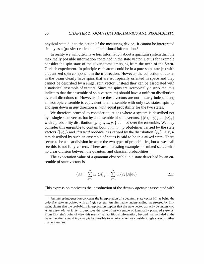
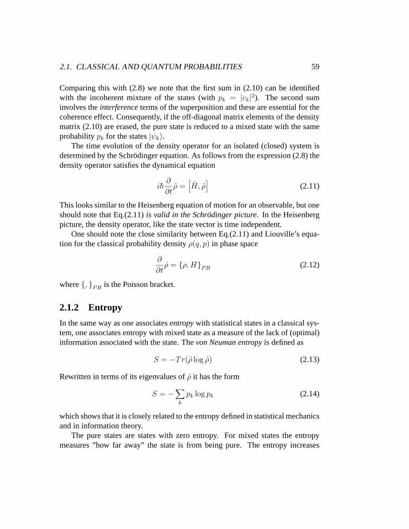
Figure 2.1: The entropy of mixed states for a two level system. The entropy S isshown as a function of the radial variable r for the Bloch sphere representation ofthe states.
states, both pure and mixed can be represented by points in a three dimensionalsphere of radius r = 1. Points on the surface (r = 1) correspond to the purestate. As r decreases the states gets less pure and for r = 0 we find the stateof maximal entropi. The entropi, defined by (2.14), is a monotonic function ofr, with maximum (log 2) for r = 0 and minimum (0) for r = 1. The explicitexpression for the entropi is
S = −(1
2(1 + r) log
1
2(1 + r) +
1
2(1 − r) log
1
2(1 − r)) (2.24)
The sphere of states for the two-level system is called the Bloch sphere. Moregenerally the set of density matrices of a quantum system can be shown to form aconvex set (see Problem (2.4.3)).
2.2 Entanglement
In this section we consider composite systems, which can be considered as con-sisting of two or more subsystems. These subsystems will in general be correlateddue to interactions between the two parts. A quantum system may have correla-tions that in some sense are stronger than what is possible in a classical system.We refer to this effect as quantum entanglement. This is considered as one of theclearest marks of the difference between classical and quantum physics.
2.2. ENTANGLEMENT 63
2.2.1 Composite systems
To this point we have mainly considered an isolated quantum system. Only thevariables of the system then enters in the quantum description, in the form of ofstate vectors and observables, while the dynamical variables of other systems areirrelevant. As long as the system stays isolated all interactions with other systemsare negligible and the time evolution is described by the Schrodinger equation.
With maximal information about the system we describe it by a pure state (astate vector), with less than maximal information it is described by a mixed state(a density matrix). If the system is in a pure state, it will continue to be in a purestate as long as it stays isolated. For a mixed state, the degree of ”non-purity”measured by the entropy will stay constant as long as it is isolated. This followsfrom the fact that the time evolution is unitary and the eigenvalues of the densityoperator therefore do not change with time.
Clearly an isolated system is an abstraction since interactions with other sys-tems (generally referred to as the environment) can never be totally absent. How-ever, in some cases this idealization works perfectly well to a high dergee of acu-racy. If interactions with the environments cannot be neglected, also variablesassociated with the environment have to be taken into account. If these act ran-domly on the system they tend to introduce decoherence in the system. The statedevelops in the direction of being less pure, i.e., the entropy increases. However,a systematic manipulation with the system may change the state in the directionof being more pure. Thus, a partial or full measurement performed on the systemwill be of this kind.
Even if a system A cannot be considered as isolated, sometimes it will be apart of a larger isolated system. We will consider this sitation and assume thatthe total system can be descibed in terms of a set of variables for system A anda set of variables for the rest of the system, which we denote B. We assume thatthese two sets of variables can be regarded as independent (they are associatedwith independent degrees of freedom for the two subsystems A and B), and thatthe interactions between A and B do not destroy this relative independence. Wefurther assume that the totality of dynamical variables for A and B provides acomplete set of variables for the full system. We refer to this as a compositesystem.
The interactions between the two parts of a composite system will introducecorrelations between the two parts. Thus, the evolution of the two subsystems willbe correlated and the expectation values of variables from system A and B will ingeneral also be correlated. Correlations is a typical feature of interacting systems
64 CHAPTER 2. QUANTUM MECHANICS AND PROBABILITY
both at the classical and quantum level. We shall focus here on correlations thatare special for a quantum mechanical system.
In mathematical terms we describe the Hilbert space H of a composite systemas a tensor product of two Hilbert spaces HA and HB associated with the twosubsytems,
H = HA ⊗HB (2.25)
A basis |i〉 of HA and a basis |α〉 of HB then defines a tensor product basis for H,
|iα〉 = |i〉 ⊗ |α〉 (2.26)
A general vector in H is of the form
|χ〉 =∑
iα
ciα|i〉 ⊗ |α〉 (2.27)
and in general it is not a tensor product of a vector from HA with a vector fromHB.
The observables of system A and the observables of system B define commut-ing observables of the full system. This follows directly from how they act on thebasis vectors (2.26). With A as an observable for system A and B as an observablefor system B, we have
A|iα〉 =∑
j
Aji|jα〉 , B|iα〉 =∑
β
Bβα|iβ〉 (2.28)
Clearly
AB|iα〉 =∑
jβ
AjiBβα|jβ〉 = BA|iα〉 (2.29)
The expectation values of observables acting only on subsystem A are deter-mined by the reduced density matrix of system A. This is obtained by taking thepartial trace with respect to the coordinates of system B,
ρA = TrB(ρ) , ρAij =
∑
α
ρiα jα (2.30)
In the same way we define the reduced density matrix for system B
ρB = TrA(ρ) , ρBαβ =
∑
i
ρiα iβ (2.31)
2.2. ENTANGLEMENT 65
In general the reduced density matrices will correspond to mixed states for thesubsystems A and B, even if the full system is in a pure state.
For a composite system there exist certain relations between the entropy S(ρ)of the full system and the entropies of the subsystems, S(ρA) and S(ρB). Thus,for a bipartite system (a system consisting of two parts), like the one consideredabove, the following inequalities are satisfied,
S(ρ) ≤ SA + SB , S(ρ) ≥ |SA − SB| (2.32)
We note in particular the first inequality. This may seem somewhat surprising,since it indicates that there are states of a composite system that are more purethan the states of its subsystems. A corresponding situation for a classical systemwould be rather paradoxical since it would mean that the total system could be ina state that was more ordered than the states of its subsystems. Another way tointerprete the inequality is that full information about the states of the subsystemsA and B will in general not be sufficient to give full information about the state ofthe total system A+B. When there are correlations between the two subsystems,these are not seen in the description of A and B separately.
2.2.2 Correlations and entanglement
A product state of the form
ρ = ρA ⊗ ρB (2.33)
is a state with no correlations between the subsystems A and B. For any observ-able A acting on A and B acting on B the expectation value of the product operatorAB, is then simply the product of the expectation values
〈AB〉 = 〈A〉A 〈B〉B (2.34)
Written in terms of the density operators,
Tr(ρAB) = TrA(ρAA)TrB(ρBB) . (2.35)
Conversely, if the product relation (2.34) is correct for all observables A acting onA and all observables B acting on B, the two subsystems are uncorrelated and thedensity operator can be written in the product form (2.34).
We next consider a (mixed) state of the form
ρ =∑
k
pk ρAk ⊗ ρB
k . (2.36)
66 CHAPTER 2. QUANTUM MECHANICS AND PROBABILITY
With {pk} as a probability distribution, this density matrix can be viewed as de-scribing a statistical ensemble of product states, i.e., of states which, when re-garded separately, do not contain correlations between the two subsytems. How-ever, the density matrix of the ensemble does contain (statistical) correlations be-tween the two subsystems. Thus, the expectation value of a product of observablesfor A and B is
〈AB〉 =∑
k
pk 〈A〉k A 〈B〉k B
=∑
k
pkTrA(ρAk A)TrB(ρB
k B) (2.37)
and this is generally different from the product of expectation values,
〈A〉A 〈B〉B =∑
k
pk 〈A〉k A
∑
l
pl 〈B〉l B
=∑
k l
pk pl TrA(ρAk A)TrB(ρB
l B) . (2.38)
The correlations contained in a density operator of the form (2.36) we mayrefer to as classical correlations, since these are of the same form that we find ina classical, statistical description of a composite system. However, in a quantumsystem there may be correlations that cannot be written in the form (2.36) andwhich are therefore of genuinely quantum mechanical nature. Composite sys-tems with this kind of correlations are said to be entangled, and in some sense thecorrelations that are found in entangled states are stronger than can be achieveddue to classical statistical correlations. In recent years there has been much effortdevoted to give a concise quantiative meaning to entanglement in composite sys-tems. However, for bipartite systems in mixed states and for multipartite systemsin general, it is not obvious how to quantify deviations from classical correla-tions. But for a bipartite system in a pure state the definition of entanglement isunambiguous. We focus on this case.
We therfore now consider a general pure state of the total system A+B. Theentropy of such a state clearly vanishes. The state has the general form
|χ〉 =∑
iα
ciα|i〉A ⊗ |α〉B (2.39)
but can also be written in the diagonal form
|χ〉 =∑
n
dn|n〉A ⊗ |n〉B (2.40)
2.2. ENTANGLEMENT 67
where {|n〉A} is a set of orthonormal states for the A system and {|n〉B} is a setof orthonormal states for the B system. This form of the state vector as a simplesum over product vectors rather than a double sum is referred to as the Schmidtdecomposition of |χ〉. It can be shown to be generally valid for a composite two-partite system.
The form of the state vector |χ〉 is similar to that of density operator (2.36)for the correlated state. In the same way as for the density operator the system isuncorrelated if the sum includes only one term, i.e., if the state has a product form.However, the correlations implied by the general form of the state vector (2.40) aredifferent from those of the (classically) correlated state (2.36). From the Schmidtdecomposition follows that the density matrix of the full system corresponding tothe pure state |χ〉 is
ρ =∑
nm
dnd∗m |n〉A〈m|A ⊗ |n〉B〈m|B (2.41)
This is not of the form (2.36). The state (2.40) has correlations between statevectors of the two subsystems rather than correlations only between density oper-ators.
From (2.41) also follows that the reduced density operators of the two subsys-tems have the form
ρA =∑
n
|dn|2|n〉A〈n|A , ρB =∑
n
|dn|2|n〉B〈n|B (2.42)
The expressions show that all the eigenvalues of the two reduced density matricesare the same. This implies that the von Neuman entropy of the two subsystems isthe same,
SA = SB = −∑
n
|dn|2 log |dn|2 (2.43)
In this case, with the full system A+B in a pure state, the entropy of one of thesubsystems (A or B) is taken as a quantitative measure of the entanglement be-tween the subsystems.
The Schmidt decompositionWe show here that a general state of the composite system can be written in theform (2.40). The starting point is the general expression (2.39). We introduce aunitary transformation U for the basis of system A,
|i〉A =∑
m
Umi |m〉A (2.44)
68 CHAPTER 2. QUANTUM MECHANICS AND PROBABILITY
and rewrite the state vector as
|χ〉 =∑
iα
∑
m
ciαUmi|m〉A ⊗ |α〉B
=∑
m
|m〉A ⊗ (∑
iα
ciαUmi|α〉B)
≡∑
m
|m〉A ⊗ |m〉B (2.45)
If the unitary transformation can be chosen to make the set of states {|m〉} andorthogonal set of states, then (2.40) follows. The scalar product between two ofthe states is
〈n|m〉B =∑
iα
∑
jβ
c∗jβU∗njciαUmi〈β|α〉B
=∑
ij
∑
α
c∗jαU∗njciαUmi
= (UCC†U †)mn (2.46)
In the last expression the coefficients ciα have been treated as the matrix elementsof the matrix C. We note that the matrix M = CC† is a hermitian, positivedefinite operator and the unitary matrix U can therefore be chosen to diagonalizeM . With the (non-negative) eigenvalues written as |dn|2 we have
〈n|m〉B = |dn|2δmn (2.47)
and if the normalized vectors |m〉 are introduced by
|m〉 = dm|m〉 (2.48)
then the Schmidt form (2.40) of the vector |χ〉 is reproduced with the basis sets ofboth systems A and B as orthonormal vectors.
2.2.3 Entanglement in a two-spin system
To exemplify this we consider the simplest possible composite system, a systemthat consists of two two-level subsystems (for example two spin-half systems).We shall consider several sets of vectors with different degrees of entanglement.
2.2. ENTANGLEMENT 69
An orthogonal basis of product states is given by the four vectors
| ↑ ↑〉 = | ↑〉A ⊗ | ↑〉B| ↑ ↓〉 = | ↑〉A ⊗ | ↓〉B| ↓ ↑〉 = | ↓〉A ⊗ | ↑〉B| ↓ ↓〉 = | ↓〉A ⊗ | ↓〉B (2.49)
where {| ↑〉, | ↓〉} is an orthonormal basis set for the spin-half system.Another basis is given by those with well-defined total spin. As is well-known
by the rules of addition of angular momentum, two spin half systems will havestates of total spin 0 or 1. The spin 0 state is the antisymmetric (spin singlet) state
|0〉 =1√2(| ↑ ↓〉 − | ↓ ↑〉) (2.50)
while spin 1 is described by the symmetric (spin triplet) states
|1, ↑〉 = | ↑ ↑〉 , |1, 0〉 =1√2(| ↑ ↓〉 + | ↓ ↑〉) , |1, ↓〉 = | ↓ ↓〉 (2.51)
Clearly the two states |1, ↑〉 = | ↑ ↑〉 and |1, ↓〉 = | ↓ ↓〉 are product states withno correlation between the two spin systems. However, the two remaining states|0〉 and |1, 0〉 are entangled. These states may be included as two of the states of athird basis of orthonormal states, called the Bell states. They are defined by
|a,±〉 =1√2(| ↑ ↓〉 ± | ↓ ↑〉)
|c,±〉 =1√2(| ↑ ↑〉 ± | ↓ ↓〉) (2.52)
and are all states of maximal entanglement between the two subsystems. We notethat the two spins are strictly anticorrelated for the first two states (|a,±〉) andstrictly correlated for the two other states (|c,±〉).
Let us focus on the spin singlet state |a,−〉. It is a pure state (of system A+B)with density matrix
ρ(a,−) = |a,−〉〈a,−|
=1
2(| ↑ ↓〉〈↑ ↓ | + | ↓ ↑〉〈↓ ↑ | − | ↑ ↓〉〈↓ ↑ | − | ↓ ↑〉〈↑ ↓ |)
(2.53)
70 CHAPTER 2. QUANTUM MECHANICS AND PROBABILITY
The corresponding reduced density matrices of both systems A and B are of thesame form
ρA = ρB =1
2(| ↑〉〈↑ | + | ↓〉〈↓ |) (2.54)
The symmetric state ρ(a, +) has the same reduced density matrices as ρ(a,−). Infact this is true for all the four Bell states. Thus, the information contained in thedensity matrices of the subsystems do not distinguish between these four states ofthe total system.
The loss of information when we consider the reduced density matrices isdemonstrated explicitly in taking the partial trace of (2.53) with respect to sub-system A or subsystem B. The two last terms in (2.53) simply do not contribute.If we leave out the two last terms of (2.53) we have the following density matrix,which also have the same reduced density matrices,
ρ(a) =1
2(| ↑ ↓〉〈↑ ↓ | + | ↓ ↑〉〈↓ ↑ |) (2.55)
This is still strictly anticorrelated in the spin of the two particles, but the correla-tion is now classical in the sense that the full density matrix is written in the form(2.36). Thus, the terms that are important for the quantum entanglement betweenthe two subsystems are the ones that are left out when we take the partial trace.These terms are the off-diagonal interference terms of the full density matrix, andthis means that we can view the entanglement as a special type of interferenceeffect associated with the composite system.
When the reduced density operators are written as 2 × 2 matrices they havethe form
ρA = ρB =1
2
(1 00 1
)(2.56)
Thus they are proportional to the 2 × 2 unit operator and therefore correspond tostates with maximal entropy SA = SB = log 2. With the entropy of the subsys-tems taken as a measure of entanglement this means that the spin singlet state is astate of maximal entanglement. This is true for all the Bell states, as already hasbeen mentioned.
Finally, note that the reduced density matrices (3.8) are rotationally invariant.This is however not the case for the “classical” density matrix (2.55) of the fullsystem. It describes a state where the spins of the two particles along one particu-lar direction is strictly anticorrelated. It is interesting to note that we cannot definea density matrix of this form which predicts strict anticorrelation for the spin in
2.3. QUANTUM STATES AND PHYSICAL REALITY 71
any direction. Also note that neither the pure state |a, +〉 is rotationally invariant.In fact the state |a,−〉 is the only Bell state that is rotationally inavriant, since itcorresponds to spin 0. This makes the spin singlet state particularly interesting,since it describes a situation where the spins are strictly anticorrelated along anydirection in space.
2.3 Quantum states and physical reality
In 1935 Einstein, Podolsky and Rosen published a paper where they focussed on acentral question in quantum mechanics. This question has to do with the relationbetween the the formalism of quantum mechanics, with its probability interpreta-tion, and the underlying physical reality that quantum mechanics describes. Theypointed out, by way of a simple thought experiment, that one of the implicationsof quantum physics is that it blurs the distinction between the objective reality ofnature and the subjective description used by the physicist. Their thought exper-iment has been referred to as the EPR paradox, and it has challenged physicistsin their understanding of the relation between physics and the reality of naturalphenomena up to this day. Einstein strongly suggested that the paradox showedthat quantum mechanics is an incomplete theory of nature. Later, in 1964 JohnBell showed that the conflict between quantum mechanics and intuitive notions ofreality goes deeper. Quantum theory allows types of correlations that cannot befound in classical theories that obey the basic assumptions of locality and reality.
In this section we examine the EPR paradox in a form introduced by DavidBohm and proceed to examine how the limitations of classical theory is broken inthe form of Bell inequalities. As first emphasized by Erwin Schrodinger the basicelement of quantum physics involved in these considerations is that of entangle-ment.
2.3.1 EPR-paradox
We consider a thought experiment, where two spin half particles (particle A andparticle B) are produced in a singlet state (with total spin zero). The two particlesmove apart, but since they are considered to be well separated from any distur-bance, they keep their correlation so that the spin state is left unchanged. Thefull wave function of the two-particle system can be viewed as the product of aspin state and a position state, but for our purpose only the spin state is of inter-est. Concerning the position state it is sufficient to know that after some time the
72 CHAPTER 2. QUANTUM MECHANICS AND PROBABILITY
particles are separated by a large distance.At a point in time when the two particles are well separated, a spin measure-
ment is performed on particle A. This will modify the spin state of this particle,but since particle B is far away, the measurement cannot affect particle B in anyreal sense. However, and this is the paradox, the change in the spin state caused bythe measurement will also influence the possible outcomes of spin measurementsperformed on particle B.
The experiment is outlined in Fig.(2.3.1). From the time when the particles areemitted and until the time when the spin experiment is performed the two particlesare in the entangled state
|a,−〉 =1√2(| ↑ ↓〉 − | ↓ ↑〉) (2.57)
In this state the spin of the two particles are strictly anticorrelated. This meansthat if particle A is measured to be in a spin up state, particle B is necessarilyin a spin down state. But each particle, when viewed separately, is with equalprobability found with spin up and spin down.
The reference to spin up (↑) and spin down (↓) in the state vector (2.57) seemsto indicate that we have given preference to some particular direction in space.However, the singlet state is rotationally invariant. Therefor the state is left un-changed if we redefine this direction in space. Thus, we do not have to specifywhether the z-axis, the x-axis or any other direction has been chosen, they all giverise to the same (spin 0) state.
We now consider, in this hypothetical experiment, that the spin of particle ismeasured along the z-axis. If the result is spin up, we know with certainty thatthe spin of particle B in the z-direction is spin down. Likewise, if the result ofmeasurement on A is spin down the spin of particle B in the z-direction is spinup. In both cases, a measurement of the z spin component of particle A will withnecessity project particle B into a state with well defined (quantized) z-componentof the spin. Since no real change can have been introduced in the state of particleB (it is far away) it seems natural to conclude that the spin component along the z-axis must have had a sharp (although unknown value) also before the measurementwas actually performed on particle A.
This conclusion is on the other hand in conflict with the standard interpre-tation of quantum mechanics. If the the z-component of the spin of particle Ahas a sharp value before the measurement, it will have a sharp value even if themeasurement along the z-axis is not performed at all, and even if we choose to
2.3. QUANTUM STATES AND PHYSICAL REALITY 73
S
AB
MAMB
entangled
S
AB
MAMB
( a )
( b )
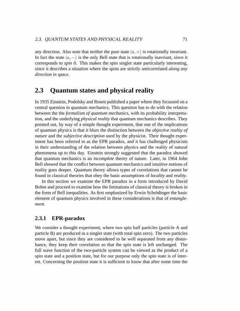
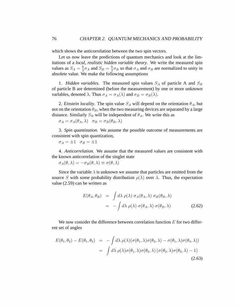
Figure 2.2: The set-up of an EPR experiment. Two entangled particles in a singletspin state is sendt in opposite directions from a source S. The particles are shownat three different times. The spin direction of each particle is, in this initial state,totally undetermined. In Fig (a) the z-component of the spin of particle A ismeasured by a measuring device MA at a time tMA
. Since the spins of the twoparticles are strictly anticorrelated this measurement will project not only particleA, but also particle B into a state of quantized spin in the z-direction. If oneassumes (like EPR) that no real change has taken place at the position of particleB, one may be tempted to conclude that particle B was in reality in this spinstate also before the measurent. In Fig (b) the measurement by MA is changedto a rotated direction. Repeating the argument would lead to the conclusion thatparticle B had a well-defined (although unknown) spin component in this directionbefore the measurement. But before the measurement one has a freedom of choicein what direction to perform the measurement, either in the direction of (a) or thedirection of (b). This seems to indicate that both spin components have to bewell defined before the measurement. But the two components of the spin areincompatible observables, hence the paradox.
74 CHAPTER 2. QUANTUM MECHANICS AND PROBABILITY
measure the spin along the x-axis instead. But now the argument can be repeatedfor the x-component of the spin. This will in the same way lead to the conclu-sion that the x-component of the spin of particle has a sharp value before themeasurement. Consequently, both the z-component and the x-component of thespin must have a sharp value before the measurement is performed on particle A.But this is not in accordance with the standard interpretation of quantum mechan-ics. The z-component and the x-component of the spin operator are incompatibleobservables, since they do not commute as operators. Therefore they cannot si-multanuously be assigned sharp values.
The conclusion Einstein, Podolsky and Rosen drew from the thought experi-ment is that both observables will in reality have sharp values, but since quantummechanics is not able to predict these values with certainty (only with probabili-ties) quantum theory cannot be a complete theory of nature. From their point ofview there seem to be some missing variables in the theory. If such variables areintroduced, we refer to the theory as a “hidden variable” theory.
Note the two elements that enter into the above argument:Locality — Since particle B is far away from where the measurement takes placewe conclude that no real change can take place concerning the state of particle B.Reality — When the measurement on particle A makes it possible to predict withcertainty the outcome of a measurement performed on particle B, we draw theconclusion that this represents a property of B which is there even without actuallyperforming a measurement on B.
From later studies we know that the idea of Einstein, Podolsky and Rosen thatquantum theory is an incomplete theory does not really resolve the EPR paradox.Hidden variable theories can in principle be introduced, but to be consistent withthe predictions of quantum mechanics, they cannot satisfy the conditions of lo-cality and reality used by EPR. Thus, there is a real conflict between quantummechanics and basic principles of classical theories of nature.
From the discussion above it is clear that entanglement between the two par-ticles is the source of the (apparent) problem. It seams natural to draw the con-clusion that if a measurement is performed on one of the partners of an entangledsystem there will be (immediately) a change in the state also of the other partner.But if we phrase the effect in this way, one should be aware of the fact that theeffect of entanglement is always hidden in correlations between measurementsperformed on the two parts. The measurement performed on particle A does notlead to any local change at particle B that can be seen without consulting the re-sult of the measurement performed on A. Thus, no change that can be interpretedas a signal sent from A to B has taken place. This means that the immediate
2.3. QUANTUM STATES AND PHYSICAL REALITY 75
change that is affecting the total system A+B due to the measurement on A doesnot introduce results that are in conflict with causality.
2.3.2 Bell’s inequality
Correlation functionsThe EPR paradox shows that quantum mechanics is radically different from clas-sical statistical theories when entanglement between systems is involved. In theoriginal presentation of Einstein, Podolsky and Rosen it was left open as a possi-bility that a more complete description of nature could replace quantum mechan-ics. However, by studying correlations between spin systems John Bell concludedin 1964 that the predictions of quantum mechanics is in direct conflict with whatcan be deduced from a “more complete” theory with hidden variables, when thissatisfy what is known as Einstein locality. This was expressed in terms of a cer-tain inequality (Bell inequality) that has to be satisfied by classical (local, realistic)theories. Quantum theory does not satisfy this inequality.
To examine this difference between classical and quantum correlations wereconsider the EPR experiment, but focus on correlations between measurementsof spin components performed on both particles A and B. Let us assume that theparticles move in the x-direction. The spin component in a rotated direction in they, z-plane will have the form
Sθ = cos θSz + sin θSx (2.58)
We consider now the following correlation function between spin measurementson the two particles,
E(θA, θB) ≡ 4
h2 〈SθASθB
〉 (2.59)
Thus, we are interested in correlations between spin directions that are rotatedby arbitrary angles θA and θB in the y, z-plane. The factor h2/4 is included tomake E(θA, θB) a dimensionless function, normalized to take values in the inter-val (−1, +1).
For the spin singlet state it is easy to calculate this correlation function. It is
E(θA, θB) = − cos(θA − θB) (2.60)
With the two spin measurements oriented in the same direction, θA = θB ≡ θ, wehave
E(θ, θ) = −1 (2.61)
76 CHAPTER 2. QUANTUM MECHANICS AND PROBABILITY
which shows the anticorrelation between the two spin vectors.Let us now leave the predictions of quantum mechanics and look at the lim-
itations of a local, realistic hidden variable theory. We write the measured spinvalues as SA = h
2σA and SB = h
2σB so that σA and σB are normalized to unity in
absolete value. We make the following assumptions
1. Hidden variables. The measured spin values SA of particle A and SB
of particle B are determined (before the measurement) by one or more unknownvarlables, denoted λ. Thus σA = σA(λ) and σB = σB(λ).
2. Einstein locality. The spin value SA will depend on the orientation θA, butnot on the orientation θB, when the two measuring devices are separated by a largedistance. Similarly SB will be independent of θA. We write this as
σA = σA(θA, λ) σB = σB(θB, λ)
3. Spin quantization. We assume the possible outcome of measurements areconsistent with spin quantization,
σA = ±1 σB = ±1
4. Anticorrelation. We assume that the measured values are consistent withthe known anticorrelation of the singlet state
σA(θ, λ) = −σB(θ, λ) ≡ σ(θ, λ)
Since the variable λ is unknown we assume that particles are emitted from thesource S with some probability distribution ρ(λ) over λ. Thus, the expectationvalue (2.59) can be written as
E(θA, θB) =∫
dλ ρ(λ) σA(θA, λ) σB(θB, λ)
= −∫
dλ ρ(λ) σ(θA, λ) σ(θB, λ) (2.62)
We now consider the difference between correlation function E for two differ-ent set of angles
E(θ1, θ2) − E(θ1, θ3) = −∫
dλ ρ(λ)(σ(θ1, λ)σ(θ2, λ) − σ(θ1, λ)σ(θ3, λ))
=∫
dλ ρ(λ)σ(θ1, λ)σ(θ2, λ) (σ(θ2, λ)σ(θ3, λ) − 1)
(2.63)
2.3. QUANTUM STATES AND PHYSICAL REALITY 77
In the last expression we have used σ(θ, λ)2 = 1, which follows from assumption3. From this we deduce the following inequality
|E(θ1, θ2) − E(θ1, θ3)| ≤∫
dλ ρ(λ) (1 − σ(θ2, λ)σ(θ3, λ))
= 1 + E(θ2, θ3) (2.64)
which is one of the forms of the Bell inequality.Let us make the further assumption that the correlation function is only depen-
dent on the relative angle (rotational invariance),
E(θ1, θ2) = E(θ1 − θ2) (2.65)
Let us also assume that E(θ) increases monotonically with θ in the interval (0, π).(Both these assumptions are true for the quantum mechanical correlation function(2.60).) We introduce the probability function
P (θ) =1
2(E(θ) + 1) (2.66)
This function gives the probability for measuring either spin up or spin downon both spin measurements (see the discussion below). It satisfies the simplifiedinequality
P (2θ) ≤ 2P (θ) , 0 ≤ θ ≤ π
2(2.67)
Due to strict anticorrelation between the spin measurements for θ = 0, whichmeans strict correlation for θ = π, the function satisfies the boundary conditions
P (0) = 0 , P (π) = 1 (2.68)
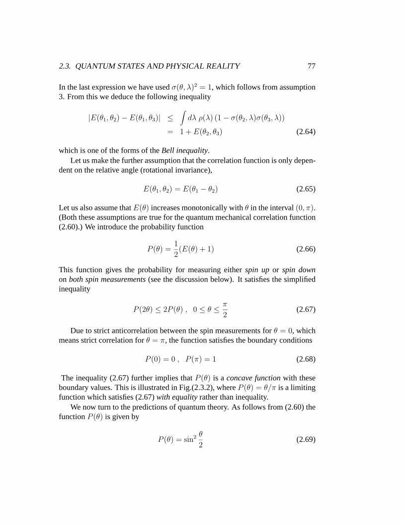
The inequality (2.67) further implies that P (θ) is a concave function with theseboundary values. This is illustrated in Fig.(2.3.2), where P (θ) = θ/π is a limitingfunction which satisfies (2.67) with equality rather than inequality.
We now turn to the predictions of quantum theory. As follows from (2.60) thefunction P (θ) is given by
P (θ) = sin2 θ
2(2.69)
78 CHAPTER 2. QUANTUM MECHANICS AND PROBABILITY
0.5 1 1.5 2 2.5 3
0.2
0.4
0.6
0.8
1 P(Θ)
Θ
A
B
C
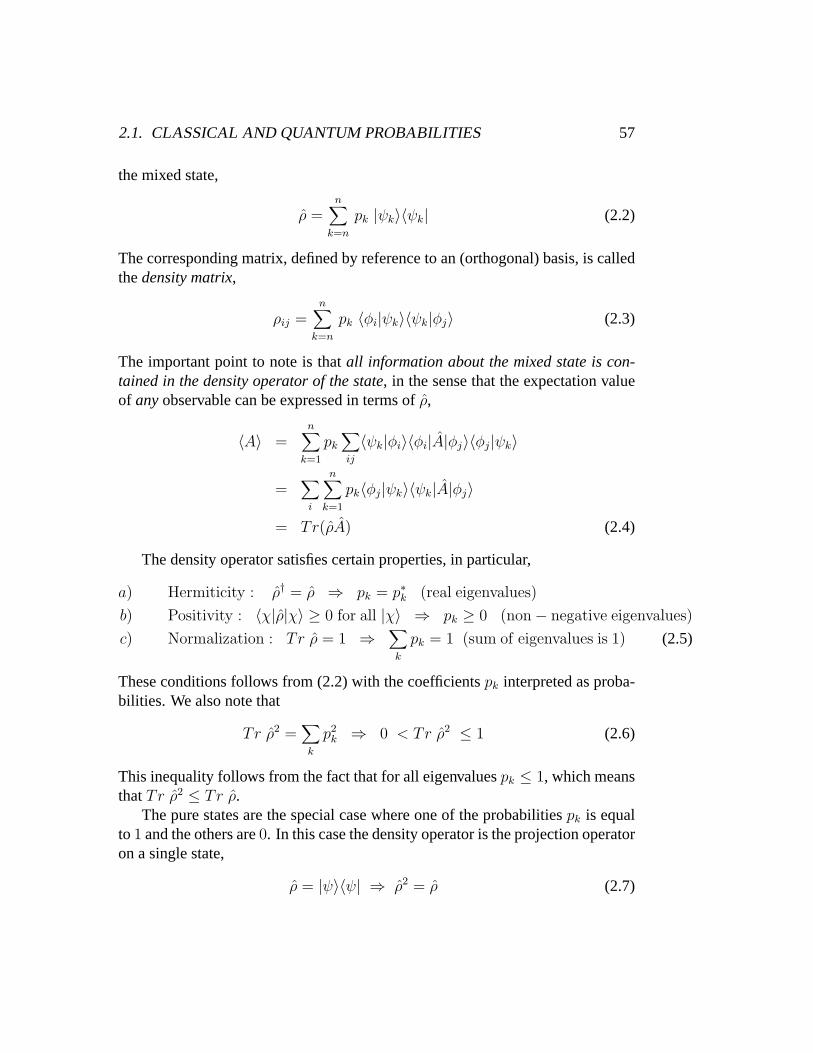
Figure 2.3: The probability P (θ) for measuring two spin ups or two spin downsas a function of the relative angle θ between the spin directions. Curve A sat-isfies the Bell inequality, Curve B is the limiting case where the Bell inequalityis replaced by equality and Curve C is the probability predicted by quantum me-chanics. Curve C is not consistent with the Bell inequality, but is confirmed byexperiment.
This function does not satisfy the Bell inequality. This is clear from taking aspecial value θ = π/3. We have
P (2π/3) = sin2 π
3=
3
4
2P (π/3) = 2 sin2 π
6=
1
2(2.70)
Thus, P (2π/3) > 2P (π/3) in clear contradiction to Bell’s inequality. This break-ing of the inequality is seen also in Fig.(2.3.2).
Measured frequenciesTo get a better understanding of the physical content of the Bell inequality wewill discuss its meaning in the context of spin measurements performed on thetwo particles, where a series of results spin up or spin down is registered for eachparticle. We are particularly interested in correlations between the results of pairsof entangled particles.
Let us therefore consider a spin measurement experiment where the orienta-tions of the two measurement devices are set to fixed directions. We assume Npairs of entangled particles are used for the experiment. The results are registered
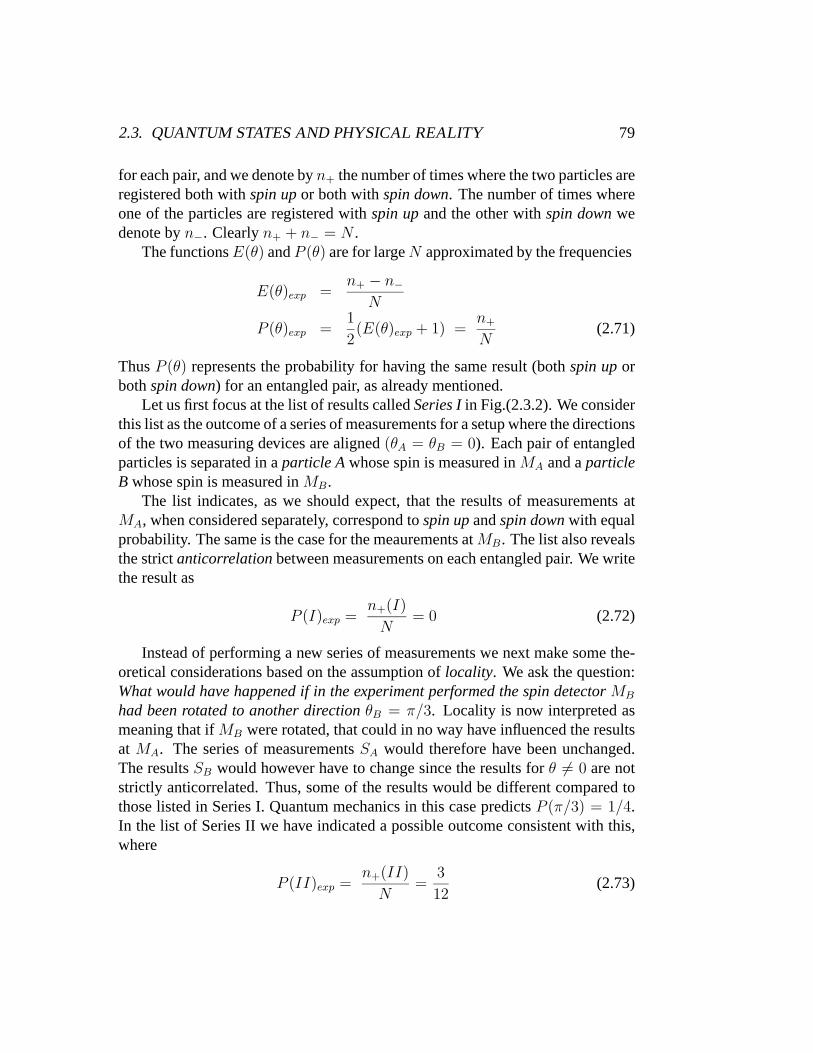
2.3. QUANTUM STATES AND PHYSICAL REALITY 79
for each pair, and we denote by n+ the number of times where the two particles areregistered both with spin up or both with spin down. The number of times whereone of the particles are registered with spin up and the other with spin down wedenote by n−. Clearly n+ + n− = N .
The functions E(θ) and P (θ) are for large N approximated by the frequencies
E(θ)exp =n+ − n−
N
P (θ)exp =1
2(E(θ)exp + 1) =
n+
N(2.71)
Thus P (θ) represents the probability for having the same result (both spin up orboth spin down) for an entangled pair, as already mentioned.
Let us first focus at the list of results called Series I in Fig.(2.3.2). We considerthis list as the outcome of a series of measurements for a setup where the directionsof the two measuring devices are aligned (θA = θB = 0). Each pair of entangledparticles is separated in a particle A whose spin is measured in MA and a particleB whose spin is measured in MB.
The list indicates, as we should expect, that the results of measurements atMA, when considered separately, correspond to spin up and spin down with equalprobability. The same is the case for the meaurements at MB. The list also revealsthe strict anticorrelation between measurements on each entangled pair. We writethe result as
P (I)exp =n+(I)
N= 0 (2.72)
Instead of performing a new series of measurements we next make some the-oretical considerations based on the assumption of locality. We ask the question:What would have happened if in the experiment performed the spin detector MB
had been rotated to another direction θB = π/3. Locality is now interpreted asmeaning that if MB were rotated, that could in no way have influenced the resultsat MA. The series of measurements SA would therefore have been unchanged.The results SB would however have to change since the results for θ �= 0 are notstrictly anticorrelated. Thus, some of the results would be different compared tothose listed in Series I. Quantum mechanics in this case predicts P (π/3) = 1/4.In the list of Series II we have indicated a possible outcome consistent with this,where
P (II)exp =n+(II)
N=
3
12(2.73)
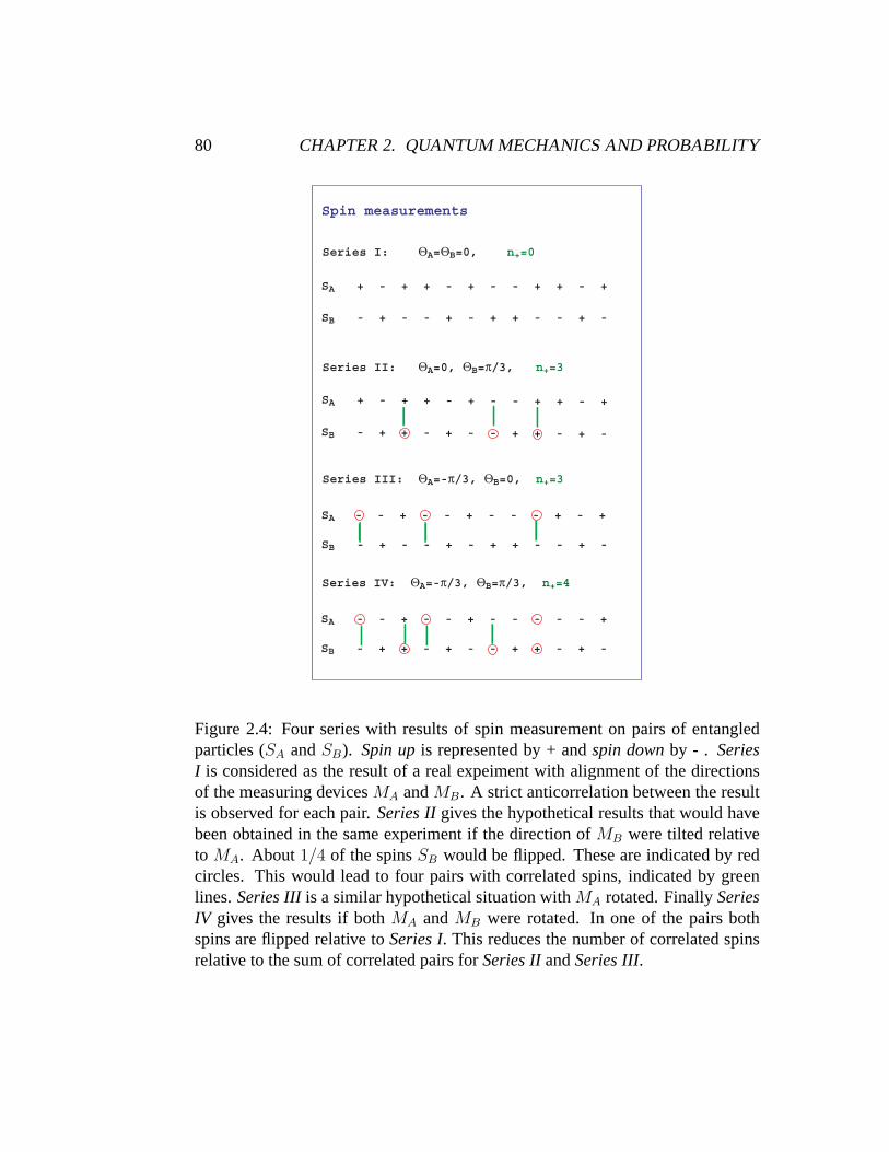
80 CHAPTER 2. QUANTUM MECHANICS AND PROBABILITY
SA + - + + - + - - + + - +
SB - + - - + - + + - - + -
Series I: ΘA=ΘB=0, n+=0
Spin measurements
SA + - + + - + - - + + - +
SB - + + - + - - + + - + -
Series II: ΘA=0, ΘB=π/3, n+=3
SA - - + - - + - - - + - +
SB - + - - + - + + - - + -
Series III: ΘA=-π/3, ΘB=0, n+=3
SA - - + - - + - - - - - +
SB - + + - + - - + + - + -
Series IV: ΘA=-π/3, ΘB=π/3, n+=4
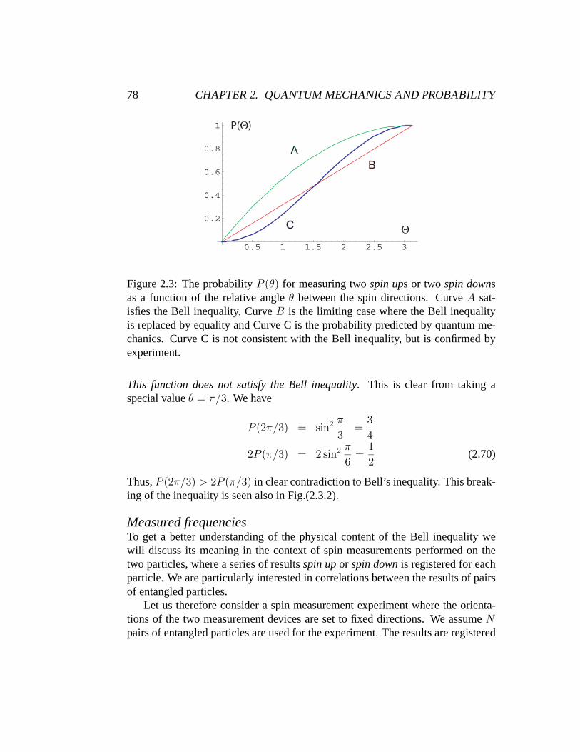
Figure 2.4: Four series with results of spin measurement on pairs of entangledparticles (SA and SB). Spin up is represented by + and spin down by - . SeriesI is considered as the result of a real expeiment with alignment of the directionsof the measuring devices MA and MB. A strict anticorrelation between the resultis observed for each pair. Series II gives the hypothetical results that would havebeen obtained in the same experiment if the direction of MB were tilted relativeto MA. About 1/4 of the spins SB would be flipped. These are indicated by redcircles. This would lead to four pairs with correlated spins, indicated by greenlines. Series III is a similar hypothetical situation with MA rotated. Finally SeriesIV gives the results if both MA and MB were rotated. In one of the pairs bothspins are flipped relative to Series I. This reduces the number of correlated spinsrelative to the sum of correlated pairs for Series II and Series III.
2.3. QUANTUM STATES AND PHYSICAL REALITY 81
Since we have a symmetric situation between MA and MB we clearly couldhave used the same argument if MA were rotated instead of MB. This situation isshown in Series III, where the series of measurements SB is left unchanged, butsome of the results of SA are changed. In this case we have chosen θA = −π/3.We also in this list have
P (III)exp =n+(III)
N=
3
12(2.74)
consistent with the predictions of quantum mechanics.Finally, we combine these two results to a two-step argument for what would
have happened if both measurement devices had been rotated, to the directionsθA = −π/3 and θB = π/3. We can start with either Series II or Series III.Rotation of the second measuring device would then lead to a change of about1/4 of the results in the series that was not changed in the first step. The totalnumber of correlated pairs would now be
n(IV ) = n(II) + n(III) − ∆ (2.75)
In this expression n(II) is the number of flips in the result of SB and n(III)the number of flips in the results of SA. Such flips would change the result fromanticorrelated to correlated. However that would be true only if only one of thespin results of an entangled pair were flipped. If both spins were flipped we wouldbe back to the situation with anticorrelations. Thus the number of correlated pairswould be equal to the sum of the number of flips in each series minus the numberwhere two flips is applied to the same pair. The last number is represented by ∆in the formula (2.75). In the result of Series IV this is represented by the result
P (IV )exp =n+(IV )
N=
4
12
< P (II)exp + P (III)exp =6
12(2.76)
The subtraction of ∆ in (2.75) explains the Bell inequality, which here takes theform
P (2π/3) ≤ 2P (π/3) (2.77)
The results extracted from the series of spin measurements listed in Fig.(2.3.2)gives (2.76) in accordance with the Bell inequality (2.77).
82 CHAPTER 2. QUANTUM MECHANICS AND PROBABILITY
The arguments given above, which reproduce Bell’s inequality, may seem toimplement the assumption of locality in a very straight forward way: Changesin the set up of the measurements at MA cannot influence the result of measure-ments performed at MB when these devices are separated by a large distance. Thepredictions of quantum mechanics, on the other hand, are not consistent with theresults of these hypothetical experiments, and real experiments have confirmedquantum mechanics rather than the Bell inequality.
So is there anything about the arguments given for the hypothetical experi-ments that indicates that they may be wrong? We note at least one disturbingfact. Only one of the four series of results in Fig.(2.3.2) can be associated with areal experiment. The others must be based on assumptions of what would havehappened if the same series of measururements would have been performed undersomewhat different conditions. This is essential for the result. If the four series ofmeasurements should instead correspond to four different (real) experiments thesituation would be different. We then would have no reason to believe that theseries of results SA would be preserved when going from I to II or SB when goingfrom I to II. Each series would in this case rather give a new (random) distributionof results for particle A (or particle B).
In any case the conclusion seems inevitable, that quantum mechanics is inconflict with Einstein locality, i.e., with the basic assumptions that lead to the Bellinequality. Does this mean that some kind of influence is transmitted from A to Bwhen measuring on particle A, even when the two particles are very far apart?
2.4 Problems
(To be completed.)
2.4.1 Density matrix and spin orientation
a) Write up the general expression for the (2 × 2) density matrix ρ of a spin halfsystem. (It should satisfy the conditions (2.5)). Show that it can be interpretedas representating a statistical ensemble of spin up states and spin down states insome direction n. Find the probabilities p+ for spin up and p− for spin up as wellas the unit vector n expressed in terms of the matrix elements of ρ. Is the vectorn uniquely determined? Discuss the special case where the vector is completelyundetermined.
2.4. PROBLEMS 83
b) Assume the spin-half system is in a pure state. Find the density matrix(or state vector) expressed in terms of the expectation values 〈Sz〉 and 〈Sx〉. (Isinformation about 〈Sy〉 also needed to specify the state?)
c) Assume the spin-half system is in a mixed state. Consider the same questionas under b).
2.4.2 Spin 1 system
Find the number of parameters that determine the general density matrix of a spin1 system. How many parameters are needed if the system is in a pure state?Assume the expectation values 〈Sx〉, 〈Sy〉 and 〈Sz〉 are known. What additionalinformation is needed in the two cases in order to specify the state?
2.4.3 Convexity
Density matrices do not satisfy the superposition principle like the state vectors.They do however satisfy a convexity criteria in the following form. If ρ1 and ρ2 aretwo density matrices, also the following linear combination is a density matrix,
ρ = αρ1 + (1 − α)ρ2 (2.78)
with α as a real number in the interval 0 ≤ α ≤ 1. Show this. Can a pure state bewritten as such a combination of two other density matrices?
2.4.4 Schmidt decomposition
A composite system consists of two two-level systems. The Hilbert space of thecomposite system is spanned by the four vectors
|00〉 = |0〉 ⊗ |0〉 , |01〉 = |0〉 ⊗ |1〉 , |10〉 = |1〉 ⊗ |0〉 , |11〉 = |1〉 ⊗ |1〉 (2.79)
Find the Schmidt decomposition of the following three vectors
|a〉 =1√2(|00〉 + |11〉
|b〉 =1√3(|00〉 + |01〉 + |10〉)
|c〉 =1
2(|00〉 + |01〉 + |10〉 + |11〉)
(2.80)
84 CHAPTER 2. QUANTUM MECHANICS AND PROBABILITY


![Quantum Mechanics relativistic quantum mechanics (RQM) · Quantum Mechanics_ relativistic quantum mechanics (RQM) ... [2] A postulate of quantum mechanics is that the time evolution](https://img.pdfslide.net/doc/110x75/5b6dfe707f8b9aed178e053e/quantum-mechanics-relativistic-quantum-mechanics-rqm-quantum-mechanics-relativistic.jpg)