Chapter 20Chapter 20

Cost Minimization

Basic modelBasic model: :

min x1, x2 w1 x1 + w2 x2 subject to f (x1 , x2 ) = ygives c ( w1 , w2 , y )

Isocost lines: p351

x2 = C/w2 – w1x1/w2.

Tangency of an isocost line and an isoquant.

– MP1 (x1, x2) / MP2 (x1, x2 )= TRS(x1, x2 ) = – w 1 / w 2

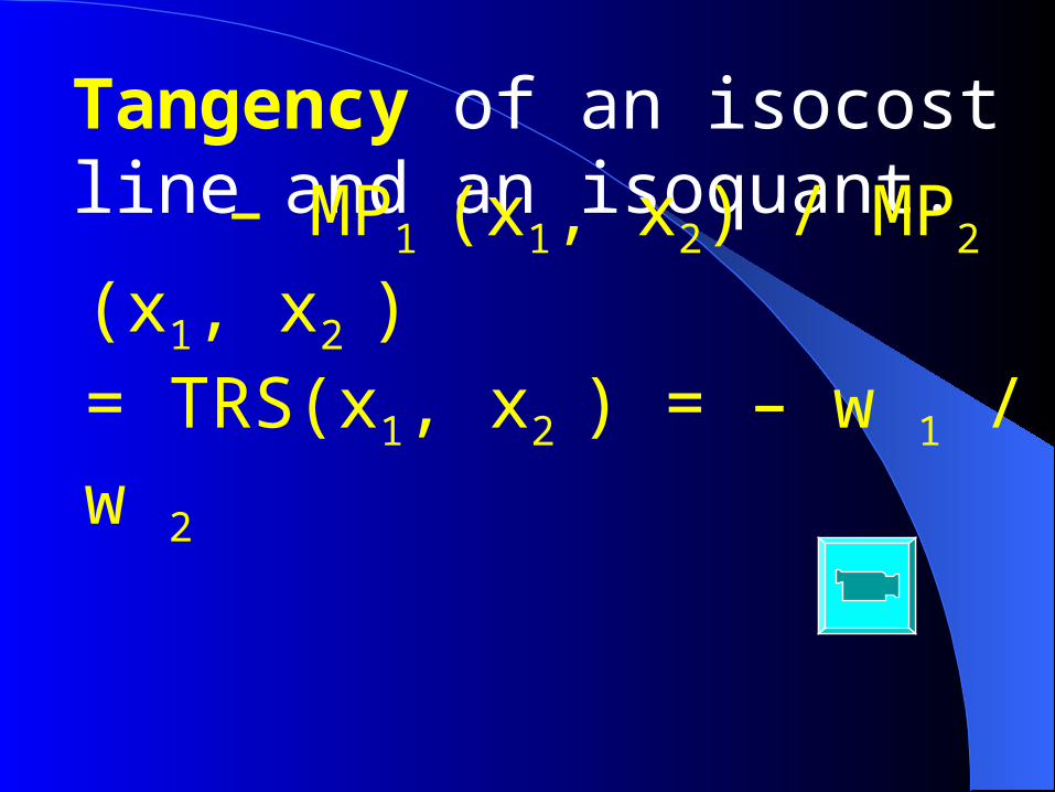
Isocost lines slope= – w 1 / w 2

Isoquant f (x1 , x2 ) = y

Optimal choice

x2*

x2

x1* x1

.

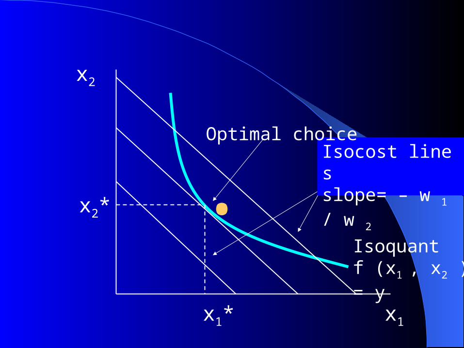
Minimizing costs for

y = min{ax1 , bx2}; 完全互补 y = ax1 + bx2; 完全替代 and y = x1

a x2b. Cobb-Dougl

as

Fixed and variable costs.

(FC and VC)

Total, average, marginal, and average variable costs. (TC, AC, MC and AVC)

MC > (<) AC if and only if AC is increasing (decreasing)

MC cuts AC (AVC) at AC’s (AVC’s) extreme.

MC

AVC

AC

y

ACAVCMC

..

Chapter 21Chapter 21

Cost

Curves

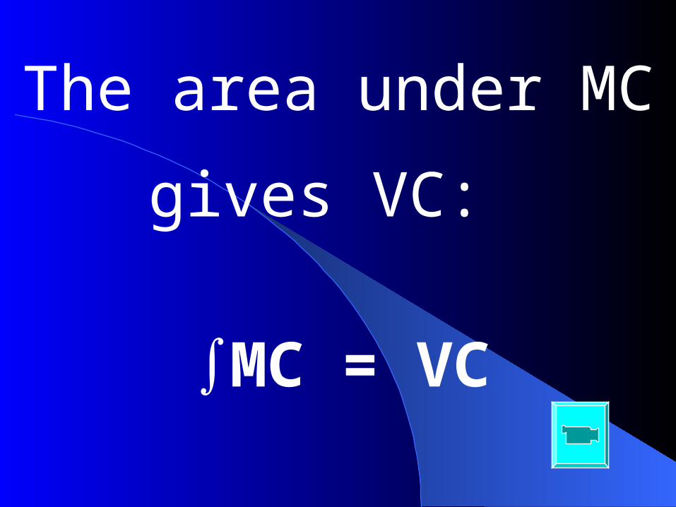
The area under MC

gives VC:

∫MC = VC

MC

Variable costs

MC

y

Division of output Division of output among plants of a firm.among plants of a firm.

MC1

MC2

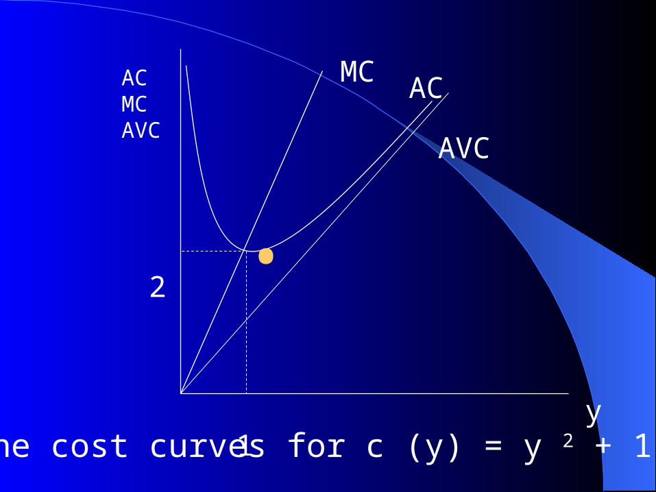
Typical cost Typical cost curves. curves.

c (y) = y 2 + 1.

Example:

AC MCAVC

y

MC

AVC

AC

The cost curves for c (y) = y 2 + 1

. 2

1

LR and SR cost curves.

y

AC SAC=C(y1, k* )/y

LAC=C(y)/y

. y*

Short-run and long-run average costs

y

AC Short-run average cost curves

Long-run average cost

curves y*

Short-run and long-run average costs

are costs that are not recoverable.

A special kind of fixed costs.

Sunk costs

Chapter 22Chapter 22

Firm Supply

Pure Pure competitioncompetition. .

Price Taker..

The demand curve facing a competitive firm. p380

Q

P

P*

Market price

Demand curve facing firm

Market demand

The supply decision:The supply decision:

FOC: MC ( y* ) = p.

SOC: MC ’ ( y* ) ≥ 0.

The The firm’s supply curvefirm’s supply curve is is the upward-sloping part of MCthe upward-sloping part of MC that lies above the AVC curve. that lies above the AVC curve.

The part of MC is also seen as the inverse supply function.

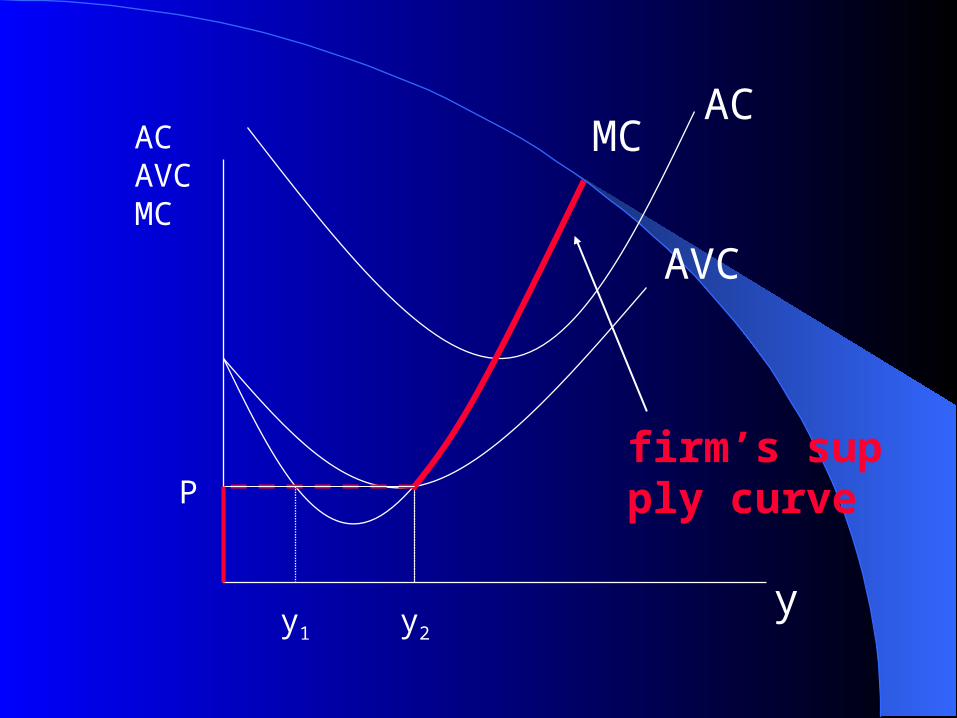
MC

AVC

AC

y

ACAVCMC

P

y2 y1

firm’s supply curve

Three Three equivalent waysequivalent ways to to measure the producer’s surplus measure the producer’s surplus

( = R – VC =π + FC ).( = R – VC =π + FC ). p389p389

P389 Example:

c ( y ) = y 2 + 1.

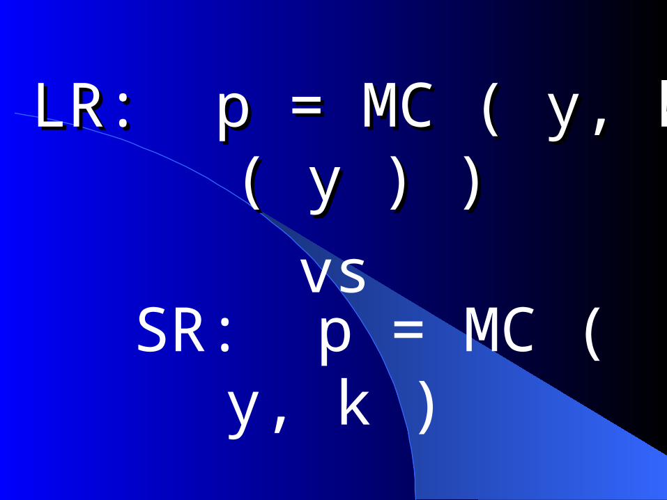
LR: p = MC ( y, k ( y ) )LR: p = MC ( y, k ( y ) )

vs

SR: p = MC ( y, k )

Chapter 23Chapter 23

Industry Supply

Horizontal summation Horizontal summation gives gives

the industry supply.

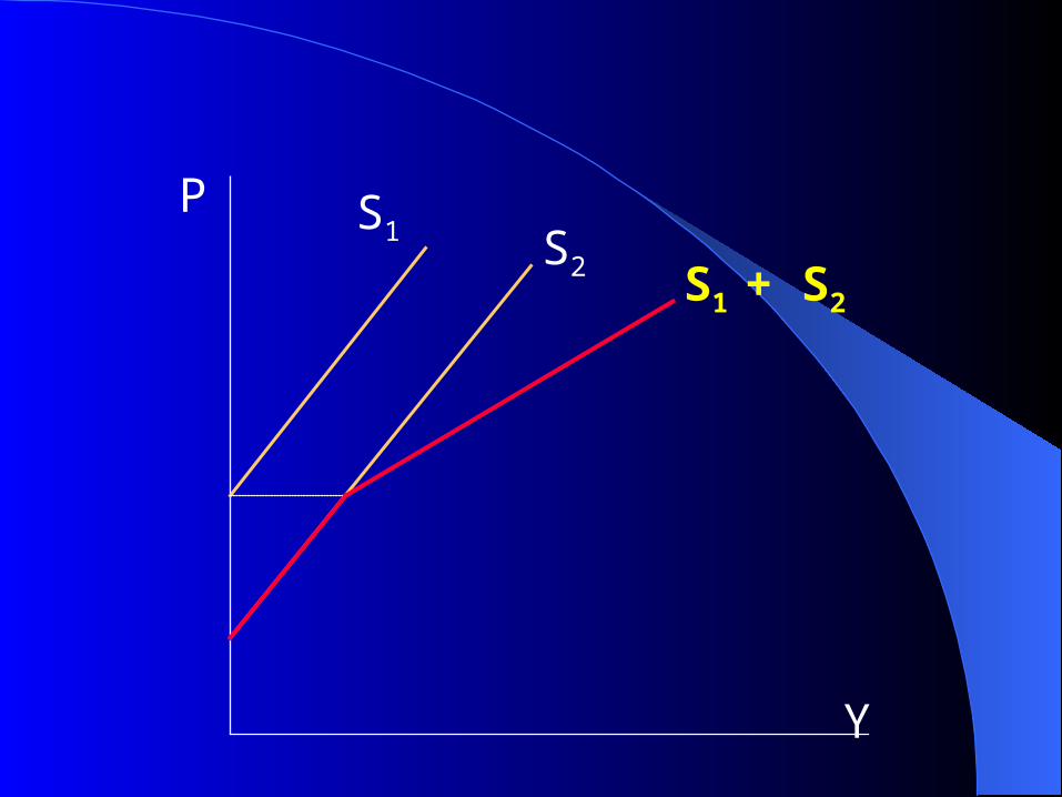
Y

P S1 S2 S1 + S2

Entry and Entry and exit. exit.

The The “zero profit” “zero profit” theorem theorem..

Free entryFree entry vs vs

barriers to entry. barriers to entry.

Economists Economists versus versus lobbyistslobbyists

Rent seeking.Rent seeking.