Chapter 4 structure design and analysis

B BRIDGE DESIGN PRACTICE ● AUGUST 2012

Chapter 4 – Structural Modeling and Analysis 4-i

CHAPTER 4

STRUCTURAL MODELING AND ANALYSIS

TABLE OF CONTENTS

4.1 INTRODUCTION ........................................................................................................... 4-1

4.2 STRUCTURE MODELING ........................................................................................... 4-1

4.2.1 General ............................................................................................................... 4-1

4.2.2 Structural Modeling Guidelines ......................................................................... 4-5

4.2.3 Material Modeling Guidelines ............................................................................ 4-7

4.2.4 Types of Bridge Models ..................................................................................... 4-7

4.2.5 Slab-Beam Bridges ............................................................................................. 4-9

4.2.6 Abutments ........................................................................................................ 4-14

4.2.7 Foundation ........................................................................................................ 4-15

4.2.8 Examples .......................................................................................................... 4-17

4.3 STRUCTURAL ANALYSIS ........................................................................................ 4-26

4.3.1 General ............................................................................................................. 4-26

4.3.2 Analysis Methods ............................................................................................. 4-27

4.4 BRIDGE EXAMPLES – 3-D VEHICLE LIVE LOAD ANALYSIS ........................... 4-35

4.4.1 Background ...................................................................................................... 4-35

4.4.2 Moving Load Cases .......................................................................................... 4-36

4.4.3 Live Load Distribution For One And Two-Cell Box Girders Example ........... 4-38

NOTATION ............................................................................................................................... 4-51

REFERENCES .......................................................................................................................... 4-52


Chapter 4 – Structural Modeling and Analysis 4-ii

This page is intentionally left blank.


Chapter 4 – Structural Modeling and Analysis 4-1

CHAPTER 4

STRUCTURAL MODELING AND ANALYSIS

4.1 INTRODUCTION

Structural analysis is a process to analyze a structural system to predict its

responses and behaviors by using physical laws and mathematical equations. The

main objective of structural analysis is to determine internal forces, stresses and

deformations of structures under various load effects.

Structural modeling is a tool to establish three mathematical models, including

(1) a structural model consisting of three basic components: structural members or

components, joints (nodes, connecting edges or surfaces), and boundary conditions

(supports and foundations); (2) a material model; and (3) a load model.

This chapter summarizes the guidelines and principles for structural analysis and

modeling used for bridge structures.

4.2 STRUCTURE MODELING

4.2.1 General

For designing a new structure, connection details and support conditions shall be

made as close to the computational models as possible. For an existing structure

evaluation, structures shall be modeled as close to the actual as-built structural

conditions as possible. The correct choice of modeling and analysis tools/methods

depends on:

a) Importance of the structure

b) Purpose of structural analysis

c) Required level of response accuracy

This section will present modeling guidelines and techniques for bridge

structures.

4.2.1.1 Types of Elements

Different types of elements may be used in bridge models to obtain characteristic

responses of a structure system. Elements can be categorized based on their principal

structural actions.

a) Truss Element

A truss element is a two-force member that is subjected to axial loads either

tension or compression. The only degree of freedom for a truss (bar) element is

axial displacement at each node. The cross sectional dimensions and material

properties of each element are usually assumed constant along its length. The

element may interconnect in a two-dimensional (2-D) or three-dimensional (3-D)

configuration. Truss elements are typically used in analysis of truss structures.



b) Beam Element

A beam element is a slender member subject to lateral loads and moments.

In general, it has six degrees of freedom at each node including translations and

rotations. A beam element under pure bending has only four degrees of freedom.

c) Frame Element

A frame element is a slender member subject to lateral loads, axial loads and

moments. It is seen to possess the properties of both truss and beam elements and

also called a beam-column element. A three-dimensional frame formulation

includes the effects of biaxial bending, torsion, axial deformation, and biaxial

shear deformations. A frame element is modeled as a straight line connecting two

joints. Each element has its own local coordinate system for defining section

properties and loads.

d) Plate Element

A plate element is a two dimensional solid element that acts like a flat plate.

There are two out-of-plane rotations and the normal displacement as Degree of

Freedom (DOF). These elements model plate-bending behavior in two

dimensions. The element can model the two normal moments and the cross

moment in the plane of the element. The plate element is a special case of a shell

element without membrane loadings.

e) Shell Element

A shell element (Figure 4.2-1) is a three-dimensional solid element (one

dimension is very small compared with another two dimensions) that carries

plate bending, shear and membrane loadings. A shell element may have either a

quadrilateral shape or a triangular shape. Shell element internal forces are

reported at the element mid-surface in force per unit length and are reported both

at the top and bottom of the element in force per unit area. It is primarily used to

determine local stress levels in cellular superstructure or in cellular pier and

caissons. It is generally recommended to use the full behavior unless the entire

structure is planar and is adequately restrained.

Figure 4.2-1 Shell and Solid Elements.



f) Plane Element

The plane element is a two-dimensional solid, with translational degrees of

freedom, capable of supporting forces but not moments. One can use either plane

stress elements or plane strain elements. Plane stress element is used to model

thin plate that is free to move in the direction normal to the plane of the plate.

Plane strain element is used to model a thin cut section of a very long solid

structure, such as walls. Plain strain element is not allowed to move in the normal

direction of the element’s plane (STRUDL Manual).

g) Solid Element

A solid element is an eight-node element as shown in Figure 4.2-1 for

modeling three-dimensional structures and solids. It is based upon an

isoparametric formulation that includes nine optional incompatible bending

modes. Solid elements are used in evaluation of principal stress states in joint

regions or complex geometries (CSI 2007).

h) The NlLink Element

A NlLink element (CSI 2007) is an element with structural nonlinearities. A

NlLink element may be either a one-joint grounded spring or a two-joint link and

is assumed to be composed of six separate springs, one for each degree of

deformational degrees of freedom including axial, shear, torsion, and pure

bending. Non-linear behavior is exhibited during nonlinear time-history analyses

or nonlinear static analyses.

4.2.1.2 Types of Boundary Elements

Selecting the proper boundary condition has an important role in structural

analysis. Effective modeling of support conditions at bearings and expansion joints

requires a careful consideration of continuity of each translational and rotational

component of displacement. For a static analysis, it is common to use a simpler

assumption of supports (i.e. fixed, pinned, roller) without considering the soil/

foundation system stiffness. However for dynamic analysis, representing the

soil/foundation stiffness is essential. In most cases choosing a [6×6] stiffness matrix

is adequate.

For specific projects, the nonlinear modeling of the system can be achieved by

using nonlinear spring/damper. Some Finite Element programs such as ADINA

(ADINA 2010) have more capability for modeling the boundary conditions than

others.

4.2.1.3 Types of Materials

Different types of materials are used for bridge structure members such as

concrete, steel, prestressing tendons, etc. For concrete structures, see Article C5.4.1

and for steel structures see Article 6.4 of AASHTO-LRFD (AASHTO 2007).



The material properties that are usually used for an elastic analysis are: modulus

of elasticity, shear modulus, Poisson’s ratio, the coefficient of thermal expansion, the

mass density and the weight density. One should pay attention to the units used for

material properties.

4.2.1.4 Types of Loads

There are two types of loads in a bridge design:

Permanent Loads: Loads and forces that are assumed to be either constant upon

completion of construction or varying only over a long time interval (CA 3.2).

Such loads include the self weight of structure elements, wearing surface, curbs,

parapets and railings, utilities, locked-in force, secondary forces from post-

tensioning, force effect due to shrinkage and due to creep, and pressure from

earth retainments (CA 3.3.2).

Transient Loads: Loads and forces that can vary over a short time interval to the

lifetime of the structure (CA 3.2). Such loads include gravity loads due to

vehicular, railway and pedestrian traffic, lateral loads due to wind and water, ice

flows, force effect due to temperature gradient and uniform temperature, and

force effect due to settlement and earthquakes (CA 3.3.2).

BDP Chapter 3 discusses loads in details.

4.2.1.5 Modeling Discretization

Formulation of a mathematical model using discrete mathematical elements and

their connections and interactions to capture the prototype behavior is called

Discretization. For this purpose:

a) Joints/Nodes are used to discretize elements and primary locations in

structure at which displacements are of interest.

b) Elements are connected to each other at joints.

c) Masses, inertia, and loads are applied to elements and then transferred to

joints.

Figure 4.2-2 shows a typical model discretization for a bridge bent.



Figure 4.2-2 Model Discretization for Monolithic Connection.

4.2.2 Structural Modeling Guidelines

4.2.2.1 Lumped-Parameter Models (LPMs)

Mass, stiffness, and damping of structure components are usually combined

and lumped at discrete locations. It requires significant experience to

formulate equivalent force-deformation with only a few elements to represent

structure response.

For a cast-in-place prestressed (CIP/PS) concrete box girder superstructure, a

beam element located at the center of gravity of the box girder can be used.

For non-box girder structures, a detailed model will be needed to evaluate the

responses of each separate girder.

4.2.2.2 Structural Component Models (SCMs) - Common Caltrans Practice

Based on idealized structural subsystems/elements to resemble geometry of

the structure. Structure response is given as an element force-deformations

relationship.

Gross moment of inertia is typically used for non-seismic analysis of

concrete column modeling.

Effective moment of inertia can be used when analyzing large deformation

under loads, such as prestressing and thermal effects. Effective moment of

inertia is the range between gross and cracked moment of inertia. To

calculate effective moment of inertia, see AASHTO LRFD 5.7.3.6.2

(AASHTO 2007).



Cracked moment of inertia is obtained using section moment - curvature

analysis (e.g. xSection or SAP2000 Section Designer), which is the moment

of inertia corresponding to the first yield curvature. For seismic analysis,

refer to Seismic Design Criteria (SDC) 5.6 “Effective Section Properties”

(Caltrans 2010).

4.2.2.3 Finite Element Models (FEMs)

A bridge structure is discretized with finite-size elements. Element

characteristics are derived from the constituent structural materials

(AASHTO 4.2).

Figure 4.2-3 shows the levels of modeling for seismic analysis of bridge

structures.

Figure 4.2-3 Levels of Modeling for Seismic Analysis of Bridge

(Priestley, et al 1996).

The importance of the structure, experience of the designer and the level of

needed accuracy affects type of model, location of joints and elements within the

selected model, and number of elements/joints to describe geometry of the structure.

For example, a horizontally curved structure should be defined better by shell

elements in comparison with straight elements. The other factors to be considered

are:

a) Structural boundaries - e.g., corners

b) Changes in material properties

c) Changes in element sectional properties

d) Support locations

e) Points of application of concentrated loads - Frame elements can have in-

span loads



4.2.3 Material Modeling Guidelines

Material models should be selected based on a material’s deformation under

external loads. A material is called elastic, when it returns to its original shape upon

release of applied loads. Otherwise it is called an inelastic material.

For an elastic body, the current state of stress depends only on the current state of

deformation while, in an inelastic body, residual deformation and stresses remain in

the body even when all external tractions are removed.

The elastic material may show linear or nonlinear behavior. For linear elastic

materials, stresses are linearly proportional to strains (σ = Eє) as described by

Hooke’s Law. The Hooke’s Law is applicable for both homogeneous and isotropic

materials.

Homogeneous means that the material properties are independent of the

coordinates.

Isotropic means that the material properties are independent of the rotation of

the axes at any point in the body or structure. Only two elastic constants

(modulus of elasticity E and Poisson’s ratio ν) are needed for linear elastic

materials.

For a simple linear spring, the constitutive law is given as: Fs = kξ where ζ is the

relative extension or compression of the spring, while Fs and k represent the force in

the spring and the spring stiffness, respectively. Stiffness is the property of an

element which is defined as force per unit displacement.

For a nonlinear analysis, nonlinear stress-strain relationships of structural

materials should be incorporated.

For unconfined concrete a general stress-strain relationship proposed by

Hognestad is widely used. For confined concrete, generally Mander’s model

is used (Chen and Duan 1999).

For structural steel and reinforcing steel, the stress-strain curve usually

includes three segments: elastic, perfectly plastic, and a strain-hardening

region.

For prestressing steel, an idealized nonlinear stress-strain model may be

used.

4.2.4 Types of Bridge Models

4.2.4.1 Global Bridge Models

A global bridge model includes the entire bridge with all frames and connecting

structures. It can capture effects due to irregular geometry such as curves in plane and

elevation, effects of highly-skewed supports, contribution of ramp structures, frames

interaction, expansion joints, etc. It is primarily used in seismic design to verify

design parameters for the individual frame. The global model may be in question

because of spatially varying ground motions for large, multi-span, and multi-frame



bridges under seismic loading. In this case a detailed discretization and modeling

force-deformation of individual element is needed.

4.2.4.2 Tension and Compression Models

The tension and compression models are used to capture nonlinear responses for

bridges with expansion joints (MTD 20-4, Caltrans 2007) to model the non-linearity

of the hinges with cable restrainers. Maximum response quantities from the two

models are used for seismic design.

a) Tension Model

Tension model is used to capture out-of-phase frame movement. The tension

model allows relative longitudinal movement between adjacent frames by

releasing the longitudinal force in the rigid hinge elements and abutment joints

and activating the cable restrainer elements. The cable restrainer unit is modeled

as an individual truss element with equivalent spring stiffness for longitudinal

movement connecting across expansion joints.

b) Compression Model

Compression model is used to capture in-phase frame movement. The

compression model locks the longitudinal force and allows only moment about

the vertical and horizontal centerline at an expansion joint to be released. All

expansion joints are rigidly connected in longitudinal direction to capture effects

of joint closing-abutment mobilized.

4.2.4.3 Frame Models

A frame model is a portion of structure between the expansion joints. It is a

powerful tool to assess the true dynamic response of the bridge since dynamic

response of stand-alone bridge frames can be assessed with reasonable accuracy as an

upper bound response to the whole structure system. Seismic characteristics of

individual frame responses are controlled by mass of superstructure and stiffness of

individual frames. Transverse stand-alone frame models shall assume lumped mass at

the columns. Hinge spans shall be modeled as rigid elements with half of their mass

lumped at the adjacent column (SDC Figure 4.2, Caltrans 2010). Effects from the

adjacent frames can be obtained by including boundary frames in the model.

4.2.4.4 Bent Models

A transverse model of bent cap and columns is needed to obtain maximum

moments and shears along bent cap. Dimension of bent cap should be considered

along the skew.

Individual bent model should include foundation flexibility effects and can be

combined in frame model simply by geometric constraints. Different ground motion

can be input for individual bents. The high in-plane stiffness of bridge superstructures

allows rigid body movement assumption which simplifies the combination of

individual bent models.



4.2.5 Slab-Beam Bridges

4.2.5.1 Superstructures

For modeling slab-beam bridges, either Spine Model or a Grillage Model should

be used.

Figure 4.2-4 Superstructure Models (Priestley, et al 1996).

a) Spine Model

Spine Models with beam elements are usually used for ordinary bridges.

The beam element considers six DOF at both ends of the element and is

modeled at their neutral axis.

The effective stiffness of the element may vary depending on the

structure type.

Use SDC V1.6 to define effective flexural stiffness EIeff for

reinforced concrete box girders and pre-stressed box girders as

follows:

For reinforced concrete (RC) box girder, (0.5~0.75) EIg

For prestressed concrete (PS) box girder, 1.0 EIg and for tension

it considers Ig,

where Ig is the gross section moment of inertia.

The torsional stiffness for superstructures can be taken as: GJ for un-

cracked section and 0.5 GJ for cracked section.

Spine model can’t capture the superstructure carrying wide roadway,

high-skewed bridges. In these cases use grillage model.



b) Grillage Models/3D Finite Element Model

Grillage Models are used for modeling steel composite deck

superstructures and complicated structures where superstructures

can’t be considered rigid such as very long and narrow bridges,

interchange connectors.

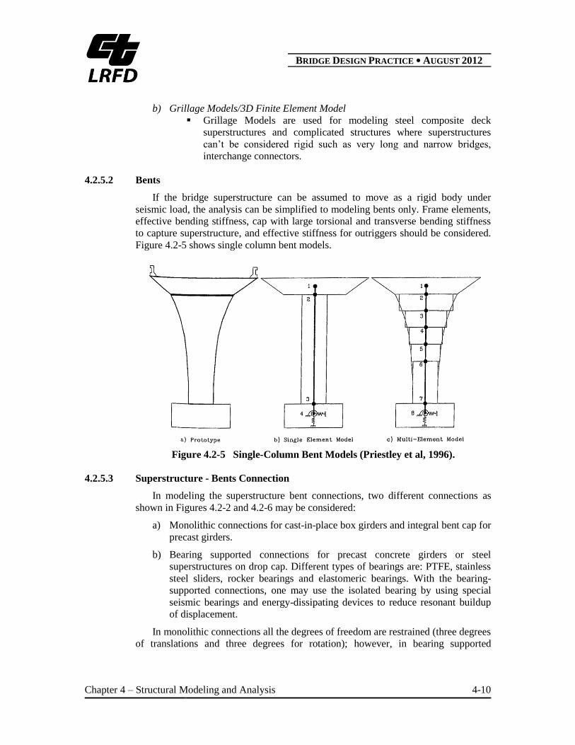
4.2.5.2 Bents

If the bridge superstructure can be assumed to move as a rigid body under

seismic load, the analysis can be simplified to modeling bents only. Frame elements,

effective bending stiffness, cap with large torsional and transverse bending stiffness

to capture superstructure, and effective stiffness for outriggers should be considered.

Figure 4.2-5 shows single column bent models.

Figure 4.2-5 Single-Column Bent Models (Priestley et al, 1996).

4.2.5.3 Superstructure - Bents Connection

In modeling the superstructure bent connections, two different connections as

shown in Figures 4.2-2 and 4.2-6 may be considered:

a) Monolithic connections for cast-in-place box girders and integral bent cap for

precast girders.

b) Bearing supported connections for precast concrete girders or steel

superstructures on drop cap. Different types of bearings are: PTFE, stainless

steel sliders, rocker bearings and elastomeric bearings. With the bearing-

supported connections, one may use the isolated bearing by using special

seismic bearings and energy-dissipating devices to reduce resonant buildup

of displacement.

In monolithic connections all the degrees of freedom are restrained (three degrees

of translations and three degrees for rotation); however, in bearing supported



connections, only three degrees of translations are restrained but the rotational

degrees of freedom are free.

In the bearing supported structures, the superstructure is not subjected to seismic

moment transferred through the column. However the design is more sensitive to

seismic displacement than with the monolithic connection.

The energy dissipation devices in the isolated bearing reduce the seismic

displacement significantly in comparison with bearing-supported structures. The

designer should pay attention to the possibility of increased acceleration when using

the bearing-supported connections with or without energy-dissipation devices in soft

soils.

Figure 4.2-6 Superstructure-Bent Connection.

4.2.5.4 Hinges

Hinges separate frames in long structures to allow for movements due to thermal,

initial pre-stress shortening and creep without large stresses and strains in members.

A typical hinge should be modeled as 6 degrees of freedom, i.e., free to rotate in

the longitudinal direction and pin in the transverse direction to represent shear

(Figure 4.2-7).



It is Caltrans practice to use Linear Elastic Modal Analysis with two different

structural models, Tension and Compression, to take care of this analysis issue.

Figure 4.2-7 Span Hinge Force Definitions (Priestley et al, 1996).

4.2.5.5 Substructures

Figures 4.2-8 and 4.2-9 show a multi-column bent model and a foundations

spring model at a bent, respectively. Figure 4.2-10 shows a multi bridge frame model.

a) Column-Pier Sections

Prismatic - same properties or Non-Prismatic

Shapes Circular Column, Rectangular, Hollow-Section Column

Figure 4.2-8 Multi-Column Bent Model (Priestley et al, 1996).



b) Bent-Foundation Connection

Pin base: Generally used for multi-column bents.

Fixed Base: For single column base.

Figure 4.2-9 Foundation Spring Definition at a Bent.



Figure 4.2-10 Multi Bridge Frame (Priestley et al, 1996).

4.2.6 Abutments

When modeling bridge structure, abutment can be modeled as pin, roller or fixed

boundary condition. For modeling the soil-structure interaction, springs can be used.



Figure 4.2-11 shows end restraint with springs to model soil-structure interaction for

seat and rigid abutments. Abutment stiffness, capacities, and damping affect seismic

response. Seismic Design Criteria V1.6, Section 7-8 discusses the longitudinal and

transverse abutment responses in an earthquake. For modeling gap, back wall and

piles effective stiffness is used with non-linear behavior. Iterative procedure should

be used to find a convergence between stiffness and displacement.

Figure 4.2-11 Foundation Spring Definition.

4.2.7 Foundation

4.2.7.1 Group Piles

Supports can be modeled using:

Springs - 6 × 6 stiffness matrix - defined in global/joint local coordinate

system.

Restraints - known displacement, rotation - defined in global DOF.

Complete pile system with soil springs along with the bridge.



4.2.7.2 Pile shaft

When modeling the pile shaft for non-seismic loading, an equivalent fixity model

can be used (Figure 4.2-12c). For seismic loading, a soil-spring model (Figure 4.2-

12b) should be considered to capture the soil-structure interaction. Programs such as

Wframe, L-Pile, SAP2000/CSI or ADINA can be used.

a) Prototype b) Soil-Spring Model c) Equivalent Fixity Model

Figure 4.2-12 CIDH Pile Shaft Models (Priestley et al, 1996).

4.2.7.3 Spread Footing

Spread footings are usually built on stiff and competent soils, fixed boundary

conditions are assumed for the translational springs, and rotation is considered only

when uplift and rocking of the entire footing are expected.



4.2.8 Examples

4.2.8.1 CTBridge

CTBridge is a Finite Element Analysis and Design software using a 3D spine

model for the bridge structure. This allows description of skewed supports, horizontal

and vertical curves, and multi-column bents.

CTBridge allows user manipulation of various settings such as:

Number of Elements

Live Load Step Sizes

Prestress Discretization

P-Jack Design Limits

For non-skewed bridges, the abutment can be considered pinned or roller. For

skewed bridges, springs should be used at the abutments. The stiffness of the springs

shall be based on the stiffness of the bearing pads. If bearing stiffness is not available,

slider can be used instead of pin or roller. For bridges with curved alignments and

skewed supports or straight bridges with skews in excess of 60 degrees, a full 3-D

analysis model, such as a grillage or shell model may be required to more accurately

capture the true distribution of the load.

Note that in order to get the result at each 0.1 span, you should define the offset

from begin and end span, i.e. from CL abutment to face of abutment.

The following structure shown in Figures 4.2-13a to 4.2-13c is used as an

example for CTBridge.

Figure 4.2-13a Elevation View of Example Bridge.



Figure 4.2-13b Typical Section View of Example Bridge.

Figure 4.2-13c Plan View of Example Bridge.



Figure 4.2-14 shows CTBridge model for example bridge.

Figure 4.2-14 Example Bridge - CTBridge Model.

Figure 4.2-15 shows sign convention for CTBridge.

Figure 4.2-15 Sign Convention at CTBridge.



Figure 4.2-16 shows two spine models.

Figure 4.2-16 3D Frame in CTBridge.

4.2.8.2 SAP2000/CSI

SAP2000/CSI is the latest and one of the most powerful versions of the well-

known Finite Element Program SAP series of Structural Analysis Programs, which

offers the following features:

Static and Dynamic Analysis

Linear and Nonlinear Analysis

Dynamic Seismic Analysis and Static Pushover Analysis

Vehicle Live-Load Analysis for Bridges, Moving Loads with 3D Influence

Surface, Moving Loads with Multi-Step Analysis, Lane Width Effects

P-Delta Analysis

Cable Analysis

Eigen and Ritz Analyses

Fast Nonlinear Analysis for Dampers

Energy Method for Drift Control

Segmental Construction Analysis



The following are the general steps to be defined for analyzing a structure using

SAP2000/CSI:

Geometry (input nodes coordinates, define members and connections)

Boundary Conditions/ Joint Restraints (fixed, free, roller, pin or partially

restrained with a specified spring constant)

Material Property (Elastic Modulus, Poisson’s Ratio, Shear Modulus,

damping data, thermal properties and time-dependent properties such as

creep and shrinkage)

Loads and Load cases

Stress-strain relationship

Perform analysis of the model based on analysis cases

Bridge Designers can use SAP2000/CSI Bridge templates for generating Bridge

Models, Automated Bridge Live Load Analysis and Design, Bridge Base Isolation,

Bridge Construction Sequence Analysis, Large Deformation Cable Supported Bridge

Analysis, and Pushover Analysis.

The user can either model the structure as a Spine Model (Frame) or a 3D Finite

Element Model.

Concrete Box Girder Bridge:

In this section, we create a SAP2000/CSI model for the Example Bridge

using the Bridge Wizard (BrIM-Bridge Information Modeler). The Bridge

Modeler has 13 modeling step processes which are described below:

a) Layout line

The first step in creating a bridge object is to define highway layout lines

using horizontal and vertical curves. Layout lines are used as reference lines

for defining the layout of bridge objects and lanes in terms of stations,

bearings and grades considering super elevations and skews.

b) Deck Section

Various parametric bridge sections (Box Girders & Steel Composites)

are available for use in defining a bridge. See Figure 4.2-17.

User can specify different Cross Sections along Bridge length.



Figure 4.2-17 Various Bridge Sections.

c) Abutment Definition

Abutment definitions specify the support conditions at the ends of the

bridge. The user defined support condition allows each six DOF at the

abutment to be specified as fixed, free or partially restrained with a specified

spring constant.

Those six Degrees of Freedom are:

U1- Translation Parallel to Abutment

U2- Translation Normal to Abutment

U3- Translation Vertical

R1- Rotation about Abutment

R2- Rotation About Line Normal to Abutment

R3- Rotation about Vertical

For Academy Bridge consider U2, R1 and R3 DOF directions to have a

“Free” release type and other DOF fixed.

d) Bent Definition

This part specifies the geometry and section properties of bent cap beam

and bent cap columns (single or multiple columns) and base support

condition of the bent columns.



The base support condition for a bent column can be fixed, pinned or

user defined as a specified link/support property which allows six degrees of

freedom.

For Example Bridge enter the column base supports as pinned. All units

should be kept consistent (kip-ft for this example).

The locations of columns are defined as distance from left end of the cap

beam to the centerline of the column and the column height is the distance

from the mid-cap beam to the bottom of the column.

For defining columns use Bent definition under bridge wizard, then go to

Define/show bents and go to Modify/show column data. The base column

supports at top and bottom will be defined here.

e) Diaphragm Definition

Diaphragm definitions specify properties of vertical diaphragms that

span transverse across the bridge. Diaphragms are only applied to area

objects and solid object models and not to spine models. Steel diaphragm

properties are only applicable to steel bridge sections.

f) Hinge Definition

Hinge definitions specify properties of hinges (expansion joints) and

restrainers. After a hinge is defined, it can be assigned to one or more spans

in the bridge object.

A hinge property can be a specified link/support property or it can be

user-defined spring. The restrainer property can be also a link/support or user

defined restrainer. The user-restrainer is specified by a length, area and

modulus of elasticity.

g) Parametric Variation Definition

Any parameter used in the parametric definition of the deck section can

be specified to vary such as bridge depth, thickness of the girders and slabs

along the length of the bridge. The variation may be linear, parabolic or

circular.

h) Bridge Object Definition

The main part of the Bridge Modeler is the Bridge Object Definition

which includes defining bridge span, deck section properties assigned to each

span, abutment properties and skews, bent properties and skews, hinge

locations are assigned, super elevations are assigned and pre-stress tendons

are defined.

The user has two tendon modeling options for pre-stress data:

Model as loads

Model as elements



Since we calculate the pre-stress jacking force from CTBridge, use

option(a) to input the Tendon Load force. The user can input the Tendon loss

parameters which have two parts:

1) Friction and Anchorage losses (Curvature coefficient, Wobble

coefficient and anchorage setup).

2) Other loss parameters (Elastic shortening stress, Creep stress,

Shrinkage stress and Steel relaxation stress).

When you input values for Friction and Anchorage losses, make sure the

values match your CTBridge which should be based on “CALIFORNIA

Amendments Table 5.9.5.2.2b-1 (Caltrans 2008) and there is no need to input

other loss parameters. If the user decides to model tendon as elements, the

values for other loss parameters shall be input; otherwise, leave the default

values.

Note: If you model the bridge as a Spine Model, only define one single

tendon with total Pjack load. If you model the bridge with shell

element, then you need to specify tendon in each girder and input the

Pjack force for each girder which should be calculated as Total Pjack

divided by number of the girders.

Note: Anytime a bridge object definition is modified, the link model must be

updated for the changes to appear in SAP2000/CSI model.

i) Update Linked Model

The update linked model command creates the SAP2000/CSI object-

based model from the bridge object definition. Figures 4.2-18 and 4.2-19

show an area object model and a solid object model, respectively. Note that

an existing object will be deleted after updating the linked model. There are

three options in the Update Linked Model including:

Update a Spine Model using Frame Objects

Update as Area Object Model

Update as Solid Object Model



Figure 4.2-18 Area Object Model.

Figure 4.2-19 Solid Object Model.

Parametric Bridge Modeling

Layered Shell Element

Lane Definition Using Highway Layout or Frame Objects

Automatic Application of Lane Loads to Bridge

Predefined Vehicle and Train Loads

Bridge Results & Output

Influence Lines and Surfaces

Forces and Stresses Along and Across Bridge



Displacement Plots

Graphical and Tabulated Outputs

SAP2000/CSI also has an Advanced Analysis Option that is not discussed in this

section including:

Segmental Construction

Include the Effects of Creep, Shrinkage Relaxation

Pushover Analysis using Fiber Models

Bridge Base Isolation and Dampers

Explicitly Model Contact Across Gaps

Nonlinear Large Displacement Cable Analysis

Line and Surface Multi-Linear Springs (P-y curves)

High Frequency Blast Dynamics using Wilson FNA

Nonlinear Dynamic Analysis & Buckling Analysis

Multi-Support Seismic Excitation

Animated Views of Moving Loads

The program has the feature of automated line constraints that enforce the

displacement compatibility along the common edges of meshes as needed.

4.3 STRUCTURAL ANALYSIS

Structural Analysis provides the numerical mathematical process to extract

structure responses under service and seismic loads in terms of structural demands

such as member forces and deformations.

4.3.1 General

For any type of structural analysis, the following principles should be considered.

4.3.1.1 Equilibrium

a) Static Equilibrium

In a supported structure system when the external forces are in balance with the

internal forces, or stresses, which exactly counteract the loads (Newton’s Second

Law), the structure is said to be in equilibrium.

Since there is no translatory motion, the vector sum of the external forces must

be zero ( 0F ). Since there is no rotation, the sum of the moments of the external

forces about any point must be zero ( 0M ).

b) Dynamic Equilibrium

When dynamic effects need to be included, whether for calculating the dynamic

response to a time-varying load or for analyzing the propagation of waves in a

structure, the proper inertia terms shall be considered for analyzing the dynamic

equilibrium:

F mu



4.3.1.2 Constitutive Laws

The constitutive laws define the relationship between the stress and strain in the

material of which a structure member is made.

4.3.1.3 Compatibility

Compatibility conditions are referred to continuity or consistency conditions on

the strains and the deflections. As a structure deforms under a load, we want to

ensure that:

a) Two originally separate points do not merge into a same point.

b) Perimeter of a void does not overlap as it deforms.

c) Elements connected together remain connected as the structure deforms.

4.3.2 Analysis Methods

Different types of analysis are discussed in this section.

4.3.2.1 Small Deflection Theory

If the deformation of the structure doesn’t result in a significant change in force

effects due to an increase in the eccentricity of compressive or tensile forces, such

secondary force effects may be ignored. Small deflection theory is usually adequate

for the analyses of beam-type bridges. Suspension bridges, very flexible cable-stayed

bridges and some arches rather than tied arches and frames in which flexural

moments are increased by deflection are generally sensitive to deflections. In many

cases the degree of sensitivity can be evaluated by a single-step approximate method,

such as moment magnification factor method (AASHTO 4.5.3.2.2).

4.3.2.2 Large Deflection Theory

If the deformation of the structure results in a significant change in force effects,

the effects of deformation shall be considered in the equations of equilibrium. The

effect of deformation and out-of-straightness of components shall be included in

stability analysis and large deflection analyses. For slender concrete compressive

components, time-dependent and stress-dependent material characteristics that cause

significant changes in structural geometry shall be considered in the analysis.

Because large deflection analysis is inherently nonlinear, the displacements are

not proportional to applied load, and superposition cannot be used. Therefore, the

order of load application are very important and should be applied in the order

experienced by the structure, i.e. dead load stages followed by live load stages, etc. If

the structure undergoes nonlinear deformation, the loads should be applied

incrementally with consideration for the changes in stiffness after each increment.



4.3.2.3 Linear Analysis

In the linear relation of stress-strain of a material, Hooke’s law is valid for small

stress-strain range. For linear elastic analysis, sets of loads acting simultaneously can

be evaluated by superimposing (adding) the forces or displacements at the particular

point.

4.3.2.4 Non-linear Analysis

The objective of non-linear analysis is to estimate the maximum load that a

structure can support prior to structural instability or collapse. The maximum load

which a structure can carry safely may be calculated by simply performing an

incremental analysis using non-linear formulation. In a collapse analysis, the

equation of equilibrium is for each load or time step.

Design based on assumption of linear stress-strain relation will not always be

conservative due to material or physical non-linearity. Very flexible bridges, e.g.

suspension and cable-stayed bridges, should be analyzed using nonlinear elastic

methods (LRFD C4.5.1, AASHTO 2007).

P-Delta effect is an example of physical (geometrical) non-linearity, where

principle of superposition doesn’t apply since the beam-column element undergoes

large changes in geometry when loaded.

4.3.2.5 Elastic Analysis

Service and fatigue limit states should be analyzed as fully elastic, as should

strength limit states, except in the case of certain continuous girders where inelastic

analysis is permitted, inelastic redistribution of negative bending moment and

stability investigation (LRFD C4.5.1, AASHTO 2007).

When modeling the elastic behavior of materials, the stiffness properties of

concrete and composite members shall be based upon cracked and/or uncracked

sections consistent with the anticipated behavior (LRFD 4.5.2.2, AASHTO 2007). A

limited number of analytical studies have been performed by Caltrans to determine

effects of using gross and cracked moment of inertia. The specific studies yielded the

following findings on prestressed concrete girders on concrete columns:

1) Using Igs or Icr in the concrete columns do not significantly reduce or increase

the superstructure moment and shear demands for external vertical loads, but

will significantly affect the superstructure moment and shear demands from

thermal and other lateral loads (CA C4.5.2.2, Caltrans 2008). Using Icr in the

columns can increase the superstructure deflection and camber calculations

(CA 4.5.2.2, Caltrans 2008).

Usually an elastic analysis is sufficient for strength-based analysis.



4.3.2.6 Inelastic Analysis

Inelastic analysis should be used for displacement-based analysis (Chen and

Duan 1999).

The extreme event limit states may require collapse investigation based entirely

on inelastic modeling. Where inelastic analysis is used, a preferred design failure

mechanism and its attendant hinge locations shall be determined (LRFD 4.5.2.3,

AASHTO 2007).

4.3.2.7 Static Analysis

Static analysis mainly used for bridges under dead load, vehicular load, wind

load and thermal effects. The influence of plan geometry has an important role in

static analysis (AASHTO 4.6.1). One should pay attention to plan aspect ratio and

structures curved in plan for static analysis.

Plan Aspect Ratio

If the span length of a superstructure with torsionally stiff closed crossed

section exceeds 2.5 times its width, the superstructure may be idealized as a

single-spine beam. Simultaneous torsion, moment, shear and reaction forces and

the attendant stresses are to be superimposed as appropriate. In all equivalent

beam idealizations, the eccentricity of loads should be taken with respect to the

centerline of the equivalent beam.

Structure curved in plan

Horizontally cast-in-place box girders may be designed as single spine beam

with straight segments, for central angles up to 34° within one span, unless

concerns about other force effects dictate otherwise. For I-girders, since

equilibrium is developed by the transfer of load between the girders, the analysis

must recognize the integrated behavior of all structure components.

Small deflection theory is adequate for the analysis of most curved-girder

bridges. However curved I-girders are prone to deflect laterally if not sufficiently

braced during erection. This behavior may not be well recognized by small deflection

theory.



4.3.2.8 Equivalent Static Analysis (ESA)

It is used to estimate seismic demands for ordinary bridge structures as specified

in Caltrans SDC (Caltrans 2010). A bridge is usually modeled as Single-Degree-of-

Freedom (SDOF) and seismic load applied as equivalent static horizontal force. It is

suitable for individual frames with well balanced spans and stiffness. Caltrans SDC

(Caltrans 2010) recommends stand-alone “Local” Analysis in Transverse &

Longitudinal direction for demands assessment. Figure 4.3-1 shows a stand-alone

model with lumped masses at columns, rigid body rotation, and half span mass at

adjacent columns.

Transverse Stand-Alone Model

Longitudinal Stand-Alone Model

Figure 4.3-1 Stand Alone Model.

Types of Equivalent Static Analysis such as Lollipop Method, Uniform Load

Method and Generalized Coordinate Method can be used.

4.3.2.9 Nonlinear Static Analysis (Pushover Analysis)

Nonlinear Incremental Static Procedure is used to determine displacement

capacity of a bridge structure.

Horizontal loads are incrementally increased until a structure reaches collapse

condition or collapse mechanism. Change in structure stiffness is modeled as member

stiffness due to cracking, plastic hinges, yielding of soil spring at each step (event).



Analysis Programs are available such as: WFRAME, SAP2000/CSI, STRUDL,

SC-Push 3D, ADINA.

Figures 4.3-2 and 4.3-3 shows typical road-displacement and moment-curative

for a concrete column.

Figure 4.3-2 Pushover curve.

a) Pushover Analysis - Requirements

Linear Elastic Structural Model

Initial or Gravity loads

Characterization of all Nonlinear actions - multi-linear force-deformation

relationships (e.g. plastic hinge moment-curvature relationship)

Limits on strain based on design performance level to compute moment

curvature relationship of nonlinear hinge elements.

Section Analysis─> Strain─> Curvature

Double Integration of curvature─> Displacements

Track design performance level strain limits in structural response

Figure 4.3-3 A Typical Moment-Curvature Curve for a Concrete Column.

4.3.2.10 General Dynamic Equilibrium Equation

The dynamic equation of motion for a typical SDOF is:



Input I D S

F F F F

Where:

F1 = mass × acceleration = mü

FD = Damping const × Velocity = mu

FS = Stiffness Deformation = ku

m = mass =ρs

WeightV

g

s = Material mass density

V = Element volume = A L

K = stiffness

c = damping constant = z ccr

ccr = critical damping = 2 m w

z = damping-ratio =2

0.5 p EDC

ku

EDC = Energy dissipated per cycle

U = displacement

Besides earthquake, wind and moving vehicles can cause dynamic loads on

bridge structures.

Wind load may induce instability and excessive vibration in long-span bridges.

The interaction between the bridge vibration and wind results in two kind of forces:

motion-dependent and motion-independent. The motion dependent force causes

aerodynamic instability with emphasis on vibration of rigid bodies. For short span

bridges the motion dependent part is insignificant and there is no concern about

aerodynamic instability. The bridge aerodynamic behavior is controlled by two types

of parameters: structural and aerodynamics. The structure parameters are the bridge

layout, boundary condition, member stiffness, natural modes and frequencies. The

aerodynamic parameters are wind climate, bridge section shape. The aerodynamic

equation of motion is expressed as:

md mimü cu ku FU F

Where:

FUmd = motion-dependent aerodynamic force vector

Fmi = motion-independent wind force vector

For a detailed analytical solution for effect of wind on long span bridges and

cable vibration, see (Chen and Duan 1999).

4.3.2.11 Free Vibration Analysis

Vehicles such as trucks and trains passing bridges at certain speed will cause

dynamic effects. The dynamic loads for moving vehicles on bridges are counted for

by a dynamic load allowance, IM. See (Chen and Duan 1999).



Major characteristics of the bridge dynamic response under moving load can be

summarized as follows:

Impact factor increases as vehicle speed increases, impact factor decreases as

bridge span increases.

Under the condition of “Very good” road surface roughness (amplitude of

highway profile curve is less than 0.4 in.) the impact factor is well below the design

specifications. But the impact factor increases tremendously with increasing road

surface roughness from “good” to “poor” (the amplitude of the roadway profile is

more than 1.6 in.) beyond the impact factor specified in AASHTO LRFD

Specifications.

Field tests indicate that in the majority of highway bridges, the dynamic

component of the response does not exceed 25% of the static response to vehicles

with the exception of deck joints. For deck joints, 75% of the impact factor is

considered for all limit states due to hammer effect, and 15% for fatigue and fracture

limit states for members vulnerable to cyclic loading such as shear connectors, see

CA - C3.6.2.1 (Caltrans 2008) to AASHTO LRFD (AASHTO 2007).

Dynamic effects due to moving vehicles may be attributed to two sources:

Hammering effect is the dynamic response of the wheel assembly to riding

surface discontinuities, such as deck joints, cracks, potholes and

delaminations.

Dynamic response of the bridge as a whole to passing vehicles, which may

be due to long undulations in the roadway pavement, such as those caused by

settlement of fill, or to resonant excitation as a result of similar frequencies

of vibration between bridge and vehicle. (AASHTO LRFD C3.6.2.1)

The magnitude of dynamic response depends on the bridge span, stiffness and

surface roughness, and vehicle dynamic characteristics such as moving speed and

isolation systems. There have been two types of analysis methods to investigate the

dynamic response of bridges due to moving load:

Numerical analysis (Sprung mass model).

Analytical analysis (Moving load model).

The analytical analysis greatly simplifies vehicle interaction with bridge and

models a bridge as a plate or beam with a good accuracy if the ratio of live load to

self weight of the superstructure is less than 0.3.

Free vibration analysis assuming a sinusoidal mode shape can be used for the

analysis of the superstructure and calculating the fundamental frequencies of slab-

beam bridges (Chen and Duan 1999).

For long span bridges or low speed moving load, there is little amplification

which does not result in much dynamic responses.

Maximum dynamic response happens when load frequency is near the bridge

fundamental frequency.



The aspect ratios of the bridge deck play an important role. When they are less

than 4.0 the first mode shape is dominant, when more than 8.0, other mode shapes are

excited.

Free-Vibration Properties are shown in Figure 4.3-4.

Figure 4.3-4 Natural Period.

a) Cycle: When a body vibrates from its initial position to its extreme positive

position in one direction, back to extreme negative position, and

back to initial position (i.e., one revolution of angular displacement

of 2 ) (radians)

b) Frequency ( ): If a system is disturbed and allowed to vibrate on its own,

without external forces and damping (free Vibration).

A system having n degrees of freedom will have, in general, n distinct natural

frequencies of vibration.

K / mω

¼ cycles

T/2

T = 2 sec

f = 1/T = ½ = 0.5 cycle/sec

= 2* /T = rad/sec

T = 1sec

f = 1/T = 1/1= 1.0

cycle/sec

= 2* /T = 2* rad/sec

T = 0.5 sec

f = 1/T = 1/0.5= 2.0 cycle/sec

= 2* /T = 4* rad/sec

T

T

T

K

m

0

2*

/2

2* /3

R=1.

2ω distance/time

T



ω 2 f

c) Period (T): Is the time taken to complete one cycle of motion. It is equal to

the time required for a vector to rotate 2 (one round)

d) Frequency (f): The number of cycles per unit time, f = 1/T (H.Z)

4.4 BRIDGE EXAMPLES – 3-D VEHICLE LIVE LOAD

ANALYSIS

4.4.1 Background

The United States has a long history of girder bridges being designed “girder-by-

girder”. That is, the girder is designed for some fraction of live loads, depending on

girder spacing and structure type. The method is sometimes referred to as “girder

line” or “beam line” analysis and the fraction of live load lanes used for design is

sometimes referred to as a grid or Load Distribution Factor (LDF).

The approximate methods of live-load distribution in the AASHTO LRFD Bridge

Design Specifications (AASHTO 2007) use “girder load distribution factors” (LDFs)

to facilitate beam analysis of multiple vehicular live loads on a three-dimensional

bridge structural system. The formal definition of LDF: “a factor used to multiply the

total longitudinal response of the bridge due to a single longitudinal lane load in

order to determine the maximum response of a single girder” (Barker and Puckett

2007). A more practical definition: the ratio Mrefined /Mbeam or Vrefined /Vbeam, where the

numerator is the enveloped force effect at one location, and the denominator is force

effect at the same location in a single girder due to the same load.

Although each location within a girder can have a different LDF, the

expressions in the tables of AASHTO LRFD BRIDGE SPECIFICATIONS,

Articles 4.6.2.2.2 and 4.6.2.2.3 are based on the critical locations for bending

and shear, respectively. Critical locations refer to maximum absolute

positive moments, negative moments, and maximum absolute shear. For

cast-in-place (CIP) concrete multicell box girders, the AASHTO tables only

apply to typical bridges, which refer to:

Girder spacing, S: 6′ < S < 13′

Span length, L: 60′ < L < 220′

Structure depth, D: 35″ < d < 110″

The use of approximate methods on less-typical structures is prohibited. The

less-typical structures refer to either one of the following cases:

One or two-cell box girders;

Two or three-girder beam-slab structures;

Spans greater than 240 ft in length;



Structures with extra-wide overhangs (greater than one-half of the girder

spacing or 3 ft).

Three-dimensional (3D) finite element analysis (FEA) must be used to

determine the girder LDFs of these less-typical bridges. The following cases

may also require such refined analysis:

Skews greater than 45 ;

Structures with masonry sound walls;

Beam-slab structures with beams of different bending stiffness.

A moving load analysis on a 3D finite element (FE) model provides accurate

load distribution. However, for routine design of commonly used bridge

superstructure system, 3D FEA requires the familiarity with sophisticated,

usually also expensive, finite element methods.

FEM software. It may not be economical due to the additional time required

to build and run the 3D model, and analyze the results, comparing to simple

FEM program, e.g. Caltrans.

CTBridge. In addition, in terms of the reliability of an FE model, 3D FEM

model may not be as reliable as a simple 2D FE model due to the much

greater number of details in a 3D FE model. Based on Caltrans experience, a

combination of LDF formula with the in-house 2D FEM design program,

CTBridge, provides sufficient, reliable and efficient design procedure and

output. The latest version of CTBridge includes the LDF values for a one- or

two-cell box-girder bridge.

4.4.2 Moving Load Cases

In many situations, the one- or two-cell box girders are for widening of existing

bridges. If they are new bridges, it is also possible that they will be widened in the

future. Both cases imply that the traffic loads may be applied anywhere across the

bridge width, i.e., edge to edge, and this shall be taken into account in design. This

also means that one wheel line of the truck can be on the new/widened bridge, while

the other one on the existing bridge. As one can imagine, for certain bridge width,

the maximum force effect may be due to, say, 1.5 or 2.5 lanes. For particularly

narrow bridge, e.g., 6 or 8 ft. bridge, probably only one wheel line load can be

applied.

SAP2000/CSI BrIM has the capability to permute all the possible vehicular

loading patterns once a set of lanes is defined. First, the entire bridge response due to

a single lane loaded, without the application of the Multiple Presence Factor (MPF),

can be easily obtained by arbitrarily defining a lane of any width within the bridge.

Then, lane configurations that would generate the maximum shear and moment

effects would be defined and the MPF would be defined. The cases where one lane is

loaded are important for fatigue design; in addition, the cases where one lane is



loaded may control over the cases where two lanes are loaded. Therefore, the cases

where one lane is loaded are separated from the permutation and are defined based on

a single lane of the whole bridge width.

AASHTO standard design vehicular live loads, HL-93, are used as the traffic

load for the SAP2000/CSI analyses of the live load distribution factor. Figure 4.4-1

shows the elevation view of the four types of design vehicles per lane, including the

details of the axle load and axle spacing. Transverse spacing of the wheels for design

truck and design tandem is 6 ft. The transverse width of the design lane load is 10 ft.

The extreme force effect, moment and shear in girders for this study, at any location

of any girder, are the largest from the 4 design vehicles:

HL-93K: design tandem and design lane load;

HL-93M: design truck and design lane load;

HL-93S: 90% of two design trucks and 90% of the design lane load;

HL-93LB: pair of one design tandem and one design lane load.

Figure 4.4-1 Elevation View of AASHTO Standard HL-93 Vehicular Live Loads

(Caltrans).

8k

32k 32k

14’ 14’-30’

minimum

14’14’

(a) HL-93K

(b) HL-93M

(c) HL-93S

(d) HL93-LB

8k

32k 32k

14’ 14’-30’

8k

32k 32k

14’ 14’-30’

minimum

14’14’14’14’

(a) HL-93K

(b) HL-93M

(c) HL-93S

(d) HL93-LB



Cases (c) and (d) in Figure 4.4-1 are for maximum negative moment over bent

caps. A dynamic load allowance of 33% is applied and only applied to the design

truck and design tandem in all cases. Multiple Presence Factor as shown in Table

4.4-1 is applied in accordance to AASHTO LRFD Bridge Design Specifications.

Table 4.4-1 Multiple Presence Factor (MPF).

Number of Loaded Lanes Multiple Presence Factor

≤ 1 1.20

>1 and ≤ 2 1

>2 and ≤ 3 0.85

4.4.3 Live Load Distribution For One And Two-Cell Box Girders Example

Model Bridge in SAP2000/CSI as given data below:

In this example, the method of calculating LLDF is shown for a two-cell box

girder by using a 3D FEM-SAP2000/CSI model for different lane loading (Figures

4.4-3 to 4.4-6). The bridge data is given as shown below:

Girder spacing, S: 6′ < S =13′< 13′

Span length, L: 60′ < L=180′ < 220′

Structure depth, D: 35″ < d =96″< 110″

Single span, simply supported, 180 foot long, 8-foot depth two-cell Box Girder

Bridge with the following cross section as shown in Figure 4.4-2.

Figure 4.4-2 Live Load Distribution For Two-Cell Box Girders Snap Shot.



1) Load groups

Load Group 1

Figure 4.4-3 Live Load Distribution For Two-Cell Box Girders Snap Shot

In Group 1.

Load Group 2


In Group 2.



Load Group 3


In Group 3.

Load Group 4


In Group 4.

In order to calculate the LDF, both spine model and area object model were run

for different lane loading using BrIM.



2) Bridge Modeler (Figure 4.4-7)

Update Bridge Structural Model as Area Object Model

BrIM Update Link Model Update as Area Object

Figure 4.4-7 Bridge Modeler Snap Shot.

3) Define Lane (Figure 4.4-8)

Define Bridge loads Lanes

Figure 4.4-8 Define Lane Snap Shot.



Maximum Lane Load Discretization Lengths:

Along Lane 10 ft

Across Lane 2 ft

4) Define Vehicle (Figure 4.4-9)

Define Bridge loads Vehicles

Figure 4.4-9 Define Vehicle Snap Shot.

5) Define Vehicle Classes (Figure 4.4-10)

Define Bridge loads Vehicle classes:

Figure 4.4-10 Define Vehicle Classes Snap Shot.



6) Analysis Cases (Figure 4.4-11)

Group1: 1 Lane loaded

Define Load cases Define Load cases

Figure 4.4-11 Analysis Cases Snap Shot In One-Lane Loaded.

Group 2: 2 Lane loaded (Lanes 1, 2 & 3) (Figure 4.4-12)

Figure 4.4-12 Analysis Cases Snap Shot in Two-Lane Loaded.



Group 3: 2 Lane loaded (Lanes 4 & 5)(Figure 4.4-13)

Figure 4.4-13 Analysis Cases Snap Shot in Two-Lane Loaded.

Group 4: 3 Lane loaded (Lanes 1, 2 & 3) (Figure 4.4-14)

Figure 4.4-14 Analysis Cases Snap Shot in Three-Lane Loaded.



7) Analysis Single Lane Loaded (MPF = 1) with running updated Bridge

Structural Model as Spine Model (Figure 4.4-15)

BrIM Update Link Model Update as Spine Model Define

Lane Define Load cases

Figure 4.4-15 Analysis Single Lane Loaded Snap Shot.

Results:

A) Display Bridge Forces at entire bridge width for 1 lane loaded from

Spine Model (Figure 4.4-16):

A-1) Location and quantity of Maximum Forces:

The Maximum moment value = 6,527 Kips-ft at x = 90 ft

Figure 4.4-16 Maximum Moment Snap Shot.



A-2) Location and quantity of Maximum Shear (Figure 4.4-17):

The Maximum shear value =148.35 Kips

Figure 4.4-17 Maximum Shear Snap Shot.

B) Display Bridge Forces at each girder for one lane loaded for each group

from Area Model:

B-1) Location and quantity of Maximum Moment at Left Exterior girder,

Interior girder and Right Exterior girder for 1 lane, 2 lanes and 3 lanes

loaded.

For example, Figures 4.4-18 to 4.4-20 show Maximum Moment for 1 lane

loaded:

Left Exterior Girder, M3 = 2566 Kips-ft at x = 90 ft

Figure 4.4-18 Maximum Moment for One-Lane Loaded at Left Exterior Girder.



Interior Girder, M3 = 3410 Kips-ft at x = 90 ft

Figure 4.4-19 Maximum Moment for One-Lane Loaded at Interior Girder.

Right Exterior Girder, M3 = 2566 Kips-ft at x = 90 ft

Figure 4.4-20 Maximum Moment for One-Lane Loaded at Right Exterior Girder.

B-2) Location and quantity of Maximum Shear at Left Exterior girder, Interior

girder and Right Exterior girder for 1 lane, 2 lanes and 3 lanes Loaded.



Figures 4.4-21 to 4.4-23 show Maximum Shear for 1 Lane Loaded:

Shear at Left Exterior girder = 153.91 Kips at x = 0

Figure 4.4-21 Maximum Shear for One-Lane Loaded at Left Exterior Girder.

Shear at Interior Girder = 109.27 Kips at x = 0

Figure 4.4-22 Maximum Shear for One-Lane Loaded at Interior Girder.



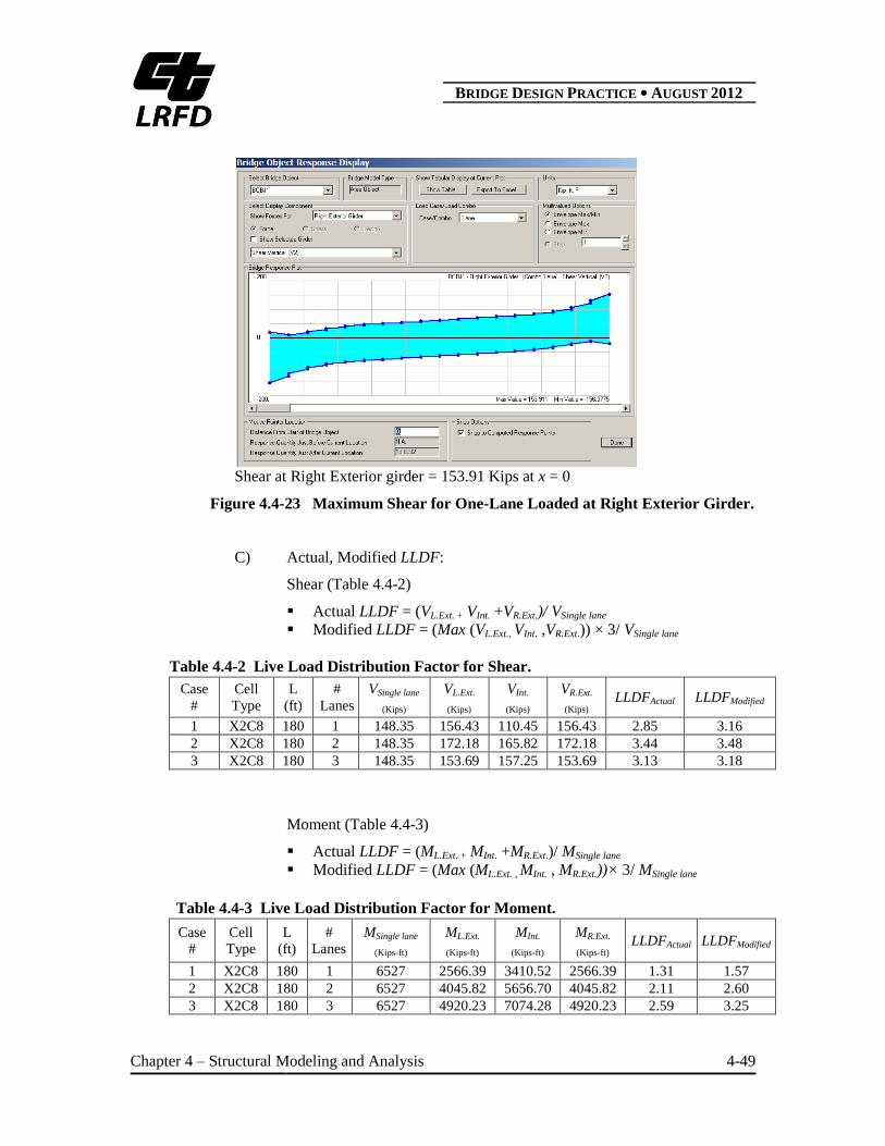
Shear at Right Exterior girder = 153.91 Kips at x = 0

Figure 4.4-23 Maximum Shear for One-Lane Loaded at Right Exterior Girder.

C) Actual, Modified LLDF:

Shear (Table 4.4-2)

Actual LLDF = (VL.Ext. + VInt. +VR.Ext.)/ VSingle lane

Modified LLDF = (Max (VL.Ext., VInt. ,VR.Ext.)) × 3/ VSingle lane

Table 4.4-2 Live Load Distribution Factor for Shear.

Case

#

Cell

Type

L

(ft)

#

Lanes

VSingle lane

(Kips)

VL.Ext.

(Kips)

VInt.

(Kips)

VR.Ext.

(Kips) LLDFActual LLDFModified

1 X2C8 180 1 148.35 156.43 110.45 156.43 2.85 3.16

2 X2C8 180 2 148.35 172.18 165.82 172.18 3.44 3.48

3 X2C8 180 3 148.35 153.69 157.25 153.69 3.13 3.18

Moment (Table 4.4-3)

Actual LLDF = (ML.Ext. + MInt. +MR.Ext.)/ MSingle lane

Modified LLDF = (Max (ML.Ext. , MInt. , MR.Ext.))× 3/ MSingle lane

Table 4.4-3 Live Load Distribution Factor for Moment.

Case

#

Cell

Type

L

(ft)

#

Lanes

MSingle lane

(Kips-ft)

ML.Ext.

(Kips-ft)

MInt.

(Kips-ft)

MR.Ext.

(Kips-ft) LLDFActual LLDFModified

1 X2C8 180 1 6527 2566.39 3410.52 2566.39 1.31 1.57

2 X2C8 180 2 6527 4045.82 5656.70 4045.82 2.11 2.60

3 X2C8 180 3 6527 4920.23 7074.28 4920.23 2.59 3.25



Although the SAP2000/CSI analysis provides a more exact distribution of force

effects in the girders, it doesn’t calculate the amounts of prestressing, longitudinal, or

shear reinforcement required on the contract plans. Different two-dimensional tools

such as CTBridge are used for design. The girders are considered individually, or,

lumped together into a single-spine model.

Caltrans prefers the latter in the case of post-tensioned box girders because post-

tensioning in one girder has an effect on the adjacent girder.

If the individual demands were simply lumped together and used in two-

dimensional software for design and the girders design equally, at least one girder

would be under-designed. Hence, the value from the girder with the highest demand

is used for all girders–as shown above, so it is recommended to consider LDF

Modified, as the Live Load Lanes input for CTBridge.



NOTATION

A = area of section (ft2)

d = structure depth (in.)

E = Young’s modulus (ksi)

g = gravitational acceleration (32.2 ft/sec)

gM = girder LL distribution factor for moment

gS = girder LL distribution factor for shear

H = height of element (ft)

I = moment of inertia (ft4)

Kg = longitudinal stiffness parameter (in.4)

L = span length (ft)

MLL = moment due to live load (k-ft)

MT = transverse moment on column (k-ft)

ML = longitudinal moment on column (k-ft)

MDC = moment due to dead load (k-ft)

MDW = moment due to dead load wearing surface (k-ft)

MHL-93 = moment due to design vehicle (k-ft)

MPERMIT = moment due to permit vehicle (k-ft)

MPS = moment due to Secondary prestress forces (k-ft)

n = modular ratio

Nb = number of beams

Nc = number of cells in the box girder section

S = center-to-center girder spacing (ft)

ts = top slab thickness (in.)

tdeck = deck thickness (in.)

tsoffit = soffit thickness (in.)

tgirder = girder stem thickness (in.)

w = uniform load (k/ft)

X = moment arm for overhang load (ft)

= coefficient of thermal expansion

= skew angle (degrees)



REFERENCES

1. AASHTO, (2007). LRFD Bridge Design Specifications, American Association of State

Highway and Transportation Officials, 4th Edition, Washington, D.C.

2. ADINA, (2010). ADINA System, ADINA R & D, Inc., Watertown, MA.

3. Caltrans, (2008). California Amendments to AASHTO LRFD Bridge Design

Specifications, California Department of Transportation, Sacramento, CA.

4. Caltrans, (1998-2007). CTBRIDGE, Caltrans Bridge Analysis and Design v. 1.3.1,

California Department of Transportation, Sacramento, CA.

5. Caltrans, (2007). Memo to Designers 20-4 - Earthquake Retrofit for Bridges, California

Department of Transportation, Sacramento, CA.

6. CSI, (2007). SAP2000 (Structural Analysis Program) v. 10.1.1, Computers and

Structures, Inc., Berkeley, CA.

7. Barker, R. M. and Puckett, J. A., (2007). Design of Highway Bridges, 2nd Edition, John

Wiley & Sons, Inc., New York, NY.

8. Caltrans, (2010). Seismic Design Criteria, Version 1.6, California Department of

Transportation, Sacramento, CA.

9. Priestley, Seible and Calvi (1996). Seismic Design and Retrofit of Bridges, John Wiley &

Sons, Inc., New York, NY.

10. Chen, W.F. and Duan, L., (1999). “Bridge Engineering Handbook”, CRC Press. Boca

Raton, FL.

Documents

Chapter 4 structure design and analysis