90

CHAPTER 5

MULTI OBJECTIVE OPTIMIZATION IN PSO

5.1 PARTICLE SWARM OPTIMIZATION (PSO) TECHNIQUES

5.1.1 Introduction

Particle swarm optimization (PSO) is a population based stochastic

optimization technique developed by Dr. Eberhart and Dr. Kennedy (1995),

inspired by social behavior of bird flocking or fish schooling. It has been

applied successfully to wide variety of search and optimization problems. It

can be applied to any problem that can be expressed in terms of an objective

function. Similar to GAs, PSO is a population-based optimization tool. The

system is initialized with a population of random solutions and searches for

optima by updating generations. However, unlike GA, PSO has no evolution

operators such as crossover and mutation. In PSO, the solutions, called

particles, are “flown” through the problem space by following the current

optimum particles.

5.1.2 Particle swarm optimization technique

The particle swarm concept originated as a simulation of a

simplified social system. The original intent was to graphically simulate the

choreography of a flock of birds or school of fish. However, the particle

swarm model can be used as an optimizer.

PSO simulates the behavior of bird flocking. Suppose a flock of

birds are randomly searching for food in an area, only one place of food exists

in the area being searched. All the birds do not know where the food is, but

they know how far the food is in each interaction. So what is the best strategy

91

to find the food? The most objective one is to follow the bird nearest to the

food.

PSO learns from this scenario and uses it to solve optimization

problems. In PSO, each single solution is a “bird” in the search space (we call

it a “particle”). All the particles have fitness values that are evaluated by the

fitness function to be optimized and have velocities that direct the “flying” of

the particles. The particles fly through the problem space by following the

current optimum particular.

PSO is initialized with a group of random particles (solutions) and

then searches for optima by updating generations. In every integration, each

particle is updated by following two “best” values. The first one is the best

solution (fitness) it has achieved so far. The fitness value is also stored, this

value is called pbest. Another “best” value tracked by the particle swarm

optimizer is the best value and is called gbest. When a particle takes part of

the population as its topological neighbors, the best value is a local best and is

called lbest is suggested Suganthan (1999).

5.1.3 Adaptation of PSO

In PSO the initial population is randomly generated and combined.

Objective function value is computed for each particle. Then velocity of

each particle is calculated according to the following equation is presented by

Kennedy and Mendes (2003).

l * rand(x) * (pbest [i]- present[i] ) + C2 * rand (x)

* (gbest [i]- present[i] )

92

where,

v [i] : The velocity for the i th particle , represents the distance to be

traveled by this particle from the current position.

inertia weights ranges from 0.8 to 0.9 .

rand (x) is a random number between (0,1)

C1 and C2 are learning factors. C1 = C2 = 2.

Present [i]: The location of the ith particle i.e., particle position.

Pbest [i]: The best previous position of the ith particle is recorded and

represented as pbest[i]

Gbest [i]: The index of the best particle among all the particles in the

population is represented by gbest [i].

The new particle for the next iteration is generated by adding the

velocity with the present particle. This is given in the following equation.

New [i] = present [i ] + v[i]

The combined objective function (COF) value is computed for the

current particle and it is compared with present COF. If the COF value of

current particle is better than the COF of the previous one, the current article

is set as new Pbest. The procedure is carried out for the required number of

iterations to obtain the optimum value.

93

Evaluate initial particles to get

Update velocities for all the particles

Update particle position

Evaluate the updated particle to get

Print the Gbest particle

Stop criteria

End

Generate initial population

No

Yes

5.1.4 Block Diagram for Particle Swarm Optimization

Figure 5.1 Algorithm for Particle Swarm Optimization

5.1.5 Parameter Selection

Parameters selection

Number of particles

The typical range is 20-40. Actually for most of the problems, 10

particles are large enough to get good results. For some difficult or special

problems, one can use 100 or 200 particles as well.

94

Dimension of particles

It is determined by the problem to be optimized.

Range of particles

It is also determined by the problem to be optimized, one can

specify different ranges for different dimension of particles.

Vmax

It determines the maximum change one particle can take during one

iteration. Usually we set the range of the particle as the Vmax for example;

the particle

(x1, x2, x3) x1 belongs [-10,10],

then Vmax = 20.

Learning factors

C1, C2 and C3 are usually taken as 2, But in general, C1, C2 equals

to C3 and ranges from [0,4].

The stop condition

The maximum number of iterations the PSO execute and the

minimum error requirement.

5.2 MINIMUM OPERATION TIME USING PSO

In this example,

x i (L) = 50(rpm) for speed x i (U) = 3500(rpm) for speed

x i (L) = 0.01(mm/rev)for feed x i (U) = 0.4(mm/rev) for feed

x i (L) =0.3(mm) for depth of cut x i (U) = 1.5(mm) for depth of cut

95

Table 5.1 Optimized values of operation time in PSO

Iteration

(no.)

Speed

(rpm)

Feed

(mm/rev)

Depth of cut

(mm)

Op Time

(min)

1 1692.857 0.196 0.852 3.191

2 1473.81 0.245 0.7 3.175

3 1692.857 0.27 0.814 3.138

4 1254.762 0.394 0.548 3.128

5 2788.095 0.233 0.776 3.098

6 1692.857 0.381 0.51 3.098

7 1692.857 0.394 0.3 3.097

8 1747.619 0.369 0.814 3.095

9 3445.238 0.233 0.51 3.079

Table 5.1 shows the best result among all the iteration using

particle swarm optimization algorithm for minimum operation time. Table

indicates the optimum cutting parameters for each iteration and given the

optimum value for minimum operation time.

Table 5.2 Best optimum value for operation time in PSO

Speed

(m/min)

Feed

(mm/rev)

Depth of cut

(mm)

Op Time

(min)

3445.238 0.233 0.51 3.079

The resulted optimize cutting parameters from Table 5.1is

presented in the Table 5.2. It shows the optimum operation time of 3.079 min.

96

Output

Figure 5.2 Pareto front - operation time Vs iteration

The Pareto front graph of operation time and iteration is shown in

the Figure 5.2. Among 100 iterations the best solutions are obtained in 9

populations. The curve decreases gradually from 3.191 min to 3.12 min and

makes small variations thereafter and gives the optimum value at 3.079 min.

Figure 5.3 Operation time Vs Feed Vs Depth of cut

97

Figure 5.3 shows the three dimensional view of optimum operation

time, feed and depth of cut and shows the minimum operation time of 3.079

min and feed 0.233mm/rev and optimum depth of cut 0.51mm.

Figure 5.4 Speed Vs Feed Vs Depth of cut - Operation Time.

The three dimensional view of optimum cutting parameters of

speed, feed and depth of cut are indicated in Figure 5.4. It shows the optimum

value of speed 3445.238 rpm, feed 0.233 mm/rev and depth of cut 0.51 mm

for minimum operation time.

5.3 MINIMUM TOOL WEAR USING PSO

In this example,

x i (L) = 50 for speed x i(U) = 3500 for speed

x i (L) = 0.01for feed x i (U) = 0.4 for feed

x i (L) =0.3 for depth of cut x i(U) = 1.5 for depth of cut

98

Table 5.3 Optimized values of tool wear in PSO

Iteration (no.)

Speed(rpm)

Feed(mm/rev)

Depth of cut (mm)

Tool wear (µ)

1 3335.714 0.332 1.271 0.692

2 3335.714 0.295 0.967 0.691

3 3335.714 0.27 1.31 0.674

4 3007.143 0.295 1.5 0.63

5 3335.714 0.233 0.967 0.602

6 3335.714 0.233 0.967 0.547

7 1911.905 0.394 1.271 0.536

8 3335.714 0.134 1.005 0.536

9 3335.714 0.134 1.176 0.453

Table 5.3 indicates the best result among the iterations and gives

the best combination among the speed, feed and depth of cut for the minimum

tool wear.

Table 5.4 Optimal cutting parameters for minimum tool wear

Speed

(rpm)

Feed

(mm/rev)

Depth of cut

(mm)

Tool wear

(µ)

3335.714 0.134 1.176 0.453

Table 5.4 indicates minimum tool wear among all the values with

the optimized feed, speed and depth of cut and shows the optimum tool wear

is 0.453.

99

Output

Figure 5.5 Pareto front curve - tool wear Vs population

Figure 5.5 shows the Pareto front curve for tool wear and

population. Tool wear decreases gradually with the optimized speed of

3335.714 rpm, feed 0.134 mm/rev and with the depth of cut 1.176 mm and

finally minimized to 0.453 µ.

Figure 5.6 Speed Vs Feed Vs Depth of cut - Tool wear

100

Figure 5.6 indicates the three dimensional view of optimum cutting

parameters of speed, feed and depth of cut and indicates the optimum values

of speed 3335.714 rpm, feed 0.134 mm/rev and depth of cut 1.176 mm for

minimum tool wear. The graph also indicates the several situations and

facilitating the right parameters for any condition.

5.4 MINIMUM UNIT COST USING PSO

In this example,

x i (L) = 50 for speed x i (U) = 3500 for speed

x i (L) = 0.01for feed x i (U) = 0.4 for feed

x i (L) =0.3 for depth of cut x i (U) = 1.5 for depth of cut

Table 5.5 Output result of minimum production cost

Iteration

(no.)

Speed

(rpm)

Feed

(mm/rev)

Depth of cut

(mm)

Unit Cost

(Rs)

1 3445.238 0.233 0.51 2.507

2 1747.619 0.369 0.814 2.196

3 1692.857 0.394 0.3 1.953

4 2788.095 0.233 0.776 1.754

5 1692.857 0.381 0.51 1.706

6 1254.762 0.394 0.548 1.706

7 1692.857 0.27 0.814 1.678

8 1473.81 0.245 0.7 1.606

9 1692.857 0.196 0.852 1.597

101

UC (Rs)

Table 5.5 shows the best result among all the 100 iteration and

gives the best combination among the speed, feed and depth of cut for the

minimum production cost.

Table 5.6 Optimized result of production cost

Speed

(rpm)

Feed

(mm/rev)

Depth of cut

(mm)

Unit Cost

(Rs)

1692.857 0.196 0.852 1.597

Table 5.6 indicates minimum production cost among all the values

with the optimized feed, speed and depth of cut and shows the optimum

production cost is Rs.1.597.

Output

Figure 5.7 Pareto front curves for unit cost and population

102

Figure 5.7shows the Pareto front curve of unit cost and population.

Figure shows the 9 population and the cost decreases gradually up to 4

populations at the unit cost of Rs. 2.5 and again decreases with minor

variation and finally optimized at the cost Rs.1.597.

Figure 5.8 Speed Vs Feed Vs Depth of cut - Production cost.

Figure 5.8 indicates the three dimensional view of optimum cutting

parameters of speed, feed and depth of cut and indicates the optimum value of

speed 1692.857 rpm, feed 0.196 mm/rev and depth of cut 0.852 mm for

minimum production cost.

5.5 MINIMUM PRODUCTION COST & OPERATION TIME

USING PSO

In this example,

x i (L) = 50 for speed x i(U) = 3500 for speed

x i (L) = 0.01for feed x i (U) = 0.4 for feed

x i (L) =0.3 for depth of cut x i(U) = 1.5 for depth of cut

103

Table 5.7 Optimized values of production cost & operation Time in

PSO

Iteration

(no.)Speed(rpm)

Feed(mm/rev)

Depth of cut (mm)

Op Time(min)

Unit Cost (Rs)

Rank

1 3445.238 0.233 0.51 3.079 2.507 1

2 1747.619 0.369 0.814 3.095 2.196 1

3 1692.857 0.394 0.3 3.097 1.953 1

4 2788.095 0.233 0.776 3.098 1.754 1

5 1692.857 0.381 0.51 3.098 1.706 1

6 1254.762 0.394 0.548 3.128 1.706 1

7 1692.857 0.27 0.814 3.138 1.678 1

8 1473.81 0.245 0.7 3.175 1.606 1

9 1692.857 0.196 0.852 3.191 1.597 1

Table 5.7 indicates the output result between minimum operation

time and minimum production cost. Table shows the best result among all the

100 iteration and gives the best combination among the speed, feed and depth

of cut for 9 populations. All the optimized combinations are tabulated.

Table 5.8 Best optimum value for operation time & production cost

Speed

(rpm)

Feed

(mm/rev)

Depth of cut

(mm)

Op Time

(min)

Unit Cost

(Rs)

Rank

3445.238 0.233 0.51 3.079 2.507 1

Table 5.8 shows the optimized value between the operation time

and production cost with the optimal cutting parameters and shows the

minimum operation time 3.079 min and minimum production cost Rs. 2.507.

104

UC (Rs)

Output

Figure 5.9 Pareto front curve - Operation time Vs Production cost

Figure 5.9 indicates the Pareto front curve for operation time and

production cost. Graph shows the minimum operation time for 3.079min and

the production cost is Rs. 2.507. The curve also indicates the several different

situations, facilitating the choice of right parameters for any condition.

Figure 5.10 Speed, Feed and Depth of cut for operation time and

production cost

105

Figure 5.10 indicates the three dimensional view of optimum

cutting parameters of speed, feed and depth of cut and indicates the optimum

value of speed 3445.238 rpm, feed 0.233 mm/rev and depth of cut 0.51mm

for operation time and production cost.

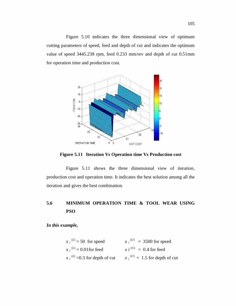
Figure 5.11 Iteration Vs Operation time Vs Production cost

Figure 5.11 shows the three dimensional view of iteration,

production cost and operation time. It indicates the best solution among all the

iteration and gives the best combination.

5.6 MINIMUM OPERATION TIME & TOOL WEAR USING

PSO

In this example,

x i (L) = 50 for speed x i(U) = 3500 for speed

x i (L) = 0.01for feed x i (U) = 0.4 for feed

x i (L) =0.3 for depth of cut x i(U) = 1.5 for depth of cut

106

Table 5.9 Optimized values for production time & tool wear in PSO

Iteration

(no.)

Speed

(rpm)

Feed

(mm/rev)

Depth of cut

(mm)

Op Time

(min)

Tool wear

(µ) Rank

1 3335.714 0.332 1.271 3.057 0.692 1

2 3335.714 0.295 0.967 3.064 0.691 1

3 3335.714 0.27 1.31 3.07 0.674 1

4 3007.143 0.295 1.5 3.071 0.63 1

5 3335.714 0.233 0.967 3.081 0.602 1

6 3335.714 0.233 0.967 3.081 0.547 1

7 1911.905 0.394 1.271 3.084 0.536 1

8 3335.714 0.134 1.005 3.142 0.536 1

9 3335.714 0.134 1.176 3.142 0.453 1

Table 5.9 indicates the output result of minimum operation time

and minimum tool wear. Table show the best result among all the iteration

and show the best population. It gives the best combination among the cutting

parameters.

Table 5.10 Best Optimum value - Operation time & Tool wear

Speed(rpm)

Feed(mm/rev)

Depth of cut (mm)

Op Time (min)

Tool wear (µ) Rank

3335.714 0.332 1.271 3.057 0.692 1

107

Table 5.10 shows the optimized value between the operation time

and tool wear with the best combination of speed, feed and depth of cut.

Output

Figure 5.12 Operation time Vs Tool wear - Pareto front curve

Figure 5.12 shows the Pareto front curve for operation time and

tool wear. Figure shows clearly that the tool wear is decreased gradually in

the initial iteration and then constant in further iteration. Graph shows the

optimized operation time 3.057 min and tool wear 0.692 µ. The curve also

indicates and facilitates the choice of right parameter for any condition.

108

Figure 5.13 Speed, Feed and Depth of cut for operation time and

tool wear

Figure 5.13 indicates the three dimensional view of optimum

cutting parameters of speed, feed and depth of cut and indicates the optimum

value of speed 3335.714 rpm, feed 0.332 mm/rev and depth of cut 1.271mm

for operation time and tool wear.

Figure 5.14 Speed Vs Depth of cut Vs Tool wear

109

Figure 5.14 indicates the three dimensional view of optimum

cutting parameters of speed and depth of cut for tool wear.

Figure 5.15 Depth of cut for operation time and tool wear

Figure 5.15 indicates the optimum depth of cut for operation time

and tool wear and clearly shows that when the depth of cut increases the tool

wear also increases.

Figure 5.16 Optimum feed for operation time and tool wear

110

Figure 5.16 shows the optimum feed for operation time and tool

wear and clearly shows that when the feed increases the tool wear also

increases.

Figure 5.17 Speed for operation time and tool wear

Figure 5.17 shows the optimum cutting speed for operation time

and tool wear. The optimum cutting speed can be identified through the graph

and any selected speed can be analyzed using this graph.

5.7 MINIMUM COST & TOOL WEAR USING PSO

In this example,

x i (L) = 50 for speed x i(U) = 3500 for speed

x i (L) = 0.01for feed x i (U) = 0.4 for feed

x i (L) =0.3 for depth of cut x i(U) = 1.5 for depth of cut

111

Table 5.11 Optimized values of production cost & tool wear in PSO

Iteration

(no.)Speed (rpm)

Feed (mm/rev)

Depth of cut (mm)

Unit cost (Rs)

Tool wear (µ)

Rank

1 3445.238 0.233 0.51 2.507 0.692 1

2 1747.619 0.369 0.814 2.196 0.691 1

3 1692.857 0.394 0.3 1.953 0.674 1

4 2788.095 0.233 0.776 1.754 0.63 1

5 1692.857 0.381 0.51 1.706 0.602 1

6 1254.762 0.394 0.548 1.706 0.547 1

7 1692.857 0.27 0.814 1.678 0.536 1

8 1473.81 0.245 0.7 1.606 0.536 1

9 1692.857 0.196 0.852 1.597 0.453 1

Table 5.11 shows the output result of production cost and tool wear

for different combination of cutting parameters. It shows the best solution

among all the iterations and gives the best combination among the speed, feed

and depth of cut for 9 populations.

Table 5.12 Best Optimum value for production cost & tool wear

Speed (rpm)

Feed (mm/rev)

Depth of cut (mm)

Unit cost (Rs)

Tool wear (µ)

Rank

1692.857 0.196 0.852 1.597 0.453 1

The optimized cutting parameter resulted from the Table 5.11 is

shown in Table 5.12. It represents the optimized value for production cost and

tool wear.

112

Output

Figure 5.18 Pareto front curves - Tool wear Vs Production cost

Figure 5.18 indicates the Pareto front curve for unit cost and tool wear. It is evident that the tool wear is decreasing gradually and reach the optimum wear. The graph shows the optimum value of cost Rs.1.754 and optimum tool wear 0.63µ. It also indicates the several different combinations.

Figure 5.19 Speed, feed and depth of cut for production cost and tool

wear

UC (Rs)

113

Figure 5.19 indicates the three dimensional view of optimum

cutting parameters of speed, feed and depth of cut and indicates the optimum

value of speed 2788.095 rpm, feed 0.233 mm/rev and depth of cut 0.776 mm

for production cost and tool wear.

Figure 5.20 Optimum speed Vs production cost Vs tool wear

Figure 5.20 indicates the three dimensional view of speed, unit cost

and tool wear. It shows the optimum speed for tool wear and cost.

5.8 OPTIMUM PRODUCTION COST, OPERATION TIME AND

TOOL WEAR USING PSO

In this example,

x i (L) = 50 for speed x i (U) = 3500 for speed

x i (L) = 0.01for feed x i (U) = 0.4 for feed

x i (L) =0.3 for depth of cut x i (U) = 1.5 for depth of cut

114

Table 5.13 Optimized values of Production cost, Operation time & Tool

wear

Iteration(no.) Speed

(rpm) Feed

(mm/rev)

Depth of cut(mm)

Op Time (min)

Unit Cost(Rs)

Tool wear (µ)

Rank

1 3445.238 0.233 0.51 3.079 2.507 0.692 1

2 1747.619 0.369 0.814 3.095 2.196 0.691 1

3 1692.857 0.394 0.3 3.097 1.953 0.674 1

4 2788.095 0.233 0.776 3.098 1.754 0.63 1

5 1692.857 0.381 0.51 3.098 1.706 0.602 1

6 1254.762 0.394 0.548 3.128 1.706 0.547 1

7 1692.857 0.27 0.814 3.138 1.678 0.536 1

8 1473.81 0.245 0.7 3.175 1.606 0.536 1

9 1692.857 0.196 0.852 3.191 1.597 0.453 1

Table 5.13 shows the output result between the operation time,

production cost and tool wear. PSO implementation produces best result among

all the iterations and gives the best population. The table also indicates the

different combination of machining parameters and gives the optimum solution.

Table 5.14 Best Optimum value for operation time, tool wear and

production cost

Speed (rpm)

Feed(mm/rev)

Depth of cut (mm)

Op Time (min)

Unit Cost (Rs)

Tool wear (µ)

Rank

2788.095 0.233 0.776 3.098 1.754 0.63 1

The optimized cutting parameter resulted from the Table 5.13 is shown in

Table 5.14. It shows the minimum operation time 3.098 min and tool wear

0.63µ with the production cost Rs.1.754.

115

Output

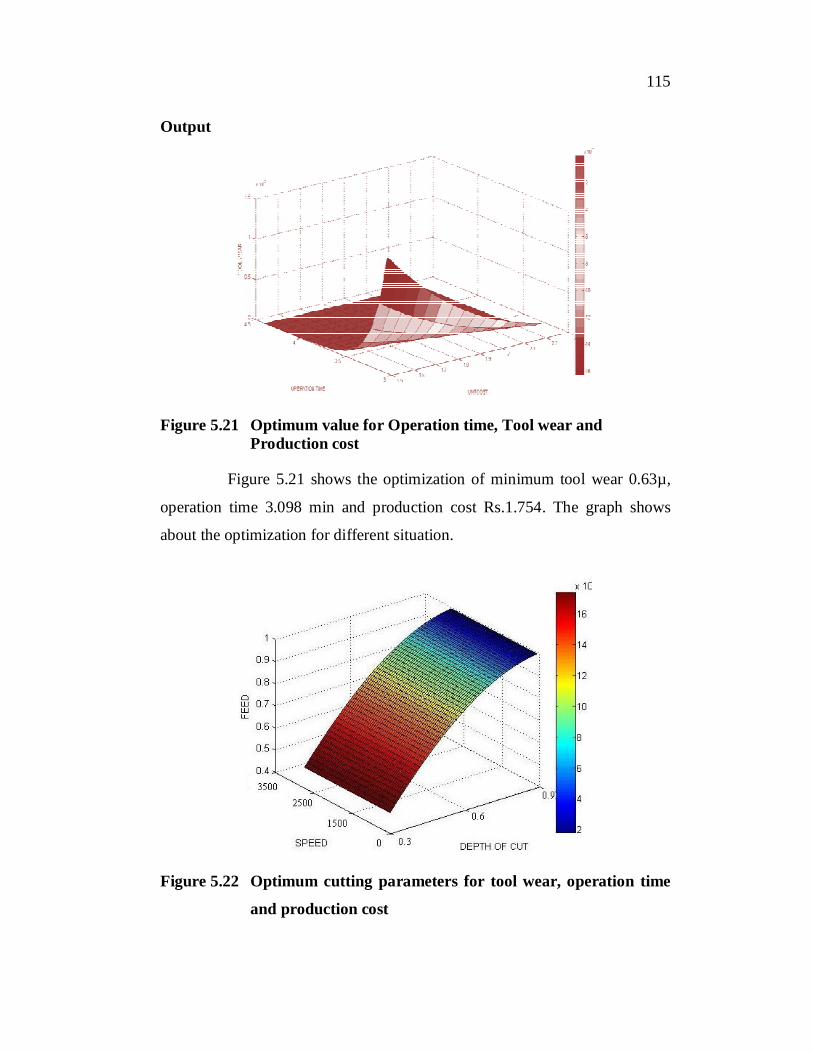
Figure 5.21 Optimum value for Operation time, Tool wear andProduction cost

Figure 5.21 shows the optimization of minimum tool wear 0.63µ,

operation time 3.098 min and production cost Rs.1.754. The graph shows

about the optimization for different situation.

Figure 5.22 Optimum cutting parameters for tool wear, operation time

and production cost

116

Figure 5.22 shows the optimum cutting parameters for optimum

tool wear, operation time and cost. The curve facilitates the choice of right

parameter for any condition.

5.9 RESULTS AND DISCUSSION

Particle swarm optimization is an optimization technique which

will produce the best optimized results for any discrete problems. Particle

swarm optimization deals with selecting the best results by pbest and gbest

method. The partial best populations are predicted in this pbest module.

Global best solutions are carried by gbest module. The PSO techniques

carried out by 100 iteration and 9 best populations are predicted for this

problem to get the good results.

Table 5.1 indicates the best result among all the iteration. The

minimum operation time among all the iterations with the optimized feed,

speed and depth of cut and the operation time of 3.079 min are shown in

Table 5.2. The Pareto front graph of operation time and iteration is plotted in

Figure 5.2. Three dimensional view of optimum operation time, feed and

depth of cut are shown in Figure 5.3. Three dimensional views of optimum

cutting parameters of speed, feed and depth of cut for minimum operation

time is shown in Figure 5.4.

Table 5.3 indicates the best result among the iterations and gives

the best combination among the speed, feed and depth of cut for the minimum

tool wear. Table 5.4 shows the minimum tool wear of 0.453 µ among all the

values with the optimized feed, speed and depth of cut. Figure 5.5 shows the

Pareto front curve for tool wear and population. The optimum cutting

parameters of speed, feed and depth of cut for minimum tool wear are given

in Figure 5.6.

117

Table 5.5 shows the best result among all the 100 iteration and

gives the best combination among the speed, feed and depth of cut for the

minimum production cost. Table 5.6 indicates minimum production cost

among all the values with the optimized feed, speed and depth of cut and

shows the optimum production cost is Rs. 1.597. The Pareto front curve of

unit cost and population is shown in Figure 5.7. The graphical representation

of optimum cutting parameters of speed, feed and depth of cut is depicted in

Figure 5.8.

Table 5.7 indicates the output result between optimum operation

time and optimum production cost. Optimized value between the operation

time and production cost are shown in Table 5.8. Pareto front curve for

operation time and production cost is shown in Figure 5.9, the curve

facilitating the right parameter for any condition. Figure 5.10 shows the

graphical representation of optimum cutting parameters of speed, feed and

depth of cut for operation time and production cost. Figure 5.11 shows the

three dimensional view graph of Iteration Vs Objective functions such as

Operation time and Production cost.

Table 5.9 indicates the output result of minimum operation time

and minimum tool wear. The optimized value between the operation time and

tool wear is given in Table 5.10. Pareto front curve for operation time and tool

wear is shown in Figure 5.12. The optimum cutting parameters of speed, feed

and depth of cut for tool wear and operation time are shown in Figure 5.13.

The optimum speed and depth of cut for tool wear is shown in the Figure

5.14. Optimum depth of cut for operation time and tool wear is depicted in

Figure 5.15. The optimum feed for operation time and tool wear is shown in

Figure 5.16 and Figure 5.17 shows the optimum cutting speed for operation

time and tool wear.

118

Table 5.11 shows the output result of production cost and tool wear

for different combination of cutting parameters. Table 5.12 shows the

optimized value for production cost and tool wear with the optimal cutting

parameters and indicates the optimized production cost and tool wear. The

Pareto front curve for unit cost and tool wear is shown in Figure 5.18 and

Figure 5.19 indicates the speed, feed and depth of cut for production cost and

tool wear. Optimum cutting speed for tool wear and production cost are given

in Figure 5.20.

Table 5.13 indicates the output result between the operation time,

production cost and tool wear. Table 5.14 shows the optimized cutting

parameters for operation time, production cost and tool wear. Table shows the

minimum operation time 3.098 min and tool wear 0.63µ with the production

cost Rs.1.754. Figure 5.21 indicates the graphical representation of multi

objective optimization with minimum tool wear, operation time and

production cost. The graph shows the clear information about the

optimization for different situation. Figure 5.22 shows the optimum cutting

parameters for optimum tool wear, operation time and cost.